MULTIVIEW DEPTH CODING BASED ON

COMBINED COLOR/DEPTH SEGMENTATION

J. Ruiz-Hidalgoa, J.R. Morrosa, P. Aflaki B.b, F. Caldereroc, F. Marquesa

aDepartment of Signal Theory and CommunicationsUniversitat Politecnica de Catalunya

Jordi Girona 1-3, 08034, Barcelona, SpainFax: +34 9 3401 6447, Phone: +34 9 3401 6440

Email: {j.ruiz, ramon.morros, ferran.marques}@upc.edubTampere University of Technology, Tampere, Finland

Email: payman.aflaki@tut.ficUniversitat Pompeu Fabra, Tanger 122, 08018, Barcelona, Spain

Email: felipe.calderero@upf.edu

Abstract

In this paper a new coding method for multiview depth video is presented.

Considering the smooth structure and sharp edges of depth maps, a seg-

mentation based approach is proposed. This allows further preserving the

depth contours thus introducing fewer artifacts in the depth perception of the

video. To reduce the cost associated with partition coding, an estimation of

the depth partition is built using the decoded color view segmentation. This

estimation is refined by sending some complementary information about the

relevant differences between color and depth partitions. For coding the depth

content of each region, a decomposition into orthogonal basis is used in this

paper although similar decompositions may be also employed. Experimen-

tal results show that the proposed segmentation based depth coding method

outperforms H.264/AVC and H.264/MVC by more than 2dB at similar bi-

trates.

Keywords: Depth map, virtual view, multiview video coding, 3DTV

Preprint submitted to Elsevier April 20, 2011

1. Introduction

It is believed that 3D is the next major revolution in the history of TV.

Both at professional and consumer electronics exhibitions, companies are ea-

ger to show their new 3D applications. In these applications, the 3D effect is

obtained by recording the scene from multiple viewpoints, which is referred

as Multi-View Video (MVV) [1]. MVV information is often completed with

sample depth information (depth maps) for each view, thus conforming the

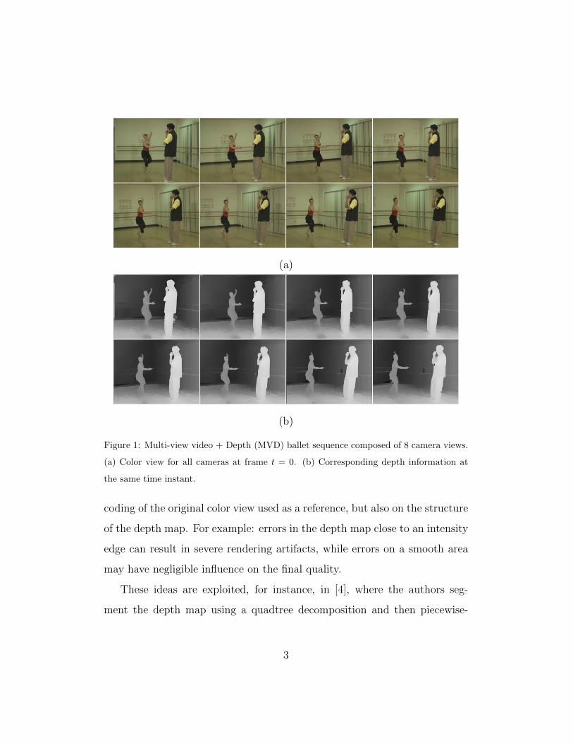
Multi-view Video + Depth (MVD) format (Fig. 1). The introduction of this

MVD format allows the incorporation of new functionalities such as Free

View Point Video [2] in current 3DTV applications. MVD representations

result in a vast amount of data to be stored or transmitted. In most situ-

ations, there is a need to compress these data efficiently without sacrificing

visual quality significantly. Previous works presented various solutions for

MVV coding (MVC) [3], mostly based on H.264 with combined temporal

and inter-view prediction. Also, approaches for depth map coding in MVD

have been proposed [4, 5, 6].

In 3D applications, depth maps are used for rendering new images (virtual

color views) but not to be directly viewed by the end user. Thus, the goal

when coding depth maps is to maximize the perceived visual quality of the

rendered virtual color views instead of the visual quality of the depth maps

themselves [4]. Traditional image compression methods have been designed

to provide maximum perceived visual quality, so using these methods to

compress depth maps may result in suboptimal performance. The rendering

error depends on the quality of the depth map coding and the quality of the

2

(a)

(b)

Figure 1: Multi-view video + Depth (MVD) ballet sequence composed of 8 camera views.

(a) Color view for all cameras at frame t = 0. (b) Corresponding depth information at

the same time instant.

coding of the original color view used as a reference, but also on the structure

of the depth map. For example: errors in the depth map close to an intensity

edge can result in severe rendering artifacts, while errors on a smooth area

may have negligible influence on the final quality.

These ideas are exploited, for instance, in [4], where the authors seg-

ment the depth map using a quadtree decomposition and then piecewise-

3

linear functions are used to represent the depth information in each resulting

block. Even though their experimental results show coding gains compara-

ble to AVC with no temporal prediction (using only I frames) and MVC,

costly partition information for the quadtree must be sent which results in

a reduction of the performance. Another approach exploiting the previous

ideas is presented in [7]. It relies on a shape-adaptive discrete wavelet trans-

form (SA-DWT). The contours of the depth maps are extracted using a

Canny edge detector and encoded using a differential Freeman chain-code.

SA-DWT greatly reduces the data entropy of the resulting coefficients and

the experimental results show significant coding gains with respect to tra-

ditional techniques based on DWT. However, a formal comparisons against

the AVC standard is not provided. In [5], the authors proposed a combined

representation, called layered depth image (LDI), for color views and depth

in MVD sequences. As the LDI representation aims to reduce the redundant

information between camera views, it is very useful for coding purposes.

However, the number of layers for each element in the representation must

be encoded lossless or near-lossless which limits its coding efficiency. Also,

the LDI representation is more suited to scenarios with cameras close to each

other.

Our proposal is inspired on segmentation-based coding systems (SBCS) [8].

These systems partition images (in this case, depth maps) into a set of ar-

bitrarily shaped homogeneous regions. The separate coding of each region

allows reducing the coding artifacts due to sharp edges and, hence, it is very

appropriate to encode depth maps. As the need to send the partition infor-

mation (shape of the regions) to the decoder is one of the major efficiency

4

drawbacks of SBCS, we present a novel solution that greatly reduces the cost

associated to depth partition coding using the fact that the depth partition

can be estimated using the decoded image color partition. Experimental re-

sults in Section 3 will show that the proposed method outperforms AVC and

MVC when encoding MVD sequences.

This paper is organized as follows. Section 2 describes the approach

proposed to encode depth maps in multiview sequences using a segmentation

based technique. Section 3 presents the experimental results comparing our

method with AVC and MVC. Finally, Section 4 provides some conclusions

and future extensions of this work.

2. Segmentation based depth encoding approach

Our proposal is based on segmenting the depth map into homogeneous

regions of arbitrary shape and then coding the contents of these regions using

texture coding techniques [8]. For simplicity, in the sequel we will use the

word texture to refer to the depth information inside the regions. As can

be seen in Fig. 1, depth maps can be considered approximately piecewise

planar, with highly homogeneous regions separated by strong contours. The

resulting regions can be efficiently encoded using low order methods, like

piecewise linear functions in the case of [4] or a decomposition into orthogonal

bases in our approach.

Having uniform regions will allow coding the depth values (texture) in-

side the region with only a few coefficients. However, as the receiver does

not know the shape of the resulting regions, the partition must be encoded

and transmitted. To avoid the high cost associated to coding the resulting

5

partitions (region shape), instead of directly segmenting the depth map (as in

other approaches, like [4]), the novel idea we are proposing is to approximate

the depth partition from the decoded color partition, and to send only the

information about the relevant difference between both partitions. As it will

be shown, this will result in a very efficient coding of the depth partition.

In this process we make two assumptions: a) the color views have been

previously coded and sent to the receiver (decoded color views), and b) we can

always construct a color partition (generated using only color information)

such that it contains the important depth transitions. This is, a homogeneous

region in the color partition will also result in a homogeneous region in the

depth partition. This ensures that depth regions can be encoded efficiently.

Assumption b) is not straightforward and needs further reasoning: In

most cases, strong transitions in the depth maps coincide with color tran-

sitions in the color views because objects at different depths usually have

different color or illumination conditions. Figs. 2.a and 2.b show a compari-

son between partitions computed on the color and depth images, both with

the same number of regions. The strong depth transitions, separating both

persons from the background, are also present in the color partition.

By using very fine color partitions, that is, with a high enough number

of regions, as in Fig. 2.c, it can be ensured that almost all relevant contours

in the depth partition are also present in the color view partition.

There are some cases where b) does not hold. One is when objects in

the foreground have the same color as the background. The other is when

objects with uniform color but slowly changing depth (i.e. walls or floors) are

present in the image.

6

(a) (b)

(c)

Figure 2: Comparison between a color partition and the corresponding depth partition at

the same time instant. (a) Partition obtained using color homogeneity and (b) partition

obtained using depth homogeneity for Ballet using 80 regions in each case. Finally, (c) is

a color-based fine partition with 500 regions.

In the first case, our method will under-segment this zone and the coding

will be less efficient because of a non-homogeneous region and the coded

depth may have errors at the depth transitions, which can result in a quality

7

loss at the rendered image. This effect can be seen, for instance, in Figs. 2.a

and 2.b due to the similar color of the ballerina’s hand and the wood handle

at the bottom wall. The second case can be seen in Figs. 2.a and 2.b where,

on the background (wall and floor) the shape of the color and depth regions

differ. However, this does not result in quality loss because both partitions

have smooth and low contrasted regions that can be efficiently coded.

Using the previous assumptions, a color view partition can be constructed

both at the encoder and at the decoder that will contain all the significant

contours in the depth partition (and probably, many more). We use the

decoded color views also at the encoder side to ensure the same partitions are

used at both sides. To further ensure region homogeneity when this partition

is applied to the depth information, we construct it with a high number of

regions (Fig. 2.c). This partition will be used to estimate the final depth

partition. Looking at Fig. 2.c it is obvious that the color view partition

is over-segmented with respect to the depth partition. This is caused by

regions with similar depth but different color. Over-segmentation may result

in coding inefficiency because of the large number of texture coefficients due

to extra regions. By merging some of the regions of the decoded color view

partition, a very good approximation to the optimal depth map partition

can be constructed. That is, to get a better approximation of the depth map

partition, we influence the color view segmentation process using information

from the original depth map available only at the encoder. In this case, some

side information must be sent to the decoder but its amount is small with

respect to directly coding the depth map partition.

8

2.1. Color-depth based segmentation algorithm

Our segmentation technique is based on a region-merging approach. Start-

ing from an initial partition with a high number of regions (or even starting

at the pixel level), the partition is constructed using an iterative process: at

each iteration, the two more similar regions are merged. By stopping the

merging process at a given level, we can obtain a partition with any desired

number of regions.

The similarity measure is computed for each pair of neighboring regions.

In our approach, region similarity is evaluated by comparing the models (for

instance, region means) of the initial regions with the model of the resulting

region after merging. The comparison criterion is the weighted euclidean

distance between region models (WEDM [10]). For two regions R1 and R2,

with areas A1 and A2 respectively, the WEDM cost, OWEDM is given by:

OWEDM(R1, R2) = A1‖MR1 −MR1∪R2‖2 + A2‖MR2 −MR1∪R2‖2 (1)

where the model MRifor region Ri is the vector formed by the average of all

pixels values I(p) with p ∈ Ri:

MRi=

1

Ai

∑p∈Ri

I(p) (2)

The models can be computed on the YCbCr color space if segmentation

is performed using color information or directly on the depth channel when

depth information is used for depth segmentation In the first case, the cost

will be referred as OCWEDM and in the second case as OD

WEDM .

9

Figure 3: Example of final partition with 80 regions.

To create the final depth partition we use a process consisting of an

estimation using a fine color partition and in a set of region mergings to

better approximate the depth partition. This process can be described in

three steps:

First step: A fine initial color view partition (initial partition) is built in

the same way both at the encoder and the decoder (using the decoded color

view) selecting a number of regions high enough to avoid under-segmentation

(see Fig. 2.c). Section 2.1.1 details the algorithm used to determine the

number of regions. This initial partition can be considered an estimation of

the final depth partition and, since it can be constructed both at the encoder

at the decoder, has no coding cost.

Second step: The final partition (Fig. 3) is obtained at the encoder

side by using the aforementioned algorithm with WEDM cost in the depth

10

(R1, R2)→ R6 (R6, R4)→ R7 (R3, R5)→ R8

R1

R2

R3

R4

R5

R6

R3

R4

R5R7

R3

R5R7

R8

(a) (b) (c) (d)

Figure 4: Example of creating a final partition of 2 regions. (a) Example of an initial

partition computed from decoded color information using 5 regions. (b) First iteration

after merging regions R1 and R2. (c) Second iteration after merging R6 and R4. (d) Final

partition with 2 regions after all mergings have been performed.

information (ODWEDM) starting from the initial partition constructed from

the decoded color view. Using an initial partition constructed using only

depth information would be optimal but the shape of this partition would

need to be sent, at a high coding cost. The number of regions in the final

partition is computed similarly to the initial partition (Section 2.1.1). The

difference is that, for the initial partition, the criterion to select the number

of regions was solely to avoid under-segmentation while in the case of the

final partition, a number of regions suitable for coding purposes must be

obtained.

Fig. 4 shows an example of the process followed by the encoder to compute

a final partition of 2 regions. Starting from the initial partition represented in

Fig. 4.a, the algorithm selects to merge the two regions with lowest OWEDM

costs (eq. 1) computed in the original depth information (ODWEDM). In the

first iteration, the lowest cost correspond to regions R1 and R2 so they are

merged in a new region R6 (Fig. 4.b). The next step recomputes the ODWEDM

costs for the new region R6 and selects again the lowest cost for the next

11

merging. In the example, regions R6 and R4 are merged to R7. The process

is iterated until the final number of regions is found and the final partition

is computed as in Fig. 4.d.

Third step: Even if the final partition is constructed from the initial

partition, the decoder can not directly construct this partition because the

depth information is not available. For that, the encoder re-computes the

final partition but, this time, the decoded color information is used to cal-

culate the OWEDM costs. At each iteration, the algorithm selects the two

regions with lowest OCWEDM cost to be merged but, if the two regions are

not merged in the final partition, the merge is prevented and some side in-

formation is sent to inform the decoder so it is able to reproduce the final

partition without the depth information. The side information is composed

of a list of merging orders (called non-merging orders in this paper that in-

form the decoder if a given merge must be allowed or prevented. After a

prevented merge, the next two more similar regions are examined until a

suitable merging is obtained.

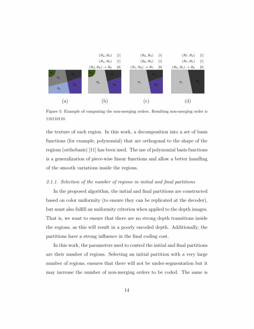
Fig. 5 illustrates this process. Starting from the same initial partition

(Fig. 4.a) as in the second step, regions are merged based on their color

similarity. For instance, in the first iteration, the lowest OCWEDM cost corre-

sponds between regions R2 and R3 (note that this first iteration is different

than in the second step as the decoded color information is used to compute

the cost). As regions R2 and R3 are not merged in the final partition com-

puted in the previous step (Fig. 4.d) the merge is prevented (a 1 is stored in

the non-merging orders list) and the next OCWEDM cost is analyzed. In the

example, the next lower costs correspond to regions R4 and R5. This merging

12

is also prevented. All following costs are analyzed until one corresponding to

two regions that have also been merged in the final partition. In the exam-

ple, regions R2 and R4 are merged into region R6 (Fig. 5.b) and a value of

0 is stored in the non-merging orders list. The process is iterated (Fig. 5.c)

until the final number of regions (the same as the final partition) is achieved

which results in a non-merging order of 110110110. The partition obtained

in Fig. 5.d is identical to the final partition computed previously (Fig. 4.d).

It is a reasonable approximation to a partition obtained using only depth

information (without using the initial partition) while largely reducing the

cost associated to partition coding.

The non-merging orders can be used in the decoder to replicate the en-

coder partition without any depth information. The cost associated to the

non-merging orders is the only information needed for partition coding and

its cost is very low compared to fully encoding the optimal depth partition.

In our example, even though the worst possible scenario has been selected,

only 9 bits are needed to encode the entire final partition. In real images,

the associated cost OCWEDM and OD

WEDM between two regions may be similar

and the length of the non-merging orders would be reduced. Also, the prob-

ability of prevent mergings (denoted as 1 in the non-merging orders) is low

(around 0.2 for our test sequences) thus allowing for a further compression

using arithmetic coding.

The actual information sent to the decoder consists of: a) the number of

regions for the initial and final partitions, b) the sequence of non-merging

orders (the list of ones and zeros) and c) the texture coefficients for each

resulting region. Any available encoding technique can be used to encode

13

(R2, R3) [1]

(R4, R5) [1]

(R2, R4)→ R6 [0]

(R6, R3) [1]

(R6, R5) [1]

(R1, R6)→ R7 [0]

(R7, R3) [1]

(R7, R5) [1]

(R3, R5)→ R8 [0]

R1

R2

R3

R4

R5R6

R1 R3

R5R7

R3

R5R7

R8

(a) (b) (c) (d)

Figure 5: Example of computing the non-merging orders. Resulting non-merging order is

110110110.

the texture of each region. In this work, a decomposition into a set of basis

functions (for example, polynomial) that are orthogonal to the shape of the

regions (orthobasis) [11] has been used. The use of polynomial basis functions

is a generalization of piece-wise linear functions and allow a better handling

of the smooth variations inside the regions.

2.1.1. Selection of the number of regions in initial and final partitions

In the proposed algorithm, the initial and final partitions are constructed

based on color uniformity (to ensure they can be replicated at the decoder),

but must also fulfill an uniformity criterion when applied to the depth images.

That is, we want to ensure that there are no strong depth transitions inside

the regions, as this will result in a poorly encoded depth. Additionally, the

partitions have a strong influence in the final coding cost.

In this work, the parameters used to control the initial and final partitions

are their number of regions. Selecting an initial partition with a very large

number of regions, ensures that there will not be under-segmentation but it

may increase the number of non-merging orders to be coded. The same is

14

true for the final partition: too few regions may result in non-homogeneous

regions, while using too many regions the cost of the texture coefficients

might result excessive.

In this work, the segmentation process is controlled applying measures

commonly used for partition evaluation [12, 13]. Unsupervised evaluation

methods are the most suitable for this purpose because they are quantitative,

objective and they require no reference images.

Most methods have some kind of intra-region uniformity criterion. Among

all the available measures, the ones based on measuring contrast are very ap-

propriate for our purpose. Texture coding techniques can efficiently represent

regions with smooth texture variations with only a few coefficients, but per-

form worse if strong transitions (high contrast zones) are present on the area

to code. Moreover, these techniques have low computational complexity.

Thus, selection of the number of regions is done using an intra-contrast

measure [13, 14]. Intra-region contrast measures the contrast inside the re-

gions and has no penalty for over-segmentation. This criterion will be used

to avoid under-segmentation in the initial partition and also to select the

number of regions of the final partition.

Regarding this criterion, [13] note that it is not well adapted to textured

images. Nevertheless, in this application this is not a problem because it will

be evaluated on the depth image, which is not textured at all.

Let c(s, t) = |f(s)−f(t)|L−1 be the contrast between two pixels s and t, with

f representing the intensity and L the maximum intensity. The intra-region

contrast for region Ri with area Ai is:

15

Ii =1

Ai

∑s∈Ri

max{c(s, t), t ∈ W (s) ∩Ri} (3)

where W (s) is a neighborhood of pixel s.

We can define a global measure based on the intra-region contrast. The

global intra-region contrast can be defined as:

IC = 1− 1

N

N∑i=1

Ii (4)

where N is the number of regions in the partition. The global measure is

normalized to one and higher values of the scores are associated with better

partitions.

To select the desired number of regions in the initial partition, we evaluate

the global intra-region contrast measure (eq. 4) on the depth image during

the construction of the initial partition and proceed with the region merging

process while the measure is above a given threshold tFP . This threshold

marks the point with the maximum acceptable under-segmentation and can

be determined empirically.

The same criterion is used to determine the number of regions in the final

partition, using a different threshold tIP . This will ensure that the number

of regions is the minimum that still fulfills the under-segmentation criterion.

3. Experimental results

Experimental results are provided for two sequences: Ballet and Break-

dancers [15]. Each sequence includes eight synchronized cameras with both

depth and color view information through time. The resolution of both color

16

view and depth maps is 1024× 768 pixels and the duration of the sequences

is 100 frames for each camera at 15 frames per second.

To compare our proposed technique, depth maps are encoded using the

standard AVC [16] and MVC [3] codecs. As our proposed method does not

currently exploit any temporal correlation between depth maps, two different

configurations for the AVC codec have been used. The first one (All I frames)

does not include any temporal prediction and uses only I frames for the

entire depth sequence. The second configuration (Optimized) uses a standard

IPB GoP configuration of 12 frames (IBPBPBPBPBPB). The MVC codec

is also configured using the same GoP length, with temporal and interview

prediction.

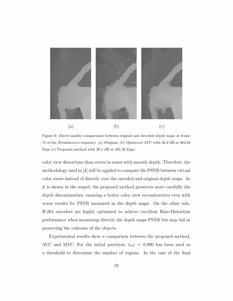
Fig. 6 presents examples of the original and decoded depth maps using

both Optimized AVC and the proposed method at similar bitrates. It can

be seen that the proposed method preserves better the contour information

and avoids the blurring/blocking artifacts that appear in the AVC or MVC

encoded images (Fig. 6.b) introducing only some small artifacts caused by

under-segmentation errors (Fig. 6.c).

In Fig. 6, the PSNR between a single frame of the original depth and

the Optimized AVC encoded depth is 32.4 dB while the same frame in the

proposed method achieves 28.1 dB (both at a similar bitrate of 484.24 and

481.32 kpbs for the entire MVD sequence respectively). However, depth maps

are not intended to be viewed directly but employed to generate virtual

views. For this reason, PSNR calculated on depth maps is not the best

measure for applications involving virtual-view reconstruction. Errors at the

border of depth discontinuities have a stronger contribution to reconstructed

17

(a) (b) (c)

Figure 6: Direct quality comparisons between original and decoded depth maps at frame

15 of the Breakdancers sequence. (a) Original, (b) Optimized AVC with 32.4 dB at 484.24

kbps (c) Proposed method with 28.1 dB at 481.32 kbps.

color view distortions than errors in zones with smooth depth. Therefore, the

methodology used in [4] will be applied to compute the PSNR between virtual

color views instead of directly over the encoded and original depth maps. As

it is shown in the sequel, the proposed method preserves more carefully the

depth discontinuities, ensuring a better color view reconstruction even with

worse results for PSNR measured in the depth maps. On the other side,

H.264 encoders are highly optimized to achieve excellent Rate-Distortion

performance when measuring directly the depth maps PSNR but may fail at

preserving the contours of the objects.

Experimental results show a comparison between the proposed method,

AVC and MVC. For the initial partition, tFP = 0.990 has been used as

a threshold to determine the number of regions. In the case of the final

18

partition, a value of tIP = 0.975 has been used. These two thresholds have

been determined empirically by testing different images and have been used

in all the results in the sequel. They result in approximately 500 regions for

Ballet and Breakdancers in the initial partition and 75/80 regions in the final

partition.

To encode the regions content, a second order orthobasis is employed and

each coefficient is represented using 8 bits. At each frame, all coefficients

for all regions are grouped and entropy coded using an adaptive arithmetic

codec.

The color views are encoded using Optimized AVC with quantization step

Q=32 and we assume they are available to the decoder. Using such a high

Q is a worst case scenario for our method as it decreases the quality of the

decoded color view partition. Fig. 7 shows the PSNR for virtual color views

along the 8 reference cameras for both Ballet and Breakdancers sequences

(obtained using the original and encoded depth maps). Nine virtual color

views are placed between each two reference cameras to estimate how the final

quality is affected by the distance from the reference cameras. As reported

in [4], PSNR values of virtual color views are significantly higher (around

35dB) than PSNR values measured directly between original and decoded

images. This is because both virtual views are generated using the same

color view; only the original and decoded depth map is changed, resulting in

more similar images and higher PSNR values.

Moreover, Fig. 7 shows a common trend of PSNRs measured in virtual

views, as the virtual view is located closer to one of the reference cameras,

the PSNR always increases even though the encoded depth map is the same

19

for all those virtual views. Thus, forming a characteristic “U” shape. Virtual

views in the middle of reference cameras need to make more use of the depth

map information than virtual views closer to one of the reference cameras.

Therefore, are more sensible to artifacts or errors in the decoded depth maps.

However, virtual views close to the reference cameras do not use depth map

information that much and the resulting virtual view quality is greater (thus,

increasing the PSNR). In the limit, a virtual view at the same place of the

reference camera will yield an infinite PSNR.

Table 1 shows the bitrates obtained encoding the depth maps with all

methods shown in Fig 7. The final bitrate is obtained by adding the bitrates

of the eight views. In the proposed method, the bitrate is composed of the

bits needed to allow the receiver building the final partition (list of differen-

tially encoded non-merging orders, number of regions in the initial and final

partitions) plus the bits needed to encode depth information for each region

(texture coefficients).

Table 1: Proposed method, AVC and MVC comparison (similar PSNR).

Ballet Breakdancers

kbps dB kbps dB

Proposed (Texture coeffs) 277.2 (57.6%) 285.08

Proposed (Non-merging orders) 204.12 (42.4%) 203.72

Proposed (Total) 481.32 37.39 488.8 38.37

AVC All I frames 2346.66 36.94 1317.42 38.53

AVC Optimized 813.51 37.02 648.03 38.07

MVC 843.62 37.17 632.04 38.28

20

0 1 2 3 4 5 6 732

34

36

38

40

42

44BALLET Sequence

Distance between Cameras

PSNR (d

b)

AVC (All I frames) Q=41AVC (Optimized) Q=41MVC Q=39Segmentation based method

0 1 2 3 4 5 6 734

36

38

40

42

44

46BREAKDANCER Sequence

Distance between Cameras

PSNR (d

b)

AVC (All I frames) Q=42AVC (Optimized) Q=42MVC Q=40Segmentation based method

Figure 7: Comparison between the proposed method, AVC and MVC for sequences Ballet

and Breakdancers at similar PSNR

As shown in Table 1, the total bitrate of our proposed method is much

lower than the All I frames AVC configuration. Even comparing with the

Optimized AVC or the MVC configurations, the resulting bitrate decreases

around 43% (for Ballet) and 22% (for Breakdancers) while keeping similar

PSNR values. Also, mean PSNR values in dBs for virtual color views are

shown in Table 1 for each coding configuration.

In Fig. 8 and Table 2 we can see an analogous comparison, this time for

similar bitrates. In this case, the All I frames AVC configuration obtains

a quality several dBs below the other two approaches and is not presented.

Gains up to 2.1 dB and 1.9 dB are achieved for the Ballet and Breakdancers

sequences respectively (1.4 dB and 0.8 dB in average). Experimental results

21

show that the more efficient MVC codec does not even outperform the AVC

codec proving that the higher R-D efficiency of the MVC does not directly

translate into higher PSNR values of the virtual color views.

0 1 2 3 4 5 6 730

32

34

36

38

40

42BALLET Sequence

Distance between Cameras

PSNR (d

b)

AVC (Optimized) Q=46MVC Q=44Segmentation based method

0 1 2 3 4 5 6 732

34

36

38

40

42

44BREAKDANCER Sequence

Distance between Cameras

PSNR (d

b)

AVC (Optimized) Q=46MVC Q=42Segmentation based method

Figure 8: Comparison between the proposed method, Optimized AVC and MVC for se-

quences Ballet and Breakdancers at similar bitrate.

4. Conclusion and future work

In this paper, we have presented a method for depth map compression

based on a novel approach. The main contribution of this paper is to ex-

ploit the redundancy between the color views and depth maps by using a

combination of decoded color view and depth partitions. Color partitions

are computed on the decoded views, which reduces the high cost commonly

associated to partition coding. Depth partitions in the decoder are built

22

Table 2: Proposed method, AVC and MVC comparison (similar bitrate).

Ballet Breakdancers

kbps dB kbps dB

Proposed (Texture coeffs) 277.2 (57.6%) 285.08

Proposed (Non-merging orders) 204.12 (42.4%) 203.72

Proposed (Total) 481.32 37.39 488.8 38.37

AVC Optimized 484.24 35.67 468.32 37.46

MVC 485.68 35.99 495.64 37.59

combining a decoded color view segmentation along with some overhead com-

plementary information from the original depth segmentation. Comparing

the final results with AVC and MVC, we achieve gains of more than 2 dB

for similar bitrates or reductions in bitrate around 40% for similar PSNR.

While the proposed method assumes the availability of the color views in the

decoder, we believe it is reasonable to expect so as depth maps are always

associated to color views to provide functionalities of free view point video

or 3DTV.

It is also important to note that the proposed method currently encodes

depth maps separately for each frame and neither temporal nor inter-view

prediction is performed so far. By exploiting these redundancies (both in

the final partition and in the depth information coding steps) we expect to

achieve even higher gains. Moreover, the use of a Binary Partition Tree

(BPT) [9] to represent the region-merging sequence will allow us to use a

rate-distortion approach to find an optimal segmentation, for instance by

selecting the best tIP and tFP thresholds or the optimal number of regions

23

in the initial and final partitions. Finally, alternative region-based texture

coding methods, such as DCT or partial wavelets, will be studied in order

to improve the depth information coding currently based on the orthobasis

approach.

References

[1] H. Ozaktas, L. Onural, Three-Dimensional Television: Capture, Trans-

mission, and Display, Springer, Heidelberg, 2007.

[2] A. Smolic, K. Muller, P. Merkle, C. Fehn, P. Kauff, P. Eisert, T. Wie-

gand, 3D video and free viewpoint video technologies, applications and

MPEG standards, in: IEEE International Conference on Multimedia

and Expo, Toronto, Canada, pp. 2161–2164.

[3] P. Merkle, A. Smolic, K. Muller, T. Wiegand, Efficient prediction struc-

tures for multiview video coding, IEEE Trans. on CSVT (2007) 1461–

1473.

[4] P. Merkle, Y. Morvan, A. Smolic, D. Farin, K. Muller, P. H. N. de With,

T. Wiegand, The effects of multiview depth video compression on mul-

tiview rendering, Image Commun. 24 (2009) 73–88.

[5] S.-U. Yoon, Y.-S. Ho, Multiple color and depth video coding using a

hierarchical representation, IEEE Trans. on CSVT 17 (2007) 1450–1460.

[6] M. Maitre, Y. Shinagawa, M. Do, Wavelet-based joint estimation and

encoding of depth-image-based representations for free-viewpoint ren-

dering, IEEE Trans. on Image Processing 17 (2008) 946–957.

24

[7] M. Maitre, M. N. Do, Shape-adaptive wavelet encoding of depth maps,

in: Picture Coding Symposium, volume 27, Chicago, USA, pp. 473–476.

[8] L. Torres, M. Kunt, Video Coding: The second generation approach,

Kluwer Academic Publishers, 1996.

[9] P. Salembier, L. Garrido, Binary partition tree as an efficient repre-

sentation for image processing, segmentation and information retrieval,

IEEE Trans. on IP 9 (2000) 561–576.

[10] V. Vilaplana, F. Marques, P. Salembier, Binary partition trees for object

detection, IEEE Trans. on Image Processing 17 (2008) 1–16.

[11] M. Gilge, T. Engelhardt, R. Mehlan, Coding of arbitrarily shaped image

segments based on a generalized orthogonal transform, Signal Process-

ing: Image Communication 1 (1989) 153–180.

[12] H. Zhang, J. E. Fritts, S. A. Goldman, Image segmentation evalua-

tion: A survey of unsupervised methods, Computer Vision and Image

Understanding 110 (2008) 260 – 280.

[13] S. Philipp-Foliguet, L. Guigues, Multi-scale criteria for the evaluation

of image segmentation algorithms, Journal of Multimedia 3 (2008).

[14] J.-P. Cocquerez, S. Philipp, Analyse dimages: filtrage et segmentation,

Masson, Paris, 1995.

[15] Interactive Visual Media Group of Microsoft Research,

MSR 3D video download, http://research.microsoft.com/en-

us/um/people/sbkang/3dvideodownload/, 2005.

25

[16] ITU-T, ISO/IEC JTC 1, Advanced video coding for generic audio-

visual services, ITU-T Recommendation H.264 and ISO/IEC 14496-10

(MPEG4-AVC), Version 4: July 2005.

26