MPRAMunich Personal RePEc Archive

Assessing Absolute and Relative PovertyTrends with Limited Data in Cape Verde

Diego Angel-Urdinola and Quentin Wodon

World Bank

January 2007

Online at http://mpra.ub.uni-muenchen.de/11111/MPRA Paper No. 11111, posted 16. October 2008 01:38 UTC

CHAPTER 5

Assessing Absolute and Relative Poverty Trends with

Limited Data in Cape Verde

By Diego Angel-Urdinola and Quentin Wodon23

Cape Verde shifted from a socialist to a capitalistic model in the late 1980s.This shift enabled the population to benefit from rapid economic growth, butconcerns have been expressed about a potential increase in inequality. Twohousehold surveys with consumption data implemented in 1988–89 and2001–02 provide information that can be used to assess the impact on welfareof this policy shift. Initial estimates based on these two surveys suggested thatthere had been an increase in poverty over time, but this was mainly due to theadoption of a relative measure of poverty and to comparability issues betweenthe surveys. The task of assessing the trends in poverty and inequality was alsomade more difficult because the unit level data of the first survey are not avail-able. For the period 1988–89, the only information at our disposal consists of anumber of tables on the distribution of income in the original report prepared15 years ago on that survey. This makes it necessary to estimate poverty andinequality using group data. In this paper, we use the Poverty module of SimSIPin order to obtain new poverty and inequality trends over time with group data.We find that despite an increase in inequality over time, and thereby an increasein relative measures of poverty, absolute poverty measures have been reduceddramatically thanks to rapid growth.

Cape Verde is a small country constituted by ten islands located 650 kilometers awayfrom the coast of Senegal and with an area of 4036 square kilometers. Out of theten islands, only nine are populated and more than half of the total population of

95

23. Diego Angel-Urdinola and Quentin Wodon are with the World Bank. This paper was prepared asa contribution to the poverty assessment for Cape Verde prepared by the World Bank (see World Bank2005; the previous poverty assessment dated back to 1994). The views expressed here are those of theauthors, and they do not necessarily represent those of the World Bank, its Executive Directors, or thecountries they represent.

434,625 people according to the 2002 census lives in the Island of Santigo. Due to the par-ticularities of the country’s Sahelian climate (dryness and lack of rain), only one tenth ofthe country’s soil is arable. Persistent periods of drought and a shortfall of water supplyfrom rivers and springs makes it difficult for the country to develop a stable agriculturalproduction, and even in the best rain seasons, agricultural production is able to supplyonly part of the population’s food requirements.

After independence in 1975, the economic model of Cape Verde relied on the govern-ment to assume a leading role of entrepreneurship in agriculture, industry, and services, giv-ing low importance to the private sector, and creating public enterprises within the keysectors of the economy. These strategies lead to deterioration in competitiveness, low lev-els of foreign direct investment, and poor overall economic performance. In 1988, the postindependence government adopted a new economic model with an outward orientedstrategy consisting on privatizing public enterprises and promoting trade liberalization.Government spending shifted rapidly into building economic and social infrastructure,leaving private investment to take the lead in some industries, especially light manufacturingand fisheries.

High unemployment rates in the late 1980s and inequalities between the islands led toa switch in government in 1991. The incoming government continued to decrease the roleof the state in the economy and set priorities towards improving education and reducingpoverty and unemployment. Also, new legislation and reforms, that still need to be refinedand implemented fully, were adopted on various aspects related to foreign investment, pri-vatization, and offshore banking services. The new government also pursued multilateral andbilateral donor assistance in order to improve services for human and capital infrastructure.

As a result of these reforms, remarkable growth has been achieved since the late 1980s.Between 1988 and 2002, real GDP grew, on average, at 6.4 percent and inflation was con-tained at an average rate of 3 percent per annum. Most of the growth was generated withinservices, where private sector activities increased dramatically as the state withdrew fromthe sector following reforms implemented throughout the 1990s. Construction and tradeare now the largest sectors of the economy. Together they constitute about 30 percent ofGDP (each accounts for about 15 percent of GDP). The fastest growing sectors within ser-vices, however, are hotel and restaurant services, transport, and communications. Thesesectors owe much of their growth to a large expansion in tourism. In 2001, tourist arrivalsincreased by 50 percent, and the number of visitors has been growing by 10 to 20 percent insubsequent years.

The objective of this paper is to assess the impact of the reforms on poverty, in the spe-cific sense of measuring the reduction in poverty that was achieved in parallel with theimplementation of reforms. The shift in policy enabled the population to benefit fromrapid economic growth, but concerns have been expressed about a potential increase ininequality. In order to assess the changes in poverty and inequality since the late 1980s, werely on two household surveys with consumption data implemented in 1988–89 and2001–02 (these are the IDRF surveys—Inquerito As Despensas E Receitas Familiares).Assessing the trends in poverty and inequality is however difficult because the unit leveldata of the first survey are not available. For the period 1988–89, the only information atour disposal consists of a number of tables on the distribution of income in the originalreport prepared 15 years ago on that survey. This makes it necessary to estimate povertyand inequality using group data, which is done using the Poverty module of SimSIP, a setof excel based tools for “Simulations for Social Indicators and Poverty.” The advantage of

96 World Bank Working Paper

using the SimSIP poverty module is that it enables the analyst to estimate poverty andinequality measures solely on the basis of grouped data. The next section provides ourmethodology. The second section describes the main results. We find that despite anincrease in inequality over time, poverty has been reduced dramatically thanks to rapidgrowth. A brief conclusion follows.

Methodology for Poverty Measurement

As noted in Coudouel and others (2002), in order to compute a poverty measure, threeingredients are needed. First, one has to select a relevant indicator of well-being. Second,one has to select a poverty line, that is, a threshold below which a given household or indi-vidual will be classified as poor. Finally, one has to select a poverty measure, which is usedfor reporting for the population as a whole or for a population subgroup only. In thispaper, we will rely on the Foster-Greer-Thorbecke (1984) class of poverty measures. Thegeneral formula for this class of poverty measures depends on a parameter α which takesa value of zero for the head count, one for the poverty gap, and two for the squared povertygap in the following expression:

The headcount index gives the share of the population or households in poverty. Thepoverty gap takes into account the distance separating the poor from the poverty line. Thesquared poverty gap places a higher weight on the poorest households in the sample.

Two poverty lines for the 2001–02 household survey were obtained using INE’smethodology. A household is considered as poor if its per capita consumption falls belowa relative poverty line equal to 60 percent of the median household consumption per capitain the 2001–02 survey. That is, the method consists in ranking all households according totheir per capita consumption, selecting the household at the 50th percentile of the distri-bution of household consumption, calculating a poverty line corresponding to 60 percentof the consumption level of that household, and considering all households with a lowerper capita consumption as poor. For extreme poverty, we use a poverty line equal to 40 per-cent of the median per capita consumption at the household level. Using these definitions,the poverty and extreme poverty lines used in this note are respectively CV$43,250 andCV$28,833 (Escudos) per capita per year. At the current exchange rate of approximately109 Escudos per U.S. dollar, this translates in poverty lines of about US$1.09 per day forpoverty, and US$0.73 per day for extreme poverty.

Note that if the definition had been based on the level of consumption of the medianindividual in the population as a whole (instead of the median household), the methodwould have resulted in lower poverty lines (and thereby lower poverty measures) as poorerhouseholds tend to be larger in household size, so that the household in which the medianindividual is located is poorer than the median household.

In the terminology of poverty measurement, the approach adopted by INE is a relativeapproach (because the poverty line is defined relatively, in comparison to the standard ofliving in the country). An absolute approach to poverty measurement would have proceededdifferently, by estimating a poverty line corresponding to the cost of basic food and non-food

Pn

z y

zi

i

q

αα

= −⎡⎣⎢

⎤⎦⎥=

∑11

1

( )

Growth and Poverty Reduction 97

needs. However, even though poverty was measured by INE in relative terms in 2001–02,we can still obtain absolute trends in poverty over time by adjusting the poverty lines esti-mated in 2001–02, to reflect the inflation observed between 1988–89 and 2001–02. We canalso obtain trends in relative poverty by applying the same method for estimating relativepoverty lines using the 1988–89 data. In this paper, we will provide both absolute and rela-tive poverty trends.

Following standard practice, the indicator of well-being is the per capita consumptionof the household obtained by aggregating all sources of consumption in the survey andwhen needed, imputing additional sources of consumption. The estimation of per capitaconsumption for the 2001–02 survey was done by INE. A key problem was to obtain sim-ilar values for 1988–89. Because we did not have access to the unit level data from that sur-vey, grouped data (mean values for different groups of households ranked by increasingconsumption levels) had to be used. We used tabulations provided in a report written closeto 15 years ago on poverty measurement with the 1988–89 survey. Yet the tabulations werenot available in an appropriate format. Instead of providing data on per capita consump-tion, the only estimates available were in terms of total household consumption, withoutinformation on the mean household size.

Specifically, the information we have at our disposal is provided in the first column ofTable 5.1. We know the share of total expenditure accruing to each of ten deciles of house-holds (each deciles comprises of ten percent of households). Given that we also have thetotal level of consumption in the survey, this enables us to compute the total level of con-sumption in each household decile. What we need to do is estimate the number of indi-viduals in each decile so that we can obtain an approximation of the level of per capitaconsumption by decile (by simply dividing household consumption by the estimatedhousehold size in each decile). Because we do not have access to the 1988–89 survey, weneed to work from the mean household sizes in 2001–02, and make a number of assump-

98 World Bank Working Paper

Percent of total Household Estimate of number Mean Consumption

consumption by consumption of individuals per capita by

household decile by decile by decile in 1988 household decile

Decile (1) (2) (3) (4)

1 2.0 224,129,24 34,542 6,489

2 3.0 336,193,86 33,200 10,126

3 4.0 448,258,48 31,769 14,110

4 6.0 672,387,72 32,042 20,985

5 6.0 672,387,72 31,749 21,178

6 8.0 896,516,96 31,112 28,816

7 10.0 1,120,646,20 30,407 36,855

8 13.0 1,456,840,06 27,414 53,142

9 17.0 1,905,098,54 25,489 74,741

10 31.0 3,474,003,22 19,137 181,536

Total 100.0 11,206,462,00 296,860 37,750

Table 5.1. Consumption Distribution in 1988/99 Based on Assumptions for Fertility Rates

Source: Authors using IDRF, 2001/02 and Inquérito as famílias, Cape Verde 1988–99.

tions in order to obtain estimates of the corresponding mean household sizes by house-hold decile for 1988–89, taking into account demographic trends.

As shown in Table 5.2, data from recent demographic and health-type surveys are avail-able on fertility rates in urban and rural areas for two periods of time: the period 1985–88,which precedes the first survey, and the period 1995–98, which precedes the second survey(INE, 1998). They show that fertility decreased faster in urban areas (from 5.24 to 3.14) thanin rural areas (from 6.40 to 4.85). The issue is to find a realistic way to relate these fertilityrates to expected changes in household size by consumption decile between both surveys.

Growth and Poverty Reduction 99

Fertility Rates

1995–1998 1985–1988

Total 4.030 5.950

Urban (U) 3.140 5.240

Rural (R) 4.850 6.400

U / (U + R) 0.393 0.450

Share of population Share of population Estimate for population

by household decile Share of population by household decile shares by household

(2001 data) adjustment factor (2001 data) adjusted decile in 1988/89 *

Decile (5) (6) (7) (8)

1 14.26 1.00 14.26 11.64

2 12.93 1.06 13.71 11.18

3 11.71 1.12 13.12 10.70

4 11.21 1.18 13.23 10.79

5 10.57 1.24 13.11 10.69

6 9.88 1.30 12.84 10.48

7 9.23 1.36 12.55 10.24

8 7.97 1.42 11.32 9.23

9 7.11 1.48 10.52 8.59

10 5.13 1.54 7.90 6.45

Total 100.0 - 122.55 100.00

Table 5.2. Using Fertility Data to Estimate Normalized Populations by Decile in 1988–89

Source: Authors using IDRF, 2001/02 and Inquérito as famílias, Cape Verde 1988–99.

Consider first the 2001–02 survey. The urban (U) fertility rate as a share to the sumof the urban and rural rates was 39.3 percent in 1995–98. We also know that householdsare roughly evenly divided between urban and rural areas. If we assume that the top halfof the distribution of households (the richer 50 percent) is somewhat representative ofthe urban areas because these are richer than rural areas, then we could conjecture on thebasis of the independent information on fertility rates that the population share in the tophalf of the distribution according to household deciles will be equal to 39.3 percent. Luckilyenough, this is what we observe in the data, as the actual population size in these fivedeciles is 39.3 percent.

Then, our assumption will be that for the previous survey, the population share in the topfive deciles should be roughly equal to 45.0 percent, which is the ratio of the fertility rate inurban areas divided by the sum of the fertility rates in urban and rural areas observed forthe period 1985–88. In order to obtain this cumulative population share of 45.0 percent, weneed to estimate “normalized population shares” by decile, denoted by NPopi

1988–89, foreach decile so that their sum for the top five deciles represent 45.0 percent of the totalpopulation, so that:

As fertility rates decrease over time, household sizes also decreases, so that for any givenhousehold decile, the mean household size should be smaller over time, but the speed ofthe reduction in fertility is likely to be strongest for the richest deciles (or for the urbanhouseholds, as noted above). We could assume for example that:

The problem with (4) is that if we simply multiply the population shares in 2001–02 in eachdecile by the parameters, we will have a sum of population shares above 100 percent in thesurvey as a whole. In order to get back to 100 percent as the sum of the population sharesin the various household deciles, we need to normalize the population shares as follows:

As shown in the bottom part of Table 5.2, the value of the parameter ρ that satisfies equa-tions (3) and (5) turns out to be 0.06. Using this parameter, we can compute the popula-tion or alternatively the household sizes in each decile in 1998–89. The results are given inthe third column of Table 5.1, which gives the estimated number of individuals in eachdecile, so that the per capita consumption can be computed in column 4. These are the val-ues that we will use for estimating poverty and inequality measures. Note that by recon-structing the household size and population in the 1988–89 survey, we find in Table 5.3

NPopi

NPop Ni i

1988 89 2001 021 1− −=+ −( ) × =

ρ, with

11 1

1005

2001 02

1

10

+ −( )( ) −

=∑ ρ j Popjj ( )

Pop Pop ii i i i

1988 89 2001 02 1 1− −= × = + −( )α α ρ,with .. ( )4

F

F FNPopU

U R

i

1985 88

1985 88 1985 88

1980 450−

− −+= =. 88 89

6

10

3−

=∑i

( )

F

F FPopU

U R

i

1995 98

1995 98 1995 98

20010 393−

− −+= =. −−

=∑ 02

6

10

2i

( )

100 World Bank Working Paper

Total Ratio of Consumption

Consumption per capita in survey

in National Total Total Expanded versus National

Accounts Population Consumption Sample Size Accounts

(1) (2) in Survey (3) (4) (5)

1988 19366000.0 328000.0 11206462.0 296860.0 0.6

2001 69934000.0 446000.0 46463000.0 470687.0 0.6

Table 5.3. Consumption in National Accounts vs. Consumption in Surveys

Source: Authors using 2001–02 and 1988–89 surveys. National Accounts data were provided by INE.

that the share of total consumption in the 1988–89 and 2001–02 surveys in proportion tototal private consumption as registered in the national accounts is very similar, at roughly60 percent, which gives us some confidence in comparing poverty and inequality estimatesobtained from both surveys.

Trend in Poverty

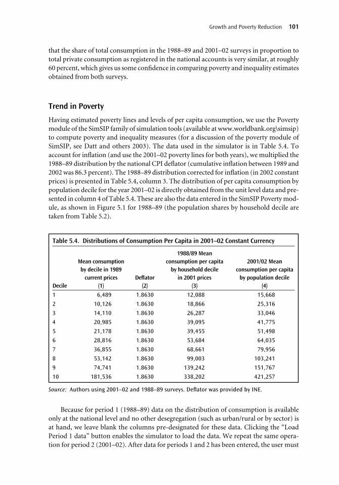
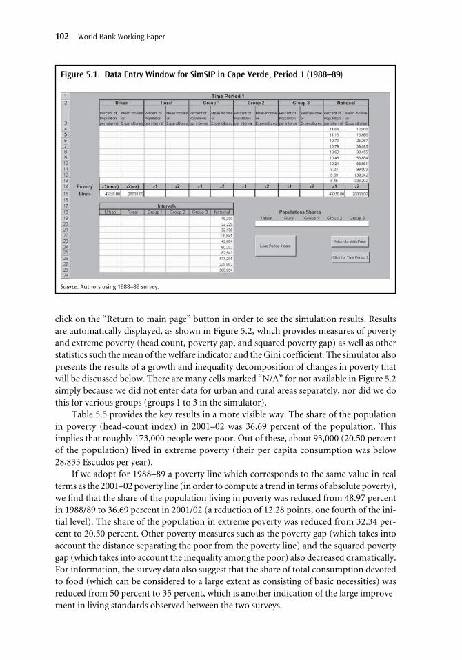
Having estimated poverty lines and levels of per capita consumption, we use the Povertymodule of the SimSIP family of simulation tools (available at www.worldbank.org\simsip)to compute poverty and inequality measures (for a discussion of the poverty module ofSimSIP, see Datt and others 2003). The data used in the simulator is in Table 5.4. Toaccount for inflation (and use the 2001–02 poverty lines for both years), we multiplied the1988–89 distribution by the national CPI deflator (cumulative inflation between 1989 and2002 was 86.3 percent). The 1988–89 distribution corrected for inflation (in 2002 constantprices) is presented in Table 5.4, column 3. The distribution of per capita consumption bypopulation decile for the year 2001–02 is directly obtained from the unit level data and pre-sented in column 4 of Table 5.4. These are also the data entered in the SimSIP Poverty mod-ule, as shown in Figure 5.1 for 1988–89 (the population shares by household decile aretaken from Table 5.2).

Growth and Poverty Reduction 101

1988/89 Mean

Mean consumption consumption per capita 2001/02 Mean

by decile in 1989 by household decile consumption per capita

current prices Deflator in 2001 prices by population decile

Decile (1) (2) (3) (4)

1 6,489 1.8630 12,088 15,668

2 10,126 1.8630 18,866 25,316

3 14,110 1.8630 26,287 33,046

4 20,985 1.8630 39,095 41,775

5 21,178 1.8630 39,455 51,498

6 28,816 1.8630 53,684 64,035

7 36,855 1.8630 68,661 79,956

8 53,142 1.8630 99,003 103,241

9 74,741 1.8630 139,242 151,767

10 181,536 1.8630 338,202 421,257

Table 5.4. Distributions of Consumption Per Capita in 2001–02 Constant Currency

Source: Authors using 2001–02 and 1988–89 surveys. Deflator was provided by INE.

Because for period 1 (1988–89) data on the distribution of consumption is availableonly at the national level and no other desegregation (such as urban/rural or by sector) isat hand, we leave blank the columns pre-designated for these data. Clicking the “LoadPeriod 1 data” button enables the simulator to load the data. We repeat the same opera-tion for period 2 (2001–02). After data for periods 1 and 2 has been entered, the user must

Source: Authors using 1988–89 survey.

click on the “Return to main page” button in order to see the simulation results. Resultsare automatically displayed, as shown in Figure 5.2, which provides measures of povertyand extreme poverty (head count, poverty gap, and squared poverty gap) as well as otherstatistics such the mean of the welfare indicator and the Gini coefficient. The simulator alsopresents the results of a growth and inequality decomposition of changes in poverty thatwill be discussed below. There are many cells marked “N/A” for not available in Figure 5.2simply because we did not enter data for urban and rural areas separately, nor did we dothis for various groups (groups 1 to 3 in the simulator).

Table 5.5 provides the key results in a more visible way. The share of the populationin poverty (head-count index) in 2001–02 was 36.69 percent of the population. Thisimplies that roughly 173,000 people were poor. Out of these, about 93,000 (20.50 percentof the population) lived in extreme poverty (their per capita consumption was below28,833 Escudos per year).

If we adopt for 1988–89 a poverty line which corresponds to the same value in realterms as the 2001–02 poverty line (in order to compute a trend in terms of absolute poverty),we find that the share of the population living in poverty was reduced from 48.97 percentin 1988/89 to 36.69 percent in 2001/02 (a reduction of 12.28 points, one fourth of the ini-tial level). The share of the population in extreme poverty was reduced from 32.34 per-cent to 20.50 percent. Other poverty measures such as the poverty gap (which takes intoaccount the distance separating the poor from the poverty line) and the squared povertygap (which takes into account the inequality among the poor) also decreased dramatically.For information, the survey data also suggest that the share of total consumption devotedto food (which can be considered to a large extent as consisting of basic necessities) wasreduced from 50 percent to 35 percent, which is another indication of the large improve-ment in living standards observed between the two surveys.

102 World Bank Working Paper

Figure 5.1. Data Entry Window for SimSIP in Cape Verde, Period 1 (1988–89)

Source: Authors using 2001–02 and 1988–99 surveys. Deflator was provided by INE.

Growth and Poverty Reduction 103

1998–99

Absolute poverty

(with 2001–02 1988–89 2001–02

relative poverty line) Relative poverty Relative poverty

Moderate Poverty

Head count 48.97% 31.15% 36.69%

Poverty Gap 21.48% 11.06% 13.59%

Squared poverty Gap 11.86% 5.02% 6.61%

Extreme Poverty

Head count 32.34% 17.32% 20.50%

Poverty Gap 11.70% 4.36% 5.96%

Squared poverty Gap 5.41% 1.40% 2.36%

Social Welfare

Mean consumption 70328 70328 98790

Gini index 50.17% 50.17% 52.83%

Mean*(1-Gini) 35044 35044 46600

Table 5.5. Trend in Poverty and Inequality Measures, Cape Verde 1998–99 to 2001–02

Source: Authors using SimSIP and 2001–02 and 1988–89 surveys.

Figure 5.2. SimSIP Results for Poverty Trends in Cape Verde, 1988–89 to 2001–02

If we adopt instead a relative poverty measurement approach for the 1988–89 survey,using an estimate of the median household per capita consumption of 46,570 Escudos, wefind that the corresponding poverty lines are respectively 27,941.77 Escudos for poverty,and 18,627.84 for extreme poverty. As shown in Table 5.5, we find that relative povertyincreased from 31.15 percent in 1988–89 to 36.69 percent in 2001–02, and relative extremepoverty increased similarly. This increase in relative poverty is due to an increase ininequality, as observed for example with the Gini index rising from 50.17 in 1988/89 to52.83 in 2001/02. Despite the increase in inequality, social welfare, as captured by the meanper capita consumption times one minus the Gini index, increased substantially, by abouta third versus the level in 1988–89.

The simulator also provides information on the changes in (absolute) poverty that aredue to growth and those that are due to the increase in inequality (Datt and Ravallion1992). Denoting by P(μt, Lt) the poverty measure corresponding to a mean income inperiod t of μt and a Lorenz curve Lt, the decomposition is:

The first component is the change in poverty that would have been observed if the Lorenzcurve had remained unchanged, while the second component is the change that would havebeen observed if mean income had not changed. The last component is a residual. As repro-duced in Table 5.6, without the increase in inequality, the reduction in the share of the pop-ulation in absolute poverty would have been larger (14.09 points for instead of 12.28 points).

ΔP P L P L P L P Lr r r r= ( )− ( )[ ]+ ( )− ( )[ ]+μ μ μ μ2 1 2 1, , , , RRr ( )6

104 World Bank Working Paper

Mod. poverty Extreme poverty

Growth Impact

Head count −14.09% −11.98%

Poverty Gap −8.39% −6.00%

Squared poverty Gap −5.59% −3.36%

Inequality Impact

Head count 3.15% 1.51%

Poverty Gap 1.10% 0.43%

Squared poverty Gap 0.57% 0.32%

Residual

Head count 1.34% 1.37%

Poverty Gap 0.59% 0.16%

Squared poverty Gap 0.24% 0.00%

Table 5.6. Growth-Inequality Decomposition of Changes in Poverty, 1998–99 to 2001–02

Source: Authors using SimSIP and 2001–02 and 1988–89 surveys.

The simulator also enables the user to predict future poverty based on growth assump-tions. Here, we report only simulations based on a national growth rate (simulations withdifferent growth rates for different sectors could also be provided). For example, if wewanted to be optimistic, we could first assume 13 years (from 2002 to 2015) of sustainedgrowth at 5 percent per year per capita. If there is no change in inequality, the impact will

be equivalent to multiplying the per capita consumption levels for all deciles by 1.89[because (1.05)13 = 1.885649]. The share of the population in (absolute) poverty wouldthen decrease from 36.69 percent to 13.11 percent, as shown in Figure 5.5 (the cells withN/A or #VALUE! in Figure 5.3 are again simply due to the fact that we did not enter in thesimulator separate data for urban and rural areas or by sector or “groups”).

Growth and Poverty Reduction 105

Figure 5.3. Future Poverty and Growth Simulation Results, Cape Verde

One question is whether the country is likely to achieve the Millennium DevelopmentGoal target or reducing poverty by half versus its 1990 level (for which the poverty mea-sures obtained in 1988–89 can be used as proxy). Given the progress achieved so far, theresults in Figure 5.4 suggest that if GDP continues to grow rapidly as in the previous years,poverty could easily be reduced by half in 2015 versus the 1990 level. Assuming that growthis evenly distributed among all individuals—assuming no future change in inequality, apossibly optimistic scenario given the mild increase in inequality in Cape Verde between1988/89 and 2001/02—under a constant growth rate in GDP per capita of 3, 4, and 5 per-cent per year, Cape Verde would be able to achieve the target of reducing poverty by halfset in the Millennium Development Goals by the years 2011, 2009, and 2008 respectively.Even if inequality were to continue to increase a bit, the target of reducing poverty by halfin 2015 would still be achieved under these growth assumptions.

Conclusion

Estimating trends in poverty in any country is often a difficult exercise. In Cape Verde, theexercise is made even more difficult than elsewhere because of comparability issuesbetween surveys, and because of the fact that the unit level data for the 1988/89 survey are

Source: Authors using SimSIP and 1988–89 surveys.

5.00

10.00

15.00

20.00

25.00

30.00

35.00

40.00

2002 2003 2004 2005 2006 2007 2008 2009 2010 2011 2012 2013 2014 2015

Po

vert

y In

cid

ence

Growth rate 5%Growth rate 4%Growth rate 3%Growth rate 5% (2002-2007), 3% (2007-2015)Millenium Dev. Goal

Source: Authors using SimSIP and the IDRF, 2001/02.

not available. At the time of the preparation of Cape Verde’s PRSP (Poverty ReductionStrategy Paper), concerns were raised regarding the fact that despite substantial growth inthe 1990s, poverty apparently had increased according to data from the household surveysimplemented in 1998–99 and 2001–02. This was a puzzling result, which put in doubt thecontribution of growth to poverty reduction, but was due to the use of relative povertycomparisons as well as issues of comparability between the two surveys.

The analysis provided in this paper confirms that there has been an increase in inequal-ity over time in the country, and thereby an increase in relative poverty, but it also suggeststhat absolute (as opposed to relative) poverty measures have been reduced substantially.Specifically, the strong economic performance observed in the 1990s (as a result of theimplementation of market-oriented reforms and political stability) contributed to reducethe share of the population in absolute poverty from 49 percent in 1988–89 to 37 percentin 2001–02. If GDP were to continue to grow rapidly, the country would easily be able toachieve the Millennium Development Goal of reducing poverty by half in 2015 versus the1990 level.

References

Coudouel, A., J. Hentschel, and Q. Wodon. 2002. “Poverty Measurement and Analysis.”In J. Klugman, editor, A Sourcebook for Poverty Reduction Strategies, Volume 1: CoreTechniques and Cross-Cutting Issues. Washington, D.C.: The World Bank.

Datt, G., K. Ramadas, D. van der Mensbrugghe, T. Walker, and Q. Wodon. 2003. “Pre-dicting the Effect of Aggregate Growth on Poverty.” In F. Bourguignon and L. Pereira

106 World Bank Working Paper

Figure 5.4. Simulations for Future Poverty Reduction Under Various Growth Scenarios

da Silva, editors, The Impact of Economic Policies on Poverty and Income Distribution:Evaluation Techniques and Tools. Washington, D.C.: The World Bank.

Datt, G., and M. Ravallion. 1992. “Growth and Redistribution Components of Changes inPoverty Measures: A Decomposition with Applications to Brazil and India in the 1980s.”Journal of Development Economics 38:275–95.

Foster, J. E., J. Greer, and E. Thorbecke. 1984. “A Class of Decomposable Poverty Indices.”Econometrica 52:761–66.

INE. 1998. Inquérito Demográfico de Saúde Reproductiva. Praia, Cape Verde.———. 2002. Carácterísticas Económicas de la Populaςao –Censo 2000. Praia, Cape Verde.World Bank. 1994. “Poverty in Cape Verde: A Summary Assessment and a Strategy for Its

Alleviation.” Report No. 13126-CV. Washington, D.C.———. 2005. “Cape Verde: Poverty Diagnostic.” Report No. 32826-CV. Washington, D.C.

Growth and Poverty Reduction 107