munich personal repec archive - mpra.ub.uni-muenchen.de · discrete choice models with...

MPRAMunich Personal RePEc Archive

Discrete choice models withmultiplicative error terms

Mogens Fosgerau and Michel Bierlaire

Technical University of Denmark

2009

Online at http://mpra.ub.uni-muenchen.de/42277/MPRA Paper No. 42277, posted 4. November 2012 15:08 UTC

http://mpra.ub.uni-muenchen.de/

http://mpra.ub.uni-muenchen.de/42277/

Discrete choice models with multiplicative

error terms

M. Fosgerau∗ M. Bierlaire†

September 15, 2008

2nd revised version, submitted for possible publication in Transportation

Research Part B.

∗Technical University of Denmark. Email: [email protected]†Ecole Polytechnique F�ed�erale de Lausanne, Transport and Mobility Laboratory, Sta-

tion 18, CH-1015 Lausanne, Switzerland. Email: michel.bierlaire@ep .ch

1

Abstract

The conditional indirect utility of many random utility maximiza-

tion (RUM) discrete choice models is speci�ed as a sum of an index

V depending on observables and an independent random term ε. In

general, the universe of RUM consistent models is much larger, even

�xing some speci�cation of V due to theoretical and practical consid-

erations. In this paper we explore an alternative RUM model where

the summation of V and ε is replaced by multiplication. This is con-

sistent with the notion that choice makers may sometimes evaluate

relative di�erences in V between alternatives rather than absolute dif-

ferences. We develop some properties of this type of model and show

that in several cases the change from an additive to a multiplicative

formulation, maintaining a speci�cation of V , may lead to a large im-

provement in �t, sometimes large than that gained from introducing

random coe�cients in V .

2

1 Introduction

Discrete choice models are widely used. They have a �rm theoretical foun-

dation in utility theory and can be adapted to a wide range of circum-

stances. Various very general and exible nonparametric discrete choice

models exist, but they tend not to be used so often in applied research for

various reasons. Instead a more limited range of models is employed based

on a set of often applied assumptions. The objective of the present paper is

to show how a small modi�cation of typical applied models may sometimes

lead to large improvements in �t without requiring additional parameters

to be estimated. The paper shows how these modi�ed models �t into the

general framework of random utility maximization and derives some basic

results about the modi�ed models that parallel established results for the

linear in parameters multinomial logit model and some of its generaliza-

tions. The results of this paper should thus be of interest for the applied

researcher.

McFadden and Train (2000), e.g., derive the general random utility max-

imization (RUM) discrete choice model from �rst principles. This model

speci�es the conditional indirect utility (CIU) associated with an alterna-

tive j as a function of observed and unobserved attributes (zj and εj) of

the alternative, and of observed and unobserved individual characteristics

(s and v), that is

U∗(zj, s, εj, v). (1)

Further speci�cation of this model is necessary before it can be applied to

data. In particular, we specify a subutility for each alternative j by

Vj = V(zj, s, v), (2)

which does not depend on unobserved characteristics of the alternative.

We proceed under the assumption that the researcher desires to specify V

up to a number of parameters to be estimated. Now, the CIU becomes

U∗(Vj, εj), (3)

which embodies the assumption that the variables zj, s and v may be sum-

marized by Vj. This is often called an index assumption where Vj is the

1

index. The corresponding choice model is

P(i|z, s) =

∫P(i|z, s, v)f(v)dv, (4)

where f(v) represents the distribution of v in the population, and

P(i|z, s, v) = Pr[U∗(Vi, εi) > U∗(Vj, εj) ∀j]. (5)

Most applications of these models have used a speci�cation with additive

independent error terms, that is

U∗(Vj, εj) = Vj + εj, (6)

where εj is independent of Vj. Some normalization is required for identi-

�cation, since any strictly increasing transformation of utility will lead to

identical observations of choice. It is hence necessary at least to �x the

location and scale of utility.1 This may be done by imposing constraints

on the distribution of the error term and on the speci�cation of the Vj.

Linear-in-parameter speci�cations of Vj ignoring unobserved individual

heterogeneity are commonly used, that is

Vj = V(zj, s, v) = β ′x(zj, s), (7)

so that (4){(5) simpli�es to

P(i|z, s) = Pr(β ′x(zi, s) + εi > β ′x(zj, s) + εj ∀j), (8)

and the mixing in (4) is avoided.

Operational models are based on speci�c assumptions about the dis-

tribution of εj. Assuming i.i.d. extreme value distributions leads to the

multinomial logit (MNL) model, which has been very successful due to

its computational and analytical tractability. Multivariate2 extreme value

1CITE Honore & Lewbel, Fosgerau & Nielsen some cases this is all that is required,

then something else is identi�ed and may be estimated consistently.2These models are called Generalized Extreme Value models by McFadden (1978).

However, the name GEV is also used for a family of univariate extreme value distributions

(see Jenkinson, 1955).

2

(MEV) models (McFadden, 1978) relax the assumption of mutual indepen-

dence. Mixtures of these models are derived to account for unobserved

heterogeneity, based on (4){(5). These models have gained popularity due

to their exibility (McFadden and Train, 2000), while retaining consistency

with RUM.

The applied researcher may have theoretical and practical reasons for

specifying V in certain ways. One concern is that the parameters of V

should have interpretations in terms of elasticities or marginal rates of sub-

stitution such as willingness-to-pay. In particular, the linear-in-parameters

speci�cation (6){(7) is very often used. In this paper we treat the speci�-

cation of V as �xed and focus on the speci�cation of the error structure.

We do not require V to be linear-in-parameters.

Given some speci�cation of V , the assumption of additive independent

errors (6) is not innocuous. It has strict implications for the range of

behavior that the model can describe. From (5), the additivity assumption

implies that choice probabilities are invariant with respect to addition of a

constant to all the Vs (Daly and Zachary, 1978). In contrast, multiplying

the Vs by a positive constant does a�ect the choice probabilities.

This may or may not be an adequate description of observed behavior.

It is quite conceivable that errors in (6) are heteroscedastic, violating the

independence assumption. One way that can happen is if choice makers

evaluate alternatives in terms of relative di�erences in V . Facing such is-

sues, if they are indeed detected, one may experiment with the speci�cation

of V . Sometimes another quite straight-forward solution may sometimes

apply, which is simply to replace the Vj's by logs. Then choice probabilities

will no longer be invariant with respect to addition of a constant to all the

Vj's, instead they will be invariant with respect to multiplication of all Vj's

by a positive constant.

We shall show that under appropriate circumstances, this modi�ed

model is still a RUM model. It may be considered a RUM model where

the assumption of additive independence of the error terms is replaced by

an assumption of multiplicative independence of the error terms. We are

thus exploring a second natural speci�cation of (3)

A number of authors have relaxed the assumption of iid errors by ex-

3

plicitly specifying the variance of the additive error term as a function of

observed and unobserved individual characteristics (Bhat, 1997; Swait and

Adamowicz, 2001; De Shazo and Fermo, 2002; Caussade et al., 2005; Kop-

pelman and Sethi, 2005; Train and Weeks, 2005). Our model modi�es the

assumption of iid errors in (6) by replacing the assumption by its multi-

plicative counterpart

U∗(Vj, εj) = Vjεj. (9)

If we are able to assume that the signs of Vj and εj are known, then we

are able to take logs without a�ecting choice probabilities, and the model

becomes an additive model, where Vj is replaced by lnVj.

The realization that there are alternatives to the additive speci�cation

of utility is not new. There is a recent literature about nonparametric

identi�cation of econometric models, which includes discrete choice models

with nonadditive unobservables. This literature is reviewed in Matzkin

(2007). (MICHEL INSERT REF: bibtex code included in this doc).

The multiplicative formulation is set out in the next section, Section 3

derives some properties of the multiplicative formulation, while Section 4

provides illustrative examples and Section 5 concludes.

2 Model formulation

Assume a general multiplicative utility function over a �nite set C of J

alternatives given by (9) where Vj < 0 is the systematic part of the utility

function, and εj > 0 is a random variable, independent of Vj.

We assume that the εj are i.i.d. across individuals. The sign restriction

on Vj is a natural assumption in many applications, for example when it

is de�ned as a generalized cost, that is, a linear combination of attributes

with positive values such as travel time and cost and parameters that are

a priori known to be negative.

The choice probabilities (5) under this model are given by

P(i|z, s, v) = Pr(Viεi ≥ Vjεj, ∀j). (10)

The multiplicative speci�cation is related to the classical speci�cation with

4

additive independent error terms, as can be seen from the following deriva-

tion. The logarithm is a strictly increasing function. Consequently,

P(i|z, s, v) = Pr(Viεi ≥ Vjεj, ∀j)= Pr(− ln(−Vi) − ln(εi) ≥ − ln(−Vj) − ln(εj), ∀j).

We de�ne

− ln(εj) = ξj/λ, (11)

where ξj are random variables, and λ > 0 is a scale parameter associated

with ξj. We obtain

P(i|z, s, v) = Pr( �Vi + ξi ≥ �Vj + ξj, j ∈ C)

= Pr(−λ ln(−Vi) + ξi ≥ −λ ln(−Vj) + ξj, j ∈ C).(12)

Consequently, this model can also be written in the random utility frame-

work with an additive speci�cation, where V is replaced by a logarithmic

form:�Vi = −λ ln(−Vi). (13)

In the linear formulation Vj = β ′xj with additive errors, identi�cation

requires that xj does not contain a variable that is constant across alter-

natives. An equivalent normalization in the multiplicative case is to �x a

parameter to a either 1 or -1, since multiplying V by a positive constant is

equivalent to adding a constant to ln(V). A useful practice is to normalize

the cost coe�cient (if present) to 1 so that other coe�cients can be readily

interpreted as willingness-to-pay indicators.

This speci�cation is fairly general and can be used for all the discrete

choice models discussed in the introduction. We are free to make assump-

tions regarding the error terms ξi and the parameters inside Vi can be

random. Thus we may obtain MNL, MEV and mixtures of MEV models.

For instance, a MNL speci�cation would be

P(i|z, s) =e−λ ln(−Vi)∑j∈C e−λ ln(−Vj)

=−V−λ

i∑j∈C −V−λ

j

. (14)

If random parameters are involved, it is necessary to ensure that P(Vi ≥0) = 0. The sign of a parameter can be restricted using, e.g., an exponential.

5

For instance, if β has a normal distribution then exp(β) is positive and log-

normal. For deterministic parameters one may specify bounds as part of

the estimation or transformations such as the exponential may be used to

restrict the sign.

The use of (12) provides an equivalent speci�cation with additive in-

dependent error terms, which �ts into the classical modeling framework,

involving MNL and MEV models, and mixtures of these. However, even

when the V 's are linear-in-parameters, the equivalent additive speci�ca-

tion (12) is nonlinear. Therefore, estimation routines must be used, that

are capable of handling this. The results presented in this paper have

been generated using the software package Biogeme (biogeme.epfl.ch;

Bierlaire, 2003; Bierlaire, 2005), which allows for the estimation of mix-

tures of MEV models, with nonlinear utility functions.

3 Model properties

We discuss now some basic properties of the model with multiplicative error

terms. As we have noted, we may simply reinterpret the model to have CIU

de�ned by �Vi +ξi, which is nonlinear when Vi is linear. This reformulation

yields identical choice probabilities but has additive error terms, such that

standard theory may be applied.

Distribution From (11), we derive the CDF of εi as

Fεi(x) = 1 − Fξi

(−λ ln x).

In the case where ξi is extreme value distributed, the CDF of ξi is

Fξi(x) = e−e−x

and, therefore,

Fεi(x) = 1 − e−xλ

.

This is a generalization of an exponential distribution (obtained with

λ = 1). We note that the exponential distribution is the maximum

entropy distribution among continuous distributions on the positive

6

half-axis of given mean, meaning that it embodies minimal informa-

tion in addition to the mean (that is to Vi) and positivity. Thus, it

is seems to be an appropriate choice for an unknown error term.

Elasticities The direct elasticity of alternative i with respect to an at-

tribute of the ith alternative xk is de�ned as

eik =∂P(i)

∂xk

xk

P(i)=

∂P(i)

∂Vi

∂Vi

∂xk

xk

P(i),

where ∂Vi/∂xk = βk if Vi is linear. We use (13) to obtain

eik =∂P(i)

∂ �Vi

∂ �Vi

∂Vi

∂Vi

∂xk

xk

P(i)= −

λ

Vi

∂P(i)

∂ �Vi

∂Vi

∂xk

xk

P(i)

where ∂P(i)/∂ �Vi may be derived from the corresponding additive

model. For instance, if the additive model is MNL, we have

∂P(i)

∂ �Vi

= P(i)(1 − P(i)),

and

eik = −λ

Vi

(1 − P(i))∂Vi

∂xk

xk.

Similarly, the cross-elasticity eijk of alternative i with respect to an

attribute xk of alternative j is given by

eik = −λ

Vj

∂P(i)

∂ �Vj

∂Vj

∂xk

xk

P(i)

where ∂P(i)/∂ �Vj can be derived from the corresponding additive model.

For instance, if the additive model is MNL, we have

∂P(i)

∂ �Vj

= −P(i)P(j),

and

eik =λ

Vi

P(j)∂Vj

∂xk

xk.

7

Trade-offs The trade-o�s are computed in the exact same way as for an

additive model, that is

∂Ui/∂xik

∂Ui/∂xi`

=∂Vi/∂xik

∂Vi/∂xi`

,

as ∂εi/∂xik = ∂εi/∂xi` = 0, because εi is independent of Vi.

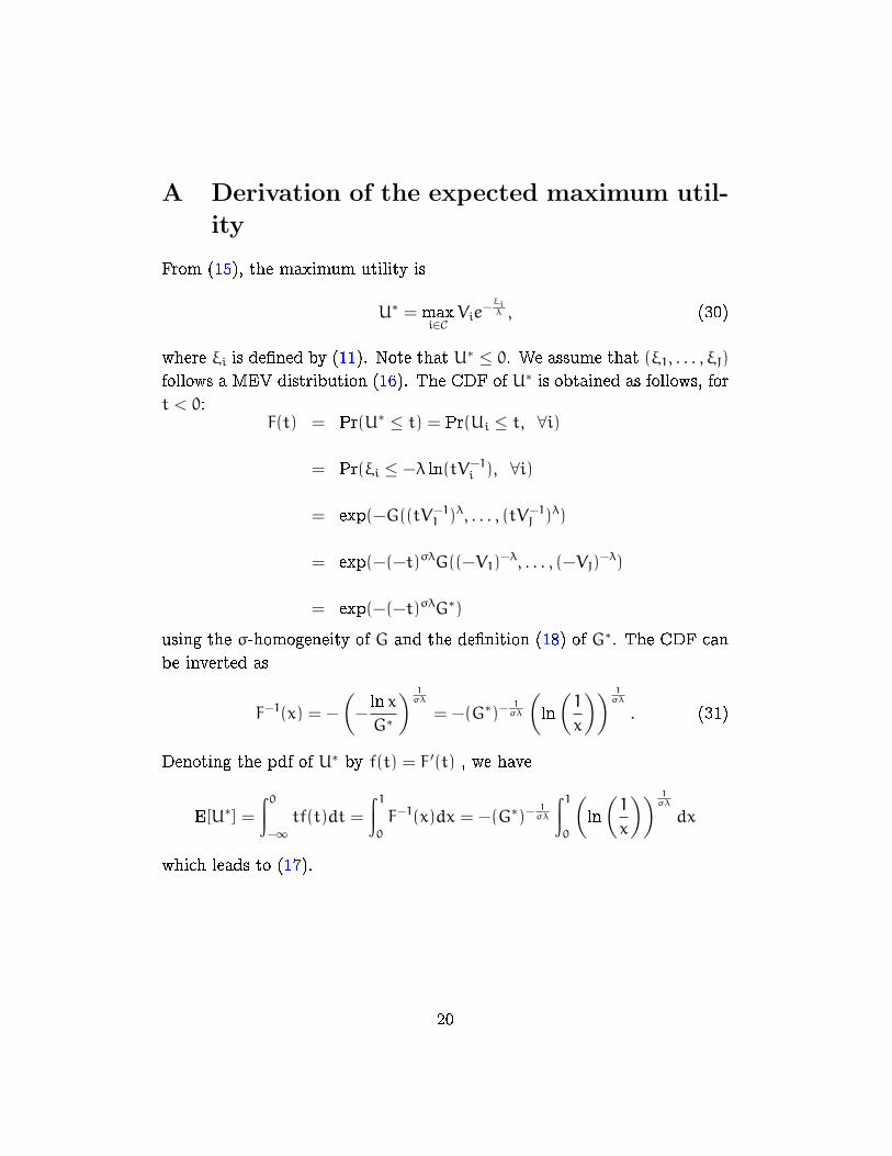
Expected maximum utility The maximum utility under the de�nition

of utility in (9) is

U∗ = maxi∈C

Ui = maxi∈C

Viεi = maxi∈C

Vie−

ξiλ , (15)

where ξi is de�ned by (11). We assume that (ξ1, . . . , ξJ) follows a

MEV distribution, that is

F(ξ1, . . . , ξJ) = e−G(e−ξ1 ,...,e−ξJ ), (16)

where G is a σ-homogeneous function with certain properties (see

McFadden, 1978 and Daly and Bierlaire, 2006 for details). Then the

expected maximum utility is given by (see derivation in Appendix

A):

E[U∗] = −(G∗)− 1σλ Γ

(1 +

1

σλ

), (17)

where

G∗ = G((−V1)−λ, . . . , (−VJ)

−λ), (18)

and Γ(·) is the gamma function.

We can compare this to the expected maximum utility if utility is

taken to be −λ ln(−Vi)+ξi. Using the well-known result (McFadden,

1978), the expected maximum utility is then 1σ(lnG∗ + γ).

It is thus apparent that for the same de�nition of V , the multiplicative

and the additive speci�cations of the model lead to quite di�erent ex-

pected utilities. But, essentially, the Vi enter the expected maximum

utility through G∗ in both expressions. Hence the marginal expected

maximum utility of a change to some Vi divided by the marginal

utility of income will be the same for either formulation.

8

Marshallian consumer surplus The Marshallian consumer surplus can

be derived in the context where −Vi, the negative of the subutility of

alternative i, is interpreted as a generalized cost. In this case, when

a small perturbation dVi is applied, the compensating variation is

simply −dVi if alternative i is chosen, and 0 otherwise. Therefore,

the compensating variation for a marginal change dVi in Vi is

−P(i)dVi, (19)

and the compensating variation for changing Vi from a to b is given

by

−

∫b

a

P(i)dVi. (20)

When P(i) is given by a classical MNL model, this integral leads to the

well-known logsum formula3. When P(i) is given by the model with

multiplicative error (like (14)), the integral does not have a closed

form in general and numerical integration must be performed4. We

refer the reader to Dagsvik and Karlstr�om (2005) for a discussion of

compensating variation in the context of discrete choice.

Heterogeneity of the scale of utility Assume that the utility can be de-

composed as

U∗(Vj, εj) = ~V(zj, s)µ(s, v)εj. (21)

That is, individual observed and unobserved heterogeneity v a�ects

only the scale of the utility. Combining (5) and (6) under the additive

speci�cation gives

P(i|z, s, v) = Pr( ~V(zi, s)µ(s, v) + εi > ~V(zj, s)µ(s, v) + εj ∀j), (22)

while combining (5) and (9) under the multiplicative speci�cation

gives

P(i|z, s, v) = Pr( ~V(zi, s)µ(s, v)εi > ~V(zj, s)µ(s, v)εj) ∀j), (23)

3Anders Karlstrom has helped us �nd references for this result. The earliest reference

we could �nd is Neuburger (1971)4Complicated closed form expressions can be derived for (14) with integer values of λ.

But λ is estimated and unlikely to be integer.

9

which simpli�es to

P(i|z, s, v) = Pr( ~V(zi, s)εi > ~V(zj, s)εj) ∀j). (24)

So the scale of utility is irrelevant for probabilities under the multi-

plicative formulation, also when the scale of utility is distributed in

the population.

4 Empirical applications

We analyze three stated choice panel data sets. We start with two data

sets for value of time estimation, from Denmark and Switzerland, where

the choice model is binomial. The third data set, a trinomial mode choice

in Switzerland, allows us to test the speci�cation with a nested logit model.

4.1 Value of time in Denmark

We utilize data from the Danish value-of-time study. We have selected an

experiment that involves several attributes in addition to travel time and

cost. We report the analysis for the train segment in detail, and provide a

summary for the bus and car driver segments. The experiment is a binary

route choice with unlabeled alternatives.

The �rst model is a simple logit model with linear-in-parameters subu-

tility functions. The attributes are the cost, in-vehicle time, number of

changes, headway, waiting time and access-egress time (ae).

The subutility function is de�ned as

Vi = λ( − cost +β1 ae +β2 changes

+ β3 headway +β4 inVehTime +β5 waiting ),(25)

where the cost coe�cient is normalized to -1 and the parameter λ is esti-

mated. The subutility function in log-form, used in the estimation software

for the multiplicative speci�cation, is de�ned as

Vi = −λ log( cost −β1 ae −β2 changes

− β3 headway −β4 inVehTime −β5 waiting) .(26)

10

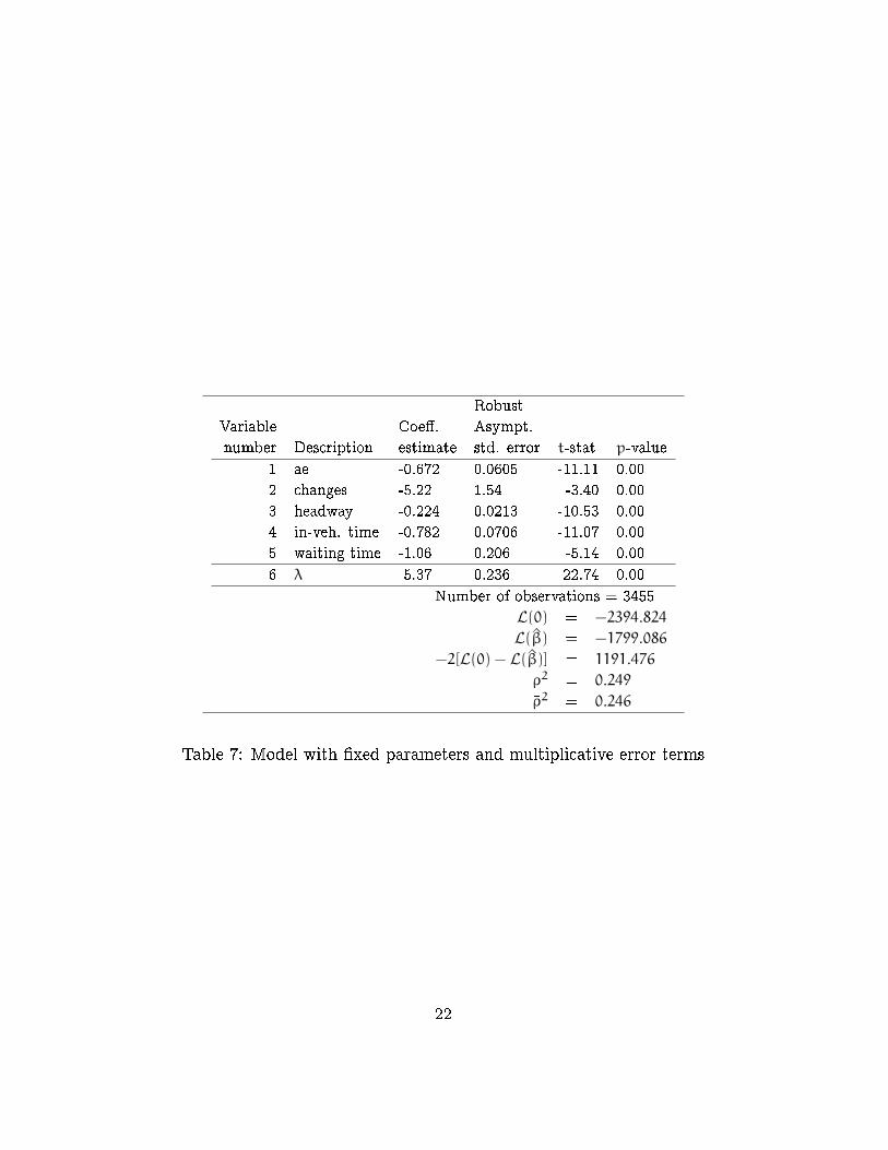
The estimation results are reported in Table 6 for the additive speci-

�cation and in Table 7 for the multiplicative speci�cation. We observe a

signi�cant improvement in the log-likelihood (171.76) for the multiplicative

speci�cation relative to the additive.

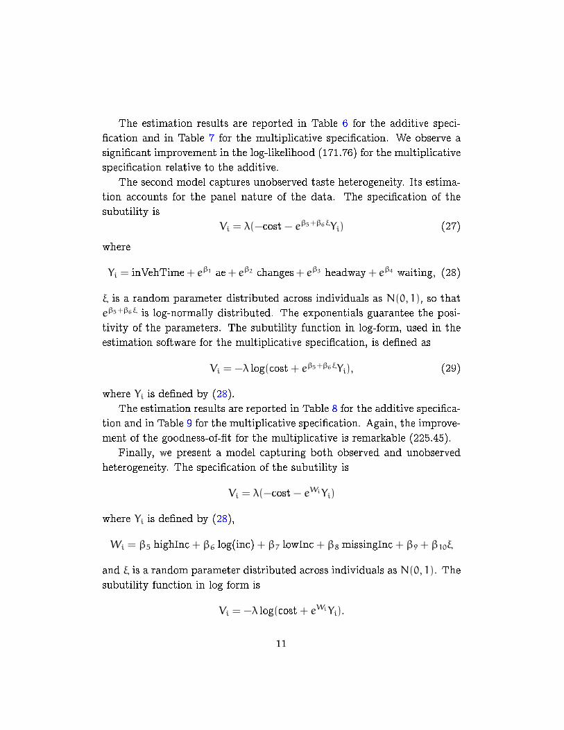
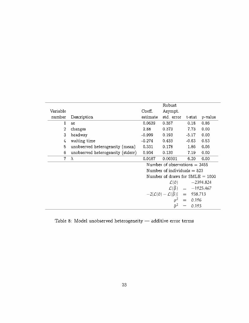
The second model captures unobserved taste heterogeneity. Its estima-

tion accounts for the panel nature of the data. The speci�cation of the

subutility is

Vi = λ(−cost− eβ5+β6ξYi) (27)

where

Yi = inVehTime+ eβ1 ae+ eβ2 changes+ eβ3 headway+ eβ4 waiting, (28)

ξ is a random parameter distributed across individuals as N(0, 1), so that

eβ5+β6ξ is log-normally distributed. The exponentials guarantee the posi-

tivity of the parameters. The subutility function in log-form, used in the

estimation software for the multiplicative speci�cation, is de�ned as

Vi = −λ log(cost+ eβ5+β6ξYi), (29)

where Yi is de�ned by (28).

The estimation results are reported in Table 8 for the additive speci�ca-

tion and in Table 9 for the multiplicative speci�cation. Again, the improve-

ment of the goodness-of-�t for the multiplicative is remarkable (225.45).

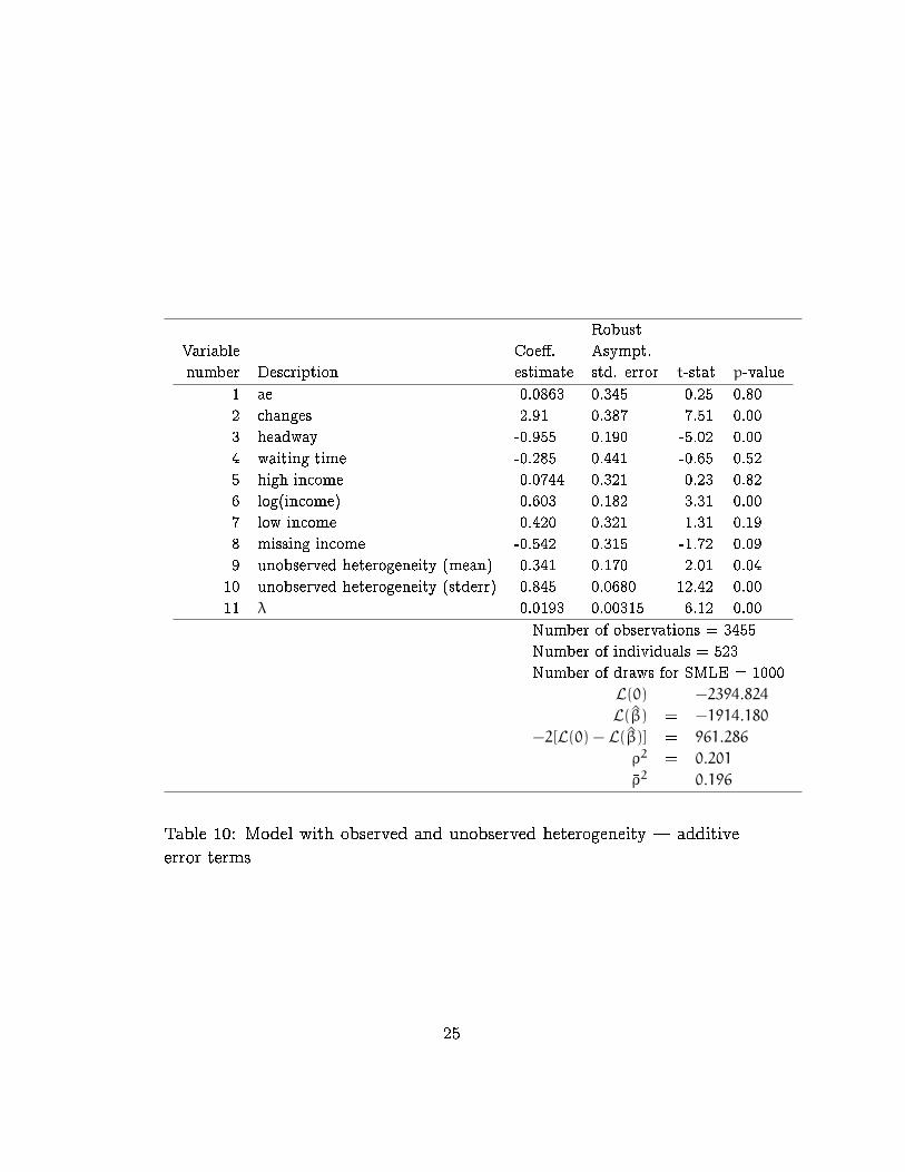
Finally, we present a model capturing both observed and unobserved

heterogeneity. The speci�cation of the subutility is

Vi = λ(−cost− eWiYi)

where Yi is de�ned by (28),

Wi = β5 highInc+ β6 log(inc)+ β7 lowInc+ β8 missingInc+ β9 + β10ξ

and ξ is a random parameter distributed across individuals as N(0, 1). The

subutility function in log form is

Vi = −λ log(cost+ eWiYi).

11

Number of observations 3455

Number of individuals 523

Model Additive Multiplicative Di�erence

1 -1970.85 -1799.09 171.76

2 -1924.39 -1698.94 225.45

3 -1914.12 -1674.67 239.45

Table 1: Log-likelihood of the models for the train data set

Number of observations: 7751

Number of individuals: 1148


1 -4255.55 -3958.35 297.2

2 -4134.56 -3817.49 317.07

3 -4124.21 -3804.9 319.31

Table 2: Log-likelihood of the models for the bus data set

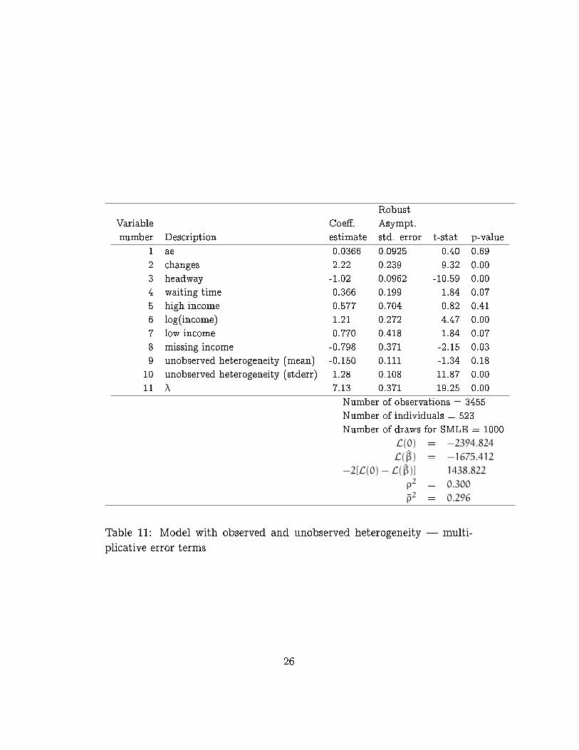
The estimation results are reported in Table 10 for the additive speci�-

cation and in Table 11 for the multiplicative speci�cation. We again obtain

a large improvement (239.45) of the goodness-of-�t for the multiplicative

model.

The log-likelihood of these three models are summarized in Table 1.

Similar models have been estimated on the bus and the car data set. The

summarized results are reported in Tables 2 and 3.

The multiplicative speci�cation signi�cantly and systematically outper-

forms the additive speci�cation in these examples. Actually, the multiplica-

tive model where taste heterogeneity is not modeled (model 1) �ts the data

much better than the additive model where both observed and unobserved

heterogeneity are modeled.

12

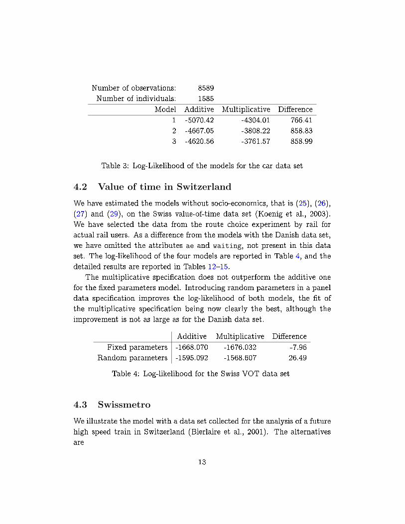
Number of observations: 8589

Number of individuals: 1585


1 -5070.42 -4304.01 766.41

2 -4667.05 -3808.22 858.83

3 -4620.56 -3761.57 858.99

Table 3: Log-Likelihood of the models for the car data set

4.2 Value of time in Switzerland

We have estimated the models without socio-economics, that is (25), (26),

(27) and (29), on the Swiss value-of-time data set (Koenig et al., 2003).

We have selected the data from the route choice experiment by rail for

actual rail users. As a di�erence from the models with the Danish data set,

we have omitted the attributes ae and waiting, not present in this data

set. The log-likelihood of the four models are reported in Table 4, and the

detailed results are reported in Tables 12{15.

The multiplicative speci�cation does not outperform the additive one

for the �xed parameters model. Introducing random parameters in a panel

data speci�cation improves the log-likelihood of both models, the �t of

the multiplicative speci�cation being now clearly the best, although the

improvement is not as large as for the Danish data set.

Additive Multiplicative Di�erence

Fixed parameters -1668.070 -1676.032 -7.96

Random parameters -1595.092 -1568.607 26.49

Table 4: Log-likelihood for the Swiss VOT data set

4.3 Swissmetro

We illustrate the model with a data set collected for the analysis of a future

high speed train in Switzerland (Bierlaire et al., 2001). The alternatives

are

13

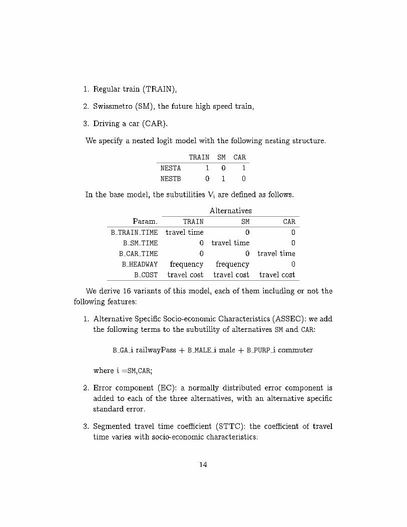
1. Regular train (TRAIN),

2. Swissmetro (SM), the future high speed train,

3. Driving a car (CAR).

We specify a nested logit model with the following nesting structure.

TRAIN SM CAR

NESTA 1 0 1

NESTB 0 1 0

In the base model, the subutilities Vi are de�ned as follows.

Alternatives

Param. TRAIN SM CAR

B TRAIN TIME travel time 0 0

B SM TIME 0 travel time 0

B CAR TIME 0 0 travel time

B HEADWAY frequency frequency 0

B COST travel cost travel cost travel cost

We derive 16 variants of this model, each of them including or not the

following features:

1. Alternative Speci�c Socio-economic Characteristics (ASSEC): we add

the following terms to the subutility of alternatives SM and CAR:

B GA i railwayPass + B MALE i male + B PURP i commuter

where i =SM,CAR;

2. Error component (EC): a normally distributed error component is

added to each of the three alternatives, with an alternative speci�c

standard error.

3. Segmented travel time coe�cient (STTC): the coe�cient of travel

time varies with socio-economic characteristics:

14

B SEGMENT TIME i = -exp(B i TIME + B GA i railwayPass +

B MALE i male + B PURP i commuter)

where i=fTRAIN,SM,CARg.

4. Random coe�cient (RC): the coe�cients for travel time and headway

are distributed, with a log-normal distribution.

For each variant, we have estimated both an additive and a multiplica-

tive speci�cation, using the panel dimension of the data when applicable.

The results are reported in Table 5.

RC EC STTC ASSEC Additive Multiplicative Di�erence

1 0 0 0 0 -5188.6 -4988.6 200.0

2 0 0 0 1 -4839.5 -4796.6 42.9

3 0 0 1 0 -4761.8 -4745.8 16.0

4 0 1 0 0 -3851.6 -3599.8 251.8

5 1 0 0 0 -3627.2 -3614.4 12.8

6 0 0 1 1 -4700.1 -4715.5 -15.4

7 0 1 0 1 -3688.5 -3532.6 155.9

8 0 1 1 0 -3574.8 -3872.1 -297.3

9 1 0 0 1 -3543.0 -3532.4 10.6

10 1 0 1 0 -3513.3 -3528.8 -15.5

11 1 1 0 0 -3617.4 -3590.0 27.3

12 0 1 1 1 -3545.4 -3508.1 37.2

13 1 0 1 1 -3497.2 -3519.6 -22.5

14 1 1 0 1 -3515.1 -3514.0 1.1

15 1 1 1 0 -3488.2 -3514.5 -26.2

16 1 1 1 1 -3465.9 -3497.2 -31.3

Table 5: Results for the 16 variants on the Swissmetro data

We observe that for simple models (1-5) the multiplicative speci�cation

outperforms the additive one. However, this is not necessarily true for

more complex models. Overall, the multiplicative speci�cation performs

better on 10 variants out of 16. We learn from this example that the

15

multiplicative (as expected) is not universally better, and should not be

systematically preferred. However, it is de�nitely worth testing it, as it has

a great potential for explaining the data better.

5 Concluding remarks

It seems to be a common perception that discrete choice models based on

random utility maximization must have additive independent error terms.

This is not the case, as we have discussed in this paper. It may happen

that for some data and some speci�cations of the subutility, it is more

appropriate to assume a multiplicative form. We have indicated how the

multiplicative form may be estimated with existing software.

A priori, for a given speci�cation of V , it is not possible to know whether

the multiplicative formulation will provide a better �t than the additive

formulation. However, in the majority of the cases we have looked at,

we �nd that the multiplicative formulation �ts the data better. In quite

a few cases, the improvement is very large, sometimes even larger than

the improvement gained from allowing for unobserved heterogeneity. We

emphasize that we are reporting the complete list of results that we have

obtained, whatever they turned out to be. The choice of applications was

motivated only by data availability. As both formulations are equally well

grounded in theory, we conclude that the choice between formulations is

an empirical question and should be answered by the ability of models to

�t data.

Of course, given some speci�cation of subutility, the universe of possi-

ble models is still larger than we have considered here. We have focused

on a multiplicative formulation as a clear cut alternative to the additive

formulation with an equally clear cut invariance property. For the multi-

plicative speci�cation, we are able to derive analogues to some theoretical

properties of the additive speci�cation. As an alternative one may rede�ne

the subutility by �Vj = −λln(−Vj) and use existing theory.

16

6 Acknowledgments

The authors like to thank Katrine Hjort for very competent research as-

sistance and Anders Karlstrom for comments on the paper. This work

has been initiated during the First Workshop on Applications of Discrete

Choice Models organized at Ecole Polytechnique F�ed�erale de Lausanne,

Switzerland, in September 2005. Mogens Fosgerau acknowledges support

from the Danish Social Science Research Council. Three anonymous re-

viewers provided us with very valuable comments on previous versions of

this article.

References

Bhat, C. R. (1997). Covariance heterogeneity in nested logit models: econo-

metric structure and application to intercity travel, Transportation

Research Part B: Methodological 31(1): 11{21.

Bierlaire, M. (2003). BIOGEME: a free package for the estimation of dis-

crete choice models, Proceedings of the 3rd Swiss Transportation

Research Conference, Ascona, Switzerland. www.strc.ch.

Bierlaire, M. (2005). An introduction to BIOGEME version 1.4. bio-

geme.ep .ch.

Bierlaire, M., Axhausen, K. and Abay, G. (2001). Acceptance of modal

innovation: the case of the Swissmetro, Proceedings of the 1st

Swiss Transportation Research Conference, Ascona, Switzerland.

www.strc.ch.

Caussade, S., Ort�uzar, J., Rizzi, L. I. and Hensher, D. A. (2005). Assessing

the in uence of design dimensions on stated choice experiment esti-

mates, Transportation Research Part B: Methodological 39(7): 621{

640.

17

Dagsvik, J. K. and Karlstr�om, A. (2005). Compensating variation and hick-

sian choice probabilities in random utility models that are nonlinear

in income, Review of Economic Studies 72(1): 57{76.

Daly, A. and Bierlaire, M. (2006). A general and operational representation

of generalised extreme value models, Transportation Research Part

B: Methodological 40(4): 285{305.

Daly, A. J. and Zachary, S. (1978). Improved multiple choice, in D. A.

Hensher and M. Q. Dalvi (eds), Determinants of travel demand,

Saxon House, Sussex.

De Borger, B. and Fosgerau, M. (forthcoming). The trade-o� between

money and travel time: A test of the theory of reference-dependent

preferences, Journal of Urban Economics .

De Shazo, J. and Fermo, G. (2002). Designing choice sets for stated prefer-

ence methods: the e�ects of complexity on choice consistency, Journal

of Environmental Economics and Management 44: 123{143.

Fosgerau, M. (2006). Investigating the distribution of the value of travel

time savings, Transportation Research Part B: Methodological

40(8): 688{707.

Fosgerau, M. (2007). Using nonparametrics to specify a model to measure

the value of travel time, Transportation Research Part A 41(9): 842{

856.

Hanemann, W. M. (1984). Discrete/continuous models of consumer de-

mand, Econometrica 52(3): 541{561.

Jenkinson, A. F. (1955). Frequency distribution of the annual maximum

(or minimum) values of meteorological elements, Quarterly journal

of the Royal Meteorological Society 81: 158{171.

Koenig, A., Abay, G. and Axhausen, K. (2003). Time is money:

the valuation of travel time savings in switzerland, Proceed-

ings of the 3rd Swiss Transportation Research Conference.

http://www.strc.ch/Paper/Koenig.pdf.

18

Koppelman, F. and Sethi, V. (2005). Incorporating variance and covariance

heterogeneity in the generalized nested logit model: an application to

modeling long distance travel choice behavior, Transportation Re-

search Part B: Methodological 39(9): 825{853.

McFadden, D. and Train, K. (2000). Mixed MNL models for discrete re-

sponse, Journal of Applied Econometrics 15(5): 447{470.

McFadden, D. (1978). Modelling the choice of residential location, in A.

Karlquist et al. (ed.), Spatial interaction theory and residential lo-

cation, North-Holland, Amsterdam, pp. 75{96.

Neuburger, H. (1971). User bene�t in the evaluation of transport and land

use plans, Journal of Transport Economics and Policy 5: 52{75.

Swait, J. and Adamowicz, W. (2001). Choice environment, market com-

plexity, and consumer behavior: a theoretical and empirical ap-

proach for incorporating decision complexity into models of consumer

choice, Organizational Behavior and Human Decision Processes

86(2): 141{167.

Train, K. and Weeks, M. (2005). Discrete choice models in preference

space and willingness-to-pay space, in R. Scarpa and A. Alberini

(eds), Applications of simulation methods in environmental and

resource economics, The Economics of Non-Market Goods and Re-

sources, Springer, pp. 1{16.

19

A Derivation of the expected maximum util-

ity

From (15), the maximum utility is

U∗ = maxi∈C

Vie−

ξiλ , (30)

where ξi is de�ned by (11). Note that U∗ ≤ 0. We assume that (ξ1, . . . , ξJ)

follows a MEV distribution (16). The CDF of U∗ is obtained as follows, for

t < 0:F(t) = Pr(U∗ ≤ t) = Pr(Ui ≤ t, ∀i)

= Pr(ξi ≤ −λ ln(tV−1i ), ∀i)

= exp(−G((tV−11 )λ, . . . , (tV−1

J )λ)

= exp(−(−t)σλG((−V1)−λ, . . . , (−VJ)

−λ)

= exp(−(−t)σλG∗)

using the σ-homogeneity of G and the de�nition (18) of G∗. The CDF can

be inverted as

F−1(x) = −

(−ln x

G∗

) 1σλ

= −(G∗)− 1σλ

(ln

(1

x

)) 1σλ

. (31)

Denoting the pdf of U∗ by f(t) = F ′(t) , we have

E[U∗] =

∫ 0

−∞ tf(t)dt =

∫ 1

0

F−1(x)dx = −(G∗)− 1σλ

∫ 1

0

(ln

(1

x

)) 1σλ

dx

which leads to (17).

20

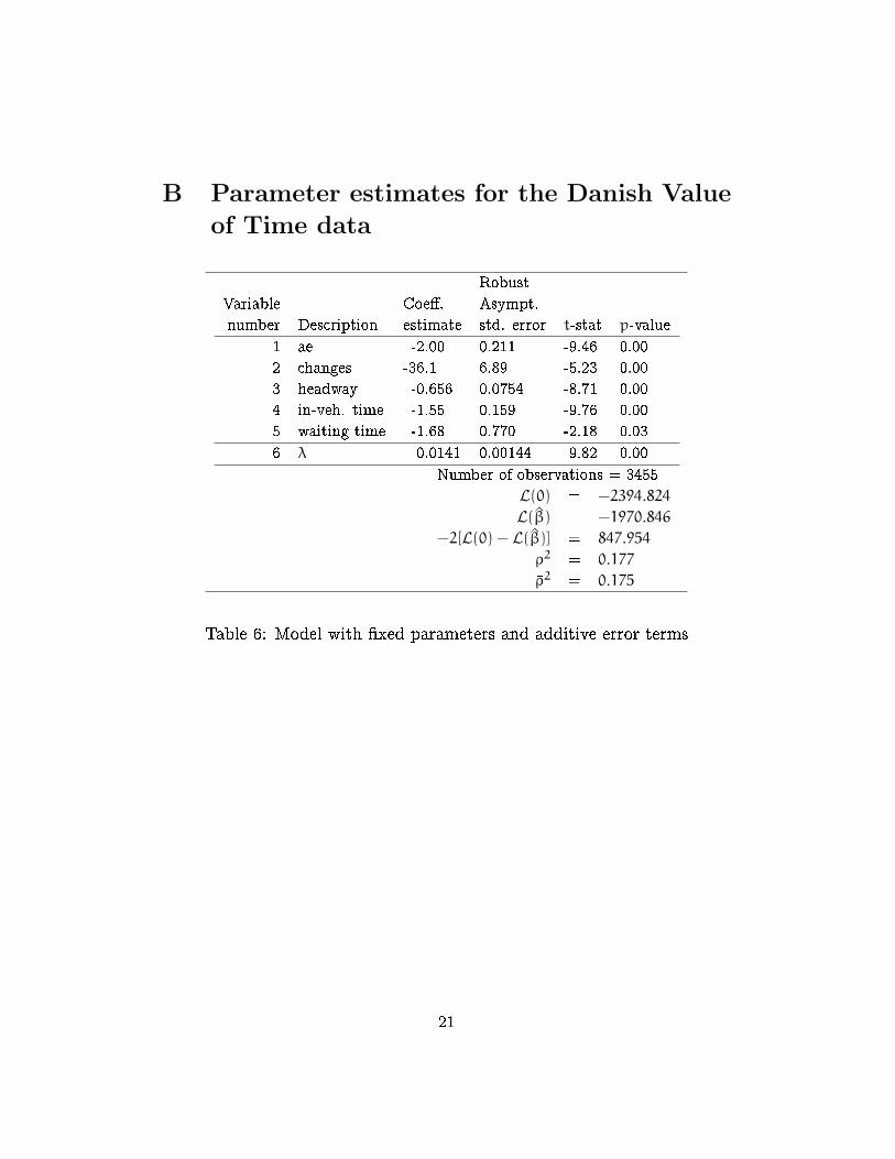
B Parameter estimates for the Danish Value

of Time data

Robust

Variable Coe�. Asympt.

number Description estimate std. error t-stat p-value

1 ae -2.00 0.211 -9.46 0.00

2 changes -36.1 6.89 -5.23 0.00

3 headway -0.656 0.0754 -8.71 0.00

4 in-veh. time -1.55 0.159 -9.76 0.00

5 waiting time -1.68 0.770 -2.18 0.03

6 λ 0.0141 0.00144 9.82 0.00

Number of observations = 3455

L(0) = −2394.824

L(β̂) = −1970.846

−2[L(0) − L(β̂)] = 847.954

ρ2 = 0.177

�ρ2 = 0.175

Table 6: Model with �xed parameters and additive error terms

21

Robust



1 ae -0.672 0.0605 -11.11 0.00

2 changes -5.22 1.54 -3.40 0.00

3 headway -0.224 0.0213 -10.53 0.00

4 in-veh. time -0.782 0.0706 -11.07 0.00

5 waiting time -1.06 0.206 -5.14 0.00

6 λ 5.37 0.236 22.74 0.00


L(0) = −2394.824

L(β̂) = −1799.086

−2[L(0) − L(β̂)] = 1191.476

ρ2 = 0.249

�ρ2 = 0.246

Table 7: Model with �xed parameters and multiplicative error terms

22

Robust



1 ae 0.0639 0.357 0.18 0.86

2 changes 2.88 0.373 7.73 0.00

3 headway -0.999 0.193 -5.17 0.00

4 waiting time -0.274 0.433 -0.63 0.53

5 unobserved heterogeneity (mean) 0.331 0.178 1.86 0.06

6 unobserved heterogeneity (stderr) 0.934 0.130 7.19 0.00

7 λ 0.0187 0.00301 6.20 0.00


Number of individuals = 523

Number of draws for SMLE = 1000

L(0) = −2394.824

L(β̂) = −1925.467

−2[L(0) − L(β̂)] = 938.713

ρ2 = 0.196

�ρ2 = 0.193

Table 8: Model unobserved heterogeneity | additive error terms

23

Robust



1 ae 0.0424 0.0946 0.45 0.65

2 changes 2.24 0.239 9.38 0.00

3 headway -1.03 0.0983 -10.48 0.00

4 waiting time 0.355 0.207 1.72 0.09

5 unobserved heterogeneity (mean) -0.252 0.106 -2.38 0.02


7 λ 7.04 0.370 19.02 0.00




L(0) = −2394.824

L(β̂) = −1700.060

−2[L(0) − L(β̂)] = 1389.528

ρ2 = 0.290

�ρ2 = 0.287

Table 9: Model with unobserved heterogeneity |multiplicative error terms

24

Robust



1 ae 0.0863 0.345 0.25 0.80

2 changes 2.91 0.387 7.51 0.00

3 headway -0.955 0.190 -5.02 0.00

4 waiting time -0.285 0.441 -0.65 0.52

5 high income 0.0744 0.321 0.23 0.82

6 log(income) 0.603 0.182 3.31 0.00

7 low income 0.420 0.321 1.31 0.19

8 missing income -0.542 0.315 -1.72 0.09

9 unobserved heterogeneity (mean) 0.341 0.170 2.01 0.04


11 λ 0.0193 0.00315 6.12 0.00




L(0) = −2394.824

L(β̂) = −1914.180

−2[L(0) − L(β̂)] = 961.286

ρ2 = 0.201

�ρ2 = 0.196

Table 10: Model with observed and unobserved heterogeneity | additive

error terms

25

Robust



1 ae 0.0366 0.0925 0.40 0.69

2 changes 2.22 0.239 9.32 0.00

3 headway -1.02 0.0962 -10.59 0.00

4 waiting time 0.366 0.199 1.84 0.07

5 high income 0.577 0.704 0.82 0.41

6 log(income) 1.21 0.272 4.47 0.00

7 low income 0.770 0.418 1.84 0.07

8 missing income -0.798 0.371 -2.15 0.03



11 λ 7.13 0.371 19.25 0.00




L(0) = −2394.824

L(β̂) = −1675.412

−2[L(0) − L(β̂)] = 1438.822

ρ2 = 0.300

�ρ2 = 0.296

Table 11: Model with observed and unobserved heterogeneity | multi-

plicative error terms

26

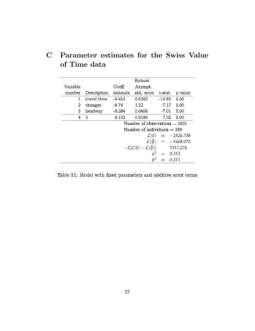
C Parameter estimates for the Swiss Value

of Time data

Robust



1 travel time -0.453 0.0383 -11.82 0.00

2 changes -8.74 1.22 -7.17 0.00

3 headway -0.284 0.0406 -7.01 0.00

4 λ 0.132 0.0188 7.02 0.00



L(0) = −2426.708

L(β̂) = −1668.070

−2[L(0) − L(β̂)] = 1517.276

ρ2 = 0.313

�ρ2 = 0.311

Table 12: Model with �xed parameters and additive error terms

27

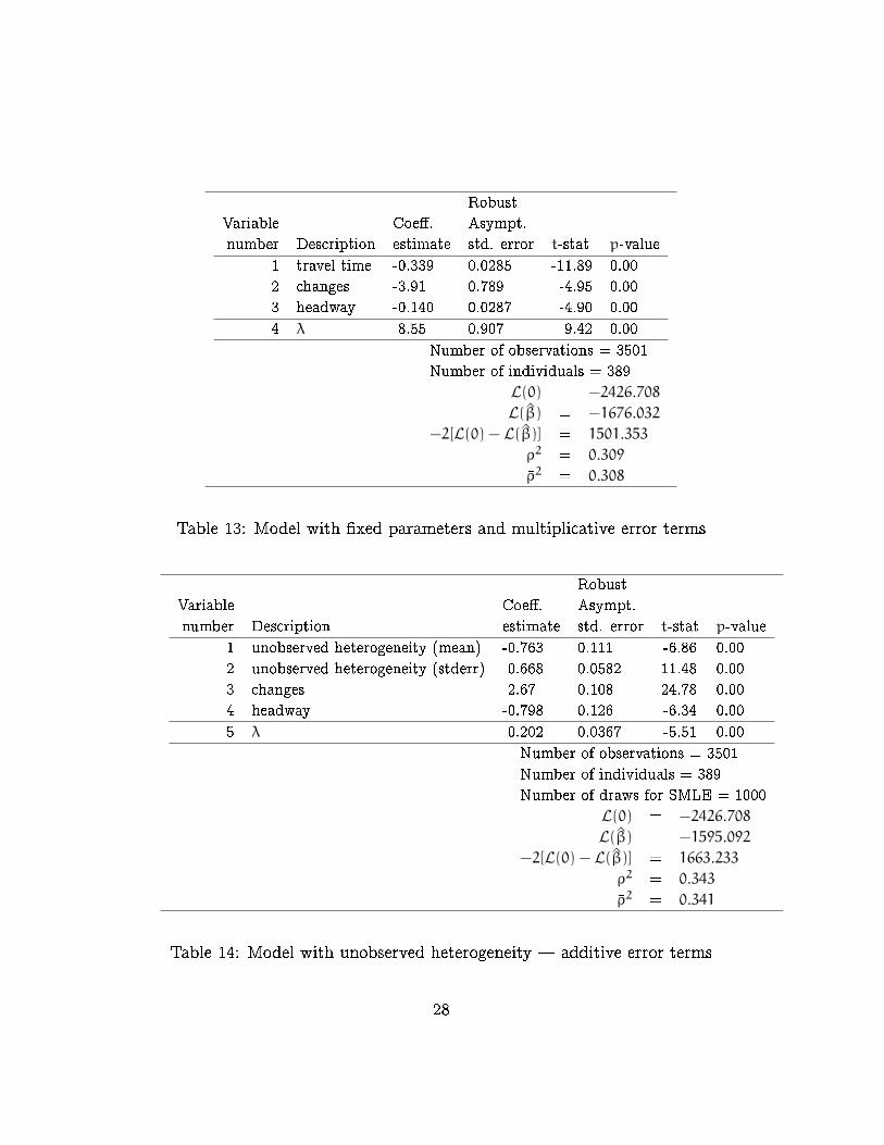
Robust



1 travel time -0.339 0.0285 -11.89 0.00

2 changes -3.91 0.789 -4.95 0.00

3 headway -0.140 0.0287 -4.90 0.00

4 λ 8.55 0.907 9.42 0.00



L(0) = −2426.708

L(β̂) = −1676.032

−2[L(0) − L(β̂)] = 1501.353

ρ2 = 0.309

�ρ2 = 0.308

Table 13: Model with �xed parameters and multiplicative error terms

Robust





3 changes 2.67 0.108 24.78 0.00

4 headway -0.798 0.126 -6.34 0.00

5 λ 0.202 0.0367 -5.51 0.00




L(0) = −2426.708

L(β̂) = −1595.092

−2[L(0) − L(β̂)] = 1663.233

ρ2 = 0.343

�ρ2 = 0.341

Table 14: Model with unobserved heterogeneity | additive error terms

28

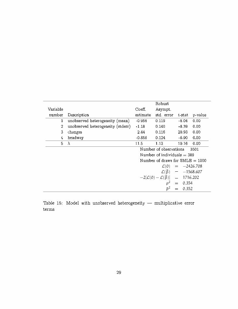
Robust




2 unobserved heterogeneity (stderr) -1.18 0.140 -8.39 0.00

3 changes 2.44 0.116 20.93 0.00

4 headway -0.856 0.124 -6.90 0.00

5 λ 11.5 1.13 10.16 0.00




L(0) = −2426.708

L(β̂) = −1568.607

−2[L(0) − L(β̂)] = 1716.202

ρ2 = 0.354

�ρ2 = 0.352

Table 15: Model with unobserved heterogeneity | multiplicative error

terms

29

munich personal repec archive - mpra.ub.uni-muenchen.de · discrete choice models with...

Documents