Munich Personal RePEc Archive

Impacts of Donald Trump’s TariffIncrease against China on GlobalEconomy: Global Trade Analysis Project(GTAP) Model

Alim Rosyadi, Saiful and Widodo, Tri

Economics Department, Fauclty of Economics and Business, Gadjah

Mada University

29 May 2017

Online at https://mpra.ub.uni-muenchen.de/79493/

MPRA Paper No. 79493, posted 02 Jun 2017 19:49 UTC

1

Impacts of Donald Trump’s Tariff Increase against China on Global

Economy: Global Trade Analysis Project (GTAP) Model

by:

Saiful Alim Rosyadi

Undergraduate Program, Economics Department, Faculty of Economics and Business,

Gadjah Mada University, Indonesia

and

Tri Widodo

Economics Department, Faculty of Economics and Business, Gadjah Mada University, Indonesia

Current Mailing Address: Faculty of Economics and Business, Gadjah Mada University, Jl. Humaniora No.

1, Bulaksumur, Yogyakarta 55281, Indonesia. Phone: 62 (274) 548510; fax. 62 (274) 563 212. E-mail address:

kociwid@yahoo.com.

2

Impacts of Donald Trump’s Tariff Increase against China on Global

Economy: Global Trade Analysis Project (GTAP) Model

Abstract

This paper aims to analyze the possible impacts of the US import tariff against

China on global economy. The GTAP model is implemented. The simulation

scenarios depicted short-run effects of full-protection and manufacturing protection

with appropriate retaliation response from China. On global level, the policy was

projected to lead to decline in GDP, terms-of-trade, and welfare; and increase in

trade balance for United States and China. Trade diversion phenomena would occur,

predicting steep decline in bilateral trade between the two countries and increasing

export towards their third trading partners.

Keywords: Donald Trump, Tariff Increase, GTAP Model

JEL: F13, F17

1. Introduction

The United States’ presidential election on November 8, 2016 had elected Donald

J. Trump as its 45th president. He was later sworn into the office on January 20,

2017. The world was taken by surprise considering that Trump’s campaign included

several controversial trade protectionism plans. These promises were pledged in

conjunction with his campaign to reclaim the so-called “American Economic

Independence”. Below are some of his plans, as delivered in his speech on June 28,

2016 at Alumisource Factory, Monessen, Pennsylvania (Trump, 2016).

1. Withdrawal of United States from Trans-Pacific Partnership

2. Appointments of trade negotiators to fight for American workers

3. Direction of all appropriate agencies to end foreign trade abuses that harm

United States’ labor force. 4. Renegotiation of NAFTA terms of agreement to favor United States’ labor

force

5. Labeling China as currency manipulator

6. Bringing trade cases against China’s unfair subsidy behavior to WTO.

3

7. Remediation of trade dispute with China, including possibility of tariff

imposition against Chinese imports.

In the same speech, he further claimed that “NAFTA was the worst trade deals

in history, and China’s entrance into World Trade Organization has enabled the

greatest jobs theft in history. [..] Almost half of our entire manufacturing trade

deficit in goods with the world is the result of trade with China” (Trump, 2016).

United States’ various free-trade deals “like the North American Free-Trade

Agreement (NAFTA) and China’s accession to the World Trade Organization

(WTO)” were claimed to “have destroyed American jobs and created American

losers” (The Economist, 2016).

Regarding the last campaign promise outlined above, Donald Trump mentioned

his planned rate of import tariff earlier on January 3, 2016 in a release by The New

York Times which goes as follows.

“In the editorial board meeting, which was held Tuesday, Mr. Trump

said that the relationship with China needs to be restructured. “The only power that we have with China,” Mr. Trump said, “is massive trade.” “I would tax China on products coming in,” Mr. Trump said. “I would do a tariff, yes – and they do it to us.” (….) “I would do a tax. And the tax, let me tell you what the tax should be… the tax should be 45 percent,” Mr. Trump said.” (Haberman, 2016)

However, the amount of rate increase has not been finalized or drafted as a

proper policy proposal. In a later occasion on April, 2016, he explained further that

“It doesn’t have to be 45; it could be less. But it has to be something because our

country and our trade and our deals and most importantly, our jobs are going to

hell” (Appelbaum, 2016). There were speculations whether the plan a was merely

a bluff to leverage Donald Trump’s bargaining position in trade negotiation with

China (Jamrisko and Woods, 2016). However, considering that Donald Trump has

4

been putting the idea forward even before the election campaign period, global

audience took the plan very seriously (Martin, 2017; Noland, et al., 2016)

This policy, as predicted by several news pundits, will trigger trade war

between two countries and make way for other countries to follow trade

protectionism trend since United States is currently at the forefront of trade

liberalization (Bryan, 2016). The effect can extend further to European countries

and other Asian countries through various mechanism, most notably through

international trade and investment (Elliott, 2016).

This paper aims to analyze the possible worldwide impacts of Donald

Trump’s tariff increase on United States’ imports from China , as seen from GDP,

terms-of-trade, equivalent variation, and trade balance of various countries. The rest

of this paper is organized as follows. Part 2 describes the the US-China trade

relations. Literature review is presented in Part 3. Methodology is in Part 4. Results

and discussion are elaborated in Part 5. And finally, Part 6 draws concluding

remarks.

2. The US-China Trade Relations

China rose rapidly to take largest share in United States total trade value.

By 2015, the country’s share in United States total trade value was 16.2 percent (see

Figure 1), a rapid surge from merely 6.1 percent in 2000. Conversely, United States

was also the country’s top trading partner country in 2015 as the country made up

14.2 percent of China’s total trade value in 2015 (see Figure 2).

Figure 1 about here.

Figure 2 about here.

5

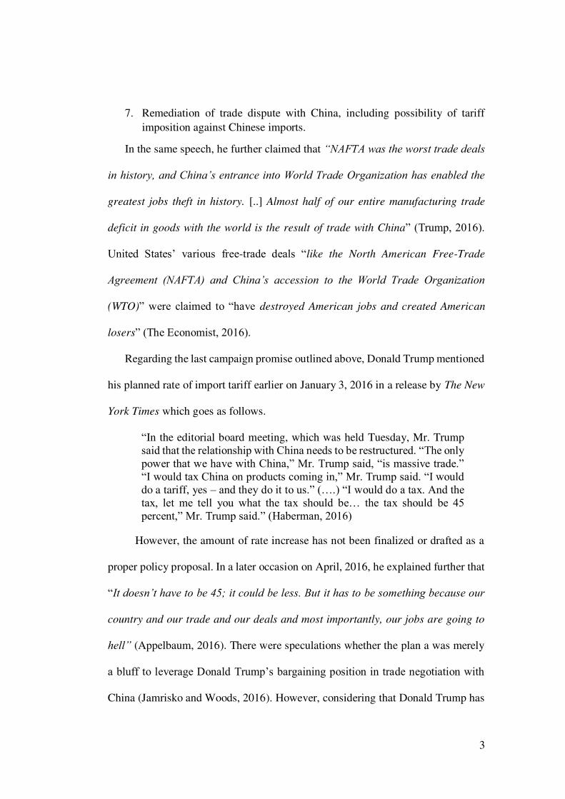
The extent of which two country’s import and export are compatible with

each other can be measured using trade complementarity index by Michaely (1997).

The index measures how much a country’s export structure matches its partner’s

import structure. According to the index (see Figure 3), United States import

structure have gotten more compatible with China’s export structure, making the

country pair a natural trading partner (WTO, 2012, 30-31). The compatibility was

also in line with increasing share of China in United States’ total trade volume.

However, rising complementarity between two countries was only one-sided.

According to the index, while China’s export has gotten more compatible with

United States’ import structure, the opposite occurred for United States’ export to

China. This situation had contributed to deteriorating United States’ trade balance

deficit with China.

Figure 3 about here.

Judging from high intensity and complementarity between United States and

China, it can be inferred a priory that any trade protectionism measures between

two countries will lead to large trade pattern change in both countries. Due to rising

domestic import price from China relative to other countries’, United States could

divert its trade away from China—its natural trading partner—towards other

countries, vice versa. This phenomenon was coined as “trade deflection” by Bown

and Crowley (2007). Mechanism for this effect can be modeled using Armington

import substitution which was used in this research.

6

3. Literature Review

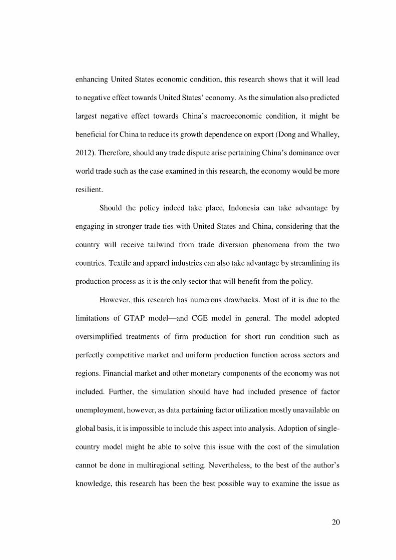
An import tariff puts a wedge between the world c.i.f. price and importing

country’s domestic consumer price. The policy is usually taken to protect domestic

producer from cheaper foreign goods. Rigorous partial equilibrium analysis has

been laid down by Krugman, et al. (2012: 192-202).

Assuming world price of a good (c.i.f. price, denoted as Pw) is lower than

domestic price, the economy will import D1 – S1 in quantity if there is no tariff

present (see Figure 4). An import tariff will raise the perceived consumer price to

Pt, decreasing its import demand. If the country’s import quantity is substantially

large in the world market, the decline in import demand will reduce global demand

of the good, thus, reducing the world price to Pt*. Hence, the resulting tariff will be

equivalent to Pt – Pt*. This will lead to less import quantity of D2 – S2.

Figure 4 around here.

The area of a, b, c, d, and e represents welfare change from imposition of

import tariff. Domestic consumer will suffer from decline of consumer surplus

equivalent to area a + b + c + d. Domestic producers’ surplus will increase by the

area of a. A tariff is a tax on imported goods, hence, the government will collect

tariff revenue equivalent to the size of tariff rate times import quantity represented

by the area of c + e. Triangle b and d is welfare loss due to imposition of a tariff.

Terms of trade will increase due to decline in country’s import commodity price

relative to export commodity price. Its gain is reflected under the area of e. Net

welfare effect is, therefore, will be ambiguous as it depends whether terms-of-trade

gain (area e) outweighs welfare loss (area c+e).

7

However, the above analysis rested on the assumption of perfectly

competitive market. In the presence of a single domestic monopolist firm, tariff

increase will have another distinctive aspect: it allows domestic monopolist to price

above its marginal cost and domestic consumption to decline while the monopolist

domestic marginal revenue increases. The monopolist will take advantage of the

difference between marginal cost and domestic price by selling the gap between its

production and domestic consumption to world market at world price, creating a

dumping policy (Rieber, 1981). Armington (1969) proposed a concept of elasticity

of substitution that will render similar goods coming from different sources as

imperfect substitutes. This relationship can be represented using constant elasticity

of substitution (CES) function.

The demand is determined by (1) total demand for good 𝑖 (𝑋𝑖 ), (2) ratio

between price of the good from 𝑗 source and its average price, (3) share of the good

from source 𝑗 (𝑏𝑖𝑗), and (4) elasticity of substitution in i-th market (𝜎𝑖). The larger

the value of 𝜎𝑖 , the more quantity demanded of i-th good from source 𝑗 will change

when there is a change in relative price of the good from j-th source. “Source” can

refer to either a country, country group, or domestic-foreign.

The CGE model used in this paper also incorporates Armington import

substitution mechanism written in CES functional form. Both between-countries

and between-foreign-and-domestic substitution nests are represented in this

mechanism (Hertel eds. 1997, 39-41). If an import tariff is levied, it will alter

domestic-foreign relative price and between-countries relative price. The change in

8

quantity demanded of a specific source will be governed by its relative price and its

degree of substitute.

An import tariff has been proven empirically to lead to decline in import

demand. USITC (2009) GTAP model simulation found that in the absence of tariff,

India’s trade with United States would have been around US$ 200-291 higher.

Elsheikh et al. (2015) study found out that a decrease in Sudan’s import tariff will

increase the country’s wheat imports. In multi-country setting, a trade restriction

measure will introduce a phenomenon called “trade deflection”—a decline of

export to tariff-enacting country accompanied by an increase of export to other third

country (Bown and Crowley, 2007). The deflection phenomenon was also

examined and confirmed by Dong and Whalley (2012) and Chandra (2017).

Aside from trade flow re-balancing, previous literature also examined

adverse effect of import tariff increase on various macroeconomic variables.

Chauvin and Ramos (2012) conducted a MIRAGE CGE model simulation of

common increase in tariff among MERCOSUR countries. The simulation predicted

mixed response in GDP and terms of trade. Mahadevan et al. (2017) dynamic CGE

model simulation of Indonesia’s rising mineral and general trade protectionism

projected negative impact to GDP, household consumption, and employment.

Noland et al. (2016) conducted a Moody’s DSGE model simulation of

United States economy in the presence of Donald Trump’s tariff increase policy on

Chinese and Mexican imports. The study found out that under the full trade war

scenario employment will fall more than 4 percent with largest job loss suffered by

non-trade services sector. The rising unemployment will cause drop in domestic

9

consumption and investment. Scenarios of aborted trade war in which China and

Mexico concede to United States demands shows softer repercussion to

consumption, unemployment rate, and GDP growth. However, the research did not

incorporate the policy in a multi-country setting, focusing only on domestic United

States macro-economy.

Prolonged United States-China bilateral trade balance deficit was already

predicted to spark tensions between both countries earlier in the study by Dong and

Whalley (2012). Their simulation study of bilateral United States-China tariff war

predicted shrinking world trade, welfare loss in both countries, and trade diversion.

They suggested trade re-balancing to alleviate China’s vulnerability from foreign

trade shocks.

In the case of country-specific tariff, there is a possibility for the impacted

country to “pass through” and re-brand its exports to another non-tariff impacted

countries. Gardner and Kimbrough’s model (Gardner and Kimbrough, 1990)

stipulated that a country-specific tariff will not have an impact on welfare allocation

but simply alters the world’s pattern of trade. However, the effect will not occur if

the tariff-imposing country adopts rules-of-origin to deter merchandise re-branding.

An import tariff is likely to be responded by retaliation from its partner

country. Scitovszky (1942) argued that by retaliating, a country can reclaim its

welfare loss generated by partner country’s import tariff. However, as the country

later recognizes that raising tariff will be responded by retaliation, both country will

come into agreement of a common tariff.

10

Post (1987) later extended analysis on country retaliation response by

assuming perfect foresight—each country expects that its trading partner will

always respond to changes in tariffs. The model developed various scenarios of

response ranging from symmetric retaliation to opposite direction response and

measured the welfare outcome from each option. Although a country could provide

a respond based on its subjective beliefs on welfare effects, the optimal solution

that provides highest welfare is by imposing similar tariff increase.

Does President Trump indeed have the authority to invoke the policy?

Huffbauer (2016) analyzed its feasibility from legal and political standpoint and

discovered that United States grants conditional authority to its president regarding

tariff increase measures. The conditions vary from requiring prior investigation of

industrial injury by US International Trade Commission, permission from Congress,

justification of unfair trade, to requiring declaration of national economic

emergency. Nevertheless, the policy is projected to face numerous objections both

from Congress and multinational firms.

The adverse effect brought by tariff increase will cause Trump to “face

vigorous court challenges by adversely affected US firms and possibly some states,

arguing that the president had exercised powers and invoked statutes in ways that

the Constitution or Congress never intended”. The court procedure, however,

“would be difficult and would certainly take time. Thus, at least for a few years, a

president Trump would have stronger legal hand and his actions would very likely

survive challenge in the US courts and Congress” (Huffbauer, 2016).

11

Based on the above literature, simulation scenarios in this research

incorporated tariff retaliation by China due to it being the country’s best response

for the policy. Retaliation is introduced by simulating similar level of United States’

tariff increase in China import tariff. Rule-of-origin is also assumed to be in place

to simplify the analysis. The model was adjusted to depict short-run condition due

to the possibility of court challenges faced by Donald Trump years after the policy

was in effect.

4. Methodology

4.1. Data

This study utilized Global Trade Analysis Project (GTAP) Database version 9A

from Center for Global Trade Analysis, Purdue University. The database covers

140 regional units and 57 sectors (Aguiar, et al. 2016) with reference year 2004,

2007, and 2011. The latest reference year was used in model calibration.

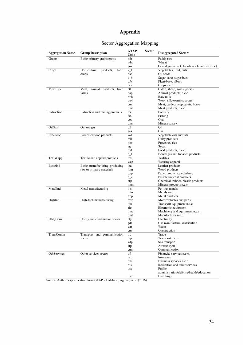
4.2. Aggregation

This research followed default GTAP database sector aggregation mapping with

further dis-aggregation of “GrainCrops”, “Extraction”, and manufacturing sector to

provide more detailed analysis (see Apendix for details). Countries were mapped

into 1-to-1 mapping for each of United States’ major trading partners making up 95

percent of its total trade volume in 2016. African countries were grouped into

“Africa”, 28 European Union countries were grouped as “EU-28”, and both

Australia and New Zealand were grouped as “Australia-Oceania”. Other countries

were mapped into “Rest-of-the-World” category (see see Apendix for details).

12

Factors of production were aggregated into “Land”, “Skilled Labor”,

“Unskilled Labor”, “Capital”, and “Natural Resources” category (see Apendix for

details). Land and natural resources were set to have limited mobility across sectors.

To achieve short-run simulation result, capital goods were also assumed to have

limited mobility (Burfisher, 2011, 137; Adams, 2005). The value of ETRAE for

capital goods is assumed to be similar with those of land.

4.3. Simulation

This study employs tariff policy simulation using Global Trade Analysis Project

(GTAP) CGE (Computable General Equilibrium) model (Hertel, eds. 1997). The

model can calculate likely outcomes of the tariff policy ex-ante via mathematical

simulation. Simulation study is suitable for this research as there are currently no

ex-post data generated from the policy.

As both China and United States are large economies, their trade policy

could send repercussions to other countries. A CGE model can capture these

linkages through price mechanism (Hosoe, et al., 2010, 2-3). The simulation is of

general equilibrium in nature, meaning that it also captures both direct and indirect

effect stemming from linkages across different countries and markets. Moreover,

GTAP model was specifically chosen due to its extensive treatments of inter-

regional trade which is deemed to be suitable for conducting global trade policy

analysis.

4.4. The GTAP Model

GTAP model is a CGE model developed by Center for Global Trade Analysis,

Purdue University. The full model was introduced in Hertel (ed., 1997). Aside from

extensive modeling of inter-regional linkages—mainly via international trade—it

13

also models demand for domestic and foreign-produced goods, international

transport cost, global investment allocation, regional household demand, and

welfare decomposition (Hertel, 2013). The model uses GTAP database for

calibration.

GTAP model followed MONASH-style approach in CGE modeling (Dixon

and Jorgenson, 2013, 23). Most of its behavioral and identity equations were

represented in percentage-change form rather than in level-form. The model will

not solve for maximization or minimization problem as with several other CGE

models, however, the problem was already implicitly specified within its equations.

The model’s mathematical functions were derived from constrained optimization

problem.

In brief, the model has the following properties (Hertel, ed., 1997; GTAP

Version 6.2 TABLO Code, 2003).

1. It models the behavior of firms and three regional households (private

household, government household, and savings expenditure) in each

region 𝑟.

2. Firms minimize their cost of production subject to production

technology represented in Constant Elasticity of Substitution (CES)

functional form. Firms are assumed to be price takers.

3. Regional households maximize their utility subject to income from net

payments of factor use (for private household) or revenue of government

distortionary measures (for government household). Regional

household utility is the sum of its three sub-components per capita under

14

the assumption of separate utility from consumption of public and

private goods (Hertel, 2013, 827).

4. Private household expenditure are modeled using Constant Difference

Elasticity functional form by Hanoch (1975) to account for its non-

homothetic preferences.

5. “Margin commodity” is introduced as a proxy for transportation cost.

6. Savings from regional household are spent on global investment

portfolio, with special treatment regarding lack of intertemporal closure

in the model.

7. Imports are differentiated by source and governed by Armington import

substitution elasticity parameter.

4.5. Computation

For computation, both GTAP database and GTAP model use GEMPACK (General

Equilibrium Modeling Package) software (Harrison and Pearson, 1996) developed

by Center of Policy Studies, Victoria University, Melbourne, Australia. In this

research, runGTAP software—a GEMPACK interface for GTAP model

simulation—was used to perform model simulations. This research employed

standard version of GTAP Model version 6.2 (Global Trade Analysis Project, 2003),

the latest version after several revisions regarding various modeling issues (Itakura

and Hertel, 2001).

This research used Gragg’s 4-6-8 steps solution method with “automatic

accuracy” option enabled to provide maximum result accuracy (Horridge, 2001).

The method divides the shock with interpolation into small increments and iterates

15

the calculation several times. The final and accurate solution are obtained from

average value of each iteration’s solutions.

4.6. Scenarios

Donald Trump’s proposed tariff increased policy was simulated under the following

scenarios.

1. Full trade protection scenario: United States imposes 45 percent import

tariff on all commodities obtained from China. China retaliates by imposing

similar percentage point of tariff increase.

2. Manufacturing trade protection scenario: United States imposes 45 percent

import tariff only on manufacturing commodities (“ProcFood”,

“TextWapp”,”BasicInd”, “MetalInd”, and “HighInd”). China retaliates by

imposing similar tariff rate increase on manufacturing import from United

States.

GTAP model’s “standard general equilibrium closure” was adopted for all

simulations. Under this closure, price elasticity parameters can respond to shock

from both supply and demand side (Hertel, ed, 1997, 158-159).

5. Results and Discussions

5.1. Impacts of Global Economy

GTAP Model predicted negative impact to China and United States’ GDP (see

Table 1). Although both scenarios simulated symmetric tariff increase in both

United States and China, impact on China’s GDP is larger than those of United

States’. Manufacturing-only protection scenario generally predicted milder impact

to GDP compared to full protection scenario. The impact on another countries’ GDP

16

varies from strongly positive (for Vietnam, Mexico, and Canada) to slightly above

zero. The projection of decline in both tariff imposing countries’ GDP is in line

with prior studies in the case of US (Noland, et al., 2016) and Indonesia

(Mahadevan, et al., 2017) while contradicts Chauvin and Ramos (2012) study of

MERCOSUR tariff escalation case.

Table 1 about here.

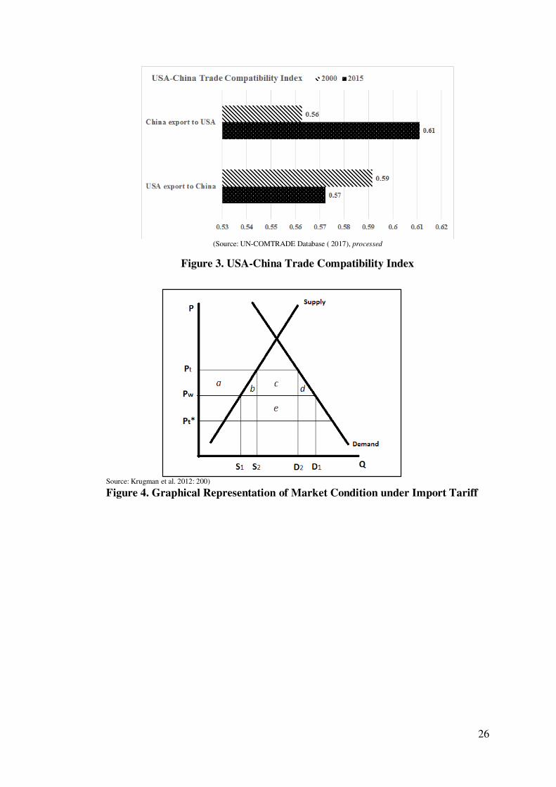
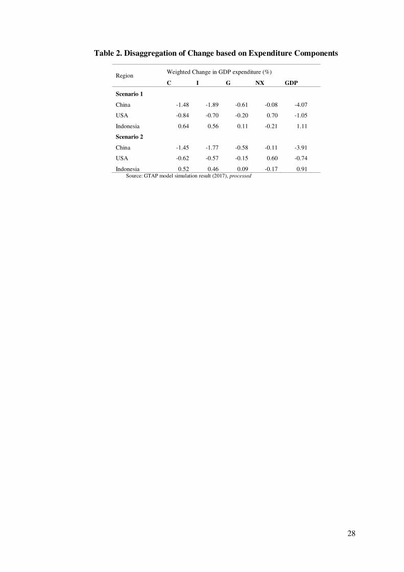
Disaggregating the percentage change according to its expenditure

components gives a better picture of the change. In China, consumption, investment,

and government expenditures were projected to decline sharply in both scenarios

while net export experiences a rise. In the United States, net export was projected

to decline with subdued decline in investment, consumption and government

expenditure. (see Table 2). Indonesia was projected to experience mild increase in

GDP around 0.91 percent to 1.11 percent under first and second scenario,

respectively. The change is contributed by increase in investment and consumption

expenditure component.

Table 2 about here.

Table 3 reports predicted change in trade balance (in million USD) due to

the policy. United States trade balance will experience sharp positive change while

China’s change trade balance is comparable with those of other countries’. EU-28

countries, albeit reported to experience largest change, comprises of smaller

changes within its country members comparable to those of other countries in the

list. Japan and Brazil is the only country that will suffer from relatively large decline

in trade balance compared to other countries.

17

Table 3 about here.

Equivalent variation is used by GTAP model as a measurement of a

country’s welfare gain or loss. Table 4 reports welfare gain or loss for each country.

Only China and United States will suffer from welfare loss due to the tariff increase.

This result contradicts simulation results by Dong and Whalley (2012) both in their

Armington model and endogenous trade surplus model results.

Table 4 about here.

Predicted impact to change in terms-of-trade shows similar pattern to those

of change in GDP (see table 5). Only China and United States will suffer from sharp

worsening of terms of trade. China was predicted to experience the largest decline.

Other countries will experience change in terms of trade around zero with Turkey

being the only country to experience negative change. World price was not

projected to change significantly, indicating that the tariff war will not yield

significantly large world trade volume change.

The simulation result shows that the change in terms of trade is mainly

contributed by change in export price. The phenomenon is more pronounced in

China and United States where predicted negative change in both country’s export

price is very sharp. This is due to decline in both country’s general decline in

demand, bringing their f.o.b. export price lower.

There is also a possibility of deflection towards domestically produced

goods as asserted by Burfisher (2011, 157). She argued that since imported goods

will be more expensive under import tariff, both countries will shift their demand

towards domestic goods, bringing down their export supply and increasing their

18

export price. However, the domestic diversion phenomenon is overshadowed by

overall increase in both China’s and United States’ export towards each of their

other trading partners.

Table 5 about here.

The export diversion effect towards other trading partner (Bown and

Crowley, 2007; Chandra, 2017) is evident in both scenarios (see Table 6). As GTAP

model only calculates price change and quantity change for region-specific trade,

these percentage change in export value is obtained by using multiplication rule of

price change and quantity change. Bilateral trade between China and United States

is predicted to experience sharp decline, similar to US-China tariff war simulation

by Dong and Whalley (2012) despite differences in the effect towards other trading

partner countries. The diversion is larger in China than United States and in line

with prediction of larger decline in China’s export price.

Table 6 about here.

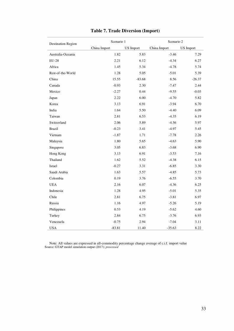
Literature of trade diversion only mentioned change in export pattern.

However, looking at change in import pattern can show the impact on other

countries’ export towards China and United States. Table 7 presents change in

import pattern. A riveting result is that, under manufacturing-only protection

scenario, China import will diminish. This result is contrast with first scenario

where import diversion was predicted by the model. Disaggregating the effect based

on the commodity, simulation result shows that import diversion for primary

commodities which were present under scenario 1 is absent in scenario 2. The

policy under scenario 2 is levied on China’s surplus commodities, therefore, China

19

will not substitute such commodities towards other trading partners. Instead of

deflecting its import, general decline in import demand as result of general output

contraction is more pronounced in the projection.

Table 7 about here.

6. Concluding Remarks

This research examined the possible impacts of Donald Trump’s proposed import

tariff increase towards Chinese imports on global economy using GTAP standard

model. The simulation scenarios depicted short-run effects of full-protection and

manufacturing protection with appropriate retaliation response from China. On

global level, the policy was projected to lead to decline in GDP, terms-of-trade, and

welfare; and increase in trade balance for United States and China. The results

confirmed previous news pundits’ predictions of declining GDP and negative

welfare effect; and was mostly in line with previous trade simulation studies

involving tariff increase policy. Other country will experience mixed impact on

their macroeconomic variables.

Trade diversion phenomena was present in the simulation results, predicting

steep decline in bilateral trade between the two countries and increasing export

towards their third trading partners. Import pattern of both countries will also

change as well, although under second scenario, China’s import from all countries

will generally decline. In general, second scenario simulation results show milder

impact of the policy on all observed variables.

Simulation results shows that the goal of “Reclaiming American Economic

Independence” will not be attained by imposing strict import tariff. Instead of

20

enhancing United States economic condition, this research shows that it will lead

to negative effect towards United States’ economy. As the simulation also predicted

largest negative effect towards China’s macroeconomic condition, it might be

beneficial for China to reduce its growth dependence on export (Dong and Whalley,

2012). Therefore, should any trade dispute arise pertaining China’s dominance over

world trade such as the case examined in this research, the economy would be more

resilient.

Should the policy indeed take place, Indonesia can take advantage by

engaging in stronger trade ties with United States and China, considering that the

country will receive tailwind from trade diversion phenomena from the two

countries. Textile and apparel industries can also take advantage by streamlining its

production process as it is the only sector that will benefit from the policy.

However, this research has numerous drawbacks. Most of it is due to the

limitations of GTAP model—and CGE model in general. The model adopted

oversimplified treatments of firm production for short run condition such as

perfectly competitive market and uniform production function across sectors and

regions. Financial market and other monetary components of the economy was not

included. Further, the simulation should have had included presence of factor

unemployment, however, as data pertaining factor utilization mostly unavailable on

global basis, it is impossible to include this aspect into analysis. Adoption of single-

country model might be able to solve this issue with the cost of the simulation

cannot be done in multiregional setting. Nevertheless, to the best of the author’s

knowledge, this research has been the best possible way to examine the issue as

21

there are almost no other multiregional trade models available to serve for the

analysis.

References

Adams, Philip D. 2005. “Interpretation of Results from CGE Models such as GTAP.” Journal of Policy Modeling 27 (8): 941–59.

doi:10.1016/j.jpolmod.2005.06.002.

Aguiar, Angel, Badri Narayanan, and Robert McDougall. 2016. “An Overview of the GTAP 9 Data Base.” Journal of Global Economic Analysis 1 (1): 181–208. doi:10.21642/JGEA.010103AF.

Appelbaum, Binyamin. 2016. “Experts Warn of Backlash in Donald Trump’s China Trade Policies.” The New York Times.

https://www.nytimes.com/2016/05/03/us/politics/donald?trump?trade?policy

?china.html?_r=0.

Armington, Paul S. 1969. “A Theory of Demand for Products Distinguished by Place of Production.” IMF Staff Papers 16 (1): 159–78.

doi:10.2307/3866403.

Bown, Chad P., and Meredith A. Crowley. 2007. “Trade Deflection and Trade Depression.” Journal of International Economics 71 (3): 176–201.

doi:10.1016/j.jinteco.2006.09.005.

Bryan, Bob. 2016. “Trump’s New Tariff Proposal Could Put the Economy on a

Path to ‘Global Recession.’” Business Insider.

http://www.businessinsider.co.id/trump-trade-policy-lead-to-global-

recession-2016-12/?r=US&IR=T#v8mFpklgSx4zbgpV.97.

Burfisher, Mary E. 2011. Introduction to Computable General Equilibrium

Models. Cambridge: Cambridge University Press.

Chandra, Piyush. 2016. “Impact of Temporary Trade Barriers: Evidence from China.” China Economic Review 38. Elsevier Inc.: 24–48.

doi:10.1016/j.chieco.2015.11.002.

Dixon, Peter B., and Dale W. Jorgenson. 2013. “Introduction.” Handbook of

Computable General Equilibrium Modeling 1: 1–103.

22

Dong, Yan, and John Whalley. 2012. “Gains and Losses from Potential Bilateral US-China Trade Retaliation.” Economic Modelling 29 (6). Elsevier B.V.:

2226–36. doi:10.1016/j.econmod.2012.07.001.

Elliott, Larry. 2016. “How America’s New President Will Affect the Global Economy.” The Guardian.

https://www.theguardian.com/business/2016/nov/09/donald-trump-new-us-

president-america-global-economy-china-mexico.

Elsheikh, Omer Elgaili, Azharia Abdelbagi Elbushra, and Ali A.A. Salih. 2015.

“Economic Impacts of Changes in Wheat’s Import Tariff on the Sudanese Economy.” Journal of the Saudi Society of Agricultural Sciences 14 (1).

King Saud University and Saudi Society of Agricultural Sciences: 68–75.

doi:10.1016/j.jssas.2013.08.002.

Gardner, Grant W, and Kent P Kimbrough. 1990. “The Economics of Country-

Specific Tariffs.” International Economic Review 31 (3): 575–88.

http://www.jstor.org/stable/2527162.

Global Trade Analysis Project. 2003. “GTAP TABLO Code Version 6.2.” West Lafayette: Center for Global Trade Analysis Purdue University.

Gohin, Alexandre, and Thomas W. Hertel. 2001. “A Note on the CES Functional Form and Its Use in the GTAP Model.” GTAP Research Memorandum, no.

2. https://www.gtap.agecon.purdue.edu/resources/download/1610.pdf.

Haberman, Maggie. 2016. “Donald Trump Says He Favors Big Tariffs on Chinese Exports.” The New York Times. http://www.nytimes.com/politics/first-

draft/2016/01/07/donald-trump-says-he-favors-big-tariffs-on-chinese-

exports/.

Hanoch, Giora. 1975. “Production and Demand Models with Direct or Indirect Implicit Additivity.” Econometrica 43 (3): 395–419.

http://www.jstor.org/stable/1914273.

Harrison, W. Jill, and K. R. Pearson. 1996. “Computing Solutions for Large General Equilibrium Models Using GEMPACK.” Computational Economics

9: 83–127. doi:10.1007/BF00123638.

Hertel, Thomas W., ed. 1997. Global Trade Analysis: Modeling and Application.

Cambridge: Cambridge University Press.

Hertel, Thomas W. 2013. “Global Applied General Equilibrium Analysis Using

the GTAP Framework.” Handbook of Computable General Equilibrium

Modeling 1: 815–76.

23

Horridge, Mark. 2001. “MINIMAL: A Simplified General Equilibrium Model.” Centre of Policy Studies and the Impact Project. Clayton: Monash

University.

Hosoe, Nobuhiro, Kenji Gasawa, and Hideo Hashimoto. 2010. Textbook of

Computable General Equilibrium Modelling: Programming and Simulations.

London: Palgrave Macmillan.

Hufbauer, Gary Clyde. 2016. “Could a President Trump Shackle Imports?” In Assessing Trade Agendas in the US Presidential Campaign, 5–16.

Washington DC: Peterson Institute of International Economics.

https://piie.com/sites/default/files/supporters.pdf.

Itakura, Ken, and Thomas W. Hertel. 2001. “A Note On Changes Since GTAP Book Model (Version 2.2a/GTAP94).” GTAP Resource #721.

https://www.gtap.agecon.purdue.edu/resources/res_display.asp?RecordID=7

21.

Jamrisko, Michelle, and Randy Woods. 2016. “Trump Talk of Higher Tariffs a Bargaining Chip, Scaramucci Says.” Bloomberg.

https://www.bloomberg.com/news/articles/2016?12?01/trump?talk?of?higher

Krugman, Paul R., Maurice Obstfeld, and Marc Melitz. 2012. International

Economics: Theory and Policy. Boston: Pearson Addison-Wesley.

Mahadevan, Renuka, Anda Nugroho, and Hidayat Amir. 2017. “Do Inward Looking Trade Policies Affect Poverty and Income Inequality? Evidence

from Indonesia’s Recent Wave of Rising Protectionism.” Economic

Modelling 62 (January). Elsevier: 23–34.

doi:10.1016/j.econmod.2016.12.031.

Martin, Eric. 2017. “Why Trump’s ‘Big Border Tax’ Gets Taken Seriously: QuickTake Q&A.” Bloomberg.

https://www.bloomberg.com/politics/articles/2017?01?18/why?trump?s?tarif

f?threats?get?taken?so?seriously?quicktake?q?a.

McDougall, Robert. 2003. “A New Regional Household Demand System for GTAP.” GTAP Technical Paper No. 20 2 (20): 1–61.

Michaely, Michael. 1996. “Trade Preferential Agreements in Latin America: An Ex-Ante Assessment.” World Bank Policy Research Working Paper 1583.

Washington DC.

Nicolas, Depetris Chauvin, and Ramos Priscila. 2012. The Welfare Impact of

Protectionism in Latin America: Evaluation of Alternative Scenarios.

24

ANALES Asociacion Argentina de Economia Politica XLVII Reunión Anual.

http://www.aaep.org.ar/anales/works/works2012/Depetris.pdf.

Noland, Marcus, Sherman Robinson, and Tyler Moran. 2016. “Impact of Clinton’s and Trump’s Trade Proposals.” In Assessing Trade Agendas in the

US Presidential Campaign. Washington DC: Peterson Institute of

International Economics.

Post, Gerald V. 1987. “Optimal Tariffs and Retaliation with Perfect Foresight.” Journal of International Economic Integration 2 (1): 54–70.

http://www.jstor.org/stable/23000112.

Rieber, By William J. 1981. “Tariffs as a Means of Altering Trade Patterns.” The

American Economic Review 71 (5): 1098–99.

http://www.jstor.org/stable/1803498.

Scitovszky, T De. 1942. “A Reconsideration of the Theory of Tariffs.” The

Review of Economic Studies 9 (2): 89–110.

doi:10.1126/science.151.3712.867-a.

The Economist. 2017. “Dealing with Donald: Donald Trump’s Trade Bluster.” The Economist. http://www.economist.com/news/briefing/21711498-

whatever-he-thinks-...

Trump, Donald. 2016. “Declaring American Economic Independence.” Donald J.

Trump For President.

https://assets.donaldjtrump.com/DJT_DeclaringAmericanEconomicIndepend

ence.pdf.

USITC. 2009. “India : Effects of Tariffs and Nontariff Measures on U.S. Agricultural Exports.” Washington DC. http://www.usitc.gov/publications/332/pub4107.pdf.

WTO. 2012. A Practical Guide to Trade Policy Analysis. Geneva: World Trade

Organization.

25

Source: World Bank WITS Database (2017), processed

Figure 1. United States Top 5 Trading Partner Countries' Share in Total Trade

Sounce: World Bank WITS Database, (2017), processed

Figure 2. China's Top 5 Trading Partner Country's Share in Total Trade

26

(Source: UN-COMTRADE Database ( 2017), processed

Figure 3. USA-China Trade Compatibility Index

Source: Krugman et al. 2012: 200)

Figure 4. Graphical Representation of Market Condition under Import Tariff

27

Table 1. Impact on GDP

Region Change in GDP (%)

Scenario 1 Scenario 2

Australia-Oceania 0.89 0.52

EU-28 0.7 0.63

Africa 0.87 0.73

Rest-of-the-World 1 0.86

China -4.1 -3.93

Canada 2.43 2.29

Mexico 3.24 3.19

Japan 1 0.97

Korea 0.9 0.87

India 0.87 0.67

Taiwan 0.81 0.79

Switzerland 0.71 0.63

Brazil 1.57 0.98

Vietnam 3.66 3.42

Malaysia 1.17 1.1

Singapore 0.62 0.54

Hong Kong 0.58 0.33

Thailand 1.04 0.89

Israel 2 1.93

Saudi Arabia 0.87 0.79

Colombia 1.55 1.42

UEA 0.77 0.67

Indonesia 1.01 0.87

Chile 0.74 0.61

Russia 1 0.9

Philippines 1.42 1.29

Turkey 0.44 0.32

Venezuela 1.42 1.32

USA -0.92 -0.66 Source: GTAP model simulation result (2017), processed.

28

Table 2. Disaggregation of Change based on Expenditure Components

Region Weighted Change in GDP expenditure (%)

C I G NX GDP

Scenario 1

China -1.48 -1.89 -0.61 -0.08 -4.07

USA -0.84 -0.70 -0.20 0.70 -1.05

Indonesia 0.64 0.56 0.11 -0.21 1.11

Scenario 2

China -1.45 -1.77 -0.58 -0.11 -3.91

USA -0.62 -0.57 -0.15 0.60 -0.74

Indonesia 0.52 0.46 0.09 -0.17 0.91 Source: GTAP model simulation result (2017), processed

29

Table 3. Change in Trade Balance

Change in Trade Balance

Region Scenario 1 Scenario 2

Australia-Oceania -3656.16 -2141.6

EU-28 -33671.11 -27954.12

Africa -2230.44 -1934.7

Rest-of-the-World -8477.04 -7482.46

China -6129.2 -8382.2

Canada -5390.34 -4709.72

Mexico -2907.57 -2645.16

Japan -15385.15 -14024.9

Korea -3026.27 -2745.15

India -3477.06 -2741.36

Taiwan -347.49 -291.45

Switzerland -824.81 -664.99

Brazil -7696.42 -4017.27

Vietnam -2788.98 -2614.29

Malaysia -1294.45 -1200.49

Singapore 149.55 104.71

Hong Kong -461.01 -349.5

Thailand -1197.26 -1109.45

Israel -1178.93 -1059.72

Saudi Arabia 997.96 1008.25

Colombia -800.42 -717.34

UEA -804.95 -717.21

Indonesia -1743.13 -1407.05

Chile -300.24 -220.83

Russia -3172.77 -2744.74

Philippines -1036.56 -913.78

Turkey -1051.08 -805.22

Venezuela -302.91 -261.02

USA 108203.75 92742.91 Source: GTAP model simulation result (2017), processed.

30

Table 4. Equivalent Variation

Region Scenario 1 Scenario 2

Australia-Oceania 2078.51 476.1

EU-28 14419.18 13130.71

Africa 4665.28 4320.04

Rest-of-the-World 15232.55 14119.64

China -100994.8 -94061.28

Canada 8739.55 7709.65

Mexico 7887.86 7626.97

Japan 7038.48 7015.53

Korea 2591.64 2521.56

India 2108.03 1454.4

Taiwan 964.4 913.82

Switzerland 428.18 367.49

Brazil 4288.02 1962.76

Vietnam 2584.54 2452.52

Malaysia 1543.79 1487.98

Singapore 340.4 256.75

Hong Kong 786.1 493.54

Thailand 1028.02 856.2

Israel 1321.64 1279.76

Saudi Arabia 2426.23 2444.18

Colombia 604.85 572.67

UEA 1724.22 1673.53

Indonesia 1370.57 983.21

Chile 254.97 116.61

Russia 5370.94 5292.72

Philippines 668.61 612.38

Turkey 31.51 -214.57

Venezuela 879.08 857.59

USA -90881.03 -79528.23 Source: GTAP model simulation result (2017), processed.

31

Table 5. Terms of Trade Change

Region

Scenario 1 Scenario 2

World Price

Contrib.

Export price

contrib.

Import price

contrib

Terms-of-

trade

World Price

Contrib.

Export price

contrib.

Import price

contrib

Terms-of-

trade

Australia-Oceania 0.05 0.25 -0.22 0.52 -0.06 -0.02 -0.22 0.13

EU-28 -0.06 0.28 0.05 0.16 -0.06 0.25 0.05 0.14

Africa 0.43 0.22 -0.16 0.81 0.42 0.16 -0.17 0.75

Rest-of-the-

World 0.34 0.33 -0.07 0.74 0.33 0.28 -0.08 0.69

China -0.23 -2.55 0.26 -3.03 -0.22 -2.51 0.22 -2.94

Canada 0.13 1.16 -0.26 1.56 0.13 1.14 -0.11 1.39

Mexico 0.02 1.8 -0.33 2.16 0.03 1.87 -0.17 2.08

Japan -0.25 0.51 -0.42 0.69 -0.22 0.51 -0.4 0.69

Korea -0.25 0.28 -0.3 0.33 -0.22 0.28 -0.28 0.34

India -0.29 0.42 -0.19 0.32 -0.29 0.31 -0.18 0.21

Taiwan -0.21 0.34 -0.17 0.3 -0.2 0.35 -0.13 0.29

Switzerland 0.01 0.31 0.18 0.14 0.01 0.28 0.16 0.13

Brazil 0.02 0.85 -0.15 1.02 -0.02 0.25 -0.13 0.36

Vietnam 0.02 1.14 -0.44 1.6 0.01 1.04 -0.44 1.49

Malaysia 0.07 0.38 -0.17 0.62 0.06 0.37 -0.18 0.61

Singapore -0.13 0.15 -0.08 0.11 -0.13 0.13 -0.08 0.08

Hong Kong 0.05 0.08 -0.32 0.44 0.03 -0.05 -0.3 0.29

Thailand -0.13 0.37 -0.13 0.37 -0.14 0.31 -0.13 0.3

Israel -0.08 1.05 -0.05 1.02 -0.07 1.04 -0.02 0.99

Saudi Arabia 0.83 0.1 -0.09 1.01 0.84 0.09 -0.08 1.01

Colombia 0.39 0.39 -0.03 0.8 0.36 0.43 0.01 0.78

UEA 0.63 0.11 -0.14 0.88 0.63 0.09 -0.15 0.87

Indonesia 0.09 0.4 -0.2 0.68 0.01 0.32 -0.19 0.52

Chile -0.04 0.13 -0.2 0.29 -0.09 0.06 -0.17 0.15

Russia 0.62 0.25 -0.11 0.98 0.61 0.24 -0.12 0.98

Philippines -0.14 0.59 -0.23 0.67 -0.13 0.52 -0.23 0.62

Turkey -0.19 0.2 0 0.02 -0.21 0.16 0.03 -0.07

Venezuela 0.74 0.36 -0.09 1.19 0.74 0.34 -0.09 1.17

USA -0.09 -0.66 0.32 -1.06 -0.08 -0.31 0.29 -0.68 Source: GTAP model simulation output (2017), processed.

32

Table 6. Trade Diversion (Export)

Destination Region Scenario 1 Scenario 2

China Export US Export China Export US Export

Australia-Oceania 11.72 4.14 11.33 0.55

EU-28 12.52 5.37 12.86 2.03

Africa 12.33 4.85 12.55 1.59

Rest-of-the-World 12.59 5.10 12.87 2.02

China 15.55 -83.94 8.56 -35.66

Canada 12.15 4.04 13.83 2.83

Mexico 13.47 5.20 15.54 4.16

Japan 10.35 2.92 11.13 0.62

Korea 10.23 2.77 11.03 0.46

India 12.22 4.82 12.25 1.39

Taiwan 10.95 3.02 12.14 1.16

Switzerland 13.17 5.82 13.48 2.45

Brazil 13.36 5.91 12.81 1.94

Vietnam 13.39 5.84 13.52 2.65

Malaysia 11.76 4.27 11.81 1.17

Singapore 11.82 4.03 12.00 1.14

Hong Kong 10.58 2.88 11.13 0.28

Thailand 12.05 4.27 12.16 1.21

Israel 13.16 5.48 13.90 2.86

Saudi Arabia 12.87 5.22 13.14 2.18

Colombia 13.21 5.24 14.13 2.89

UEA 12.11 4.52 12.38 1.48

Indonesia 12.32 4.76 12.45 1.77

Chile 11.30 4.06 11.67 0.93

Russia 12.81 5.24 13.00 2.06

Philippines 12.49 4.97 12.53 1.76

Turkey 12.01 4.30 12.75 1.68

Venezuela 14.22 6.34 14.58 3.26

USA -83.78 11.40 -26.49 8.22

Note: All values are expressed in all-commodity percentage change average of f.o.b. export value Source: GTAP model simulation output (2017); processed

33

Table 7. Trade Diversion (Import)

Destination Region Scenario 1 Scenario 2

China Import US Import China Import US Import

Australia-Oceania 1.82 5.83 -3.46 7.29

EU-28 2.21 6.12 -4.34 6.27

Africa 1.45 5.34 -4.78 5.74

Rest-of-the-World 1.28 5.05 -5.01 5.39

China 15.55 -83.68 8.56 -26.37

Canada -0.93 2.30 -7.47 2.44

Mexico -2.27 0.44 -9.55 -0.03

Japan 2.22 6.00 -4.70 5.82

Korea 3.13 6.91 -3.94 6.70

India 1.64 5.50 -4.40 6.09

Taiwan 2.81 6.53 -4.35 6.19

Switzerland 2.06 5.89 -4.56 5.97

Brazil -0.23 3.41 -4.97 5.45

Vietnam -1.87 1.71 -7.78 2.26

Malaysia 1.80 5.65 -4.63 5.90

Singapore 3.05 6.83 -3.68 6.90

Hong Kong 3.13 6.91 -3.53 7.16

Thailand 1.62 5.52 -4.38 6.15

Israel -0.27 3.31 -6.85 3.30

Saudi Arabia 1.63 5.57 -4.85 5.73

Colombia 0.19 3.76 -6.55 3.70

UEA 2.16 6.07 -4.36 6.25

Indonesia 1.28 4.95 -5.01 5.35

Chile 2.81 6.75 -3.81 6.97

Russia 1.16 4.97 -5.26 5.19

Philippines 0.53 4.19 -5.62 4.60

Turkey 2.84 6.75 -3.76 6.93

Venezuela -0.75 2.94 -7.04 3.11

USA -83.81 11.40 -35.63 8.22

Note: All values are expressed in all-commodity percentage change average of c.i.f. import value Source: GTAP model simulation output (2017); processed

34

Appendix

Sector Aggregation Mapping

Aggregation Name Group Description GTAP Sector Code

Disaggregated Sectors

Grains Basic primary grains crops pdr Paddy rice wht Wheat

gro Cereal grains, not elsewhere classified (n.e.c)

Crops Horticulture products, farm

crops

v_f Vegetables, fruit, nuts

osd Oil seeds

c_b Sugar cane, sugar beet pfb Plant-based fibers

ocr Crops n.e.c

MeatLstk Meat, animal products from

farms

ctl Cattle, sheep, goats, gorses

oap Animal products, n.e.c

rmk Raw milk wol Wool, silk-worm cocoons

cmt Meat, cattle, sheep, goats, horse

omt Meat products, n.e.c.

Extraction Extraction and mining products frs Forestry

fsh Fishing coa Coal

omn Minerals, n.e.c

OilGas Oil and gas oil Oil

gas Gas

ProcFood Processed food products vol Vegetable oils and fats

mil Dairy products

pcr Processed rice sgr Sugar

ofd Food products, n.e.c.

b_t Beverages and tobacco products

TextWapp Textile and apparel products tex Textiles

wap Wearing apparel

BasicInd Basic manufacturing producing

raw or primary materials

lea Leather products

lum Wood products ppp Paper products, publishing

p_c Petroleum, coal products

crp Chemical, rubber, plastic products nmm Mineral products n.e.c.

MetalInd Metal manufacturing i_s Ferrous metals nfm Metals n.e.c.

fmp Metal products

HighInd High-tech manufacturing mvh Motor vehicles and parts

otn Transport equipment n.e.c.

ele Electronic equipment ome Machinery and equipment n.e.c.

omf Manufactures n.e.c.

Util_Cons Utility and construction sector ely Electricity

gdt Gas manufacture, distribution

wtr Water cns Construction

TransComm Transport and communication sector

trd Trade otp Transport n.e.c.

wtp Sea transport

atp Air transport cmn Communication

OthServices Other services sector ofi Financial services n.e.c. isr Insurance

obs Business services n.e.c.

ros Recreation and other services osg Public

administration/defense/health/education dwe Dwellings

Source: Author’s specification from GTAP 9 Database; Aguiar, et al. (2016)

35

Regional Aggregation Mapping

Regions Members

AusOce Australia, New Zealand, Other Oceania

EU_28 Austria, Belgium, Cyprus, Czech Republic, Denmark, Estonia, Finland, Germany, Greece, Hungary,

Ireland, Italy, Latvia, Lithuania, Luxembourg, Malta, Netherlands, Poland, Portugal, Slovakia, Slovenia,

Spain, Sweden, United Kingdom, Bulgaria, Croatia, Romania

Africa Benin, Burkina Faso, Cameroon, Cote d’Ivoire, Ghana, Guinea, Nigeria, Senegal, Togo, Rest-of-Western

Africa, Central Africa, South Central Africa, Ethiopia, Kenya, Madagascar, Malawi, Mauritius, Mozambique, Rwanda, Tanzania, Uganda, Zambia, Zimbabwe, Rest of Eastern Africa, Botswana,

Namibia, South Africa, Rest of South African Countries.

China China

Canada Canada

Mexico Mexico Japan Japan

Korea Korea

India India Taiwan Taiwan

Switzerland Switzerland

Brazil Brazil Vietnam Vietnam

Malaysia Malaysia

Singapore Singapore Hongkong Hong Kong

Thailand Thailand

Israel Israel SaudiArb Saudi Arabia

Colombia Colombia

UEA UEA Indonesia Indonesia

Chile Chile

Russia Russia Phlpns Philippines

Turkey Turkey

Venzuela Venezuela USA USA

ROW Other countries not specified above

Source: Author’s specification from GTAP 9 Database

Factors of Production Aggregation Mapping

Factor of Production Aggregation Group Factor Mobility

Land “Land” Sluggish

(𝐸𝑇𝑅𝐴𝐸 = −1)

Technicians, Associates,

Professionals Skilled Labor

“SkLabor” Mobile

Officials and Managers,

Agricultural and Unskilled Unskilled Labor

“UnSkLabor” Mobile Clerks

Service / Shop workers

Capital “Capital” Sluggish (𝐸𝑇𝑅𝐴𝐸 = −1)

Natural Resources Natural Resources

“NatRes”

Sluggish (𝐸𝑇𝑅𝐴𝐸 = −0.001)

Source: Author’s specification from GTAP 9 Database