munich personal repec archive - uni- · pdf file0 3 5 $ munich personal repec archive stock...

MPRAMunich Personal RePEc Archive

Stock returns predictability and theadaptive market hypothesis in emergingmarkets: evidence from India

Gourishankar S Hiremath and Jyoti Kumari

Indian Institute of Technology Kharagpur

2014

Online at http://mpra.ub.uni-muenchen.de/58378/MPRA Paper No. 58378, posted 9. September 2014 20:13 UTC

http://mpra.ub.uni-muenchen.de/

http://mpra.ub.uni-muenchen.de/58378/

RESEARCH Open Access

Stock returns predictability and the adaptivemarket hypothesis in emerging markets: evidencefrom IndiaGourishankar S Hiremath* and Jyoti Kumari

Abstract

This study addresses the question of whether the adaptive market hypothesis provides a better description of thebehaviour of emerging stock market like India. We employed linear and nonlinear methods to evaluate thehypothesis empirically. The linear tests show a cyclical pattern in linear dependence suggesting that the Indianstock market switched between periods of efficiency and inefficiency. In contrast, the results from nonlinear testsreveal a strong evidence of nonlinearity in returns throughout the sample period with a sign of tapering magnitudeof nonlinear dependence in the recent period. The findings suggest that Indian stock market is moving towardsefficiency. The results provide additional insights on association between financial crises, foreign portfolioinvestments and inefficiency.

Keywords: Adaptive market hypothesis; Market efficiency; Random walk; Autocorrelation; Nonlinearity; Predictability;Financial crisis; Evolving efficiency; Emerging markets

JEL codes: G14; G12; C12

1 BackgroundThere is no theory that has attracted volumes of re-search like efficient market hypothesis (EMH) over fourdecades. It is the well-known, yet highly controversialtheory of Neoclassical School of Finance, which has in-fluenced modern finance in both theory and practice. Amarket is efficient when prices always ‘fully reflect’ avail-able information (Fama 1970)a. In such an efficientmarket, when new information arrives, security pricesquickly respond and incorporate all information at anypoint of time, and reach a new equilibrium. Moreover,collection of information is costly and there will be noextra returns on such actions in an informationally effi-cient market. The fundamental or technical analysis can-not outperform a simple strategy of buying and holdingdiversified securities. In other words, the EMH rules outany active portfolio managementb.Despite a large body of research on EMH both from

developed and developing markets, the consensus onthis issue that whether markets are efficient or not, thus

continues to be elusive. In recent years, although thereis striking evidence that stock returns do not follow ran-dom walk and possess some components of predictabil-ity, there is a lack of strong alternative theoreticalexplanations to EMH. Nevertheless, using an evolution-ary approach to economic interaction, Lo (2004) hasproposed the adaptive market hypothesis (AMH) whichcan coexist with the EMH in an intellectually consistentmanner. The emerging and developing markets havemore tendencies to reject EMH because of several mar-ket frictions. Unlike EMH that assumes a frictionlessmarket, AMH accommodates market frictions and as-serts that markets evolve over a period. In light of this,the present article aims to determine whether AMHprovides a better description of the Indian stock market,one of the emerging markets. To the best of our know-ledge, there are no studies of this kind in India.Lo (2004) offers an alternative market theory to EMH

from a behavioural perspective, according to which, mar-kets are adaptable and switch between efficiency and in-efficiency at different points of time. Lo (2004) appliesthe evolutionary approach of biology to economic inter-actions and explains the adaptive nature of the agents

* Correspondence: [email protected] of Humanities and Social Sciences, Indian Institute ofTechnology Kharagpur, Kharagpur 721302, India

a SpringerOpen Journal

© 2014 Hiremath and Kumari; licensee Springer. This is an Open Access article distributed under the terms of the CreativeCommons Attribution License (http://creativecommons.org/licenses/by/4.0), which permits unrestricted use, distribution, andreproduction in any medium, provided the original work is properly credited.

Hiremath and Kumari SpringerPlus 2014, 3:428http://www.springerplus.com/content/3/1/428

mailto:[email protected]

http://creativecommons.org/licenses/by/4.0

and consequently how market becomes adaptive. Ac-cording to Lo (2005), “degree of market efficiency is re-lated to environmental factors characterizing marketecology such as the number of competitors, the magni-tude of profit opportunities available, and the adaptabil-ity of the market participants. In contrast to EMH,which assumes a frictionless market, AMH asserts thatthe laws of natural selection or “survival of the richest”determines the evolution of markets and institutions inreal world markets, which have frictions.Unlike investors in efficient markets, investors do

make mistakes and learn to adapt their behaviour ac-cordingly in the framework of AMH. The AMH has anumber of practical implications. First, the risk-rewardrelationship changes over time because of the prefer-ences of the populations in the market. Second, themovement of past prices influences the current prefer-ences because of the forces of natural selection and thusAMH contrasts the weak form of efficiency where his-tory of prices is of no use. Third, in adaptive market, ar-bitrage opportunities do exist from time to time. Froman evolutionary perspective, the profit opportunities arebeing constantly created and disappear. This calls for in-vestment strategies according to the market environ-ment. In other words, AMH implies “complex marketdynamics” which necessitates the active portfolio man-agement. Fourth, innovation is a key to survival andAMH suggest adapting to changing market conditionsto ensure a consistent level of expected returns. Finally,market efficiency is not an all or none condition but acharacteristic that varies continuously over time andacross marketsc. Hence, a financial market may witnessthe periods of efficiency and inefficiency.The AMH though still in its infancy is attracting atten-

tion from researchers. Ito and Sugiyama (2009) find timevarying market inefficiency in the US. Charles et al.(2012) holds AMH true in case foreign exchange rates ofdeveloping countries in which they find episodes of re-turn predictability depending on market conditions. Kimet al. (2011) tests whether the US stock market evolvedover time in the US. They find market conditions as thedriving factors of predictability and market is more effi-cient after 1980s than the previous periods. Exploring therelative efficiency, Noda (2012) concludes that TOPIXsupport AMH while TSE2 rejects AMH in case of Japan.Alvarez-Ramirez et al. (2012) provide evidence in favourof AMH and find the US market more efficient during1973 to 2003. Urquhart and Hudson (2013) documentmixed results for the US, the UK and Japan and concludethat the AMH provides a convincing description of thesemarkets.Given the importance of AMH, a fresh study of effi-

ciency of Indian stock market is required for the fol-lowing reasons. First, a limited number of studies

empirically tested EMH in context of India but thefindings are mixed (E.g. Rao and Mukherjee 1971;Sharma and Kennedy 1977; Barua 1981; Amanulla andKamaiah 1998; Poshakwale 2002, Hiremath and Kamaiah2010, 2012 among others). There are no studies on Indianstock market, which investigated adaptive behaviour ofstock markets. Second, the economic reforms in Indiawere introduced in early 1990s to infuse energy and vi-brancy to the process of economic growth. In addition,capital market plans with setting up of National Stock Ex-change (NSE) and changes in the market microstructureand trading practices from 1994 sought a transparent, fairand efficient market. As a result, India’s financial systemgrew by leaps and bounds in post liberalization era. As perthe S & P Fact book (Standard and Poor’s 2012), Indianstock market now has the largest number of listed com-panies on its exchanges. The growing percentage ofmarket capitalization to the GDP and the increasing in-tegration of the Indian market with the global economyindicate the phenomenal growth of the Indian equitymarket and its growing importance in the economy.Therefore, it is reasonable to expect that emerging mar-kets like India exhibit different characteristics, whichdistinguish it from developed stock markets and such fea-tures influence the nature of market efficiency. Third, thecapital market of India emerged as one of the importantdestinations for investment. The keen interest of foreigninstitutional investors (FIIs) in Indian stock market forportfolio diversification and higher expected returns is evi-dent from surging foreign investment into Indian capitalmarket. The yield sensitive portfolio investments positivelyoffer liquidity to local markets and sometime trigger panicin the market by reversing the investments. It is logical toexpect influence of FIIs on efficiency. Finally, financial cri-ses, both of domestic and foreign origin may affect effi-ciency of local financial markets.In this light, departing from the previous studies on ef-

ficiency of Indian stock market, we make the followingcontributions. To the best of our knowledge, this is thefirst comprehensive work on Indian stock market, whichexamines the AMH. Thus, the present article comple-ments literature on AMH and extends existing work thathas examined efficiency of Indian stock market. Essen-tially, the available studies refer to the 1980s and early1990s and hence could not capture the changes in thenature of stock market efficiency in the post policy re-forms era. The present study covers the period (1991 to2013) of such changes is in order. Further, the presentstudy employs methods and techniques, which are firstof their kind in the Indian context. Finally, the issue ofnonlinearity in stock returns is addressed in this paperseldom received due attention in India. The remainder ofthe article is structured as follows. Section 2 describes dataand econometric methods implemented for estimations.

Hiremath and Kumari SpringerPlus 2014, 3:428 Page 2 of 14http://www.springerplus.com/content/3/1/428

Section 3 discusses the main results and evaluates therelevance of AMH for India. Section 4 summarizes andconcludes.

2 MethodsFor empirical testing, we use daily values of Sensex andNifty, the major indices traded in India and togetherconstitute 99.9 percent of total market capitalization.The Sensex data is from January 1991 to March 2013while Nifty data spans from January 1994 to March2013. To capture changing efficiency or evolving natureof the market, we divide the whole sample into twoyearly subsamplesd. The present study employs both lin-ear and nonlinear tests for empirical testing of AMH.The sample characteristics and a set of the tests makethe results of the present study robust and reduce therisk of overemphasizing the generality of the findings.The following subsections offer a brief description ofthese tests.

2.1 Linear Tests2.1.1 Autocorrelation TestAutocorrelation estimates are used to test the hypothesisthat the process generating the observed return is aseries of independent and identical distribution (iid) ofrandom variables. It helps to evaluate whether successivevalues of serial correlation are different from zero. To testthe joint hypothesis that all autocorrelation coefficients ρkare simultaneously equal to zero, we use Ljung and Box’s(1978) portmanteau Q statistic. The test statistic is

LB ¼ n nþ 2ð ÞXm

k¼1

ρ̂2k

n−k

� �ð1Þ

where n is the number of observations, m lag length.The test follows a chi-square (χ2) distribution.

2.1.2 Runs TestRuns test is one of the prominent nonparametric tests ofthe random walk hypothesis (RWH). A run is defined asthe sequence of consecutive changes in the return series.If the sequence is positive (negative), it is a positive(negative) run and if there are no changes in the series,then a run is zero. The expected runs are the change inreturns required, if a random process generates the data.If the actual runs are close to the expected number ofruns, it indicates that the returns are generated by a ran-dom process. The expected number of runs (ER) is com-puted as

ER ¼X X−1ð Þ −

X3

i¼1c2i

Χð2Þ

where X is the total number of runs, ci is the number ofreturns changes of each category of sign (i = 1, 2, 3). The

ER in Equation (2) has an approximate normal distribu-tion for large X. Hence, to test the null hypothesis, weuse standard Z statistic.

2.1.3 Variance Ratio TestLo and MacKinlay (1988) proposed the variance ratiotest which is capable of distinguishing between severalinteresting alternative stochastic processes. Under RWHfor stock returns rt, the variance of rt + rt-1 are requiredto be twice the variance of rt. Let the ratio of the vari-ance of two period returns, rt(2) ≡ rt − rt − 1, to twice thevariance of a one-period return rt. Then variance ratioVR (2) is

VR 2ð Þ ¼ Var rt 2ð Þ½ �2 Var rt½ � ¼ Var rt þ rt−1½ �

2 Var rt½ �

¼ 2 Var rt½ � þ 2 Cov rt; rt−1½ �2 Var rt½ �

VR 2ð Þ ¼ 1þ ρ 1ð Þ ð3Þ

where ρ (1) is the first order autocorrelation coefficientof returns {rt}. RWH which requires zero autocorrela-tions holds true when VR (2) =1. The VR (2) can beextended to any number of period returns, q. Lo andMacKinlay (1988) showed that the q period variance ra-tio satisfies the following relation:

VR qð Þ ¼ Var rt qð Þ½ �q:Var rt½ � ¼ 1þ 2

Xq−1k¼1

1−kq

� �ρk ð4Þ

where rt(k) ≡ rt + rt − 1 +… + rt − k + 1 and ρ (k) is the kth

order autocorrelation coefficient of {rt} Equation (4)shows that at all q, VR (q) = 1. For random walk tohold, variance ratio is expected to be equal to unity.The test is based on standard asymptotic approxima-tions. Lo-MacKinlay proposed Z (q) standard normaltest statistic under the null hypothesis of homoscedas-tic increments and VR (q) =1. The rejection of RWHbecause of heteroscedasticity, a common feature of fi-nancial returns is not useful for any practical purpose.Hence, Lo-MacKinlay constructed a heteroscedastic ro-bust test statistic Z* (q) which can be defined as

Z� qð Þ ¼ VR qð Þ−1ф� qð Þ1∖2

ð5Þ

which follows a standard normal distribution asymptot-ically. Thus, according to variance ratio test, the returnsprocess is a random walk when the variance ratio at aholding period q is a unity. The variance ratio less thanunity imply negative autocorrelation and greater thanone indicates positive autocorrelation.


2.1.4 Multiple Variance Ratio TestThe variance ratio of Lo and MacKinlay (1988) testswhether the variance ratio is equal to one for a particu-lar holding period, whereas the RWH requires that vari-ance ratios for all holding periods should be equal toone and the test should be conducted jointly over anumber of holding periods. The sequential procedure ofthis test leads to size distortions and the test ignores thejoint nature of random walk. To overcome this problem,Chow and Denning (1993) proposed multiple varianceratio test wherein a set of multiple variance ratios over anumber of holding periods are tested to determinewhether the multiple variance ratios (over a number ofholing periods) are jointly equal to one. In Lo-MacKinlay test, under the null, VR (q) = 1, but in mul-tiple variance ratio test, Mr = (qi) = VR (q) – 1 = 0 whichis generalized to a set of m variance ratio tests as

Mr qið Þ i ¼ 1; 2…;mgjf ð6Þ

Under RWH, multiple and alternative hypotheses are asfollows

H0i ¼ Mr ¼ 0 for i ¼ 1; 2;…;m ð7aÞ

H1i ¼ Mr qið Þ≠0 for any i ¼ 1; 2;…;m ð7bÞ

The null of random walk is rejected when any one ormore of H0i is rejected. The heteroscedastic test statisticin Chow-Denning is:

CD ¼ffiffiffiffiT

pmaxj1≤i≤

Z� qið Þj ð8Þ

where Z*(qi) is defined as in Equation (5). Chow-Denning test follows studentized maximum modulus,SMM(α, m, T), distribution with m parameters and Tdegrees of freedom. The RWH is rejected, if the value ofthe standardized test statistic CD. is greater than theSMM critical values at the chosen significance level.

2.2 Nonlinear testsTo test the presence of nonlinear dependence, we havecarried out a set of nonlinear tests to avoid sensitivity ofempirical results to the test employed. Before perform-ing these tests, the linear dependence is removed fromthe data through fitting AR (p). The optimal lag is se-lected so that no Ljung-Box (LB) Q statistic for residualsextracted from AR (p) model is significant at 1 per centlevel. Besides, we corrected the financial returns for het-eroscedasticity. Therefore, rejection of null for residualsimplies presence of nonlinear dependence in returns andmarket inefficiency.

2.2.1 McLeod-Li TestMcLeod and Li’s (1983) portmanteau test of nonlinearityseeks to discover whether the squared autocorrelationfunction of returns is non-zero. The test statistic is

Q mð Þ ¼n nþ 2ð Þn−k

Σmk−1r

2a kð Þ ð9Þ

r2a kð Þ ¼Xm

t−kþ1e2t e

2t−kXn

t−1e2t

k ¼ 0; 1;…n−1

where r2a is the autocorrelation of the squared residualsand e2t is obtained after fitting appropriate AR (p).McLeod-Li tests for 2nd order nonlinear dependence.

2.2.2 Tsay TestTsay (1986) proposed a test to detect the quadratic serialdependence in the data. Suppose K = k (k-1)/2 columnvector contains all the possible cross products of theform rt-1 rt-j where ε [i, k]. Thus, vt;1 ¼ r2t−1; v2 ¼ rt−1;rt − 2; vt;3 ¼ rt − 1rt − 3; vtKþ 1 ¼ rt − 2rt − 3; vt;kþ2 ¼ rt−2rt−4 …and vt;k ¼ r2t−k . Further, let v̂t;i denote the projection of vt,ion rt − 1…, rt − k, on the subspace orthogonal to rt − 1, …rt − k (the residuals from a regression of vt,i on rt − 1,…, rt − k.Using following regression, the parameters γ1, … γk areestimated:

rt−1 ¼ γ0 þ Σki¼1γiv̂t;i þ εt ð10Þ

The Tsay F statistic is for testing the null hypothesisthat γ1, … γk are all zero.

2.2.3 ARCH-LM testEngle (1982) proposed Lagrange Multiplier test to detectARCH distributive. The test statistic based on R2 of anauxiliary regression, is defined as

r2t ¼ α0 þ ΣMi¼1αir

2t−i þ εt ð11Þ

When the sample size is n, under the null hypothesisof a linear generating mechanism for {et}, the test stat-istic NR2 for this regression is asymptotically distrib-uted, χ2p.

2.2.4 Hinich bicorrelation testThe portmanteau bicorrelation test of Hinich (1996) is athird order extension of the standard correlation testsfor white noise. The null hypothesis is that the trans-formed data {rt} are realizations of a stationary purenoise process that has zero bicorrelation (H). Thus,under the null, bicorrelations (H) are expected to beequal to zero. The alternative hypothesis is that the


process has some non-zero bicorrelations (third ordernonlinear dependence).

H ¼ ΣLS¼2Σ

S−1r¼1 G2 r−sð Þ= T−Sð Þ� �

∼ x2 L−1ð Þ L2

� �ð12Þ

where G r; sð Þ ¼ ΣT−Sk¼1 Z tkð ÞZ tk þ rð Þ tk þ sð Þ½ � . Z (tk) are

standard observations at time t = k, and L = Tc with 0 <c < 0.5e.

2.2.5 BDS testBrock et al. (1996) developed a portmanteau test fortime-based dependence in a series, popularly known asBDS (named after its authors). The BDS test uses thecorrelation dimension of Grassberger and Procaccia(1983). To perform the test for a sample of n observa-tions {x1,..,xn}, an embedding dimension m, and a dis-tance ε, the correlation integral Cm (n, ε) is estimated by

Cm n; εð Þ ¼ 2n−mð Þ n−mþ 1ð ÞΣ

n−mS¼1Σ

n−mþ1t¼Sþ1 Im xs; xt ; εð Þ

ð13Þwhere n is sample size, m is embedding dimension and εis the maximum difference between pairs of observationscounted in estimating the correlation integral. The teststatistic is:

Wm εð Þ ¼ffiffiffiffiffiffiffin

V̂m

rCm n; εð Þ− C1 n; εð Þmð Þ ð14Þ

The BDS considers the random variable √n(Cm(n, ε) –C1(n, ε)

m which, for an iid process converges to the nor-mal distribution as n increases. It has power against avariety of possible alternative specifications like nonlin-ear dependence and chaos. We use different m, and ε toestimate the BDS statistic.

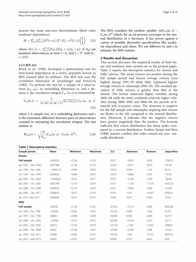
3 Results and discussionThis section discusses the empirical results of both lin-ear and nonlinear tests carried out in the present paper.Table 1 reports the descriptive statistics for Sensex andNifty returns. The mean returns are positive during thefull sample period and Sensex average returns werehighest during 1991–93 while Nifty registered highestaverage returns in subsample 2003–05. The standard de-viation of Nifty returns is greater than that of theSensex. The former witnessed higher volatility during2006–08 while the latter exhibited relatively higher vola-tility during 2000–2002 and 2006–08, the periods of fi-nancial and economic crises. The skewness is negativefor the full sample and subsamples implying that returnsare flatter to the left compared to the normal distribu-tion. Moreover, it indicates that the negative returnshave greater magnitude than the positive. The kurtosisindicates that return distribution has sharp peaks com-pared to a normal distribution. Further, Jarque and Bera(1980) statistic confirm that index returns are non- nor-mally distributed.

Table 1 Descriptive statistics

Sample period Mean Minimum Maximum S.D Skewness Kurtosis Jaqua-Bera

Sensex

Full sample 0.000553 −0.136 0.159 0.017 −0.042 5.893 7780.03

Jan 1991 – Dec 1993 0.001988 −0.136 0.123 0.024 −0.047 4.624 541.93

Jan 1994 - Dec 1996 −0.000116 −0.046 0.056 0.014 0.454 1.229 68.16

Jan 1997 – Dec 1999 0.000656 −0.086 0.073 0.018 −0.086 2.091 135.45

Jan 2000 – Dec 2002 −0.000525 −0.074 0.071 0.017 −0.338 2.165 160.65

Jan 2003 – Dec 2005 0.001348 −0.118 0.079 0.013 −1.139 11.120 4075.26

Jan 2006 – Dec 2008 0.000035 −0.116 0.079 0.021 −0.344 2.584 222.00

Jan 2009 – Dec 2011 0.000635 −0.075 0.159 0.016 1.291 14.567 6766.81

Jan 2012- Mar 2013 0.000699 −0.027 0.026 0.009 0.077 0.580 5.014

Nifty

Full sample 0.00035 −0.130 0.163 0.0162 −0.122 6.428 8262.46

Jan 1994 - Dec 1996 −0.0002 −0.043 0.054 0.0139 0.498 1.456 92.78

Jan 1997 – Dec 1999 0.0006 −0.088 0.099 0.0098 0.009 3.680 422.17

Jan 2000 – Dec 2002 −0.0004 −0.072 0.072 0.0160 −0.244 2.652 227.11

Jan 2003 – Dec 2005 0.0012 −0.130 0.079 0.0139 −1.407 12.870 5488.81

Jan 2006 – Dec 2008 0.0001 −0.130 0.067 0.0209 −0.530 3.298 372.82

Jan 2009 – Dec 2011 0.0006 −0.063 0.163 0.0156 1.403 15.912 8078.16

Jan 2012 – Mar 2013 0.0007 −0.027 0.027 0.0091 0.079 0.643 6.09


3.1 Linear dependenceThe present study employs Ljung-Box test to checkwhether all autocorrelations are simultaneously equal tozero. The full samples of both the Sensex and Nifty pos-sess autocorrelations indicating dependence in stockreturns. The LB statistics are significant at 1 per cent levelshowing autocorrelations in the first two sub-periods.Nevertheless, stock returns in the last three subsamplesfollow a random walk. Interestingly, stock returns exhibitindependence during 1997–1999 and 2000–2002, theyears of Asian currency crisis and dot.com crash. The re-sults for Nifty indicate first order autocorrelation in thefirst four subsamples except 1997–1999 and thus suggestthe possibility of predictability of returns. Similar to thatof Sensex, the results for Nifty during 2006–2008, 2009–2011 and 2012–2013 show no autocorrelations suggestingindependence of returns. The runs tests statistics pre-sented in the last column of Table 2 are significant at 1per cent level and the negative values of Z for both Sensexand Nifty indicate positive correlation. The results showthat during the first five subsamples, the null of the ran-dom walk is rejected with the exception in 1997–1999.The runs test results for the last three subsamples show

no evidence of autocorrelation. We find no linear autocor-relations during those periods in which the major eventsnamely, the East Asian financial crisis, dot.com bubbleburst, and sub-prime mortgage crisis occurred. The auto-correlation and runs test results indicate that the Indianstock market is switching between efficiency and ineffi-ciency. In other words, these results seem to support theview that Indian stock market is adaptive.Furthermore, Lo and MacKinlay variance ratios at all

the chosen investment horizons (q) for Sensex and Niftyduring the full sample are greater than unity and statisti-cally significant at 1 percent level, indicating returns donot follow a random walk (Table 3). Nevertheless, vari-ance ratio statistics at any investment horizon in all thesubsamples are insignificant indicating independence ofreturns in these sub-periods. The sequential procedureof Lo and MacKinlay (1988) test leads to size distortionsand the test ignores the joint nature of random walk. Toovercome this problem, The Chow-Denning test, statisti-cally superior to individual variable ratio test, indicatespredictability of stock returns in India by rejecting nullof random walk over the whole sample at 5 per centlevel of significance. However, every subsample providesevidence of the independence of returns. The individualand multiple variance ratio results suggest that the Indianmarket is largely efficient surrounded by brief periods ofpredictability which disappear because information quicklybegins to reflect in returns and market moves towards effi-ciency again.The trends in linear test statistics help to examine the

magnitude of linear dependence during the sample

period (Figure 1). For Sensex, LB statistics witness sharpupward and downward spikes during the sample period.The test statistics were highest during 1994–1996 and2003–2005. Notwithstanding, the LB Q statistics started

Table 2 LB Q and runs tests statistics

Sample periods LB (5) LB (15) LB (20) Runs Z Statistics

Sensex

Full sample −0.001 0.024 −0.023 −6.385*

(46.45)* (75.99)* (96.84)*

Jan 1991 – Dec 1993 0.086 0.113 0.055 - 3.528*

(21.04)* (52.22)* (60.94)*

Jan 1994 - Dec 1996 0.015 0.011 −0.052 - 4.236

(38.39)* (48.20)* (50.89)*

Jan 1997 – Dec 1999 −0.050 −0.020 −0.046 −1.842

(3.73) (17.04) (22.41)

Jan 2000 – Dec 2002 −0.022 0.006 −0.094 - 2.611*

(6.34) (14.42) (31.77)**

Jan 2003 – Dec 2005 −0.032 −0.056 0.010 - 2.358*

(26.58)* (35.45)* (44.28)*

Jan 2006 – Dec 2008 −0.017 0.011 −0.049 - 1.3356

(7.60) (15.23)

Jan 2009 – Dec 2011 −0.055 0.002 −0.081 - 0.439

(6.65) (17.41) (31.47)**

Jan 2012 – Mar 2013 −0.008 0.009 0.024 - 0.929

(2.15) (12.78) (22.54)

Nifty

Full sample −0.008 0.001 −0.042 - 5.765*

(34.69)* (60.71)* (91.60)*

Jan 1994 - Dec 1996 0.030 0.003 −0.020 - 5.161*

(44.35)* (57.73)* (59.53)*

Jan 1997 – Dec 1999 0.002 −0.016 0.009 - 0.052

(0.267) (14.35) (23.68)

Jan 2000 – Dec 2002 0.016 0.013 −0.107 - 2.962*

(12.74)** 21.02 38.90*

Jan 2003 – Dec 2005 −0.037 −0.059 0.013 - 2.270**

37.46* 55.30* 61.54*

Jan 2006 – Dec 2008 −0.011 0.026 −0.066 - 1.105

4.81 24.02 31.58**

Jan 2009 – Dec 2011 −0.060 −0.006 −0.006 0.0367

4.98 16.93 29.14

Jan 2012 – Mar 2013 0.000 0.005 0.017 −0.874

2.69 14.66 21.51

The autocorrelation coefficient followed by Ljung-Box (LB) Q statistics inparenthesis are given in the table at lags 5, 15 and 20 for the full sample andsubsample period. The null of LB is zero autocorrelation. The last columnfurnishes the Runs Z statistics. * and ** denote the significance level at 1%and 5% respectively.


moving downward from 2006 including the periods ofsub-prime mortgage crisis and global economic melt-down of 2008. The trends in runs statistics exhibit simi-lar patterns. The Lo-MacKinlay and Chow-Denningstatistics show that the magnitude of linear dependence

is highest during the first two subsamples, 1994–1996,1997–1999. Thereafter, the trend in test statistics mov-ing downwards, and values are insignificant indicatingno predictability of returns based on past returns. Thetrends in magnitude of linear dependence in Nifty

Table 3 Variance ratio test statistics

Sample periods Lo-MacKinlay variance ratios for investment horizons (q) Chow andDenning statistic2 4 8 16

Sensex

Full sample 1.08* 1.12* 1.12*** 1.19** 3.767**

(3.767) (2.878) (1.868) (2.071)

Jan 1991 – Dec 1993 1.11 1.20 1.26 1.42 1.066

(1.066) (1.083) (0.910) (1.001)

Jan 1994 - Dec 1996 1.21 1.27 1.32 1.21 0.772

(0.772) (0.567) (0.424) (0.196)

Jan 1997 – Dec 1999 1.04 1.08 1.03*** 1.06 0.291

(0.291) (0.292) (0.082) (0.094)

Jan 2000 – Dec 2002 1.06 1.09 1.10 1.11 0.391

(0.391) (0.298) (0.211) (0.163)

Jan 2003 – Dec 2005 1.08 1.02 1.08 1.15 0.271

(0.273) (0.052) (0.104) (0.129)

Jan 2006 – Dec 2008 1.07 1.07 0.985 1.05 0.653

(0.653) (0.346) (−0.045) (0.124)

Jan 2009 – Dec 2011 1.06 1.06 1.01 1.09 0.319

(0.319) (0.172) (0.022) (0.117)

Jan 2012 – Mar 2013 0.98 1.06 1.10 1.10 0.012

(−0.01) (0.023) (0.024) (0.018)

Nifty

Full sample 1.07* 1.08** 1.06 1.10 3.180*

(3.180) *(1.896) (1.071) (1.121)

Jan 1994 - Dec 1996 1.23 1.31 1.40 1.25 1.055

(1.055) (0.789) (0.673) (0.304)

Jan 1997 – Dec 1999 1.00 0.99 0.96 0.96 0.003

(0.003) (−0.005) (−0.107) (−0.068)

Jan 2000 – Dec 2002 1.09 1.08 1.11 1.15 0.602

(0.602) (0.284) (0.260) (0.252)

Jan 2003 – Dec 2005 1.11 1.06 1.12 1.16 0.587

(0.586) (0.183) (0.218) (0.203)

Jan 2006 – Dec 2008 1.06 1.06 0.99 1.07

(0.677) (0.395) (−0.015) (0.216) 0.677

Jan 2009 – Dec - 2011 1.04 1.05 1.00* 1.07 0.288

(0.276) (0.172) (0.002) (0.112)

Jan 2012 – Mar 2013 0.97 1.06* 1.10** 1.12** 0.021

(−0.021) *(0.032) (0.035) (0.029)

Note: The Lo-MacKinlay variance ratios VR (q) are reported in the main rows and variance test [Z * (q)] statistics are given in parentheses. Under the null of randomwalk, the variance ratio value is expected to equal one. Chow-Denning heteroscedastic statistics are presented in the last column and the critical value is 2.49.*, ** and *** denote significance at 1%, 5% and 10% respectively.


returns are similar to that of Sensex. The linear test re-sults presented in Figure 1 indicate highest linear de-pendence in Nifty returns during subsample 1994–1996and 2003–2006. In the rest of the subsamples, the valuesare low showing no autocorrelation or linear depend-ence in Nifty returns. Overall, the magnitude of lineardependence has fallen over the period (Figure 1). Inother words, the results support that the Indian stockmarket has become efficient from the beginning of theyear 2003. It may be because of the fact that NSE hasbrought several changes in market microstructure andtrading practices, which BSE followed later. It seems thatthese changes along with financial sector reforms andregulatory measure of Securities and Exchange Boardof India (SEBI) have positively influenced the efficiencyin the market. Strikingly, linear test statistics are statis-tically insignificant during 1997–1999, 2000–02 and2006–2008, the periods of Asian financial crash, techboom burst and sub-prime mortgage crisis followed bya global recession respectively. The present evidence ofunpredictability of returns during crises is consistentwith Kim et al. (2011) who observed no predictabilityduring stock market crashes (1929 and 1987).

3.2 Nonlinearity in stock returnsThe linear tests such as autocorrelation, variance ratio,and runs tests are incapable to capture nonlinear pat-terns in the return series. The failure to reject linear de-pendence is insufficient to prove independence in viewof non-normality of the series (Hsieh 1989) and not ne-cessarily imply independence (Granger and Anderson1978). The presence of nonlinearity indicates predict-ability and potential excess profits to agents. The use oflinear models in such conditions may give the wronginference of unpredictability. Moreover, the presence ofnonlinearity in stock returns contradicts EMH. In thisstudy, we employed a set of nonlinear tests to inves-tigate the presence of nonlinear dependence. Beforeperforming these tests, the returns were corrected forheteroscadasticity and we removed linear dependencefitting an appropriate AR (ρ) model so that any re-maining dependence would be nonlinear. LB statisticsfor residuals extracted after filtering for linearity showno autocorrelation up to lag 20 for each subsample ofSensex and Nifty (Table 4).The McLoed-Li statistics prove that each subsample of

Sensex and Nifty has a nonlinear dependence except

Figure 1 Trends in linear tests statistics.


2012–13 and 2009–2013 subsamples. This indicates thatIndian stock market is inefficient during these sampleperiods and over the whole sample period. Further, Tsayand Engle LM tests show strong evidence of nonlinearbehaviour for both the full sample and subsamples atchosen lags (Table 5). Similar to McLeod-Li results, the

Tsay and Engle LM tests indicate unpredictability ofreturns during the last subsample (2012–13). Overall,the results presented in Tables 4 and 5 show a signifi-cant presence of nonlinearity in returns. This impliesthat Indian stock market was weakly inefficient through-out the sample period.

Table 4 McLeod-Li test statistics

Sample periods AR (ρ) LB (5) LB (15) LB (20) McLeod-Li statistic

Lag 5 Lag 15 Lag 20

Sensex

Full sample 9 0.043 0.748 26.32 988.6* 2130.1* 2415.5*

(1.000) (1.000) (0.155) (0.000) (0.000) (0.000)

Jan 1991 – Dec 1993 7 0.196 24.06 29.57 81.7* 238.0* 255.3*

(0.999) (0.064) (0.077) (0.000) (0.000) (0.000)

Jan 1994 - Dec 1996 2 4.745 16.94 19.14 47.17* 97.49* 130.53*

(0.447) (0.322) (0.512) (0.000) (0.000) (0.000)

Jan 1997 – Dec 1999 1 3.64 16.86 22.38 30.19* 41.84* 52.99*

(0.602) (0.327) (0.320) (0.000) (0.000) (0.000)

Jan 2000 – Dec 2002 2 3.161 11.00 26.48 187.69* 296.07* 329.56*

(0.675) (0.752) (0.150) (0.000) (0.000) (0.000)

Jan 2003 – Dec 2005 2 8.673 20.459 23.306 245.29* 263.26* 264.19*

(0.122) (0.155) (0.274) (0.000) (0.000) (0.000)

Jan 2006 – Dec 2008 2 2.349 18.209 23.168 277.27* 590.73* 671.05*

(0.798) (0.251) (0.280) (0.000) (0.000) (0.000)

Jan 2009 – Dec - 2011 1 6.263 18.81 23.67 4.712 29.28** 33.42**

(0.281) (0.222) (0.296) (0.451) (0.014) (0.030)

Jan 2012 – Mar 2013 0 2.152 12.788 22.546 1.550 15.00 27.79

(0.827) (0.618) (0.311) (0.907) (0.451) (0.114)

Nifty

Full sample 11 0.028 6.371 26.939 550.20* 964.60* 1066.23*

(1.000) (0.972) (0.137) (0.000) (0.000) (0.000)

Jan 1994 - Dec 1996 2 5.813 19.919 21.824 69.38* 154.97* 185.82*

(0.324) (0.175) (0.350) (0.000) (0.000) (0.000)

Jan 1997 – Dec 1999 0 0.267 14.356 23.686 23.72* 28.13** 49.47*

(0.998) (0.498) (0.256) (0.000) (0.020) (0.000)

Jan 2000 – Dec 2002 2 1.429 7.764 22.700 108.87* 199.44* 220.53*

(0.921) (0.932) (0.303) (0.000) (0.000) (0.000)

Jan 2003 – Dec 2005 2 8.715 21.42 28.444 286.24* 310.20* 311.07*

(0.157) (0.321) (0.099) (0.000) (0.000) (0.000)

Jan 2006 – Dec 2008 2 1.593 19.37 26.913 232.57* 441.67* 489.24*

(0.902) (0.197) (0.137) (0.000) (0.000) (0.000)

Jan 2009 – Dec - 2011 2 3.379 14.305 26.676 2.177 18.701 22.491

(0.641) (0.502) (0.144) (0.824) (0.227) (0.314)

Jan 2012 – Mar 2013 0 2.697 14.663 21.516 2.667 16.101 30.169***

(0.746) (0.475) (0.367) (0.751) (0.375) (0.067)

The autocorrelation coefficient followed by The Ljung-Box (LB) Q statistics in parenthesis are given in the table at lags 5, 15 and 20 for the full sample andsubsample period. *, ** and *** denote significance at 1%, 5% and 10% respectively.


The H statistics reject null of pure noise for Sensexand Nifty in all the subsamples with the exception ofsubsample 2012–2013 (Table 5). This exposes nonlinearcharacteristics of Indian stock returns during these pe-riods. Finally, the BDS statistics support evidence ofnonlinear dependence during the subsamples and fullsample for both the indices (Table 6). The rejection for

residuals from AR (ρ) indicates presence of nonlineardependence and implies the possible predictability of fu-ture returns using the history of returns.The trends in McLeod-Li show stronger presence of

nonlinear dependence in Sensex and Nifty returns dur-ing subsamples 2003–2005 and 2006–2008 (Figure 2).Again, the trends in Engle LM, Tsay, H and BDS test

Table 5 Tsay, Engle LM and H statistics

Sample period AR (ρ) Tsay F statistic Engle LM statistic H statistic

Lag 5 Lag 15 Lag 20 Lag 5 Lag 15 Lag 20

Sensex

Full sample 9 7.862* 3.613* 3.039* 564.1* 729.5* 758.2* 3760.9*

(0.000) (0.000) (0.000) (0.000) (0.000) (0.000) (0.000)

Jan 1991 – Dec 1993 7 2.837* 1.907* 1.786* 54.8* 101.2* 110.5* 405.6*

(0.000) (0.000) (0.000) (0.000) (0.000) (0.000) (0.000)

Jan 1994 - Dec 1996 2 1.858* 1.273** 1.282** 32.4* 50.5* 74.9* 139.7*

(0.000) (0.041) (0.016) (0.000) (0.000) (0.000) (0.000)

Jan 1997 – Dec 1999 1 2.436* 1.686* 1.457* 28.86* 37.5* 47.7* 183.9*

(0.001) (0.000) (0.000) (0.000) (0.001) (0.005) (0.000)

Jan 2000 – Dec 2002 2 2.396* 2.433* 2.168* 110.67* 138.8* 148.9* 364.8*

(0.002) (0.000) (0.000) (0.000) (0.000) (0.000) (0.000)

Jan 2003 – Dec 2005 2 6.609* 2.257* 1.910* 268.96* 272.2* 272.3* 721.7*

(0.000) (0.000) (0.000) (0.000) (0.000) (0.000) (0.000)

Jan 2006 – Dec 2008 2 4.734* 2.746* 2.667* 153.7* 179.4* 181.7* 680.9*

(0.000) (0.000) (0.000) (0.000) (0.000) (0.000) (0.000)

Jan 2009 – Dec - 2011 1 1.24 2.50* 2.483* 4.9 22.8 24.3 242.9*

(0.229) (0.000) (0.000) (0.495) (0.088) (0.231) (0.000)

Jan 2012 – Mar 2013 0 0.560 1.558* 1.073 1.6 13.3 25.8 52.8

(0.903) (0.003) (0.359) (0.911) (0.576) (0.172) (0.198)

Nifty

Full sample 9 6.240* 2.877* 2.427* 352.20* 425.36 437.38* 1848.41*

(0.000) (0.000) (0.000) (0.000) (0.000) (0.000) (0.000)

Jan 1994 - Dec 1996 2 1.509 1.583* 1.436* 50.21* 77.758 92.62* 158.67*

(0.095) (0.000) (0.000) (0.000) (0.000) (0.000) (0.000)

Jan 1997 – Dec 1999 0 2.842* 1.687* 1.295** 24.21* 27.85** 51.658* 157.77*

(0.000) (0.000) (0.011) (0.000) (0.022) (0.000) (0.000)

Jan 2000 – Dec 2002 2 1.852** 2.173* 1.949* 79.97* 126.46* 130.54* 380.80*

(0.024) (0.000) (0.000) (0.000) (0.000) (0.000) (0.000)

Jan 2003 – Dec 2005 2 6.757* 2.413* 1.985* 315.46* 320.34* 321.86* 799.69*

(0.000) (0.000) (0.000) (0.000) (0.000) (0.000) (0.000)

Jan 2006 – Dec 2008 2 5.583* 2.705* 2.459* 125.40* 152.41* 158.98* 663.08*

(0.000) (0.000) (0.000) (0.000) (0.000) (0.000) (0.000)

Jan 2009 – Dec - 2011 2 0.873 2.313* 2.268* 2.023 15.292 16.87 195.63*

(0.593) (0.000) (0.000) (0.845) (0.430) (0.661) (0.000)

Jan 2012 – Mar 2013 0 0.489 1.577* 1.181 2.931 14.672 27.786 56.255

(0.945) (0.003) (0.193) (0.710) (0.475) (0.114) (0.121)

*,** denote 1% and 5% significance level.


statistics are low indicating lesser magnitude of nonlin-ear dependency in stock returns till the year 2000 andthereafter returns exhibit increasing nonlinear tendencyreaching peak during subsample, 2006–2008. The sub-sample 2006–2008 that possess pockets of strong pres-ence of nonlinear dependence is associated with sub-prime mortgage and global financial crisis (2008). Inpost 2008 subsample, however, all the test statistics sug-gest relatively weaker presence of nonlinear dependencein returns (See, Figure 2).The foreign portfolio investments help emerging mar-

kets by offering quality information and liquidity and in-fluence efficiency. Nevertheless, the yield sensitive FIIsfly from emerging markets in response to global news orloss of confidence in the economy. We find interestingassociation between nonlinear dependence and FIIs inIndia. We find net outflow of FIIs from Indian stockmarket creating panic in the market during financial cri-ses of 1997–98, 2000–01 and 2007–08 and during theseperiods, we find statically significant nonlinearity instock returns (Figure 3). The external events thus influ-ence the behaviour of returns in emerging markets. Over-all, we find a strong evidence of nonlinearity throughoutthe sample period in Indian market. Although we find evi-dence of an increasing nonlinear dependence, it is taper-ing off in most recent subsamples.

The linear test results support the proposition that In-dian stock market switched between efficient and ineffi-cient periods and this finding is consistent with Charleset al. (2012) Kim et al. (2011), and Alvarez-Ramirez et al.(2012). Nevertheless, the present evidence of strong pres-ence of nonlinear dependence in stock returns throughoutthe sample suggests that the Indian stock market still inef-ficient and not experienced efficiency yet. Our finding ofhighest magnitude of nonlinearity during periods of finan-cial crises in Indian stock returns is consistent with thefindings of Urquhart and Hudson (2013) who found simi-lar evidence for the US market. The evidence of nonline-arity during financial crises shows that the stock marketcrash and economic crises negatively affect the stock mar-ket efficiency. Furthermore, the present study finds out-flow of FIIs during global financial crises. This evidencesuggests that the increasing integration of Indian capitalmarket has not only brought the benefits but also exposedthe market to external shocks.

4 Summary and conclusionThe present paper has investigated the adaptive markethypothesis (AMH) in India, one of the fastest growingmarkets. The linear test results indicated a cyclical patternin autocorrelations suggesting that the Indian stock mar-ket switched between periods of efficiency and inefficiency

Table 6 BDS test statistics

Sample period AR (ρ) m = 2, ε = 0.75s m = 4, ε = 1.0s m = 8, ε =1.25 S m= 10, ε = 1.50s

Sensex

Full sample 9 17.65* (0.000) 27.88* (0.000) 42.94*(0.000) 44.24* (0.000)

Jan 1991 – Dec 1993 7 3.74* (0.000) 4.42*(0.000) 6.33*(0.000) 7.40*(0.000)

Jan 1994 - Dec 1996 2 5.76* (0.000) 8.24* (0.000) 11.66* (0.000) 12.21*(0.000)

Jan 1997 – Dec 1999 1 3.00* (0.002) 4.52* (0.000) 6.30*(0.000) 6.95* (0.000)

Jan 2000 – Dec 2002 2 8.46*(0.000) 13.08*(0.000) 18.11*(0.000) 19.20*(0.000)

Jan 2003 – Dec 2005 2 3.85* (0.000) 5.60* (0.000) 9.01*(0.000) 9.77* (0.000)

Jan 2006 – Dec 2008 2 9.08* (0.000) 14.26*(0.000) 24.40*(0.000) 23.56*(0.000)

Jan 2009 – Dec - 2011 1 3.85* (0.000) 7.40*(0.000) 12.98* (0.000) 14.11* (0.000)

Jan 2012 – Mar 2013 0 −0.71* (0.474) 0.306* (0.759) 1.893* (0.058) 2.288* (0.022)

Nifty

Full sample 11 15.15* (0.000) 23.89 (0.000) 35.94 (0.000) 37.65 (0.000)

Jan 1994 - Dec 1996 2 5.322* (0.000) 8.534* (0.000) 11.33* (0.000) 11.73* (0.000)

Jan 1997 – Dec 1999 0 2.149* (0.031) 4.081* (0.000) 5.351* (0.000) 5.808* (0.000)

Jan 2000 – Dec 2002 2 8.08* (0.000) 12.14* (0.000) 15.28* (0.000) 15.59* (0.000)

Jan 2003 – Dec 2005 2 4.67* (0.000) 6.43* (0.000) 9.68* (0.000) 10.89* (0.000)

Jan 2006 – Dec 2008 2 8.63* (0.000) 13.89* (0.000) 23.71* (0.000) 22.49* (0.000)

Jan 2009 – Dec - 2011 2 3.73* (0.000) 6.61* (0.000) 12.02* (0.000) 12.97* (0.000)

Jan 2012 – Mar 2013 0 −1.05 (0.292) 0.288 (0.772) 1.732 (0.083) 2.905 (0.004)

Here, ‘m’ and ‘ε’ denote the embedding dimension and distance, respectively and ‘ε’ equal to various multiples (0.75, 1, 1.25 and 1.5) of standard deviation (scp ofthe data. The value in the first row of each cell is a BDS test statistic followed by the corresponding p-value in parentheses. The asymptotic null distribution of teststatistics is N (0.1). Asterisked values indicate 1% level of significance.


and market has become efficient from the year 2003.The findings from each of the nonlinear tests suggest astrong presence of nonlinear dependence in Indianstock returns throughout the sample period implyingpossible predictability of returns and consequent excessreturns. The nonlinearity in stock returns was highestduring various financial crises originated outside Indiaand this finding shows association of informational ineffi-ciency and financial crises. Furthermore, the vulnerability

of Indian stock market to the external shocks in a finan-cially liberalized economy is evident from the outflow ofFIIs owing to external events. The present evidence of in-fluence of financial crises and reversal of FIIs on efficiencyof stock market should be interpreted as identifying an as-sociation rather than causality.The reforms initiated have positive influence on stock

market is evident from the fall in magnitude of nonlineardependence in recent periods. The present study finds

Figure 2 Trends in nonlinear tests statistics.

Figure 3 Foreign institutional investments in Indian stock market.


that Indian stock market is still evolving and not fullyadaptive, as it has not gone through a single period of ef-ficiency. The linear independence and weaker presenceof nonlinear dependence in returns from 2009 is suffi-cient to conclude that Indian stock market is moving to-wards efficiency. The present finding of an increasedpossibility of predictability during financial crises andlarge outflow of investment calls for appropriate policymeasures to address the external shocks and retain theconfidence of foreign investors.

EndnotesaThe seminal work of Bachelier (1900) laid theoretical

foundation for the theory of efficient market. The pio-neering work of Samuelson (1965) added rigour to thetheory of stock market efficiency.

bMalkiel (1973) writes to the extent that ‘a blind-folded chimpanzee throwing darts at the Wall Streetcould select a portfolio that would do as well as theexperts’.

cCampbell et al. (1997) note that testing of marketefficiency as a condition of all or nothing is not use-ful and such an efficient market is the economicallyunrealizable ideal market. They suggest relative efficiencybecause measuring efficiency provides more insights thantesting it.

dA rolling sample is an alternative method used in em-pirical literature to examine evolving nature. However,an event may squeeze or influence the overall results.Hinich and Patterson (1995) suggested a windowed ap-proach. We did not find any optimization benefits inusing rolling sample in the present context.

eHinich and Patterson in their unpublished work of1995 recommend c = 0.4. The same is followed here.

Competing interestsWe hereby declare that we do not have any financial or non-financialcompeting interests to disclose.

Authors’ contributionsGSH carried out the study on stock returns predictability and adaptivemarket hypothesis and developed conceptual framework, while JK finds outassociated events with the efficiency through extensive survey of reports.Both GSH and JK contribute in the methodology section. In addition, bothproof read the paper thoroughly and edited the manuscript. GSHincorporated the suggestions of conference participants. JK modified thewhole research as per the guidelines of the Springer Plus. Both the authorsread and approved the final manuscript.

AcknowledgementsWe thank the participants of Fourth International Conference on AppliedEconometrics held on March 20 & 21, 2014 at IBS Hyderabad, India for theuseful suggestions. Usual disclaimer applies.

Received: 20 July 2014 Accepted: 28 July 2014Published: 12 August 2014

ReferencesAlvarez-Ramirez J, Rodriguez E, Espinosa-Paredes G (2012) Is the US stock market

becoming weakly efficient over time? Evidence from 80-year-long data.Phys A 391:5643–5647

Amanulla S, Kamaiah B (1998) Indian stock market: is it informationally efficient?Prajnan 25:473–485

Bachelier L (1900) Theory of Speculation. PhD Thesis, Faculty of the Academyof Paris

Barua SK (1981) The short run price behaviour of securities: some evidence onefficiency of Indian capital market. Vikalpa 16:93–100

Brock WA, Sheinkman JA, Dechert WD, LeBaron B (1996) A test forindependence based on the correlation dimension. Econom Rev15:197–235

Campbell JY, Lo AW, MacKinlay AC (1997) The Econometrics of financial markets.Princeton, New Jersey

Charles A, Darne O, Kim H (2012) Exchange-rate predictability and adaptivemarket hypothesis: evidence from major exchange rates. J Int MoneyFinanc 31:1607–1626

Chow KV, Denning KC (1993) A simple multiple variance ratio test. J Econom58:385–401

Engle RF (1982) Autoregressive conditional heteroskedasticity with estimatesof the variance of United Kingdom inflation. Econom 50:987–1007

Fama EF (1970) Efficient capital markets: a review of theory and empirical work.J Finance 25:383–417

Granger CWJ, Anderson AP (1978) An introduction to bilinear time series models.V & R, Gottingen

Grassberger P, Procaccia I (1983) Characterization of strange attractors. Phys RevLett 50:346–340

Hinich MJ (1996) Testing for dependence in the input to a linear time seriesmodel. J Non-paramet Stat 6:205–221

Hinich MJ, Patterson DM (1995) Detecting epochs of transient dependence inwhite noise. University of Texas, Mimeo

Hiremath GS, Kamaiah B (2010) Some further evidence on behaviour of stockreturns in India. Int J Econ Financ 2:157–167

Hiremath GS, Kamaiah B (2012) Variance ratios, structural breaks and non-random walk behaviour in the Indian stock returns. J Econ Bus Stud18:62–82

Hsieh DA (1989) Testing for nonlinear dependence in daily foreign exchangerates. J Buss 62(3):339–368

Ito M, Sugiyama S (2009) Measuring the degree of time varying marketinefficiency. Econ Lett 103:62–64

Jarque CM, Bera AK (1980) Efficient test of normality, homoscedasticity andserial independence of regression residuals. Econ Lett 6:255–259

Kim JH, Shamsuddin A, Lim KP (2011) Stock returns predictability and theadaptive markets hypothesis. Evidence from century long U.S. data. J EmpiriFinanc 18:868–879

Ljung GM, Box GEP (1978) On a measure of lack of fit in time series models.Biom 65:297–303

Lo AW (2004) The adaptive markets hypothesis: market efficiency from anevolutionary perspective. J Portf Manag 30:15–29

Lo AW (2005) Reconciling efficient markets with behavioral finance: the adaptivemarkets hypothesis. J Invest Consult 7:21–44

Lo AW, MacKinlay AC (1988) Stock market prices do not follow randomwalks: evidence from a simple specification test. Rev Financ Studies1:41–66

Malkiel BG (1973) A random walk down Wall Street. W. W, Norton & Co,New York

McLeod AI, Li WK (1983) Diagnostic checking ARMA time series models usingsquared-residual autocorrelations. J Time Ser Anal 4:269–273

Noda A (2012) A test of the adaptive market hypothesis using non-Bayesiantime-varying AR model in Japan. http://arxiv.org/abs/1207.1842. Accessed on25 January 2013

Poshakwale S (2002) The random walk hypothesis in the emerging Indian stockmarket. Journal of Bus Financ & Account 29:1275–1299

Rao KN, Mukherjee K (1971) Random walk hypothesis: an empirical study.Arthaniti 14:53–58

Samuelson P (1965) Proof that properly anticipated prices fluctuate randomly. IndManag Rev 6:41–49

Sharma JL, Kennedy RE (1977) A comparative analysis of stock price behavior onthe Bombay, London, and New York stock exchanges. J Financ QuantAnalysis 12:391–413


Standard and Poor’s (2012) Global stock market fact book. Standard and Poorscorporation, New York

Tsay RS (1986) Nonlinearity tests for time series. Biom 73:461–466Urquhart A, Hudson R (2013) Efficient or adaptive markets? Evidence from

major stock markets using very long historic data. Int Rev Financ Anal28:130–142

doi:10.1186/2193-1801-3-428Cite this article as: Hiremath and Kumari: Stock returns predictabilityand the adaptive market hypothesis in emerging markets: evidencefrom India. SpringerPlus 2014 3:428.

Submit your manuscript to a journal and benefi t from:

7 Convenient online submission

7 Rigorous peer review

7 Immediate publication on acceptance

7 Open access: articles freely available online

7 High visibility within the fi eld

7 Retaining the copyright to your article

Submit your next manuscript at 7 springeropen.com


munich personal repec archive - uni- · pdf file0 3 5 $ munich personal repec archive stock...

Documents