MPRAMunich Personal RePEc Archive

The growth trade-off between direct andindirect taxes in South Africa: Evidencefrom a STR model

Andrew Phiri

Department of Economics, Finance and Business Studies, CTIPotchefstroom Campus, North West, South Africa

1 February 2016

Online at https://mpra.ub.uni-muenchen.de/69152/MPRA Paper No. 69152, posted 3 February 2016 05:36 UTC

The growth trade-off between direct and indirect taxes in South Africa: Evidence from

a STR model

A. Phiri

Department of Economics, Finance and Business Studies, CTI Potchefstroom Campus,

North West, South Africa

ABSTRACT: The tax system forms the backbone to the functioning of the South African fiscal

authorities and it is has been recently questioned whether alterations in the existing tax mix

could promote economic growth. Using quarterly data from 1990:Q1 and 2015:Q2, this study

investigated the effects of direct and indirect taxes on economic growth for South Africa using

the recently developed smooth transition regression (STR) model. Our findings suggest an

optimal tax of 10.27 percent on the indirect tax–growth ratio, of which below this rate indirect

taxes are positively related with economic growth whereas direct taxes are negatively related

with growth. Above the optimal tax rate, taxation bears no significant relationship with

economic growth. We therefore suggest that policymakers place a greater burden on indirect

taxes and yet ensure that the contribution of indirect taxes to economic growth does not exceed

the threshold of 10.27 percent.

Keywords: Direct taxes; Indirect taxes; optimal tax; VAT; Economic growth, South Africa,

Smooth transition regression (STR) model.

JEL Classification Code: C22, C51, H21, H30, O4.

1 Introduction

In wake of the global financial crisis of 2007-2009, most economies worldwide are in

their recovery phases in the aftermath following the collapse of the US financial system. The

global financial crisis took a major toll on key macroeconomic performance indices in countries

across the globe with South Africa bearing no exception to this rule. In attempts to boost

economic growth, policymakers worldwide are focusing on tax reform policy as a vehicle

towards attaining this goal. For the specific case of South Africa, speculation has run high

concerning local government plans to increase government expenditure by shifting the burden

from direct taxes (i.e. personal income and corporate taxes) to indirect taxes (i.e. value added

tax (VAT)). Apparently this tax reform policy comes recommended by the Davis Tax

Committee and so far, these reforms have been advocated for based on two primary arguments.

Firstly, it is contended that the current structure of the tax system in the country cannot foster

higher economy growth due to heavy reliance on corporate and income taxes. In other words,

if policymakers were to continue relying on direct taxes for purposes of increasing government

revenue, then such tax increases would exert adverse effects on economic growth. Secondly,

by increasing indirect taxes, less tax burden will be borne by individuals and corporations thus

creating a conducive climate for domestic savings and foreign investments in the country.

Given the relative importance which tax policy plays towards economic development,

a number studies have taken the initiative of investigating the trade-off effects of taxes on

economic growth for South Africa. To the best of our knowledge, there have been four case

studies conducted thus far for South Africa and these are the works of de Wet et. al. (2005),

Koch et. al. (2005), Schoeman and van Heerden (2009) and Saibu (2015). Collectively, these

studies rely on a wide range of econometric methods applied to empirical data. For instance,

de Wet et. al., (2005) estimate an augmented neo-classical growth model using OLS estimators;

Koch et. al. (2005) use a two-stage Data Envelopment Analysis (DEA) to estimate an

augmented neo-classical growth model; whereas Schoeman and van Heerden (2009) and Saibu

(2015) make use of OLS in estimating Scully’s (1996, 2000) tax-optimizing model. Overall,

the consensus drawn over these studies points to a negative tax-growth relationship for the

South African economy. Whilst these studies provide a good basis for investigating the tax-

growth relationship in South Africa, we observe that the authors’ use of linear estimation in

their empirical analysis leaves the studies prone to criticisms of not addressing possible

nonlinear relations existing between the time series variables. This is a cause for genuine

concern given the increasing amount of evidence in the literature in support of nonlinear

dynamic structure of macroeconomic data. These nonlinear studies generally imply that the

conventional linear models are misspecified. Moreover, the time span covered by previous

South African studies encompasses a number of important political events and tax policy

reforms, which furthers the case for possible nonlinear relationships between time series of

economic variables.

In our study, we contribute to the literature by modelling nonlinear trade-off effects of

direct and indirect taxes on economic growth for South African using quarterly data collected

between 1990:Q1 and 2015:Q2. Theoretically, we follow in pursuit of De Wet et. al. (2005)

who augment Feder’s (1983) two-sector production function into a steady-state growth

estimation equation. Empirically, we rely on the newly developed smooth transition regression

(STR) framework in order to model out the nonlinear trade-off effects of direct and indirect

taxes on economic growth. Given the wide range of available nonlinear econometric models in

the literature, we consider the STR model as being most appropriate for the following reasons.

Firstly, the STR model encompasses other competing nonlinear econometric models such as

the threshold autoregressive (TAR), the Exponential Autoregressive (EAR) and the Markov-

Switching (MS) models, which are models that can be derived as extremities of the STR

regression. Secondly, the STR model assumes a smooth transition between regime coefficients

which is a feature of the econometric model which makes it theoretically appealing. Lastly, the

STR model allows the econometrician to choose both the appropriate switching variable and

the type of transition function unlike other regime-switching econometric models (Phiri, 2016).

Against this backdrop, we structure the remainder of the article as follows. The

literature review is presented in the next section of the paper. In the third section we outline the

methodology used in the study whereas the data and empirical results are given in the fourth

section. We conclude the study in the form of policy implications and possible avenues for

future work.

2 Literature Review

For simplicity sake, the current available literature on the tax-growth nexus can be

broadly segregated into two main strands of empirical works. First and foremost are those panel

data studies which make use of log-linear estimates of augmented transformations of Solow’s

(1965) neoclassical and Lucas’s (1988) endogenous growth models. Prominent examples of

pioneers belonging to this cluster of studies include Kormendi and Meguire (1985), King and

Rebelo (1990) and Barro (1990) who all set path for a wave of other empirical studies which

also relied on cross-sectional data for empirical use. For a greater part of it, these earlier panel

data studies reveal an inverse tax-growth relationship (e.g. Engen and Skinner (1992), Wright

(1996), Lee and Gordon (2005), Folster and Henrekson (2001) and Romero-Avila and Strauch

(2008)), even though some exceptional studies showed a positive relationship (e.g. Koester and

Kormendi (1989), Devaranjan et. al. (1996) and Agell et. al. (2006)) and a couple of other

papers have found no significant relationship between the variables (e.g. Levine and Renelt

(1992), Easterly and Rebelo (1993) and Mendoza et. al. (1994)).

A major criticism of the aforementioned studies lies in their inability to efficiently

account for cross-country differences in their empirical analysis. A perceptible demonstration

of this inefficiency is found for the US economy where the panel data studies of Koester and

Kormendi (1989) and Devaranjan et. al. (1996) advocate for a positive correlation between tax

and growth for panel data inclusive of US data whereas the single case studies of Mertens and

Ravn (2013), Barro and Redlick (2011) and Romer and Romer (2010) all find a negative tax-

growth relationship for the same country. Another issue which can be raised concerns the

failure of these studies to differentiate between distortionary and non-distortionary taxes. As is

discussed in Karagianni et. al. (2013), differentiating between distortionary and non-

distortionary forms of taxation is important because the use of average tax rates is an

inappropriate tax indicator due to it is strong correlation with public spending. To circumvent

this issue, researchers have opted to use a ‘tax structure mix’ as a means of measuring the effect

of tax policy on economic growth. This tax structure mix is combination of both direct and

indirect taxes which is used in the estimation of growth equations. So far the consensus drawn

from the literature is that corporate, income and other forms of direct taxes are more

distortionary towards economic growth whereas indirect taxes, such as VAT, are either

positively correlated or uncorrelated with growth (see Skinner (1987), Lee and Gordon (2005),

Arnold (2008), Widmalm (2009), Dackehag and Hansson (2012) and Bujang et. al. (2013)).

The second identifiable strand of empirical works in the literature vouch for a nonlinear

relationship between taxes and economic growth and this group of studies can be further sub-

divided into two groups. The first sub-group of studies are those who followed in pursuit of a

series of articles written by Scully (1995, 1996, 2000 and 2003) who developed both theoretical

and empirical specification for computing the optimal tax rate which results in growth

maximization. Belonging to this sub-group of studies are the works Chao and Grubel (1998),

Hill (2008), Keho (2010), Schoeman and van Heerden (2009) and Saibu (2015). We note that

Chao and Grubel (1998) estimate an optimal tax rate of 34 percent for Canadian data. On the

other hand, Hill (2008) estimates optimal tax rates ranging from 9 percent to 29 percent of GDP

across different states in the US. Meanwhile, Keho (2010) estimates an optimal tax rate of 22.3

percent for Ivory Coast using data collected between 1960 and 2006 whereas Saibu (2015)

estimates optimal tax rates for Nigerian as well as for South Africa for data collected between

1964 and 2012. For the former country the optimal rate is found to be 30 percent whereas for

the later the optimal rate is 15 percent. However, using data collected from 1960 to 2006,

Schoeman and van Heerden (2009) find an optimal tax rate of 21.94 percent for South Africa.

What is important to note is that the optimal tax rates documented in the literature differ, not

only across different countries, but also for the same country as can be witnessed in the study

of Van Heerden and Schoeman (2008) in comparison to that of Saibu (2015) for the case of

South Africa. Nevertheless, this particular sub-group of studies remains relevant to literature

seeing that they can be used to guide policymakers in amending discrepancies between the

current or prevailing tax-growth ratio and the estimated optimal tax-growth rate.

And even with the progressive nature of these studies in capturing the optimal level of

tax, the underlying empirical model has been further deemed as being flawed on account of

using a functional form which produces spurious estimates of the optimal level of tax (Hill,

2008 and Kennedy, 2000). This flaw lead to the emergence to the second sub-group of

nonlinear studies who empirically capture nonlinearity in the tax-growth relationship by

employing two measures of government tax in their growth equations, namely the ratio of tax

returns to GDP as well as the square of tax returns expressed as ratio of GDP. The former term

is intended to measure the tax-growth relationship at low tax levels whereas the later term

measures this relationship at high tax levels. Studies which have used to this method to quantify

nonlinearities in the tax-growth relationship include Dackehag and Hansson (2012), Stoilova

and Patonov (2013), Nantob (2014), and Hunady and Orvislea (2015). On one hand, the studies

of Dackehag and Hansson (2012) and Nantob (2014) show that low levels of tax are positively

correlated with economic growth whilst high levels of tax exert negative effects on growth. On

the other hand, the study of Stoilova and Patonov (2013) find that low tax rates hamper

economic growth whereas high levels of taxation are beneficial towards growth. Once again,

the inconclusiveness of the empirical studies is demonstrated and thus warrants further

deliberation into the subject.

3 Empirical Framework

Of recent, a growing number of sophisticated nonlinear econometric models have been

introduced into the academic literature. Among these models, is the smooth transition

regression (STR) model as introduced by Luukkonen et. al. (1988) and modified by Terasvirata

(1994). In comparison to other competing state-dependent non-linear time series models such

as the threshold autoregressive (TAR), Exponential Autoregressive (EAR) and the Markov

Switching (MS) models, the STR model holds a high level of appeal because unlike these other

nonlinear models the transition between regime states is endogenously determined.

Furthermore, the STR encompasses these other nonlinear econometric models. In its baseline

form, the STR model can be formulated as follows:

𝑦𝑡 = 𝛽0′ 𝑥𝑡 + 𝛽1

′𝑥𝑡 𝐺(𝑧𝑡; 𝜆, 𝑐) + 휀𝑡 t ~ iid N(0, h2t) (1)

Where yt is a scalar;𝛽0′ and 𝛽1

′ are parameter vectors; xt represents the vector of

explanatory variables, c is the transition variable , γ is the threshold estimate and G(zt; γ, c) is

a transition function which assumes the following logistic function:

𝐺(𝑧𝑡; 𝛾, 𝑐) =1

1+exp {−γ ∏ (𝑧𝑡−𝑐𝑘)}𝑘𝑘=1

(2)

Where zt is the transition or threshold variable whereas γ and c are the true threshold

estimate and the transition parameter, respectively. For empirical purposes we restrict the STR

model to the cases for k=1 (LSTR-1) and k=2 (LSTR-2). In firstly testing for linearity in

equation (1), we impose the constraint H0’: β1 = 0 on the regression. However, since the LSTR

model contains unidentified nuisance parameters under the null hypothesis of linearity,

conventional tests will produce nonstandard distributions (Davies, 1977). As suggested by

Luukkonen et. al. (1998), one method of circumventing this problem, involves replacing the

transition function G(zt; γ ,c) by its first order Taylor expansion around γ = 0, which results in

the following auxiliary function:

𝑦𝑡 = 𝜇𝑡 + 𝛽0′∗𝑥𝑡 + 𝛽1

′∗𝑥𝑡𝑧𝑡 + 𝛽2′∗𝑥𝑡𝑧𝑡

2 + 𝛽3′∗𝑥𝑡𝑧𝑡

3 + 휀𝑡∗ (3)

Where the parameter vectors 𝛽1∗, 𝛽2

∗, 𝛽3∗ are multiples of γ and 휀𝑡

∗=휀𝑡 + 𝑅3𝛽1′𝑥𝑡, with R3

being the remnant portion of the Taylor expansion. Hereafter, the null hypothesis of linearity

is tested as H0: β1 = β2 = β3 = 0 and this may tested via an LM test such that the Taylor series

does not affect asymptotic distribution theory. Once the null hypothesis of linearity is rejected,

one must decide on whether to fit an LSTR-1 or LSTR-2 model to the data. Terasvirta (1994)

suggests using a decision rule based upon a sequence of tests in equation (3). Particularly, the

author proposes testing the following null hypotheses:

I. 𝐻04∗ : 𝛽3

∗ = 0

II. 𝐻03∗ : 𝛽2

∗ = 0|𝛽3∗ = 0

III. 𝐻02∗ : 𝛽1

∗ = 0|𝛽3∗ = 𝛽2

∗ = 0.

The decision rule for selecting either a LSTR-1 or LSTR-2 model is thus as follows.

Select a LSTR-2 specification if 𝐻02∗ has the strongest rejection, otherwise, we select the LSTR-

1 specification. Once an appropriate LSTR specification has been chosen, the next step in the

modelling process is to obtain initial values for estimation purposes and these are obtained by

performing a grid search with a log-linear grid in γ and a linear grid in c. The starting values

are those which minimize the residual sum of squares (RSS) over the grid search and thereafter

the STR parameters are estimated by a nonlinear optimization routine that maximizes the log-

likelihood.

In turning to our theoretical model, we follow in pursuit of De Wet et. al. (2005) who

present an augmentation of Feder’s (1983) two-sector production function model for empirical

purposes. In particular, the authors exploit the possibility of government sector impacting

economic growth through two channels namely; through revenue collections and through

efficient allocation of resources. Their empirical growth model is specified as:

�̇�𝑌⁄ = 𝜃1[𝐼

𝑌⁄ ] + 𝜃2[�̇�𝐿⁄ ] + 𝜃3 [

�̇�𝑑𝑇

⁄ ] + 𝜃4 [�̇�𝑖𝑑

𝑇⁄ ] + [(𝛿

1 + 𝛿⁄ ) − 𝜃3] [�̇�𝑑

𝑌⁄ ] +

[(𝛿1 + 𝛿⁄ ) − 𝜃4] [

�̇�𝑖𝑑𝑌

⁄ ] + 휀𝑡 (4)

Where:

�̇�𝑌⁄ measures output growth (GDP).

𝐼𝑌⁄ measures the ratio of fixed capital formation to GDP.

�̇�𝐿⁄ measures the growth in the labour force.

�̇�𝑑𝑇

⁄ measures the growth in direct tax as a ratio of total taxes.

�̇�𝑖𝑑𝑇

⁄ measures the growth rate in indirect tax as a ratio of total taxes.

�̇�𝑑𝑌

⁄ measures the growth of direct taxes as a share of total income.

�̇�𝑖𝑑𝑌

⁄ measures the growth of indirect taxes as a share of total income.

The coefficients 𝜃1, 𝜃2, 𝜃3 and 𝜃4, measure the effects of investment on economic

growth, labour on economic growth, direct taxes on economic growth and indirect taxes on

economic growth, respectively. On the other hand, the coefficients [(𝛿1 + 𝛿⁄ ) − 𝜃3] and

[(𝛿1 + 𝛿⁄ ) − 𝜃4], are efficiency measures between direct taxes and the real economy as well

between indirect taxes and the real economy. If either [(𝛿1 + 𝛿⁄ ) − 𝜃3] > 0 or

[(𝛿1 + 𝛿⁄ ) − 𝜃4] > 0 occurs, then resources collected by the public sector are used more

efficiently by the government than the resources in the rest of the real sector (De Wet et. al.,

2005). The opposite is only possible if the coefficients 𝜃3 and 𝜃4 are of a greater absolute value

than the coefficients [(𝛿1 + 𝛿⁄ ) − 𝜃3] and [(𝛿

1 + 𝛿⁄ ) − 𝜃4]. In referring back to equations

(1) through (4), we can transform the linear growth regression (4) into the following STR

estimation model:

�̇�𝑌⁄ = 𝜃1[𝐼

𝑌⁄ ] + 𝜃2[�̇�𝐿⁄ ] + 𝜃3 [

�̇�𝑑𝑇

⁄ ] + 𝜃4 [�̇�𝑖𝑑

𝑇⁄ ] + [(𝛿

1 + 𝛿⁄ ) − 𝜃3] [�̇�𝑑

𝑌⁄ ] +

[(𝛿1 + 𝛿⁄ ) − 𝜃4] [

�̇�𝑖𝑑𝑌

⁄ ] +

𝜃1′ [𝐼

𝑌⁄ ] + 𝜃2′ [�̇�

𝐿⁄ ] + 𝜃3′ [

�̇�𝑑𝑇

⁄ ] + 𝜃4′ [

�̇�𝑖𝑑𝑇

⁄ ] + [(𝛿′

1 + 𝛿′⁄ ) − 𝜃3′ ] [

�̇�𝑑𝑌

⁄ ] + [(𝛿′

1 + 𝛿′⁄ ) −

𝜃4′ ] [

�̇�𝑖𝑑𝑌

⁄ ] × 𝐺(𝑧𝑡; 𝜆, 𝑐) +휀𝑡 (5)

Having formulated our estimation model, we thus outline the modelling and estimation

process of the formulated STR regression as follows. Firstly, we test linearity against the LSTR

alternative by using each of the explanatory variables as a possible transition variable. Once

linearity is rejected, we use the decision criteria to choose between LSTR-1 and LSTR-2

specification and choose the model with the highest rejection. Secondly, we carry out a three-

dimensional grid search over the values of zt, y and c for the STR regression. The optimal

values are the ones which minimize the residual sum of squares (RSS). Thirdly, we estimate

the chosen model using a Newton-Raphson algorithm to maximize the conditional maximum

likelihood function. Lastly, we perform diagnostic tests (i.e. ARCH effects, tests of no error

autocorrelation and parameter consistency) on the estimated model.

4 Data and Empirical Analysis

4.1 Data and unit root tests

For empirical purposes, we collect all our data from the South African Reserve Bank

(SARB) online database. Table 1 summarizes the raw time series as has been collected from

the SARB database. Each of the time series has been collected on quarterly basis between the

period of 1990:Q1 to 2015:Q2, that is with the exception of taxes on goods and services (VAT)

and the taxes on income, profits and capital gains, which have been collected on a monthly

basis from 1990:M1 to 2015:M6. Given the non-uniformity of the time series, we use cubic

spline interpolation to convert the monthly data (i.e. taxes on goods and services (VAT) and

the taxes on income, profits and capital gains) into quarterly data over the same sample period.

Table 1: Summary of time series

SARB code description of time series

KBP6006S Percentage change in gross domestic

product (�̇�𝑌⁄ )

KBP6282L Percentage change in ratio of gross fixed

capital formation to GDP (𝐼 𝑌⁄ )

KBP7008L Total employment in private sector (L)

KBP459M Total net national government tax revenue

(T)

KBP4578M National government tax revenue: taxes on

goods and services – value added tax (Tid).

KBP4578M National government tax revenue: total

taxes on income, profits and capital gains

(Td).

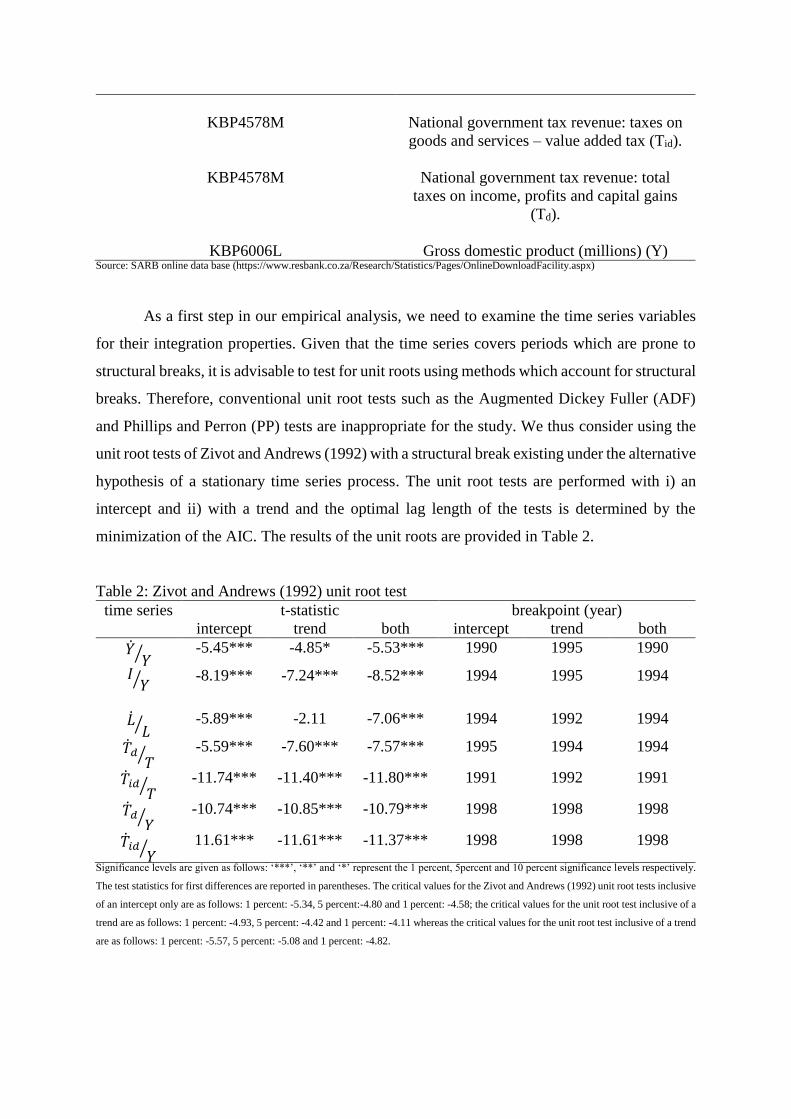
KBP6006L Gross domestic product (millions) (Y) Source: SARB online data base (https://www.resbank.co.za/Research/Statistics/Pages/OnlineDownloadFacility.aspx)

As a first step in our empirical analysis, we need to examine the time series variables

for their integration properties. Given that the time series covers periods which are prone to

structural breaks, it is advisable to test for unit roots using methods which account for structural

breaks. Therefore, conventional unit root tests such as the Augmented Dickey Fuller (ADF)

and Phillips and Perron (PP) tests are inappropriate for the study. We thus consider using the

unit root tests of Zivot and Andrews (1992) with a structural break existing under the alternative

hypothesis of a stationary time series process. The unit root tests are performed with i) an

intercept and ii) with a trend and the optimal lag length of the tests is determined by the

minimization of the AIC. The results of the unit roots are provided in Table 2.

Table 2: Zivot and Andrews (1992) unit root test

time series t-statistic breakpoint (year)

intercept trend both intercept trend both

�̇�𝑌⁄ -5.45*** -4.85* -5.53*** 1990 1995 1990

𝐼𝑌⁄

-8.19*** -7.24*** -8.52*** 1994 1995 1994

�̇�𝐿⁄ -5.89*** -2.11 -7.06*** 1994 1992 1994

�̇�𝑑𝑇

⁄ -5.59*** -7.60*** -7.57*** 1995 1994 1994

�̇�𝑖𝑑𝑇

⁄ -11.74*** -11.40*** -11.80*** 1991 1992 1991

�̇�𝑑𝑌

⁄ -10.74*** -10.85*** -10.79*** 1998 1998 1998

�̇�𝑖𝑑𝑌

⁄ 11.61*** -11.61*** -11.37*** 1998 1998 1998

Significance levels are given as follows: ‘***’, ‘**’ and ‘*’ represent the 1 percent, 5percent and 10 percent significance levels respectively.

The test statistics for first differences are reported in parentheses. The critical values for the Zivot and Andrews (1992) unit root tests inclusive

of an intercept only are as follows: 1 percent: -5.34, 5 percent:-4.80 and 1 percent: -4.58; the critical values for the unit root test inclusive of a

trend are as follows: 1 percent: -4.93, 5 percent: -4.42 and 1 percent: -4.11 whereas the critical values for the unit root test inclusive of a trend

are as follows: 1 percent: -5.57, 5 percent: -5.08 and 1 percent: -4.82.

Based on the unit root test results reported in Table 2, all observed time series, in their

levels, reject the null hypothesis of a unit root regardless of whether the unit root test regression

includes an intercept, a trend or both. An exception is warranted for the unit root tests

performed with trend on the growth in labour force variable. However, this is merely an

exceptional result than the norm. Another thing worth noting form the unit root test results

reported in Table 2 is that the various structural break points detected in the time series

correspond to the political shift of South Africa towards a democratic economy as witnessed

in 1994. Notably, the tax recommendations of the Katz commission where introduced and

implemented during the period of 1994 to 1998 which saw significant changes in the personal

income tax system. The detected structural breaks correspond to this period of tax reforms

within the country. All-in-all, we conclude that all utilized time series appear to be stationary

in their levels (i.e. integrated of order I(0)) and this satisfies a preliminary condition for

estimating the STR model without the fear of obtaining spurious regression results.

4.2 Selection, estimation and evaluation of STR model

Prior to the estimation of the STR model, we need to conduct linearity tests in order to

determine an appropriate transition variable for estimation usage. The purpose of the suggested

linearity tests is two-fold. Firstly, we use the linearity tests to inform us on which candidate

transition variable is most suitable for modelling nonlinear behaviour among the time series.

Secondly, we use the p-values from the linearity tests to determine whether the selected

transition variable should be used to model the STR regression as either an LSTR-1 or LSTR-

2 model. Pragmatically, we carry out the linearity tests by conducting a sequence of F-tests and

compute their corresponding p-values. The decision rule is to choose the model which produces

the lowest p-values. For the chosen model, we also conduct supplementary tests for no

remaining nonlinearity. The results of the linearity tests are reported in Table 3 whereas the

results of the tests for no remaining nonlinearity are presented in Table 4.

The linearity test results reported in Table 3 reveal that the null hypothesis of linearity

can be rejected for only two candidate variables, those being, the growth of direct taxes as a

share of total income (�̇�𝑑

𝑌⁄ ) and the growth of indirect taxes as a share of total income (

�̇�𝑖𝑑𝑌

⁄ ).

However, given smaller p-values associated with the growth of indirect taxes as a share of total

income (�̇�𝑖𝑑

𝑌⁄ ), we consider this time series the most suitable transition variable for building

our LSTR model. Also given that the F3 statistic produces the highest rejection associated with

the (�̇�𝑖𝑑

𝑌⁄ ) variable, we decide upon fitting an LSTR-1 to the data. Furthermore, the results of

the tests of no remaining linearity, as performed on the chosen LSTR-1 model and reported in

Table 4, shows no evidence of remaining nonlinearity for the regression model.

Table 3: Linearity tests

transition

variable

tests statistics Decision

F F4 F3 F2

𝐼𝑌⁄ 4.3438e-01 1.5583e-01 6.8692e-01 5.6340e-01 Linear

�̇�𝐿⁄

3.6582e-01 2.8636e-01 2.4223e-01 6.7763e-01 Linear

�̇�𝑑𝑇

⁄ 1.8651e-01 7.4984e-01 2.3839e-01 5.8844e-02 Linear

�̇�𝑖𝑑𝑇

⁄ 2.9371e-01 8.2546e-01 6.7247e-01 2.6595e-02 Linear

�̇�𝑑𝑌

⁄ 2.7808e-03 4.0006e-03 5.7885e-02 3.0139e-01 LSTR(1)

�̇�𝑖𝑑𝑌

⁄ 1.4412e-02 3.2655e-02 6.2697e-01 1.6723e-02 LSTR(1)#

Note: The F-tests for nonlinearity are performed for each possible candidate of the transition variable and the variable with the strongest test rejection (i.e. the smallest p-value)

is tagged with symbol #.

Table 4: Tests of no remaining nonlinearity

F-statistics p-value

F 1.0809e-01

F4 1.6560e-01

F3 6.1657e-02

F2 6.5915e-01

Having conducted our linearity tests as well as the tests of no remaining nonlinearity,

we proceed to estimate the LSTR-1 model with the growth of indirect taxes as a share of total

income (�̇�𝑖𝑑

𝑌⁄ ) being the transition variable. The parameter estimates of the selected LSTR-1

model are reported in Table 5. We note that the threshold value of the transition variable is

estimated to be 0.1027, which implies that the regimes are dependent upon whether �̇�𝑖𝑑

𝑌⁄ <

0.1027 (i.e. lower regime) or �̇�𝑖𝑑

𝑌⁄ ≥ 0.1027 (i.e. upper regime). The relatively high transition

parameter estimate of 10.00 indicates a rather abrupt change in moving from one regime state

to another. In the lower regime of the STR model, we find that direct taxes have a significantly

negative impact on economic growth whereas indirect taxes exert a significantly positive effect

on growth. One can note that these results are an improvement over those presented in de Wet

et. al. (2005) who find a similar result of a negative effect of direct taxes on economic growth

and yet find an insignificant effect of indirect taxes on economic growth. Thus, by effect, our

estimation results support the notion that government revenue collections could be improved,

by shifting reliance from direct to indirect taxes.

Furthermore, in the lower regime of the model, the coefficients on the relative

efficiency variables, �̇�𝑑

𝑌⁄ and

�̇�𝑖𝑑𝑌

⁄ , are significant with the coefficient on the �̇�𝑑

𝑌⁄ variable

being positive, thus implying that resources collected by the public sector can be used more

efficient by the government than resources collected in the rest of the real sector. Once again,

this result is an improvement over that reported in de Wet et. al. (2005), who find no efficiency

effects associated with public revenue collection. Another finding worth pointing out concerns

the growth in the labour force (�̇�𝐿⁄ ), of which under the lower regime produces a statistically

significant and positive coefficient which turns negative and insignificant in the upper regime

of the model. Notably, Phiri (2014) finds a similar finding of regime switching behaviour

between employment and economic growth for South African data.

Also note that the coefficient on the investment variable produces a significantly

negative estimate in the lower regime and remains negative and yet insignificant in the upper

regime of the model. This negative coefficient on the investment variable contradicts

conventional growth theory and yet for the case of South Africa is a plausible result for the

following two reasons. Firstly, a greater part of South Africa’s investments are not ‘Greenfield

investments’ which would contribute to infrastructure development and job creation but are

rather mergers and acquisitions (Fortainer, 2007). The second reason is that the current high

levels of public spending and budget deficits crowd out the positive effects of investment in

the South African economy (Biza et. al., 2015).

In observing the coefficient estimates found in the upper regime of the model, we notice

that the impact of all these growth explanatory variables become insignificant. By default, this

implies that the lower regime of the estimated LSTR-1 model is most efficient and that

policymakers should strive to keep the economy in such a state, that is, to keep the growth of

indirect taxes as a share of total income (�̇�𝑖𝑑

𝑌⁄ ) below 10.27 percent. The diagnostics tests

performed on the estimated LSTR-1 model show that the regression residuals are well-behaved.

In particular, evidence is provided for no autocorrelation, for no ARCH effects and also

sufficient evidence for normality of the regression residuals.

Table 5: STR regression estimates

linear part nonlinear part 𝐼

𝑌⁄

-0.83098

(0.00)***

-0.07133

(0.87)

�̇�𝐿⁄ 0.07449

(0.00)***

-0.01991

(0.62)

�̇�𝑑𝑇

⁄ -0.56565

(0.00)***

0.27585

(0.62)

�̇�𝑖𝑑𝑇

⁄ 0.38683

(0.00)***

-0.03800

(0.96)

�̇�𝑑𝑌

⁄ 0.54695

(0.00)***

-0.24632

(0.59)

�̇�𝑖𝑑𝑌

⁄ -0.46797

(0.00)***

0.27639

(0.63)

c 10.00

(0.02)**

λ 0.1027

(0.00)***

Diagnostic tests on residuals

LM(4) 6.70

(0.00)***

ARCH(4) 11.20

(0.03)

J-B 0.92

(0.63) t-statistics are reported in parentheses. Significance levels are given as follows: ‘***’, ‘**’ and ‘*’ represent the 1 percent, 5percent and 10 percent significance levels

respectively. LM and ARCH respectively denote the Lagrange Multiplier and Ljung-Box statistics for autocorrelation whilst the J-B denotes the Jarque-Bera normality test of

the regression residuals.

5 CONCLUSIONS

With discussions of tax reforms being high on the agenda of fiscal authorities in South

Africa, the main objective of this paper was to investigate the growth trade-off effects between

direct and indirect taxes in the country using interpolated quarterly time series data collected

from 1990:q1 to 2015:q2. While the necessity to account for nonlinearities in the estimation

process has long been advocated for, we are unaware of any previous studies which have done

so for the case of South Africa. Therefore, in differing from previous studies conducted for

South Africa, we test for nonlinearities in the taxation-growth relationship by using the recently

developed LSTR model. The theoretical framework for our case study is adopted from de Wet

et. al (2005) who develop an augmented empirical model based on the Feder’s (1983) two-

sector production function model. The application the LSTR estimators to the theoretical model

is favourable in producing a more theoretical appealing results in comparison to estimates that

could have been obtained from other nonlinear econometric models. This is because the

transition between the model regimes in the STR model is conducted in a smooth manner and

the rate of adjustment between both regimes can be measured. Moreover, the variable

responsible for the regime switching behaviour in the LSTR model is determined intrinsically

as part of the estimation process.

Indeed, our empirical results confirm the existence of a nonlinear growth trade-off

effects with direct and indirect taxes for the data, with indirect taxes accounting for the regime

switching behaviour in the estimated model. Interestingly enough, our results show that both

direct and indirect taxes are only significantly related with economic growth when the indirect

tax-growth ratio is below a threshold of 10.24 percent. Below this threshold, we observe that

indirect taxes are positively related with economic growth whilst direct taxes adversely affect

growth. Moreover, it is within this lower regime that we find resources collected by

government can be efficiently used and that the labour growth variable has a positive effect on

economic growth. By policy implication this presents a case for fiscal authorities to exploit the

nonlinear tax-growth relationship to their advantage by specifically exploiting the positive

relationship found between indirect taxes and economic growth below the established

threshold. This, in turn, would entail a gradual shift of reliance in collecting government

revenue from direct taxes to indirect taxes. And yet is should be cautioned that policymakers

should take care to not breach the threshold level and avoid moving the economy into regions

beyond the threshold point. Research similar to ours could also be extended to other Sub-

Saharan African (SSA) countries in view of limited empirical evidence for these countries.

This would an ideal for future research seeing that African countries tend to be more reliant on

government revenues for social and economic welfare.

REFERENCES

Agell J., Ohlsson H. and Thoursie P. (2006), “Growth effects of government expenditure and

taxation in rich countries: A comment”, European Economic Review, 50(1), 211-218.

Arnold J. (2008), “Do tax structure affect aggregate economic growth? Empirical evidence

from a panel of OECD countries”, OECD Economics Department Working Paper No. 643.

Barro R. (1990), “Government spending in a simple model of economic growth”, Journal of

Political Economy, 98, 407-477.

Barro R. (1991), “Economic growth in a cross-section of countries”, Quarterly Journal of

Economics, 106, 407-441.

Barro R. and Redlick C. (2011), “Macroeconomic effects of government purchases and taxes”,

Quarterly Journal of Economics, 126, 51-102.

Biza R., Kapingura F. and Tsegaye A. (2015), “Do budget deficits crowd out private

investment? An analysis of the South African economy”, International Journal of Economic

Policy in Emerging Economies, 8(1), 52-76.

Bujang I., Hakim T. and Ahmad I. (2013), “Tax structure and economic indicators in

developing and high-income OECD countries: Panel cointegration analysis”, Procedia

Economics and Finance, 7, 164-173.

Chao J. and Grubel H. (1998), “Optimal levels of spending and taxation in Canada. How to

use the fiscal surplus”, Vancouver: Fraser Institute.

Dackehag M. and Hansson A. (2012), “Taxation of income and economic growth: An empirical

analysis of 25 rich OECD countries”, Department of Economics Working Paper No. 2012-06,

Lund University, March.

Davies R. (1997), “Hypothesis testing when a nuisance parameter is present only under the

alternative”, Biometrika, 74, 33-43.

Devaranjan S., Swaroop V. and Zou H. (1996), “The composition of public expenditures and

economic growth”, Journal of Monetary Economics, 37, 313-344.

De Wet A., Schoeman N. and Koch S. (2005), “The South African tax mix and economic

growth”, South African Journal of Economic and Management Sciences, 8(2), 201-210.

Easterly W. and Rebelo S. (1993), “Fiscal policy and economic growth”, Journal of Monetary

Economics, 32, 417-458.

Engen E. and Skinner J. (1992), “Fiscal policy and economic growth”, NBER Working Paper

No. 4223.

Feder G. (2003), “On exports and economic growth”, Journal of Monetary Economics, 32,

417-458.

Folster L. and Henrekson M. (2001), “Growth effects of government expenditure and taxation

in rich countries”, European Economic Review, 45, 1501-1520.

Karagianni S., Pempetzoglou M. and Saraidaris A. (2013), “Average tax rates and economic

growth: A nonlinear causality investigation for the USA”, Frontiers in Finance and

Economics, 12(1), 51-59.

Keho Y. (2010), “Estimating the growth-maximizing tax rate for Cote d’Ivoire: Evidence and

implications”, Journal of Economics and International Finance, 2(9), 164-174.

Kennedy P. (2000), “On measuring the growth-maximizing tax rate”, Pacific Economic

Review, 5(1), 89-91.

King R. and Rebelo S. (1990), “Public policy and economic growth: Developing neoclassical

implications”, Journal of Political Economy, 98, 126-150.

Koch S., Schoeman N. and Van Tonder J. (2005), “Economic growth and the structure of taxes

in South Africa: 1960-2002”, South African Journal of Economics, 73(2), 190-210.

Koester R. and Kormendi R. (1989), “Taxation, aggregate activity and economic growth: Cross

country evidence on some supply side hypotheses”, Economic Inquiry, 27, 367-387.

Kormendi R. and Meguire P. (1985), “Macroeconomic determinants of growth”, Journal of

Monetary Economics, 16, 141-163.

Hill R. (2008), “Optimal tax and economic growth: A comment”, Public Choice, 134, 419-427.

Hunady J. and Orviska M. (2015), “The nonlinear effect of corporate taxes on economic

growth”, Timisoara Journal of Economics and Business, 8(1), 14-31.

Jaimovich N. and Rebelo S. (2013), “Nonlinear effects of taxation on growth”, CQER Working

Paper No. 13/02, April.

Laffer A. (1981), “Supply-side economics”, Financial Analysts Journal, 37(5), 29-44.

Lee Y. and Gordon R. (2005), “Tax structure and economic growth”, Journal of Public

Economics, 89, 1027-1043.

Levine R. and Renelt D. (1992), “A sensitivity analysis of cross-country growth models”,

American Economic Review, 82, 942-963.

Lucas R. (1988), “On the mechanics of economic development”, Journal of Monetary

Economics, 22, 3-42.

Luukkonen R., Saikkonen P. and Terasvirta T. (1988), “Testing linearity against smooth

transition autoregressive models”, Biometrika, 75, 491-499.

Mertens K. and Ravn M. (2013), “The dynamic effects of personal and corporate income tax

changes in the United States”, American Economic Review, 103(4), 1212-1247.

Mendoza E., Razin A. and Taser L. (1994), “Effective tax rates in macroeconomics: Cross-

country estimates of tax rates on factor incomes and consumption”, Journal of Monetary

Economics, 34, 297-323.

Nantob N. (2014), “Taxation and economic growth: An empirical analysis on dynamic panel

data of the WAEMU countries”, MPRA Working Paper No. 61370.

Phiri, A. (2014) “Nonlinear cointegration between unemployment and economic growth in

South Africa” Managing Global Transitions, 12(2), 81-102.

Phiri A. (2016), “Examining asymmetric effects in the South African Philips curve: Evidence

from logistic smooth transition regression models”, International Journal of Sustainable

Economy, 8(1), 18-42.

Picketty T., Saez E. and Stantcheva S. (2014), “Optimal taxation of top labour incomes: A tale

of three elasticities”, American Economic Journal: Economic Policy, 6(1), 230-271.

Romer C. and Romer D. (2011), “The macroeconomic effects of tax changes: estimates based

on a new measure of fiscal shocks”, American Economic Review, 100, 763-801.

Romero-Avila D. and Strauch R. (2008), “Public finance and long-term growth in Europe:

Evidence from a panel data analysis”, European Journal of Political Economy, 24, 172-191.

Saibu O. (2015), “Optimal tax rate and economic growth: Evidence from Nigeria and South

Africa”, EuroEconomia, 34(1), 41-50.

Scully G (1995), “The ‘growth tax’ in the United States”, Public Choice, 5(1-2), 71-80.

Scully G (1996), “Taxation and economic growth in New Zealand”, Pacific Economic Review,

1(2), 169-177.

Scully G. (2000), “The growth-maximizing tax rate”, Pacific Economic Review, 5(1-2), 71-80.

Scully G. (2003), “Optimal taxation, economic growth and income inequality”, Public Choice,

115(1-3), 299-312.

Skinner J. (1987), “Taxation and output growth: Evidence from African countries”, NBER

Working Paper No. 2335, 42.

Solow R. (1965), “A contribution to the theory of economic growth”, The Quarterly Journal

of Economics, 70, 65-94.

Stoilova D.and Patonov N., (2013), “An empirical evidence for the impact of taxation on

economic growth in the European Union”, Tourism and Management Studies, 3 (Special Issue),

1031-1039.

Terasvirta T. (1994), “Specification, estimation and evaluation of smooth transition

autoregressive models”, Journal of the American Statistical Association, 89, 208-218.

Widmalm F. (2009), “Tax structure and growth: Are some taxes better than others?”, Public

Choice, 107, 199-219.

Wright R. (1996), “Redistribution and growth”, Journal of Public Economics, 62, 327-338.

Zivot E. and Andrews K. (1992), “Further evidence on the great crash, the oil price shock and

the unit root hypothesis”, Journal of Business and Economic Statistics, 10(10), 251-270.