murat kaya, sabancı Üniversitesi spring 08-09 1 ms 401 - production and service systems operations...

Murat KayaMurat Kaya, Sabancı Üniversitesi, Sabancı Üniversitesi

SpringSpring 08-09 08-09

1

MS 401 - Production and Service Systems Operations

Forecasting

Murat Kaya

FENS, Sabanci University



2

Predicting the Future

• “My concern is with the future since I plan to spend the rest of my life there” C. F. Kettering

• Hertz: How many cars will be rented during March 2008?

• Apple: How many iPod Nano 8GB will be sold in 2008?

• Why is it important to know the answers to these questions?



3

If Forecasting Fails

• Cisco could not forecast the demand for networking equipment correctly– result: lost $2.5 billion due to unsold products

• Volvo – Green car example (mid 1990s)– excessive amount of green color cars in the middle of the year

– to sell these cars, marketing offered special promotions and discounts



4

Forecasts

Forecast: An estimate of the future level of some variable

Characteristics of Forecasts• They are usually wrong

– the planning systems that use forecasts should be robust

• A good forecast is more than a single number– include some measure of anticipated error

• Aggregate forecasts are more accurate• The longer the forecast horizon, the less accurate the

forecast will be• Forecasts should not be used to the exclusion of known

information– some information may not be present in the past history



5

Time Series Methods

• Time series: A collection of observations of some economic or physical phenomenon drawn at discrete points in time

• The idea: Information can be inferred from the pattern of past observations and can be used to forecast the future value of the series

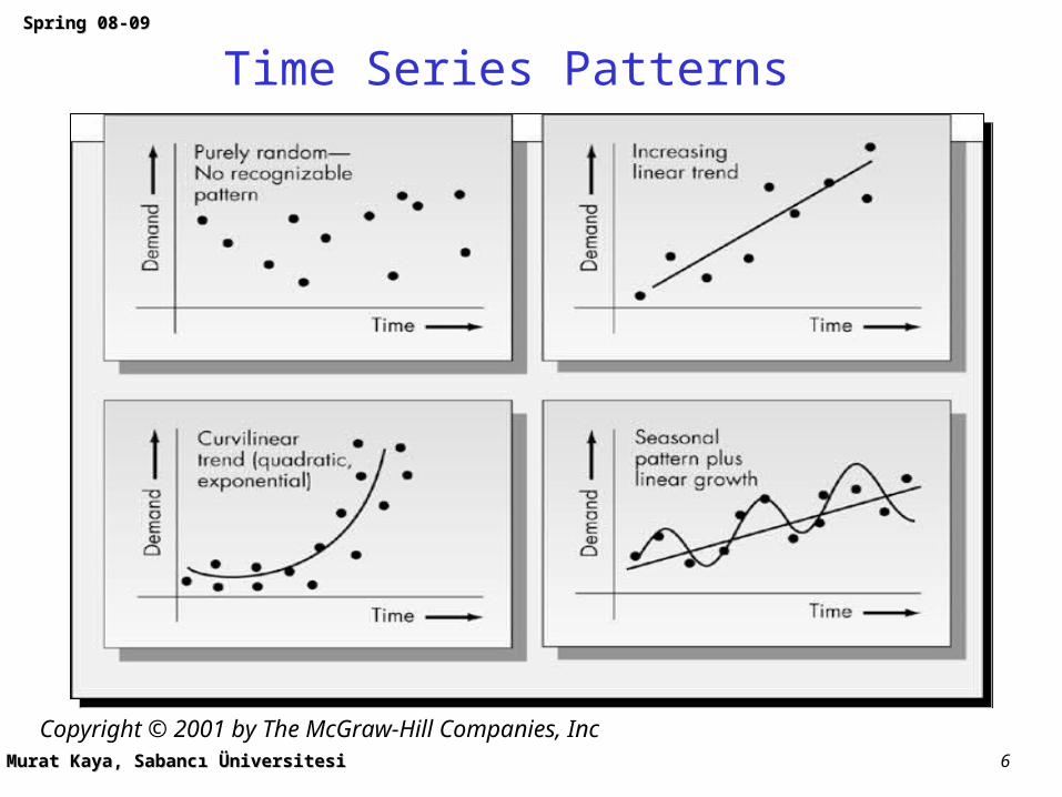
• Patterns in time series– trend: tendency of a time series to exhibit a stable pattern of

growth or decline

– seasonality: having a pattern that repeats in fixed intervals

– cycles: similar to seasonality, but the length and the magnitude of the cycle may vary

– randomness: when there is no recognizable pattern to the data



6

Time Series Patterns

Copyright © 2001 by The McGraw-Hill Companies, Inc



7

Evaluating Forecasts

1 periodin periodfor madeforecast :

demand of valuesobserved ...,...,,,, 321

t-tF

DDDD

t

t

ttt DFe :errorForecast

1001

1

1

AccuracyForecast of Measures

1

1

2

1

n

i i

i

n

ii

n

ii

D

e

nMAPE

en

MSE

en

MAD



8

Random versus Biased Forecast Errors




9

Forecasting Stationary Time Series

ttD

• Stationary time series: Each observation can be represented by a constant plus a random fluctuation

•

• Two methods– moving averages (MA)

– exponential smoothing (ES)



10

Moving Averages (MA)

Nttt

t

Ntiit DDD

ND

NF

...

1121

1

Ntttt DDN

FF

11

• A moving average of order N is the arithmetic average of the most recent N observations

• When calculating the forecast for the following period (period t+1), we do not need to recalculate the N-period average because

• Example 2.2



11

Moving Average Lags Behind the Trend



12

Exponential Smoothing (ES)

1 2 2

2

1 2 2

Substituting 1 we obtain

1 1

t t t

t t t t

F D F

F D D F

11 1 ttt FDF

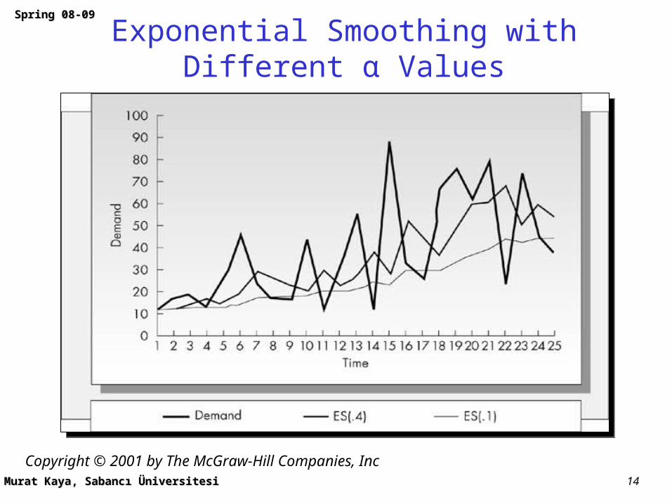
• The current forecast is the weighted average of the current observation of demand and the last forecast

• High α: forecast reacts better, however it is less stable–

011

get we way,in this Continuing

iit

it DF



13

Weights in Exponential Smoothing




14

Exponential Smoothing with Different α Values




15

Example 2.3 from Nahmias

2001 112 FDF

• Observed number of failures:– 200, 250, 175, 186, 225, 285, 305 190

• Assume F1 was 200 (we need a starting value)

• Using α=0.1

The forecasts are quite stable due to

low α



16

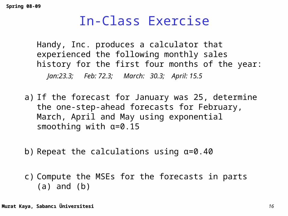
In-Class Exercise

Handy, Inc. produces a calculator that experienced the following monthly sales history for the first four months of the year:

Jan:23.3; Feb: 72.3; March: 30.3; April: 15.5

a) If the forecast for January was 25, determine the one-step-ahead forecasts for February, March, April and May using exponential smoothing with α=0.15

b) Repeat the calculations using α=0.40

c) Compute the MSEs for the forecasts in parts (a) and (b)



17

Solution - 1

Ft = Dt-1 + (1-)Ft-1



18

Solution - 2



19

Similarities Between Moving Averages and Exponential Smoothing

• Stationary demand assumption– can also handle shifts in demand (will adjust)

• Single parameter: N, α– small N or large α results in

• greater weight on current data

• more responsive forecasts

• Not effective in catching trends– both lag behind trends



20

Differences Between Moving Averages and Exponential Smoothing

• – ES assigns weight to all past data points

– MA uses only the latest N

• – ES requires only the latest data point

– MA requires to save N past data points



21

Forecasting Time Series with Trend

• Two methods

– regression analysis (we will not cover)• fits a straight line to a set of data

– double exponential smoothing (Holt’s method)• simultaneous smoothing on the series and the trend



22

Double Exponential Smoothing Using Holt’s Method

11

11

1

1

tttt

tttt

GSSG

GSDS

tttt GSF ,

InterceptSlope

: tperiodin madeforecast ahead-step- τThe

• Initialization issue: The best way is to use some initial period data to estimate the initial intercept (S0) and slope (G0)



23

Example 2.5 from Nahmias• Observed number of failures: 200, 250, 175, 186, 225, 285, 305, 190

• Assume S0 = 200, G0 = 10. Use α=0.1, β=0.1

t Ft-1,t (forecasted) Dt (actual) St (intercept) Gt (slope)

0 --- --- 200.0 10.0

1 210.0 200 209.0 9.9

2 218.9 250 222.0 10.2

3 232.2 175 226.5 9.6

4 236.1 186 … …

5 240.3 225 … …

6 247.7 285 … …

• Multi-step ahead forecast: F2,5=S2+(3)G2=222+(3)(10.2)=252.6



24

Forecasting Seasonal Series

• A seasonal series is a series that has a pattern repeating

every N periods (length of the season)

• Note that this is different than using “season” to refer to a

time of the year

• To model seasonality, use seasonal factors:

• ct represents the average amount that the demand in the tth

period of the season is above or below the overall average

• We will study the Winter’s method

– triple exponential smoothing

Ncccc tN where,...,, 21



25

Winter’s Method: Seasonal Series with Increasing Trend




26

Winter’s Method

• Assume a model of the form

Ntt

tt

tttt

ttNt

tt

cS

Dc

GSSG

GSc

DS

1

1

1

11

11

Nttttt cGSF ,

tttt cGD

Trend

Seasonal factors



27

Winter’s Method: Initialization Procedure

• Check Nahmias, page 85 for details

• Use at least two seasons of data (2N data)

• Calculate the sample means for the two seasons V1, V2

• Calculate the initial slope estimate G0

–

• Calculate the initial intercept estimate S0

–

• Calculate the initial seasonal factors–

– find the average of each seasonal factor

– normalize the seasonal factors (so that they sum up to 1)



28

Example 2.8 from Nahmias

• The data set: 10, 20, 26, 17, 12, 23, 30, 22

• Initialize

• Suppose that at time t=1, we observe D1=16. Update the

equations using α=0.2, β=0.1, γ=0.1

• Suppose that we observe one full year of demand given by D1=16, D2=33, D3=34, D4=26. Update the equations again

Season 1 Season 2



29

Seasonal Demand, No Trend




30

Affecting the Demand

• “The best way to forecast the future is to create it”

Peter Drucker

• “Forecasting the demand” versus “demand planning”, or “demand management”

• Firms can “affect” their demand through their actions– promotions

– sales effort

• Encourages the retailers / wholesalers to “forward buy”

• What are the effects of past promotions in the health of forecasting data?



31

Some Practical Issues

• Sales data versus demand data– how can a firm capture “lost sales” ?

• Forecasting demand for a new product is difficult– will it generate demand, or will it steal demand from existing

products?

• Forecasting assumes that history represents future. What if there are some external changes?– a new competitor

• Slow-moving items are hard to forecast– sparse data

murat kaya, sabancı Üniversitesi spring 08-09 1 ms 401 - production and service systems operations...

Documents

sabanc niversitesi spring

forecasts forecast

trend slide

data slide

time series trend

current forecast

time series patterns

past history slide