mutant: balancing storage cost and latency in lsm-tree data...
TRANSCRIPT

Mutant: Balancing Storage Cost and Latency in LSM-Tree DataStores
Hobin YoonGeorgia Institute of Technology
Juncheng YangEmory University
Sveinn Fannar KristjanssonSpotify
Steinn E. SigurdarsonTakumi
Ymir VigfussonEmory University
& Reykjavik [email protected]
Ada GavrilovskaGeorgia Institute of Technology
ABSTRACTToday’s cloud database systems are not designed for seamless cost-performance trade-offs for changing SLOs. Database engineers havea limited number of trade-offs due to the limited storage types of-fered by cloud vendors, and switching to a different storage typerequires a time-consuming data migration to a new database. Wepropose Mutant, a new storage layer for log-structured mergetree (LSM-tree) data stores that dynamically balances databasecost and performance by organizing SSTables (files that store asubset of records) into different storage types based on SSTable ac-cess frequencies. We implemented Mutant by extending RocksDBand found in our evaluation thatMutant delivers seamless cost-performance trade-offs with the YCSB workload and a real-worldworkload trace. Moreover, through additional optimizations,Mu-tant lowers the user-perceived latency significantly comparedwith the unmodified database.
CCS CONCEPTS• Information systems → Record and block layout; DBMSengine architectures; Cloud based storage; Hierarchical storagemanagement; • Theory of computation → Data structures and
algorithms for data management;
KEYWORDSLSM-tree data stores, Database storage systems, Cloud databasesystems, and Seamless cost and latency trade-offs
ACM Reference Format:Hobin Yoon, Juncheng Yang, Sveinn Fannar Kristjansson, Steinn E. Sigur-darson, Ymir Vigfusson, and Ada Gavrilovska. 2018. Mutant: BalancingStorage Cost and Latency in LSM-Tree Data Stores. In SoCC ’18: ACM Sym-
posium on Cloud Computing, October 11–13, 2018, Carlsbad, CA, USA. ACM,New York, NY, USA, 12 pages. https://doi.org/10.1145/3267809.3267846
Permission to make digital or hard copies of all or part of this work for personal orclassroom use is granted without fee provided that copies are not made or distributedfor profit or commercial advantage and that copies bear this notice and the full citationon the first page. Copyrights for components of this work owned by others than ACMmust be honored. Abstracting with credit is permitted. To copy otherwise, or republish,to post on servers or to redistribute to lists, requires prior specific permission and/or afee. Request permissions from [email protected] ’18, October 11–13, 2018, Carlsbad, CA, USA
© 2018 Association for Computing Machinery.ACM ISBN 978-1-4503-6011-1/18/10. . . $15.00https://doi.org/10.1145/3267809.3267846
Cost($/
year)
Latency(ms)
300M30M
0.1
1.5
Fast DB
MUTANTMUTANT-OPT
Slow DB
Figure 1: Mutant provides seamless cost-performance trade-offs between “fast database” and “slow database”, and better cost-
performance trade-offs with an extra optimization.
1 INTRODUCTIONThe growing volume of data processed by today’s global web ser-vices and applications, normally hosted on cloud platforms, hasmade cost effectiveness a primary design goal for the underlyingdatabases. For example, if the 100,000-node Cassandra clusters Ap-ple uses to fuel their services were instead hosted on AWS (AmazonWeb Services), then the annual operational costs would exceed$370M1. Companies, however, also wish to minimize their databaselatencies since high user-perceived response times of websites loseusers [28] and decrease revenue [26]. Since magnetic storage is acommon latency bottleneck, cloud vendors offer premium storagemedia like enterprise-grade SSDs [8, 30] and NVMe SSDs [15]. Yeteven with optimizations on such drives, like limiting power usage[11, 17] or expanding the encoding density [31, 38], the price oflower-latency storage media can eat up the lion’s share of the totalcost of operating a database in the cloud (Figure 2).
Trading off database cost and latency involves tedious and error-prone effort for operators. Consider, for instance, the challengesfaced by an engineer intending to transition a large database systemoperating in the cloud to meet a budget cut. When the databasesystem accommodates only one form of storage medium at a time,they must identify a cheaper media – normally a limited set ofoptions – while minimizing the ensuing latencies. They then live-migrate data to the new database and ultimately all customer-facing1Conservatively calculated using the price of AWS EC2 c3.2xlarge instance, of whichstorage size adequately hosts the clusters’ data.

SoCC ’18, October 11–13, 2018, Carlsbad, CA, USA H. Yoon et al.
Cost
(K
$ /
year)
CPU +Memory
Storage
EBSMagCold
EBSMag
EBSSSD
LocalSSD
02468
10121416
Figure 2: Fast storage is costly. Cost to host an IaaS database in-
stance for 1 year using various storage devices. Storage cost can be
more than 2× the cost of CPU and memory. Based on the pricing of
EC2 i2.2xlarge instance (I/O-optimized with 1.6 TiB storage device)
[8].
applications, a process that can take months as in the case of Net-flix [9]. Every subsequent change in the budget, including possibleside-effects from the subsequent change in latencies, undergoes asimilar laborious process. In the rare cases where the database doessupport multiple storage media, such as the round-robin strategyin Cassandra [3] or per-level storage mapping in RocksDB [6], theengineer is stuck with either a static configuration and a suboptimalcost-performance trade-off, or they must undertake cumbersomemanual partitioning of data and yet still be limited in their costoptions to accommodate budget restrictions.
We argue that cloud databases should support seamless cost-performance trade-offs that are aware of budgets, avoiding the needto manually migrate data to a new database configuration whenworkloads or cost objectives change. Here, we present Mutant:a layer for log-structured merge tree (LSM-tree) data stores [21,33] that automatically maintains a cost budget while minimizinglatency by dynamically keeping frequently-accessed records onfast storage and less-frequently-accessed data on cheaper storage.Rather than the trade-off between cost-performance points beingzero-sum, we find that by further optimizing the placement ofmetadata,Mutant enables the data store to simultaneously achieveboth low cost and low latency (Figure 1).
The key insight behind Mutant is to exploit three propertiesof today’s data stores. First, the access patterns in modern work-loads exhibit strong temporal locality, and the popularity of objectsfades over time [14, 24]. Second, LSM-tree designs imply that datathat arrives in succession is grouped into the same SSTable, beingsplit off when full. Because of the access patterns, the frequencyof which an SSTable is accessed decreases with the SSTable’s age.Third, each SSTable of which the database is comprised is a portableunit, allowing them to be readily migrated between various cloudstorage media. Mutant combines these properties and continu-ously migrates older SSTables and, thus, colder data to slower andcheaper storage devices.
Dynamically navigating the cost-performance trade-off comeswith challenges. To minimize data access latencies while meet-ing the storage cost SLO (service level objective), the Mutantdesign includes lightweight tracking of access patterns and acomputationally-efficient algorithm to organize SSTables by theiraccess frequencies. Migrations of SSTables are not free, soMutant
also contains a mechanism to minimize rate of SSTable migrationswhen SSTable access frequencies are in flux.
We implementMutant by modifying RocksDB, a popular, high-performance LSM tree-based key-value store [7]. We evaluatedour implementation on a trace from the backend database ofa real-world application (the QuizUp trivia app) and the YCSBbenchmark [18]. We found that Mutant provides seamless cost-performance trade-off, allowing fine-grained decision making ondatabase cost through an SLO. We also found that with our furtheroptimizations, Mutant reduced the data access latencies by up to36.8% at the same cost compared to an unmodified database.
Our paper makes the following contributions:• We demonstrate that the locality of record references in real-world workloads corresponds with the locality of SSTable refer-ences: there is a high disparity in SSTable access frequencies.
• We design an LSM tree database storage layer that provides seam-less cost-performance trade-offs by organizing SSTables withan algorithm that has minimal computation and IO overheadsusing SSTable temperature, an SSTable access popularity metricrobust from noise.• We further improve the cost-performance trade-offs with op-timizations such as SSTable component organization, a tightintegration of SSTable compactions and migrations, and SSTablemigration resistance.• We implement Mutant by extending RocksDB, evaluate with asynthetic microbenchmarking tool and a real-world workloadtrace, and demonstrate that (a) Mutant provides seamless cost-performance trade-offs and (b)Mutant-opt, an optimized ver-sion of Mutant, reduces latency significantly over RocksDB.
2 BACKGROUND AND MOTIVATIONThe SSTables and SSTable components of LSM-tree databases havesignificant data access disparity. Here, we will argue that this im-balance is created from locality in workloads, and gives us an op-portunity to separate out hotter and colder data at an SSTable levelto store on different storage media.
2.1 Preliminaries: LSM-Tree DatabasesOur target non-relational databases (BigTable, HBase, Cassandra,LevelDB and RocksDB), all popular for modern web services fortheir reputed scalability and high write throughput, all share acommon data structure for storage: the log-structured merge (LSM)tree [1, 7, 16, 21, 25].We start with a brief overview of how LSM tree-based storage is organized, in particular the core operations (andnamesake) of log-structured writes and merge-style reads, deferringfurther details to the literature [33].
Writes: When a record is written to an LSM-tree database, it isfirst written to the commit log for durability, and then written tothe MemTable, an in-memory balanced tree. When the MemTablebecomes full from the record insertions, the records are flushedto a new SSTable. SSTable contains a list of records ordered bytheir keys: the term SSTable originates from sorted-string table.The batch writing of records is the key design for achieving highwrite throughputs by transforming random disk IOs to sequentialIOs. A record modification is made by appending a new version to

Mutant: Balancing Storage Cost and Latency in LSM-Tree Data Stores SoCC ’18, October 11–13, 2018, Carlsbad, CA, USAR
ead
fre
q.
(rela
tive)
Object age (day)
1-min avg1-hour avg
10-710-610-510-410-310-210-1
1
0 2 4 6 8 10 12 14 1610-4
10-3
10-2
10-1
1
0 10 20 30 40 50
Acc
ess
fre
quency
Access frequency rank
SSTa
ble
s
Time (day)
10-3
10-2
10-1
1
0 2 4 6 8 10 12 14 Accessfreq.
Figure 3: Record age and its accessfrequency from the QuizUp data access
trace. Access frequencies are aggregated
over all records and normalized.
Figure 4: SSTable access frequencydistribution on day 15 of the 16-day
QuizUp trace replay.
Figure 5: SSTable access frequencies over time. Eachrectangle represents an SSTable with a color representing
its access frequency. SSTable heights at the same time are
drawn proportionally to their sizes.
the database, and a record deletion is made by appending a specialdeletion marker, tombstone.
Reads:When a record is read, the database consults the MemTableand the SSTables that can possibly contain the record, merges allmatched records, and then returns the merged result to the client.
Leveled compaction: The merge-style record read implies thatread performance will depend on the number of SSTables that needto be opened, the number of which is called a read amplification fac-tor. To reduce the read amplification, the database reorganizes SSTa-bles in the background through a process called SSTable compaction.In this work, we focus on the leveled compaction strategy [33] thatwas made popular by LevelDB, and has been adopted by Cassandraand RocksDB [7, 19].
The basic version of leveled compaction decreases read ampli-fication by imposing two rules to organize SSTables into a hierar-chy. First, SSTables at the same level are responsible for disjointkeyspace ranges, which guarantees a read operation to read at most-one SSTable per level2. Second, the number of SSTables at eachlevel increases exponentially from the previous level, normally bya factor of 10. Thus, a read operation in a database consisting of NSSTables only needs to look up O (logN ) SSTables [6, 19, 21, 27].
2.2 Locality in Web WorkloadsModern web workloads have repeatedly been shown to have hightemporal data access locality: access frequency drops off quicklywith age [14, 24, 37]. We observe that a similar temporal localityexists with database records from the analysis of a real-world data-base access trace: we gathered a 16 day trace of the key-value storesunderlying Plain Vanilla’s QuizUp trivia app while serving tensof millions of players [5]. Figure 3 shows a sharp drop of recordaccesses as records become old.
2.3 Locality in SSTable AccessesThe locality in record accesses, combined with the batch writing ofrecords to SSTables, leads to the locality in SSTable accesses. Weconfirm the SSTable access frequency disparity by analyzing the
2Level-0 SSTables are exceptions to the rule, however, databases limit those SSTablesto a small number.
SSTable accesses using the QuizUp workload. First, at a given time,only a small number of SSTables are frequently accessed and theothers are minimally accessed: the difference between the most andthe least frequently accessed ones is as big as 4 orders of magnitudes(see Figure 4). Second, the access disparity persists throughout thetime, as shown by the time vs. SSTable accesses in Figure 5. Asmore records are inserted over time, the number of infrequentlyaccessed SSTables (“cold” SSTables) increases, while the numberof frequently accessed SSTables (“hot” SSTables) stays about thesame.
2.4 Locality in SSTable Component AccessesNot only do SSTables have different access frequencies, but alsoSSTable components have different access frequencies. In this sub-section, we analyze how frequently each of the SSTable componentsare accessed. An SSTable consists of metadata and database records,and metadata includes a Bloom filter and a record index, both ofwhich reduce the read IOs: Bloom filter [13] is for quickly skippingan SSTable when the record doesn’t exist in it, and record index isfor efficiently locating record offsets.
Component Access Frequencies: To read a record, the databasemakes a sequence of SSTable component accesses: First, the data-base checks the keyspace range of the SSTables at each level to findthe SSTables that may contain the record. There is at most 1 suchSSTable per level thanks to the leveled organization of SSTables(§2.1); in other words, there are at most N SSTables, where N is thenumber of levels. Second, for each SSTable that passes the keyspacerange test, the database checks the Bloom filter to see if the recordis in the SSTable or not. Out of the N SSTables, there is only 1SSTable that contains the record and N − 1 SSTables that do not.In the former SSTable, the Bloom filter always answers maybe
3, inthe latter SSTables, the Bloom filter answers maybe with a falsepositive ratio f p. Thus, on average, 1 + (N − 1) · f p read requestsgo to the next step. The number becomes approximately 1 whenf p is very small such as 0.01, which is the case with most of thedatabases. Third, using the record index, the database locates andreads the record.3Bloom filter tests if an item is in a set or not, and answers a definitely no or a maybe
with a small false positive ratio.
SoCC ’18, October 11–13, 2018, Carlsbad, CA, USA H. Yoon et al.
File names(simplified) Type
Access frequency(relative toBloom filter)
Size Accessfrequency
/ sizeBytes %
Filter.db Bloom filter 1 149,848 0.11 869
Summary.db Index (top)≈
1N
15,056 0.01 60/NIndex.db Index (bottom) 2,152,386 1.62Data.db Records 130,219,353 98.24 1/N
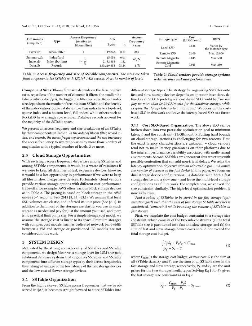
Table 1: Access frequency and size of SSTable components. The sizes are takenfrom a representative SSTable with 127,167 1-KB records. N is the number of levels.
Storage type Cost IOPS($/GB/month)
Local SSD 0.528 Varies bythe instance type
Remote SSD 0.100 Max 10,000Remote Magnetic 0.045 Max 500Remote Magnetic 0.025 Max 250Cold
Table 2: Cloud vendors provide storage optionswith various cost and performance.
Component Sizes: Bloom filter size depends on the false positiveratio, regardless of the number of elements it filters: the smaller thefalse positive ratio f p is, the bigger the filter becomes. Record indexsize depends on the number of records in an SSTable and the densityof the index entries. Some databases like Cassandra have a top-level,sparse index and a bottom-level, full index, while others such asRocksDB have a single sparse index. Database records account forthe majority of the SSTable space.
We present an access frequency and size breakdown of an SSTableby their components in Table 1. In the order of Bloom filter, record in-
dex, and records, the access frequency decreases and the size increases:
the access frequency to size ratio varies by more than 3 orders ofmagnitudes with a typical number of levels, 3 or more.
2.5 Cloud Storage OpportunitiesWith such high access frequency disparities among SSTables andamong SSTable components, it would be a waste of resources ifwe were to keep all data files in fast, expensive devices; likewise,it would be a lost opportunity in performance if we were to keepall files in slow, inexpensive devices. Fortunately, cloud vendorsprovide various storage options with different cost-performancetrade-offs: for example, AWS offers various block storage devicesas in Table 2. The pricing is based on block storage in the AWSus-east-1 region in Feb. 2018 [8, 36] (§5.1). We assume that localSSD volumes are elastic, and inferred its unit price (See §5.1). Inaddition to that, most of the storages are elastic: you use as muchstorage as needed and pay for just the amount you used, and thereis no practical limit on its size. For a simple storage cost model, weassume the storage cost is linear to its space. Premium storageswith complex cost models, such as dedicated network bandwidthbetween a VM and storage or provisioned I/O models, are notconsidered in this work.
3 SYSTEM DESIGNMotivated by the strong access locality of SSTables and SSTablecomponents, we design Mutant, a storage layer for LSM-tree non-relational database systems that organizes SSTables and SSTablecomponents into different storage types by their access frequencies,thus taking advantage of the low latency of the fast storage devicesand the low cost of slower storage devices.
3.1 SSTable OrganizationFrom the highly skewed SSTable access frequencies that we’ve ob-served in §2.3, it becomes straightforward to store SSTables into
different storage types. The strategy for organizing SSTables ontofast and slow storage devices depends on operator intentions, de-fined as an SLO. A prototypical cost-based SLO could be: “we willpay no more than $0.03/GB/month for the database storage, while
keeping the storage latency to a minimum.” We focus on the cost-based SLO in this work and leave the latency-based SLO as a futurework.
3.1.1 Cost SLO-Based Organization. The above SLO can bebroken down into two parts: the optimization goal (a minimumlatency) and the constraint ($3/GB/month). Putting hard boundson cloud storage latencies is challenging for two reasons. First,the exact latency characteristics are unknown – cloud vendorstend not to make latency guarantees on their platforms due tothe inherent performance variability associated with multi-tenantenvironments. Second, SSTables are concurrent data structures withpossible contention that can add non-trivial delays. We relax thelatency optimization objective into an achievable goal: maximize
the number of accesses to the fast device. In this paper, we focus ondual storage device configurations – a database with both a faststorage device and a slow one – and leave the multi-level storageconfigurations as a future work. For completeness, we convert thesize constraint similarly. The high-level optimization problem isnow as follows:
Find a subset of SSTables to be stored in the fast storage (opti-
mization goal) such that the sum of fast storage SSTable accesses is
maximized, (constraint) while bounding the volume of SSTables in
fast storage.First, we translate the cost budget constraint to a storage size
constraint, which consists of the two sub-constraints: (a) the totalSSTable size is partitioned into fast and slow storage, and (b) thesum of fast and slow storage device costs should not exceed thetotal storage cost budget.
Pf Sf + PsSs ≤ CmaxSf + Ss = S
(1)
where Cmax is the storage cost budget, or max cost, S is the sum ofall SSTable sizes, Sf and Ss are the sum of all SSTable sizes in thefast storage and slow storage, respectively, Pf and Ps are the unitprices for the two storages media types. Solving Eq 1 for Sf givesthe fast storage size constraint as in Eq 2.
Sf <Cmax − PsS
Pf − Ps= Sf ,max (2)

Mutant: Balancing Storage Cost and Latency in LSM-Tree Data Stores SoCC ’18, October 11–13, 2018, Carlsbad, CA, USA
We formulate the general optimization goal as:
maximize∑
i ∈SSTablesAixi
subject to∑
i ∈SSTablesSixi ≤ Sf ,max and xi ∈ {0, 1}
(3)
where Ai is the number of accesses to the SSTable i , Si is the sizeof the SSTable i , and xi represents whether the SSTable i is storedin the fast storage or not.
The resulting optimization problem, Eq 3, is equivalent to a0/1 knapsack problem. In knapsack problems, you are given a setof items that each has a value and a weight, and you want tomaximize the value of the items you can put in your backpackwithout exceeding a fixed a weight capacity. In our problem setting,the value and weight of an item correspond to the size and accessfrequency of an SSTable; the backpack’s weight capacity matchesthe maximum fast storage device size, Sf ,max.
3.1.2 Greedy SSTable Organization. The 0/1 knapsack prob-lem is a well-known NP-hard problem and often solved with adynamic programming technique to give a fully polynomial timeapproximation scheme (FPTAS) for the problem. However, thisapproach for organizing SSTables has two complications.
First, the computational complexity of the dynamic programming-based algorithm is impractical: it takes bothO (nW ) time andO (nW )space, where n is the number of SSTables andW is the number ofdifferent sub-capacities to consider. To illustrate the scale, a 1 TiBdisk using 64 MiB SSTables will contain 10,000s of SSTables andhave 1012 sub-capacities to consider since SSTable sizes can varyat the level of bytes. Moreover, this O (nW ) time complexity wouldbe incurred every epoch during which SSTables are reorganized.
Second, optimally organizing SSTables at each organizationepoch can cause frequent back-and-forth SSTable migrations. Sup-pose you have a cost SLO of $3/record and the database usestwo storage devices, a fast and a slow storage that cost $5/recordand $1/record, respectively. Initially, the average cost/record is2.71 = 5×3+1×(2+2)
3+2+2 , with the maximum amount of SSTables inthe fast storage while satisfying the cost SLO (Figure 6a at timet1). When a new SSTable D is added, it most likely contains themost popular items and is placed on the leftmost side (Figure 6aat time t2). We assume that the existing SSTables cool down (asseen in §3.1.3), and their relative temperature ordering remainsthe same. This results in $3.40/record, temporarily violating thecost SLO; however, at the next SSTable organization epoch, theSSTables are organized with an optimal knapsack solution, bring-ing the cost down to $3.00/record (Figure 6a at time t2′). Similarly,when another SSTable E is added, the SLO is temporarily violated,but observed soon after (Figure 6a at time t3 and t3′). During theorganizations, SSTable B migrates back-and-forth between storagetypes, a maneuver that is harmful to read latencies: the latenciescan temporarily spike by more than an order of magnitude.
To overcome these challenges, we use a simple greedy 2-approximation algorithm. Here, items are ordered by decreasingratio of value to weight, and then put in the backpack one at a timeuntil no more items fit. In our problem setting, an item’s value toweight ratio corresponds to an SSTable’s access frequency dividedby its size, which is captured by SSTable temperature (defined in
§3.1.3). The computational complexity of the greedy algorithms isO (n logn) withO (n) space instead ofO (nW ) for both with dynamicprogramming. The log-factor in the time stems from the need tokeep SSTable references sorted in-place by temperature. However,the instantaneous worst-case access latency of the SSTables chosento put into fast versus cold storage can be twice that of the dynamicprogramming algorithm [23], although we rarely see worst-casebehavior exhibited in practice. The algorithmic trade-off thus liesbetween reducing computational complexity versus minimizingSSTable accesses latency.
3.1.3 SSTable Temperature. So far, we have discussed optimalchoices moment-to-moment, but access latencies are dynamicalquantities that depend on the workload.Mutantmonitors SSTableaccesses with an atomic counter for each SSTable. However, naïvelyusing the counters for prioritizing popular tables has two prob-lems:• Variable SSTable sizes: The size of SSTables can differ fromthe configured maximum size (64 MiB in RocksDB and 160 MiBin Cassandra). Smaller SSTables are created at the compactionboundaries where the SSTables are almost always not full. BiggerSSTables are created at L0, where SSTables are compacted toeach other with a compaction strategy different from leveledcompaction such as size-tiered compaction.• Fluctuations of the observed access frequency: The coun-ters can easily be swayed by temporary access spikes and dips:for example, an SSTable can be frequently accessed during aburst and then cease to receive any accesses, a problem arisingwhen a client has a networking issue, or a higher-layer cacheeffectively gets flushed due to code changes, faults or mainte-nance. Such temporary fluctuations could cause SSTables to befrequency reorganized.
To resolve these issues, we smooth the access frequencies throughan exponential average. Specifically, the SSTable temperature isdefined as the access frequencies in the past epoch divided by theSSTable size with an exponential decay applied 4: the sum of thenumber of accesses per unit size in the current time window andthe cooled-down temperature of the previous time window. Naïveapplication of exponential averages would start temperatures at 0,which interferes with the observation that SSTables start out hot.Instead, we set the initial temperature in a manner consistent withthe initial SSTable access frequency as follows:
Tt =
(1 − α ) ·A(t−1,t ]
S+ α ·Tt−1, if t > 1
A(0,1]S, if t = 1
(4)
where Tt is the temperatures at time t , A(t−1,t ] is the number ofaccesses to the SSTable during the time interval (t − 1, t], S is theSSTable size, and α is a cooling coefficient in the range of (0, 1].
3.2 SSTable Component OrganizationWe have thus far discussed how Mutant organizes SSTables them-selves by their access frequencies. We discovered that Mutantcan further benefit by considering the components of SSTables in
4It was inspired by Newton’s law of cooling [12].

SoCC ’18, October 11–13, 2018, Carlsbad, CA, USA H. Yoon et al.
2.71
3.40
$/Record
3.00
3.33
2.66
SSTables ordered by temperature (hot to cold)
Time
t1
t2
t2’
t3
t3’
SSTable migration
SSTable in fast storage
SSTable in slow storage
ABC
D C B A
D C B A
D C B AE
D C B AE
2.71
3.40
2.20
2.66
SSTables ordered by temperature (hot to cold)
$/Record
ABC
ABCD
ABCD
ABCDE
Time
t1
t2
t2’
t3
t3’
(a) Optimal SSTable organization (b) Greedy organization of SSTables
Figure 6: Greedy SSTable organization reduces SSTable migrations.
the same light. We observed that the SSTable metadata portion,specifically the Bloom filter and record index, have multiple magni-tudes higher access-to-size ratios than the SSTable records portion(see §2.4). Thus,Mutant will strive to keep the metadata on faststorage devices, going so far as to pinning metadata in memory.The trade-off considered here weighs the reduced access latencyfor metadata because they are always served from memory to thereduced file system cache hit ratio for SSTable records due to thereduced memory available for the file system cache.
The organization of SSTable components depends on the phys-ical layout of an SSTable. On one hand, in databases that storeSSTable components in separate files (e.g., Cassandra), Mutantstores themetadata files in a configured storage device such as a fast,expensive one. On the other hand, in databases that store SSTablecomponents all in a single file (e.g., RocksDB), Mutant choosesnot to separate out the metadata and records. The latter optimiza-tion would involve both implementing a transactional guaranteebetween the metadata and records, and then rewriting the storageengine and tools. Instead,Mutant keeps the SSTable metadata inmemory once it is read. We note that some LSM-tree databasesalready cache metadata, but only partially: RocksDB provides anoption to keep only the L0 SSTable metadata in memory.
4 IMPLEMENTATIONWe implemented Mutant by modifying RocksDB, a high-performance key-value store that was forked from LevelDB [7].The core of Mutant was implemented in C++ with 658 lines ofcode, and 110 lines of code were used to integrate Mutant withthe database.
4.1 Mutant APIMutant communicates with the database via minimal API consist-ing of three parts:
Initialization: A database client initializesMutantwith a storageconfiguration: for example, a local SSD with $0.528/GB/month andan EBSmagnetic diskwith $0.045/GB/month (Listing 1). The storagedevices are specified from fast to slow with the (path, unit cost)pairs. A client sets or updates a target cost with SetCost().
SSTable Temperature Monitoring: The database then registersSSTables as they are created with Register(), unregisters them as
Options opt;opt.storages.Add("/mnt/local−ssd1/mu−rocks−stg", 0.528,"/mnt/ebs−st1/mu−rocks−stg", 0.045);
DB::Open(opt);DB::SetCost(0.2);
Listing 1: Database initialization with storage options
// Initializationvoid Open(Options);void SetCost(target_cost);// SSTable temperature monitorvoid Register(sstable);void Unregister(sstable);void Accessed(sstable);// SSTable organizationvoid SchedMigr();sstable PickSstToMigr();sstable GetTargetDev();
Listing 2: Mutant API
they are deleted with Unregister(), and calls Accessed() so thatMutant can monitor the SSTable accesses.
SSTable Organization: SSTable Organizer triggers an SSTablemigration when it detects an SLO violation or finds a better or-ganization by scheduling a migration with SchedMigr(). SSTableMigrator then queries for an SSTable to migrate and to whichstorage device to migrate the SSTable with PickSstToMigr() andGetTargetDev(). GetTargetDev() is also called by SSTable com-pactor for the compaction-migration integration we discuss in§4.3.1.The API and the interactions among Mutant, the database, andthe client are summarized in Listing 2 and Figure 7.
4.2 SSTable OrganizerSSTable Organizer (a) updates the SSTable temperatures by fetch-
and-reset-ting the SSTable read counters and (b) organizes SSTableswith the temperatures and the target cost by solving the SSTableplacement knapsack problem. SSTable Organizer runs the organiza-tion task every organization epoch such as every second. When an

Mutant: Balancing Storage Cost and Latency in LSM-Tree Data Stores SoCC ’18, October 11–13, 2018, Carlsbad, CA, USA
Init()
SetCost()
Un/register()
Accessed()
GetTargetDev()
PickSstToMigr()
SSTable created/deleted
SSTable read
Open database
Set/update target cost
SSTableOrganizer
SSTablecompactor
Base Database MUTANTClient
Open()Configure storages
SSTablemigrator
Comp/migration scheduler
SchedMigr()
Figure 7: Interactions among the client, the database, andMu-tant. Mutant API is depicted in red. Parameters and return values
are omitted for brevity.
SSTable migration is needed, SSTable Organizer asks the databasefor scheduling a migration. Its interaction with the database andthe client is summarized in Figure 8. The two key data structuresused are:
SSTable Access Counter: Each SSTable contains an atomicSSTable access counter that keeps track of the number of accesses.
SSTable-Temperature Map: Each SSTable is associated with atemperature object that consists of the current temperature andthe last update time. The SSTable-Temperature map is concurrentlyaccessed by various database threads as well as SSTable Organizeritself. To provide maximum concurrency,Mutant protects the mapwith a two-level locking: (a) a bottom-level lock for frequent readingand updating SSTable temperature values and (b) a top-level lockfor far less-frequent adding and removing the SSTable referencesto and from the map.SSTable Organizer is concurrently accessed by a number of databasethreads including:
SSTable Flush Job Thread: registers a newly-flushed SSTablewithMutant so that its temperature is being monitored.
SSTable Compaction Job Thread: queries Mutant for the tar-get storage device of the compaction output SSTables. Similar towhat the SSTable flush job does, the newly-created SSTables areregistered with Mutant.
SSTable Loader Thread: registers an SSTable withMutant, whenit opens an existing SSTable.
SSTable Reader Thread: increments an SSTable access counter.
4.3 Optimizations4.3.1 Compaction-Migration Integration. SSTable compactionand SSTable migration are orthogonal events: the former is trig-gered by the leveled SSTable organization and the latter is triggeredby the SSTable temperature change. However, SSTable compactionscause SSTable temperature changes: when SSTables are compacted
SSTablecompactor
Database MUTANT
SSTablemigrator
Update temp
Migr/compscheduler
Storage characteristics
Target cost
Schedulemigration
SSTables
SSTable Organizer
Accessed
Client
Figure 8: SSTable Organizer and its interactions with theclient and the database.
together, their records are redistributed among output SSTablesby their hashed key order, resulting in similar access frequenciesamong output SSTables. Consequently, executing SSTable com-pactions and migrations separately would have caused an ineffi-ciency, the double SSTable write problem. Imagine an SSTable in thefast storage is compacted with two SSTables in the slow storage,creating a new SSTable Ta in the fast storage and two new SSTa-bles Tb and Tc in the slow storage. Because their temperatures areaveraged due to the record redistribution, Ta ’s temperature will below enough to trigger a migration, moving Ta to the slow storage.
Thus,Mutant piggybacks SSTablemigrations with SSTable com-pactions, which we call compaction-migration, effectively reducingthe number of SSTable writes, which is beneficial for keeping thedatabase latency low. Note that either an SSTable compaction oran SSTable migration can take place independently: SSTables canbe compacted without being moved to a different storage device(pure compaction), and an SSTable can be migrated by itself whenSSTable Organizer detects an SSTable temperature change acrossthe organization boundary (single SSTable migration). We analyzehow much SSTable migrations can be piggybacked in §5.4.3.
SSTable flushes, although similar to SSTable compactions, arenot combined with SSTable migrations. Since the newly flushedSSTables are the most frequently accessed (recall §2.3), Mutant al-ways writes the newly flushed SSTables to the fast device, obviatingthe need to combine SSTable flushes and SSTable migrations.
4.3.2 SSTable Migration Resistance. The greedy SSTable or-ganization (§3.1.2) reduces the amount of SSTable churns, the back-and-forth SSTable migrations near the organization temperatureboundary. However, depending on the workload, SSTable churnscan still exist: SSTable temperatures are constantly changing, andeven a slight change of an SSTable temperature can change thetemperature ordering. To further reduce the SSTable churns,Mu-tant defines SSTable migration resistance, a value that representsthe number of SSTables that don’t get migrated when their tem-peratures change. The resistance is tunable by clients and providesa trade-off between the amount of SSTables migrated and howadaptive Mutant is to the changing SSTable temperatures, which

SoCC ’18, October 11–13, 2018, Carlsbad, CA, USA H. Yoon et al.
0.0
0.2
0.4
0.6
0.8
1.0
0.01 0.1 1 10 100
CD
F
Latency (ms)
LocalSSD
EBSMag
(a) 4 KB random read latency
0.0
0.2
0.4
0.6
0.8
1.0
0 100 200 300
CD
FThroughput (MB/sec)
EBSMag
LocalSSD
(b) 64 MB write throughput
Figure 9: Performance of the storage devices, local SSD andEBS magnetic volumes. File system cache was suppressed with di-
rect IO.
affects how wellMutantmeets the target storage cost. We analyzethe trade-off in §5.4.2.
5 EVALUATIONThis section evaluatesMutant by answering the following ques-tions:• How well doesMutantmeet a target cost and adapt to a changein cost? (§5.2.1)• What are the cost-performance trade-offs of Mutant like?(§5.2.2)• Howmuch computation overhead does it take tomonitor SSTabletemperature and calculate SSTable placement? (§5.3)• How much does Mutant benefit from the optimizations includ-ing SSTable component organization? (§5.4)
5.1 Experiment SetupWe used AWS infrastructure for the evaluations. For the virtualmachine instances, we used EC2 r3.2xlarge instances that comewith a local SSD [2]. For fast and slow storage devices, we useda locally-attached SSD volume and a remotely-attached magneticvolume, called EBS st1 type. We measured their small, random readand large, sequential write performances, which are the commonIO patterns for LSM tree databases. Compared to the EBS magneticvolume, local SSD’s read latency was lower bymore than an order ofmagnitude, and its sequential write throughput was higher by 42%(Figure 9). Their prices were $0.528 and $0.045 per GB per month,respectively. Since AWS did not provide a pricing for the local SSD,we inferred the price from the cost difference of the two instancetypes, i2.2xlarge and r3.exlarge, which had the same configurationaside from the storage size [35].
For the evaluation workload, we used (a) YCSB, a workloadgenerator for microbenchmarking databases [18] and (b) a real-world workload trace from QuizUp. The QuizUp workload consistsof 686 M reads and 24 M writes of 2 M user profile records for 16days. Its read:write ratio of 28.58:1 is similar to Facebook’s 30:1 [10].
5.2 Cost-Performance Trade-Offs5.2.1 Cost Adaptability. To evaluate the automatic cost-performance configuration, we vary the target cost while runningMutant and analyze its storage cost and database query latency.
(a)Target cost ($/GB/month)Initial value Changes0.4 0.2 0.3
(b)
Sto
rag
e c
ost
($/G
B/m
onth
)
0
0.1
0.2
0.3
0.4
0.5
(c)
Tota
l S
STa
ble
siz
e(G
B)
0
5
10
In fast storage
In slow storage
(d)
0.01
0.1
1
10
DB
late
ncy
(ms)
Read avg
Read 99th
Write 99thWrite avg
0 1000 2000 3000 4000 5000 6000 7000
00:00 00:15 00:30 00:45 01:00
DB
IO
PS
Time (HH:MM)
Figure 10: Mutant makes cost-performance trade-offs seam-less. Target cost changes over time (a), changes in underlying storage
cost (b), Mutant organizes SSTables to meet the target cost (c) and
the database latencies (d).
We used the YCSB “read latest” workload, which models data accesspatterns of social networks, while varying the target cost: we setthe initial target cost to $0.4/GB/month, lowered it to $0.2/GB/-month, and raised it to $0.3/GB/month, as shown in Figure 10(a).We configured Mutant to update the SSTable temperatures everysecond with the cooling coefficient α = 0.999.
Mutant adapted quickly to the target cost changes with a smallcost error margin, as shown in Figure 10(b). When the target costcame down from $0.4 to $0.2, about 4.5GB of SSTables weremigratedfrom the fast storage to the slow storage at a speed of 55.7 MB/sec;when the target cost went up from $0.2 to $0.3, about 2.5GB ofSSTables were migrated to the other direction at a speed of 34.1MB/sec. The cost error margin depends on the SSTable migrationresistance, a trade-off which we look at in §5.4.2: a 5% SSTablemigration resistance was used in the evaluation. Figure 10(c) showshow Mutant organized the SSTables among the fast and slowstorages to meet the target costs.
Database latency changed asMutant reorganized SSTables tomeet the target costs (Figure 10(d)). Read latency changes werethe expected trade-off as SSTables are reorganized to meet thetarget costs; write latency was rather stable throughput the SSTablereorganizations. The stable write latency is from (a) records arefirst written in MemTable not causing any disk IOs, then batch-written to the disk, minimizing the IO overhead and (b) commit logis always written to the fast storage device regardless of the targetcost. At the start of the experiment, the latency was high and thecost was unstable because the file system cache was empty and theSSTable temperature needed a bit of time to be stabilized. Shortlyafter, the latency dropped and the cost stabilized.

Mutant: Balancing Storage Cost and Latency in LSM-Tree Data Stores SoCC ’18, October 11–13, 2018, Carlsbad, CA, USA
0.1
1
1 10 100
Read late
ncy
(m
s)
Throughput (K IOPS)
Cost
($
/GB
/month
)
0.045
0.1
0.2
0.3
0.4
0.50.528
SlowDB
FastDB
MUTANT
0.01
0.1
1
10
1 10 100
Wri
te late
ncy
(m
s)
Throughput (K IOPS)
Figure 11:Cost-performance trade-off spectrum ofMutant. Read latency (left)and write latency (right) controlling throughput (horizontal axis) by varying the target
cost. Colors and symbols represent storage cost.
0
40
80
120
160
200
240
0 10 20 30 40 50
Read late
ncy
(m
s)
Storage cost (cent)
99%Avg1%
Mutant
EBS Mag
LocalSSD
Figure 12: Cost-latency trade-off with theQuizUp workload trace. Fast and slow databases
are shown in red and blue, respectively. Mutant with
various target costs is shown in purple.
5.2.2 Trade-Off Spectrum. We study the cost-performancetrade-off spectrum by analyzing both database throughput (in IOPS)and latency as the target cost changes. We first set the baselinepoints with two unmodified databases: fast database and slow data-
base, as shown in Figure 11(left). Fast database used a local SSDvolume and had about 12× higher storage cost, 20× higher maxi-mum throughput, and 10× lower read latency than slow database
that used an EBS magnetic volume.The cost-read latency trade-off is shown in Figure 11(left). As
we increased the target cost from the lower bound (slow database’scost) to the upper bound (fast database’s cost), the read latencydecreased proportionally. The throughput-latency curves showsome interesting patterns. First, as you increase the throughput, thelatency increases: fast database. This is because the performancebottleneck was the CPU, and the database saturated when the CPUusage was at 100%. Second, as you increase the throughput, thelatency decreases: slow database. The latency decrease was fromthe batching of the read IO requests at the file system layer. Themaximum throughput was 3 K IO/sec due to the rate limiting ofthe EBS volume [8], rather than the CPU getting saturated. Third,as you increase the throughput, the latency initially decreases andthen increases: Mutant. The latency changes are the combinedeffect of the benefit of IO batching in slow storage and the saturationof CPU.
The write latencies stayed about the same throughout the targetcost changes (Figure 11(right)). The result was as expected, sincethe slow storage is not directly in the write path: records are batch-written to the slow storage asynchronously. Figure 11 confirms thatMutant delivers the cost and maximum throughput trade-off: asthe target cost increased, the maximum throughput increased.
The evaluation with the QuizUp workload again confirms thatMutant delivers a seamless cost-latency trade-off. Similar to withthe YCSB workload, we replayed the QuizUp workload with twobaseline databases andMutant with various cost configurationsas shown in Figure 12.
5.2.3 Comparison with Other SSTable Organizations. Wecompare the cost configurability of Mutant and the other SSTableorganization algorithms, leveled organization and round-robin or-ganization used by RocksDB and Cassandra. RocksDB organizesSSTables by their levels into the storage devices [6]. Starting from
Target cost ($/GB/month)Initial value Changes0.4 0.2 0.3
Sto
rag
e c
ost
($/G
B/m
onth
) 0
0.1
0.2
0.3
0.4
0.5 L: 0 1 2 3 |
L: 0 1 2 | 3
L: 0 1 | 2 3L: 0 | 1 2 3L: | 0 1 2 3
RR
0 1000 2000 3000 4000 5000 6000 7000
00:00 00:15 00:30 00:45 01:00
DB
IO
PS
Time (HH:MM)
Figure 13: Storage cost of Mutant and the other SSTable or-ganization strategies. The blue line (with L) represents RocksDB’s
leveled organization. SSTables at a level before the symbol | go to
the fast storage; SSTables at a level after the symbol go to the slow
storage. The red line (with RR) represents Cassandra’s round-robin
organization, and the black line represents the seamless organization
of Mutant.
level 0 and the first storage device, RocksDB stores all SSTables atcurrent level in the current storage only if all the SSTables can fitin the storage; if the SSTables don’t fit, RocksDB looks at the nextstorage device to see if the SSTables can fit. Cassandra spreads datato storages in a round-robin manner proportional to the availablespace of each of the storages [3].
Figure 13 compares the storage cost of Mutant and the otherSSTable organization algorithms. First, neither of the algorithms isadaptive to the changing target cost. When the target cost changes,your only option is migrating your data to a database with a dif-ferent cost-performance characteristic. Second, leveled SSTableorganization has limited number of configurations. With n SSTablelevels and 2 storage types, SSTables can be split in n + 1 differentways. Thus, even when assuming target cost is to be maintained,there is a limited number of cost-performance options.
5.3 Computational OverheadComputational overhead includes the extra CPU cycles and theamount of memory needed for the SSTable temperature monitoringand SSTable placement calculation. The overhead depends on thenumber of SSTables: the bigger the number of SSTables, the moreCPU and memory are used for monitoring the temperatures and
SoCC ’18, October 11–13, 2018, Carlsbad, CA, USA H. Yoon et al.
(a)
0
20
40
60
80
100
0 1 2 3 4 5 6 7
CPU
(%
)
x+x+x+x+x+x+x+x+x+x+x+x+x+x+x+x+x+x+x+x+x+x+
x+x+x+x+x+x+x+x+x+x+x+x+x+x+x+x+x+x+x+x+x+x+x+x+x+x+x+x+x+
x+x+x+x+x+x+x+x+x+x+x+x+x+x+x+x+x+x+x+x+x+x+x+x+x+x+x+x+x+
x+x+x+x+x+x+x+x+x+x+x+x+x+x+x+x+x+x+x+x+x+x+x+x+x+x+x+x+x+
x+
x+
x+x+x+x+x+x+x+x+x+x+x+x+x+x+x+x+x+x+x+x+x+x+x+x+x+x+x+x+
x+
x+x+x+x+x+x+x+x+x+x+x+x+x+x+x+x+x+x+x+x+x+x+x+x+x+x+x+x
+
x
+
x+x+x+x+x+x+x+x+x+x+x+x+x+x+x+x+x+x+x+x+x+
x+x+x+x+x+x+x+
x+x+
x+x+x+x+x+x+x+x+x+x+x+x+x+x+x+x+x+x+x+x+x+x+x+x+x+x+x+
x+
x
+
x+x+x+x+x+x+x+x+x+x+x+x+x+x+x+x+x+x+x+x+x+x+x+x+x+x+x+x+
x+
x+x+x+x+x+x+x+x+x+x+x+x+x+x+x+x+x+x+x+x+x+x+x+x+x+x+x+x+
x+x+
x+x+x+x+x+x+x+x+x+x+x+x+x+x+x+x+x+x+x+x+x+x+x+x+x+x+x+
x+
x+
x+x+x+x+x+x+x+x+x+x+x+x+x+x+x+x+x+x+x+x+
x+x+x+x+x+x+x+
x+
x+
x+x+x+x+x+x+x+x+x+x+x+x+x+x+x+x+x+x+x+x+x+x+x+x+x+x+x+x+
x+
x+
x+x+x+x+x+x+x+x+x+x+x+x+x+x+x+x+x+x+x+x+x+x+x+x+x+x+x
+
x
+x
+
x+x+x+x+x+x+x+x+x+x+x+x+x+x+x+x+x+x+x+x+x+x+x+x+x+x+x+
x+
x+
x+x+x+x+x+x+x+x+x+x+x+x+x+x+x+x+x+x+x+x+x+x+x+x+x+x+x+
x+
x
+
x
+
x+x+x+x+x+x+x+x
x Unmodified DB+ With computation
1.66% moreCPU
(b)
0.00.51.01.52.0
0 1 2 3 4 5 6 7
Mem
ory
(G
B)
Time (hour)
x+x+x+x+x+x+x+x+x+x+x+x+x+x+x+x+x+x+x+x+x+x+x+x+x+x+x+x+x+x+x+x+x+x+x+x+x+x+x+x+x+x+x+x+
x+x+x+x+x+x+x+x+x+x+x+x+x+x+x+x+x+x+x+x+x+
x+x+x+x+x+x+x+x+x+x+x+x+x+x+x+x+x+x+x+x+x+x+x+x+x+x+x+x+x+x+x+x+x+x+x
+x+x+x+x+x+x+x+x+x+x+x+x+x+x+x+x+x
+x+x+x+x+x+x+x+x+x+x+x+x+x+x+x+x+x+x+x+x+x+x+x+x+x+x+x+x+x+x+x+x+x+x+x+x+x+x+x+x+x+x+x+x+x+x+x+x
+x+x+x+x+x+x+x+x+x+x+x+x+x+x+x+x+x+x+x+x+x+x+x+x+x+x+x+x+x+x+x+x+x+x+x+x+x+x+x+x+x+x+x+x+x
+x+x+x+x+x+x+x+x+x+x+x+x+x+x+x+x+x+x+x+x+x+x+x+x+x+x+x+x+x+x+x+x+x+x+x+x+x+x+x+x+x+x+x+
x+x+x+x+x+x+x+x+x+x+x+x+x+x+x+x+x+x+x+x+x+x+x+x+x+x+x+x+x+x+x+x+x+
x+x+x+x+x+x+x+x+x+x+x+x+x+x+x+x+x+x+x+x+x+x+x+x+x+x+x+x+x+x+x+x+x+x+x+x+x+x+x+x+x+x+x+x+x+x+x+x+x+x+x+x+x+x+x+x+x+x+x+
x+x+x+x+x+x+x+x+x+x+x+x+x+x+x+x+x+x+x+x+x+x+x+x+x+x+x+x+x+x+x+x+x+x+x+x+x+x+x+x+x+x+x+x+x+x+x+x
+x+x+x+x+x+x+x+x+x+x+x+x+x+x+x+x+x+x+x+x+x+x+x+x+x+x+x+x+x+x+x+x+x+x+x+
x+x+x+x+x+x+x+x+x+x+x+x+x+x+x+x+x+x+x+x+x+x+x+x+x+x+x+x+x+x+x+x+x+x+x+x+x+x+x+x+x+x+x
1.61% morememoryx Unmodified DB
+ With computation
(c)
0
100
200
300
0 1 2 3 4 5 6 7
# o
f S
STa
ble
s
Time (hour)
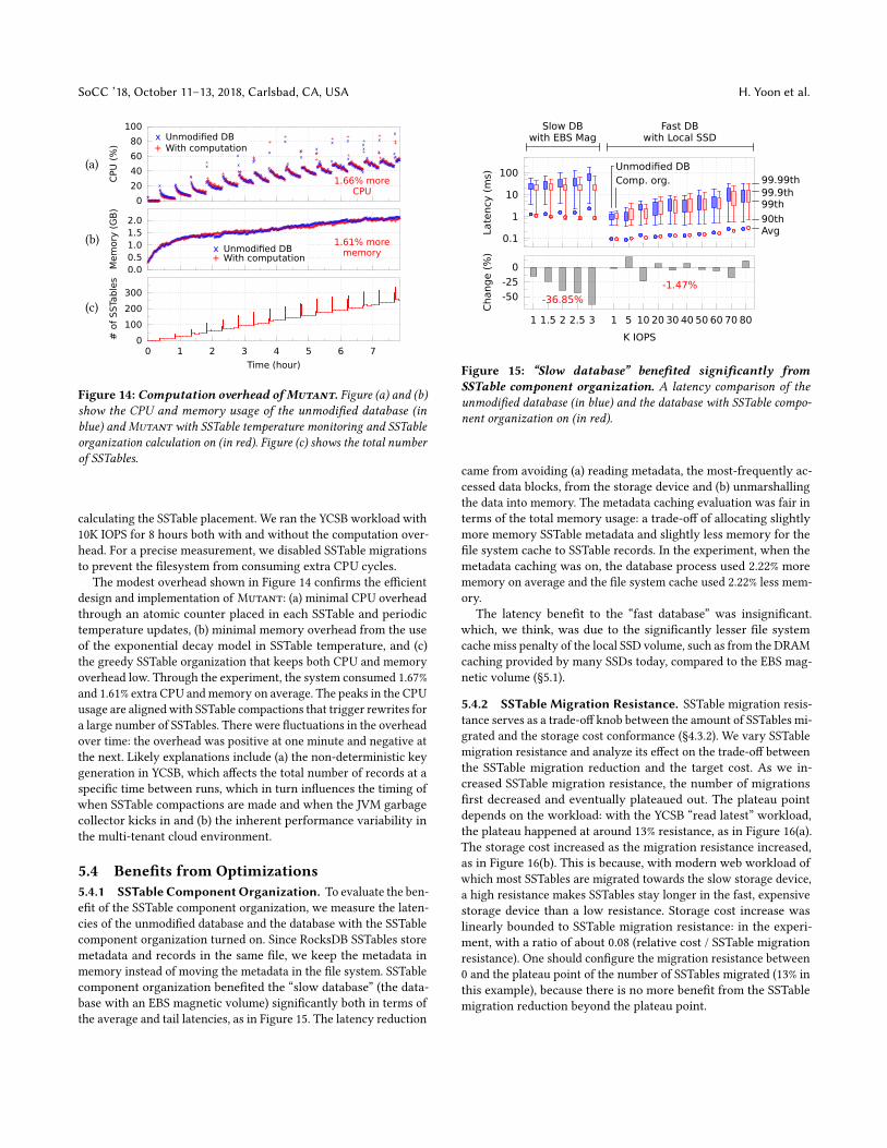
Figure 14: Computation overhead ofMutant. Figure (a) and (b)show the CPU and memory usage of the unmodified database (in
blue) andMutant with SSTable temperature monitoring and SSTable
organization calculation on (in red). Figure (c) shows the total number
of SSTables.
calculating the SSTable placement. We ran the YCSB workload with10K IOPS for 8 hours both with and without the computation over-head. For a precise measurement, we disabled SSTable migrationsto prevent the filesystem from consuming extra CPU cycles.
The modest overhead shown in Figure 14 confirms the efficientdesign and implementation of Mutant: (a) minimal CPU overheadthrough an atomic counter placed in each SSTable and periodictemperature updates, (b) minimal memory overhead from the useof the exponential decay model in SSTable temperature, and (c)the greedy SSTable organization that keeps both CPU and memoryoverhead low. Through the experiment, the system consumed 1.67%and 1.61% extra CPU andmemory on average. The peaks in the CPUusage are alignedwith SSTable compactions that trigger rewrites fora large number of SSTables. There were fluctuations in the overheadover time: the overhead was positive at one minute and negative atthe next. Likely explanations include (a) the non-deterministic keygeneration in YCSB, which affects the total number of records at aspecific time between runs, which in turn influences the timing ofwhen SSTable compactions are made and when the JVM garbagecollector kicks in and (b) the inherent performance variability inthe multi-tenant cloud environment.
5.4 Benefits from Optimizations5.4.1 SSTable ComponentOrganization. To evaluate the ben-efit of the SSTable component organization, we measure the laten-cies of the unmodified database and the database with the SSTablecomponent organization turned on. Since RocksDB SSTables storemetadata and records in the same file, we keep the metadata inmemory instead of moving the metadata in the file system. SSTablecomponent organization benefited the “slow database” (the data-base with an EBS magnetic volume) significantly both in terms ofthe average and tail latencies, as in Figure 15. The latency reduction
Slow DBwith EBS Mag
Fast DBwith Local SSD
0.1
1
10
100
1 1.5 2 2.5 3 1 5 10 20 30 40 50 60 70 80
Late
ncy
(m
s)
Unmodified DBComp. org. 99.99th
99.9th99th
90thAvg
-50
-25
0
1 1.5 2 2.5 3 1 5 10 20 30 40 50 60 70 80
Change (
%)
K IOPS
-36.85%
-1.47%
Figure 15: “Slow database” benefited significantly fromSSTable component organization. A latency comparison of the
unmodified database (in blue) and the database with SSTable compo-
nent organization on (in red).
came from avoiding (a) reading metadata, the most-frequently ac-cessed data blocks, from the storage device and (b) unmarshallingthe data into memory. The metadata caching evaluation was fair interms of the total memory usage: a trade-off of allocating slightlymore memory SSTable metadata and slightly less memory for thefile system cache to SSTable records. In the experiment, when themetadata caching was on, the database process used 2.22% morememory on average and the file system cache used 2.22% less mem-ory.
The latency benefit to the “fast database” was insignificant.which, we think, was due to the significantly lesser file systemcache miss penalty of the local SSD volume, such as from the DRAMcaching provided by many SSDs today, compared to the EBS mag-netic volume (§5.1).
5.4.2 SSTable Migration Resistance. SSTable migration resis-tance serves as a trade-off knob between the amount of SSTables mi-grated and the storage cost conformance (§4.3.2). We vary SSTablemigration resistance and analyze its effect on the trade-off betweenthe SSTable migration reduction and the target cost. As we in-creased SSTable migration resistance, the number of migrationsfirst decreased and eventually plateaued out. The plateau pointdepends on the workload: with the YCSB “read latest” workload,the plateau happened at around 13% resistance, as in Figure 16(a).The storage cost increased as the migration resistance increased,as in Figure 16(b). This is because, with modern web workload ofwhich most SSTables are migrated towards the slow storage device,a high resistance makes SSTables stay longer in the fast, expensivestorage device than a low resistance. Storage cost increase waslinearly bounded to SSTable migration resistance: in the experi-ment, with a ratio of about 0.08 (relative cost / SSTable migrationresistance). One should configure the migration resistance between0 and the plateau point of the number of SSTables migrated (13% inthis example), because there is no more benefit from the SSTablemigration reduction beyond the plateau point.

Mutant: Balancing Storage Cost and Latency in LSM-Tree Data Stores SoCC ’18, October 11–13, 2018, Carlsbad, CA, USA
(a)
0
50
100
150
200
0 5 10 15 20
SSTa
ble
sm
igra
ted (
GB
)
To fast storage
To slow storage
(b)
1.00
1.05
0 5 10 15 20
0.30
0.31
0.32
Sto
rage c
ost
(rela
tive t
o S
LO)
($/G
B/m
onth
)
SSTable migration resistance (%)
CostLinear regression of costsError range
Figure 16: SSTablemigration resistance’s effect on the SSTablemigrations and cost SLO conformance. Figure (a) shows how the
amount of SSTable migrations changes by SSTable migration resis-
tance, and (b) shows how the storage cost changes.
5.4.3 SSTable Compaction-Migration. SSTable compaction-migration integration is an optimization that piggybacks SSTablemigrations on SSTable compactions, thus reducing the amount ofSSTable migrations (§4.3.1). The breakdown of the SSTable com-pactions in Figure 17 shows that 20.37% of SSTable migrations weresaved from the integration. The number of SSTable compactionsremained consistent throughout the SSTable migration resistancerange, since the compactions were triggered solely by the leveledSSTable organizations, independent of the SSTable temperaturechanges.
6 RELATEDWORKLSM Tree Databases: LSM trees, invented by O’Neil [33], havebecome an attractive data structure for database systems in the pastdecade owing to their high write throughput and suitability forserving modern web workloads [1, 7, 16, 21, 25], These databasesorganize SSTables, the building blocks of a table, using variousstrategies that strike different read-write performance trade-offs:(a) size-tiered compaction used by BigTable, HBase, and Cassandra,(b) leveled compaction used by Cassandra, LevelDB, and RocksDB,(c) time window compaction used by Cassandra, and (d) universalcompaction used by RocksDB [4, 20]. Mutant uses leveled com-paction for its small SSTable sizes, which allows SSTables to beorganized across different storage types with minimal changes tothe underlying database. SSTable sizes under leveled compactionare 64 MiB in RocksDB or 160 MiB in Cassandra by default; withthe other compaction strategies, there is no upper bound on howmuch an SSTable can grow.
Optimizations to LSM tree databases include bLSM, which variesthe exponential fanout in the SSTable hierarchy to bound the num-ber of seeks [34], Partitioned Exponential Files that exploits prop-erties of HDD head schedulers [22], WiscKey that separates keysfrom values to reduce write amplification [29], and work of Limet al. that analyzes and optimizes the SSTable compaction param-eters [27]. These optimizations are orthogonal to how Mutantorganizes SSTables and can complement our approach.
0
50
100
0 5 10 15 20
SSTa
ble
sco
mpact
ed (
GB
)
SSTable migration resistance (%)
Regularcompactions
Compation-migrations20.37% of migrations saved20.37% of migrations saved20.37% of migrations saved20.37% of migrations saved20.37% of migrations saved20.37% of migrations saved20.37% of migrations saved20.37% of migrations saved20.37% of migrations saved20.37% of migrations saved20.37% of migrations saved20.37% of migrations saved20.37% of migrations saved20.37% of migrations saved20.37% of migrations saved20.37% of migrations saved20.37% of migrations saved20.37% of migrations saved20.37% of migrations saved20.37% of migrations saved20.37% of migrations saved20.37% of migrations saved20.37% of migrations saved20.37% of migrations saved20.37% of migrations saved20.37% of migrations saved20.37% of migrations saved20.37% of migrations saved20.37% of migrations saved20.37% of migrations saved20.37% of migrations saved20.37% of migrations saved20.37% of migrations saved20.37% of migrations saved20.37% of migrations saved20.37% of migrations saved20.37% of migrations saved20.37% of migrations saved20.37% of migrations saved20.37% of migrations saved20.37% of migrations saved20.37% of migrations saved20.37% of migrations saved20.37% of migrations saved20.37% of migrations saved20.37% of migrations saved20.37% of migrations saved20.37% of migrations saved20.37% of migrations saved20.37% of migrations saved20.37% of migrations saved20.37% of migrations saved20.37% of migrations saved20.37% of migrations saved20.37% of migrations saved20.37% of migrations saved20.37% of migrations saved20.37% of migrations saved20.37% of migrations saved20.37% of migrations saved20.37% of migrations saved20.37% of migrations saved20.37% of migrations saved20.37% of migrations saved20.37% of migrations saved20.37% of migrations saved20.37% of migrations saved20.37% of migrations saved20.37% of migrations saved20.37% of migrations saved20.37% of migrations saved20.37% of migrations saved20.37% of migrations saved20.37% of migrations saved20.37% of migrations saved20.37% of migrations saved20.37% of migrations saved20.37% of migrations saved20.37% of migrations saved20.37% of migrations saved20.37% of migrations saved20.37% of migrations saved20.37% of migrations saved20.37% of migrations saved20.37% of migrations saved
Figure 17: Breakdown of SSTable compactions by SSTable mi-gration resistance.
Multi-Storage, LSM Tree Databases: Several prior works useLSM tree databases across multiple storages. Time-series databasessuch as LHAM [32] splits the data at the the component (B+ tree)boundaries, storing lower level component in slower and cheaperstorages. RocksDB organizes SSTables by levels and store lower-level SSTables in slower and cheaper storages [6]. Cassandra storesSSTables to storages in a round-robin manner to guarantees evenusage of storage devices [3].
In comparison, the cost-performance trade-offs of these ap-proaches lack both configurability and versatility. First, databasesare deployed based on a static cost-performance trade-off, indepen-dent of the database’s lifetime. Any modifications and adjustmentsinvolve laborious data migration. Second, the trade-offs are lim-ited in options. Both with LHAM and RocksDB’s leveled SSTableorganization, the data is split in a coarse-grained manner. LHAMpartitions data at the the component (B+ tree) boundaries, leadingto only a small number of components since the components growexponentially in size. Leveled SSTable organization, which parti-tions data at the level boundaries, typically produces at most 4 to5 levels. Cassandra’s round-robin organization provides only oneoption, dividing SSTables evenly across storages.
These multi-storage, LSM tree database storage systems sharethe same idea asMutant: separating data into different storagesbased on their cost-performance characteristics. To the best of ourknowledge, however, Mutant is the first to provide a seamlesscost-performance trade-off, by taking advantage of the internalLSM tree-based database store layout, the data access locality frommodern web workloads, and the elastic cloud storage model.
7 CONCLUSIONSWe have presentedMutant: an LSM tree-based NoSQL databasestorage layer that delivers seamless cost-performance trade-offswith efficient algorithms that captures SSTable access popularity,organizes SSTables into different types of storage devices to meetthe changing target cost. Future work includes exploring (a) latencySLO enforcement in addition to the cost SLO enforcement and(b) finer-grained storage organization that addresses microscopic,record-level access frequency changes.
ACKNOWLEDGMENTWe would like to thank Avani Gadani, Helga Gudmundsdottir, andthe anonymous reviewers for their valuable suggestions and com-ments. This workwas supported byAWSCloud Credits for Researchprogram and NSF CAREER #1553579.

SoCC ’18, October 11–13, 2018, Carlsbad, CA, USA H. Yoon et al.
REFERENCES[1] 2016. Apache HBase. https://hbase.apache.org[2] 2017. Amazon EC2 Instance Types. https://aws.amazon.com/ec2/instance-types[3] 2017. Cassandra source code - Directories. https://github.com/apache/
cassandra/blob/684e250ba6e5b5bd1c246ceac332a91b2dc90859/src/java/org/apache/cassandra/db/Directories.java#L368
[4] 2017. DSE 5.1 Architecture Guide - How is data maintained?https://docs.datastax.com/en/dse/5.1/dse-arch/datastax_enterprise/dbInternals/dbIntHowDataMaintain.html
[5] 2017. QuizUp - The Biggest Trivia Game in theWorld. http://research.quizup.com[6] 2017. RocksDB source code - Compaction picker. https://github.com/facebook/
rocksdb/blob/e27f60b1c867b0b60dbff26d7a35777e6bb9f14b/db/compaction_picker.cc#L1286
[7] 2018. RocksDB - A persistent key-value store for fast storage environments.http://rocksdb.org
[8] Amazon Web Services. 2018. Amazon EBS Volume Types. https://docs.aws.amazon.com/AWSEC2/latest/UserGuide/EBSVolumeTypes.html
[9] Siddharth Anand. 2015. How big companies migrate from one database to another.https://www.quora.com/How-big-companies-migrate-from-one-database-to-another-without-losing-data-i-e-database-independent.
[10] Berk Atikoglu, Yuehai Xu, Eitan Frachtenberg, Song Jiang, and Mike Paleczny.2012. Workload analysis of a large-scale key-value store. In ACM SIGMETRICS
Performance Evaluation Review, Vol. 40. ACM, 53–64.[11] Shobana Balakrishnan, Richard Black, Austin Donnelly, Paul England, Adam
Glass, David Harper, Sergey Legtchenko, Aaron Ogus, Eric Peterson, andAntony IT Rowstron. 2014. Pelican: A Building Block for Exascale Cold DataStorage. In OSDI. 351–365.
[12] Theodore L Bergman and Frank P Incropera. 2011. Fundamentals of heat and
mass transfer. John Wiley & Sons.[13] Burton H Bloom. 1970. Space/time trade-offs in hash coding with allowable
errors. Commun. ACM 13, 7 (1970), 422–426.[14] Anders Brodersen, Salvatore Scellato, and Mirjam Wattenhofer. 2012. Youtube
around the world: geographic popularity of videos. In Proceedings of the 21st
international conference on World Wide Web. ACM, 241–250.[15] Brian Bulkowski. 2017. Amazon EC2 I3 Performance Results. https://www.
aerospike.com/benchmarks/amazon-ec2-i3-performance-results[16] Fay Chang, Jeffrey Dean, Sanjay Ghemawat, Wilson C Hsieh, Deborah A Wal-
lach, Mike Burrows, Tushar Chandra, Andrew Fikes, and Robert E Gruber. 2008.Bigtable: A distributed storage system for structured data. ACM Transactions on
Computer Systems (TOCS) 26, 2 (2008), 4.[17] Dennis Colarelli and Dirk Grunwald. 2002. Massive arrays of idle disks for storage
archives. In Proceedings of the 2002 ACM/IEEE conference on Supercomputing. IEEEComputer Society Press, 1–11.
[18] Brian F Cooper, Adam Silberstein, Erwin Tam, Raghu Ramakrishnan, and RussellSears. 2010. Benchmarking cloud serving systems with YCSB. In Proceedings of
the 1st ACM symposium on Cloud computing. ACM, 143–154.[19] Jonathan Ellis. 2011. Leveled Compaction in Apache Cassandra. http://www.
datastax.com/dev/blog/leveled-compaction-in-apache-cassandra
[20] Facebook. 2017. RocksDB Wiki - Compaction. https://github.com/facebook/rocksdb/wiki/Compaction
[21] Sanjay Ghemawat and Jeff Dean. 2017. LevelDB. https://github.com/google/leveldb
[22] Christopher Jermaine, Edward Omiecinski, and Wai Gen Yee. 2007. The parti-tioned exponential file for database storage management. The VLDB Journal-The
International Journal on Very Large Data Bases 16, 4 (2007), 417–437.[23] Jon Kleinberg and Eva Tardos. 2006. Algorithm design. Pearson Education India.[24] Sanjeev Kumar. 2014. Efficiency at Scale. International Workshop on Rack-scale
Computing (2014).[25] Avinash Lakshman and Prashant Malik. 2010. Cassandra: a decentralized struc-
tured storage system. ACM SIGOPS Operating Systems Review 44, 2 (2010), 35–40.[26] Jim Liddle. 2008. Amazon found every 100ms of latency cost them 1% in sales.
The GigaSpaces 27 (2008).[27] Hyeontaek Lim, David G Andersen, and Michael Kaminsky. 2016. Towards
Accurate and Fast Evaluation of Multi-Stage Log-structured Designs. In FAST.149–166.
[28] Steve Lohr. 2012. For Impatient Web Users, an Eye Blink Is JustToo Long to Wait. http://www.nytimes.com/2012/03/01/technology/impatient-web-users-flee-slow-loading-sites.html
[29] Lanyue Lu, Thanumalayan Sankaranarayana Pillai, Andrea C Arpaci-Dusseau,and Remzi H Arpaci-Dusseau. 2016. WiscKey: Separating Keys from Values inSSD-conscious Storage. In FAST. 133–148.
[30] Microsoft Azure. 2017. High-performance Premium Storage and managed disksfor VMs. https://docs.microsoft.com/en-us/azure/virtual-machines/windows/premium-storage
[31] Subramanian Muralidhar, Wyatt Lloyd, Sabyasachi Roy, Cory Hill, Ernest Lin,Weiwen Liu, Satadru Pan, Shiva Shankar, Viswanath Sivakumar, Linpeng Tang,et al. 2014. f4: Facebook’s warm BLOB storage system. In 11th USENIX Symposium
on Operating Systems Design and Implementation (OSDI 14). 383–398.[32] Peter Muth, Patrick O’Neil, Achim Pick, and Gerhard Weikum. 2000. The LHAM
log-structured history data access method. The VLDB Journal-The International
Journal on Very Large Data Bases 8, 3-4 (2000), 199–221.[33] Patrick O’Neil, Edward Cheng, Dieter Gawlick, and Elizabeth O’Neil. 1996. The
log-structured merge-tree (LSM-tree). Acta Informatica 33, 4 (1996), 351–385.[34] Russell Sears and Raghu Ramakrishnan. 2012. bLSM: a general purpose log
structured merge tree. In Proceedings of the 2012 ACM SIGMOD International
Conference on Management of Data. ACM, 217–228.[35] Amazon Web Services. 2017. Amazon EC2 Pricing. https://aws.amazon.com/
ec2/pricing[36] Amazon Web Services. 2018. Amazon EBS Pricing. https://aws.amazon.com/
ebs/pricing[37] Linpeng Tang, Qi Huang, Amit Puntambekar, Ymir Vigfusson, Wyatt Lloyd,
and Kai Li. 2017. Popularity Prediction of Facebook Videos for Higher Qual-ity Streaming. In 2017 USENIX Annual Technical Conference (USENIX ATC 17).USENIX Association.
[38] Mingyuan Xia, Mohit Saxena, Mario Blaum, and David Pease. 2015. A Tale ofTwo Erasure Codes in HDFS. In FAST. 213–226.