mvisumesh toolbox user's guide, version 0.0cuvelier/software/...mvisumesh toolbox user's...
TRANSCRIPT
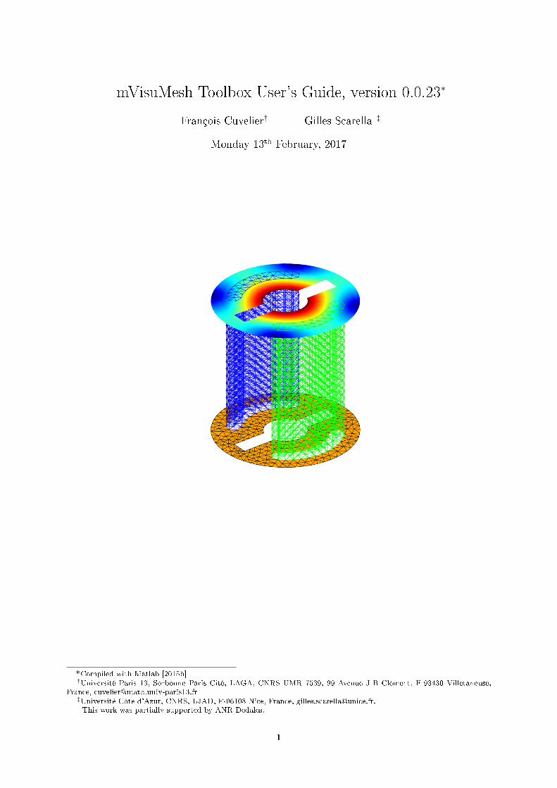
mVisuMesh Toolbox User's Guide, version 0.0.23˚
François Cuvelier: Gilles Scarella ;
Monday 13th February, 2017
˚Compiled with Matlab [2015b]:Université Paris 13, Sorbonne Paris Cité, LAGA, CNRS UMR 7539, 99 Avenue J-B Clément, F-93430 Villetaneuse,
France, [email protected];Université Côte d'Azur, CNRS, LJAD, F-06108 Nice, France, [email protected] work was partially supported by ANR Dedales.
1
Contents
1 Introduction 1
2 Installation of the toolbox 22.1 Installation by the .mltbx le . . . . . . . . . . . . . . . . . . . . . . . . . . . . . . . . . . 22.2 Installation by an archive le (.zip, .tar.gz or .7z) . . . . . . . . . . . . . . . . . . . . . . . 22.3 Meshes . . . . . . . . . . . . . . . . . . . . . . . . . . . . . . . . . . . . . . . . . . . . . . . 2
3 Initialization 23.1 Method with the .mltbx le . . . . . . . . . . . . . . . . . . . . . . . . . . . . . . . . . . . 23.2 Method with a typical archive le (.zip, .tar.gz or .7z) . . . . . . . . . . . . . . . . . . . . 23.3 Mesh samples . . . . . . . . . . . . . . . . . . . . . . . . . . . . . . . . . . . . . . . . . . . 2
4 Reading a mesh 34.1 About d-simplices . . . . . . . . . . . . . . . . . . . . . . . . . . . . . . . . . . . . . . . . . 34.2 Description of the mesh structure . . . . . . . . . . . . . . . . . . . . . . . . . . . . . . . . 34.3 Supported mesh types . . . . . . . . . . . . . . . . . . . . . . . . . . . . . . . . . . . . . . 54.4 GetMeshOpt function . . . . . . . . . . . . . . . . . . . . . . . . . . . . . . . . . . . . . . 6
5 Plotting a mesh 75.1 PlotMesh function . . . . . . . . . . . . . . . . . . . . . . . . . . . . . . . . . . . . . . . . 85.2 PlotBounds function . . . . . . . . . . . . . . . . . . . . . . . . . . . . . . . . . . . . . . . 115.3 PlotNodeNumber function . . . . . . . . . . . . . . . . . . . . . . . . . . . . . . . . . . . . 135.4 PlotTriangleNumber function . . . . . . . . . . . . . . . . . . . . . . . . . . . . . . . . . . 145.5 PlotEdgeNumber function . . . . . . . . . . . . . . . . . . . . . . . . . . . . . . . . . . . . 165.6 PlotBasisFunc function . . . . . . . . . . . . . . . . . . . . . . . . . . . . . . . . . . . . . 17
6 Representation of nodal variables 186.1 PlotVal function (2D) . . . . . . . . . . . . . . . . . . . . . . . . . . . . . . . . . . . . . . 186.2 PlotVal3D function . . . . . . . . . . . . . . . . . . . . . . . . . . . . . . . . . . . . . . . . 196.3 Plot3DSurfVal function . . . . . . . . . . . . . . . . . . . . . . . . . . . . . . . . . . . . . 216.4 PlotIsolines function (2D) . . . . . . . . . . . . . . . . . . . . . . . . . . . . . . . . . . . . 226.5 Plot3DSurfIsolines function . . . . . . . . . . . . . . . . . . . . . . . . . . . . . . . . . . . 24
7 Creating VTK les with vtkWrite function 257.1 Mesh representation in VTK format . . . . . . . . . . . . . . . . . . . . . . . . . . . . . . 257.2 Visualization of scalar or vector elds in VTK format . . . . . . . . . . . . . . . . . . . . 26
Abstract
mVisuMesh is a Matlab toolbox which allows to handle 2D and 3D simplicial meshes. Meshloading, mesh visualization and data visualization are enabled. Possible mesh formats are the onesof Triangle (2D), FreeFem++/medit (2D-3D) and gmsh (2D-3D).
1 Introduction
This toolbox allows to read and to handle simplicial meshes generated by gmsh [5], FreeFem++/medit[4, 7] or Triangle [10].
Meshes could be used by image processing, nite element or nite volume computations.Many functions are issued from mOptFEMP1 [1] and mVecFEMP1 [3, 2] packages (see François
Cuvelier's software page). Mesh reading and visualization have been extracted and improved from thesepackages to create the current package which is not specic to any research domain.
The toolbox has been tested from Matlab R2014a to R2016b. It has been tested under Linux (Ubuntu14.04, 16.04, Debian 7, 8, CentOS 7, OpenSUSE 13.2) and Mac OS X (El Capitan).
1

2 Installation of the toolbox
mVisuMesh toolbox may be installed from a .mltbx le or from a typical archive le (of extension .tar.gz,.zip or .7z). Some mesh samples are available to test the toolbox.
2.1 Installation by the .mltbx le
If the toolbox is downloaded as a .mltbx le, the user can install it directly by selecting it by the Openbutton in the Matlab window.
One may also run the script installmVisuMesh.m in Matlab, which does the same.
instal lmVisuMesh
The toolbox les are installed in the Matlab userpath, which depends on the Matlab version.
2.2 Installation by an archive le (.zip, .tar.gz or .7z)
If the toolbox is downloaded as an archive type of extension .tar.gz, .zip or .7z, the les need only to beextracted. The user may extract the archive anywhere he wants.
For example, with tar command,
ta r xvz f mVisuMesh´1 . 0 . 0 . ta r . gz
2.3 Meshes
Several meshes are used in demos. One needs to extract them from the mesh archive le meshes.tar.gzwhich can be downloaded with the toolbox.
ta r xvz f meshes . ta r . gz
3 Initialization
To use the toolbox the user needs to add the path of toolbox source les to his Matlab path.
3.1 Method with the .mltbx le
If the toolbox has been installed by the .mltbx le, toolbox source les are installed in the Matlabuserpath. For example, for a Linux machine with R2016a Matlab version, the user needs to do thefollowing
addpath ( '~/Documents/MATLAB/Add Ons/Toolboxes /mVisuMesh/code ' ) ;
For Matlab versions from R2014b and strictly before R2016a
addpath ( '~/Documents/MATLAB/Toolboxes /mVisuMesh/ ' ) ;
The user needs to add the paths of the toolbox subdirectories.
3.2 Method with a typical archive le (.zip, .tar.gz or .7z)
addpath ( '<path>/mVisuMesh/ ' ) ;
The user needs to add the paths of the toolbox subdirectories.
3.3 Mesh samples
The user needs to add the path of the mesh samples to his path.
2

4 Reading a mesh
In the toolbox only meshes composed of d-simplices are considered. A mesh structure close to the one inFreeFem++ is used in the toolbox.
4.1 About d-simplices
A d-simplex is made of pd`1q vertices. Most common d-simplices are the following:
• A 0-simplex is a node or a vertex.
• A 1-simplex is a segment.
• A 2-simplex is a triangle.
• A 3-simplex is a tetrahedron.
4.2 Description of the mesh structure
The data structure associated to a mesh employs many notations already used in FreeFem++ (see [7]).See also the report about the vecFEMP1 package [2].
3

Mesh structure associated to Thd : integer
simplex dimensiondim : integer
space dimensionnq : integer
number of verticesnme : integer
number of elements (d-simplices )nbe : integer
number of boundary elements ((d´1)-simplices )q : dim-by-nq array of reals
array of vertex coordinatesme : pd`1q-by-nme array of integers
connectivity array for mesh elementsmel : 1-by-nme array of integers
array of mesh element labelsbe : d-by-nbe array of integers
connectivity array for boundary elementsbel : 1-by-nbe array of integers
array of boundary element labelsvols : 1-by-nme array of reals
array of mesh element volumesh : double
mesh step size (=maximum edge length in the mesh)hmin : double
minimum edge length in the meshinfo : two eld structure
containing the name and the format of the mesh le
More precisely
• qpν, jq is the ν-th coordinate of the j-th vertex, ν P t1, . . . ,dimu, j P t1, . . . ,nqu. The j-th vertexwill be also denoted by qj “ qp:, jq.
• mepβ, kq is the storage index of the β-th vertex of the k-th element (d-simplex ), in the array q,for β P t1, ...,d ` 1u and k P t1, . . . ,nmeu. So qp:,mepβ, kqq represents the coordinates of the β-thvertex of the k-th mesh element.
• bepβ, lq is the storage index of the β-th vertex of the l-th boundary element ((d´1)-simplex ), inthe array q, for β P t1, ...,du and l P t1, . . . ,nbeu. So qp:,bepβ, lqq represents the coordinates of theβ-th vertex of the l-th boundary element.
• melpkq is the label of the k-th d-simplex .
• volspkq is the volume of the k-th d-simplex .
• info.name is a string of the short name of the mesh le (=relative path in Linux).info.format is the format of the mesh le: it can be 'freefem', 'medit' or 'gmsh'.
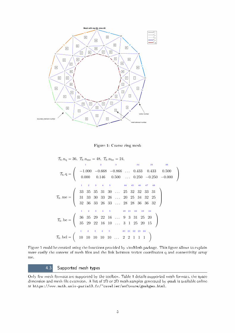
For example, we give in Figure 1 a ring mesh with 36 vertices, 48 mesh elements and 24 boundaryelements. The data structure associated to the mesh is denoted by Th and veries
4
1
2
3
4
5 6
7
8
9
10
11
1213
14
15
16
17
18
19
20
21
22
23
24
25
26
27
28
29 30
31
32
33
34
35
36
37
38
39
40
41
42
43
44
45
46
47
48
1
2
3
4
5
6
7
8
9
10
11
12
13
14
15
16
17
18
19
20
21
22
23
24
25
26
27
28
2930
31
32
33
34
35
36
22
23
2419
20
21
16
17
18 13
14
15
1
2
3 4
5
6
7
8
9 10
11
12
Mesh with nq=36, nme=48
Γ1
Γ2
Γ3
Γ4
Γ10
boundary element number
mesh element number
vertex number
Figure 1: Coarse ring mesh
Th.nq “ 36, Th.nme “ 48, Th.nbe “ 24,
Th.q “´1.000 ´0.668 ´0.866 . . . 0.433 0.433 0.500
0.000 0.146 0.500 . . . 0.250 ´0.250 ´0.000
¨
˝
˛
‚
1 2 3 34 35 36
Th.me “
33 35 35 31 30 . . . 25 32 32 33 31
31 33 30 33 26 . . . 20 25 34 32 25
32 36 33 26 33 . . . 28 28 36 36 32
¨
˚
˚
˝
˛
‹
‹
‚
1 2 3 4 5 44 45 46 47 48
Th.be “36 35 29 22 16 . . . 9 3 31 25 20
35 29 22 16 10 . . . 3 1 25 20 15
¨
˝
˛
‚
1 2 3 4 5 20 21 22 23 24
Th.bel “ 10 10 10 10 10 . . . 2 2 1 1 1
ˆ ˙
1 2 3 4 5 20 21 22 23 24
Figure 1 could be created using the functions provided by visuMesh package. This gure allows to explainmore easily the content of mesh les and the link between vertex coordinates q and connectivity arrayme.
4.3 Supported mesh types
Only few mesh formats are supported by the toolbox. Table 1 details supported mesh formats, the spacedimension and mesh le extension. A list of 2D or 3D mesh samples generated by gmsh is available onlineat https://www.math.univ-paris13.fr/~cuvelier/software/gmshgeo.html.
5
2D 3Dmesh software
mesh le extensionfreefem medit triangle gmsh.msh .mesh .msh
freefem/medit gmsh.mesh .msh
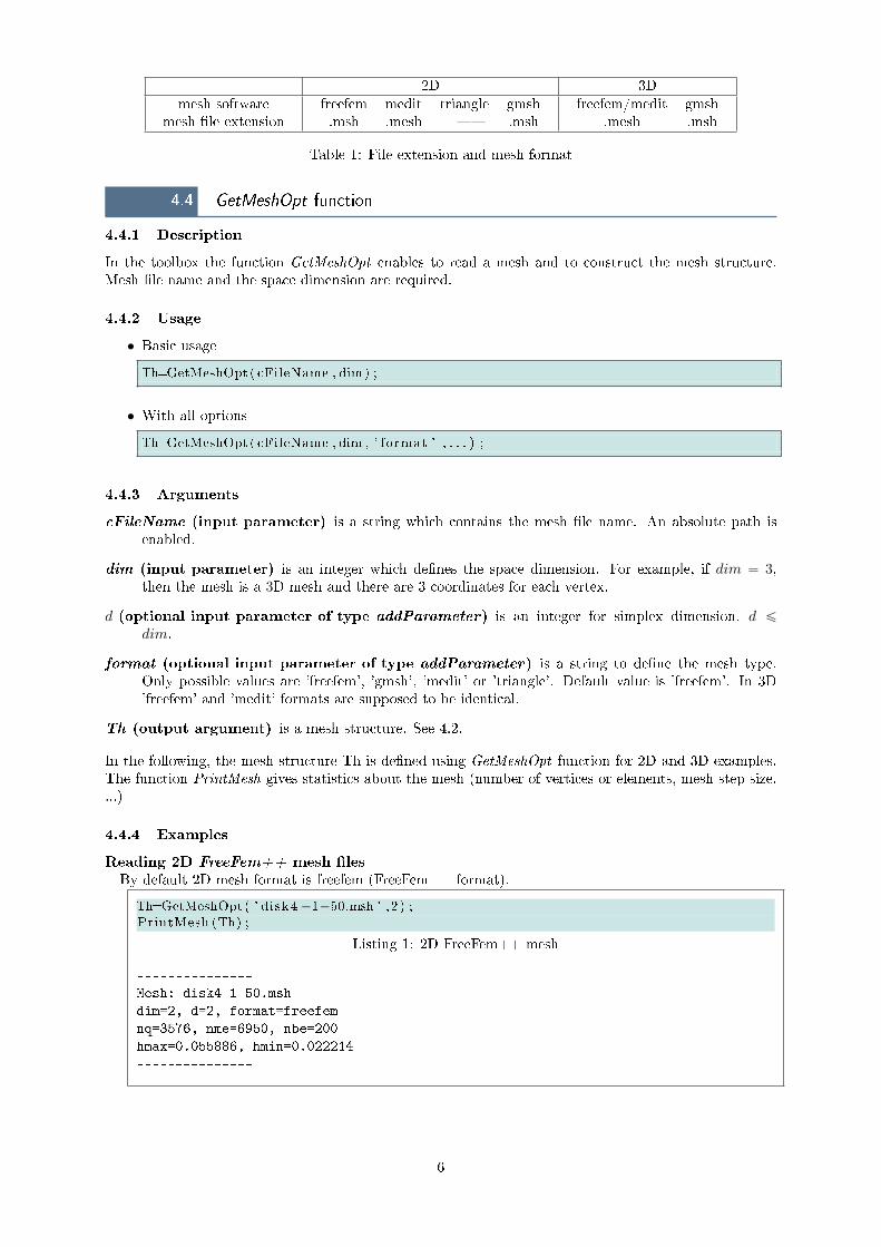
Table 1: File extension and mesh format
4.4 GetMeshOpt function
4.4.1 Description
In the toolbox the function GetMeshOpt enables to read a mesh and to construct the mesh structure.Mesh le name and the space dimension are required.
4.4.2 Usage
• Basic usage
Th=GetMeshOpt ( cFileName , dim) ;
• With all options
Th=GetMeshOpt ( cFileName , dim , ' format ' , . . . ) ;
4.4.3 Arguments
cFileName (input parameter) is a string which contains the mesh le name. An absolute path isenabled.
dim (input parameter) is an integer which denes the space dimension. For example, if dim “ 3,then the mesh is a 3D mesh and there are 3 coordinates for each vertex.
d (optional input parameter of type addParameter) is an integer for simplex dimension, d ď
dim.
format (optional input parameter of type addParameter) is a string to dene the mesh type.Only possible values are 'freefem', 'gmsh', 'medit' or 'triangle'. Default value is 'freefem'. In 3D'freefem' and 'medit' formats are supposed to be identical.
Th (output argument) is a mesh structure. See 4.2.
In the following, the mesh structure Th is dened using GetMeshOpt function for 2D and 3D examples.The function PrintMesh gives statistics about the mesh (number of vertices or elements, mesh step size,...)
4.4.4 Examples
Reading 2D FreeFem++ mesh lesBy default 2D mesh format is freefem (FreeFem++ format).
Th=GetMeshOpt ( ' disk4 ´1´50.msh ' , 2 ) ;PrintMesh (Th) ;
Listing 1: 2D FreeFem++ mesh
---------------
Mesh: disk4-1-50.msh
dim=2, d=2, format=freefem
nq=3576, nme=6950, nbe=200
hmax=0.055886, hmin=0.022214
---------------
6

Reading 2D Triangle mesh lesFor Triangle mesh les, the user has to set the format option as triangle.
Th=GetMeshOpt ( ' box . 1 ' , 2 , ' format ' , ' t r i a n g l e ' ) ;PrintMesh (Th) ;
Listing 2: 2D Triangle mesh
---------------
Mesh: box.1
dim=2, d=2, format=triangle
nq=12, nme=12, nbe=12
hmax=1.500000, hmin=1.000000
---------------
Reading 2D or 3D medit mesh les3D default mesh format is medit. Two examples for medit are given in the following, for each dimension
Th=GetMeshOpt ( ' rec t_bis2 . mesh ' ,2 , ...' format ' , ' medit ' ) ;
PrintMesh (Th) ;
Listing 3: 2D medit mesh
---------------
Mesh: rect_bis2.mesh
dim=2, d=2, format=medit
nq=2691, nme=5192, nbe=188
hmax=0.023424, hmin=0.009316
---------------
Th=GetMeshOpt ( ' cube6´1´3.mesh ' , 3 ) ;PrintMesh (Th) ;
Listing 4: 3D medit mesh
---------------
Mesh: cube6-1-3.mesh
dim=3, d=3, format=medit
nq=64, nme=162, nbe=108
hmax=0.577351, hmin=0.333333
---------------
Reading 2D or 3D gmsh mesh lesFor a gmsh le, the 'format' option with value 'gmsh' is required.
Th=GetMeshOpt ( 'magnetism .msh ' ,2 , ...' format ' , ' gmsh ' ) ;
PrintMesh (Th) ;
Listing 5: 2D gmsh mesh
---------------
Mesh: magnetism.msh
dim=2, d=2, format=gmsh
nq=1924, nme=3720, nbe=126
hmax=0.068956, hmin=0.022419
---------------
Th=GetMeshOpt ( ' sphere8 ´4.msh ' ,3 , ...' format ' , ' gmsh ' ) ;
PrintMesh (Th) ;
Listing 6: 3D gmsh mesh
---------------
Mesh: sphere8-4.msh
dim=3, d=3, format=gmsh
nq=1769, nme=7214, nbe=2022
hmax=0.322268, hmin=0.067119
---------------
5 Plotting a mesh
In this section some functions are introduced to represent a mesh and its boundaries. Some other functionsare also presented and can be used for debugging or for an educational purpose as they provide vertex,element or boundary element numbers. Here is the summary of the functions described in the section
PlotMesh function - To display a 2D or 3D mesh
PlotBounds function - To display the boundaries of a 2D or 3D mesh
PlotNodeNumber function - To display the node numbers in a 2D mesh
7

PlotTriangleNumber function - To display the triangle numbers in a 2D mesh
PlotEdgeNumber function - To display the boundary edge numbers in a 2D mesh
PlotBasicFunc function - To display the P1 basis function of a given vertex (only 2D)
5.1 PlotMesh function
5.1.1 Description
PlotMesh function allows to display a 2D or 3D mesh. The only required argument is the mesh structure.
5.1.2 Usage
• Basic usage
Th=GetMeshOpt ( . . . ) ;PlotMesh (Th) ;
• With all options
Th=GetMeshOpt ( . . . ) ;PlotMesh (Th, ' LineWidth ' , . . . , ' Color ' , . . . , ' RGBcolors ' , . . . , ...
' FaceAlpha ' , . . . , ' l a b e l s ' , . . . ) ;
5.1.3 Arguments
Th (input parameter) is a mesh structure (see 4.2)
Color (optional parameter of type addParameter) is a string which denes the color of meshlines. Default value is the empty string.
RGBcolors (optional parameter of type addParameter) is an array of RGB values (doubles be-tween 0 and 1) to set RGB values of the mesh lines. Each region may be identied by a dierentRGB. Default value is the empty array.
LineWidth (optional parameter of type addParameter) is a double which sets the line width ofmesh lines. Default value is 0.5.
FaceAlpha (optional parameter of type addParameter) is an integer which sets the transparency(only in 3D). 'FaceAlpha'=0 means no transparency. Default value is 0.
labels (optional parameter of type addParameter) is an array of labels (integer) to plot only spe-cic regions. Default value is the empty array.
Legend (optional parameter of type addParameter) is a boolean to display the legend or not.Default value is false. If true, the Ω symbol is used to denote each region.
No output argument
If both 'Color' and 'RGBcolors' are empty then RGBcolors prevails and is dened by the functionselect_colors of Timothy E. Holy - see [8] which allows to assign a dierent color to each subdomain.If both 'Color' and 'RGBcolors' are unempty then 'Color' prevails. As 'Color' is given by a string, it isconverted to an RGB value using the table given in Scalable Vector Graphics W3C web site.
5.1.4 Examples
Listings 7 and 8 show basic examples of using PlotMesh in 2D and 3D for a FreeFem++ and a Meditmesh respectively. Listings 9 and 10 deal with the use of LineWidth and RGBcolors options. Usingother options is similar. Listings 11 and 12 are examples of 2D and 3D meshes made of several physicaldomains.
8
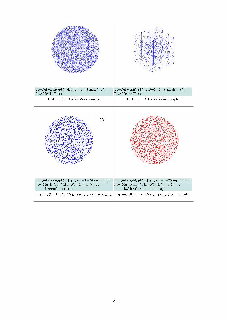
Th=GetMeshOpt ( ' disk4 ´1´50.msh ' , 2 ) ;PlotMesh (Th) ;
Listing 7: 2D PlotMesh sample
Th=GetMeshOpt ( ' cube6´1´3.mesh ' , 3 ) ;PlotMesh (Th) ;
Listing 8: 3D PlotMesh sample
Th=GetMeshOpt ( ' disque4 ´1´20.msh ' , 2 ) ;PlotMesh (Th, ' LineWidth ' , 1 . 0 , ...
' Legend ' , t rue ) ;
Listing 9: 2D PlotMesh sample with a legend
Th=GetMeshOpt ( ' disque4 ´1´20.msh ' , 2 ) ;PlotMesh (Th, ' LineWidth ' , 1 . 0 , ...
' RGBcolors ' , [ 1 0 0 ] )
Listing 10: 2D PlotMesh sample with a color
9

Th=GetMeshOpt ( 'magnetism .msh ' ,2 , ...' format ' , ' gmsh ' ) ;
PlotMesh (Th) ;
Listing 11: 2D PlotMesh sample
Th=GetMeshOpt ( ...' FlowVelocity3d01 ´3.mesh ' , 3 ) ;
PlotMesh (Th) ;
Listing 12: 3D PlotMesh sample
In Listing 14 only labels 8 and 12 are shown (to be compared with Listing 12).
Th=GetMeshOpt ( 'magnetism .msh ' ,2 , ...' format ' , ' gmsh ' ) ;
PlotMesh (Th, ' l a b e l s ' , [ 3 ...4 ] , ' Legend ' , t rue ) ;
Listing 13: 2D PlotMesh using labels option
Th=GetMeshOpt ( ...' FlowVelocity3d01 ´3.mesh ' , 3 ) ;
PlotMesh (Th, ' l a b e l s ' , [ 8 ...1 2 ] , ' Legend ' , t rue ) ;
Listing 14: 3D PlotMesh using labels option
10

5.2 PlotBounds function
5.2.1 Description
PlotBounds function allows to display the boundaries of a 2D or 3D mesh. The only required argumentis the mesh structure.
5.2.2 Usage
• Basic usage
Th=GetMeshOpt ( . . . ) ;PlotBounds (Th) ;
• With all options
Th=GetMeshOpt ( . . . ) ;r gbco l=PlotBounds (Th, ' LineWidth ' , . . . , ' Color ' , . . . , ...
' RGBcolors ' , . . . , ' Legend ' , . . . , ' FontSize ' , . . . , ' l a b e l s ' , . . . ) ;
5.2.3 Arguments
Th (input parameter) is a mesh structure (see 4.2)
LineWidth (optional parameter of type addParameter) is a double which sets the line width ofboundaries (only in 2D). Default value is 2.
Color (optional parameter of type addParameter) is a string which denes the color of bound-aries. Default value is the empty string.
RGBcolors (optional parameter of type addParameter) is an array of RGB values (doubles be-tween 0 and 1) to set RGB values of the boundaries. Each boundary may be identied by a dierentRGB. Default value is the empty array.
Legend (optional parameter of type addParameter) is a bool to display the legend or not. De-fault value is true. The Γ symbol is used to denote each boundary.
FontSize (optional parameter of type addParameter) is an integer to set the font size of the leg-end. Default value is 10.
labels (optional parameter of type addParameter) is an array of labels (integer) to plot only spe-cic regions.
rgbcol optional output argument is the array of the RGB colors used by the plot. Default value isthe empty array.
If 'Color' and 'RGBcolors' are both empty, as for PlotMesh in 5.1 then RGBcolors prevails and isdened by the function select_colors of Timothy E. Holy - see [8] which allows to set a dierent color toeach subdomain. If both 'Color' and 'RGBcolors' are unempty then Color prevails. If 'Color' is given bya string, it is converted to an RGB value using the table given in Scalable Vector Graphics W3C web ite
5.2.4 Examples
Listings 15 and 16 show basic examples of using PlotBounds in 2D and 3D. Listing 17 deals with the useof Color option. Using other options is similar. Listing 20 is an example of the labels option for a 3Dmesh. Listings 18 and 19 show examples combining PlotMesh and PlotBounds functions and also the useof labels option. In gures of Listings 18, 19, and 21 it is not possible to have legends for both domainsand boundaries.
11

Th=GetMeshOpt ( ' disk4 ´1´50.msh ' , 2 ) ;PlotBounds (Th) ;
Listing 15: 2D PlotBounds sample
Th=GetMeshOpt ( ' sphere8 ´4.msh ' ,3 , ...' format ' , ' gmsh ' ) ;
PlotBounds (Th) ;axis image ;
Listing 16: 3D PlotBounds sample
Th=GetMeshOpt ( ' sphere8 ´4.msh ' ,3 , ' format ' , ' gmsh ' ) ;PlotBounds (Th, ' Color ' , ' red ' , ' Legend ' , f a l s e ) ;axis image ;
Listing 17: 3D PlotBounds sample in only red color
12

Th=GetMeshOpt ( 'magnetism .msh ' ,2 , ...' format ' , ' gmsh ' ) ;
PlotBounds (Th, ' Color ' , ' b lack ' ) ;PlotMesh (Th, ' l a b e l s ' , [ 3 , 4 ] ) ;
Listing 18: PlotMesh+PlotBounds sample
Th=GetMeshOpt ( ' disk4 ´1´50.msh ' , 2 ) ;PlotMesh (Th) ;PlotBounds (Th, ' l a b e l s ' , [ 1 , 2 ] , ...
' RGBcolors ' , [ 1 , 0 , 0 ; 0 , 1 , 0 ] ) ;
Listing 19: PlotBounds+ PlotMesh sample
Th=GetMeshOpt ( ' cy l inderkey ´10.msh ' , ...3 , ' format ' , ' gmsh ' ) ;
PlotBounds (Th, ' l a b e l s ' , [ 1 0 11 1000 ...1020 1021 2000 2020 2021 ] ) ;
axis image ;
Listing 20: 3D PlotBounds sample
Th=GetMeshOpt ( ...' FlowVelocity3d01 ´3.mesh ' , 3 ) ;
PlotBounds (Th, ' l a b e l s ' , [ 1000 1020 ...1021 2000 2020 2021 ] ) ;
PlotMesh (Th, ' l a b e l s ' , [ 8 , 1 2 ] ) ;
Listing 21: PlotBounds+ PlotMesh sample
5.3 PlotNodeNumber function
5.3.1 Description
PlotNodeNumber function allows to display numbers of nodes in a mesh. The only required argument isthe mesh structure. This function could be useful for debugging or for an educational purpose.
The function is limited to the 2D case and should be used for meshes containing few vertices.
5.3.2 Usage
• Basic usage
Th=GetMeshOpt ( . . . ) ;PlotNodeNumber (Th) ;
13

• With all options
Th=GetMeshOpt ( . . . ) ;PlotNodeNumber (Th, ' BackgroundColor ' , . . . , ' FontSize ' , . . . , ' Color ' , . . . , 'C ' , . . . ) ;
5.3.3 Arguments
Th (input parameter) is a mesh structure (see 4.2)
BackgroundColor (optional parameter of type addParameter) is a RGB value which sets thebackground color. Default value is [1 1 1] (white).
FontSize (optional parameter of type addParameter) is an integer to set the font size of nodenumbers. Default value is 10.
Color (optional parameter of type addParameter) is a RGB value (doubles between 0 and 1) toset RGB value of the number color. Default value is [0 0 0] (black).
C (optional parameter of type addParameter) is an integer equal to the shift for node numbering(equal to 0 or 1). Default value is 0. If C=0, node numbering goes from 1 to Th.nq else from 0 toTh.nq-1.
No output argument
5.3.4 Examples
Listing 22 is an example of using PlotNodeNumber combined with PlotMesh.
Th=GetMeshOpt ( ' disque4 ´1´4.msh ' , 2 ) ;PlotMesh (Th, ' Color ' , ' brown ' )PlotNodeNumber (Th, ' Color ' , [ 0 0 ...
0 ] , ' FontSize ' , 22) ;
Listing 22: PlotNodeNumber sample
5.4 PlotTriangleNumber function
5.4.1 Description
PlotTriangleNumber function allows to display triangle numbers in a 2D mesh. The only required argu-ment is the mesh structure. This function could be useful for debugging or for an educational purpose.A call to the function PlotMesh is required before the call to PlotTriangleNumber.
The function is limited to the 2D case and should be used for meshes containing few triangularelements.
14

5.4.2 Usage
• Basic usage
Th=GetMeshOpt ( . . . ) ;PlotTriangleNumber (Th) ;
• With all options
Th=GetMeshOpt ( . . . ) ;PlotTriangleNumber (Th, ' BackgroundColor ' , . . . , ' FontSize ' , . . . , ' Color ' , . . . , ...
' EdgeColor , . . . , 'C ' , . . . ) ;
5.4.3 Arguments
Th (input parameter) is a mesh structure (see 4.2)
BackgroundColor (optional parameter of type addParameter) is a RGB value which sets thebackground color. Default value is [1 1 1] (white).
FontSize (optional parameter of type addParameter) is an integer to set the font size of trianglenumbers. Default value is 10.
Color (optional parameter of type addParameter) is a RGB value (doubles between 0 and 1) toset RGB value of the number color. Default value is [0 0 0] (black).
EdgeColor (optional parameter of type addParameter) is a RGB value (doubles between 0 and1) to set RGB value of the number color on edges. Default value is [0 0 0] (black).
C (optional parameter of type addParameter) is an integer equal to 0 or 1 for the numbering shift(if C=1, numbering starts from 0). Default value is 0.
No output argument
5.4.4 Examples
Listing 23 is an example of using PlotTriangleNumber combined with PlotMesh. Listing 24 depicts amore complete example including PlotMesh, PlotNodeNumber and PlotTriangleNumber.
Th=GetMeshOpt ( ' disque4 ´1´3.msh ' , 2 ) ;PlotMesh (Th) ;PlotTriangleNumber (Th, ' Color ' , [ 1 0 ...
0 ] , ' FontSize ' , 22) ;
Listing 23: PlotTriangleNumber sample
Th=GetMeshOpt ( ' disque4 ´1´3.msh ' , 2 ) ;PlotMesh (Th, ' Color ' , ' brown ' ) ;PlotNodeNumber (Th, ' FontSize ' , 16) ;PlotTriangleNumber (Th, ' Color ' , [ 1 0 ...
0 ] , ' FontSize ' , 22) ;
Listing 24: PlotTriangleNumber+PlotNodeNumber sample
15

5.5 PlotEdgeNumber function
5.5.1 Description
PlotEdgeNumber function allows to display boundary edge numbers in a 2D mesh. The only requiredargument is the mesh structure. This function could be useful for debugging or for an educational purpose.A call to the function PlotMesh is required before the call to PlotEdgeNumber.
The function is limited to the 2D case.
5.5.2 Usage
• Basic usage
Th=GetMeshOpt ( . . . ) ;PlotEdgeNumber (Th) ;
• With all options
Th=GetMeshOpt ( . . . ) ;PlotEdgeNumber (Th, 'RGBTextColors ' , . . . , 'RGBEdgeColors ' , . . . , ...
' BackgroundColor ' , . . . , ' FontSize ' , . . . , ' FontWeight ' , . . . , ' Color ' , . . . , ...' EdgeColor ' , . . . , ' LineWidth ' , . . . , ' L ineSty l e ' , . . . ) ;
5.5.3 Arguments
Th (input parameter) is a mesh structure (see 4.2)
RGBTextColors (optional parameter of type addParameter) sets the RGB color of boundaryedge numbers. Default value is an empty array.
RGBEdgeColors (optional parameter of type addParameter) sets the RGB color of boundarybox edge numbers. Default value is an empty array.
BackgroundColor (optional parameter of type addParameter) is a RGB value which sets theboundary edge number background box color. Default value is [1 1 1] (white).
FontSize (optional parameter of type addParameter) is an integer to set the font size of bound-ary node numbers. Default value is 10.
FontWeight (optional parameter of type addParameter) is a string to dene set the boundaryedge number font weight as 'normal', 'bold','light' or 'demi'. Default value is 'normal'.
Color (optional parameter of type addParameter) is a RGB value (doubles between 0 and 1) toset RGB value of the number color. Default value is [0 0 0] (black).
EdgeColor (optional parameter of type addParameter) is a RGB value (doubles between 0 and1) to set RGB value of the number color on edges. Default value is [0 0 0] (black).
LineWidth (optional parameter of type addParameter) is a double which sets the line width ofmesh lines. Default value is 0.5.
LineStyle (optional parameter of type addParameter) sets the line style of mesh lines to 'none','-','','.' or '-.' Default value is 'none'.
No output argument
5.5.4 Examples
Listing 25 is an example of using PlotEdgeNumber combined with PlotMesh. Listing 26 depicts a morecomplete example including PlotMesh, PlotBounds, PlotNodeNumber and PlotTriangleNumber functions.This example corresponds to the Figure 1 which explains the mesh structure (see also 4.2).
16

Th=GetMeshOpt ( ' disque4 ´1´4.msh ' , 2 ) ;PlotMesh (Th) ;PlotEdgeNumber (Th, ' Color ' , [ 1 0 ...
0 ] , ' FontSize ' , 16) ;
Listing 25: PlotEdgeNumber sample
Th=GetMeshOpt ( 'Ring´3.msh ' , 2 ) ;PlotMesh (Th, ' RGBcolors ' , ...
s e l e c tCo l o r s ( length ( ...unique (Th . be l ) )+1) ) ;
RGBcolors=PlotBounds (Th, ' FontSize ' , 15) ;PlotEdgeNumber (Th, 'RGBEdgeColors ' , ...
RGBcolors , ' Color ' , [ 0 0 ...0 ] , ' L ineSty l e ' , '´ ' , ...' LineWidth ' , 0 . 5 , ' FontSize ' , 12) ;
PlotNodeNumber (Th, ' Color ' , [ 0 0 ...1 ] , ' FontSize ' , 12) ;
PlotTriangleNumber (Th, ' Color ' , [ 1 0 ...0 ] , ' FontSize ' , 12) ;
Listing 26: PlotEdgeNumber+PlotNodeNumber+ PlotTriangleNumbersample
5.6 PlotBasisFunc function
5.6.1 Description
PlotBasisFunc function allows to display the P1 basis function of a given vertex. The mesh structureand the vertex number are required. This function could be useful for debugging or for an educationalpurpose.
The function is limited to the 2D case.
5.6.2 Usage
• Basic usage
Th=GetMeshOpt ( . . . ) ;n = . . . ;PlotBasisFunc (Th, n) ;
5.6.3 Arguments
Th (input parameter) is a mesh structure (see 4.2)
n (input parameter) vertex number for which the basis function is displayed
No output argument
17

5.6.4 Examples
Th=GetMeshOpt ( ' disque4 ´1´3.msh ' , 2 ) ;n=15; PlotBasisFunc (Th, n) ;
Listing 27: 2D PlotBasisFunc sample
6 Representation of nodal variables
In this section some functions are introduced to represent nodal elds on a mesh and its boundaries (only3D). Here is the summary of the functions described in the section
PlotVal function - To represent a nodal eld on a 2D mesh.
PlotVal3D function - To represent a nodal eld on a 3D mesh
Plot3DSurfVal function - To represent a nodal eld on the boundaries of a 3D mesh.
PlotIsolines function - To display isolines of a scalar eld in 2D.
Plot3DSurfIsolines function - To display isolines of a scalar eld on the boundaries of a 3D mesh.
6.1 PlotVal function (2D)
6.1.1 Description
PlotVal function allows to display a nodal eld in 2D. Required arguments are the mesh structure andthe eld u. u is an array of doubles of size nq.
6.1.2 Usage
• Basic usage
Th=GetMeshOpt ( . . . ) ;u = . . . ;PlotVal (Th, u) ;
• With all options
18
Th=GetMeshOpt ( . . . ) ;u = . . . ;h=PlotVal (Th, u , ' CameraPosition ' , . . . , ' colormap ' , . . . , ...
' shading ' , . . . , ' c o l o rba r ' , . . . , ' c ax i s ' , . . . , ' l a b e l s ' , . . . ) ;
6.1.3 Arguments
Th (input parameter) is a mesh structure (see 4.2)
Val (input parameter) is an array of doubles of size Th.nq
CameraPosition (optional parameter of type addParameter) is an array of two doubles to setthe camera position. Default value is view(2).
colormap (optional parameter of type addParameter) is a colormap value. Default value is 'jet'.
shading (optional parameter of type addParameter) is a bool to use 'shading interp' or not. De-fault value is true.
colorbar (optional parameter of type addParameter) is a bool to display the colorbar or not.Default value is true.
caxis (optional parameter of type addParameter) is an array of four doubles to set the axis. De-fault value is an empty array.
labels (optional parameter of type addParameter) is an array of labels (integer) to plot the eldon specic regions.
h optional output argument returns the handle to the gure
6.1.4 Examples
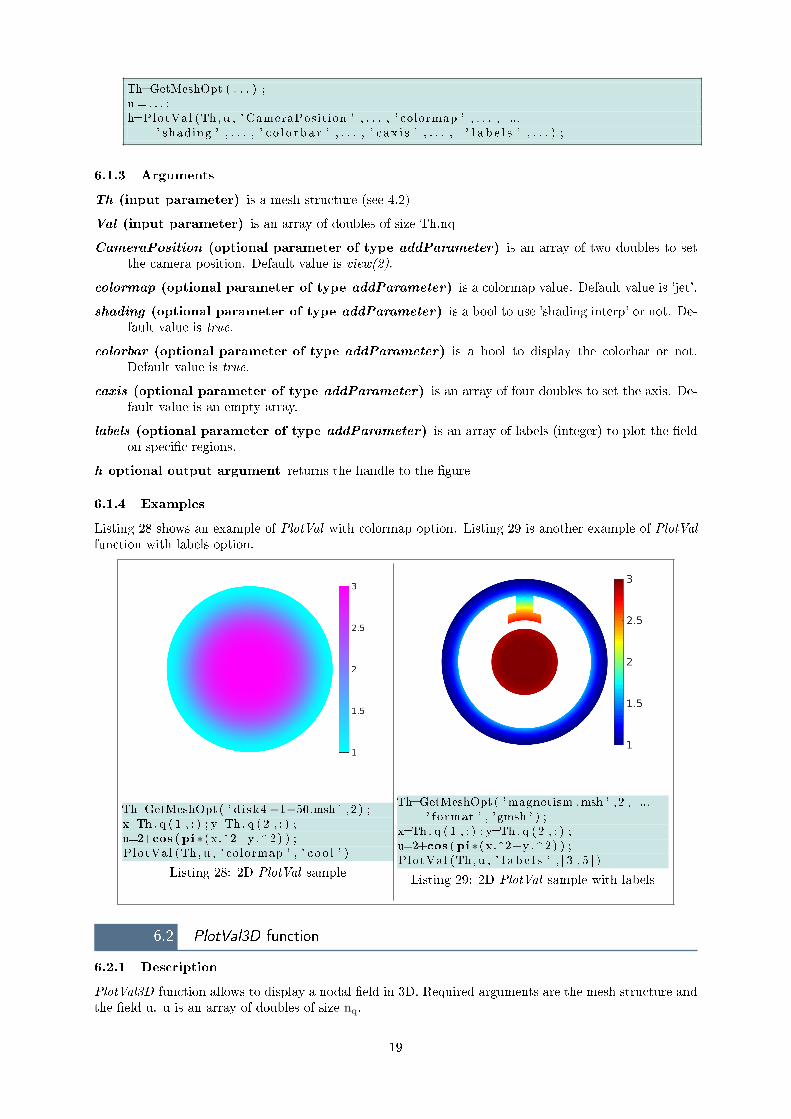
Listing 28 shows an example of PlotVal with colormap option. Listing 29 is another example of PlotValfunction with labels option.
Th=GetMeshOpt ( ' disk4 ´1´50.msh ' , 2 ) ;x=Th . q ( 1 , : ) ; y=Th . q ( 2 , : ) ;u=2+cos (pi ∗( x.^2+y .^2) ) ;PlotVal (Th, u , ' colormap ' , ' c oo l ' )
Listing 28: 2D PlotVal sample
Th=GetMeshOpt ( 'magnetism .msh ' ,2 , ...' format ' , ' gmsh ' ) ;
x=Th . q ( 1 , : ) ; y=Th . q ( 2 , : ) ;u=2+cos (pi ∗( x.^2+y .^2) ) ;PlotVal (Th, u , ' l a b e l s ' , [ 3 , 5 ] )
Listing 29: 2D PlotVal sample with labels
6.2 PlotVal3D function
6.2.1 Description
PlotVal3D function allows to display a nodal eld in 3D. Required arguments are the mesh structure andthe eld u. u is an array of doubles of size nq.
19

6.2.2 Usage
• Basic usage
u = . . . ;PlotVal3D (Th, u) ;
• With all options
Th=GetMeshOpt ( . . . ) ;u = . . . ;h=PlotVal3D (Th, u , ' colormap ' , . . . , ' shading ' , . . . , ' c o l o rba r ' , . . . , ...
' c ax i s ' , . . . , ' PlotOptions ' , . . . ) ;
6.2.3 Arguments
Th (input parameter) is a mesh structure (see 4.2)
u (input parameter) array of doubles of size Th.nq
colormap (optional parameter of type addParameter) is a colormap value. Default value is 'jet'.
shading (optional parameter of type addParameter) is a bool to use 'shading interp' or not. De-fault value is true.
colorbar (optional parameter of type addParameter) is a bool to display the colorbar or not.Default value is true.
caxis (optional parameter of type addParameter) is an array of four doubles to set the axis. De-fault value is an empty array.
PlotOptions (optional parameter of type addParameter) is a cell for dening plotting options.Default value is an empty cell.
h optional output argument returns the handle to the gure
6.2.4 Examples
Listing 30 is a basic example of PlotVal3D.
Th=GetMeshOpt ( ' cy l inderkey ´10.msh ' ,3 , ...' format ' , ' gmsh ' ) ;
f=@(x , y , z ) x.^2+y.^2+cos ( ( z´1) .^2) ;U=f (Th . q ( 1 , : ) ,Th . q ( 2 , : ) ,Th . q ( 3 , : ) ) ;PlotVal3D (Th,U) ;
Listing 30: PlotVal3D sample
20

6.3 Plot3DSurfVal function
6.3.1 Description
Plot3DSurfVal allows to represent a nodal eld on the surface of a 3D mesh. Required arguments arethe mesh structure and the eld u. u is an array of doubles of size nq.
6.3.2 Usage
• Basic usage
Th=GetMeshOpt ( . . . ) ;u = . . . ;Plot3DSurfVal ( . . . ) ;
• With all options
Th=GetMeshOpt ( . . . ) ;u = . . . ;Plot3DSurfVal (Th, u , ' colormap ' , . . . , ' c o l o rba r ' , . . . , ...
' l a b e l s ' , . . . , ' PlotOptions ' , . . . ) ;
6.3.3 Arguments
Th (input parameter) is a mesh structure (see 4.2)
u (input parameter) array of doubles of size Th.nq
colormap (optional parameter of type addParameter) is a colormap value. Default value is 'jet'.
colorbar (optional parameter of type addParameter) is a bool to display the colorbar or not.Default value is true.
labels (optional parameter of type addParameter) is an array of labels (integer) to represent theeld only on specic boundaries.
PlotOptions (optional parameter of type addParameter) is a cell for dening plotting options.Default value is an empty cell.
No output argument
6.3.4 Examples
The gure in Listing 31 shows the representation of a eld on a sphere. The Figure in Listing 32 representsthe same except there is no EdgeColor as required by PlotOptions. Figure in Listing 33 represents thesame but shows only some regions as labels option is used. Figure in Listing 34 represents the samegure as the rst page of the report, combining the use of PlotMesh, PlotBounds and Plot3DSurfValfunctions.
21
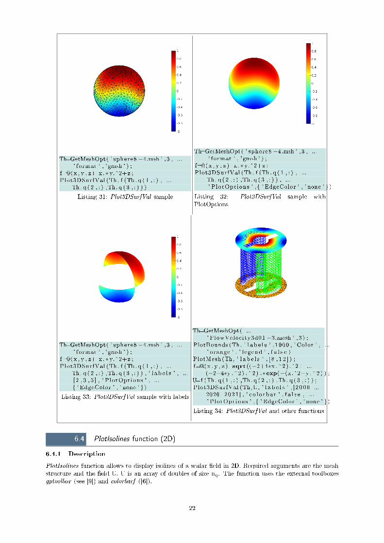
Th=GetMeshOpt ( ' sphere8 ´4.msh ' ,3 , ...' format ' , ' gmsh ' ) ;
f=@(x , y , z ) x .∗ y.^2+z ;Plot3DSurfVal (Th, f (Th . q ( 1 , : ) , ...
Th . q ( 2 , : ) ,Th . q ( 3 , : ) ) )
Listing 31: Plot3DSurfVal sample
Th=GetMeshOpt ( ' sphere8 ´4.msh ' ,3 , ...' format ' , ' gmsh ' ) ;
f=@(x , y , z ) x .∗ y.^2+z ;Plot3DSurfVal (Th, f (Th . q ( 1 , : ) , ...
Th . q ( 2 , : ) ,Th . q ( 3 , : ) ) , ...' PlotOptions ' , ' EdgeColor ' , ' none ' )
Listing 32: Plot3DSurfVal sample withPlotOptions
Th=GetMeshOpt ( ' sphere8 ´4.msh ' ,3 , ...' format ' , ' gmsh ' ) ;
f=@(x , y , z ) x .∗ y.^2+z ;Plot3DSurfVal (Th, f (Th . q ( 1 , : ) , ...
Th . q ( 2 , : ) ,Th . q ( 3 , : ) ) , ' l a b e l s ' , ...[ 2 , 3 , 5 ] , ' PlotOptions ' , ... ' EdgeColor ' , ' none ' )
Listing 33: Plot3DSurfVal sample with labels
Th=GetMeshOpt ( ...' FlowVelocity3d01 ´3.mesh ' , 3 ) ;
PlotBounds (Th, ' l a b e l s ' ,1000 , ' Color ' , ...' orange ' , ' l egend ' , f a l s e )
PlotMesh (Th, ' l a b e l s ' , [ 8 , 1 2 ] ) ;f=@(x , y , z ) sqrt ((´2+4∗x .^2) .^2+ ...
(´2+4∗y .^2) .^2) .∗exp(´(x.^2+y .^2) ) ;U=f (Th . q ( 1 , : ) ,Th . q ( 2 , : ) ,Th . q ( 3 , : ) ) ;Plot3DSurfVal (Th,U, ' l a b e l s ' , [ 2000 ...
2020 2021 ] , ' c o l o rba r ' , f a l s e , ...' PlotOptions ' , ' EdgeColor ' , ' none ' )
Listing 34: Plot3DSurfVal and other functions
6.4 PlotIsolines function (2D)
6.4.1 Description
PlotIsolines function allows to display isolines of a scalar eld in 2D. Required arguments are the meshstructure and the eld U. U is an array of doubles of size nq. The function uses the external toolboxesgptoolbox (see [9]) and colorbarf ([6]).
22
6.4.2 Usage
• Basic usage
Th=GetMeshOpt ( . . . ) ;U= . . . ;P l o t I s o l i n e s (Th,U) ;
• With all options
Th=GetMeshOpt ( . . . ) ;U= . . . ;[ co l , i s o r ]= P l o t I s o l i n e s (Th,U, ' n i s o ' , . . . , ' colormap ' , . . . , ' c o l o rba r ' , . . . , ...
' PlotOptions ' , . . . , ' i s o r ange ' , . . . , ' l a b e l s ' , . . . ) ;
6.4.3 Arguments
Th (input parameter) is a mesh structure (see 4.2)
U (input parameter) array of doubles of size Th.nq
niso (optional parameter of type addParameter) is an integer which sets the number of isolinesto be plotted. Default value is 10.
colormap (optional parameter of type addParameter) is a colormap value. Default value is 'jet'.
colorbar (optional parameter of type addParameter) is a bool to display the colorbar or not.Default value is false.
PlotOptions (optional parameter of type addParameter) is a cell for dening plotting options.Default value is an empty cell.
plan (optional parameter of type addParameter) (bool) To plot isolines in 2D in the xOy-plane(if true) or in 3D (if false). Default value is false.
isorange (optional parameter of type addParameter) is an array of integers which denes theisoline values. Default value is an empty array and niso isoline values are set in proportion in therange of minimum and maximum values.
labels (optional parameter of type addParameter) is an array of labels (integer) to plot only spe-cic regions. Default value is an empty array.
[col,isor] optional output arguments . col is the array of RGB colors used by the plot. isor is thearray of isoline values.
PlotIsolines allows to plot isolines for a 2D variable.
6.4.4 Examples
The gure in Listing 35 displays isolines of a 2D eld using colorbar and PlotOptions option. TheFigure in Listing 36 represents the same but it also gives the 3D representation of the eld using trisurffunction.
23

Th=GetMeshOpt ( ' disk4 ´1´50.msh ' , 2 ) ;x=Th . q ( 1 , : ) ; y=Th . q ( 2 , : ) ;u=2+cos (pi ∗( x.^2+y .^2) ) ;[ c o l o r s , va lue s ]= P l o t I s o l i n e s (Th, u , ...
' c o l o rba r ' , true , ' PlotOptions ' , ... ' l i n ew id th ' ,2 , ...' colormap ' , ' c oo l ' ) ;
Listing 35: PlotIsolines sample
Th=GetMeshOpt ( ' disk4 ´1´50.msh ' , 2 ) ;x=Th . q ( 1 , : ) ; y=Th . q ( 2 , : ) ;u=2+cos (pi ∗( x.^2+y .^2) ) ;t r i s u r f (Th .me' ,Th . q ( 1 , : ) ,Th . q ( 2 , : ) ,u ) ;P l o t I s o l i n e s (Th, u , ' plan ' , t rue ) ;i f i sOctave ( ) ; axis ([´1 1 ´1 1 ´0.1 ...
3 . 1 ] ) ; end
Listing 36: PlotIsolines sample with trisurf
6.5 Plot3DSurfIsolines function
6.5.1 Description
Plot3DSurfIsolines function allows to display isolines of a scalar eld on the surface of a 3D mesh.Required arguments are the mesh structure and the eld Val. Val is an array of doubles of size nq.
6.5.2 Usage
• Basic usage
Th=GetMeshOpt ( . . . ) ;Val = . . . ;P l o t 3DSur f I s o l i n e s (Th, Val ) ;
• With all options
Th=GetMeshOpt ( . . . ) ;Val = . . . ;P l o t 3DSur f I s o l i n e s (Th, Val , ' n i s o ' , . . . , ' colormap ' , . . . , ' c o l o rba r ' , . . . , ...
' PlotOptions ' , . . . , ' i s o r ange ' , . . . , ' l a b e l s ' , . . . ) ;
6.5.3 Arguments
Th (input parameter) is a mesh structure (see 4.2)
Val (input parameter) array of doubles of size Th.nq
niso (optional parameter of type addParameter) is an integer which sets the number of isolinesto be plotted. Default value is 10.
colormap (optional parameter of type addParameter) is a colormap value. Default value is 'jet'.
colorbar (optional parameter of type addParameter) is a bool to display the colorbar or not.Default value is false.
PlotOptions (optional parameter of type addParameter) is a cell for dening plotting options.Default value is an empty cell.
isorange (optional parameter of type addParameter) is an array of integers which denes therange of isoline values. Default value is an empty array and niso isoline values are set in proportionin the range of minimum and maximum values.
24
labels (optional parameter of type addParameter) is an array of labels (integer) to plot only onspecic boundaries. Default value is an empty array.
[col,isor] optional output arguments . col is the array of RGB colors used by the plot. isor is thearray of isoline values.
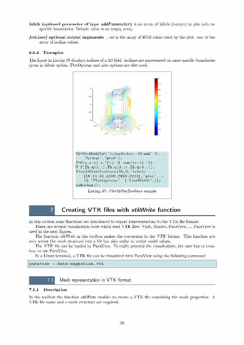
6.5.4 Examples
The gure in Listing 35 displays isolines of a 3D eld. Isolines are represented on some specic boundariesgiven in labels option. PlotOptions and niso options are also used.
Th=GetMeshOpt ( ' cy l inderkey ´10.msh ' ,3 , ...' format ' , ' gmsh ' ) ;
f=@(x , y , z ) x.^2+y.^2+cos ( ( z´1) .^2) ;U=f (Th . q ( 1 , : ) ,Th . q ( 2 , : ) ,Th . q ( 3 , : ) ) ;P l o t 3DSur f I s o l i n e s (Th,U, ' l a b e l s ' , ...
[ 10 , 11 , 31 , 2000 , 2020 , 2021 ] , ' n i s o ' , ...15 , ' PlotOptions ' , ' LineWidth ' ,1)
colorbar ( ) ;
Listing 37: Plot3DSurfIsolines sample
7 Creating VTK les with vtkWrite function
In this section some functions are introduced to export representations to the VTK le format.There are several visualization tools which read VTK les: VisIt, Mayavi, ParaView, ... ParaView is
used in the next gures.The function vtkWrite in the toolbox makes the conversion to the VTK format. This function not
only writes the mesh structure into a le but also scalar or vector nodal values.The VTK le can be loaded by ParaView. To really proceed the visualization, the user has to know
how to use ParaView.In a Linux terminal, a VTK le can be visualized with ParaView using the following command
paraview --data=magnetism.vtk
7.1 Mesh representation in VTK format
7.1.1 Description
In the toolbox the function vtkWrite enables to create a VTK le containing the mesh properties. AVTK le name and a mesh structure are required.
25
7.1.2 Usage
• Basic usage
Th=GetMeshOpt ( . . . ) ;vtkWrite ( cFileName ,Th) ;
7.1.3 Arguments
cFileName (input parameter) is a string for the VTK le name (with .vtk extension)
Th (input parameter) is a mesh structure (see 4.2)
No output argument
7.1.4 Examples
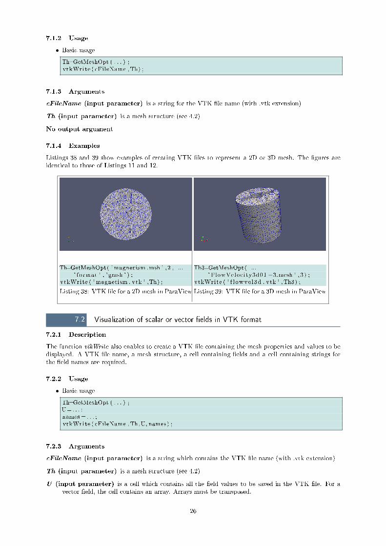
Listings 38 and 39 show examples of creating VTK les to represent a 2D or 3D mesh. The gures areidentical to those of Listings 11 and 12.
Th=GetMeshOpt ( 'magnetism .msh ' ,2 , ...' format ' , ' gmsh ' ) ;
vtkWrite ( 'magnetism . vtk ' ,Th) ;
Listing 38: VTK le for a 2D mesh in ParaView
Th3=GetMeshOpt ( ...' FlowVelocity3d01 ´3.mesh ' , 3 ) ;
vtkWrite ( ' f l owve l3d . vtk ' ,Th3) ;
Listing 39: VTK le for a 3D mesh in ParaView
7.2 Visualization of scalar or vector elds in VTK format
7.2.1 Description
The function vtkWrite also enables to create a VTK le containing the mesh properties and values to bedisplayed. A VTK le name, a mesh structure, a cell containing elds and a cell containing strings forthe eld names are required.
7.2.2 Usage
• Basic usage
Th=GetMeshOpt ( . . . ) ;U= . . . ;names = . . . ;vtkWrite ( cFileName ,Th,U, names ) ;
7.2.3 Arguments
cFileName (input parameter) is a string which contains the VTK le name (with .vtk extension)
Th (input parameter) is a mesh structure (see 4.2)
U (input parameter) is a cell which contains all the eld values to be saved in the VTK le. For avector eld, the cell contains an array. Arrays must be transposed.
26

names (input parameter) is a cell variable which contains the names of the eld values
No output argument
7.2.4 Examples
Listings 40 and 41 are examples of creation of VTK le containing mesh properties and scalar values.There are two scalar values in the 3D example. Listing 42 shows an example of VTK le showing themagnitude of a vector variable. Listing 43 is an example of VTK le showing the Y-component of avector variable with streamlines.
Th=GetMeshOpt ( 'magnetism .msh ' ,2 , ...' format ' , ' gmsh ' ) ;
U=2+cos (pi ∗(Th . q ( 1 , : ) .^2+Th . q ( 2 , : ) .^2) ) ;vtkWrite ( 'magnetism´s . vtk ' ,Th, ...
U' , 'u ' ) ;
Listing 40: VTK/2D scalar results
Th3=GetMeshOpt ( ' sphere8 ´4.msh ' ,3 , ...' format ' , ' gmsh ' ) ;
U=cos (Th3 . q ( 1 , : ) .^2+ ...Th3 . q ( 2 , : ) .^2+Th3 . q ( 3 , : ) .^2) ;
V=cos (Th3 . q ( 1 , : ) .^2+ ...Th3 . q ( 2 , : ) .^2+Th3 . q ( 3 , : ) .^2) ;
vtkWrite ( ' sphere8´4 s . vtk ' ,Th3 , ...U' ,V' , 'u ' , ' v ' ) ;
Listing 41: VTK/3D scalar results
27
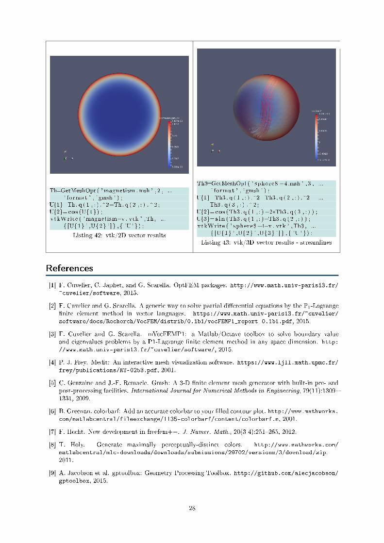
Th=GetMeshOpt ( 'magnetism .msh ' ,2 , ...' format ' , ' gmsh ' ) ;
U1=Th . q ( 1 , : ) .^2+Th . q ( 2 , : ) . ^ 2 ;U2=cos (U1) ;vtkWrite ( 'magnetism´v . vtk ' ,Th, ...
[U1 ' ,U2 ' ] , 'U ' ) ;
Listing 42: vtk/2D vector results
Th3=GetMeshOpt ( ' sphere8 ´4.msh ' ,3 , ...' format ' , ' gmsh ' ) ;
U1=Th3 . q ( 1 , : ) .^2+Th3 . q ( 2 , : ) .^2+ ...Th3 . q ( 3 , : ) . ^ 2 ;
U2=cos (Th3 . q ( 1 , : )´2∗Th3 . q ( 3 , : ) ) ;U3=sin (Th3 . q ( 1 , : )+Th3 . q ( 2 , : ) ) ;vtkWrite ( ' sphere8´4 v . vtk ' ,Th3 , ...
[U1 ' ,U2 ' ,U3 ' ] , 'U ' ) ;
Listing 43: vtk/3D vector results - streamlines
References
[1] F. Cuvelier, C. Japhet, and G. Scarella. OptFEM packages. http://www.math.univ-paris13.fr/~cuvelier/software, 2015.
[2] F. Cuvelier and G. Scarella. A generic way to solve partial dierential equations by the P1-Lagrangenite element method in vector languages. https://www.math.univ-paris13.fr/~cuvelier/
software/docs/Recherch/VecFEM/distrib/0.1b1/vecFEMP1_report-0.1b1.pdf, 2015.
[3] F. Cuvelier and G. Scarella. mVecFEMP1: a Matlab/Octave toolbox to solve boundary valueand eigenvalues problems by a P1-Lagrange nite element method in any space dimension. http:
//www.math.univ-paris13.fr/~cuvelier/software/, 2015.
[4] P. J. Frey. Medit: An interactive mesh visualization software. https://www.ljll.math.upmc.fr/frey/publications/RT-0253.pdf, 2001.
[5] C. Geuzaine and J.-F. Remacle. Gmsh: A 3-D nite element mesh generator with built-in pre- andpost-processing facilities. International Journal for Numerical Methods in Engineering, 79(11):13091331, 2009.
[6] B. Greenan. colorbarf: Add an accurate colorbar to your lled contour plot. http://www.mathworks.com/matlabcentral/fileexchange/1135-colorbarf/content/colorbarf.m, 2001.
[7] F. Hecht. New development in freefem++. J. Numer. Math., 20(3-4):251265, 2012.
[8] T. Holy. Generate maximally perceptually-distinct colors. http://www.mathworks.com/
matlabcentral/mlc-downloads/downloads/submissions/29702/versions/3/download/zip,2011.
[9] A. Jacobson et al. gptoolbox: Geometry Processing Toolbox. http://github.com/alecjacobson/gptoolbox, 2015.
28

[10] J. R. Shewchuk. Triangle: Engineering a 2D Quality Mesh Generator and Delaunay Triangulator. InMing C. Lin and Dinesh Manocha, editors, Applied Computational Geometry: Towards GeometricEngineering, volume 1148 of Lecture Notes in Computer Science, pages 203222. Springer-Verlag,1996.
Warning GIT! Working tree is dirty!!GIT commit abab91016db01eb54bf8bb0a19d144179c79a722Date: Sun Feb 12 23:34:55 2017 +0100
29