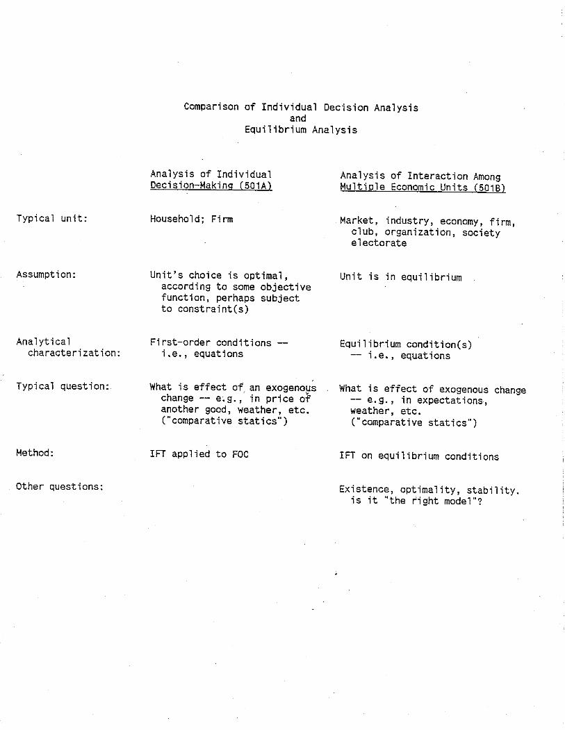
The Definition of Market Equilibrium

The concept of market equilibrium, like the notion of equilibrium in just about every other

context, is supposed to capture the idea of a state of the system in which there are no forces

tending to cause the state to change to a different state. For a market system, we think some

prices are likely to change if there is excess demand or supply for any of the goods; and conversely

that if all markets clear — i.e., if no good is in excess demand or supply — then the prices will not

change. And since the quantities that are transacted depend on the prices, the quantities should

not change, either. So the natural definition of a general equilibrium of all markets is that all the

markets clear — i.e., that the price-list p ∈ Rl+ satisfies the equilibrium condition

∆

X (p) = 0 i.e.,∆

Xk (p) = 0 , k = 1, . . . , l. (∗)

Provisional Definition: Let E = ((ui, x̊i))ni=1 be an economy consisting of n consumers (ui, x̊i).

Let xi(·) : Rl+ → Rl denote the demand function of consumer (ui, x̊i), and let

∆

X (·) : Rl+ → Rl

denote the market net demand function∆

X (p) :=∑n

i=1(xi (p)− x̊i). A market equilibrium of

E is a price-list p ∈ Rl+ that satisfies the equilibrium condition (∗).

There are many situations where this definition works just fine, but there are also many situations

where it’s not satisfactory. For example,

(1) If a price pk is zero and there is excess supply of good k — i.e.,∆

Xk (p) < 0 — it seems unlikely

that this would lead to a change in any of the prices.

(2) What if the demand function xi(·) is not well-defined at some price-lists p for one or more

consumers (ui, x̊i)? For example, if pk = 0, the CMP for some consumers may not have a solution.

(3) What if some consumer’s demand function xi(·) is not single-valued at some price-lists? For

example, a utility function ui might have an indifference curve with a “flat spot” — an extreme

example is a linear utility function u(x, y) = ax + by.

The following definition explicitly avoids issues (2) and (3) by including only situations in which

all demand functions are well-defined and single-valued for every price-list p ∈ Rl+. The defini-

tion takes account of issue (1) by allowing that excess supply of some goods is consistent with

equilibrium if those goods have a price of zero.

Definition: Let E = ((ui, x̊i))ni=1 be an economy consisting of n consumers, all of whose demand

functions xi(·) : Rl+ → Rl are well-defined and single-valued on Rl

+, and let∆

X (·) : Rl+ → Rl denote

the corresponding market net demand function. A market equilibrium of E is a price-list p ∈ Rl+

that satisfies the equilibrium condition

∀k = 1, . . . , l :∆

Xk (p) 5 0 and∆

Xk (p) = 0 if pk > 0. (Clr)

We’ll also refer to a price-list that satisfies (Clr) as an equilibrium of the net demand function∆

X (·).

We’ll use this equilibrium condition throughout the course, so we give it a name that we’ll use

to refer to it: (Clr), which is an abbreviation for Clear, since the condition says that all markets

clear.

A market equilibrium is also called a Walrasian equilibrium. An essential feature of this equilib-

rium concept is the assumption — implicit in the definition — that all consumers are price takers.

Each consumer, in solving his consumer maximization problem, treats the prices as parameters

that will be unaffected by his decision about which consumption bundle he will choose.

Some Remarks

(1) Note the analogy with optimization: Here the equilibrium conditions are equations that deter-

mine the values of the variables, and in optimization the first-order conditions are equations that

determine the values of the variables.

(2) With l goods we will have l − 1 independent equilibrium conditions (equations), with Wal-

ras’s Law accounting for the remaining market, so only l − 1 relative prices are determined by

equilibrium. (We could, for example, use one of the prices as “numeraire.”) Because the demand

functions are homogeneous of degree zero, they also depend only on the relative prices.

(3) What if, unlike in our Cobb-Douglas examples, we can’t get a closed-form solution (i.e., an

explicit expression) for the state variables in terms of the parameters? How do we do comparative

statics in that case? We can apply the Implicit Function Theorem to the equilibrium equations,

just as we apply the IFT to the first-order equations to do comparative statics for optimization.

(4) The approach in (3) is often not good enough: for example, we often need to determine the

actual equilibrium prices and/or quantities, not just the comparative statics derivatives. If we can’t

get closed-form solutions (which is the typical situation), we can try to compute the equilibrium

values. How do we do that?

(5) What if there is no equilibrium? Under what conditions will there be an equilibrium?

(6) What if there are multiple equilibria? Under what conditions will there be a unique equilibrium?

(7) What if the system is not in equilibrium? What are the stability properties of the equilibrium?

(8) Is the equilibrium outcome a good outcome?

(9) What if markets and prices aren’t used? Under what conditions will they be used?

(10) What if not everyone is a price-taker?

We will address all of these questions in the course, some in depth, and others only in passing.