INSTITUT NATIONAL DE LA STATISTIQUE ET DES ETUDES ECONOMIQUES Série des Documents de Travail du CREST

(Centre de Recherche en Economie et Statistique)

n° 2008-12

The Effect of Widowhood on Housing and Location Choices

C. BONNET1 L. GOBILLON2

A. LAFERRÈRE3 Les documents de travail ne reflètent pas la position de l'INSEE et n'engagent que leurs auteurs. Working papers do not reflect the position of INSEE but only the views of the authors.

1 INED, 133 boulevard Davout, 45980 Paris Cédex 20. Tel. : 33 (0) 1 56 06 22 36. carole.bonnet@ined.fr 2 INED. Tel. : 33 (0)1 56 06 20 16. laurent.gobillon@ined.fr 3 INSEE and CREST, 18 boulevard Adophe Pinard, 75675 Paris Cedex 14. Tel. : 33 (0) 1 41 17 55 74. anne.laferrere@insee.fr

L’effet du veuvage sur les choix de logement et de localisation

Carole Bonnet, Laurent Gobillon et Anne Laferrère

Résumé Le nombre de veuves augmente avec le vieillissement de la population, et leur influence sur le marché

du logement risque de s’accroître. Cet article s’intéresse à l’effet du veuvage sur les choix de logement

et de localisation. Le décès d’un partenaire a pour effet de diminuer le revenu, ce qui peut conduire à

diminuer sa consommation de logement. Le veuvage peut aussi révéler de nouvelles préférences, par

exemple le besoin d’habiter près d’un pourvoyeur de soins, ou de services de santé. Nous estimons

l’effet d’une transition vers le veuvage sur la consommation de logement à partir des enquêtes

nationales sur le Logement. Le veuvage augmente significativement la mobilité résidentielle,

spécialement aux âges élevés, et si on a des enfants. Les veufs ou veuves récents on tendance à choisir

de vivre plus près de leurs enfants, mais pas à habiter sous le même toit qu’eux. Les ajustements de

logement et de localisation sont compatibles avec un modèle où le veuvage fait bouger vers un

logement plus petit, plus fréquemment un appartement, en secteur locatif, et en moyenne localisé dans

une commune plus grande où les services sont plus facilement accessibles.

The effect of widowhood on housing and location choices

Abstract

The number of widows has been increasing with population ageing and their influence on the housing

market is getting larger. This paper investigates the effect of widowhood on housing and location

choices. A partner's death induces a decrease in income which may lead to downsizing. Widowhood

may also reveal new preferences, such as the need to be close to care givers and health services. We

estimate the effect of a transition to widowhood on housing consumption and location choices using

the French Housing Surveys. Widowhood significantly increases residential mobility, especially at

older ages and when having children. Mobile recent widows tend to live closer to their relatives but do

not move to co-reside with a child. Housing and location adjustments are consistent with new widows

moving to dwellings that are smaller, more often apartments and in the rental sector, and on average

located in larger cities where services are more accessible.

1 Introduction

As the population is ageing, governments are concerned with the �nancing of pensions, as well

as the costs of health and care services. In this context, widowhood is getting important with

the arrival of large baby-boom cohorts at the age of widowhood (Kalogirou and Murphy, 2006).

Widowhood a¤ects welfare in many ways. It a¤ects income and living standards as the survivor�s

pension is smaller than the partner�s income. Housing accounts for an important share of the

budget and its consumption presents economies of scales that are lost when the partner dies. For

this reason a surviving spouse may want to downsize. Widowhood also a¤ects living arrangements.

It is well documented that a fair amount of care to disabled elderly people is provided by a spouse,

who is most often the wife (Chappell, 1991, Freedman, 1996). Obviously a widow has no care-

providing spouse in case of need. She has to turn to other family members or to professionals

�nanced by private or public insurance. The issue of long term care is linked to the housing

choices of the oldest old, as they choose between accommodation in nursing homes or personal

care in their own dwelling. As the number of widows is expected to increase in the near future,

the consequences on the housing market may be important. We study the residential mobility,

housing and location choices of recent widows and widowers. Do they downsize? Do they relocate?

Our goal is to get some indirect evidence on the impact of the residential mobility of widows on

the housing market and to what extent widows may rely on kinship for support.

Quite surprisingly, the mobility and housing choices of the elderly have not often been analyzed

in the economic literature except in a few empirical papers (Venti and Wise, 1989; Ermisch and

Jenkins, 1999; Venti and Wise, 2001; Tatsiramos, 2004; Laferrère, 2005 and 2006). These studies

adopt a broad view, looking at the e¤ect of all shocks - job change, retirement, widowhood -

on mobility. They also analyze the variations in housing characteristics and location as a move

occurs. However, they do not usually disentangle the various causes of mobility. Hence, the

results are generated by a mix of several economic and socio-demographic e¤ects. Conversely, the

literature on widowhood does not look much at mobility (with the exception of Chevan, 1995)

and housing choices. It mostly studies the living arrangement of widows at a given point in time

and not its dynamics (Macunovich et al., 1995, Costa, 1999, Iacovou, 2000). The present paper

tries to reconcile the two approaches and explain how widowhood can lead to mobility, housing

1

adjustments and relocation.

We propose a two-period model to show how the changes in income and preferences due to wid-

owhood may a¤ect housing and location choices. In fact, when a partner dies, the loss of income

is only partly compensated by a survivor pension, while the housing cost per capita doubles. This

encourages downsizing. Besides, as a widow cannot bene�t from the help of a partner, she may

anticipate the need to get a better access to care especially at an older age. This can be done by

getting closer to her children or to places where services are easily available such as large cities.

We assess the importance of these mechanisms in an empirical section using data from the French

Housing Surveys.

We �nd that a transition to widowhood has a signi�cant positive impact on residential mobility,

especially at older ages. Ceteris paribus, when one of the spouses dies, the probability of moving

within the next four years is nearly 90% higher than if no death occurred. A widow is more likely

to be mobile if she has children than if she is childless. Mobile widows tend to live closer to their

relatives even if moves to co-reside with a child are extremely rare. Compared to mobile couples,

mobile recent widows are more likely to decrease their number of rooms and to choose the rental

sector. They also switch more often from a single family house to an apartment. Finally they move

more often to larger cities. These results on housing and location adjustments are consistent with

moves to get closer to health services and care for single elderly people.

Section 2 provides descriptive statistics and discusses some institutional features of widowhood in

France. In section 3, we present the two-period model that analyzes the e¤ect of a transition to

widowhood on housing and location choices. We then test some of the mechanisms on data from

the 1996 and 2002 French Housing Surveys, which are described in section 4. Section 5 delineates

our empirical �ndings. Section 6 concludes.

2 The French setting

We now present some stylized facts on widowhood after age 60. Figure 1 shows the proportion

of widows and widowers by age, for �ve birth cohorts. The proportion increases with age, and is

always much larger for women than for men. The di¤erence can be explained by the higher death

rate of men and by the age di¤erence between spouses, as wives are on average 2:5 years younger

2

than their husbands. For instance, for women born in 1920, the rate of widowhood at age 80 is

60 percent, more than 3 times the rate for men (17 percent). This means that a large majority of

married men live with their spouses until death whereas a large majority of women spend part of

their life as widows. This justi�es our use of the word �widow� instead of �widow or widower� in

this paper. At a younger age, the rate of widowhood also decreases from one cohort to the other.

This is due to the general increase in life expectancy which makes widowhood occur later in the

life-cycle.1

[Insert F igure 1]

The death of a spouse induces a fall in the household resources as it goes with the loss of the

partner�s income. To compensate for this loss, widows in many countries are eligible for social

security bene�ts in the form of a survivor pension (see Burkhauser and alii, 2005). In France the

average survivor pension is roughly 55 percent of the deceased spouse�s pension. Hence, in many

cases, the survivor pension would not fully compensate for the income loss related to widowhood.2

It is not possible to compute the change in income due to widowhood using the French Housing

Surveys. Nevertheless, we can recover some indirect information from the average income of

cohorts as a function of the age of the household head (see Figure 2).

[Insert F igure 2]

A striking fact is that the average income does not decrease after age 70. This is surprising at a

�rst glance because many couples experience the death of one partner at that age (see Figure 1).

This income stability may be generated by three main mechanisms:

� First, as we mentioned above, the surviving spouse gets a survivor pension that is designed1Deaths among non legally married couples are not recorded as widowhood. The bias in negligible for the

current cohorts aged 60 or more. But for the future generations where lasting partnerships exist outside marriages,

a new word may have to be found for widowhood.2Suppose for example that the husband receives a pension PH and the wife has no pension. After the husband�s

death, the survivor pension will be 55 percent of PH . With the most commonly used equivalence scale, the living

standard of the surviving spouse will decrease from 0; 7PH (ie. PHp2 ) to 0; 55 PH ; that is to say by about 21%. If we

assume that the woman received PF equal to one third of PH , the decrease in the living standard will be roughly

10%.

3

to help him/her keep the same living standards. This survivor pension may be complemented

with the extraction of income from assets after the partner�s death.

� Second, mortality rates at older ages vary with education and income level. The life ex-pectancy of the lowest income groups is lower and on average they die �rst (Jusot, 2004).

Hence, there is a selection e¤ect as the proportion of high income households increases with

age.

� Third, some poor widows may move to sheltered housing or nursing homes. They are ex-cluded from our sample.3 Delbès and Gaymu (2005) �nd that entry in retirement home is

more likely for low-income groups.

Actually, living in an institution is rare below age 80, and so is co-residing with children (Flipo, Le

Blanc and Laferrère, 1999). Widows aged between 60 and 85 years old mainly live independently

(see Figure 3). Above 85, entries into nursing homes increase quickly. Nearly one third of widows

between 90 and 94 years old are institutionalized (Delbès and Gaymu, 2005).

[Insert F igure 3]

Widowhood can also in�uence a surviving spouse�s wealth because of the rules governing marriage

property and inheritance. Under the French marriage law,4 all assets acquired during marriage

are held in common, that is, half of them belong to each spouse. Hence after a death, half of the

couple�s common property belongs to the surviving spouse, but the other half is transmitted by

bequest. In the presence of children, a surviving spouse is not the only one to inherit her partner�s

property, as the children also inherit the property. Consequently, a surviving spouse may have to

share with her children the property of the dwelling that she used with her husband. Usually, the

transfer of ownership rights to the children does not change much for the widowed mother who can

go on using her home. But depending on the overall size of the bequest, she can be forced out of

her home. Typically if the couple�s only asset was the home, the children might put some pressure

3More precisely, only part of retirement homes and dwellings for the elderly are categorized as ordinary homes

and included in the French Housing Surveys used for Figure 2. These are mainly dwellings for non-disabled elderly.4As was applied until 2001. The law is now more favorable to the surviving spouse. See Laferrère (2001) for

more details on French marriage contracts, and Arrondel and Laferrère (2001) on inheritance rules.

4

on their surviving parent to sell the home and divide the money among the heirs, if only to pay

inheritance tax. Besides, an altruistic surviving mother may agree to sell the dwelling to help

her liquidity constrained children. This awkward state of a¤air can be prevented if the deceased

spouse has made a will which gives the surviving spouse a formal life interest in the home (the

usufruct) as long as she lives.5 Due to this feature of the French law, we expect that the more

children a widow has, the more likely she is to move from her home.

3 A theoretical model

3.1 The e¤ect of widowhood on housing choices

Leaving aside the issue of inheritance sharing, we propose a very simple two-period model to

illustrate how various factors may a¤ect mobility, housing and location choices after the death

of a spouse. In the �rst period, two identical retired individuals live together and choose their

consumption of a composite good and housing. At the end of the period, one partner (say the

husband) dies. In the second period, the widow chooses between two options: staying and mov-

ing. If she stays, she cannot adjust her housing consumption. If she moves, she can make such

adjustments but she incurs a moving cost. We analyze the trade-o¤s determining her choices.

Each spouse�s utility function U depends on the �ow of services derived from housing F and on

the consumption of a composite good C chosen as a numeraire: U = U (C;F ). A uni-dimensional

index K summarizes all the features of housing related to quality and quantity. For simplicity, we

label it housing quantity. The �ow of housing services is denoted �c (K), where the subscript c

stands for life in couple. The �ow is an increasing function of the quantity index. This function also

accounts for many characteristics of housing consumption as explained in Nelson (1988). Firstly,

it captures economies of scale in consumption, as housing is a partially public good. Secondly,

there can be increasing returns in the household production of goods and services. For instance,

cooking for two takes less than twice the time of cooking for one.6 Thirdly, there can be some

5For a dwelling, the usufruct is the right to use it. For a �nancial asset or a housing investment, it is its return.

Since 2001, the survivor has a life interest in the deceased spouse�s property even in the absence of a will.6Another type of scale economies mentioned by Nelson (1988) are scale economies in price. They exist when

the marginal cost of dwelling is a decreasing function of its quantity. In our framework (as in Nelson, 1988 from

5

positive complementarity e¤ects from sharing a home. One may enjoy watching television with a

partner more than alone. Moreover, some tasks, like gardening, may be performed better by one

of the spouses rather than the other one.

The utility function can be rewritten: Uc (C;K) = U (C; �c (K)). The function Uc is supposed to

be increasing in its two arguments and strictly concave. The additional assumption that @2Uc@C@K

> 0will be used in comparative statics. It is veri�ed for usual utility functions such as Cobb-Douglas

and CES, as well as for separable utility functions. We also assume that Uc veri�es the Inada

conditions to get an interior solution.

In the �rst period, each spouse gets a retirement pension I that is used to consume C in composite

good and to pay for housing. Housing consumption is characterized by a non negative housing

cost �. For owners, the user cost includes the opportunity cost of money invested in the house

and the maintenance costs (see Henderson and Ioannides, 1983). For tenants it is the rent.7 The

couple chooses a dwelling without fully anticipating the death of one partner. For simplicity, there

is no transaction cost in period 1. The two partners have the same bargaining power so that their

respective levels of welfare count equally in the household�s choices. We also assume that they

share equally the composite good. The maximization program of the couple is then:

maxC;K

2Uc (C;K) (1)

slc : 2C + �K = 2I

Rewriting the budget constraint as C + �2K = I, we can see that the program gives the same

optimal quantities as for a single individual with utility Uc endowed with income I and facing a

housing cost twice lower than the couple�s cost. We denote the optimum housing capital: Kc =

Kc

��2; I�where the �rst argument is the housing cost per capita and the second is income.

At the end of the �rst period, the husband dies. His widow receives a survivor pension R(I)

indexed on her husband�s retirement pension. The housing cost per capita doubles taking the

which it is very close), scale economies in price are formally equivalent to scale economies in consumption. We do

not insist on them as they remain the same when one partner dies. By contrast, scale economies in consumption

disappear.7Owners may get a positive return from housing if the housing prices increase enough: � < 0. In that case,

housing should be thought of as an asset entering a portfolio (see Bruekner, 1997; Flavin and Yamashita, 2002).

This case is not taken into account here as we focus only on mechanisms related to a transition to widowhood.

6

value �. The housing service �ow changes. The new service �ow function is denoted �w (K) where

the subscript w stands for widowed. It is still an increasing function of the housing quantity

index. There are several reasons why � may change after widowhood. On the one hand, possible

congestion disappears. Extra rooms may also yield additional bene�ts if the widow needs visitors

to overcome loneliness. These mechanisms have a positive e¤ect on the service �ow for a given

housing quantity. On the other hand, complementarity e¤ects with the partner, scale economies

in consumption, and increasing return in housing production disappear. These have a negative

e¤ect on the service �ow for a given housing quantity. We conjecture that, overall, negative e¤ects

usually prevail. We thus assume that the marginal rate of substitution MRS between housing

and the composite good is reduced after widowhood: MRSw < MRSc.

In the second period, the widow chooses between staying in the dwelling and moving. If she stays,

she cannot adjust her housing consumption to her new preferences and constraints. If she moves,

she can make such adjustments but she incurs a moving cost D. This cost includes monetary

costs like transportation or brokers�fees. It also includes the utility decrease, assumed to have a

monetary equivalent, arising from the loss of a local social network, the loss of local information,

and the pain of leaving a familiar environment.

We denote by Uw (C;K) = U (C; �w (K)) the widow�s utility function with the same standard

assumptions as for Uc. The widow maximizes her utility under the budget constraint. We assume

that the user cost is the same as in the �rst period.8 The maximization program can be decomposed

in two stages. For each option, staying and moving, the widow computes her optimal utility. She

then chooses the option yielding the highest utility.9 If she stays, her housing consumption index

remains at Kc and her consumption of the composite good is given by the second-stage budget

constraint: C = I + R (I)� �Kc. This option is valid only if the widow can pay for the housing

cost with her new income: �Kc < I +R (I). In some cases, the survivor cannot bear the housing

cost anymore, so she has to move. This occurs when the income I + R (I) is between �Kc=2 and

�Kc. It is an important policy issue for the low income elderly. In case of ownership, the elderly

8The extension of the model to a change in user cost is straightwforward and yields additional price e¤ects.9For simplicity, we do not model the tenure choice as it has been studied extensively in the literature and is not

speci�c to widowhood. This tenure choice rests mainly on the relative user costs and utility bene�ts of ownership

and rental, as well as the existence of borrowing constraints (see Gobillon and Le Blanc, 2004, for a modelization

in a two-period framework similar to ours). We keep these mechanisms in mind for the empirical section.

7

may try to decrease the maintenance costs to avoid being income constrained. Evidence for the

US suggests that the elderly spend less money in maintenance costs than younger homeowners

(Davido¤, 2006). This type of mechanism is not included in our model but it could be taken into

account by assuming that the owner�s user cost is endogenous.

In case of a residential move, the maximisation program writes:

maxC;K

Uw (C;K) (2)

slc : C + �K = I +R (I)�D

The optimal housing quantity is denoted: Kw = Kw (�; I +R (I)�D).The moving decision follows a (s; S) rule when the moving cost is small enough and variations

in housing quantity can yield signi�cant changes in utility.10 In that case, there is an inaction

band around the housing consumption of the �rst period. If the optimal housing consumption of

the widow stands within this band, it is not worth adjusting housing because of moving costs.

If the optimal housing consumption stands outside the band, moving allows to make a housing

adjustment that more than compensates the moving cost.

We now focus on the change in the housing consumption index in case of mobility. The di¤erence

in optimal housing quantity between the two periods can be decomposed as follows:

Kw �Kc = [Kw �Kw (�; I +R (I))]| {z }moving cost e¤ect: <0

+ [Kw (�; I +R (I))�Kw (�; I)]| {z }survivor pension e¤ect: >0

(3)

+hKw (�; I)�Kw

��2; I�i

| {z }user cost e¤ect: <0

+hKw

��2; I��Kc

i| {z }preference e¤ect: <0

The signs of the e¤ects are easy to derive (see Appendix 1). First, there is a negative income

e¤ect due to moving costs. This e¤ect is usually larger for owners than for renters as their moving

costs are usually higher. These is also an impact of the decrease in resources from 2I to I +R (I)

that can be decomposed into two parts. There is a positive income e¤ect as the survivor pension

increases the income per head from I to I+R (I). There is also a negative price e¤ect arising from

10The (s; S) rule in not peculiar to housing and arises more generally when studying the consumption of durable

goods in the presence of �xed costs. Also, it is not speci�c to widowhood. For a more detailed analysis of this rule,

see Grossman and Laroque (1990), Martin (2003), Gobillon and Le Blanc (2004), Flavin and Nakagowa (2004).

8

the fact that the user cost of housing per head doubles from �2to �. The sum of these two e¤ects is

likely to be negative as income per head less than doubles whereas housing cost per head doubles.

Finally, the preference e¤ect is negative as the service �ow from housing decreases and housing

becomes less valuable after widowhood. The di¤erence Kw�Kc is likely to be in�uenced by other

factors not included in the model. First, couples may anticipate the death of one partner and

choose their home as a compromise between their optimal choice when living together as a couple

and when living alone. The model can be extended to integrate this feature in an inter-temporal

framework. The utility function in the �rst period would be a weighted sum of the utility of the

couple and the utility of a widow. In that case, housing adjustments in the second period are less

likely.11

The decomposition (3) and the analysis which goes along suggest that downsizing is likely. We

test it empirically below.

3.2 Location decision

So far, we have assumed that housing consumption could be summarized by a single index K.

However housing has many dimensions. A major aspect is location. Places di¤er in amenities such

as climate, or cultural goods. More importantly in our context, they di¤er in access to services.

When living together, the two partners choose a common location according to their preferences.

When one of them dies, the survivor may relocate according to her own new preferences and con-

straints. Among changes in preferences, an important aspect is closeness to friends and relatives,

as well as access to services and care providers. We now extend the model to jointly study the

housing and location adjustments.

Consider two locations a and b with di¤erent housing costs. In our context, a can be thought

of as a rural area or a small town, and b as a large city providing services and shops, or as the

place where the children live. For location ` 2 fa; bg, the housing cost is denoted � (`). In the�rst period, the couple chooses the consumption of housing and of the composite good, as well

as a location. Each partner�s utility depends on the location ` and writes U c (C;K; `). For a

11Also, partners may have di¤erent preferences and di¤erent bargaining power in the decisions taken within the

couple. Then, a transition to widowhood might reveal the individual�s own preferences and change the optimal

housing index in the second period.

9

�xed `, the utility function is strictly concave in (C;K) and veri�es the Inada conditions. The

maximization program can be decomposed in two stages. First, the couple computes its optimal

utility in each location `:

Vc (`) = maxC;K

2U c(C;K; `) (4)

slc : 2C + � (`)K = 2I

Then, the couple chooses the location `c yielding the highest utility. Without loss of generality,

we suppose that the location at optimum is a (the small town).

In the second period, the widow may stay in her dwelling or move depending on the welfare

provided by the two options. If she stays, she cannot adjust her housing quantity (see the previous

section). If she moves, she can choose both her location and housing quantity. For simplicity, we

suppose that the moving costs are the same whatever the location she chooses. Denote Uw (C;K; `)

the widow�s utility function in a given location `.12 For this location, the optimal utility is given

by:

Vw (`) = maxC;K

Uw (C;K; `) (5)

slc : C + � (`)K = I +R (I)�D

The optimal location when moving is the one yielding the highest utility.

In this setting, the transition to widowhood reveals the new individual preferences for housing and

location. The widow may relocate if her new preferences make her prefer b to a. The location b

could be closer to her family or could become more attractive because of better service accessibility.

Interestingly, the location choice itself may induce a decrease in the housing quantity. This happens

if the widow wants to relocate to a large city and the housing cost in the rural area is lower than

in the large city: � (a) < � (b).

Location is only one of many dimensions of housing. Other dimensions are the number of rooms,

equipment, and whether the dwelling is an apartment or a house. Besides, the local housing market

is di¤erent in a rural area and in a large city. There are usually more apartment buildings and less

single-family houses in cities, and dwellings are more often for rent. Hence, a new widow located

in a rural area who owns a house is likely to rent an apartment if she moves to a city. Note that

12For a �xed `, this function is supposed to be strictly concave in (C;K) and to verify the Inada conditions.

10

choosing to own may be less attractive as one ages, as one has less time to recover the cost of

investment. This would induce older movers, widowed or not, to choose to rent rather than own.

The empirical section will investigate the housing adjustments in location, size, dwelling type and

tenure status.

4 The data

Our theoretical model has several empirical implications for mobility and housing adjustments

after widowhood. To test them, we need information on residential and family history, as well

as on the characteristics of the former and current accommodation. Not many datasets provide

such information. Panel data would seem well adapted to study transitions. However their sample

size is small. For instance in the European Community Household Panel, only 65 males and 192

females became widowed over the 1994-2001 period (Ahn, 2004).13 Besides, panel attrition is

likely to be endogenous as mobile households are more di¢ cult to retrieve. For those reasons we

use the 1996 and 2002 French Housing Surveys (FHS) that o¤er large representative samples of

the population. These cross-section surveys are designed to study residential mobility. They o¤er

a large choice of retrospective questions on the housing situation four years before the survey date,

as well as questions on whether a move occurred within the last four years and the reasons for

this move. The data also include some information on the usual socio-demographic characteristics

of individuals and their detailed income. Importantly, the 2002 Housing survey also provides the

total number of children outside the parents�home, which is likely to be an important element of

preferences and constraints.

We de�ne a mobile household as one who changed homes within the last four years before the

survey date. We restrict the sample to households whose head is retired or inactive and was aged

between 60 and 85 four years before the survey date. The exclusion of those who are employed is

meant to decrease transitions on the labor market that can lead to residential mobility without any

13In the US Panel Study on Income Dynamics (1980-1997), the German Socio-Economic Panel (1984-2000),

the British Household Panel (1991-2000) and the Canadian Survey of Labour and Income Dynamics (1993-2000),

roughly 571, 345, 197 and 633 females aged 50 years old and over experience a transition to widowhood (Burkhauser

and alii, 2005).

11

link to widowhood.14 The exclusion of the oldest old is meant to minimize entries in nursing and

elderly homes that increase after age 80 but are not frequent before age 85 (Delbès and Gaymu,

2005, and Figure 3). We impose this exclusion because most of those living in institutions are

excluded from the sample.

The surveys provide no direct information on matrimonial status four years before the survey

date, but current status and the number of household members are known. Hence, a transition to

widowhood is de�ned in the following way: a person is widowed and lives alone at the survey date,

and the number of household members decreased from two to one during the four years before the

survey.

This de�nition ignores recently widowed moving to live with their children. However their number

is negligible and ignoring them does not induce any signi�cant bias (See Appendix 2). Neither

do we study widowhood when it occurs in a couple living with children. This type of transition

represents less than 10 percent of recent widowhood in 2002.

Our �nal sample consists of 14,257 households (6,610 in the 1996 FHS and 7,647 in the 2002 FHS)

among whom 1,016 individuals experience a transition to widowhood (441 in the 1996 FHS and

575 in the 2002 FHS).15 As mentioned above, the size of our sample is an attractive feature of the

FHS compared to some alternative panel datasets. Descriptive statistics are presented in Table

1.16

[Insert Table 1]

Table 2 gives the rates of transition to widowhood among couples for the 1996 and 2002 FHS.

They are increasing with age. Between 1998 and 2002, some 30 percent of couples aged 80-84

experienced the loss of a spouse. Note that widowhood is less frequent at earlier ages but is more

frequent at later ages in the 2002 FHS than in the 1996 FHS. As was noted for the cohort e¤ect in

Figure 1, these di¤erences are related to the fast increase in life expectancy that makes widowhood

14This exclusion does not avoid the e¤ect of retirement on mobility that would occur after retirement. However

only 8 mobile households gave this reason for their move in our sample (see Table 9).15In the 1996 FHS, 103 males and 338 females experience widowhood. In the 2002 FHS, the corresponding �gures

are 144 males and 431 females.16Also, the period covered by longitudinal surveys is often longer and behaviors may change over time.

12

happen later in the life cycle.

[Insert Table 2]

In what follows, the date of the survey (1996 or 2002) is labeled t and the date four years before

is labeled t� 1. We de�ne six non-overlapping types of family situations from marital status and

shocks on household composition:

(1) �Couples�: two people living together in t� 1, whether they are legally married or not17 andstill living together in t.

(2) �Single or divorced�: a person living alone in t� 1, and single or divorced in t.(3) �Widows�: a person living alone in t� 1, and widowed and living alone in t.(4) �3 people and more�: households with more than two members in t� 1.18

(5) �Recently widowed�: a person living with a partner as a couple in t � 1, and widowed andliving alone in t.

(6) �Recently separated�: a person living with a partner as a couple in t � 1, and divorced andliving alone in t.

Whereas couples are the largest group and account for 42 percent of the sample in 2002, stable

widows are the second largest group at 26 percent. The percentage of recently widowed is 8

percent.19 Table 3 gives the residential mobility rates for each of the six types. Leaving aside the

few who have recently divorced, recently widowed have the highest mobility rate. Indeed their

rate is 13:3 percent in 2002, more than twice the rate of couples. Interestingly, the mobility rate

of stable widows is also far smaller (7:9 percent) than when widowhood is recent. It suggests that

when widowhood induces mobility, it is mostly in the four years after the partner�s death.

[Insert Table 3]

17Most of the time, two people over 60 years old living together are married.18This group includes some couples with children who experience the death of one of the partners. We do not

distinguish them as we focus on transitions to widowhood for households with only two members.19We exclude the couples who recently separated in the rest of the analysis, as they represent only 1 percent of

our sample, which is too small to identify speci�c e¤ects for them.

13

5 Empirical results

5.1 Mobility

The theoretical section suggested several mechanisms which can make recently widowed more

mobile than couples. We now assess empirically the e¤ect of being recently widowed on mobility.

We estimate a probit model of mobility where the dependent variable is a dummy equal to one in

case of a move and zero otherwise. Di¤erences in mobility between family types are captured by

four dummies, each corresponding to one of the family categories (2)-(5) de�ned in the previous

section. Couples in category (1) are the reference. The theory suggests the importance of children

both as possible providers of care and help, and as possible claimants to the inheritance of the

parental home. We thus introduce a dummy for the existence of children living outside the parents�

home in our regressions.20 Beside the usual socio-demographic preferences shifters (age, sex and

education), we include housing and location variables. Housing tenure and housing type are used

as proxies for mobility costs, dwelling quality, and long term adequation to needs. The population

size of the municipality (less than 1,000 inhabitants; 1,000-5,000; 5,000-10,000; 10,000-50,000; and

more than 50,000) captures e¤ects related to the structure of the housing market.

Finally, the theory suggests that the income level after the partner�s death may a¤ect mobility.21

On the one hand, income can have a positive e¤ect as it helps to �nance moving costs. On the

other hand, it can have a negative e¤ect because low-income recently widowed may be unable to

pay for their housing expenditure and are then forced to downsize. The overall e¤ect on mobility

is an empirical issue and the theoretical arguments given above suggest that it may be non linear.

We �rst introduced income and its square in our probit regression. The e¤ect of income was found

to be inverse U-shaped with the vast majority of observed households being on the increasing

part of the parabola (the maximum of the parabola being as high as 86; 000 euros). Hence, the

20As the only FHS to provide information on the number of independent children is the one conducted in 2002,

we only use that survey.21Theory would suggest studying the e¤ect of the variation in income due to the partner�s death on the mobility

of recently widowed. However, we only have information on income at the survey date and not four years before.

We thus cannot compute the variation in income from the data. This means that the dummy for being recently

widowed will capture the e¤ect of the income variation on mobility.

14

income e¤ect is positive and nearly linear, and we stick to a linear speci�cation (in log). Income

after widowhood might be endogenous since new mobile widows may sell a dwelling, invest in a

�nancial asset and get some extra income. To overcome this di¢ culty, we instrument income after

widowhood with the overall pension of the recently widowed, that includes both her own pension

and the survivor pension. This pension is �xed by the law from the level of incomes of the two

partners before retirement and is thus exogenous. Table A in Appendix 3 reports the results of

the �rst-stage instrumental equation. Our �nal speci�cation is an IV probit.

Our �rst speci�cation tests for di¤erences in mobility between family categories (Table 4,

column 1). Single or divorced, as well as recently widowed, are found to be more mobile than

couples. In fact, recently widowed are the most mobile. Ceteris paribus, their probability of

moving is nearly 90% higher than for couples. Note that those who have been widowed for more

than four years have a propensity to move similar to couples. This suggests that if a move occurs

because of widowhood, it is likely to happen just after the death of the partner. This result is in

line with that obtained on the US Panel Study of Income Dynamics (Chevan, 1995).

Mobility is also found to be decreasing with age, except at older ages where it levels o¤.

Education has no signi�cant e¤ect. This is not surprising since residential mobility related to the

education choices would have occurred sooner in the life-cycle. The positive e¤ect of income on

mobility is in line with the need to pay for moving costs but not with liquidity constraints that

would force a move to reduce housing costs. Note that income is only weakly endogenous since

all coe¢ cients are very similar whether instrumenting or not (see the results of a simple probit in

Table B in Appendix 3 for comparison). Interestingly, those who have children are signi�cantly

more mobile than those who are childless. This result is consistent with a story where parents

would relocate closer to their children either to get some support (Ogg and Renaut, 2005, Glaser

and Tomassini, 2000, Laditka and Laditka, 2001) or to take care of their grand-children. The e¤ect

of tenure is also in line with expectations. Owners are less mobile than tenants, probably because

they have to incur large transaction costs and because ownership allows to better customize the

occupied dwelling. We also �nd the usual result for France that private-sector tenants are more

mobile than public housing tenants (Gobillon, 2001). Indeed, public housing tenants pay rents

that are lower than in the private sector and would loose this bene�t when moving. Living in a

single family house has a negative e¤ect on mobility, probably because it usually goes along with

15

higher quality. There is also a positive e¤ect of living in a large municipality (more than 50; 000

inhabitants) on mobility, maybe because it makes easier to �nd an accommodation more adapted

to new needs close to the previous dwelling. Finally the number of excess rooms, de�ned as the

number of rooms minus the number of persons, has no signi�cant e¤ect on mobility.

To shed more light on the speci�c behavior and constraints of the newly widowed, we then run

separate probits for three di¤erent family categories: couples, stable and single widows, and newly

widowed (Table 4, columns 2 to 4). Interestingly, the age pro�le and the e¤ect of children are

very di¤erent for the recently widowed. Recently widowed are more mobile when they get above

80, contrary to couples and stable widows. This is consistent with housing adjustments triggered

by health problems after the age of 80. While someone living in couple can rely on a spouse for

care and stay at home, an older widow may have to move to get care. She may want to relocate

closer to her children or to a place where health services and medical care are more accessible.

Having children has a positive e¤ect on the propensity to move (signi�cant at 10%) only for

recently widowed, and has no e¤ect for couples and stable widows. It is hard to disentangle the

reasons for this positive e¤ect: it may point to the need for family support at close range, or to

some pressure by children at the time of inheritance. Indeed, some of the moves may be due to the

necessity of sharing the deceased parent�s bequest. The pressure is likely to be more important for

widows than for widowers because the women of the cohorts we studied might own fewer personal

assets than their husbands. Consistent with this idea, we �nd that widows are more likely to

move than widowers. A more convincing test would be to interact the children dummy with the

sex dummy. Unfortunately the sample has not enough recent childless widowers to get convincing

results. Females are more a¤ected by disabilities than males of the same age (Cambois et al.,

2003). The signi�cant positive e¤ect of the female dummy is thus also compatible with their

having, or anticipating, more health problems.

The number of excess rooms has a positive e¤ect for widows but not for couples. This may be

a sign of the �nancial burden of a large dwelling. The next subsection analyzes the housing choices

of movers and will bring some additional elements pointing at widows being income constrained.

[Insert Table 4]

16

5.2 Housing choices of mobile widows

The theoretical model shows that recent widowhood can lead to an adjustment in housing con-

sumption and possible downsizing. A means to downsize is to reduce the number of rooms. To get

a large enough sample of movers, we now use both the 1996 and 2002 surveys. While 30 percent of

moving couples increase the number of rooms, 39 percent decrease it. By contrast, only 9 percent

of mobile recent widows increase their number of rooms, while 74 percent decrease it. Moreover,

half of those who downsize do it by two rooms or more. To get more insight into the determinants

of downsizing, we estimate a multinomial logit model where the dependant variable takes three

values: no change in the number of rooms (reference), an increase, or a decrease. Explanatory

variables remain the same as in the last section, except for the number of children outside home

which is excluded since it is not available in the 1996 Survey. Results are reported in Table 5.

Conditionally on moving, the number of excess rooms has a positive e¤ect on downsizing and a

negative e¤ect on upsizing. Hence, the disequilibrium in number of rooms tends to be corrected

by the move.22 More income induces upsizing (signi�cant at 10%). This might be a hint that

the wealthiest are less forced into decreasing their housing consumption because of a budget con-

straint. Whereas mobile recent widows are more likely to downsize than moving couples, there is

no signi�cant di¤erence for upsizing. This result is consistent with our theoretical expectations.

[Insert Table 5]

We also examine the change in the dwelling type (apartment/house) for moving households. The

proportion of recent widows living in an apartment doubles after a move. Whereas only 36 percent

of them lived in an apartment four years before the survey date (i.e. before the move), they are

73 percent at the survey date (i.e. after the move). By comparison, the increase is negligible

for couples: 45 percent of them live in an apartment before the move and 47 percent after the

move. We check that this result still holds when controlling for our set of explanatory variables.

We de�ne two subsamples depending on the dwelling type (apartment or house) before the move.

For each subsample, we estimate a logit model of housing type after the move (i.e. at the survey

date). Results are reported in Table 6. As expected, among house occupiers, recently widowed are

more likely to get into an apartment than couples. So are stable widows, as well as single and

22This �nding is similar to that obtained for retiring French households by Gobillon and Wol¤ (2007).

17

divorced individuals. Moves towards apartments signi�cantly increase with age until 80. This is

not surprising as living in a house usually goes along with more costs and maintenance tasks to be

performed individually, while they are taken care of collectively in apartment buildings. As one

ages, such tasks become more di¢ cult to perform. Also, single family houses in France are mostly

located far from town centers where shops and health services are usually located. Moving from a

house to an apartment may grant the elderly living on their own better access to these services.

[Insert Table 6]

In the same line, we investigate the e¤ect of being widowed on a change in housing tenure for

movers. Among moving owners, we expect recent widows to switch more often to the rental sector

than couples as owning is harder to deal with for a single person because of maintenance tasks

and paperwork. Indeed, among recent widows, 51 percent of owners switch to renting when they

move. Conversely, only 18 percent of renters switch to owning. The proportions for couples are

respectively 19 percent and 29 percent. As previously, we test whether our results are robust when

controlling for our set of explanatory variables. For each tenure mode before the move (renting

or owning), we estimate a logit model of housing tenure after the move. The results con�rm that

widows, whether recent or not, switch more often from owning to renting than couples. This

is consistent with widows desiring to simplify housing management and with moves toward town

centers where the rental market is more developed. It could also result from estate sharing following

the spouse�s death (see section 2 on the in�uence of inheritance laws). We also �nd that both for

previous tenants and owners, having excess rooms increases the propensity to be the owner of the

new dwelling. This suggests that households with excess rooms are wealthier and can a¤ord to

own (remember that we control only for income and not for wealth). For tenants, income has a

negative e¤ect on remaining in the rental sector, which suggests that access to ownership is still

possible for the elderly who have enough income.

Interestingly, among recent widows who move from owning to renting, one third chooses the public

sector. In fact, the public sector is quite attractive as it provides some homes adapted to the elderly.

[Insert Table 7]

Finally, we test whether recent widows are likely to move to larger municipalities where health

and other services are more easily available. Municipality size is measured by the 1999 Census

18

population which was added to our dataset using a restricted access municipality code. We

expect recent widows to move more often to larger cities than couples. In fact, among movers,

40% of recent widows move to a larger municipality whereas this proportion is only 28% for

couples. Conversely, only 17% of recent widows move to a smaller municipality whereas this

proportion climbs to 28% for couples. We test whether these results still hold ceteris paribus by

estimating a multinomial logit on the subsample of movers with three categories: moving within

the current municipality (reference), moving to a larger municipality and moving to a smaller

municipality. As expected from the theory, recent widows move more often to larger cities than

couples. Interestingly, this is not the case for widows, and single or divorced individuals. They may

have adjusted their location to living on their own earlier. We also �nd that being a recent widow

decreases the chances to move to a smaller municipality compared to couples, but the e¤ect is not

signi�cant. Overall, the results are consistent with widows moving to larger municipalities where

there are more services. Using a �le linking each municipality with local services (the so-called

1998 Municipal Inventory), it was possible to check that a larger size of the municipality goes

along with more shops, care and health services.23

[Insert Table 8]

According to the theoretical section, being widowed can lead to a relocation for reasons related

to preferences. These reasons can be investigated empirically by using the direct questions on

the motives for moving which recent movers were asked in the survey. More than one reason

could be given. Among identi�able reasons (i.e. answers di¤erent from �other reason�), recently

widowed give two main reasons for their move: they wanted to live close to relatives or to their

birthplace (25:9 percent), and they wished to reduce the dwelling size (17:5 percent) (see Table

9). By contrast, getting closer to relatives or birthplace is far less mentioned by couples (12:1

percent) and stable widows (15:3 percent). These two groups rather mention reasons related to

the environment, or the size and quality of the dwelling. However, whereas stable widows still want

to downsize quite often (12:1 percent) this is not the case of couples (4:9 percent). It must be

noted that more than one �fth of mobile recently widowed declared moving for �another reason�.

Laferrère (2005) observes that this type of answer increases with age and suggests that it could

23Descriptive statistics on this topic are available upon request.

19

re�ect health-related reasons.

[Insert Table 9]

If living closer to the relatives is the main reason given by recent widows for moving, we may

wonder how close widows get to their children. This can be investigated using the 2002 Housing

Survey which asks for the distance from the independent children. We �nd that mobile recent

widows usually live very close to their children at the survey date. 84:5 percent of mobile recent

widows live less than 25 kilometers from a child (Table 10). Recent widows who did not move

are fewer in that case (71:8 percent). By contrast, the �gures are lower for couples (at 61:1% and

69:6% respectively). This suggests that recent widows want to live close to their children.24 We

could verify that ceteris paribus, mobile recent widows live closer to a child than mobile couples

(Table 10). Living closer to a child is a means to get more care. Using European data from

SHARE, Fontaine et al. (2007) have stressed the importance of children to a widowed parent.

They show how the siblings step in to take care of a widowed disabled parent.

[Insert Table 10]

6 Conclusion

We studied the e¤ect of widowhood on mobility, housing and location choices. As the number of

widows is going to increase with the baby-boomers getting older, their choices are likely to have

an impact in the near future both on the housing market and on the way care to the elderly is

�nanced and delivered. We �rst tried to disentangle the factors which can a¤ect the behaviour

of new widows with a simple theoretical model. In fact, widowhood has an e¤ect both on income

and housing preferences. Indeed, the loss of the spouse�s income is only partly compensated for

by the survivor pension whereas housing cost per capita doubles. Moreover, a widow looses the

housing externalities and the care from her partner. These two types of mechanisms can trigger

mobility. Preferences for locations also change as widows may want to get closer to their children

or to large cities where health services are more easily accessible. As the housing markets in cities

24Note however that we cannot look at the e¤ect of mobility on the variation of distance from the closest child

as the distance before the move is not available.

20

are di¤erent, with more rental appartments and less owner occupied houses, movers are likely to

change the type of their dwelling.

Empirical tests using the French Housing Surveys show that the residential mobility of recent

widows is indeed some 90 percent higher than for couples. It is also higher than for stable widows,

which suggests than housing adjustments related to widowhood would occur soon after the loss of

the spouse. Besides, the mobility of recent widows increases after age 80 and is more likely when

they have children, which is not the case for couples. More income always helps to move, including

recent widows. When they move, recent widows are more likely than couples to downsize, switch

from owning to renting, exchange a single family house for an apartment, and go to a larger

municipality. Finally, mobile recent widows tend to live closer to their children than non-mobile

ones and couples, even if they seldom co-reside with their children.

Overall, these results suggest that widows downsize to adjust their dwelling to the income loss

due to widowhood and to their current or future need for care. Indeed, downsizing usually goes

along with a reduction in both the housing costs and housing maintenance tasks. Appartments

are also easier to manage than houses, and so is renting compared to owning. Living closer to a

child and in a larger city are a means to get more care. The higher residential mobility of the

oldest recent widows in our study may point to a need for more care as their health weakens and

disabilities increase. The number of mobile widows is going to get larger in the near future and

this will have an important e¤ect on the housing market. Indeed, the housing choices of mobile

widows will a¤ect the housing supply as more houses will be vacant. They will also a¤ect housing

demand for smaller urban apartments.

A limit to our analysis is that we could not separately identify the various channels by which the

existence of children may a¤ect the mobility and housing choices of their widowed parent. Indeed,

a widow may move either to get closer to care-providing children, or because she has to move out

to share the bequest. We found many indirect hints pointing towards care by children. However, it

would be interesting to measure how the rules of intergenerational transfer may trigger mobility.

This is left for future research.

21

References

Ahn N. (2004), �Economic consequences of widowhood in Europe: cross-country and gender

di¤erences�, Working paper, FEDEA, 27.

Arrondel L. and A. Laferrère (2001), �Taxation and Wealth transmission in France�, Journal of

Public Economics, 79, 3-33.

Börsch-Supan A. (1990), �Elderly Americans: A Dynamic Analysis of Household Dissolution and

Living Arrangement Transitions�, in D.A. Wise (ed.), Issues in the Economics of Aging, University

of Chicago Press: Chicago.

Brueckner J. K. (1997), �Consumption and Investment Motives and the Portfolio of Homeowners�,

Journal of Real Estate Finance and Economics, 15(2), 159-180.

Burkhauser R.V., Giles P., Lillard D.R. and J. Schwarze (2005), �Until Death Do Us Part: An

Analysis of the Economic Well-Being of Widows in Four Countries�, The Journals of Gerontology

Series B: Psychological Sciences and Social Sciences, 60, 238-246.

Cambois E., Désesquelles A. and J.F. Ravaud (2003), �The gender disability gap�, Population

and Societies, 386, 1-4.

Chappell N.L. (1991), �Living arrangements and sources of caregiving�, Journal of Gerontology,

46(1), 1-87.

Chevan A. (1995), �Holding on and letting go. Residential mobility during widowhood�, Research

on Aging, 17(3), 278-302.

Costa D. (1999), �A House of Her Own: Old Age Assistance and the Living Arrangements of

Older Nonmarried Women,�Journal of Public Economics, 72(1), 39-59.

Davido¤T. (2006), �Maintenance and the Home Equity of the Elderly�, Working paper, University

of California.

Delbès C. and J. Gaymu (2005), �Qui vit en institution?�, Gérontologie et Société, 112, 13-24.

Ermisch J. F. and S. P. Jenkins (1999), �Retirement and housing adjustment in later life: evidence

from the British Household Panel Survey�, Labour Economics, 6, 311-333.

Flavin M. and S. Nakagawa (2004), �A model of Housing in the Presence of Adjustment costs: a

Structural Interpretation of Habit Persistence�, NBER Working Paper Series 10458.

Flavin M. et T. Yamashita (2002), �Owner-Occupied Housing and the Composition of the House-

hold Portfolio�, American Economic Review, 92(1), 345-362.

22

Flipo A., Le Blanc D. and A. Laferrère (1999), �De l�histoire individuelle à la structure des

ménages�, Insee Première, 649.

Fontaine R., Gramain A. and J. Wittwer (2007), �Les con�gurations d�aide familiales mobilisées

autour des personnes âgées dépendantes en Europe�, Economie et Statistique, 403-404, 77-98.

Freedman (1996), �Family structure and the risk of nursing home admission�, Journals of Geron-

tology, Series B: Psychological Sciences and Social Sciences, 51(2), S61-S69.

Glaser K. and C. Tomassini (2000), �Proximity of older women to their children. A comparison

of Britain and Italy�, The Gerontologist, 40, 729-737.

Gobillon L. (2001), �Emploi, logement et mobilité résidentielle�, Economie et Statistique, 349-350,

77-98.

Gobillon L. and D. Le Blanc (2004), �L�impact des contraintes d�emprunt sur la mobilité résiden-

tielle et les choix entre location et propriété�, Annales d�Economie et de Statistique, 74, 15-46.

Gobillon L. and F.C. Wol¤ (2007), �Housing and Location Choices of Retiring Households, Theory

and Evidence�, Working paper.

Grossman S. and G. Laroque (1990), �Asset pricing and optimal portfolio choice in the presence

of illiquid durable consumption goods�, Econometrica, 58(1), 25-52.

Henderson V. and Y. Ioannides (1983), �A model of housing tenure choice�, The American Eco-

nomic Review, 73, 98-113.

Iacovou M. (2000), �The living arrangements of Elderly Europeans�, Working Paper, Institute for

Social and Economic Research.

Jusot F. (2004), �Mortalité et inégalités de revenu en France�, Working paper, 2004-32, DELTA.

Kalogirou S. and M. Murphy (2006), �Marital Status of people aged 75 and over in nine EU

countries in the period 2000-2030�, European Journal of Ageing, 3(2),74-81.

Laditka J.N. and S.B. Laditka (2001). �Adult Children Helping Older Parents�, Research on

Aging, 23(4), 429-456.

Laferrère A. (2001), �Marriage Settlement �, Scandinavian Journal of Economics, 103, 485-504.

Laferrère A. (2005), �Old age and housing: dissaving, adjusting consumption, and the role of

children�, Working Paper.

Laferrère A. (2006), �Vieillesse et logement: désépargne, adaptation de la consommation et rôle

des enfants�, Retraite et Société, 47, 66-108.

23

Macunovich, D., R. Easterlin, C. Schae¤er, and E. Crimmins (1995). �Echoes of the Baby Boom

and Bust : Recent and Prospective Changes in Living Alone among Elderly widows in the United

States�, Demography, 32(1), 17-28.

Martin R. F. (2003), �Consumption, Durable Goods and Transaction Costs�, Board of Governors

of the Federal Reserve System, International Finance Discussion Papers 756.

Nelson (1988), �Household Economics of Scale in Consumption: Theory and Evidence�, Econo-

metrica, 56(6), 1301-1314.

Ogg J. and S. Renaut. (2005), �Le soutien familial intergénérationnel dans l�Europe élargie�,

Retraite et Société, 46, 30-57.

Tatsiramos (2004), �Residential Mobility and the Housing Adjustment of the Elderly: Evidence

from the ECHP for 6 European Countries�, Working Paper.

Venti S.F. and D.A. Wise (1989), �Aging, Moving, and Housing Wealth�, NBER Working Paper,

2324.

Venti S.F. and D.A. Wise (2001), �Aging and Housing Equity: Another Look�, NBER Working

Paper, 8608.

24

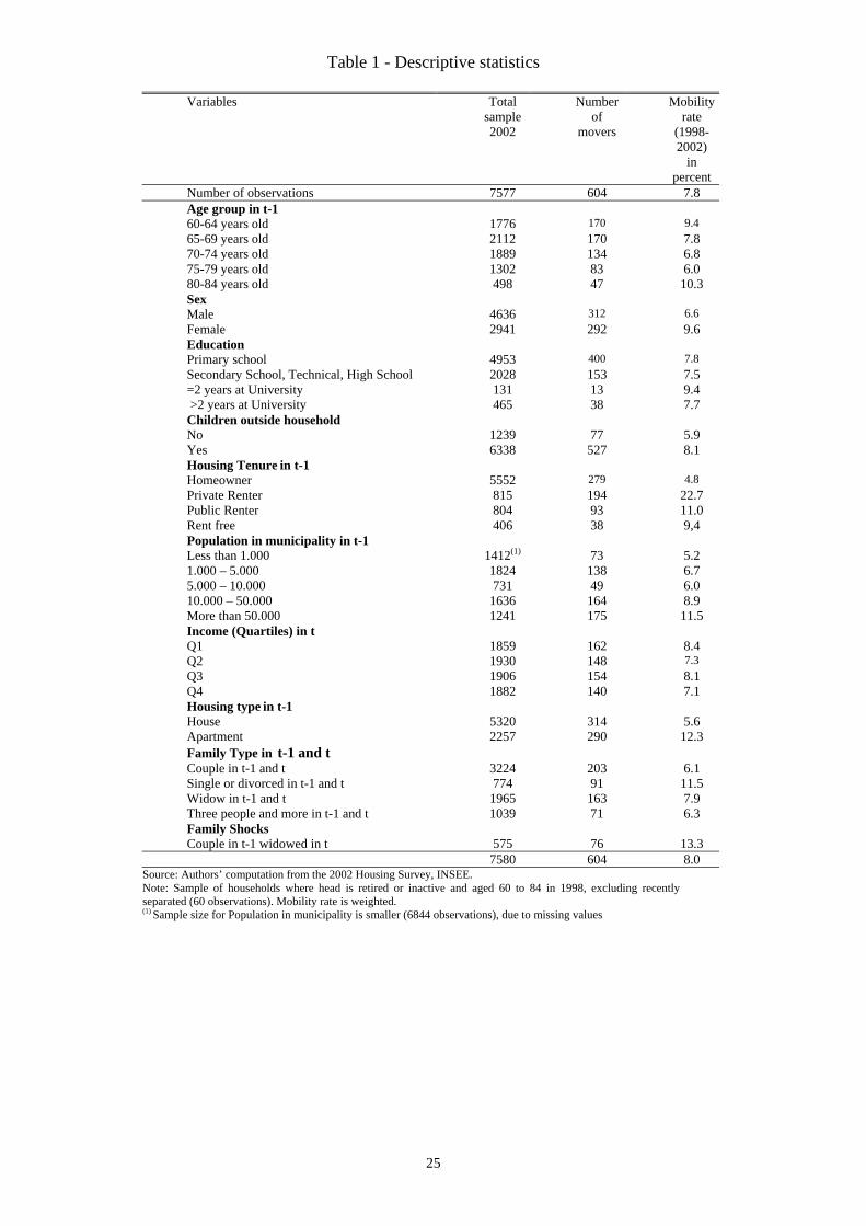
Table 1 - Descriptive statistics

Variables Total sample 2002

Number of

movers

Mobility rate

(1998-2002)

in percent

Number of observations 7577 604 7.8 Age group in t-1 60-64 years old 1776 170 9.4 65-69 years old 2112 170 7.8 70-74 years old 1889 134 6.8 75-79 years old 1302 83 6.0 80-84 years old 498 47 10.3 Sex Male 4636 312 6.6 Female 2941 292 9.6 Education Primary school 4953 400 7.8 Secondary School, Technical, High School 2028 153 7.5 =2 years at University 131 13 9.4 >2 years at University 465 38 7.7 Children outside household No 1239 77 5.9 Yes 6338 527 8.1 Housing Tenure in t-1 Homeowner 5552 279 4.8 Private Renter 815 194 22.7 Public Renter 804 93 11.0 Rent free 406 38 9,4 Population in municipality in t-1 Less than 1.000 1412(1) 73 5.2 1.000 – 5.000 1824 138 6.7 5.000 – 10.000 731 49 6.0 10.000 – 50.000 1636 164 8.9 More than 50.000 1241 175 11.5 Income (Quartiles) in t Q1 1859 162 8.4 Q2 1930 148 7.3 Q3 1906 154 8.1 Q4 1882 140 7.1 Housing type in t-1 House 5320 314 5.6 Apartment 2257 290 12.3 Family Type in t-1 and t Couple in t-1 and t 3224 203 6.1 Single or divorced in t-1 and t 774 91 11.5 Widow in t-1 and t 1965 163 7.9 Three people and more in t-1 and t 1039 71 6.3 Family Shocks Couple in t-1 widowed in t 575 76 13.3 7580 604 8.0

Source: Authors’ computation from the 2002 Housing Survey, INSEE. Note: Sample of households where head is retired or inactive and aged 60 to 84 in 1998, excluding recently separated (60 observations). Mobility rate is weighted. (1) Sample size for Population in municipality is smaller (6844 observations), due to missing values

25

Table 2: Transitions to widowhood by age group

1992-1996 1998-2002

Age group Rate Number of observations

Rate Number of observations

60 – 64 11.5% 98 8.3% 81 65 – 69 11.7% 115 14.2% 157 70 – 74 15.0% 112 17.4% 164 75 – 79 18.4% 63 20.6% 123 80 – 84 23.3% 53 29.8% 50 All 14.4 % 441 15.6 % 575 Source: Authors’ computation from the 1996 and 2002 Housing Surveys, INSEE. Note: The rate of transitions to widowhood is defined for the sample of couples (with head aged 60 to 84 and retired or inactive four years before the survey date), as the ratio between the number of couples experiencing a transition to widowhood to the total number of couples. This rate is weighted.

Table 3: Residential mobility rate by previous family types and family shocks 1996 2002 Family Type in t-1 and t Mobility Rate Number of

observations Mobility Rate Number of

observations Couple in t-1 and t 5.5% 2666 6.2% 3224 Single or divorced in t-1 and t 8.1% 634 11.6% 774 Widow in t-1 and t 6.3% 1754 7.9% 1965 Three people and more in t-1 and t 6.8% 1050 6.4% 1039 Couple in t-1 widowed in t 15.7% 441 13.3% 575 Couple in t-1 Separated in t 28.3% 65 28.2% 60 All 7,1 % 6608 8,0% 7640 Source: Authors’ computation from the 1996 and 2002 Housing Surveys, INSEE. Note: Sample of households where head is retired or inactive and aged 60 to 84 four years before the survey. See the end of section 4 for the definition of family types and transitions.

26

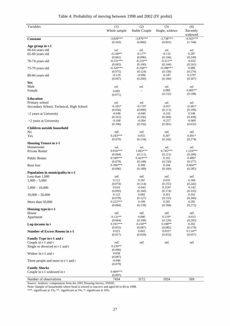
Table 4: Probability of moving between 1998 and 2002 (IV probit)

Variables (1) Whole sample

(2) Stable Couple

(3) Single, widows

(4) Recently widowed

Constant -3.828*** (0.543)

-3.876*** (0.866)

-3.738*** (0.841)

-4.563*** (1.744)

Age group in t-1 60-64 years old ref. ref. ref. ref. 65-69 years old -0.140**

(0.061) -0.177* (0.096)

-0.132 (0.144)

0.287 (0.249)

70-74 years old -0.231*** (0.065)

-0.210** (0.100)

-0.311** (0.144)

-0.032 (0.261)

75-79 years old -0.320*** (0.075)

-0.258** (0.124)

-0.398*** (0.150)

0.088 (0.270)

80-84 years old -0.119 (0.097)

-0.096 (0.200)

-0.187 (0.166)

0.579* (0.307)

Sex Male ref. ref. ref. ref. Female 0.095

(0.071) -

0.089 (0.132)

0.405** (0.198)

Education Primary school ref. ref. ref. ref. Secondary School, Technical, High School -0.105*

(0.056) -0.170* (0.090)

-0.057 (0.111)

-0.381* (0.199)

=2 years at University -0.048 (0.161)

-0.040 (0.256)

-0.101 (0.369)

0.548 (0.438)

>2 years at University -0.168 (0.106)

-0.204 (0.156)

-0.257 (0.281)

-0.909 (0.632)

Children outside household No ref. ref. ref. ref. Yes 0.243***

(0.070) 0.055

(0.134) 0.207

(0.142) 0.491* (0.274)

Housing Tenure in t-1 Homeowner ref. ref. ref. ref. Private Renter 0.916***

(0.064) 1.063*** (0.111)

0.745*** (0.121)

1.124*** (0.206)

Public Renter 0.349*** (0.079)

0.423*** (0.148)

0.102 (0.150)

0.486* (0.277)

Rent free 0.396*** (0.096)

0.309 (0.189)

0.244 (0.160)

0.664** (0.285)

Population in municipality in t-1 Less than 1,000 ref. ref. ref. ref. 1,000 – 5,000 0.112

(0.074) 0.187

(0.114) 0.035

(0.155) 0.168

(0.242) 5,000 – 10,000 0.010

(0.095) -0.043 (0.160)

0.319* (0.174)

-0.142 (0.333)

10,000 – 50,000 0.122 (0.078)

0.092 (0.127)

0.201 (0.155)

0.242 (0.266)

More than 50,000 0.222*** (0.084)

0.199 (0.139)

0.205 (0.168)

0.285 (0.272)

Housing type in t-1 House ref. ref. ref. ref. Apartment 0.131**

(0.064) 0.090

(0.109) 0.219* (0.120)

-0.015 (0.205)

Log-income in t 0.191*** (0.055)

0.218** (0.087)

0.188** (0.085)

0.202 (0.179)

Number of Excess Rooms in t-1 0.023 (0.017)

0.003 (0.029)

0.055* (0.033)

0.114** (0.057)

Family Type in t-1 and t Couple in t-1 and t ref. ref. ref. ref. Single or divorced in t-1 and t 0.239**

(0.096)

Widow in t-1 and t 0.058 (0.087)

Three people and more in t-1 and t -0.046 (0.079)

Family Shocks Couple in t-1 widowed in t 0.404***

(0.097)

Number of observations 7434 3172 1924 569 Source: Authors’ computation from the 2002 Housing Survey, INSEE. Note: Sample of households where head is retired or inactive and aged 60 to 84 in 1998. ***: significant at 1%; **: significant at 5%; *: significant at 10%.

27

Table 5: Variation in the number of rooms when moving, multinomial Logit

Variables Downsizing Upsizing

Constant -2.312** (0.997)

-0.793 (1.060)

Age group in t-1 60-64 years old ref. ref. 65-69 years old -0.390*

(0.230) -0.020 (0.226)

70-74 years old 0.053 (0.240)

-0.660** (0.261)

75-79 years old 1.028*** (0.309)

-0.207 (0.338)

80-84 years old 1.105*** (0.364)

-0.093 (0.400)

Sex Male ref. ref. Female 0.013

(0.262) -0.042 (0.279)

Education Primary school ref. ref. Secondary School, Technical, High School -0.064

(0.213) 0.088

(0.219) =2 years at University 0.130

(0.650) -0.006 (0.709)

>2 years at University -0.737* (0.420)

0.492 (0.381)

Housing Tenure in t-1 Homeowner ref. ref. Private or Public Renter 0.355*

(0.199) -0.258 (0.203)

Population in municipality in t-1 Less than 1,000 ref. ref. 1,000 – 5,000 -0.101

(0.330) -0.400 (0.362)

5,000 – 10,000 0.194 (0.402)

-0.477 (0.433)

10,000 – 50,000 0.075 (0.333)

-0.389 (0.361)

More than 50,000 -0.128* (0.347)

-0.537 (0.371)

Housing type in t-1 House ref. ref. Apartment -0.002

(0.225) 0.056

(0.240) Log-income in t -0.008

(0.085) 0.172* (0.091)

Number of Excess Rooms in t-1 1.169*** (0.098)

-0.384*** (0.102)

Family Type in t-1 and t Couple in t-1 and t ref. ref. Single or divorced in t-1 and t 0.035

(0.339) -0.115 (0.325)

Widow in t-1 and t 0.147 (0.325)

0.108 (0.352)

Three people and more in t-1 and t 1.766*** (0.310)

-0.888*** (0.335)

Family Shocks Couple in t-1 widowed in t 1.449***

(0.360) -0.361 (0.414)

Number of observations 1099 Source: Authors’ computations from the 1996 and 2002 Housing Survey, INSEE. Note: Sample of households which head is retired or inactive and aged 60 to 84 in (t-1). ***: significant at 1%; **: significant at 5%; *: significant at 10%.

28

Table 6: Choosing an apartment when moving, by previous housing type

Variables Apartment in t-

1 House in t-1

Constant -0.371 (1.451)

-1.144 (1.027)

Age group in t-1 60-64 years old ref. ref. 65-69 years old 0.131

(0.289) -0.032 (0.246)

70-74 years old 0.082 (0.323)

0.641** (0.257)

75-79 years old 0.469 (0.426)

0.963*** (0.340)

80-84 years old 0.750 (0.553)

0.516 (0.378)

Sex Male ref. ref. Female 1.079***

(0.352) 0.017

(0.283) Education Primary school ref. ref. Secondary School, Technical, High School -0.100

(0.263) 0.077

(0.236) =2 years at University 0.132

(0.709) 0.372

(0.758) >2 years at University 1.140**

(0.558) 0.497

(0.444) Housing Tenure in t-1 Homeowner ref. ref. Private or Public Renter 0.523**

(0.254) 0.138

(0.216) Population in municipality in t-1 Less than 1,000 ref. ref. 1,000 – 5,000 0.354

(0.727) 0.014

(0.264) 5,000 – 10,000 1.596**

(0.803) 0.806** (0.351)

10,000 – 50,000 1.516** (0.676)

0.723** (0.286)

More than 50,000 1.620** (0.671)

0.817** (0.332)

Housing type in t-1 -0.048 (0.114)

-0.029 (0.092)

House -0.337* (0.104)

0.014 (0.062)

Apartment Log-income in t ref. ref. Number of Excess Rooms in t-1 0.173

(0.402) 1.146*** (0.414)

Widow in t-1 and t 0.415 (0.438)

1.029*** (0.345)

Three people and more in t-1 and t -0.003 (0.374)

0.331 (0.300)

Family Shocks Couple in t-1 widowed in t 0.575

(0.559) 1.189*** (0.349)

Number of observations 536 563 Source: Authors’ computation from the pooled 1996 and 2002 Housing Surveys, INSEE. Note: Sample of households where head is retired or inactive and aged 60 to 84 four years before the survey date. ***: significant at 1%; **: significant at 5%; *: significant at 10%.

29

Table 7: Choosing to be a tenant when moving, by previous housing tenure

Variables Tenant in t-1 Owner in t-1 Constant 3.811***

(1.397) -1.809 (1.131)

Age group in t-1 60-64 years old ref. ref. 65-69 years old 0.816***

(0.320) 0.585** (0.282)

70-74 years old 0.468 (0.341)

1.140*** (0.291)

75-79 years old 0.833* (0.445)

1.208*** (0.353)

80-84 years old 0.268 (0.530)

1.111*** (0.370)

Sex Male ref. ref. Female 0.677**

(0.355) 0.268

(0.300) Education Primary school ref. ref. Secondary School, Technical, High School -0.752***

(0.282) -0.481** (0.240)

=2 years at University -1.540** (0.760)

-0.687 (0.817)

>2 years at University 0.045 (0.571)

-1.042** (0.500)

Housing Tenure in t-1 Homeowner ref. ref. Private or Public Renter -0.208

(0.343) -0.383 (0.271)

Population in municipality in t-1 Less than 1,000 ref. ref. 1,000 – 5,000 0.056

(0.555) 0.476

(0.321) 5,000 – 10,000 1.517*

(0.885) 0.331

(0.403) 10,000 – 50,000 0.385

(0.563) 0.050

(0.335) More than 50,000 -0.267

(0.568) 0.208

(0.355) Housing type in t-1 -0.243**

(0.122) 0.007

(0.099) House -0.277**

(0.111) -0.121* (0.068)

Apartment Log-income in t ref. ref. Number of Excess Rooms in t-1 0.533

(0.431) 1.354*** (0.429)

Widow in t-1 and t 0.181 (0.445)

1.360*** (0.367)

Three people and more in t-1 and t 0.320 (0.403)

0.589* (0.343)

Family Shocks Couple in t-1 and widowed in t 0.278

(0.500) 0.975*** (0.381)

Number of observations 528 571 Source: authors’ computation from the pooled 1996 and 2002 Housing Surveys, INSEE. Note: sample of mobile households with a head aged 60 to 84 and retired or inactive four years before the survey date.

30

Table 8: Variation in the municipality size when moving, multinomial Logit

Variables Smaller size Bigger size Constant -3.871***

(1.076) 0.074

(0.980) Age group in t-1 60-64 years old ref. ref. 65-69 years old -0.098

(0.214) -0.418* (0.232)

70-74 years old -0.128 (0.233)

0.135 (0.241)

75-79 years old 0.363 (0.278)

0.410 (0.300)

80-84 years old -0.108 (0.328)

-0.532 (0.353)

Sex Male ref. ref. Female -0.022

(0.254) -0.396 (0.263)

Education Primary school ref. ref. Secondary School, Technical, High School 0.453**

(0.188) 0.677*** (0.218)

=2 years at University -0.159 (0.638)

0.739 (0.609)

>2 years at University 0.216 (0.344)

1.231*** (0.416)

Housing Tenure in t-1 Homeowner ref. ref. Private or Public Renter 0.488**

(0.214) 0.394* (0.233)

Population in municipality in t-1 Less than 1,000 ref. ref. 1,000 – 5,000 -0.795***

(0.185) -0.990***

(0.200) 5,000 – 10,000 10,000 – 50,000 ref. ref. More than 50,000 1.204*

(0.644) -0.871***

(0.267) Housing type in t-1 1.462**

(0.671) -1.513***

(0.337) House 1.435**

(0.630) -2.463***

(0.300) Apartment 1.571**

(0.634) -4.234***

(0.422) Log-income in t 0.172**

(0.080) 0.114

(0.087) Number of Excess Rooms in t-1 0.081

(0.063) -0.014 (0.063)

Family Type in t-1 and t Couple in t-1 and t ref. ref. Single or divorced in t-1 and t -0.534

(0.317) 0.182

(0.350) Widow in t-1 and t -0.396

(0.313) 0.354

(0.325) Three people and more in t-1 and t -0.468*

(0.276) -0.110 (0.289)

Family Shocks Couple in t-1 widowed in t -0.323

(0.345) 0.944*** (0.339)

Number of observations 1099 Source: authors’ computation from the 1996 and 2002 Housing Survey, INSEE. Note: sample of households which head is retired or inactive and aged 60 to 84 in (t-1). ***: significant at 1%; **: significant at 5%; *: significant at 10%.

31

Table 9: Reasons for moving, by family type or transition

Transition to widowhood

Couple Single, widow

Type of reason Retirement - 3.9 0.6 Personal or family reasons1

Among them: get closer to family or friends, went back to birthplace

27.225.9

13.112.1

16.5 15.3

Environment or location2 12.8 20.6 16.0 Dwelling size or comfort3

Among them; the dwelling quality was too bad wanted a smaller dwelling

18.90.9

17.5

19.97.94.9

27.2 11.112.1

Type of dwelling4 7.1 6.7 4.7 Housing tenure5 6.9 6.8 7.4 Income constraint6 1.0 1.2 1.8 Obligation to move7 3.5 7.0 6.4 Other reason 23.6 20.8 20.4 Number of observations 78 168 117

Source: Authors’ computation from the 1996 Housing Survey, INSEE. Note: Sample of mobile households where head is retired or inactive and aged 60 to 84 in 1992.

1 Separated from partner, got closer to family or friends, went back to birthplace, looked for a better climate (this item cannot be separated from the preceding reason). 2 Unattractive or insecure neighbourhood, neighbours were unsuitable (too noisy, behavioural problems), too far from town centre and community facilities, wanted to get closer to town centre, wanted to live in a less urbanized place. 3 Wanted a larger/smaller dwelling, the dwelling quality was too bad 4 Wanted to live in a house/in an apartment. 5 Wanted to become owner/tenant, found accommodation that could be used for free 6 Wanted to reduce housing expenses (rent, utilities, maintenance cost) 7 Lived temporarily in the dwelling, was expelled by the owner

32

Table 10: Living less than 25 kilometres from closest independent child,

by family type, for mobile and non mobile households

Family Type in t-1 and t estimated parameter

Mobile ref.

Couple in t-1 and t

Non mobile 0.476*** (0.163)

Mobile -0.160 (0.336)

Widow in t-1 and t

Non mobile -0.278 (0.214)

Mobile 0.334 (0.270)

Single or divorced in t-1 and t

Non mobile 0.205 (0.189)

Mobile 0.706* (0.365)

3 people or more in t-1 and t

Non mobile 0.649*** (0.180)

Mobile 0.827** (0.377)

Couple in t-1 widowed in t

Non mobile 0.166 (0.206)

Source: Authors’ computation from the 2002 Housing Survey, INSEE. Note: Sample of households where head is retired or inactive and aged 60 to 84 in 1997 with at least one child who lives independently, and no child at home. We estimate a logit model of having a child living less than 25 kilometres from the household. Other controls are age groups in t-1, sex, education level, housing type and tenure in t-1, population in municipality in t-1 and log income in t.

33

Figure 1 – Percentage of widows (W) and widowers (M) by age for five birth cohorts

Figure 2 – Average household income by age and birth cohort

Note: income i rt

0%

10%

20%

30%

40%

50%

60%

70%

80%

90%

60 61 62 63 64 65 66 67 68 69 70 71 72 73 74 75 76 77 78 79 80 81 82 83 84 85 86 87 88 89 90

1900 W 1920 W 1930 W1940 W 1910 W 1900 M1910 M 1920 M 1930 M1940 M

Source: French register of civil status (Etat Civil).

5

10

15

20

25

30

60 64 68 72 76 80 84 88Age

1940 1932 19241916 1908 19001892

Source: Laferrère (2005), computation from the 1973, 1978, 1984, 1988, 1992, 1996 and 2002 Housing Surveys, INSEE.

s expressed in thousands of 2001 euros. Cohorts are four-year cohorts. For instance, the 1940 cohoincludes all the households born during the 1937-1940 period.

34

Figure 3 – Living arrangements of widows by age, in 1999

0%

10%

20%

30%

40%

50%

60%

70%

80%

90%

60 - 64 65 - 69 70 - 74 75 - 79 80 - 84 85 - 89 90 - 94 95 - 99 100 andoverAge

Institution AloneWith a partner and/or childrenWith Others

Source: constructed from the 1999 French Census. Note: the sample excludes widowers. “With others” describes households with at least two members, other than a child or a partner.

35

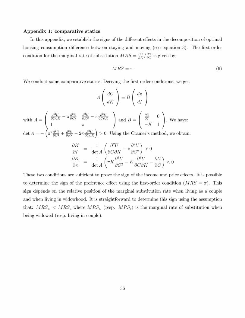
Appendix 1: comparative statics

In this appendix, we establish the signs of the di¤erent e¤ects in the decomposition of optimal

housing consumption di¤erence between staying and moving (see equation 3). The �rst-order

condition for the marginal rate of substitution MRS = @U@K=@U@Cis given by:

MRS = � (6)

We conduct some comparative statics. Deriving the �rst order conditions, we get:

A

0@ dC

dK

1A = B

0@ d�

dI

1A

with A =

0@ @2U@C@K

� � @2U@C2

@2U@K2 � � @2U

@C@K

1 �

1A and B =

0@ @U@C

0

�K 1

1A. We have:detA = �

��2 @

2U@C2

+ @2U@K2 � 2� @2U

@C@K

�> 0. Using the Cramer�s method, we obtain:

@K

@I=

1

detA

�@2U

@C@K� �@

2U

@C2

�> 0

@K

@�=

1

detA

��K

@2U

@C2�K @2U

@C@K� @U@C

�< 0

These two conditions are su¢ cient to prove the sign of the income and price e¤ects. It is possible

to determine the sign of the preference e¤ect using the �rst-order condition (MRS = �). This

sign depends on the relative position of the marginal substitution rate when living as a couple

and when living in widowhood. It is straightforward to determine this sign using the assumption

that: MRSw < MRSc where MRSw (resp. MRSc) is the marginal rate of substitution when

being widowed (resp. living in couple).

36

Appendix 2: Widows do not move to live with their children

We want to appraise whether moves of recent widows to co-reside with a child are frequent.

Indeed, these moves are ignored in our study but living with kinship could be a way to adjust

one�s housing consumption (Börsch-Supan, 1990). We identify a household possibly containing a

widow that moved to her children�s place using three criteria. First, the household must include a

60� 84 year-old widow that is not the reference person. Second, the household size must increaseby one in the four-year period before the survey date. Third, this increase should not be due

to obvious demographic reasons that are not related to the arrival of a widow like a birth or

household formation.

In fact, 258 households include a widow who is between 60 and 84 years old in the 2002 Housing

Survey (�rst criterion). Among them, only 13 percent experience a one-person increase in the size

of the household (second criterion). Finally, among the remaining households, only 41 percent

may have experienced the arrival of a widow (third criterion). Overall, there are only 14 house-

holds meeting the three criteria. This is very few considering that not all may have experienced

widowhood recently. In conclusion, only very few widows move to their children�s places after

their spouse�s death and use kinship to adjust their housing consumption.

37

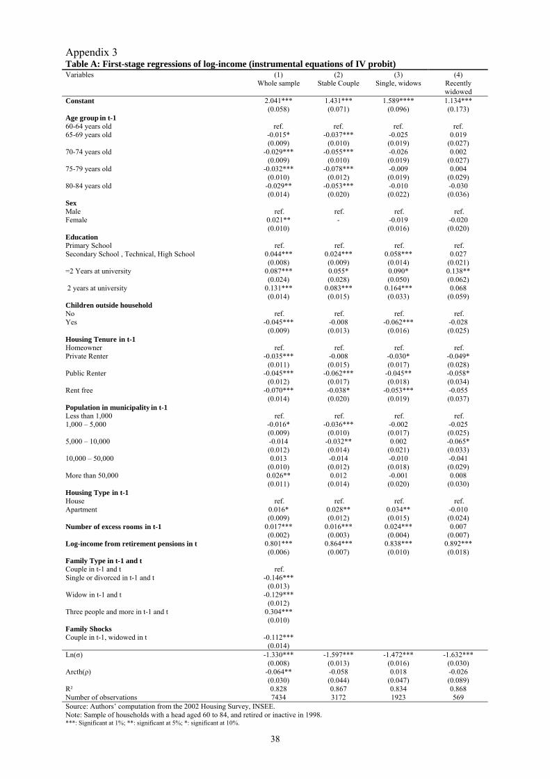
Appendix 3 Table A: First-stage regressions of log-income (instrumental equations of IV probit) Variables (1)

Whole sample (2)

Stable Couple (3)

Single, widows (4)

Recently widowed

Constant 2.041*** (0.058)

1.431*** (0.071)

1.589**** (0.096)

1.134*** (0.173)

Age group in t-1 60-64 years old ref. ref. ref. ref. 65-69 years old -0.015*

(0.009) -0.037***

(0.010) -0.025 (0.019)

0.019 (0.027)

70-74 years old -0.029*** (0.009)

-0.055*** (0.010)

-0.026 (0.019)

0.002 (0.027)

75-79 years old -0.032*** (0.010)

-0.078*** (0.012)

-0.009 (0.019)

0.004 (0.029)

80-84 years old -0.029** (0.014)

-0.053*** (0.020)

-0.010 (0.022)

-0.030 (0.036)

Sex Male ref. ref. ref. ref. Female 0.021**

(0.010) -

-0.019 (0.016)

-0.020 (0.020)

Education Primary School ref. ref. ref. ref. Secondary School , Technical, High School 0.044***

(0.008) 0.024*** (0.009)

0.058*** (0.014)

0.027 (0.021)

=2 Years at university 0.087*** (0.024)

0.055* (0.028)

0.090* (0.050)

0.138** (0.062)

2 years at university 0.131*** (0.014)

0.083*** (0.015)

0.164*** (0.033)

0.068 (0.059)

Children outside household No ref. ref. ref. ref. Yes -0.045***

(0.009) -0.008 (0.013)

-0.062*** (0.016)

-0.028 (0.025)

Housing Tenure in t-1 Homeowner ref. ref. ref. ref. Private Renter -0.035***

(0.011) -0.008 (0.015)

-0.030* (0.017)

-0.049* (0.028)

Public Renter -0.045*** (0.012)

-0.062*** (0.017)

-0.045** (0.018)

-0.058* (0.034)

Rent free -0.070*** (0.014)

-0.038* (0.020)

-0.053*** (0.019)

-0.055 (0.037)

Population in municipality in t-1 Less than 1,000 ref. ref. ref. ref. 1,000 – 5,000 -0.016*

(0.009) -0.036***

(0.010) -0.002 (0.017)

-0.025 (0.025)

5,000 – 10,000 -0.014 (0.012)

-0.032** (0.014)

0.002 (0.021)

-0.065* (0.033)

10,000 – 50,000 0.013 (0.010)

-0.014 (0.012)

-0.010 (0.018)

-0.041 (0.029)

More than 50,000 0.026** (0.011)

0.012 (0.014)

-0.001 (0.020)

0.008 (0.030)

Housing Type in t-1 House ref. ref. ref. ref. Apartment 0.016*

(0.009) 0.028** (0.012)

0.034** (0.015)

-0.010 (0.024)

Number of excess rooms in t-1 0.017*** (0.002)

0.016*** (0.003)

0.024*** (0.004)

0.007 (0.007)

Log-income from retirement pensions in t 0.801*** (0.006)

0.864*** (0.007)

0.838*** (0.010)

0.892*** (0.018)

Family Type in t-1 and t Couple in t-1 and t ref. Single or divorced in t-1 and t -0.146***

(0.013)

Widow in t-1 and t -0.129*** (0.012)

Three people and more in t-1 and t 0.304*** (0.010)

Family Shocks Couple in t-1, widowed in t -0.112***

(0.014) Ln(σ) -1.330***

(0.008) -1.597***

(0.013) -1.472***

(0.016) -1.632***

(0.030) Arcth(ρ) -0.064**

(0.030) -0.058 (0.044)

0.018 (0.047)

-0.026 (0.089)

R² 0.828 0.867 0.834 0.868 Number of observations 7434 3172 1923 569 Source: Authors’ computation from the 2002 Housing Survey, INSEE. Note: Sample of households with a head aged 60 to 84, and retired or inactive in 1998. ***: Significant at 1%; **: significant at 5%; *: significant at 10%.

38

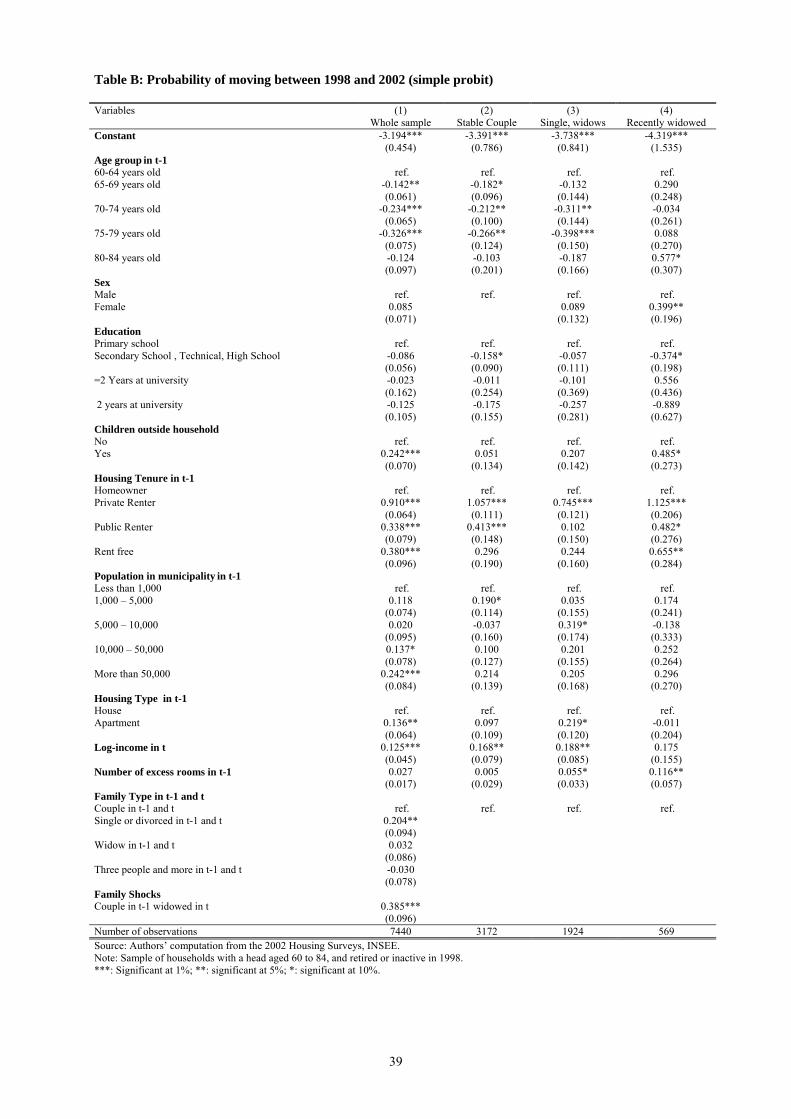
Table B: Probability of moving between 1998 and 2002 (simple probit) Variables (1)

Whole sample (2)

Stable Couple (3)

Single, widows (4)

Recently widowed Constant -3.194***

(0.454) -3.391***

(0.786) -3.738***

(0.841) -4.319***

(1.535) Age group in t-1 60-64 years old ref. ref. ref. ref. 65-69 years old -0.142**

(0.061) -0.182* (0.096)

-0.132 (0.144)

0.290 (0.248)

70-74 years old -0.234*** (0.065)

-0.212** (0.100)

-0.311** (0.144)

-0.034 (0.261)

75-79 years old -0.326*** (0.075)

-0.266** (0.124)

-0.398*** (0.150)

0.088 (0.270)

80-84 years old -0.124 (0.097)

-0.103 (0.201)

-0.187 (0.166)

0.577* (0.307)

Sex Male ref. ref. ref. ref. Female 0.085

(0.071) 0.089

(0.132) 0.399** (0.196)

Education Primary school ref. ref. ref. ref. Secondary School , Technical, High School -0.086

(0.056) -0.158* (0.090)

-0.057 (0.111)

-0.374* (0.198)

=2 Years at university -0.023 (0.162)

-0.011 (0.254)

-0.101 (0.369)

0.556 (0.436)

2 years at university -0.125 (0.105)

-0.175 (0.155)

-0.257 (0.281)

-0.889 (0.627)

Children outside household No ref. ref. ref. ref. Yes 0.242***

(0.070) 0.051

(0.134) 0.207

(0.142) 0.485* (0.273)

Housing Tenure in t-1 Homeowner ref. ref. ref. ref. Private Renter 0.910***

(0.064) 1.057*** (0.111)

0.745*** (0.121)

1.125*** (0.206)

Public Renter 0.338*** (0.079)

0.413*** (0.148)

0.102 (0.150)

0.482* (0.276)

Rent free 0.380*** (0.096)

0.296 (0.190)

0.244 (0.160)

0.655** (0.284)

Population in municipality in t-1 Less than 1,000 ref. ref. ref. ref. 1,000 – 5,000 0.118

(0.074) 0.190* (0.114)

0.035 (0.155)

0.174 (0.241)

5,000 – 10,000 0.020 (0.095)

-0.037 (0.160)

0.319* (0.174)

-0.138 (0.333)

10,000 – 50,000 0.137* (0.078)

0.100 (0.127)

0.201 (0.155)

0.252 (0.264)

More than 50,000 0.242*** (0.084)

0.214 (0.139)

0.205 (0.168)

0.296 (0.270)

Housing Type in t-1 House ref. ref. ref. ref. Apartment 0.136**

(0.064) 0.097

(0.109) 0.219* (0.120)

-0.011 (0.204)

Log-income in t 0.125*** (0.045)

0.168** (0.079)

0.188** (0.085)

0.175 (0.155)

Number of excess rooms in t-1 0.027 (0.017)

0.005 (0.029)

0.055* (0.033)

0.116** (0.057)

Family Type in t-1 and t Couple in t-1 and t ref. ref. ref. ref. Single or divorced in t-1 and t 0.204**

(0.094)

Widow in t-1 and t 0.032 (0.086)

Three people and more in t-1 and t -0.030 (0.078)

Family Shocks Couple in t-1 widowed in t 0.385***

(0.096)

Number of observations 7440 3172 1924 569 Source: Authors’ computation from the 2002 Housing Surveys, INSEE. Note: Sample of households with a head aged 60 to 84, and retired or inactive in 1998. ***: Significant at 1%; **: significant at 5%; *: significant at 10%.

39