=

= NASA CONTRACTOR NASA

REPORT

...... z

• iCR-1061 i

I-i

i!1

I

N 68-_t fib _5

t (ACCL_ION_ - (THRU)< 23 (£') ¢COD<

(NASA CIt OR TMX OR AD NUMBER) (CATEO'ORY)

AN

C

AND

Part _....... .IJt

Finite

of Char

Chemic:

Prepared

iTEK

Palo Alto,

for

_ NATIONAL

L.Z'I..I. Is, l_..

GPO PRICE $

CFSTI PRICE(S) $

Hard copy (HC)

Microfiche (MF)

ff653 July 65

!!

https://ntrs.nasa.gov/search.jsp?R=19680017220 2018-07-22T13:13:49+00:00Z

_--:: : -- . ....................................................................._...................................................;::::::_3£ _...............: _ ............................................_ __: __ .............

.._ ................................_ _ ....... _ ..........................._ ........_ _

NASA CR- 1061

AN ANALYSIS OF THE COUPLED CHEMICALLY REACTING

BOUNDARY LAYER AND CHARRING ABLATOR

Part II

Finite Difference Solution for the In-Depth Response

of Charring Materials Considering Surface

Chemical and Energy Balances

By Carl B. Moyer and Roald A. Rindal

Distribution of this report is provided in the interest of

information exchange. Responsibility for the contents

resides in the author or organization that prepared it.

Issued by Originator as Aerotherm Report No. 66-7, Part II

Prepared under Contract No. NAS 9-4599 by

ITEK CORPORATION, VIDYA DIVISION

Palo Alto, Calif.

for Manned Spacecraft Center

NATIONAL AERONAUTICS AND SPACE ADMINISTRATION

For sale by the Clearinghouse for Federal S¢ientlfic and Technical Information

Springfield, Virginia 22151 - CFSTI price $3.00

PRECEDING PAGE BLANK NOT FILMED.

ABSTRACT

This report presents an analysis of the in-depth response of materials

exposed to a high temperature environment, and describes a computer program

based upon the analysis.

The differential equations for the in-depth response are formulated

and then cast into a finite difference form implicit in temperature. Three

pyrolyzing constituents are allowed, with an accurate model of observed py-

rolysis kinetics. Heat flow in-depth is one-dimensional, but cross-section

area may vary with depth.

The program for in-depth response computation may be coupled to a variety

of boundary conditions. One of the possible boundary conditions is a com-

plete boundary layer solution described in other reports of this series.

Another version of the program may be coupled to a general film coefficient

model of the boundary layer; this boundary condition is described in some de-

tail in the present report.

The report concludes with sample solutions generated by the computer

program.

iii

r_ a

PRECEDING PAGE BLANK NOT FILMED.

FOREWORD

The present report is one of a series of six reports, published simul-

taneously, which describe analyses and computational procedures for: i) pre-

diction of the in-depth response of charring ablation materials, based on one-

dimensional thermal streamtubes of arbitrary cross-section and considering

general surface chemical and energy balances, and 2) nonsimilar solution of

chemically reacting laminar boundary layers, with an approximate formulation

for unequal diffusion and thermal diffusion coefficients for all species and

with a general approach to the thermochemical solution of mixed equilibrium-

nonequilibrium, homogeneous or heterogeneous systems. Part I serves as a

summary report and describes a procedure for coupling the charring ablator

and boundary layer routines. The charring ablator procedure is described in

Part II, whereas the fluid-mechanical aspects of the boundary layer and the

boundary-layer solution procedure are treated in Part III. The approximations

for multicomponent transport properties and the chemical state models are

described in Parts IV and V, respectively. Finally, in Part VI an analysis

is presented for the in-depth response of charring materials taking into ac-

count char-density buildup near the surface due to coking reactions in depth.

The titles in the series are:

Part I Summary Report: An Analysis of the Coupled Chemically Reacting

Boundary Layer and Charring Ablator, by R. M. Kendall, E. P.

Bartlett, R. A. Rindal, and C. B. Moyer.

Part II Finite Difference Solution for the In-depth Response of Charring

Materials Considering Surface Chemical and Energy Balances, by

C. B. Moyer and R. A. Rindal.

Part III Nonsimilar Solution of the Multicomponent Laminar Boundary Layer

by an Integral Matrix Method, by E. P. Bartlett and R. M. Kendall.

Part IV A Unified Approximation for Mixture Transport Properties for Multi-

component Boundary-Layer Applications, by E. P. Bartlett, R. M.

Kendall, and R. A. Rindal.

Part V A General Approach to the Thermochemical Solution of Mixed Equilib-

rium-Nonequilibrium, Homogeneous or Heterogeneous Systems, by

R. M. Kendall.

Part VI An Approach for Characterizing Charring Ablator Response with In-

depth Coking Reactions, by R. A. Rindal.

This effort was conducted for the Structures and Mechanics Division of

the Manned Spacecraft Center, National Aeronautics and Space Administration

under Contract No. NAS9-4599 to Vidya Division of Itek Corporation with Mr.

Donald M. Curry and Mr. George Strouhal as the NASA Technical Monitors. The

work was initiated by the present authors while at Vidya and was completed

by Aerotherm Corporation under subcontract to Vidya (P.O. 8471 V9002) after

Aerotherm purchased the physical assets of the Vidya Thermodynamics Depart-

ment. Dr. Robert M. Kendall of Aerotherm was the Program Manager and Prin-

cipal Investigator.

rf...=_D[i-_,:j pA,"n ,_, ,,.

TABLE OF CONTENTS

ABSTRACT

FOREWORD

LIST OF FIGURES

LIST OF SYMBOLS

I. GENERAL INTRODUCTION

2.

iii

V

xi

i

PROBLEM DESCRIPTION AND HISTORICAL ORIENTATION i

2.1 General Remarks 1

2.2 Problem Description 2

2.3 Problem History 3

ANALYSIS AND COMPUTATIONAL PROCEDURE FOR CHARRING MATERIAL

RESPONSE 4

3.1 Problem Formulation 4

3.1.i Introduction 4

3.1.2 Basic Differential Equations 4

3.1.3 Boundary Conditions 6

3.2 Finite Difference Development 7

3.2.1 Introduction 7

3.2.2 Differencing Philosophy 8

3.2.3 Transformation of Differential Equations 9

3.2.3.1 General Remarks 9

3.2.3.2 Geometrical Considerations i0

3.2.3.3 Conservation of Mass in Moving Coordinate System i0

3.2.4 Difference Forms 18

3.2.4.1 Mass Equation 18

3.2.4.1.1 Nodes other than the first or last 18

3.2.4.1.2 The surface node 22

3.2.4.1.3 The last ablating node 22

3.2.4.2 Energy Equation 23

3.2.4.2.1 Nodes other than the first or last 23

3.2.4.2.2 The surface node 25

3.2.4.2.3 The last ablating node 27

3.2.4.2.4 Back-up nodes 28

3.2.4.2.5 Last node 28

3.3 Solution Structure Preparatory to Coupling to the Surface

Boundary Condition 28

3.3.1 Tri-diagonal Formulation of the Finite Difference

Energy Relations 28

3.3.2 Solution of Mass Relations and Evaluation of Tri-diagonal

Matrix Elements 29

3.

vii

TABLE OF CONTENTS (Continued)

4o

3o

3.4

3

3

3

3

3.5

3.6

SOME

4.1

4.2

4.3

4.4

4.5

4.6

4.7

4.8

4.9

4.10

4.11

4.12

3.3 Reduction of Tri-diagonal Matrix to Surface EnergyRelation

Coupling In-Depth Response to Surface Energy Balance

.4.1 General Form of Energy Relation

.4.2 Tabular Formulation of Surface Quantities

.4.3 Solution Procedure for the Surface Energy Balance

.4.4 Completing the In-depth Solution

Solution Without Energy Balance

Solution with Radiation Input Only and No Recession

NOTES ON PROPERTY VALUES

Introduction

Densities

Kinetic Data

Specific Heats

Heat of Formation

Heat of Pyrolysis

Pyrolysis Gas Enthalpy

Thermal Conductivity

Surface Emissivity

Heat of Ablation, Heat of Combustion

Surface Species

Conclusion

3O

3O

3O

31

32

33

34

35

35

35

35

36

36

36

37

38

39

39

39

5. NOTES ON FILM COEFFICIENT MODEL OF THE BOUNDARY LAYER WITH

HEAT TRANSFER, MASS TRANSFER, AND CHEMICAL REACTION 40

5.1 Introduction 40

5.2 General Position, Importance, and History of Film Coefficient

Models Applied to Mass Transfer with Chemical Reactions 40

5.2.1 General Remarks 40

5.2.2 History of Film Coefficient Model for C M / C H 42

5.2.3 History of Extension to Unequal Mass Diffusion

Coefficients 43

5.3 Discussion of Film Coefficient Expressions 43

5.3.1 Mass Transfer 43

5.3.2 Energy Equations 44

5.4 Use of Film Coefficient Equations to Calculate Surface

Energy Balance 48

5.4.1 Basic Aspects 48

5.4.2 Input and Correction of Heat Transfer Coefficient 49

5.5 Conclusions 50

6. PRESSURE DROP 50

6.1 Pressure Drop Correlation Equation 50

viii

TABLEOFCONTENTS(Concluded)

6.2 Finite Difference Formulation

7. SOMEOPERATIONALDETAILSOFTHEAEROTHERMCHARRINGMATERIALABLATIONPROGRAM,VERSION27.1 Introcution7.2 ProgramDescription

7.2.1 GeneralRemarks7.2.2 ProgramObjectives7.2.3 ProgramCapabilities7.2.4 Solution Procedure7.2.5 Output Information7.2.6 Operational Details

7.2.6.1 Storage Requirements7.2.6.2 RunningTime

7.3 SampleProblemSolutions7.3.1 SomeTypical Problems7.3.2 Additional Examples

8. SUMMARYANDCONCLUSION8.1 General Remarks

8.2 Experience with the In-depth Solution Routine (CMA)

8.3 Conclusion

REFERENCES

FIGURES

APPENDIX A - Equations for Coefficients A n , B n, C n, and D n

in In-Depth Energy Equation Array-

APPENDIX B - Conduction Solution Check-Out of the Charring

Material Ablation Program

SUB-APPENDIX B-I - Error Analysis of Steady State Solution for a

Constant Properties Semi-lnfinite Receding Solid

with Constant Surface Temperature and Constant

Surface Recession Rate

APPENDIX C - Study of Alternative Treatments of the Decomposition

Kinetics Equation in the Charring Material Ablation

Program

SUB-APPENDIX C-I - Notes on Problem Specification

SUB-APPENDIX C-2 - Estimation of Execution Time

APPEXDIX D - Transformation of the In-Depth Energy Equation

52

53

53

53

53

54

54

55

55

56

56

56

56

56

56

57

58

58

59

63

ix

4

LIST OF FIGURES

i. Geometrical Configuration and Coordinate System Illustration

2. Finite Difference Representation

3. Experimentally Determined Coefficients for Flow Through

Porous Media

4. Typical Output Page

5. Predicted Degradation Depth Histories, Nylon Phenol_c Reentry

Problem

6. Predicted Temperature Histories at Surface and Selected

Thermocouple Locations, Nylon Phenolic Reentry Problem

7. Typical Machine Plotted Isotherm Depths

63

64

65

66

67

68

69

LISTOFSYMBOLS

A

ABW

An

A*n

B

Bn

B*n

B'

B'C

B'g

C H

CH 0

C M

C n

Cp

D n

D*n

D

_ij

E/R,Ei/R

F

Pi,Pj

F3,F4,F 5

cross section area for a node

area of back wall of last node

coefficient in Eq. (58). See also Appendix A.

value of A after first pass of Gauss

reduction, _ee Eq. (62)

pre-exponential factor,Eq. (3)

coefficient in Eq. (58). See also Appendix A

value of B after first pass of Gauss

reduction, _ee Eq. (62)

defined as B' + B'c g

defined as mc/PeUeCM

defined as m/PeUeC M

Stanton number for heat transfer (corrected

for "blowing", if necessary)

Stanton number for heat transfer not

corrected for blowing

Stanton number for mass transfer

coefficient in Eq. (58). See also Appendix A

specific heat

coefficient in Eq. (58). See also Appendix A

value of D after first pass of Gauss

reduction, _ee Eq. (62)

constant defined by Eq. (69)

binary diffusion coefficient

activation energy for decomposition

radiation view factor

empirical factors appearing in Eq. (69)

general denotations for functional relation-

ship, Eqs. (58), (59)

(ft _ )

(ft _ )

(Btu/ft a OF)

(Btu/ft _ °F)

(see-I)

(Btu/ft 3 OF)

(Btu/ft 3 OF)

(---_

(---)

(---)

(---)

(---)

(---)

(Btu/ft _ sec)

(Btu/Ib OF)

(Btu/ft _ )

(Btu/ft 3 )

(ft _/s ec)

(ft _/see)

(°R)

(---)

(---)

(---)

xi

f

H

h

T b

h s

h%1

hW

S

I

J

J

,y

3kW

K

K i

KN

k

k i

L

Le

%

m.1

LIST OF SYMBOLS (Continued)

general denotation for functional relationship

recovery enthalpy

enthalpy

sensible enthalpy measured above tempera-

ture T b

enthalpy of species i a__t temperature T b

enthalpy of gases adjacent to the wall

enthalpy term defined at Eq. (38)

total number of identifiable species

number of nodelets per node

nodelet index

diffusion flux of element k away from wall

total number of elements in system

mass fraction of species i

mass fraction of element k (regardless of

molecular configuration

kinetic energy contribution to recovery

enthalpy

thermal conductivity, also element index

pre-exponential factor for constituent i,

analogous to B

total number of nodes

Lewis number P_ijCp/k

system molecular weight Ixi_i

system molecular weight, pyrolysis gas

molecular weight of species i

reaction order for constituent i, see Eq. (i0)

mass flow rate per unit area from the

surface

xii

------)

(Btu/ib)

(Btu/lb)

(Btu/ib)

(Btu/ib)

(Btu/ib)

(---)

(---)

(---)

(---)

(ib/ft 2 sec)

(---)

(---)

(---)

(Btu/ib)

(Btu/ft sec° F)

or (---)

(see-_)

(---)

(---)

(ib/ib mole)

( ib/ib mole)

( ib/Ib mole)

(---)

( ib/ft _ see)

I,ISTOFSYMBOLS(Continued)

C

g

gs"

N

NBM

NL

q

qcond

qdiff

qrad in

qrad out

q*

r°f°

R

T,t

Tw, T 1

T

Ue

V

X.l

mass flow rate of char per unit surface area

mass flow rate of pyrolysis gas through a

node

mass flow rate of gas out a unit area of

surface

total number of nodes

denotes first node of back-up material

denotes last node of ablation material

heat absorption term for decomposition

rate of energy conduction into solid

material at surface

rate of energy input to solid surface by

diffusional processes in the boundary layer

rate of energy input to the surface by

radiation from the boundary layer or from

outside the boundary layer

rate of energy radiated away from surface

rate of energy removal from surface with

condensed phases

boundary layer recovery factor

universal gas constant

distance from original location of receding

surface to current surface location

rate of change of S (surface recession

rate)

temperature

wall (surface) temperature

reference temperature for viscosity Eq. (82)

velocity of gases at edge of boundary layer

gas velocity (see pv)

coordinate normal to ablating surface,

fixed to receding surface

PP { 0c )----- 1 --

virgin mass fraction, x 0p- Pc -_

mole fraction of species i

coordinate normal to ablating surface,

origin fixed in space relative to back wall

(ib/ft _ sec)

(ib/sec)

(Ib/ft 2 sec)

(---)

(---)

(---)

(Btu/ib)

(Btu/ft _ sec)

(Btu/ft 2 see)

(Btu/ft _ sec)

(Btu/ft _ sec)

(Btu/ft = sec)

(---)

ft# 1

ib-mole ° R I

(ft)

(ft/sec)

(°R)

(OR)

(°R)

(ft/sec)

(ft/sec)

xiii

LIST OF SYMBOLS (Continued)

Z.l

Z_1

diffusion driving force =K i

see

Eq. (67)

modified Z i defined by Eq. (66)

Z* for elements k independent of molecular

configuration, defined by Eq. (65)

Greek

Ski

W

Y

F

A

Ae

6

C

P

e w

e

u 2

p

pCp

(_v)W

coefficient in Eq. (81)

mass fraction of element k in species i

absorptivity of the wall

coefficient in Eq. (817

constant equal to 2/3 on empirical basis

volume fraction of resin in plastic, see

Eq. (4)

denotes change

time step in finite difference solution

nodal thickness

error in an equation supposed to equal

zero, departure from zero

volume fraction of imagined undecomposed

material in a sample of partially degraded

material

emissivity of the wall

time

viscosity of pyrolysis gas

dimensionless factor defined by Eq. (68)

density

mean volume capacity defined by Eq. (28)

c %

(ft -2 )

(---5

(---)

(ft-15

(---5

ftaresin

ft a material

(---5

(---7

(ft5

(various 5

ftavirqin

ft3material

(---5

(ib/ft-sec)

(---)

(ib/ft35

(Btu/ft 3 °R 5

(Ib/ft 2 sec)

xiv

Pc

PeUe

PeUeCH

PeUeCM

Po

Pg

Pp

Pr

A

B

BW

b

C

c

d

e

g

H

i,j

i

J

k

L

LIST OF SYMBOLS (Continued)

char density

mass flow at boundary layer edge

heat transfer convective film coefficient

mass transfer convective film coefficient

original density of a pyrolyzing component

density of pyrolysis gas

density of virgin plastic

final density of a pyrolyzing component

Stefan-Boltzmann constant

Subscripts

denotes one pyrolyzing component of resin

denotes second pyrolyzing component of resin

denotes back wall

denotes back face of ablating material

denotes reinforcement

denotes char

denotes decomposition

denotes boundary layer outer edge

denotes pyrolysis gas

see C H

denotes any identifiable species: atom,

(lb/ft_t

(ib/ft _ sect

(ib/ft _ sect

(Ib/ft _ sect

(ib/ft 3 r e s in

or Ib/ft a

reinforcement)

(ib/ft 3 t

(ib/ft 3 t

(ib/ft a resin

or Ib/ft 3

re inforcement)

(BtU/ft _ sec ° R 4 )

ion, molecule

denotes pyrolyzing component; otherwise, general

index

denotes nodelet

denotes element

denotes last node

xv

LIST OFSYMBOLS(Concluded)

M

NL

n

o

P

r

res

S

W

0

1,2

n

' (prime)

see C M

denotes last ablating node

node index

denotes datum state for enthalpy; see also po

denotes virgin plastic

see Pr

denotes "reservoir" temperature with which backwall communicates

denotes "sensible" or "thermal" component of

enthalpy

denotes wall, i.e., heated surface

see CH0

steps in iteration in Eq. (61), see also _2

on sensible enthalpy, denotes base temperature above

which sensible enthalpy is measured; on total enthalpy,

denotes temperature at which enthalpy is measured

denotes datum temperature for enthalpy

see A_, B_, D_, q*, Z_, _

refers to all appearances of element k regardless

of molecular configuration

denotes average over time interval except on h (q.v.)

denotes "new" at @ + 49 except for B', B' B' (q.v.)' ' c' g

Special Symbols

defined as, equal to by definition

pounds force

xvi

FINITE DIFFERENCE SOLUTION FOR THE IN-DEPTH RESPONSE

OF CHARRING MATERIALS CONSIDERING SURFACE CHEMICAL

AND ENERGY BALANCES

SECTION 1

GENERAL INTRODUCTION

The present report describes a particular analysis and an associated

computer program for predicting the transient thermal response of a charring

or decomposing material exposed to a high temperature environment. For

generality_ the in-depth computation program may be coupled to associated

programs which provide a heated surface boundary condition in the form of

heat transfer rates and chemical erosion rates.

Section 2 below describes the general problem and offers a historical

survey of solution attempts. Sections 3 and 4 present the details of the in-

depth solution, and Section 5 describes one alternative treatment of the heated

surface boundary condition. Section 6 describes a model for pressure drop in

the char, and Section 7 gives a short description of the actual computer

program and provides some examples of its use.

The general purpose of this report is to collect in one place certain

descriptive background material and a number of mathematical derivations

pertinent to the computer programs developed during this study. The chief

program pertinent to this report is Version 2 of the Aerotherm Charring

Material Ablation Program (the CMA program). Related programs are the

Equilibrium Surface Thermochemistry Program (EST) and the Aerotherm Chemical

Equilibrium Program (ACE). Instructions for operating these programs are not

included in this report; the relevant User's Manuals are cited in Section 6

below.

SECTION 2

PROBLEM DESCRIPTION AND HISTORICAL ORIENTATION

2.1 GENERAL REMARKS

The basic problem is to predict the temperature and density histories of

a thermally decomposing material exposed to some defined environment which

supplies heat and which may chemically erode the material surface. The chief

practical example of such a problem is the calculation of the performance of

thermal insulation in hyperthermal environments, including the design of re-

entry vehicle sacrificial heat shields and expendable rocket nozzle materials.

Other practical problems include the combustion or charring of wood, the baking

or various plastics, the combustion of solid rocket fuel, and in-depth pyrolysis

reactions of all kinds.

Thegeneral prediction problemmayconveniently be divided into twoparts: the construction of a scheme for computing the in-depth behavior, and

the specification of the heated surface boundary condition. The present paper

is mainly concerned with the first problem, although the second topic is also

given extensive discussion. It may be noted in passing that for quasi-steady

ablation problems (constant wall temperature, steady recession rate, invariant

temperature profile with respect to the moving surface), the details of the

in-depth solution are not necessary for determining the surface temperature

and the recession rate. The transient problem, on the other hand, does

require a complete in-depth solution, and hence is a much more elaborate

problem.

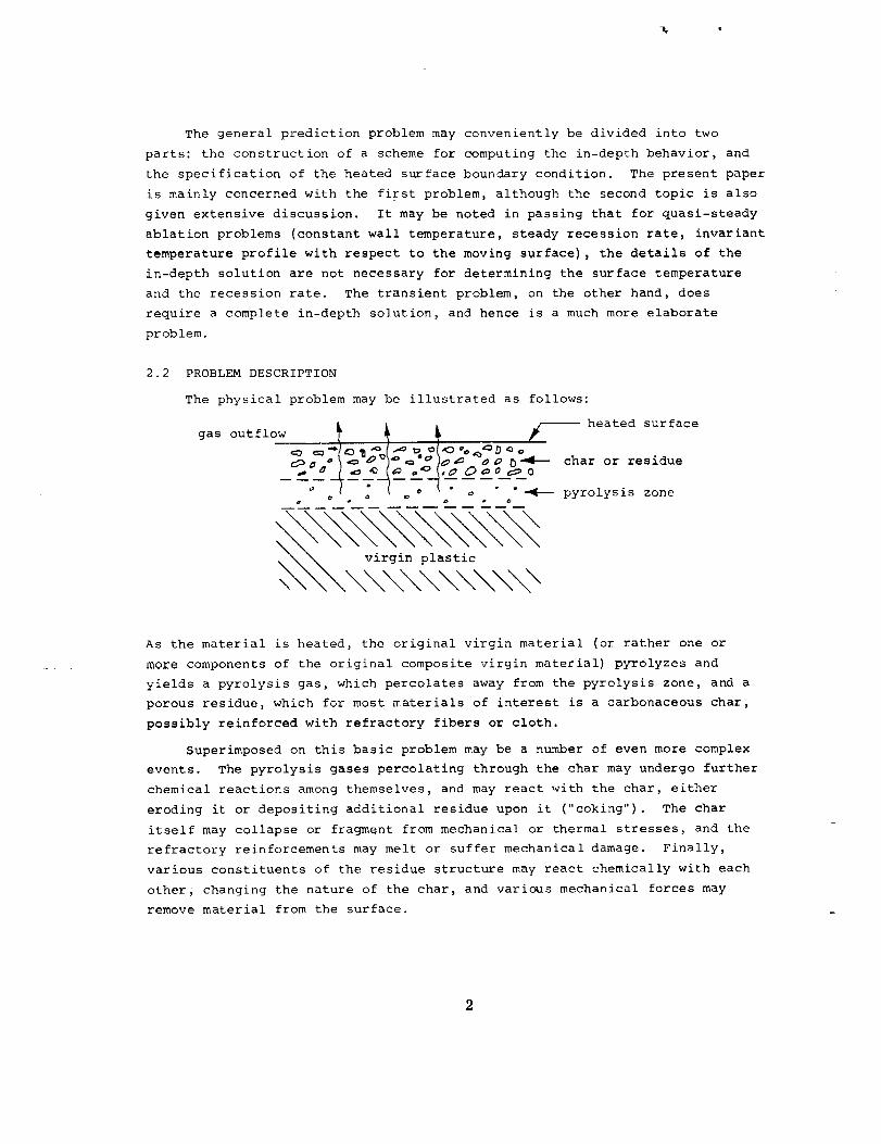
2.2 PROBLEM DESCRIPTION

The physical problem may be illustrated as follows:

gas outflow J !

o _

• _ _------ heated surface

_ o)Q_ oO 0_ char or residueo_I,o £9_o _ 0

--_--y'-_ _ - "_- pyrolysis zone

As the material is heated, the original virgin material (or rather one or

more components of the original composite virgin material) pyrolyzes and

yields a pyrolysis gas, which percolates away from the pyrolysis zone, and a

porous residue, which for most materials of interest is a carbonaceous char,

possibly reinforced with refractory fibers or cloth.

Superimposed on this basic problem may be a number of even more complex

events. The pyrolysis gases percolating through the char may undergo further

chemical reactions among themselves, and may react with the char, either

eroding it or depositing additional residue upon it ("coking"). The char

itself may collapse or fragment from mechanical or thermal stresses, and the

refractory reinforcements may melt or suffer mechanical damage. Finally,

various constituents of the residue structure may react chemically with each

other, changing the nature of the char, and various mechanical forces may

remove material from the surface.

Despite these complexities, it is found that the "simple physics"

described by

virgin plastic _ char + gas

underlies a wide range of problems of technical interest, and for a great

many materials, such as carbon phenolic, graphite phenolic, and wood,

constitute all the events of interest. Such events as coking, mechanical

erosion, melting, and subsurface reactions (other than pyrolysis) are less

common and generally characterize specific problems.

Therefore in any effort to compute the in-depth response of pyrolyzing

materials the first order of business is to characterize the heat conduction

and the primary pyrolysis reaction, which have useful generality. Particular

details of special char chemical systems can then be superimposed upon this

general computational scheme as required. The present effort has been

mostly devoted to the general conduction-pyrolysis problem. The numerical

details are described in Section 3.

2.3 PROBLEM HISTORY

In general terms, the in-depth calculation requires the solution of a

differential energy transport equation of the form (for one space dimension,

and neglecting gas flows for the moment)

k - pCp

plus an associated decomposition or charring kinetic relation

_- f(p,t)

This coupled pair of differential equations in general defies analytical

treatment and requires_ instead, some approximate technique of solution.

Perhaps the first general attack on this problem was published by Bamford,

Crank, and Malan in 1946 (Reference i). This paper presented a temperature-

implicit finite difference method, later elaborated in Reference 2, which

became known as the Crank-Nicolson method. The second paper also presented

two methods suitable for differential analyzer or analog computations.

Applications of ablating or sacrificial insulations for rocket nozzles

and for re-entry vehicle heat shields in the 1950's naturally stimulated a

great deal of development work on charring material predictive techniques.

References3 - 30provide a representative samplingof that part of the litera-ture which is aimedprimarily at the analysis of the in-depth responseofcharring materials. (A more complete bibliography may be found in Reference

31 .)

Many of these analyses, particularly References 9, 15, 18, 22, 23, 24,

27, and 28, were associated with the development of computer programs for in-

depth response computation. All of these programs treat the in-depth problem

in very much the same way, with only relatively unimportant variations in the

numerical formulation and the treatment of the pyrolysis kinetics.

The present computation scheme does not differ to any very great extent

from the best versions of earlier programs. It does feature a very great

fidelity to the observed physics of charring materials, a difference scheme

which rigorously conserves mass and energy, an economical implicit finite dif-

ference formulation, and the capability of handling general two-dimensional

geometries with the limitation of one-dimensional energy flow.

SECTION 3 _

ANALYSIS AND COMPUTATIONAL PROCEDURE FOR

CHARRING MATERIAL RESPONSE

3.1 PROBLEM FORMULATION

3.1.1 Introduction

Analysis of a complete transient charring material ablation problem

necessarily involves a computation of the internal thermal response of the

charring material. As discussed in Section 2 above, this computation consti-

tutes only a transient heat conduction calculation including the effects of

internal thermal decomposition with pyrolysis gas generation, coupled to an

appropriate set of boundary conditions. The sections below present the funda-

mental assumptions and equations invovled in the in-depth solution.

3.1.2 Basic Differential Equations

For the basic in-depth solution, it is assumed that thermal conduction

is one-dimensional; however, the cross-section area (perpendicular to the

conduction flux) is allowed to vary with depth in an arbitrary manner. This

corresponds to a thermal stream tube. Furthermore, it is assumed that any

pyrolysis gases formed are in thermal equilibrium with the char. For the

present discussion, it is assumed that the pyrolysis gases do not react chemi-

cally with the char in any way. Thus coking or further chemical erosion are

excluded. Theseeffects will be discussed in Section 3.1.4 below. Finally,any pyrolysis gas formedis assumedto pass immediately out through the char,

that is, it has zero residence time in the char. Cracking or other chemical

reactions involving only the pyrolysis gases may be simulated with an appro-

priate gas specific heat.

The one-dimensional energy differential equation for this problem is

readily formulated as

8 (phA) 8 ( ST) + 8 - (I)8--_ y = _ kA _ 8 _y (mghg) 8

where p is the density, k is the thermal conductivity,

enthalpy, and mg the local gas flow rate.

The conservation of mass equation is

A is area, h is

= A

5y )8 y

C2)

Evaluation of this expression requires a specification of the decomposition

rate 5p/50) A great amount of laboratory pyrolysis data, such as thatY

presented in Ref. 32, suggest that the decomposition rate may be taken as an

Arrhenius type of expression

-E/RT p - prlmap_@Y= -B e Po Po

(3)

and for even greater generality it has been found useful and sufficient to

consider up to three differently decomposing constituents (Ref. 32)

p = F(p A + pB ) + (I - F)PC (4)

where for example (PA + PB ) might be the density of resin (or analogous binder)

in the ablating material, PC would be the density of the reinforcement and

F the volume fraction of resin in the virgin plastic composite. Each density

PA' PB' and PC' may follow an independent decomposition equation of the type

of Eq. (3).

It is possible to handle the decomposition in other ways than by Eq. (3).

A popular simplification is to treat density as a function of temperature

only. An even more drastic simplification converts the virgin material to

complete char at one particular "charring temperature." Other techniques

specify some char thickness as a function of time, or of heating rate. All

of these simplifications are, of course, open to objection. Equation (3) is

not only the most realistic physically, but is usually easy to handle in com-

putation.

3.1.3 Boundary Conditions

Suitable boundary and initial conditions for the set of equations (i)

through (4) may be readily formulated. The boundary conditions at the front

and back faces of the ablating material are usually surface energy balances.

Of these, the front or "active" surface boundary condition is the most com-

plex. It is handled in slightly different ways depending on which boundary

layer treatment is being coupled to the in-depth reaponse program.

Basically, the surface energy balance may be pictured as

_qdiff _ q[_d I qradOut I (pv) whwF -- -- -- _ q*

_h _ hqcond c c gs g

where the indicated control volume is fixed to the receding surface. Energy

fluxes leaving the control volume include conduction into the material, radia-

tion away from the surface, energy in any flow of condensed phase material

such as liquid runoff, and gross blowing at the surface. Energy inputs to the

control volume include radiation in from the boundary layer and enthalpy fluxes

due to char and pyrolysis gas mass flow rates. The final input in the sketch

is denoted qdiff " It includes all diffusive energy fluxes from the gas

boundary layer. If the in-depth response computation is being coupled to an

exact boundary layer solution, the term qdiff will be available directly as

6

a single term (which is, of course, a complex function of many boundary layer

properties). If, on the other hand, the in-depth response is being coupled

to a simplified boundary layer scheme, such as a convective film coefficient

model, then the term qdiff has a rather complicated appearance. Section

5 b41ow contains a further discussion of this aspect of the total computation.

For the present, it suffices to note that computation of the surface

energy balance requires the following information from the in-depth solution:

a. the instantaneous pyrolysis gas rate delivered from in-depth to

the surface,g

b. a relation between the surface tmmperature and the rate of energy

conduction into the material, qcond

With these two pieces of information the surface energy balance then deter-

mines the char consumption rate mc and the surface temperature T w. It

will be useful to keep in mind that, from this point of view, the purpose of

the in-depth solution at any instant is to provide information about _g

and qcond (Tw)" In some circumstances, of course, it is of interest merely

to specify the heated surface temperature and recession rate. In this case

no surface energy balance is required.

It is usually of interest to have only one ablating surface. The back-

wall or non-ablating wall boundary condition may be modelled with a film

coefficient heat transfer equation.

3.2 FINITE DIFFERENCE DEVELOPMENT

3.2.1 Introduction

Section 3.1.2 above sets forth the governing differential equations whose

solution is required to define the interal response of the charring material.

As in many other problems, however, the differential equations cannot be

solved in general, and it is necessary instead to solve finite difference

equations*which model the differential equations, and the analyst hopes, re-

tain the same mathematical properties as the original differential equations.

A number of plausible difference equations can be proposed, and without the

benefit of actual experience it is generally impossible to select any particu-

lar differencing scheme as superior to any other. In the past few years a

*It is possible, of course, to use simpler schemes than finite difference

equations. Reference 33 is a sample of the several integral analysis

approaches which have been tried. Such techniques are usually of insuf-

ficient accuracy to be generally useful, however.

few general differencing principles havebeenmadereasonablyclear, however,so that the analyst is not completely in the dark. The following section

offers some background on this topic.

3.2.2 Differencinq Philosophy

This section sets down the general principles upon which the finite dif-

ferencing of the governing equations is based. These principles have proved

sound and useful, particularly for complex problems.

In common with all difference procedures, the area of interest (here,

the charring material) is divided into a number of small zones, each consid-

ered to be homogeneous. All derivatives in the governing differential equa-

tions are then replaced by some difference expression from zone to zone.

These zones, called nodes, thus provide the basic conceptual structure upon

which the differencing procedure is based.

The following principles of differencing and nodal sizing have been

followed in the programming work:

(i) The nodes have a fixed size. This avoids the slight additional com-

putation complexity of shrinking nodes, and more importantly, makes principle

(2) easier to satisy, in addition to preserving a useful nodal spacing through-

out the history of a given problem.

(2) Since the nodes are fixed in size, not all of them can be retained

if the surface of the material is receding due to chemical or mechanical

erosion. From time to time a node must be dropped, and experience shows that

it is much more preferable to drop nodes from the back (non-ablating) face

of the material rather than from the front face. See, for example, Ref. 34

for a discussion of this problem. This means that the nodal network is "tied

to the receding surface," and that material appears to be flowing through the

nodes. This involves a transformation of differential equations (i) and (2)

to a moving coordinate system and somewhat complicates the algebra of the

difference equations modelled on these differential equations. Disposing

of nodes from the front surface, however, often leads to undesirable oscil-

lations.

(3) The difference forms of derivatives are kept simple and are formed

so as to provide a direct physical analog of the differential event leading

to the derivative. This approach may be contrasted to those approaches

which seek elaborate difference approximations to derivative expressions.

Experience shows that the scheme advocated here, while sometimes at a minor

disadvantage in accuracy, greatly simplifies the attainment of a major objec-

tive: a difference scheme which conserves energy and mass. Many of the more

8

elaborate difference schemes fail to meet these "simple" but crucial conser-

vation criteria, and hence frequently converge to erroneous or spurious solu-

tions.

(4) The difference equation for energy is formulated in such a way

that it reduces to the difference equation for mass conservation when tem-

peratures and enthalpies are uniform. Any lack of consistency between the

energy and mass equations complicates, and may entirely defeat, convergence

to a meaningful result.

(5) The difference energy equations are written to be "implicit" in

temperature. That is, all temperatures appearing are taken to be "new"

unknown temperatures applicable at the end of the current time step. It is

well established that implicit procedures are generally more economical than

explicit procedures, at least for the majority of ablation problems of inter-

est in the current work.

(6) In constrast to point (5), the decomposition relations are written

as "explicit" in temperature. To implicitize temperature in these highly non-

linear equations necessarily involves either a time-consuming iteration pro-

c6dure or an elaborate linearization, which is not necessary for most

materials.

(7) Since experience has shown that material decomposition rates are

strongly dependent on temperature, it is highly desirable to perform the mass

balance operations in a different, tighter network than that used for the

energy balance equations. For greatest generality and utility, the number

of these mass balance "nodelets" per energy balance "node" should be freely

selectable.

3.2.3 Transformation of Differential Equations

3.2.3.1 General Remarks

Solution of the in-depth response will be by difference equations. The

most convenient finite difference equations governing particular physical

phenomena may often be derived directly from considering a control volume

of finite (not infinitesimal) extent. Such is the case, for example, when

characterizing the thermochemical response of charring materials having con-

stant cross-sectional area (the flat plate case). Far the present problem,

however, where the cross-sectional area may be an arbitrary function of dis-

tance below the surface, substantial s implifications_may be realized if the

equations are first considered in differential form. Specifically, differ-

ences in cross-sectional area with respect to space and time appear in the

difference equations derived from the finite control volumeapproach. Theneglect of these terms is difficult to rationalize from the difference equa-tions; however, if the differential equation is employed,these terms maybe demonstratedto vanish identically. The resulting differential equationsmaythen be expandedinto finite difference form yielding a set of finitedifference equations substantially simpler than those derived directly fromanalyzing a finite control volume. Thedifferential equations are consideredfirst, and subsequentlyexpandedto finite difference form.

As discussed in Section 3.2.2 above, it is deemedconvenient to basethe difference formulation on a nodal network fixed to the heated surface.Since this surface will be receding, material will appearto flow into andout of the nodes. Thedifferential equations presentedas Eqs.(i) and (2)require transformation to a movingcoordinate systemto include this aspectof the problemand to provide the proper model for differencing. Themassequation is treated first, in Section 3.2.3.3. Discussion of the energyequation follows. First, however,someobservations about the geometryarerequired.

3.2.3.2 GeometricalConsiderations

The generalized geometrybeing considered and the coordinate systemtobe employedfor the subsequentdifferential and finite difference equationsare shownin Figure I.

Geometrical considerations are introduced to the subsequentequations inthe form of specification of the cross-sectional area as a function of dis-tance below the initial surface, A = A(y). In the event consideration of

certain special geometries is desired, for example, cylindrically symmetric

(A _ r°), these functional relationships may be simply obtained to yield

the cross-sectional area as a function of distance below the initial surface.

It is important to observe that the origin of the y coordinate ks

fixed in space (relative, say, to the back wall). Thus a control volume

at "constant y" contains a fixed, identified piece of material. The origin

of the x-coordinate, on the other hand, is tied to the receding heated sur-

face.

3.2.3.3 Conservation of Mass In Moving Coordinate System

Decomposition of the ablation material in-depth is characterized by an

irreversible reaction of the following form:

plastic -_ char + gas

I0

Initially the ablation material is considered to be all plastic, and after

decomposition it is all char. Intermediate states need not be considered

until later. The mass conservation equation is written neglecting the mass

of the gas at any point as being small compared to the mass of solid material

and assuming that the transit time of the gas from the point of decomposition

to the heated surface is small. Within these constraints the mass conserva-

tion equation may be written

_y /_ _ (pA)y = A + p(5)

where the subscripts indicate variables held constant when performing partial

differentiation, but A = A(y) alone, so the term

and the mass conservation equation becomes

_Y /O = A

(6)

(7)

given earlier as Eq. (2). In the above equation, mg, represents the mass

flow rate of gas past a point, and its derivative with respect to distance

is seen to equal the gas generation rate. The total gas flow rate passing

a point is obtained by integration of Eq. (7)

_g = - A dy

(8)

The material density, p, and density change rate resulting from decomposition

(_p/_)y, is obtained from considering the material formulation. The virgin

plastic may consist of up to three decomposible constituents, and the density

of the composite is given by Eq. (4)

p _, F(p A + lOB) + (i -F) PC (4)

11

where (JA + i_B) is the density of the resin, Pc is the density of the rein-

forcement, and F is the volume fraction of resin in the virgin plastic com-

posite. The division of resin into A and B components is a consequence of

the experimentally observed two-stage decomposition process of phenolic resin.

The rate of change of density resulting from decomposition is given by differ-

entiating equation (4) with respect to time at constant y.

y k7 + \ o /y(9)

where decomposition of each constituent is given by a rate equation of the

Arrhenius form.

_?i_ -Ei/RT __Pi -_ Pri_ mi

= i P°i k P°i /_--jy - k e for i = A,B_C (10)

It is now necessary to relate these density changes at constant y to

the density changes at constant x since we plan to work with the x co-

ordinate system. At any instant in time the density may be expressed purely

as a function of spatial position and time, P = p(Y,0)- Then

d_ - _y

(ll)

Differentiating with respect to time at constant x yields

From Figure 1 the

recession

(12)

x and y coordinates are related to the amount of surface

fr0m which

y = S + x (13)

dS

12

where the surface recession rate_ S, is written as an absolute derivative since

S = S(_) alone. Substituting this expression into the above equation yields

(15)

which, with Equations (9) and (10), represents the desired form of the mass

conservation equation.

3.2.3.4 Conservation of Energy in Moving Coordinate System

The energy equation is written first with respect to a spatially fixed

coordinate system. For this purpose_ the following functional relationships

are presumed:

h = h(T,_)

T = T(y,e)

(= _(y,_)

A = A(y)

s = s(e)

therefore

h " h(y,8)

The differential equation governing the conservation of energy within the char-

ring material is obtained by considering the control volume in Figure 1 and

equating the net energy transfer rate to the rate of energy change, The re-

sulting equation was cited as Equation (i)

storage conduction convection

For the numerical solution it is convenient to consider a coordinate system

fixed to the receding surface, as discussed above. To transform the above

differential equation, which is written for a point, y = constant, to an

equation written for the moving coordinate system, x = constant, the storage

term in Eq. (i) may be related to its counterpart in the moving coordinate

system by expanding the energy change employing the chain rule:

13

_hA _ phA(y,e)

Differentiating partially with respect to time at constant x yields:

_0 (phA)x _" _ (0ha)0 ÷ _ (phA)y (16)

Introducing Equation (14) and rearranging obtains

(phAly = _ (phA) x - S _y (phA) 0 (17)

Substition of Equation (19) into Equation (i) with the observation that partial

differentiation with respect to x or y at constant time is equivalent, re-

sults in the transformed energy equation

I II III IV

The above terms will be considered separately below.

Term I

It is convenient to express the enthalpy change rate in terms of tempera-

ture and density change rates. For that purpose it is necessary to set down

some specific model for computing enthalpy. It is deemed convenient and

fairly reasonable to imagine that partially pyrolyzed material may be regarded,

for the purpose of computing material properties, as a mixture of pure char

and pure plastic. A convenient quantity for algebraic manipulation is then

¢p, the volume fraction of imagined undecomposed material in the control vol-

ume. For undecomposed material ep is i; for pure char _p = 0, and for

intermediate states of decomposition it may be anywhere in between. Then the

density may be written

p = £ppp + (i - £p)Pc (20)

14

The total enthalpy per unit volume may be written as the mass weighted aver-

age of the enthalpy of the parts

(21)_h = eppphp + (i - 6p)Pch c

where

T

-- h° + / Chp P PP

o

dT (22)

and

T

= h° + / Chc c Pco

dT (23)

Differentiating Equation (21) obtains

___ _¢p _ _hc30 (_h) = pphp _ + ppEp Be + Pc

_ep _h- Pchc _9 - epPc _ (24)

Differentiating Equations (22) and (23), and noting that the char and plastic

heats of formation are constant, we have

_h _X_hp _T _ = C

_e - Cpp _ and _e Pc _e

(25)

Differentiation of Equation (20) results in

3e Pp - Pc _e(26)

Substitution of Equations (25) and (26) into (24) yields the desired rela-

tion between enthalpy change rate, temperature change rate, and decomposition

rate

_0 (Ph)x = + (27)k, 9p Pc pCp

where

+ (i - ep)pCp ppepCpp PcCpc

(28)

15

The specific heat, Cp'

and virgin plastic parts, and, as such, it represents the specific heat of

the material evaluated in the absence of chemical reactions.

Utilizing the above, and Equation (12), Term I in the differential

Equation (ii) may be written as follows:

+be (phA)x " ph + A h PP Pc pCp

Term II

is the mass weighted average specific heat of the char

Term II in Equation (18) will not require any modification.

Term III

For Term III we have

Now A = A(y)

A = A(x,8)

= _A}8 + SA _ (ph) (30)

alone, but y = x + S, and S = S(_) alone, so we may write

dA I" _X

Differentiating partially with respect to time at constant y

4But, since A = A(y) alone, _A/_8) = 0. Also, since y = x + S

Y

(31)

Combining the above results in

obtains

(32]

(33)

ax}e = _}x (34)

i Substituting Equation (34) into (30) yields a new expression for Term III.

_x (phA)_ = ph _}x + SA _x (Ph)8 (35)

16

Term IV

Term IV may be written

_x " _q-/e + hg (36)

Since differentiation with respect to x and y at constant time are equi-

valent, substitution of the mass conservation Equation (7) into the above

gives

_-- (mghg) = mg + A (37)

Substitution of Equations (25), (35), and (37) into the energy differential

Equation (18) yields

)ya F_-/0 + hg _0 (38)

where

_ pphp - Pch

Pp - Pc

The terms in Equation (38) represent, from left to right, the sensible

energy accumulation, the net conduction, the chemical energy accumulation,

net energy convected as a consequence of coordinate motion, net energy con-

vected by the pyrolysis gases passing through, and the energy convected away

by pyrolysis gases generated at the point. All terms are evaluated per unit

volume. Note that the pyrolysis gas flow rate past a point, mg, is the total

flow rate (see Equation(8)) and must be divided by area to be on the same

basis as the other terms in the equation.

The finite difference formulation of the above derived differential

equations for mass conservation (Equations (9), (i0) and (15)) and energy

conseration (Equation (38)) are presented in the two succeeding sections.

Before those types are considered, however, it is of passing interest to

note that Equation (38) which turns out to be a convenient form for machine

treatment, can be cast into more appealing form. Some tedious but straight-

forward algebra, the details of which are given in Appendix D. yields

17

I c39pCp_ x = _ kA_xe (hg Y e e

With the energy equation in this form, each term has a more readily perceiv-

able physical significance.

As a final note, it may be observed that equations (9), (i0), and (15)

for mass conservation and Equation (38) for energy conservation cannot be

used as models for the last ablating node, which is a shrinking as opposed

to a drifting node. It will prove not necessary to have differential equa-

tions for this node; the difference equations may be obtained directly.

3.2.4 Difference Forms

3.2.4.1 Mass Equation

3.2.4.1.1 Nodes other than the first or last

Experience with the finite difference solution of the preceding differen-

tial equations has shown that, generally, a much finer definition of the

space derivative is required for an accurate solution of the mass conserva-

tion equation than for the energy conservation equation. This is the case

because, for most material-boundary condition combinations of interest, the

density profile through the material is much steeper than the corresponding

temperature profile. As a result, the finite difference spatial grid size

selected to represent the mass conservation solution is much smaller than that

selected to represent the energy equation solution. Space derivatives for

the energy equation solution are obtained by considering an array of nodes,

while space derivatives for the mass conservation equations are based upon

consideration of a number of nodelets in each node. A schematic representa-

tion of the spatial grid is shown in Figure 2 where it is seen that each

node (n) remains a fixed distance below the surface (Xn) and has a constant

thickness, 6 n. The last node in the ablation material (n = NL) is the one

exception to this in that it will continually shrink as surface recession

proceeds until it vanishes at which point the next to last node becomes the

new last node. Special treatment afforded the last ablating node to include

consideration of the shrinking process is described subsequently, in Section

3.2.4.1.3. Referring to FigUre 2 it is noted that each node is subdivided

into J nodelets, each designated n where j ranges from 1 to J for3

each node. The mass balance equation is satisfied for each nodelet in the

following development.

18

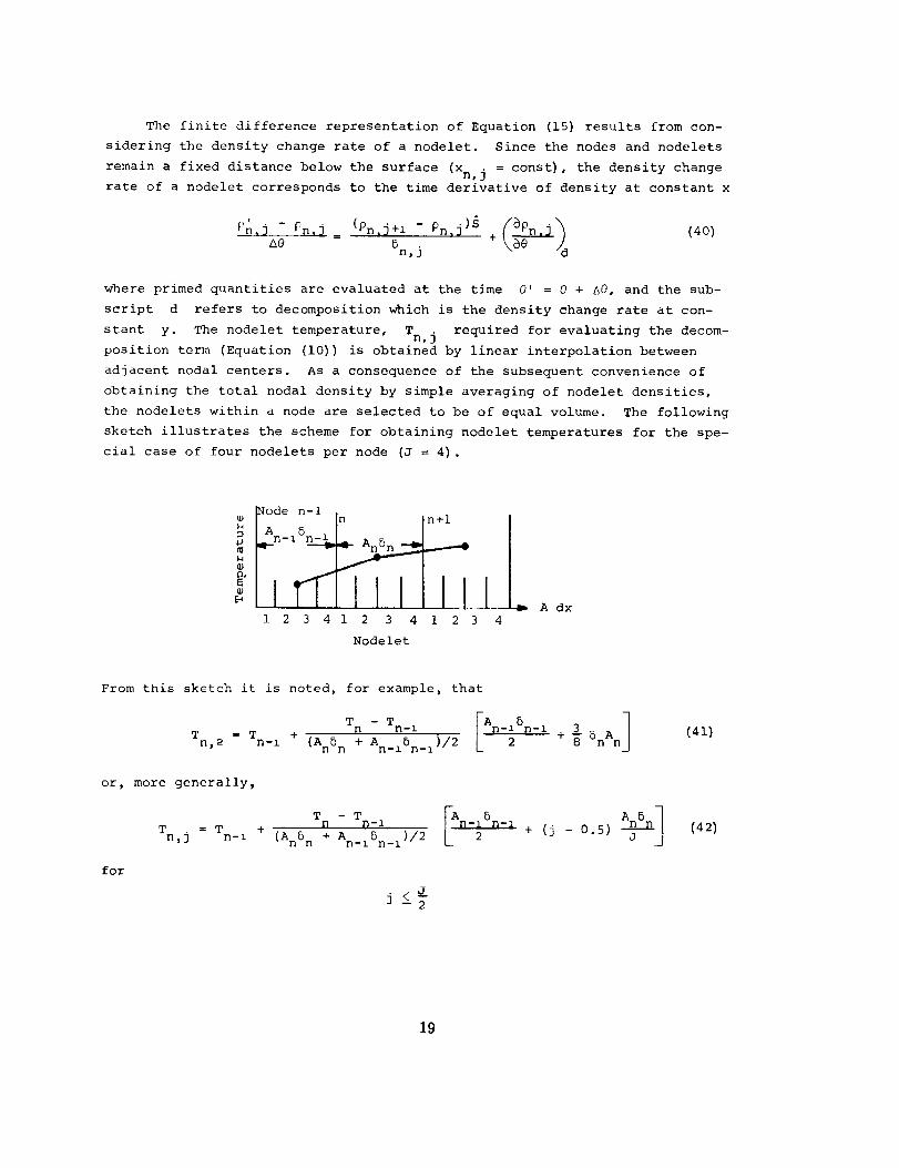
The finite difference representation of Equation (15) results from con-

sidering the density change rate of a nodelet. Since the nodes and nodelets

remain a fixed distance below the surface (Xn, j = const), the density change

rate of a nodelet corresponds to the time derivative of density at constant x

In_3 - ?n,j (Pn,_ +l - Pn,_ )_ /_Pn__ (40)= +

Ae 5n, j _0 /d

where primed quantities are evaluated at the time e' = e + A0, and the sub-

script d refers to decomposition which is the density change rate at con-

stant y. The nodelet temperature, Tn, j required for evaluating the decom-

position term (Equation (i0)) is obtained by linear interpolation between

adjacent nodal centers. As a consequence of the subsequent convenience of

obtaining the total nodal density by simple averaging of nodelet densities,

the nodelets within a node are selected to be of equal volume. The following

sketch illustrates the scheme for obtaining nodelet temperatures for the spe-

cial case of four nodelets per node (J = 4).

_ode n-i"n n+l

n-i

|I[7111I1111°........... v_

1 2 3 4 1 2 3 4 1 2 3 4

Nodelet

A dx

From this sketch it is noted, for example, that

Tn,2

T - T

= T + n n -l

n-i (An_ n + An_l_n_l)/2AnrA_D-I 3 12 + 8 6nAn

or, more generally,

T = T +n,j n-i

T - T

(An5 n + An_lSn_l)/2IA AnBn-_ 5n-I + (j- 0.5)_-_

for

(41)

(42)

19

and

for

Tn_j = T + Tn+l - T D F qm(j _ 0.5) _ 0.5] A 5 (43)n (An+ibn+ 1 + AnSn)/2 J n n

J

J > _

The nodelet density change rate of constituent i resulting from decom-

position is obtained from Equation (10) utilizing the above nodelet tempera-

tures.

m.

%Pi,n_j = - k.e Ei/RTn' J ?i,n,j Pr 1 (44)

_ D l Po i po i

It is noted that the decomposition rate depends upon two quantities, Pi,n,j

and Tn, j, which may vary during a time interval (4@). If temperature and

density variations during a time interval are large enough to significantly

effect the decomposition rate, either the time step size must be reduced or

a temperature and density more representative of the average over the time

interval should be employed in order to obtain a stable solution. Most gen-

erally, for problems of practical interest, a nodelet undergoing decomposi-

tion is experiencing a density decrease and a temperature increase. Equation

(44) suggests that using the density, 0i,n,j, at the beginning of the time

interval will result in too large a decomposition rate while using the tem-

perature, Tn, j, at the beginning of the time interval will result in too

small a decomposition rate, for most cases of interest. Since instabilities

are usually associated with too large rather than too small a change rate,

it is appropriate to consider an implicit treatment of the density while

treating the temperature in an explicit manner, at least as a first try.

Such an explicit treatment of the temperature is possible because the decom-

position energy of organic constituents is small and, as such, the coupling

between energy and mass conservation equations is weak for nodes in the de-

composition region.

An effective "implicit" treatment of the density in the decomposition

equation may be readily obtained from direct integration of Equation (44)

holding the temperature fixed over the time interval. The following results:

2O

) (....)5Pi,n,j = Pi,n, j _0Pl,n, 3

_O D y

l-m i 1 - m i -Ei/RTn' J 1_ri - Pi,n,j + (Pi,n,j - Pri ) m.-Y kie be JPoi i

1

-l-m.l

be

(45)

for m. _ I, and1

(46)

for m. = 11

These implicit relations yield a much more stable solution than is ob-

tained with Equation (44) treating the density explicitly.* The overall

density change rate of a nodelet resulting from decomposition is obtained by

summing the decomposition rates of each constituent via Equation (i0) . The

total nodelet density change rate over a time interval due to decomposition

and coordinate system motion is obtained from Equation (40).

Since the energy equation is solved on the basis of full nodes rather

than nodelets it is necessary to evaluate the total nodal density change

rate. For an even number of equally sized nodelets in each node, 6n, j • An, j

constant, that is, such that each nodelet has the same volume, the total nodal

density change is the arithmetic average of the density changes of all of the

nodelets:

J

3=i

J

_n j=l

*Calculational results utilizing both integrated and explicit density depen-

dence in the decomposition equation are presented subsequently in Appendix B.

Use of the integrated form was suggested in Reference i, but this device

appears to have been largely overlooked in more recent work.

21

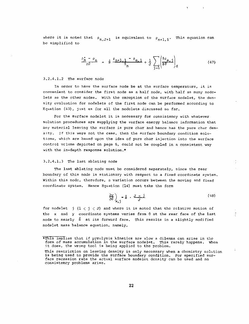
where it is noted that Pn,J+l is equivalent to

be simplified to

Pn+l,l" This equation can

°n°nAe = _ Pn+l,l - Pn,l +

6n j =i \ /d

3.2.4.1.2 The surface node

In order to have the surface node be at the surface temperature, it is

convenient to consider the first node as a half node, with half as many node-

lets as the other nodes. With the exception of the surface nodelet, the den-

sity evaluation for nodelets of the first node can be performed according to

Equation (43), just as for all the nodelets discussed so far.

For the surface nodelet it is necessary for consistency with whatever

solution procedures are supplying the surface energy balance information that

any material leaving the surface is pure char and hence has the pure char den-

sity. If this were not the case, then the surface boundary condition solu-

tions, which are based upon the idea of pure char injection into the surface

control volume depicted on page 6, could not be coupled in a consistent way

with the in-depth response solution.*

3.2.4.1.3 The last ablating node

The last ablating node must be considered separately, since the rear

boundary of this node is stationary with respect to a fixed coordinate system.

Within this node, therefore, a variation occurs between the moving and fixed

coordinate system. Hence Equation (14) must take the form

_ =_. J-____j (48)

_/x ,j J

for nodelet j (I < j < J) and where it is noted that the relative motion of

the x and y coordinate systems varies from 0 at the rear face of the last

node to nearly S at its forward face. This results in a slightly modified

nodelet mass balance equation, namely,

*This implies that if pyrolysis kinetics are slow a dilemma can arise in the

form of mass accumulation in the surface nodelet. This rarely happens. When

it does, the wrong tool is being applied to the problem.

This restriction on leaving density is only necessary when a chemistry solution

is being used to provide the surface boundary condition. For specified sur-

face recession rate the actual surface nodelet density can be used and no

consistency problems arise.

22

dPN-J __d + -_ J - Jde = 5N, j J (PN,j+z - PN,j )

(49)

The total density change of the last node will then be the sum of the density

changes of each of the nodelets or

J J

•Z Jde : J _e /d + JSN - (PN,j+I - PN,j

j:z j=z

J

j:z

(50)

3.2.4.2 Energy Equation

3.2.4.2.1 Nodes other than the first or last

A" finite difference representation of Equation (38) can be formulated in

a variety of ways. As with the mass equation, however, every effort will be

made here to preserve a correspondence with a finite nodal energy balance. For

example, the total enthalpy change rate given by Equation (27),

_0 (Ph)x : pCp

represents the nodal enthalpy change resulting from a change in density and

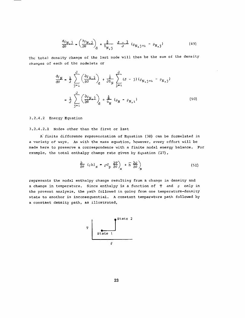
a change in temperature. Since enthalpy is a function of T and p only in

the present analysis, the path followed in going from one temperature-density

state to another is inconsequential. A constant temperature path followed by

a constant density path, as illustrated,

State 1

State 2

T

23

yields the following interpretation of the two terms on the right side of

Equation (51)

(52)

where h is evaluated at the initial temperature, and p'_ is evaluated

at %he final density and initial temperature. To be precise CD should be

evaluated at some mean temperature as well as at the terminal density, but

otherwise the relation is exact since _ is constant at constant temperature

and V is constant along the second segment of the selected path.

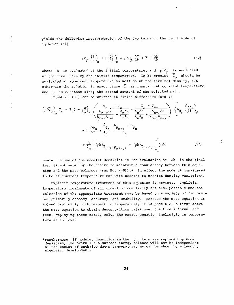
Equation (38) can be written in finite difference form as

_"_'P)n(T_ - T n) - 5_ n _5n_l/2 5n/2 8n/2 5n+1/2 '_+ gn _ _'_-"_/d

knAn + _-_n-iAn-i + k--_n kn+z n+J

h hA_

+ gn+l %A 5n n

+ 5_-- [(Ph)Tn+l _ Pn+l _ 1 - (Ph)Tn' Pn J> A0n , (53)

where the use of the nodelet densities in the evaluation of oh in the final

term is motivated by the desire to maintain a consistency between this equa-

tion and the mass balances (see Eq. (40)).* In effect the node is considered

to be at constant temperature but with nodelet to nodelet density variations.

Explicit temperature treatment of this equation is obvious. Implicit

temperature treatments of all orders of complexity are also possible and the

selection of the appropriate treatment must be based on a variety of factors -

but primarily economy, accuracy, and stability. Because the mass equation is

solved explicitly with respect to temperature, it is possible to first solve

the mass equation to obtain decomposition rates over the time interval and

then, employing these rates, solve the energy equation implicitly in tempera-

ture as follows:

*Furthermore, if nodelet densities in the ph term are replaced by node

densities, the overall sub-surface energy balance will not be independent

of the choice of enthalpy datum temperature, as can be shown by a lengthy

algebraic development.

24

Ik T' - T' T' - T' k

( ) Ae _-_ P _ n 5_ +I/2 )[_'C (Tn - Tn) - _ A' 5n_1/2 _n/2 5n/2

P n n n A' + k A' k A' + 'n-i n-i n n n n kn+lAn+i/

iI h _hg_ Tn) 1 <>_d %

/hh+_T /n (Tn+ l - Tn+ l) - hmgn gn+1 +1 gn

_-n n

TnJ

+ (_h)n+l i + pCp n -Tn+1) -n * n+l ,i

- <pCp_n,l(T n - Tn)IIA0

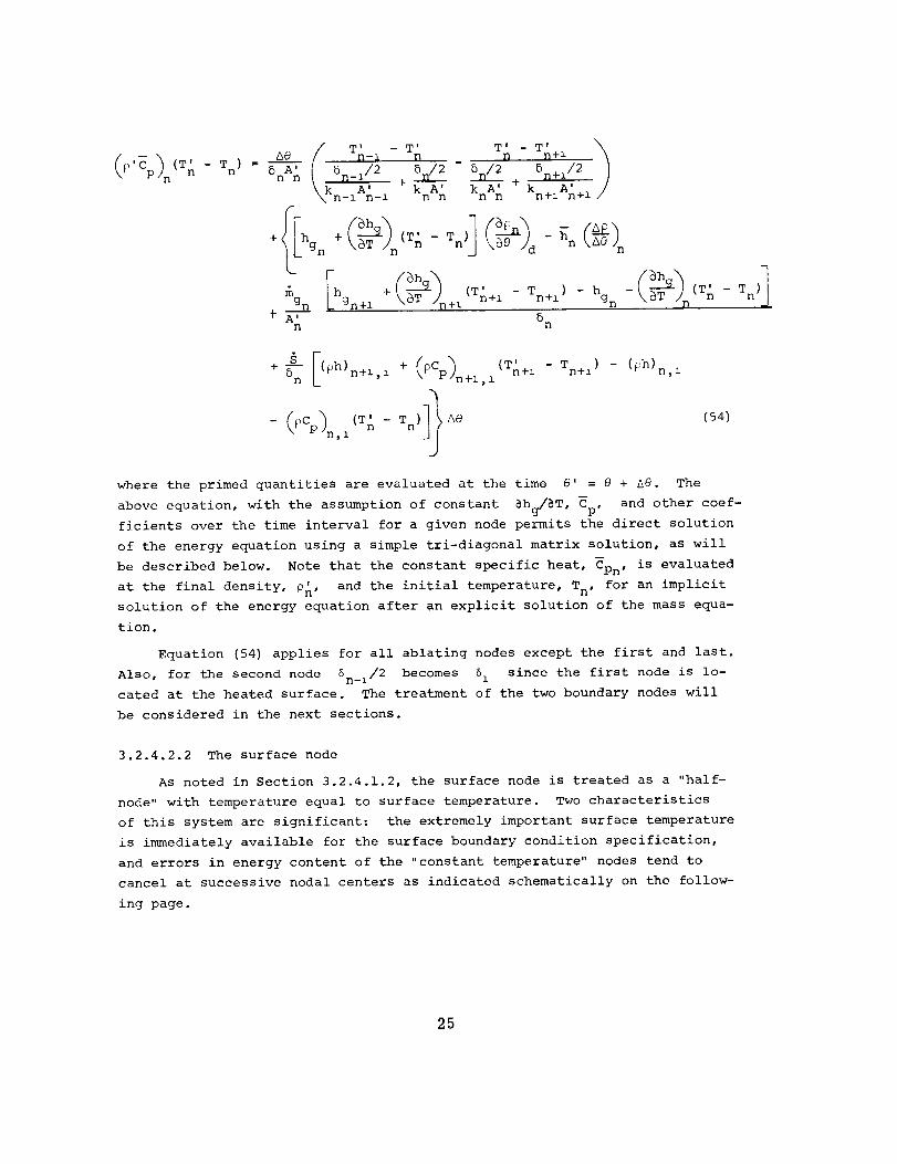
(54)

where the primed quantities are evaluated at the time 8' = 8 + &8. The

above equation, with the assumption of constant _h_T, Cp, and other coef-

ficients over the time interval for a given node permits the direct solution

of the energy equation using a simple tri-diagonal matrix solution, as will

be described below. Note that the constant specific heat, Cpn, is evaluated

!

at the final density, Pn' and the initial temperature, T n, for an implicit

solution of the energy equation after an explicit solution of the mass equa-

tion.

Equation (54) applies for all ablating nodes except the first and last.

Also, for the second node 6n_i/2 becomes 61 since the first node is lo-

cated at the heated surface. The treatment of the two boundary nodes will

be considered in the next sections.

3.2.4.2.2 The surface node

As noted in Section 3.2.4.1.2, the surface node is treated as a "half-

node" with temperature equal to surface temperature. Two characteristics

of this system are significant: the extremely important surface temperature

is immediately available for the surface boundary condition specification,

and errors in energy content of the "constant temperature" nodes tend to

cancel at successive nodal centers as indicated schematically on the follow-

ing page.

25

i I

I

z ix',. i

"_ "F-

_I I _ ' "4, I I I

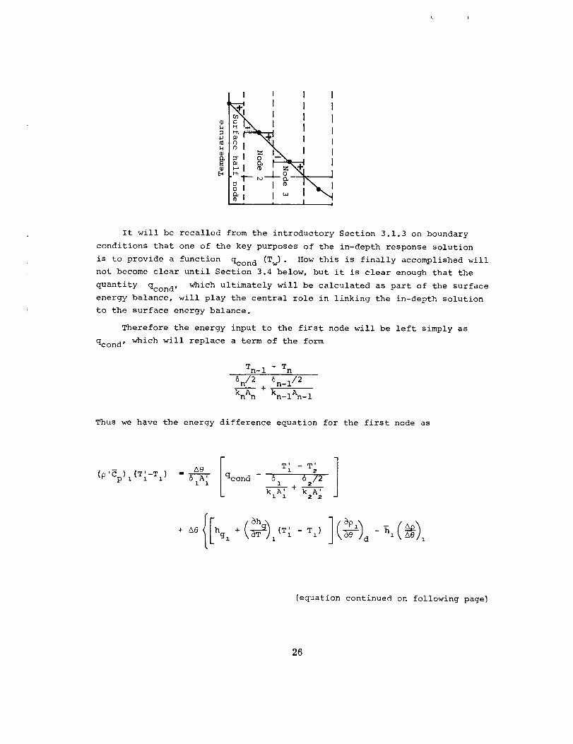
It will be recalled from the introductory Section 3.1.3 on boundary

conditions that one of the key purposes of the in-depth response solution

is to provide a function qcond (Tw)" How this is finally accomplished will

not become clear until Section 3.4 below, but it is clear enough that the

quantity qcond' which ultimately will be calculated as part of the surface

energy balance, will play the central role in linking the in-depth solution

to the surface energy balance.

Therefore the energy input to the first node will be left simply as

qcond" which will replace a term of the form

Tn_ I - T n

6n/2 6n_i/_+

knAn kn_iAn_ 1

Thus we have the energy difference equation for the first node as

'Cp) = AeA_----T(P i (T'I-TI) 61 I

T _ - T l

1 2

qcond - &1 62/2

k A' k A'i i 2 2

(T'I TI) ] / tDI" -

(equation continued on following page_

26

(equation continued from preceding page)

mgl lhg2 - - hgl - -T_ (T2 T 2) (T; TI) I

+ --

A' 61 i

+ _ (Ph)2 + (_cp)_,_(T_- T) - (_h)_ - (pCp)_(T"T) I}

(55)

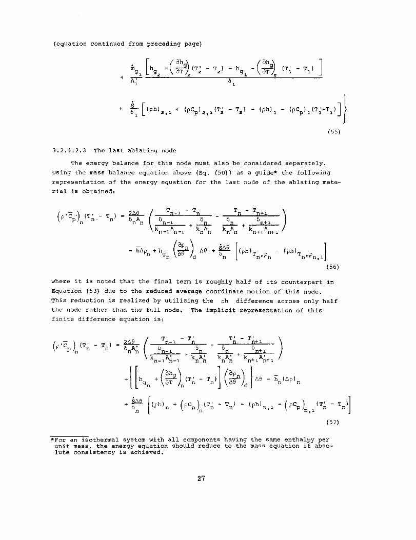
3.2.4.2.3 The last ablating node

The energy balance for this node must also be considered separately.

Using the mass balance equation above (Eq. (50)) as a guide* the following

representation of the energy equation for the last node of the ablating mate-

rial is obtained:

, (T n Tn ) 2_@ _ TD._I - T[_

\ kn-iAn -l khAn

_ TN - TD+ i

5n 5D+_ JknAn+ kn+iAn+ I

- hAPn + hg n \_8 /d + _ (Ph)Tn'Pn Pn,1

(56)

where it is noted that the final term is roughly half of its counterpart in

Equation (53) due to the reduced average coordinate motion of this node.

This reduction is realized by utilizing the ph difference across only half

the node rather than the full node. The implicit representation of this

finite difference equation is:

I ' ' T' - T' >TX]-I - Tn n n+l( %1o B 5

_ ' (Tn _n- l ___D_ __]l_ 5n+ 1

k A' + A' +k A' k kn+IA'+inn-i n-i n n n n

+ 5A_-[(_'h)n + (pCp)n (Tn -Tn)n - (Ph)n'" - (pCp)n,I

*For an isothermal system with all components having the same enthalpy per

unit mass, the energy equation should reduce to the mass equation if abso-

lute consistency is achieved.

27

with the assumption of constant coefficients this equation will also fall

within the framework of the tri-diagonal matrix solution to be discussed

below.

The nodelet density in the "leaving" ph term of Equations (56) and (57)

parallels the nodelet density usage in the mass equation (50). The "entering"

ph term retains the nodal density. If this procedure is not followed, a

lengthy algebraic development shows that the overall in-depth energy solution

will not be independent of the choice of enthalpy datum state.

3.2.4.2.4 Back-up nodes

Energy equations for the back-up nodes are the same as Equation (54) and

(57) without the decomposition and convection terms, since the nodal structure

only moves in the ablating material. The back-up nodal structure remains

fixed.

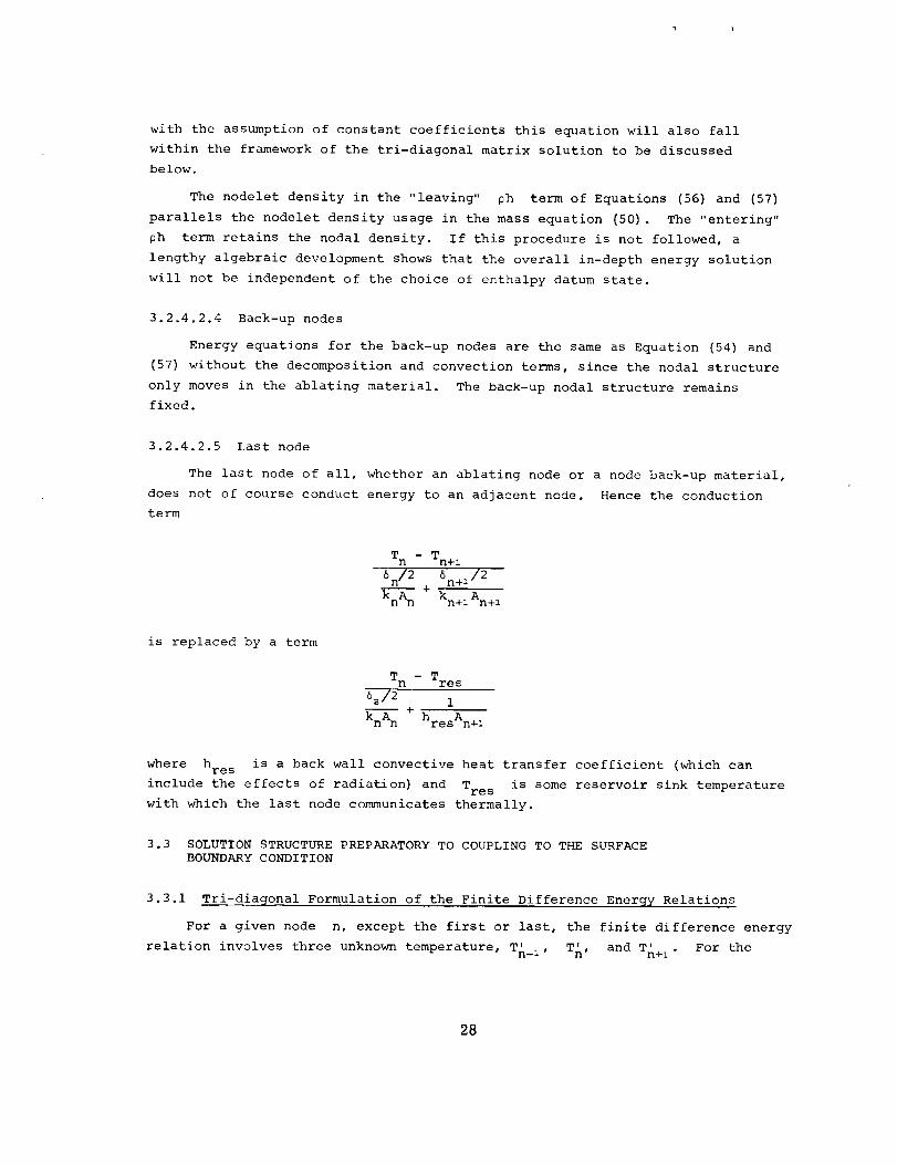
3.2.4.2.5 Last node

The last node of all, whether an ablating node or a node back-up material,

does not of course conduct energy to an adjacent node. Hence the conduction

term

T n - Tn+ i

6n/2 6n+i/2

+ kn+iAn+ i

is replaced by a term

T - Tn res

6_/2 1-- +

knAn hresAn+ i

where hre s is a back wall convective heat transfer coefficient (which can

include the effects of radiation) and Tre s is some reservoir sink temperature

with which the last node communicates thermally.

3.3 SOLUTION STRUCTURE PREPARATORY TO COUPLING TO THE SURFACE

BOUNDARY CONDITION

3.3.1 Tri-dia_onal Formulation of the Finite Difference Energy Relations

For a given node n, except the first or last, the finite difference energy

relation involves three unknown temperature, T'n_i, Tn" and T'n+i " For the

28

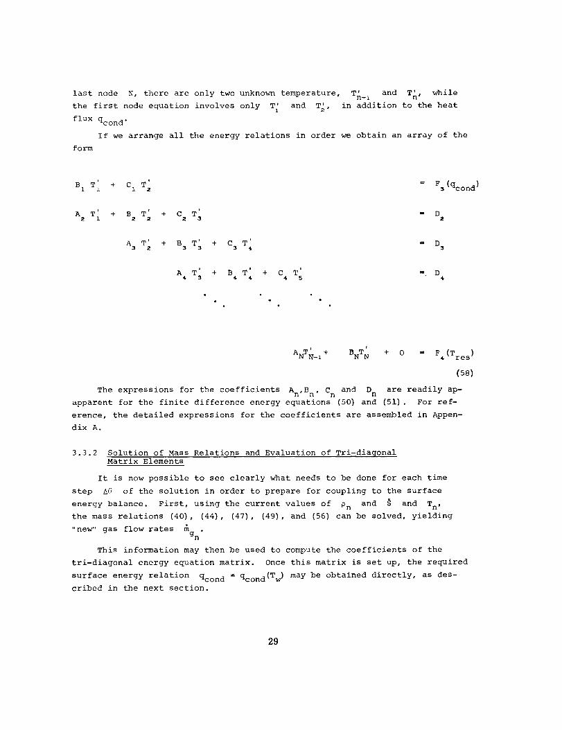
last node N, there are only two unknown temperature, T'n_l and Tn,' while

the first node equation involves only T' and T' in addition to the heatI 2'

flux qcond"

If we arrange all the energy relations in order we obtain an array of the

form

. , = F3(qcon d)B I T l + C l T

l i iA T + B T + C T = D

2 1 2 2 2 3 2

+ B T + C 3 T'A3 T2 3 4 3

A T' + B T' + C T' = D3 4 4 4 5 4

I!

NTN * * 0 -A -i BNTN F4 (Tre s )

(58)

and D are readily ap-The expressions for the coefficients An'Bn' Cn n

apparent for the finite difference energy equations (50) and (51). For ref-

erence, the detailed expressions for the coefficients are assembled in Appen-

dix A.

3.3.2 Solution of Mass Relations and Evaluation of Tri-diaqonal

Matrix Elements

It is now possible to see clearly what needs to be done for each time

step be of the solution in order to prepare for coupling to the surface

energy balance. First, using the current values of Pn and _ and T n,

the mass relations (40), (44), (47), (49), and (56) can be solved, yielding

"new" gas flow ratesgn"

This information may then be used to compute the coefficients of the

tri-diagonal energy equation matrix. Once this matrix is set up, the required

surface energy relation qcond = qcond(Tw ) may be obtained directly, as des-

cribed in the next section.

29

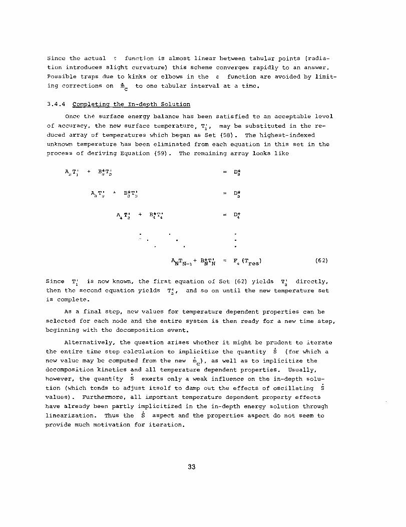
3.3.3 Reduction of Tri-diaqonal Matrix to Surface Energy Relation

Referring to the array of in-depth energy equations set down symbolically

as Set (58) in Section 3.3.1 above, it may be seen that, beginning with the

last node, the highest-indexed unknown temperature may be eliminated from

each equation of Set (58) in turn. (This is the standard first step in the

routine reduction of a tri-diagonal matrix.) Of the resulting simpler set of

equations (shown as Set (62) below and discussed at that time) only the top-

most is of immediate interest. It may be arranged as

qcond = F 5 (T_) (59)

where F s is a simple linear relation. It will be noted that this reduction

implies that the A, B, C, and D terms involve only known quantities evaluated

at the beginning of the time step. In particular, the surface recession rate

is treated in this explicit manner. This causes little error since the

energy terms in depth involving S are small compared to other energy terms.

Since T I = T w, Equation (59) is the desired relation between qcond

and T w implied by the in-depth solution.

It is now necessary to harmonize this in-depth relation with the surface

energy balance. This will be discussed in the following section.

3.4 COUPLING IN-DEPTH RESPONSE TO SURFACE ENERGY BALANCE

3.4.1 General Form of Energy Relation

If the surface boundary condition involves an energy balance with con-

vective energy input, the final in-depth relation Equation (55) must now be

lqdiff i qrad

in

qrad

I out

qcond

c ch

gs g

3O

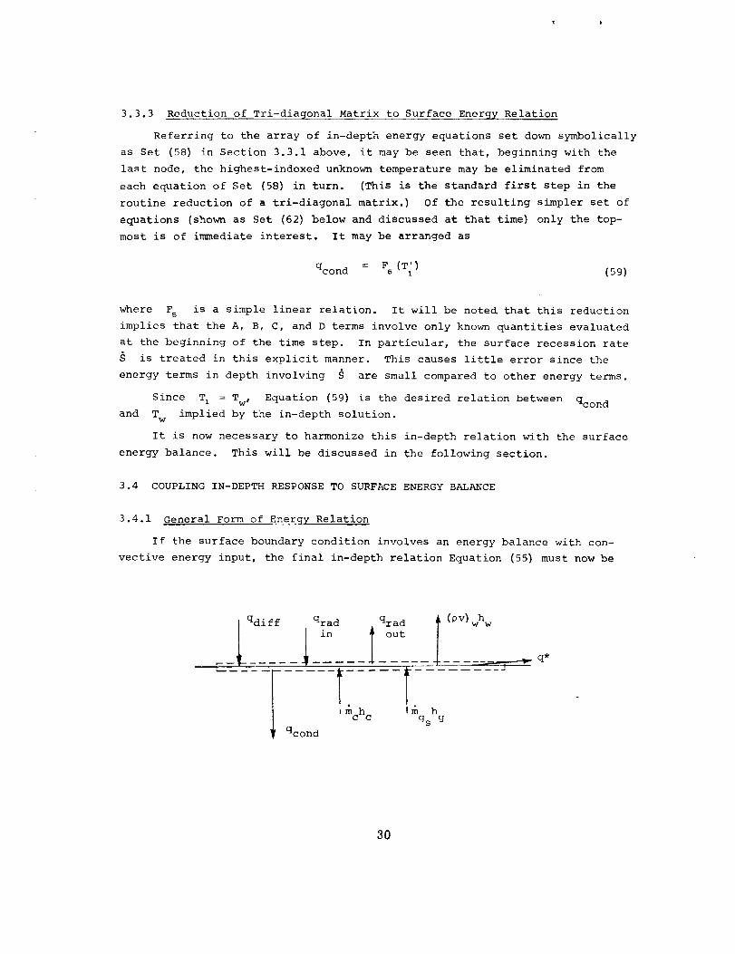
coupled to the surface energy balance illustrated in the sketch above.

surface energy balance may be written

+ qrad + -mchc + mghg -qdiff

in

The

qrad- (PV) whw- q* - qcond = 0 (60)

out

where

(_V)w = £gs + _c - r_*

We note that mg and qcond = Fs (T w)

Other dependencies of interest are

are delivered by the in-depth solution.

hg = hg (Tw) ,

= h (Tw) ,hc c

qrad = qrad(Tw )

out out

For the other terms, we have

m*' qdiff' qrad' hw' q*

in

functions of boundary layer edge enthalpy,

pressure, boundary layer aerodynamic solu-

tion, conservation of chemical element laws,

chemical equilibria and/or kinetic relations,

upstream events, mc,T w.

3.4.2 Tabular Formulation of Surface Quantities

From the standpoint of the surface energy balance solution the desired

relationship may be summarized as

m*" qdiff' qrad' hw' q* = functions of (mc,Tw)

in

where all the other aspects of the solution are subsumed in some other compu-

tational procedure, the details of which are not of immediate interest. This

other computational procedure might be based upon a simple film coefficient

model of the boundary layer, as will be described below, or it might be based

on a very detailed boundary layer solution.

31

In almost all cases, however, it proves expedient to do this solution

outside the charring material solution routine and to make the results avail-

able to the surface energy balance operation in the form of tables of qdiff'

qrad in' hw' q*' and T w as functions of mc' mgs' and another variable which

is essentially time 0 and includes all time dependent aspects such as pres-

sure.

3.4.3 Solution Procedure for the Surface Energy Balance

The energy balance solution procedure is then fairly obvious. An initial

of the char consumption rate, mc' is obtained in some manner. Withguess

supplied by the in-depth solution, the quantitiesthis mc' and with the mg

qdiff' qrad in' hw' q*' and T w are obtained by table look up in the tables

provided by the outside surface solution routine. The quantities hc, hg

and qrad out can then be formulated using the T w so obtained.

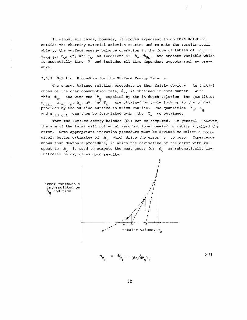
Then the surface energy balance (60) can be computed. In general, however,

the sum of the terms will not equal zero but some non-zero quantity e called the

error. Some appropriate iteration procedure must be devised to select succes-

sively better estimates of _ which drive the error e to zero. Experiencec

shows that Newton's procedure, in which the derivative of the error with re-

spect to mc is used to compute the next guess for mc as schematically il-

lustrated below, gives good results.

0

I

/

error function c /_J'/l

interpolated on

_g and time //

.1

o_I tabular values,C

m = _, - c (61)

c2 ci (dc/d_c) i

82

Since the actual c function is almost linear between tabular points (radia-

tion introduces slight curvature) this scheme converges rapidly to an answer.

Possible traps due to kinks or elbows in the e function are avoided by limit-

ing corrections on • to one tabular interval at a time.c

3.4.4 Completin_ the In-depth Solution

Once the surface energy balance has been satisfied to an acceptable level

of accuracy, the new surface temperature, T_, may be substituted in the re-

duced array of temperatures which began as Set (58). The highest-indexed

unknown temperature has been eliminated from each equation in this set in the

process of deriving Equation (59). The remaining array looks like

21

A S T'2 + B*T_ = D*3

A T's + B*T2 = D*

ANTN_I+ B_T_ = F 4 (Tres) (62)

Since T' is now known, the first equation of Set (62) yields T' directly,1

then the second equation yields T_, and so on until the new temperature set

is complete.

As a final step, new values for temperature dependent properties can be

selected for each node and the entire system is then ready for a new time step,

beginning with the decomposition event.

Alternatively, the question arises whether it might be prudent to iterate

the entire time step calculation to implicitize the quantity S (for which a

new value may be computed from the new _,c) , as well as to implicitize the

decomposition kinetics and all temperature dependent properties. Usually,

however, the quantity S exerts only a weak influence on the in-depth solu-

tion (which tends to adjust itself to damp out the effects of oscillating

values). Furthermore, all important temperature dependent property effects

have already been partly implicitized in the in-depth energy solution through

linearization. Thus the S aspect and the properties aspect do not seem to

provide much motivation for iteration.

SS

The decomposition problem is another matter. It is clear that leaving

the temperature dependence explicit in the decomposition kinetics is inviting

trouble, since for most practical problems of interest the temperature rise

is great and the decomposition rates are very sensitively dependent on tem-

perature. Indeed, practical experience shows that for violent transients

the problem solution procedure can be disrupted by instabilities due to this

explicit temperature dependence.

It is possible that a linearization of this dependence may be sufficient

to effect the solutions to most problems without the necessity for iteration.

In that case the in-depth temperature matrix is triangular instead of tri-

diagonal, but the basic solution procedure is not much modified. This device

has not yet been incorporated in the charring ablation computer program des-

cribed in Section 6 below.

Z.5 SOLUTION WITHOUT ENERGY BALANCE

The surface boundary condition need not, of course, be an energy balance.

Surface temperature and recession rate might be specified. In that case T_

is known, and the solution of Section 3.4.4 can be completed at once. The

quantity qcond is only of "cultural" interest now.

This option is especially useful for parametric studies matching inter-

nal thermocouple response predictions to the measured thermocouple responses,

using measured surface temperature and recession data, in order to "back-out"

thermal conductivity data, determining conductivity as a function of tempera-

ture and density. Frequently this procedure is required before a surface

energy balance type of calculation can be done since the required thermal

conductivity information is not generally available for many materials.

3.6 SOLUTION WITH RADIATION INPUT ONLY AND NO RECESSION

To simulate "cool-down" or "soak-out" problems, convective energy input

can be ignored and surface recession supressed. The surface temperature can

be determined with a simple version of Equation (60) in which the terms

mc' and q* are zero and for which the terms mghg andqdiff" qrad in'

(PV) wh w cancel. In this case the wall temperature is the independent variable.

34

SECTION 4

SOME NOTES ON PROPERTY VALUES

4.1 INTRODUCTION

Some remarks on the various physical property values required for the

in-depth solution may help to clarify certain aspects of both the analysis

of Section 3 above and the associated computer program. Features which are

especially important or somewhat unusual (when compared to most other compu-

tation schemes) will be stressed.

4.2 DENSITIES

Section 3.2.3.3 above describes how the decomposition kinetic relations

are written for three independently pyrolyzing components requiring Poi,

the initial (virgin) density for each component i, and Pri, the final

(char) density for each component. Thus the user must supply po i and pr i

for each component, and the resin volume fraction F. The program itself

computes the overall virgin and char densities from this data.

The user frequently starts with measured values of virgin and char den-

sities and partitions these densities up among the decomposing constituents

according to the decomposition kinetic data he is trying to match. The next

section gives some discussion of this point.

4.3 KINETIC DATA

Equation (4b) of Section 3.2.3.3 indicates that in addition to the po i

and Dr i data, the kinetic constants k i, m i and ei/R are required for

each constituent of the decomposing material. The required data, much of

which may be located in the literature, are obtained from thermogravimetric

(TGA) experiments. The observed decomposition kinetics may be modelled with

one, two, or three kinetic regimes as required. Experience shows that more

than three regimes are not required for materials of current interest.

Indeed, the great majority of materials is well described by only a single

kinetic relation.

As noted in Section 4.2 above, the selection of the decomposing consti-

tuents influences the partition of the densities among the component densi-

ties and0o i Pr i

It will be noted that the decomposing constituents are selected to match

TGA data and have no explicit connection to the identification of actual

molecule types. Of course, it frequently happens that constituents clearly

35

identifiable on TGA traces do represent particular molecules or groups of

similar molecules, but this is a secondary matter of no significance to the

in-depth solution.

4.4 SPECIFIC HEATS

The transient in-depth solution naturally requires data on the specific

heats of the virgin material and the char. These are supplied to the program

as tabular functions of temperature.

For partially degraded material with Pc < p < Pp' the analysis of Sec-

tion 3.2.3.4 above has introduced the model that the specific heat is a par-

ticular kind of mass mean specific heat. In this model, partially degraded

material is thought of as a mixture of pure char and pure virgin material.

The specific heat (and hence the enthalpy) of partially pyrolyzed material

is thus a mass weighted average of the virgin and char specific heats.

This model is convenient and plausible. Furthermore, the specific heats

of virgin and char material usually differ only slightly, so that the choice

of a mixture model is not very important.

4.5 HEAT OF FORMATION

Enthalpies for char and virgin material are computed as integrals of the

specific heat function from the datum temperature to the temperature of inter-

est, plus a heat of formation. Equations (22) and (23) above indicate this

calculation. Hence, the user of the computer program must supply heat of for-

mation data. For mcst materials such data may be found in various tabulations,

or may be derived from heat of combustion or heat of pyrolysis data. In the

case of materials for which no measured data are available, the required heats

of formation may usually be obtained by theoretical methods or from rules of

thumb regarding the amount of energy associated with each type of chemical

bond. For most materials the heats of formation of char and virgin plastic

have only a minor effect on any ablation results, and hence, great accuracy is

not required.

The pyrolysis gas heat of formation is much more significant and will be

discussed in Section 4.7.

4.6 HEAT OF PYROLYSIS

Inspection of the energy Equation (39) reveals that the "heat of pyrolysis"

or energy effect associated with the degradation of virgin material to char

is given by (h - hg),Btu per pound of pyrolysis gas formed. The computer

36

program automatically calculates this temperature dependent quantity as needed,

employing the input specific heat functions and heats of formation.

4.7 PYROLYSIS GAS ENTHALPY

The in-depth energy Equations (38) and (39) indicate that it is most con-

venient to have the pyrolysis gas thermal properties as a simple tabulation

of enthalpy versus temperature. If it can be assumed that the pyrolysis gases

are in chemical equilibrium as they pass through the char, it is a simple matter

to run a series of equilibrium chemistry solutions with any convenient compu-

tation scheme to obtain the necessary enthalpy table, provided that the ele-

mental make-up of the gas is known. The required elemental data can be ob-

tained from virgin and char density and elemental analysis measurements.

Unfortunately, such equilibrium calculations often indicate that solid

carbon particles should precipitate out of the pyrolysis gas. Allowing these

particles to collect on the char structure complicates the analysis enormously

(see the sixth report of the present series). Thus the analyst is tempted to

either

(i) Allow the solid carbon to form, but require it to travel out of

the char with the gases

(2) Suppress carbon formation in the enthalpy calculation, thus intro-

ducing a kinetic consideration.

Both of these techniques are often tried in practice.

To do an accurate calculation of the pyrolysis gas enthalpy accounting

for all possible kinetically controlled reactions would be very difficult

and would require information about the initial molecular configurations in

the pyrolysis gas, information not usually available. It is important to

recognize, however, that the in-depth solution only requires an enthalpy-

temperature function, so that any physical model for which data are available

can be accommodated without any changes. In this sense the treatment of the

pyrolysis gas kinetics is quite general, excluding only carbon deposition

("coking") and char erosion. Changes of gas enthalpy with pressure are sec-

ondary and are ignored.

It is unfortunate that energy absorption by the pyrolysis gases as they

pass through the char is very important for most materials of interest.

Hence, it is important to choose a physical model which is accurate in obtain-

ing the gas enthalpy curve.

37

4.8 THERMAL CONDUCTIVITY

Thermal conductivity, as a function of temperature, is required for the

virgin material and the char. Conceptually, this presents no difficulties

although in practice good data are very hard to obtain. (Many of the applica-

tions of the computer program are for backing-out conductivity data from

measured thermocouple responses taken from instrumented test samples.)

The treatment of conductivity for partially degraded material is a con-

troversial, interesting, obscure, and very important topic. In the past it

it was deemed sufficient to follow the model used for specific heat and to

use a linear interpolation on virgin material mass fraction:

k = Xkp + (i - x) k c

where the partially degraded material is regarded as a mixture of virgin mate-

rial and pure char. The quantity x is the pounds of virgin per pound of

partially degraded substance. It equals unity for virgin plastic and zero

for pure char, and at intermediate densities can be shown to be

C °c)---- 1 --

X Pp- _C _--

Recent experiments have shown, however, that while this model may be a

good one for specific heat it can sometimes be a very poor one for thermal

conductivity. Many materials display, shortly after decomposition begins,

a conductivity appreciably lower than either the virgin conductivity or the

char conductivity, a circumstance which cannot be predicted by the model

described above. Therefore, a recent modification to the computer program*

has introduced a more general expression

k = fl (X) kp + f (x) k c

where fl and f2 can be input as general tabular functions of x. With this

device, formerly inexplicable in-depth thermocouple response could be "pre-

dicted" quite accurately. It appears that the surface temperature history is

*This work is reported in Rindal, R. A., Clark, K. J., and Moyer, C. B.:

Experimental and Theoretical Analysis of Ablative M=terial Response in a

Liquid Propellant Rocket Engine, Fourth Quarterly Progress Report, NASA

Lewis Research Center, Cleveland, Ohio, Contract No. NAS3-7945, 1966.

38

little affected by the new model for mixture conductivity, but the temperature

profile through the narrow pyrolysis zone is drastically altered for those

materials in which the conductivity depression is marked, in particular the

rapid decomposers such as nylon phenolic.

4.9 SURFACE EMISSIVITY e

The role and importance of this temperature dependent quantity need no

elaboration. The chief difficulty is to obtain good data. If partially de-

graded material is at the surface, the emissivity of virgin material and char

may be averaged in the same manner as the specific heat.

4.10 HEAT OF ABLATION, HEAT OF COMBUSTION

The reader will note that no such quantity as heat of ablation or heat

of combustion is required as input information for the surface energy balance

options of the analysis. It will be recalled that in these options the in-

depth solution is coupled to a general chemistry solution. Heats of ablation

and beats of combustion are empirical devices designed to circumvent the chem-

istry solution. These approaches have their advantages, but they are diffi-

cult to generalize. The only reliable general procedure involves a complete

surface chemistry solution. With such a solution in hand it is possible to

calculate the heat of ablation or heat of combustion as a matter of interest

and for correlating purposes.

4.11 SURFACE SPECIES

The identity of the chemical species existing at the ablating surface

is usually not evident a priori for complex materials. This information is

not required as input, however. It is a consequence of the chemistry solution.

4.12 CONCLUSION

The analysis has been formulated to require the input of fundamental

physical information in such a way as to preclude any inconsistencies in

energy terms (such as enthalpies) and in mass terms. Within these restric-

tions, only input of directly measureable data is required. The three items

which are probably most important in their influence on computed results,

the gas enthalpy, the thermal conductivity, and the surface emissivity, are

unfortunately the items most difficult to obtain good data for, but this,

of course, is an inherent feature of the problem, not a peculiarity of the

analysis presented.

39

SECTION 5

NOTES ON FILM COEFFICIENT MODEL OF THE BOUNDARY LAYER

WITH HEAT TRANSFER, MASS TRANSFER, AND CHEMICAL REACTION

5.1 INTRODUCTION

Section 3.4 above described in general terms how the in-depth energy solu-

tion can be coupled to the heated surface energy balance boundary condition.

This coupling is made, through the energy balance, to some computational scheme

which accounts for the basic transport physics (momentum, energy, chemical

species) and the basic conservation laws for the boundary layer.

The boundary layer integral matrix procedure developed under the present

contract and presented in coded form as the BLIMP program consitutes a very

accurate and complete procedure for generating boundary layer transport solu-

tions suitable for this coupling. As might be expected, however, this complex

routine consumes much valuable computer time for each solution. Hence, economic

considerations encourage the use of some simpler boundary layer procedure when-

every possible.

For this purpose the basic in-depth charring material solution procedure

has been coupled to a film coefficient boundary layer model which offers speedy

and economical approximate solutions which still retain all of the essential

chemical features of ablation events. Thus the in-depth program exists in

coupled form in two distinct versions, one coupled to the BLIMP program, and

one coupled to a film coefficient model. Section 3.4 above describes the cou-

pling in general terms applicable to both coupled versions. For details on

the BLIMP program add the associated integral analysis the reader may refer

to the summary report of the present series (in preparation - see Foreword)

and to Referenze 35. Unfortunately, a corresponding detailed presentation of

the fundamentals of the film coefficient model used for the other coupled ver-

sion has not previously been presented. Therefore the present section offers

a few remarks on the film coefficient model as supplementary information.

Since the chief purpose of the present report is to describe the in-depth solu-

tion procedure, the following remarks on the film coefficient surface model

will be in outline form, with arguments and developments omitted.

5.2 GENERAL POSITION, IMPORTANCE, AND HISTORY OF FILM COEFFICIENT MODELS

APPLIED TO MASS TRANSFER WITH CHEMICAL REACTIONS

5.2.1 General Remarks

Probably the great majority of boundary layer heat and mass transfer

solutions with chemical reactions have been built on either

40

(i) An empirical approach for any given problem, or

(2) A complete, accurate solution applied to specific, restricted

chemical systems.

Each of these alternatives can be well defended for particular problems. In

the development of large and costly computer programs, however, it is important

to build in as much generality as possible. It has been known for a long time

that film coefficient boundary layer models, originally developed for heat

transfer calculations, can provide much generality by an extension to include

mass transfer effects. The film coefficient approach provides the necessary

transport information, and some appropriate chemical solution routine can pro-

vide the necessary chemistry solution.

The fundamental analysis involved in using such a film coefficient scheme

involves two key parts:

(i) Derive the film coefficient mass transport relations, and

(2) Derive the film coefficient energy transport relation

The actual use of the formulation requires another step, that of calculating

the film coefficients PeUeCH and PeUeCM . This final aspect is not simple,

especially for high rates of mass transfer (blowing) from the surface, and

indeed for strongly non-similar boundary layers probably cannot be carried out

in a useful way. Nevertheless this task can be carried out for a great many

problems of importance.

The first two tasks cannot be carried out without specific consideration

of the calculation of the film coefficients unless rather loose, heuristic

arguments are accepted. The number of cases in which Steps (i) and (2) can

be carried out with precision is rather small.

In one particular case, however, Steps (i) and (2) can be carried out:

if Le = 1 and all mass diffusion coefficients are equal, then for a great

many problems it is possible to calculate PeUeCH , demonstrate that C M = C H,

and carry out Steps (i) and (2) without difficulty, regardless of the complexity

of the chemical events involved. References 36 and 37 provide many examples

of combined heat and mass transfer for this case, covering a very wide range

of application areas. This simple model is included as part of the coupled

computational procedures, but since it appears as a special case of a more

general formulation to be described below, any further discussion will be post-

poned.

Although the Le = 1 and CM/C H = 1 case proyides very powerful sim-

plicities in analysis, it is quite frequently not an accurate representation

41

of the physical situation in rocket nozzle and reentry problems. The very

wide range of molecular weights of the chemical species involved makes the

equal diffusion coefficient assumption inaccurate.

Therefore, there is a strong incentive to extend the film coefficient

formulation to cases in which, as a first improvement, C M / CH, and as a

further improvement, the mass diffusion coefficients are not equal. In the

sections below we shall consider these improvements in turn.

5.2.2 History of Film Coefficient Model for C M / C H

It can be shown, for the case in which Le _ 1 but all the mass diffusion

coefficients are equal that it is generally possible and useful to write the

diffusive flux of a chemical element away from the wall to the boundary layer

as

_k = PeUeCM(_ - Kk )w w e

(63)

Extended discussions of this relation may be found in References 24, 26, 37,

and 38.

The corresponding energy transfer relation is not so easily established,

unfortunately. Exact arguments can be carried through only for the case

C M = CH; for the present case some limiting or perturbation type arguments

can be carried through for special problems. For example, the case of no net

mass transfer and a frozen boundary layer is considered in a heuristic way

in References 37 and 39. Spalding gives a summary of the state-of-the-art

for this special problem in Reference 40, along with an extensive bibliography.

Lees discusses this case in Reference 41, along with a number of other cases

to be mentioned later, as do Fay and Riddell for the specific case of air in

Reference 42. For "almost frozen" boundary layers (still with no net mass

addition) Spalding gives brief discussions of the recommended film coefficient

energy equation in References 37 and 40. For very reactive boundary layers

with no net mass addition, discussions are given by Lees in Reference 41,

quoting only Fay and Riddell's results for air in Reference 42.

For the more important case of net mass addition to the boundary layer

with chemical reactions, the discussions presented in the literature for the

case C M J C H appear to be limited to Lees in Reference 41 for the frozen

boundary layer and to References (26) and (38). The Lees analysis considers

the governing boundary layer differential equations and derives, for the frozen

boundary layer case, an expression for the rate of energy transfer to the wall

42

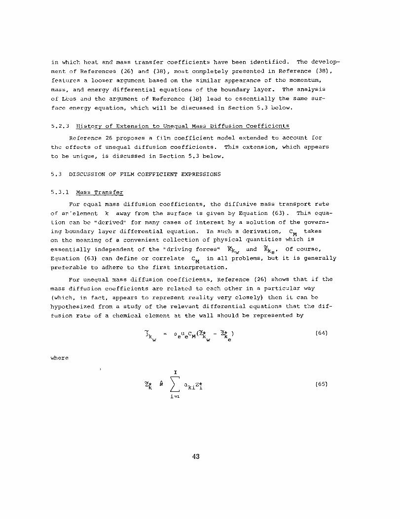
in which heat and mass transfer coefficients have been identified. The develop-

ment of References (26) and (38), most completely presented in Reference (38),

features a looser argument based on the similar appearance of the momentum,

mass, and energy differential equations of the boundary layer. The analysis

of L_es and the argument of Reference (38) lead to essentially the same sur-

face energy equation, which will be discussed in Section 5.3 below.

5.2.3 History of Extension to Unequal Mass Diffusion Coefficients

Reference 26 proposes a film coefficient model extended to account for

the effects of unequal diffusion coefficients. This extension, which appears

to be unique, is discussed in Section 5.3 below.

5.3 DISCUSSION OF FILM COEFFICIENT EXPRESSIONS

5.3.1 Mass Transfer

For equal mass diffusion coefficients, the diffusive mass transport rate

of an'element k away from the surface is given by Equation (63). This equa-

tion can be "derived" for many cases of interest by a solution of the govern-

ing boundary layer differential equation. In such a derivation, C M takes

on the meaning of a convenient collection of physical quantities which is

essentially independent of the "driving forces" _kw and Kke. Of course,

Equation (63) can define or correlate C M in all problems, but it is generally

preferable to adhere to the first interpretation.

For unequal mass diffusion coefficients, Reference (26) shows that if the

mass diffusion coefficients are related to each other in a particular way

(which, in fact, appears to represent reality very closely) then it can be

hypothesized from a study of the relevant differential equations that the dif-

fusion rate of a chemical element at the wall should be represented by

_k = 0eUeCM (_ - _ )w w e

(64)

where

I

i=l

(65)

43

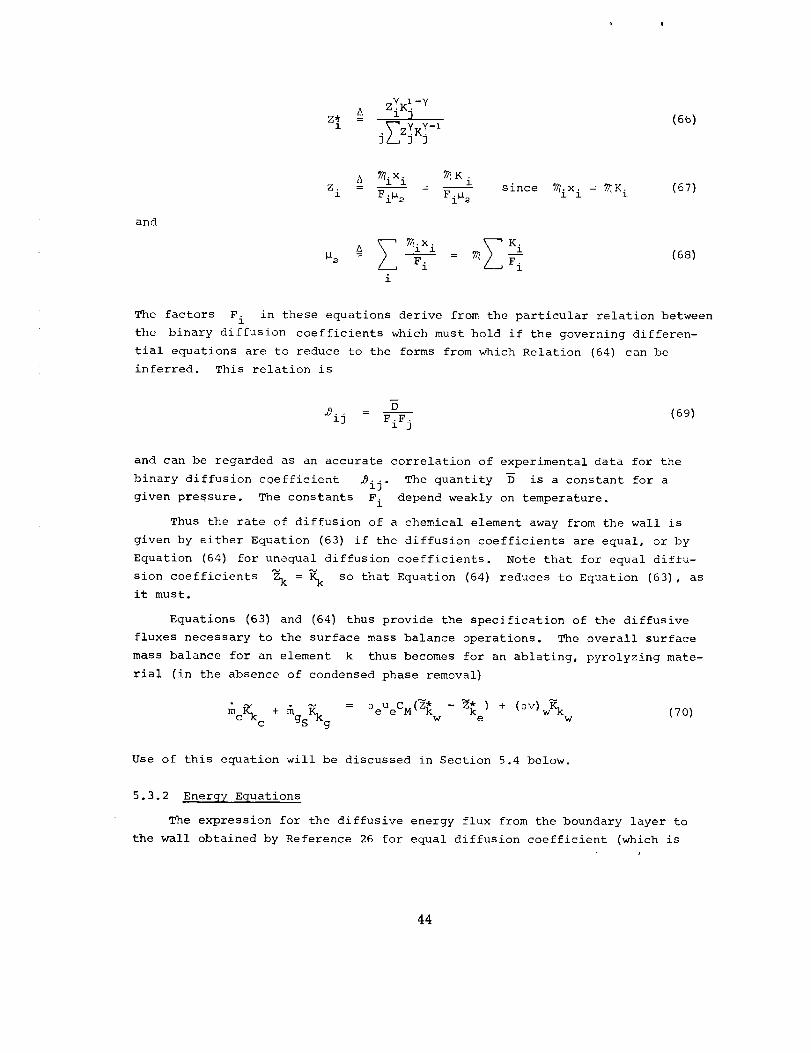
zYx_,-YZ*. = 1 ] (6b)

.T'zV, 1<Y,-_3/.3 J

and

A _ixi _ K i

• = - since _ixi = _K i (67)Zl FiU 2 FiU e

P2 = Fi - _ F_i (68)

i

The factors F i in these equations derive from the particular relation between

the binary diffusion coefficients which must hold if the governing differen-

tial equations are to reduce to the forms from which Relation (64) can be

inferred. This relation is

m

D

dgiJ - F.F. (69)J

i 3

and can be regarded as an accurate correlation of experimental data for the

binary diffusion coefficient 29ij. The quantity _ is a constant for a

given pressure. The constants F i depend weakly on temperature.

Thus the rate of diffusion of a chemical element away from the wall is

given by either Equation (63) if the diffusion coefficients are equal, or by

Equation (64) for unequal diffusion coefficients. Note that for equal diffu-

sion coefficients _ = % so that Equation (64) reduces to Equation (63), as

it must.

Equations (63) and (64) thus provide the specification of the diffusive

fluxes necessary to the surface mass balance operations. The overall surface

mass balance for an element k thus becomes for an ablating, pyrolyzing mate-

rial (in the absence of condensed phase removal)

me% c + mgsKkg 0eUeCM(Z{w _{e ) + (Pv) jKkw (70)

Use of this equation will be discussed in Section 5.4 below.

5.3.2 Energy Equations

The expression for the diffusive energy flux from the boundary layer to

the wall obtained by Reference 26 for equal diffusion coefficient (which is

i

44

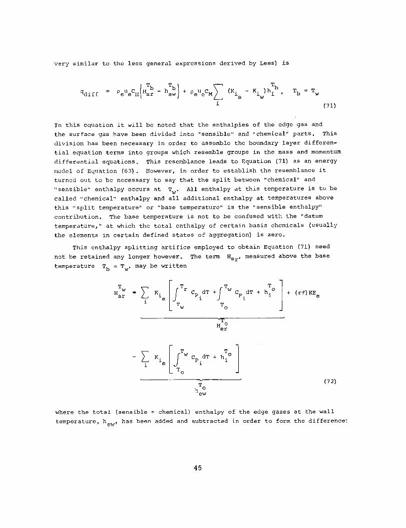
very similar to the less general expressions derived by Lees) is

Tb ) _ Tbqdiff P eUeCH Hsr h:bw + P eUeCM (Ki e - Ki w) == - hi ' Tb Tw

(71)

In this equation it will be noted that the enthalpies of the edge gas and

the surface gas have been divided into "sensible" and "chemical" parts. This

division has been necessary in order to assemble the boundary layer differen-

tial equation terms into groups which resemble groups in the mass and momentum

differential equations. This resemblance leads to Equation (71) as an energy

model of Equation (63). However, in order to establish the resemblance it

turned out to be necessary to say that the split between "chemical" and

"sensible" enthalpy occurs at T w. All enthalpy at this temperature is to be

called "chemical" enthalpy and all additional enthalpy at temperatures above

this "split temperature" or "base temperature" is the "sensible enthalpy"

contribution. The base temperature is not to be confused with the "datum

temperature," at which the total enthalpy of certain basis chemicals (usually

the elements in certain defined states of aggregation) is zero.

This enthalpy splitting artifice employed to obtain Equation (71) need

not be retained any longer however.

temperature T b = Tw, may be written

The term Hsr , measured above the base

ljTridTjTwT]H w = Ki Cp + Cp dT + h. °sr 1

i e l

T w T O

_mH oer

+ (rf) KEe

- K i Cp dT + i

i e i

T O

v (72)T

h oew

where the total (sensible + chemical) enthalpy of the edge gases at the wall

temperature, hew _ has been added and subtracted in order to form the difference:

45

T

H w (Rr - h)sr = edge gas (73)

T

Recalling that h w = 0, we may writeSW

HW-h w = Hr-hsr sw w edge gas (74)

where the total enthalpies in the above relation may be evaluated above any

datum temperature. Note that the enthalpy of the edge gas at wall tempera-

ture is for the chemical composition frozen at the boundary layer edge condi-

tions, no___tthe equilibrium enthalpy of edge gas at the wall temperature.

Hence the diffusive flux qdiff becomes

T

qdiff = PeUeCH(IIr - hw)edge + PeUeCM _. (Ki e - Ki )hiW (75)W

gas i

The T w in the final term is now the last remnant of the splitting operation,

but h_ w merely means the enthalpy of molecular species i at the wall tem-

perature. The quantity (Hr - hw) edge gas does not depend on the choice of

the base state since each enthalpy is for the same physical material, namely

frozen edge gas.

Now the overall surface energy balance may be written as

T 1)h w + B'h + B'h - B'h- - Ki l c c g g w?eUeCH(Hr hw)£dge + PeUeCM (Kie w

gas

+ ewqra d - F_ET_ - qcond = 0 (76)

Only one final detail deserves attention. Equations (75) and (76) have

been derived in Reference 38 with rather loose arguments. Any checks on the

correctness and applicability of these equations are of importance. One key

check requires the results computed from Equation (76) to be independent of

the enthalpy datum state. A lengthy argument can be constructed to show that

this is the case. (Equation (75) alone does depend on the datum state, ofT w

course, through the h. term.)i

As a final point it may be observed that the derivation of Equations (75)

and (76) given in Reference 26 does not include any restrictions about the

46

location of the chemical reactions. It cannot be firmly concluded, however,

that Equation (75) holds for a strongly reacting boundary layer (except, of

course, in cases where Equation (75) is used to define C M or CH). Indeed,

the separation between the frozen term for heat transfer and the enthalpy

term" for mass transfer suggests that Equation (75) applies only to a frozen

boundary layer, reactive wall case. Furthermore, frozen boundary layer analy-

ses lead to equations equivalent to Equation (75) in References 40 and 41.

Lastly, physical arguments can be constructed to suggest that for highly re-

active boundary layers it should be impossible to write general equations

of the form of Equation (75). The discussion of pages 263-275 of Reference

37 is of interest in this regard.

It may be expected that Equations (75) and (76) may apply with good

accuracy to frozen and nearly frozen boundary layer problems, but are probably

less accurate for reactive boundary layers. An indication of the accuracy

of equations such as (75) for highly reactive boundary layers may be obtained

by referring to the numerical boundary layer solutions of Fay and Riddell

(Reference 42). Fay and Riddell's results differed only slightly whether the

boundary layer was treated as frozen with a catalytic wall or if equilibrium

was assumed throughout the boundary layer. Even though their solutions are

limited to air stagnation flow it is believed reasonable to generalize their

conclusion* to include gases other than air and for body locations other than

the stagnation point. If this generalization is accepted, Equation (75) may

be employed for equilibrium, as well as frozen boundary layers, with little

loss in accuracy.

Reference 26 extends Equations (75) and (76) to the case of unequal mass

diffusion coefficients by analogy arguments. The resulting equations resemble

Equation (64). The diffusional energy flux to the wall becomes

qdiff = PeUeCH(Hr - hw) edge + PeUeCM _ (Z_ - Z_l )h_wl (77)e w

gas i

and the overall energy balance becomes

*"... the heat transfer is almost unaffected by a nonequilibrium state of

the boundary layer provided the wall is catalytic and the Lewis Number near

unity."

47

PeUeCH(Hr - hw) edge +OeUe C (Z* - Z_ )h i + c c g g w

gas . e w

+ _wqrad - FoCT_w - qcond = 0 (78)

Equations (77) and (78) are somewhat less well founded than the corres-

ponding Equations (75) and (76), but the equations do have plausibility.

Furthermore, the equations reduce to Equations (75) and (76) for equal dif-

fusion coefficients, as they should, and Equation (78) can be shown to be

independent of the enthalpy datum state and thus fulfills a basic physical

requirement.

5.4 USE OF FILM COEFFICIENT EQUATIONS TO CALCULATE SURFACE

ENERGY BALANCE

5.4.1 Basic Aspects

The film coefficient model has provided simple expressions for the dif-

fusive transport rates of mass and energy through the boundary layer to the

wall. It is now necessary to indicate how these relations may be expeditiously

used in computing the surface energy balance. Section 3.4.2 above describes

how it is useful before doing the surface energy balance, to have the diffu-

sive flux terms and hw, q*, and T w as functions of m and m beforec gs

forming the energy balance. For this purpose, the film coefficient mass

transport relations may be coupled to some convenient chemistry routine which

solves the coupled mass balance + chemistry problem. Equations (75) and (78)

suggest that mc and mgs can be normalized on PeUeCM to increase the gen-!

erality of this procedure. B c and B' can then be regarded as independentg

variables in the construction of a table of values of Tw, _ Z_eh_W and

_Z* h Tw 'i w i for given pressure, edge composition, char composition, and gas

composition. (The term q* may be lumped with this last term if desired.)

The resulting table meets all the requirements outlined in Section 3.4.2

and can be used for an iterative determination of that B' which satisfiesc

the surface energy balance, given B_ from the in-depth solution.

The Aerotherm Equilibrium Surface Thermochemistry Program (EST) is a

coupled mass balance - equilibrium chemistry routine which generates such

tables for chemical equilibrium conditions. Reference 43 describes this

program. A somewhat newer version with improved computational techniques is

denoted the Aerotherm Chemical Equilibrium Program (ACE) and is described

48

in Reference 44. This program allows certain reactions to be kinetically con-

trolled and hence has more generality.

5.4.2 Input and Correction of Heat Transfer Coefficient

To employ the film coefficient formulation just described, the program

user must provide the program with values of the heat transfer coefficient

PeUeCM as functions of time. Two practical problems must be settled in this

respect:

(i) How is C M related to CH?

(2) Can both C M and C H be specified as functions of edge conditions

(i.e., of time) independent of the subsequent problem solution

(i.e., mass transfer rates and body shape)?

In answer to the first question it may be stated that within the present

formulation it is adequate to take the ratio CM/C H as a constant. The value

of this constant is a measure of the ratio of the mean mass transfer aspects

of the boundary layer to the mean heat transfer aspects. For equal mass dif-

fusion coefficients, a vast amount of experimental data (as summarized, for

example, in Reference (37)) suggest the correlation CM/C H = Le ¥. It may be

hypothesized that for unequal mass diffusion coefficients the same procedure

may be employed with the Lewis Number, Le, defined by the procedure set forth

in Reference 26 involving D. Thus, the input to the program consists of a

time table of values for PeUeCM and the constant factor CM/C H.

The answer to question (2), changes of C H with body shape are occasionally

of interest and may easily be accounted for. A more important problem concerns

the dependence of C H on the actual rate of mass transfer. This problem has

been ignored up to now, the implication being that C H is determined by the

boundary layer edge aerodynamics alone. This is known to be incorrect. The

value of C H depends fairly strongly on m. If we denote the C H with m = 0

as CH0, this dependence is shown by both data and analysis to be accurately

represented by

(79)

where

2km= (80)

PeUeCt{o

49

Equation (79) accurately correlates a large amount of laminar data if _ is

chosen as 0.5. For turbulent flow a _ of 0.4 appears to be slightly better.

The computer program provides for _ as an input parameter and then automati-

cally computes the "blowing reduction."

5.5 CONCLUSIONS

A film coefficient model for boundary layer heat and mass transfer with

chemical reactions can be developed for the governing differential equations

of the boundary layer. Of the resulting film coefficient expressions, those

for mass transport can be coupled to any convenient chemistry routine to pro-

vide boundary conditions for an in-depth response calculation. The boundary

information and the in-depth calculation are coupled through the film coef-

ficient surface energy balance, providing a complete link between the boundary

layer and the sub-surface material.

The film coefficient model of the boundary layer provides a powerful,

economical, and quite general alternative to empirical procedures and to

elaborate "exact" procedures. The model can be proved to be accurate for a

wide range of problems, and appears to apply with good accuracy for an even

wider range of problems for which good accuracy proofs cannot be constructed.

SECTION 6

PRESSURE DROP

The pressure drop across the char layer resulting from pyrolysis gas

flow is of interest because it may give rise to excessive char stress levels.

Knowledge of the pressure distribution through the char is necessary for evalu-

ating char layer stress levels. An empirical relation for evaluating the

pressure distribution through the char layer is rationalized and presented

first, in Section 6.1 and is followed, in Section 6.2 by the finite difference

formulation.

6.1 PRESSURE DROP CORRELATION EQUATION

In order to obtain an expression relating local pressure in the char

layer to other pertinent variables it is useful to examine experimental data

taken for a range of variation of the pertinent parameters of interest, and

to deduce the most significant effects by generalizing this data. The data

presented by Green in Reference 45 is employed for this purpose. Green

presents a compilation of data for flow of various gases through a wide variety

of porous media for a large range of flow conditions. In order to relate

5O

pressure gradients to viscous and inertial forces he employs the correlation

equation first proposed by Reynolds:

d__PP = _v + _pv _ (81)dy

where the first term represents viscous forces and the second, momentum forces.

The quantities a and 8 are empirical coefficients, _ is the gas viscosity,

and p is the gas density. The velocity (v) in Equation (81) is a "super-

ficial velocity" defined on the basis of the gas flow rate per unit projected

area in a plane normal to the velocity vector.

v _ --q (82)pA

Referring to the above equations, the ratio of inertial to viscous forces may

be written as:

Inertial Force = Bmg

Viscous Force _A

The compilation of data presented by Green includes tabulations of the empir-

ical coefficients _ and 8 for a wide variety of porous media including

packed beds of irregular and spherical particles ranging in nominal size from

0.08 inch to 0.1875 inch and for close packed wire screens ranging from 60

to 5 mesh. The nominal range of porosities included varies fr_n 0.3 to 0.8.

The experimentally derived coefficients _ and 8 are shown in Figure 3

along with a straight line fit to the data.

= 0.794 x 104

where a has units of ft -_ and 8 has units of ft -I . The correlation is

not excellent, but appears appropriate for order-of-magnitude considerations.

Substituting this relation into the equation obtains

Inertial Force

Viscous Force= 1.26 x 10 -4 --q

_A

For the temperature range of interest (2000°R - 5000°R) the gas viscosity will

range from about 0.3 x 10 -4 to 0.5 x 10 -4 Ib/ft-sec. Considering a gas vis-

cosity of 0.4 x 10 -4 ib/ft-sec, the ratio of inertial to viscous forces may

be written:

51

Inertial Force = 3.15 --qViscous Force A

where mg/A has the units of ib/ft_-sec. It may therefore be concluded that

for pyrolysis gas flow rates of 0.01 ib/ft_-sec and less, the inertial terms

may be ignored in which case Equation (81) reduces to Darcy's Law.

dP

d-_ = _v

where -i is the permeability. It is believed appropriate, however, that

the more complete correlation Equation (81) be employed for pressure drop

calculations in the char layer of ablating materials since it is valid for

a wider range of conditions of practical interest.

6.2 FINITE DIFFERENCE FORMULATION

It is desired to cast the pressure drop correlation Equation (81) into a

form including only variables which are readily available from the computation

scheme for solving the mass and energy conservation equations (Section 3.2.4).

The velocity of the gas passing through the porous char is related to

the gas flow rate per unit area by Equation (82). Introducing the gas state

equation (P = 0gRT/_g) into Equation (82) yields:

----q-- RT (83)

v = P_gA

It is convenient to define a viscosity law for the pyrolysis gas

= _o (84)

Substituting Equations (83) and (84) in (81) yields the following rela-

tion for a linear pressure drop across a node (n, see Figure 2).

I [CTIn:dY n _o + 8 A-_(85)

where the coefficients _, B, and the gas molecular weight, _g are input

as functions of temperature and mg n represents the pyrolysis gas flow rate

entering the node n. Equation (85) is solved for n = 1,2,3 ..., down to

the first node in the virgin material where mgn = 0. The pressure at the

52

top of node 1 is taken equal to the prescribed boundary layer edge pressure

(PI = Pe ) " The pressure at the top of any other node is related to the pres-

sure drop across and pressure at the top of the node above it.

= p + --%d._ 6 (86)

Pn n-i ay] n-i n-i

or

n-i

Pn Pe EId )i°i 87i=l

The computation is performed in an explicit manner, that is, after obtaining

solution of the energy and mass conservation equations, a single pass through

the nodal network from heated surface (n = i) to the virgin material yields

the pressure distribution entirely in terms of conditions existing at the end

of the-previous time step.

SECTION 7

SOME OPERATIONAL DETAILS OF THE AEROTHERM

CHARRING MATERIAL ABLATION PROGRAM, VERSION 2

7.1 INTRODUCTION

While it is not the purpose of the present document to offer a detailed

description of the charring material computer program which is based upon

the analysis presented in Section 3 above, it does seem useful to include

a few words of program description at this time. Complete descriptions,

user's manual, and flow charts are given in References 46, 47, and 48.

7.2 PROGRAM DESCRIPTION

7.2.1 General Remarks

The Charring Material Ablation (CMA) program is a coded procedure for

calculating the in-depth thermal response of a charring, ablating material.

The solution is obtained through difference equations discussed in Section 3

above. This section presents a brief over-view of the program operation

and output.

53

7.2.2 P_rogram Objectives

The program produces in-depth temperature and density histories, plus

surface recession rate as a function of time. In addition to this basic out-

put, the program outputs a number of integrated energy terms and various mate-

rial property data of interest. Section 7.2.5 below gives a more detailed

description of the program output.

7.2.3 Program Capabilities

_le Charring Material Ablation Program is an implicit, finite-difference

computational procedure for computing the one-dimensional transient transport

of thermal energy in a three-dimensional isotropic material which can ablate

from a front surface and which can decompose in depth. Decomposition reac-

tions are based on a three-component model. The program permits up to eight

different backup materials of arbitrary thickness. The back wall of the com-

posite material may transfer energy by convection and radiation.

In one program configuration, the ablating surface boundary condition

may take one of three forms:

Option 1 - Film coefficient model convection-radiation heating with

coupled mass transfer, including the effects of unequal

heat and mass transfer coefficients (non-unity Lewis

number) and unequal mass diffusion coefficients. Surface

thermochemistry computations presume chemical equilibrium

at the surface.

Option 2 - Specified surface temperature and surface recession rate

Option 3 - Specified radiation view factor and incident radiation

flux, as functions of time, for a stationary surface.

Any combination of the first three options may be used for a single

computation. Option 3 is appropriate to cooldown after termination of con-

vective heat input and is often useful in conjunction with Option 1 and 2.

In another configuration, the program may be coupled to the Boundary

Layer Integral Matrix Procedure. In this arrangement, the total assembly

is designated the CABLE program and is described in other reports of this

series (see Foreword).

The program permits the specification of a number of geometries:

(i) Plane

(2) Cylindrical or annular, with heated surface either inner

or outer

54

(3) Spherical or spherical shell, with heated surface either inner

or outer

(4) General "thermal stream tube" geometry, area varying as depth

to any power

(5) General "thermal stream tube" geometry, area varying arbitrarily

with depth.

The rear surface of the last node may be specified as insulated, or may

experience convective and radiative heat transfer to a "reservoir" at a spe-

cified reservoir temperature if a rear surface convection coefficient and an

emissivity are input.

Material properties such as thermal conductivity, specific heat, and

emissivity are input as functions of temperature for virgin plastic and char.

For partially decomposed material, the program performs an appropriate averag-

ing to determine effective material properties.

7.2.4 Solution Procedure

The basic solution procedure is by a finite difference approach. For

each time step, the decomposition relations are solved and then the in-depth

energy fluxes constructed in general terms. These are then harmonized with a

surface energy balance (if a surface energy balance option is being used) and

the in-depth temperatures determined. New material property values are set

up and the solution is ready for the next time increment.

7.2.5 Output Information

The CMA program outputs instantaneous mass ablation rates and blowing

parameters for char and pyrolysis gas, total integrated mass ablation of char

and pyrolysis gas, total recession and recession rates of surface, of the char

line, and of the pyrolysis line. It also outputs the surface energy flux

terms, namely, the energy convected in, energy radiated in, energy reradiated

out, chemical generation, and conduction away (qcond) . Further, it describes

how the input energy of qcond is "accommodated" or "partitioned" in the

solid material. Part of the energy is consumed in decomposing the plastic,

part is consumed in sensible enthalpy changes of the solid, and part is

"picked-up" by the pyrolysis gases as they pass through the char.

Finally, nodal temperature, density and enthalpy are given for every de-

sired output time, as well as a description of the current material state for

each node.

55

Thermocouple and isotherm output can also be called for. Figure 4 shows

a representative page of output from a problem solution.

7.2.6 Operational Details

7.2.6.1 Storage Requirements

The storage requirements for the CMA program depend strongly upon the

coupling mode in use. Coupling to a film coefficient model for the surface

energy balance involves so much table storage that the program will barely

fit a 32,000 word machine with full table sizes. In certain cases a reduc-

tion in table sizes will allow the program to fit on a smaller machine.

Coupled to the CABLE program, which eliminates the need for storing extensive

boundary condition tables, the CMA program requires less than 8000 words of

storage.

7.2.6.2 Running Time

Computation time depends, of course, on the problem being computed, but

experience to date indicates that CMA computations run in roughly 1/3 of real

time for "typical" charring material problems, for machines of the IBM 7094

speed class.

7.3 SAMPLE PROBLEM SOLUTIONS

7.3.1 Some Typical Problems

As an illustration of the general performance of the charring material

computer program, Figure 5 presents a graphic representation of the in-depth

density history for a nylon-phenolic heat shield material exposed to a typi-

cal air reentry environment. The peak cold wave heat flux was about 800

Btu/ft_sec. Figure 6 shows some in-depth thermocouple temperature response

predictions compared to test data. Figure 7, from a different problem,

shows a machine made plot generated by a plot routine coupled to the CMA

program.

7.3.2 Additional Examples

Additional examples of the program performance may be found in Appendices

B and C. Appendix B, which is an early technical note written during the de-

velopment of the program, reports the results of heat conduction solution

tests. Appendix C describes some computational experiments exploring interest-

ing aspects of solution smoothness for various charring material problems.

56

SECTION 8

SUMMARY AND CONCLUSION

8.1 GENERAL REMARKS

The preceding sections have described the analysis and an associated

computer program for the calculation of the in-depth response of a charring

o_ pyrolyzing material. The general objective of the development effort has

been to produce a computation scheme which accou_ts for those physical events

common to a wide range of technically important applications, so that the re-

sulting program has as much generality and flexibility as possible. To this

end, the analysis accounts for the basic in-depth pyrolysis problem, which

is observed to be common to a wide range of problems, and excludes coking

(char densification), subsurface char erosion by pyrolysis gases, thermal

expansion, condensed phase char reactions, and mechanical damage mechanisms.

All of these are particular to particular materials, or material types. For

such materials, the basic program can be modified to include these special

effects.

The basic program generates a one-dimensional in-depth solution, but the

cross sectional area of the material analyzed may vary with depth (thermal

stream tube). Pyrolysis may occur through three distinct Arrhenius-type

kinetic reactions.

An important feature of the program is the range of physically realistic

boundary conditions available for the heated surface. These include

(i) Specified temperature and recession rate

(2) Radiation energy balance with zero recession and no convection

(cool down or soak out)

(3) Coupling through a film coefficient model to surface thermo-

chemistry solution including general heterogeneous equilibrium,

or heterogeneous equilibrium modified by certain rate controlled

reactions, both models including the effects of the melting and

total removal of surface species formed at temperature above

their melt or fail temperatures

(4) Coupling to a general, non-similar, reacting boundary layer

solution including homogeneous and hetergeneous kinetic effects,

with surface melting or failing.

This range of possibilities offers opportunities for economy during routine

in-depth studies or during computations for which film coefficient models

are adequate, while preserving the capability of doing very accurate coupled,

simultaneous boundary layer and in-depth solutions.

57

8.2 EXPERIENCE WITH THE IN-DEPTH SOLUTION ROUTINE (CMA)

The in-depth solution routine has been applied to a fairly wide variety

of materials and some brief account of these applications may provide some

useful orientation. By suppressing pyrolysis effects, the program can be

used for simple transient heat conduction problems; applications here have

included such refractories as alumina, boron nitride, tungsten, and graphite.

The program has been used very extensively for graphite and carbon phenolic

rocket nozzle studies. These computations include numerous series of speci-

fied temperature and recession rate runs to back out thermal conductivity

data for these materials, as well as a very large number of coupled solutions.

The program has been run on many parametric studies of nylon phenolic

with generally excellent results. The very rapid decomposition rate of this

material occasionally has caused oscillations in the pyrolysis gas flow rate,

with attendant minor oscillations in surface temperature and surface reces-

sion rate. Fortunately, overall aspects of the solution, such as total reces-

sion, mean temperatures, and isotherm penetration seem unaffected by these

oscillations. Appendix C gives an extensive discussion of the oscillation

problem. In one pathological case for nylon phenolic, a step application of

a very high heat flux caused a total disintegration of the solution process.

This disintegration appeared to be due to the explicit decomposition treat-

ment combined with the implicit energy treatment and could be circumvented

by a slight softening of the step transient. No other solution breakdowns

have been observed with the program.

The program has also been applied to asbestos phenolic with good results.

The program has been extensively used for silica-containing insulators

such as silica phenolic. The results here have been excellent so long as the

main assumptions of the analysis are not violated. Materials with much silica

occasionally display physical events such as thick liquid layer runoff and sub-

surface char reactions, for example condensed phase silica-carbon reactions.

Since the program was not designed to account for these events it is not al-

ways applicable to these materials.

The program was once used to predict the freezing of water, for which

case the freezing reaction was input as one of the Arrhenius reactions avail-

able in the program structure. The results were quite accurate.

8.3 CONCLUSION

The analysis presented here and programmed as the CMA program has been

applied to a wide range of materials of technical interest. The results

have been excellent and the program appears to be thoroughly checked out and

operational.

58

REFERENCES

i.

2.

3.

4.

5.

6.

7.

8,

9,

i0.

Ii.

12.

13.

14.

Bamford, C. H., Crank, J., and Malan, D. H.: The Combustion of Wood.

Part I. Proceedings of the Cambridge Philosophical Society, Vol. 42,

-1946, pp. 166-182.

Crank, J., and Nicolson, p.: A Practical Method for Numerical Evaluation

of Solutions of Partial Differential Equations of the Heat-Conduction

Type. Proceedings of the Cambridge Philosophical Society, Vol. 43, 1940,

pp. 50-67.

Barriault, R. J.: One-Dimensional Theory for a Model of Ablation for

Plastics that Form a Charred Surface Layer. AVCO-RAD TM-58-130,November 1958.

Grosh, R. J.: Transient Temperature in a Semi-Infinite Porous Solid with

Phase Change and Transpiration Effects. WADD TR 60-105, January 1960.

Barriault, R. J., and Yos, J.: Analysis of the Ablation of Plastic Heat

Shields that Form a Charred Surface Layer. ARS Journal, Vol. 30, No. 9,

September 1960, pp. 823-829.

Schwartz, H. S., ed.: conference on Behavior of Plastics in Advanced

Elight Vehicle Environments. Wright Air Development Division, united

States Air Force, Wright Patterson Air Force Base, Ohio, WADD-TR-60-101

(AD-247 i00), September 1960.

Barry, W. T., and Sutton, W. H.: The Importance of Char Structure in the

Ablation Performance of Organic Polymers. General Electric Co., Missile

and Space Division, Report No. R60SD329, March 1960.

Beeeher, N., and Rosensweig, R. E.: Ablation Mechanisms in Plastics with

Inorganic Reinforcement. ARS Journal, Vol. 31, No. 4, April 1961,

pp. 530-539.

Munson, T. R., and Spindler, R. J.: Transient Thermal Behavior of

Decomposing Materials. part I, General Theory and Application to Con-

vective Heating. AVCO Corp., Wilmington, Mass., AVCO RAD-TR-61-10, May

1961 (also Institute of Aerospace Sciences, 30th Annual Meeting, New

York, New York, January 22-24, 1962, Paper No. 62-30).

Lapple, C. W., Brady, A. P., and Chamberlain, D. C., Jr.: Mechanism of

Ablation of Char-Forming Ablative Plastics. Stanford Research Institute,

Menlo Park, California, ASD-TR-61-204, September 1961.

Lafazan, S., and Siegel, B.: Ablative Thrust Chambers for Space Appli-

cation. Paper No. 5, 46th National Meeting of the American Institute

of Chemical Engineers, Los Angeles, California, February 5, 1962.

Hurwicz, H.: Aerothermochemistry Studies in Ablation. Combustion and

Propulsion, Fifth AGARD Colloquium, Braunschweig, Germany, April 9-13,

1962, MacMillan Company, New York, 1963, pp. 403-455.

McFarland, B., Joerg, P., and Taft, M.: Criteria for Plastic Ablation

Materials as Functions of Environmental Parameters. Aerojet-General

Corp., Azusa, California, ASD-TR-61-439, May 1962.

Scala, S. M. and Gilbert, L. M., "The Thermal Degradation of a Char

Forming Plastic During Hypersonic Flight. ARS Journal, Vol. 32, No. 6,

June 1962, pp. 917-924.

59

15. Swarm, R. T., and Pittman, C. M.: Numerical Analysis of the Transient

Response of Advanced Thermal Protection Systems for Atmospheric Entry.

NASA TN D-1370, July 1962.

16. Lafazan, S., and Welsh, W. E., Jr.: The Charring Ablator Concept: Appli-

cation to Lifting orbital and Superorbital Entry. Symposium on Dynamics

of Manned Lifting Planetary Entry, Philadelphia, Pa., October 1962.

17. Mathieu, R. D.: Response of Charring Ablators to Hyperthermal Environ-

ments. General Electric Co., Missile and Space Division, Philadelphia,

pa., Report R63SD20, February 1963.

18. Kratsch, K. M., Hearne, L. F., and McChesney, H. R.: Thermal Performance

of Heat Shield Composites During Planetary Entry. Unnumbered paper

presented at the American Institute of Aeronautics and Astronautics -

National Aeronautics and Space Administration Nation_l Meeting, palo

Alto, calif., September 30-October i, 1963 (also Lockheed Missiles and

Space Company, Sunnyvale, Calif., Report LMSC-803099 (October 1963) ,

reprinted in Engineering Problems of Manned Interplanetary Exploration,American Institute of Aeronautics and Astronautics, New York, 1963%

19. Quinville, J. A., and Solomon, J.: Ablating Body Heat Transfer. Aero-

space Corp. s E1 Segundos Calif., SSD-TDR-63-159 (AD-429 198), January 15,

1964.

Reinikka, E. A., and Wells, P. B.: Charring Ablators on Lifting Re-entry

Vehicles. Journal of Spacecraft and Rockets, Vol. i, No. is January-

February 1964, pp. 73-77.

21. Steg, L. and Lew, H.: Hypersonic Ablation. The High Temperature Aspects

of Hypersonic Flow, W. C. Nelson, ed., Proceedings of the AGARD-NATO

Specialists Meeting, Rhode-Saint-Gen_se, Belgium, 3-6 April, 1962,

MacMillan Co., New York, 1964, pp. 629-680 (also General Electric Co.,

Missile and Space vehicle Department, Philadelphia, Pa., R62SD55, May

1962).

22. Wells, P. B.: A Method for Predicting the Thermal Response of Charring

Ablation Materials. Boeing Co., Seattle, Wash., Report D2-23256

(AD-443 144), July 1964.

23. Rivers, W. J., Van Wyk, R., Seader, J. D., Friedman, H. A., and Chu,

H. N.: Final Report, Effect of Rocket Engine Combustion on Chamber

Materials, Part I: One Dimensienal Computer Program. Rocketdyne, Division

of North American Aviation, Inc., Canoga Park, Calif., AFRPL-TR-65-13

(AD-455 560), January 1965.

24. McCuen, P. A., Schaefer, J. W., Lundberg, R. E., and Kendall, R. M.:

A Study of Solid-Propellant Rocket Motor Exposed Materials Behavior.

vidya Division, Itek Corp., palo Alto, calif., AFRPL-TR-65-33 (AD-462 331),

February 26, 1965.

25. Schultz, F. E., and Cline, P. B.: Final Reports Analytical Comparisons

of Ablative Nozzle Materials. General Electric Co., Reentry Systems

Departments Philadelphia, Pa., NASA CR 54257, July is 1965.

26. Kendall, R. M., Rindal, R. A., and Bartlett, E. P.: Thermochemical

Ablation. American Institute of Aeronautics and Astronautics, Thermo-

physics Specialist Conference, Monterey, Calif., September 13-15, 1965,

AIAA Paper No. 65-642 (to be published in AIAA Journal).

20.

60

27.

28.

29.

30.

31.

32.

33.

34.

35.

36.

37.

38.

39.

40.

Friedman, H. A., Persselin, S. F., McFarland_ B. L., and Seader, J. D.:

Final Report, Effect of Rocket Engine Combustion on Chamber Materials,

Part II: Two-Dimensional Computer Program. Rocketdyne, Division of

North American Aviation, Inc., Canoga park, Calif., AFRPL-TR-65-176

(AD-473 iii), September 1965.

Curry, Donald M.: An Analysis of a Charring Ablation Thermal Protection

System. National Aeronautics and Space Administration, Manned Space-

craft Center, Houston, Texas, NASA TN D-3150, November I, 1965.

Swarm, R. T., Dow, M. B., and Tompkins, S. S.: Analysis of the Effects

of Environmental Conditions on the Performance of Charring Ablators.

Journal of Spacecraft and Rockets, Vol. 3, No. i, January 1966,

pp. 61-67.

Friedman, H. A._ and McFarland, B. L.: "Two-Dimensional Transient

Ablation and Heat Conduction Analysis for Multimaterial Thrust Chamber

Walls. American Institute of Aeronautics and Astronautics Second

Propulsion Joint Specialist Conference, Colorado Springs, Colorado,

June 13-17, 1966, AIAA Paper No. 66-542.

Israel, M. H., and Nardo, S. V.: An Annotated Bibliography on Ablation

and Related Topics. Polytechnic Institute of Brooklyn, New York, New

York, PIBAL Report No. 686 (AD-603 139), May 1964.

Goldstein, H. E.: Kinetics of Nylon and Phenolic Pyrolysis. Lockheed

Missiles and Space Company, Sunnyvale, Calif., LMSC-667876, October 1965.

Tavakoli, M.: An Integral Method for Analysis of the Aerothermochemical

Behavior of Refractory-Fiber Reinforced Char-Forming Materials. American

Institute of Aeronautics and Astronautics, 4th Aerospace Sciences Meeting,

Los Angeles, Calif., June 27-29, 1966, AIAA Paper No. 66-435.

Brogan, J. J.: A Numerical Method of Solution for Heat Conduction in

Composite Slabs with a Receding Surface. Lockheed Missiles and Space

Division, Lockheed Aircraft Corp., Sunnyvale, Calif., LMSD 288204,

January 1960.

Kendall, R. M., and Bartlett, E. P.: Nonsimilar Solution of the Multi-

component Laminar Boundary Layer by an Integral Matrix Method. American

Institute of Aeronautics and Astronautics, Fifth Aerospace Sciences

Meeting, New York, New York, January 23-26, 1967, AIAA Paper No. 67-218.

Spalding, D. B.: A Standard Formulation of the Steady Convective Mass-

Transfer problem. International Journal of Heat and Mass Transfer,

Vol. i, No. 2/3, August 1960, pp. 192-207.

Spalding, D. B.: Convective Mass Transfer. McGraw-Hill Publishing Co.,

New York, 1963.

Kendall, R. M., and Rindal, R. A.: Analytical Evaluation of Rocket

Nozzle Ablation. American Institute of Aeronautics and Astronautics,

Solid Propellant Rocket Conference, Palo Alto, Calif., January 29-31,

1964, AIAA Paper No. 64-101.

Rosner, D. E.: Similitude Treatment of Hypersonic Stagnation Heat Trans-

fer. ARS Journal, Vol. 29, No. 3, March 1959, pp. 215-216.

Spalding, D. B.: Heat Transfer from Chemically Reacting Gases. Modern

Developments in Heat Transfer. W. Ibele, ed., Academic Press, New York,

1963, pp. 19-64.

61

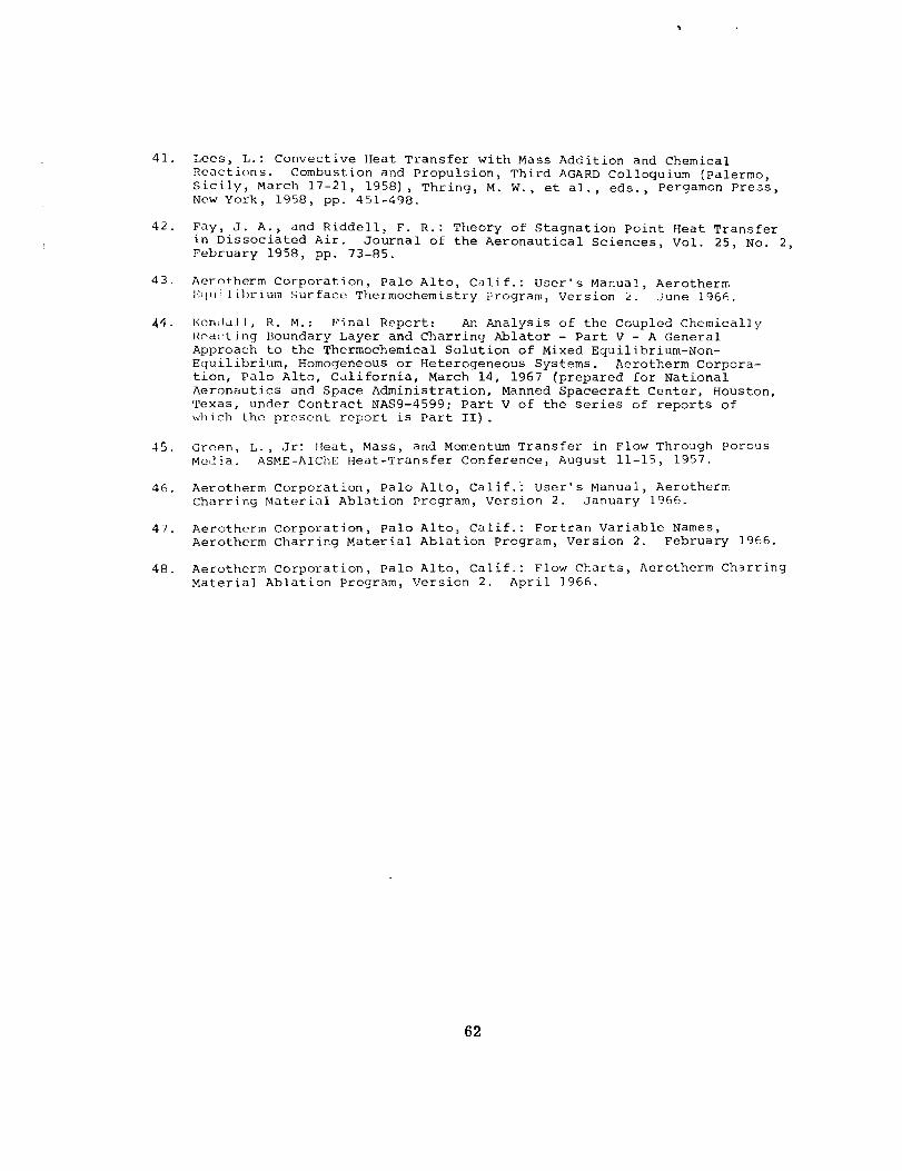
41.

42.

43.

44.

45.

46.

47.

48.

Lees, L.: Convective }{eat Transfer with Mass Addition and Chemical

Reactions. Combustion and Propulsion, Third AGARD Colloquium (palermo,

Sicily, March 17-21, 1958) , Thring, M. W., et al., eds., Pergamon Press,

New York, 1958, pp. 451-498.

Fay, J, A., and Riddell, F. R.: Theory of Stagnation Point Heat Transfer

in Dissociated Air. Journal of the Aeronautical Sciences, Vol. 25, No. 2,

February 1958, pp. 73-85.

Aerotherm Corporations Palo Alto, Calif.: User's Manual, Aerotherm

l_qHi | ibrium Surface Thermochemistry Program, Version 2. June 1966.

Ken_1_:1]l, R. M.: Final Report: An Analysis of the Coupled Chemically

Reacting Boundary Layer and Charring Ablator - Part V - A General

Approach to the Thermochemical Solution of Mixed Equilibrium-Non-

Equilibrium, Homogeneous or Heterogeneous Systems. Aerotherm Corpora-

tion, Palo Alto, California, March 14, 1967 (prepared for National

Aeronautics and Space Administration, Manned Spacecraft Center, Houston,

Texas, under Contract NAS9-4599; Part V of the series of reports of

which the present report is Part II) .

Green_ I,., Jr: Heat, Mass, and Momentum Transfer in Flow Through Porous

Media. ASME-AIChE Heat-Transfer Conference, August 11-15, 1957.

Aerotherm Corporation, Palo Alto, Calif.: User's Manual, Aerotherm

Charring Material Ablation Program, Version 2. January 1966.

Aerotherm Corporation, Palo Alto, Calif.: Fortran Variable Names,

Aerotherm Charring Material Ablation Program, Version 2. February 1966.

Aerotherm Corporation, palo Alto, calif.: Flow Charts, Aerotherm Charring

Material Ablation Program, Version 2. April 1966.

62

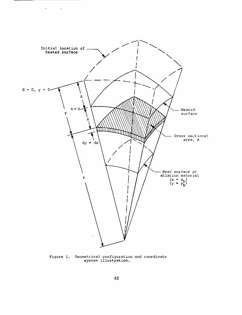
Initial location of__

heated surface

S= 0_ y = 0_

x=

Y

\

//

/

\

\

Heated

surface

dy = dx

/

/

/

Cross sectional

area, A

Rear surface of

ablation material

(y

Figure i. Geometrical configuration and coordinate

system illustration.

63

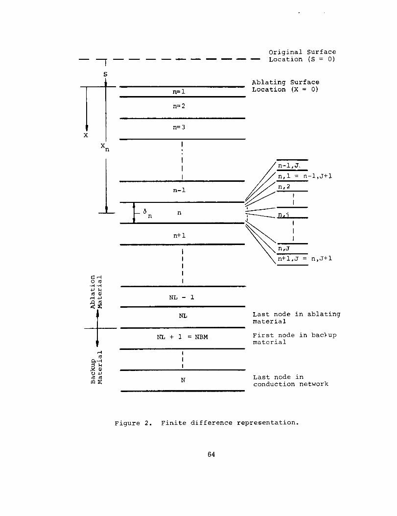
X

Xn

i

o

_4

_4J

mE

n--1

n= 2

n= 3

I

t

I

I

n-i

n

n+l

NL - 1

NL

NL + i = NBM

i

I

i

N

Original Surface

Location (S = 0)

Ablating Surface

Location (X = 0)

n,1 = n-l,J+l

n,2

_ nlj ,

II

n,J

n+l,J = n,J+l

Last node in ablatingmaterial

First node in backupmaterial

Last node in

conduction network

Figure 2. Finite difference representation.

64

65

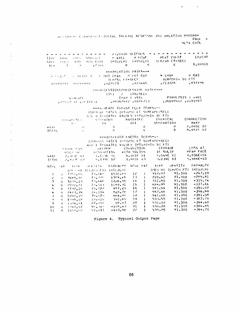
C ln,(_l ''r' r-' lt_.l"l_L I'Ht _ anL _t SPI'_\St-. AI_I) AHLA T T_jN P i_0 G [4A ,,.'

P A_i:_

r.,IL"#+ Et)OL

.............. ; _._loOfl _F Ci"r,ll)% -

C, lr," i It-, 'i-II' ,i,'.iJ (I<_) {_ILJ/L_#) (ttILJ/LH)

---ht.wL.r_l [(]!q t.>AIEI-- -

' ' '' _ ! rlr i !'_'_1''_ I; _' iliIT (]b/IF, "4 I;IJT (_ilS

II.l_/S(; F I-St'C)

.... t_ CI'5F, IC_;7/_t'tTF%SIIH' F,i_Tt:__---

( It,l) I (]NIhF. C)

.a:-,_,_, iI .,,(;.4_),,i .,.,_j4A,-,;a/ .rlnl_f13

---._, _+I-ACE I-:(\I-_,(.4YELL;J( [FHI,,%---

('_I_'"_,,,_I "ATFb (ril'IJ/b(_ F [ S_I'IFAi_I=-_,FC)

',,.,, i, r, _:l_ATt- v_iI_IJLS (_lL]/(}.]t_ S( Q F [)

( fll,vel _FI ,i .4Fill Li rtl) I_Ai}l A [I-I.', Cl-.I-I_ [CAL

I , [wq Llll [ GI-_b I- I-4A[ [ (lr, I

14.,',lt _ f) 0 OIF' I r,l_ ,_ 1) O 0

t _li,ill f'vi%

{.Jf {.]_ i!l -_

i-,_ I i 7'. _#,If- Ill

T("I t_l_ 2. _l,i,r ri4

IxCl_i: ,_t I,- "'l °

I il .1 _(--,.; . i'_i I

( {t t __'4"J . $11

4. 0 ,_q_P. LI

('l )14 2 ,, i _

(', ;i 74 ! 4. tW

# t) ") _'II ,_,. _.t'_

lit i) I J4 t.'-'l 1

11 i) l b_ / ._,>"

flEeT COl! P F CPlCH(q

(I.H/bQ F T-C,EC)

0 ?. 0 (lOll 0

M (.;HAP 14 GAS

(LHIO_Ih S(-) FT)

• / i .]_?_ . H3 #'4'_4

PY_{.iI_YSTS (.'-)8)

,6h6W'4_lt . (ill9| _'-i7

C()Nf)tJC T I t)N

AwAY

P, O_bE O?

H.461E U3

---lr_lr i_ [C,4

_,I-( lii,'l-;

tol,.BE rll

. I _qh Or?

Ft,IEIIGY 1 t'LR.4S---

(i,llll%(; FT Si}_IF_Ct-]-SFt;)

C(Ii,lv#-CT ION _ IIi'IRAGF

wl rtl F,[)LIii% Ih _>tiL[O

h.0#,|F Ill _o54t+E 0l

l._'f,_P ill "i.73#I:_"03

,,_l, _1 !_' t-NII-AIiaY N('hol:: PAT FKvP

(l_p/( ,s P I I (t4Tu/L,_) (iJt;:t; R)

1 !..',_,- 1516.b_ 1_ I "v1 ,'.'-w7

1_. _<_ l=16q.(& I 4 | 8()b.,4.?

( _,')*i _ |ll_'9.]i ]b ] hbaa,9 (4

I_, t?. .a _E/,d"* 16 1 b_al,54

[,-,. 10_ .,_0. t_ It l b% 7.4(..,

7'-_. I 2", he4._'_ IH I b4l.llO

/'J.- lh aJ_0.4.b l"J l b3_'l.b5

_ I, >'_" _ta.V I 7(I 1 '%_|.10

9'_. 4a" - I I)r_. _¢;] ;_1 } b]ii.?O

Ul.lll -lq3.b(" 7,7 1 b Ir).o5

I.()_S AT

_F Ai-i FACE

H.'.)3OE- 04

b. bM,_E-03

I)FI_SITY FNTMALPY

(LN/CU FT) (RTU/LI'J)

til. 3(io -?4l. Oq

91.300 -?VlS.Hl

_I,300 -3lb. 1_

91o300 -337,64

'-)1.300 -35u.07

91.300 -35_._q

9] .3nO -361 .bR

'J] • 3or) -363.(0

(41.300 -364._,0

_1.300 -36_.6%

91,300 -.}6_, I0

Figure 4. Typical Output Page

66

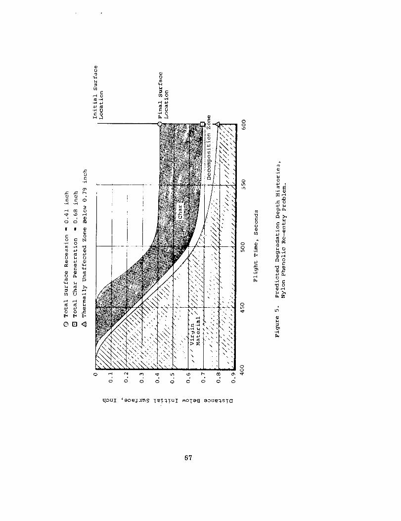
,C ,.C0

._ _o

o,_U U

c0 r-,

""_ 0

r_

U

r.4 ,-_

0 0

@rn

w0

g-I1.4

rll

,-_ 0rO,,_

•'_ 0C 0

0

O_

g

0

Q)c0

0

U

c

f_

,C

<1

t ........

:: ,r," _N'

I_, \ _\\\ \\-"- '

o ,,,-I c,q

o o

Of_q4

_0

C 0'H 0

t.: ." ....

-;r.'_,:Z; _"

\

x• ",, • % N

>:

0 0 0 0

I=

, "?x\ ®

\ "x\

,\,

N

\

• \_i x \ \

_" ,

\

_ t/3

i!] "

2"

%,'%' • 'N _

\\ \ x

\ -

o

g o d

0O

,--4

Ill

0

-,4 _)

_4

0 C"4 111

¢_ II)'t:I_

I11,._

0•,'_ __ 011_,-4

J

IIIl-I

qouI 'eoeixns T_3%3Ul _OTaS aou_%s3_

69

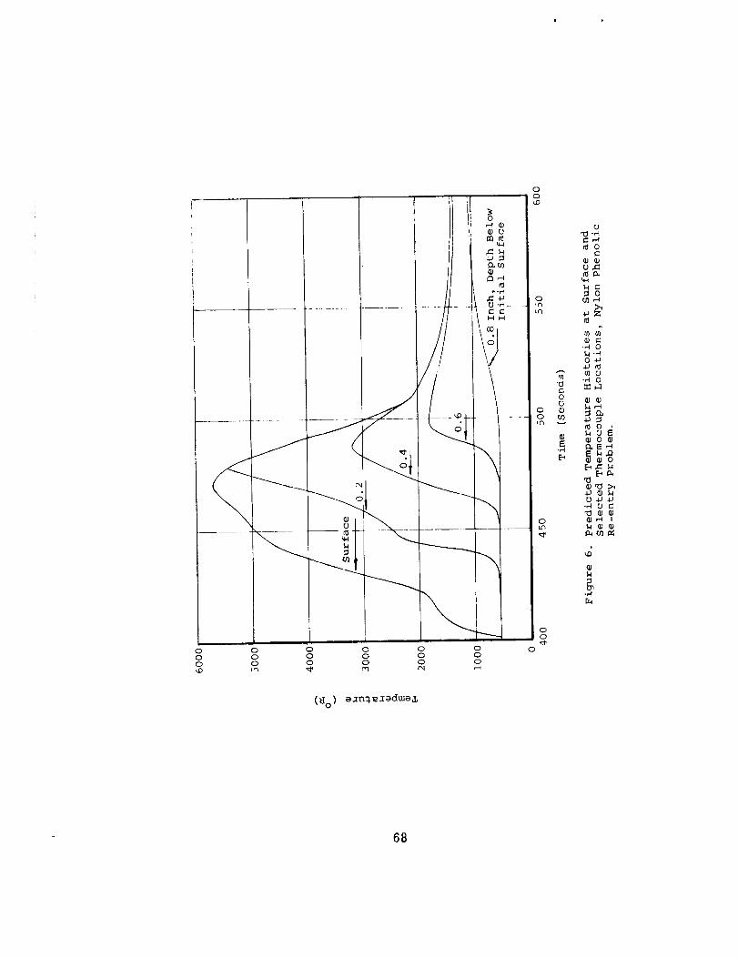
0 0 0 0 0 00 0 0 0 0 00 0 0 0 0 0

(_o) gln_xgd_8_

o

oo

68

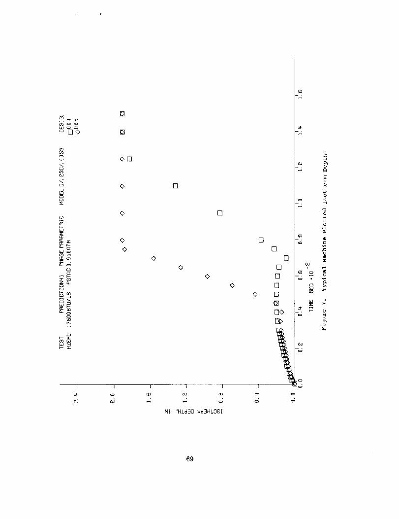
_4

LLJ _ E:_

Q3

<

O3

<O

.J

123

l_J

rr

n rr

n c=_

rr

O3Z nOM

_o

E)I--- rr03 _J

NI-- "r"

I

=t"

[]

[]

<>E]

0 []

0 []

<>

<>

<>

<>

<>

<>

<>

[]

I

cJ

I I I

N[ 'N±d30 W_3Nt0£[

I

[]

[]

[]

=t"0

_XJ

[]

rrl

[]

[]

O

l-l<>[3>"i

d

O

ulH

4-]4J

0

-,'4

0d

_ r..I

N

69

APPENDIX A

EQUATIONS FOR COEFFICIENTS A n , B n, Cn, AND D n

IN IN-DEPTH ENERGY EQUATION ARRAY

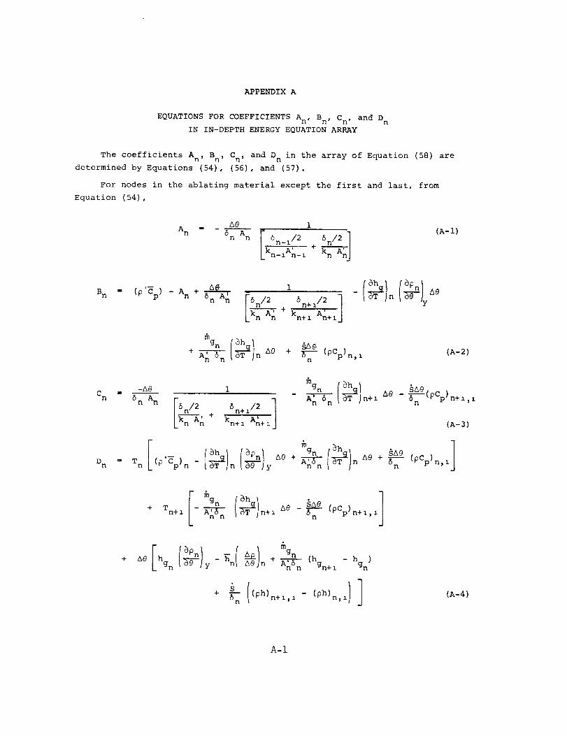
APPENDIXA

EQUATIONSFORCOEFFICIENTSAn, Bn, Cn, and DnIN IN-DEPTHENERGYEQUATIONARRAY

The coefficients An, Bn, Cn, and D n in the array of Equation (58) are

determined by Equations (54), (56), and (57).

For nodes in the ablating material except the first and last, from

Equation (54),

Ae 1

k n-l n-I kn An]

B n

n n

6n/2 _n+i/2 ]_--_r + A'n n kn+ z n+ 1

+ A n 6------_ n A0 + (pCp)n, ln

(A-2)

Cn

-Ae

6 n A n

6 n/2 6 ]_--_, + n+zA/_

n n kn+ z n+ i

- _ n+1 Ae - _-_n _p pln+z,_n n

(A-3)

D n = T n

+ Tn+ z - n+ 1

[_o{_)__o{_)n+_non(_+__n_Ae

+ q (Ph)n+l, 1 n,z(A-4)

A-I

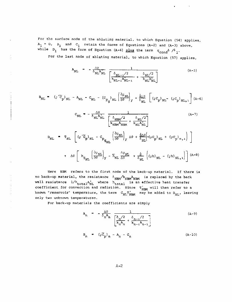
For the surface node of the ablating material, to which Equation (54) applies,

A 1 = 0, B 1 and C 1 retain the forms of Equations (A-2) and (A-3) above,

while D 1 has the form of Equation (A-4) plus the term qcond A /61.

For the last node of ablating material, to which Equation (57) applies,

40

ANL 6NLANL

6NL/26NL-I/2 +

kNL-IANL-I kNLANL J

(A-5)

-- _ 2 I(pCp) (pCp) 1] (A-6)BNL = (p'Cp)NL - ANL - CNL - (Cpg)NL {_)y 6NL NL- NL,

Ae 1 (A-7)

DNL " _NL (_p)NL - CpgN_ Ie_----Jy_e + _NLI-_CP)N_ (_CP)n'

[ I I I]A8+ Ae hgNL e_'--Jy - hNL A0 + --6NL (Ph)NL - NL, I

Here NBM refers to the first node of the back-up material. If there is

no back-up material, the resistance 6NBM/kNBMANB M is replaced by the back

hwall resistance i/ totalANL where htota I is an effective heat transfer

coefficient for convection and radiation. Since T_BM_ will then refer to a

known "reservoir" temperature, the term CNLT_B M may be added to DNL _ leaving

only two unknown temperatures.

For back-up materials the coefficients are simply

40 i

An 6 A (A-9)

n n _6n/____2 6n-1/2 1LknA n + kn_lAn_m

Bn = (pCp)n - An - Cn (A-10)

A-2

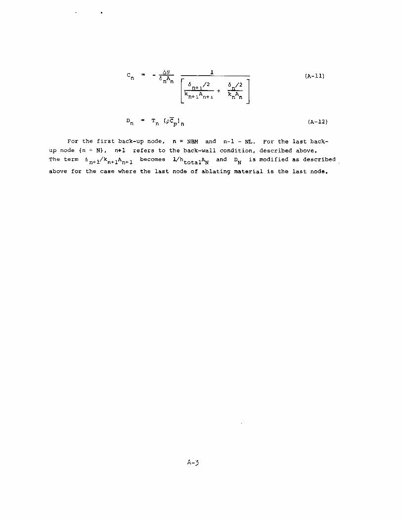
ae i (A-ll)

Cn = 6nAn [ 6n+i/2 6n/2 l

Lkn+ iAn+ l + knAn J

Dn = Tn (P_p) n (A-12)

For the first back-up node, n = NBM and n-i - NL. For the last back-

up node (n = N), n+l refers to the back-wall condition, described above.

The term 6n+i/kn+iAn+ 1 becomes I/htotalA N and D N is modified as described

above for the case where the last node of ablating material is the last node.

A-3

APPENDIX B

CONDUCTION SOLUTION CHECK-OUT

OF THE CHARRING MATERIAL ABLATION PROGRAM

PRECEDING PAGE BLANK NOT FILMED.

TABLE OF CONTENTS

Appendix B

List of Symbols for Appendix B

B.I INTRODUCTION

B.2 ASPECTS OF PROGRAM

B.3 CONSTANT PROPERTIES SLAB

B.4 CONSTANT PROPERTIES CYLINDER

B.5 CONSTANT PROPERTIES SPHERE

B.6 SEMI-INFINITE SOLID WITH CONSTANT PROPERTIES

B.7 SEMI-INFINITE SOLID WITH VARIABLE THERMAL CONDUCTIVITY

B.8 SEMI-INFINITE RECEDING SOLID

B.9 SUMMARY AND CONCLUSIONS

REFERENCES

FIGURES

SUB-APPENDIX B-I ERROR ANALYSIS OF STEADY STATE SOLUTION FOR

A CONSTANT PROPERTIES SEMI-INFINITE RECEDING

SOLID WITH CONSTANT SURFACE TEMPERATURE AND

CONSTANT SURFACE RECESSION RATE

v

B-I

B-I

B-I

B-2

B-3

B-4

B-5

B-7

B-9

B-10

B-I-I

iii

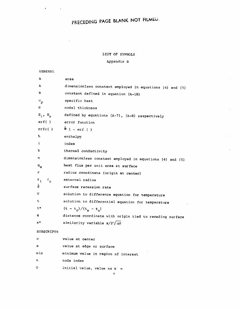
PKECEDING PAGE BLANK NOT FII._ELJ.

GENERAL

A

A

B

cP

d

E 1 _ E_,

erf( )

erfc ( )

h

i

k

n

qe

r

r r1 e

T

t

t*

x

x*

SUBSCRIPTS

c

e

min

n

0

LIST OF SYMBOLS

Appendix B

area

dimensionless constant employed in equations (4) and (5)

constant defined in equation (A-18)

specific heat

nodal thickness

defined by equations (A-7), (A-8) respectively

error function

_ 1 - erf ( )

enthalpy

index

thermal conductivity

dimensionless constant employed in equations (4) and (5)

heat flux per unit area at surface

radius coordinate (origin at center)

external radius

surface recession rate

solution to difference equation for temperature

solution to differential equation for temperature

(t - to)/(t e - t o )

distance coordinate with origin tied to receding surface

similarity variable x/2_

value at center

value at edge or surface

minimum value in region of interest

node index

initial value, value as x

v

GREEK

c_

6

6

e

SPECIAL

z

--i

thermal diffusivity k/pCp

arithmetic error

time increment

slab thickness

error T* - t*

time

equal to by definition

approximately equal to

vi

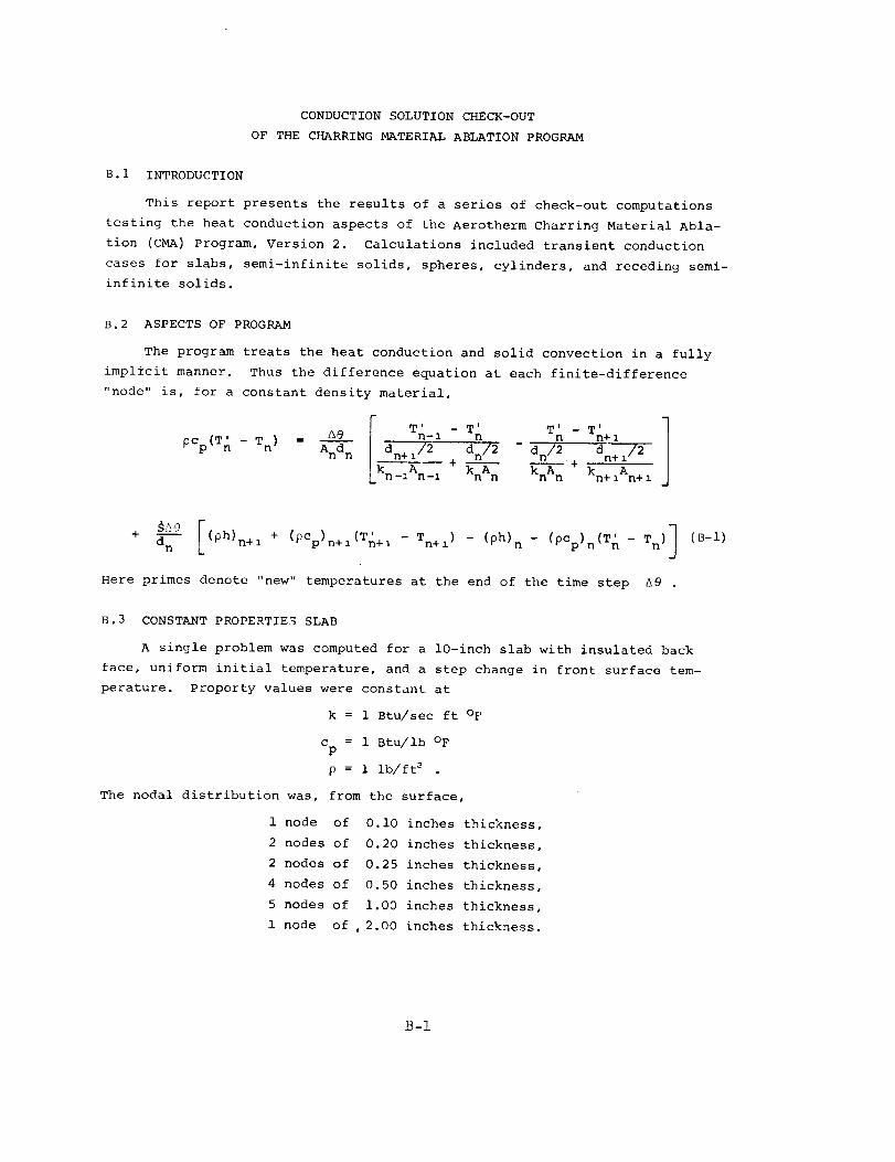
CONDUCTION SOLUTION CHECK-OUT

OF THE CHARRING MATERIAL ABLATION PROGRAM

B.I INTRODUCTION

This report presents the results of a series of check-out computations

testing the heat conduction aspects of the Aerotherm Charring Material Abla-

tion (CMA) Program, Version 2. Calculations included transient conduction

cases for slabs, semi-infinite solids, spheres, cylinders, and receding semi-

infinite solids.

B.2 ASPECTS OF PROGRAM

The program treats the heat conduction and solid convection in a fully

impl_cit manner. Thus the difference equation at each finite-difference

"node" is, for a constant density material,

I T' - T' T' - T'

Ae n- 1 n n n+ 1

pCp (T n - Tn) Andn dn+ i/2 dn/2 _ dn/2 dn+ i/2__ +

Lkn-lAn-1 +knAn knAn kn+ 1An+ 1

+d n (Ph)n+ 1 + (pCp)n+l(Tn+1 - Tn+ l) - (ph) n - (pCp)n(Tn - Tn) I (B-l)

Here primes denote "new" temperatures at the end of the time step be

B.3 CONSTANT PROPERTIE_ SLAB

A single problem was computed for a 10-inch slab with insulated back

face, uniform initial temperature, and a step change in front surface tem-

perature. Property values were constant at

k = 1 Btu/sec ft OF

c = 1 Btu/ib OFP

p = 1 ib/ft 3

The nodal distribution was, from the surface,

1 node of

2 nodes of

2 nodes of

4 nodes of

5 nodes of

1 node of

0.I0 inches thicknes_

0.20 inches thickness

0.25 inches thickness

0.50 inches thickness

1.00 inches thickness

2.00 inches thickness

B-I

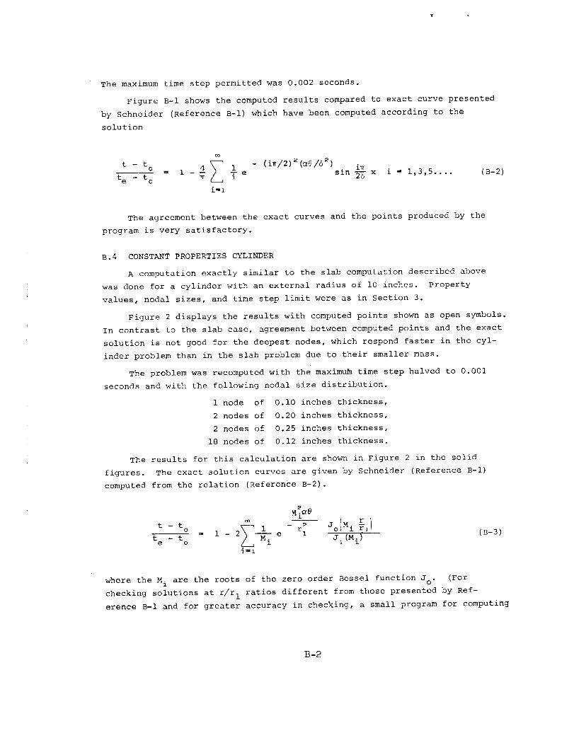
The maximum time step permitted was 0.002 seconds.

Figure B-I shows the computed results compared to exact curve presented

by Schneider (Reference B-l) which have been computed according to the

solution

t - t O w 1 4 _. 1 - (i_/2)2(_@/62) ivt e - t o - _ T e sin _- x

i = 1,3,5 .... (B-2)

The agreement between the exact curves and the points produced by the

program is very satisfactory.

B.4 CONSTANT PROPERTIES CYLINDER

A computation exactly similar to the slab computation described above

was done for a cylinder with an external radius of i0 inches. Property

values, nodal sizes, and time step limit were as in Section 3.

Figure 2 displays the results with computed points shown as open symbols.

In contrast to the slab case, agreement between computed points and the exact

solution is not good for the deepest nodes, which respond faster in the cyl-

inder problem than in the slab problem due to their smaller mass.

The problem was recomputed with the maximum time step halved to 0.001

seconds and with the following nodal size distribution.

1 node of 0.i0 inches thickness,

2 nodes of 0.20 inches thickness,

2 nodes of 0.25 inches thickness,

18 nodes of 0.12 inches thickness.

The results for this calculation are shown in Figure 2 in the solid

figures. The exact solution curves are given by Schneider (Reference B-l)

computed from the relation (Reference B-2).

I rl1 r 0t-t° = 1-2 --M-?e I j )

te - to 1 i (Mi

i_l

(B-3)

where the M i are the roots of the zero order Bessel function Jo" (For

checking solutions at r/r I ratios different from those presented by Ref-

erence B-I and for greater accuracy in checking, a small program for computing

B-2

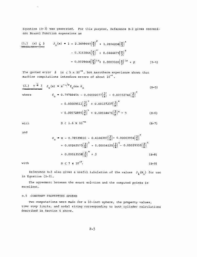
Equation (B-3) was generated. For this purpose, Reference B-3 gives conveni-

ent Bessel Function expansions as

(i.) (x) _ 3 Jo(x) - 1 - 2.2499997 + 1.2656208 7

- 0. 3163866(3) _ + 0.0444479(3) s

- 0.0039444[_)io+ 0. 0003100( _] i_ + (B-4)

The quoted error _ is < 5 x i0 -e , but Aerotherm experience shows that

machine computations introduce errors of about 10 -7 .

(2.) x _ 3 J (x) _ x-i/_f cos 8o o o

wherefo = 0. 79788456-0.00000077 xj - 0.00552740

000072895( )5 000014,76( )°

(B-5)

(B-6)

with _ < 1.6 x i0 -s (B-7)

and

ao (3)= x - 0.78539816 - 0.4166397 x - 0.00003954

+ 0.00262573[3) 3 - 0.00054125(3) 4- 0.00029333(3) 5

ooool3ss ( ) (B-S)

with B < 7 x i0 -s (B-9)

Reference B-3 also gives a useful tabulation of the values Jl(Mi) for use

in Equation (B-3).

The agreement between the exact solution and the computed points is

excellent.

B.5 CONSTANT PROPERTIES SPHERE

Two computations were made for a 10-inch sphere, the property values,

time step limits, and nodal sizing corresponding to bothcylinder calculations

described in Section 4 above.

B-5

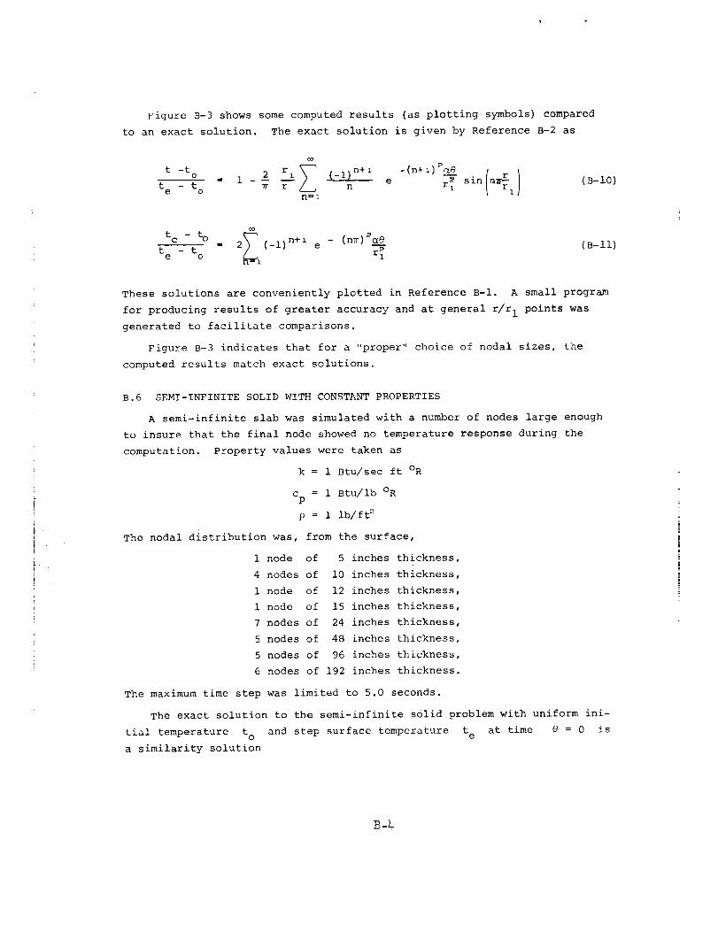
Figure S-3 shows some computed results (as plotting symbols) compared

to an exact solution. The exact solution is given by Reference B-2 as

oo

t-to 1 2 rl_ (-l)n+l - (n+ i) _69 ( r )t e - t o T[ V n e r_ sin aT;_ln_l

(B-10)

o0

tc - to 2_l(-l)n+l e - (nTr)_-c_8t e - t o r_(B-II)

These solutions are conveniently plotted in Reference B-I. A small program

for producing results of greater accuracy and at general r/r I points was

generated to facilitate comparisons.

Figure B-3 indicates that for a "proper" choice of nodal sizes, the

computed results match exact solutions.

|

L

B.6 SEMI-INFINITE SOLID WITH CONSTANT PROPERTIES

A semi-infinite slab was simulated with a number of nodes large enough

to insure that the final node showed no temperature response during the

computation. Property values were taken as

k = 1 Btu/sec ft OR

c = 1 Btu/ib ORP

p = 1 ib/ft 2

The nodal distribution was, from the surface,

1 node of

4 nodes of

1 node of

1 node of

7 nodes of

5 nodes of

5 nodes of

5 inches thickness

i0 inches thickness

12 inches thickness

15 inches thickness

24 inches thickness

48 inches thickness

96 inches thickness

6 nodes of 192 inches thickness

The maximum time step was limited to 5.0 seconds.

The exact solution to the semi-infinite solid problem with uniform ini-

tial temperature t o and step surface temperature t e at time 8 = 0 is

a similarity solution

B-4

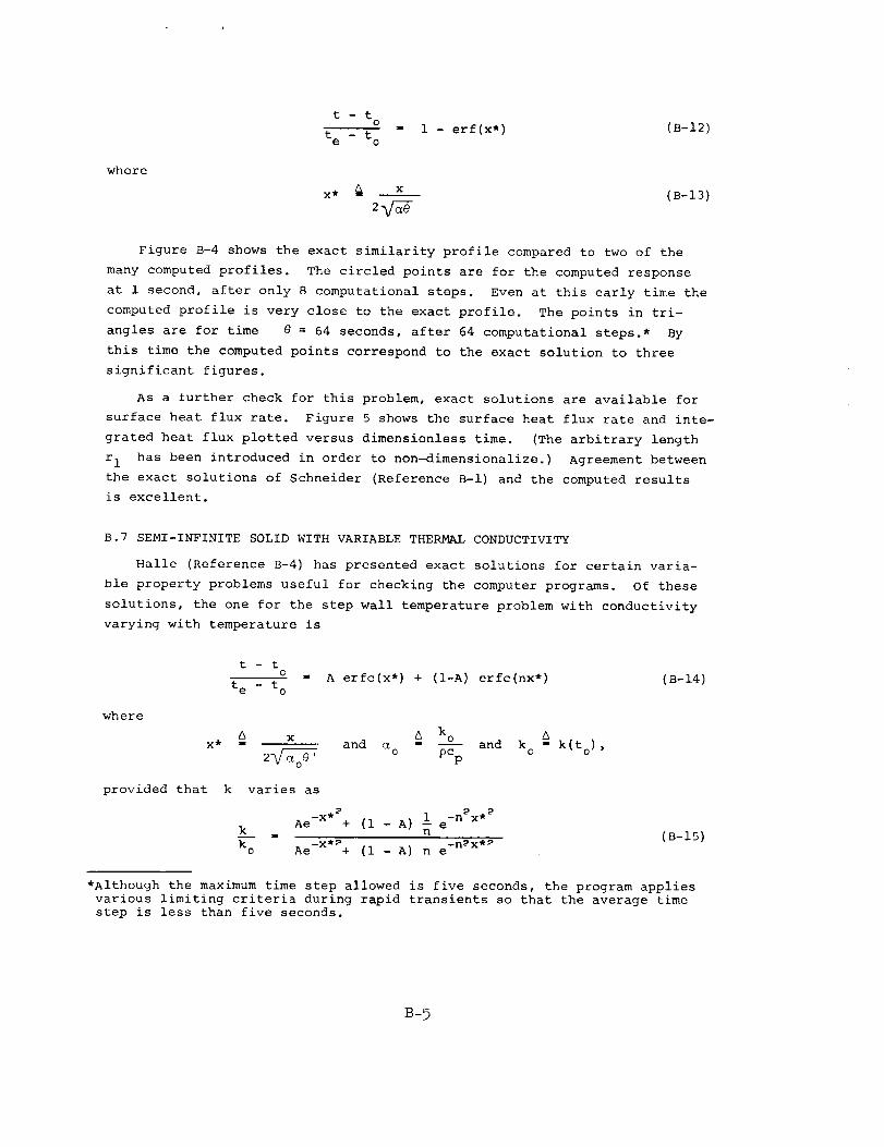
where

t - to

- 1 - erf(x*) (B-12)t - te o

x* _ x (B-13)

Figure B-4 shows the exact similarity profile compared to two of the

many computed profiles. The circled points are for the computed response

at 1 second, after only 8 computational steps. Even at this early time the

computed profile is very close to the exact profile. The points in tri-

angles are for time e = 64 seconds, after 64 computational steps.* By

this time the computed points correspond to the exact solution to three

significant figures.

As a further check for this problem, exact solutions are available for

surface heat flux rate. Figure 5 shows the surface heat flux rate and inte-

grated heat flux plotted versus dimensionless time. (The arbitrary length

r I has been introduced in order to non-dimensionalize.) Agreement between

the exact solutions of Schneider (Reference B-l) and the computed results

is excellent.

B.7 SEMI-INFINITE SOLID WITH VARIABLE THERMAL CONDUCTIVITY

Halle (Reference B-4) has presented exact solutions for certain varia-

ble property problems useful for checking the computer programs. Of these

solutions, the one for the step wall temperature problem with conductivity

varying with temperature is

t - to

t e - t o" A erfc(x*) + (l-A) erfc(nx*) (B-14)

where

A x Zi k O

and _ - and k ° g k(t o) ,x* - 2_e0 e , o 9Cp

provided that k varies as

Ae-X .2 1 -nPx *Pk . + (i -A) we-- -n_x*_ (B-15)ko Ae-X*_+ (i - A) n e

*Although the maximum time step allowed is five seconds, the program applies

various limiting criteria during rapid transients so that the average time

step is less than five seconds.

B-5

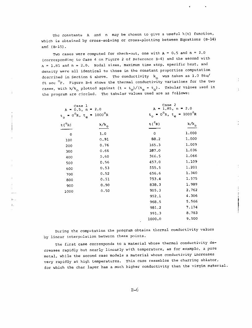
The constants A and n may be chosen to give a useful k(t) function,

which is obtained by cross-solving or cross-plotting between Equations (B-14)

and (B-15).

Two cases were computed for check-out, one with A = 0.5 and n = 2.0

(corresponding to Case 4 on Figure 2 of Reference B-4) and the second with

A = 1.85 and n = 2.0. Nodal sizes, maximum time step, specific heat, and

density were all identical to those in the constant properties computation

described in Section 6 above. The conductivity k ° was taken as 1.0 Btu/

ft sec oF. Figure B-6 shows the thermal conductivity variations for the two

cases, with k/k ° plotted against (t - to)/(t e - to). Tabular values used in

the program are circled. The tabular values used are as follows:

Case 1

A _ 0.5, n - 2.0

t I O°R, t I IO00°R0 e

t (OR) k/k o

0 1.0

i00 0.91

200 0.76

300 0.66

400 0.60

500 0.56

600 0.53

700 0.52

800 0.51

900 0.50

i000 0.50

Case 2

A I 1.85, n = 2.0

t o = 0°R, t e

t(°R)

0

88.2

165.3

287.0

366 5

457 0

555 5

656 6

753 4

838 3

905 3

952 1

968 5

981 2

991 3

i000.0

=, lO00°R

k/k o

1.000

1.000

1.009

1.036

1.066

I. 109

1.201

1. 340

1.575

1.989

2.762

4.306

5.566

7. 174

8.783

9. 500

During the computation the program obtains thermal conductivity values

by linear interpolation between these points.

The first case corresponds to a material whose thermal conductivity de-

creases rapidly but nearly linearly with temperature, as for example, a pure

metal, while the second case models a material whose conductivity increases

very rapidly at high temperatures. This case resembles the charring ablator,

for which the char layer has a much higher conductivity than the virgin material.

B-6

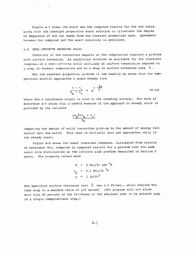
Figure B-7 shows the exact and the computed results for the two cases,

along with the constant properties exact solution to illustrate the degree

of departure of the two cases from the constant properties case. Agreement

between the computed and the exact solutions is excellent.

B.8 SEMI-INFINITE RECEDING SOLID

Check-out of the convection aspects of the computation requires a problem

with surface recession. An analytical solution is available for the transient

response of a semi-infinite solid initially at uniform temperature exposed to

a step in surface temperature and to a step in surface recession rate S .

For the constant p_operties problem it can readily be shown that the tem-

perature profile approaches a quasi-steady form

t - t Sx

o . e _ (B-16)t - te o

where the x coordinate origin is tied to the receding surface. The work of

Reference B-5 shows that a useful measure of the approach to steady state is

provided by the variable

pcps (t e - t o)

qe

comparing the amount of solid convection pick-up to the amount of energy con-

ducted into the solid. This term is initially zero and approaches unity in

the steady state.

Figure B-8 shows the exact transient response, calculated from results

of Reference B-5, compared to computed results for a problem with the same

nodal size distribution as the infinite slab problem described in Section 6

above. The property values were

k = 1 Btu/ft sec OF

c = 0.i Btu/ib OFP

p = 1 Ib/ft 3

The specified surface recession rate S was 0.5 ft/sec., which limited the

time step to a maximum value of 1/6 second. (The program will not allow

more than 20 percent of the thickness of the smallest node to be ablated away

in a single computational step.)

B-7

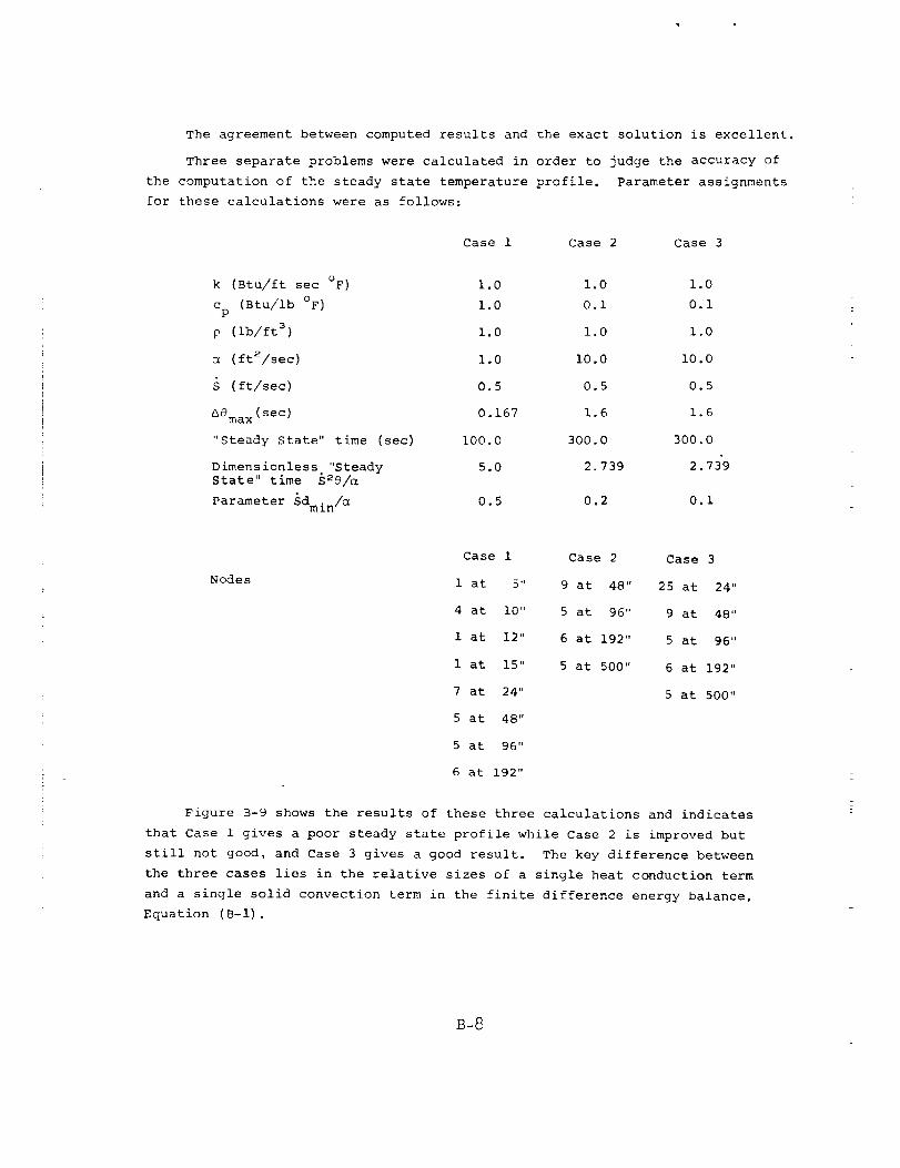
The agreement between computed results and the exact solution is excellent.

Three separate problems were calculated in order to judge the accuracy of

the computation of the steady state temperature profile. Parameter assignments

for these calculations were as follows:

Case 1 Case 2 Case 3

k (Btu/ft sec OF) 1.0 1.0 1.0

c (Btu/ib OF) 1.0 0.i 0.iP

p (ib/ft 3) 1.0 1.0 1.0

(ft2/sec) 1.0 i0.0 i0.0

(ft/sec) 0.5 0.5 0.5

A_max(Sec) 0.167 1.6 1.6

"Steady State" time (sec) i00.0 300.0 300.0

Dimensionless "Steady 5.0 2.739 2.7{9

State" time S2e/_

Parameter Sdmin/_ 0.5 0.2 0.i

Nodes

Case 1

1 at 5"

4 at i0"

1 at 12"

1 at 15"

7 at 24"

5 at 48"

5 at 96"

6 at 192"

Case 2 Case 3

9 at 48" 25 at 24"

5 at 96" 9 at 48"

6 at 192" 5 at 96"

5 at 500" 6 at 192"

5 at 500"

Figure B-9 shows the results of these three calculations and indicates

that Case 1 gives a poor steady state profile while Case 2 is improved but

still not good, and Case 3 gives a good result. The key difference between

the three cases lies in the relative sizes of a single heat conduction term

and a single solid convection term in the finite difference energy balance,

Equation (B-l).

B-8

conduction term = kd (Tn+1 - Tn)

convection termpCp S (Tn+ l - Tn)

convection term = _ = S d

conduction term k

(B-17)

(B-IS)

(B-19)

The value of this parameter for dmi n is given in the table above.

Thus Figure B-9 suggests that an accurate calculation requires

_dmin

< 0.i .CZ

(B-20)

It cad be shown through an analysis of truncation errors (see Sub-Appendix B--I)

that this conclusion is no___tgenerally valid. It holds only if

i. The nodes are small enough that truncation errors in the

conduction terms are "small,"

2. The temperature profile is "close" to e -_x/e.

Even though the criterion (B-20) is not generally valid, it is still a

useful one since many ablation problems approximately satisfy the two conditions

B.9 SUMMARY AND CONCLUSIONS

The purpose of the test calculations was to show that the Aerotherm

Charring Material Ablation (CMA) Program, Version 2 (Implicit) performs heat

conduction calculations properly. Checks included computations for slab,

cylinder, spherical, and semi-infinite solid geometries exposed to step sur-

face temperature increases and several calculations of semi-infinite solid

geometries exposed to simultaneous steps in surface temperatures and surface

recession rate.

Results indicated that when nodes were sized properly, the results gen-

erated by the program matched exact solutions and that, therefore, the program

is judged to operate properly in its heat conduction and solid convection

aspects.

Poor choices of node sizes can of course lead to unsatisfactory results,

but a complete analysis of this subject is outside the intended scope of this

appendix.

B-9

REFERENCES

B-1

IF2

1:;-3

P,-4

P,-5

Schneider, P. J.: Temperature Response Charts. John Wiley and Sons,

Inc., New York, 1963.

Schneider, P. J.: conduction IIeat Transfer. Addison-Wesley Publishing

Company, Inc., Cambridge, Massachusetts, 1955, pp. 238-239.

Al)ramowitz, M., and Stegun, I. A., eds.: IIandbook of Mathematical

Functions. National l_ureau of Standards, Applied Mathematics Series

No. 55, United States Government Printing office, Washington, D. C.,

1964, pp. 369-370.

ttalle, If.: Exact Solution of Elementary Transient Heat Conduction

Problem Involving Temperature Dependent Properties. Transactions of

the American Society of Mechanical Engineers, Series C, Journal of

Heat Transfer, vol. 87, No. 3, August 1965, pp. 420-421.

l_aer, D., and Ambrosio, A., Heat Conduction in a Semi-Infinite Slab

With Sublimation at the Surface. Space Technology Laboratories, Inc.,

Pasadena, California, TR-59-0000-00610, February 24, 1959.

I:LPI

L

B-!O

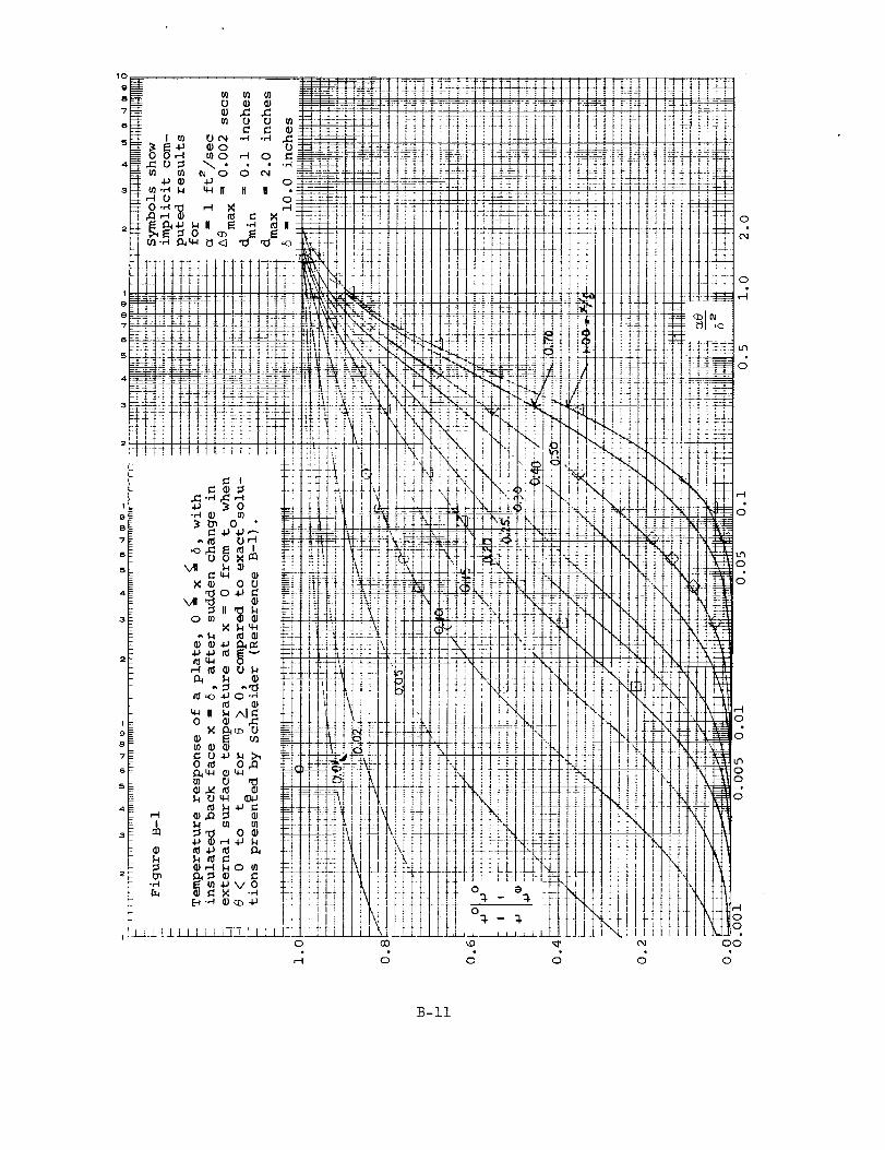
O_

0

B-II

_D

0

,@

0 J

0

0

o

o

0

0

0

o

00

oJ0

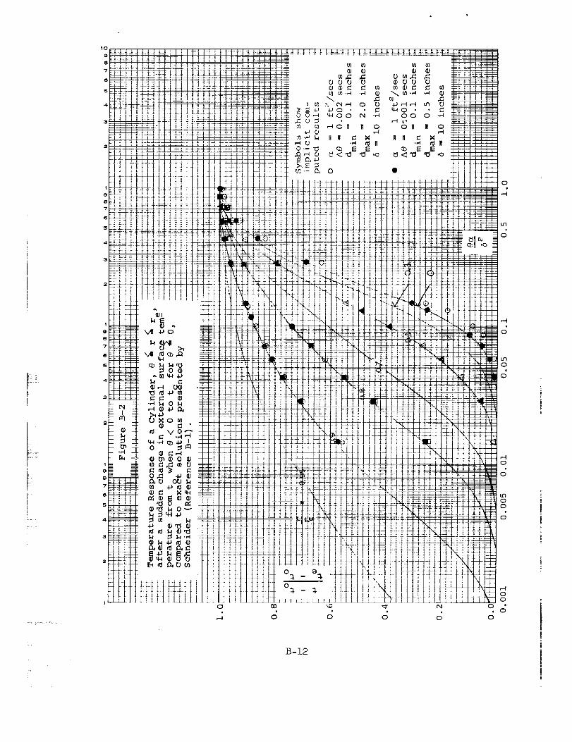
I!!::!,t

!

[

R

:--:L L:r £ =

=

B-12

!4I 1

0

0

0

q_o

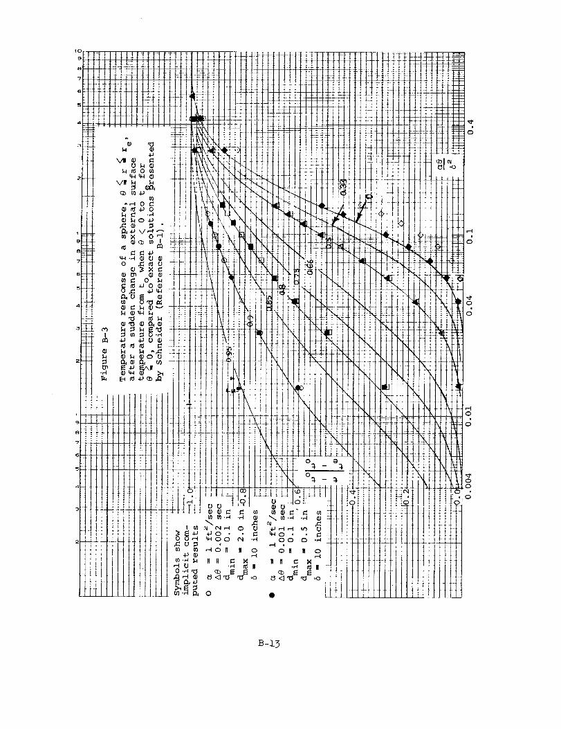
o

B-15

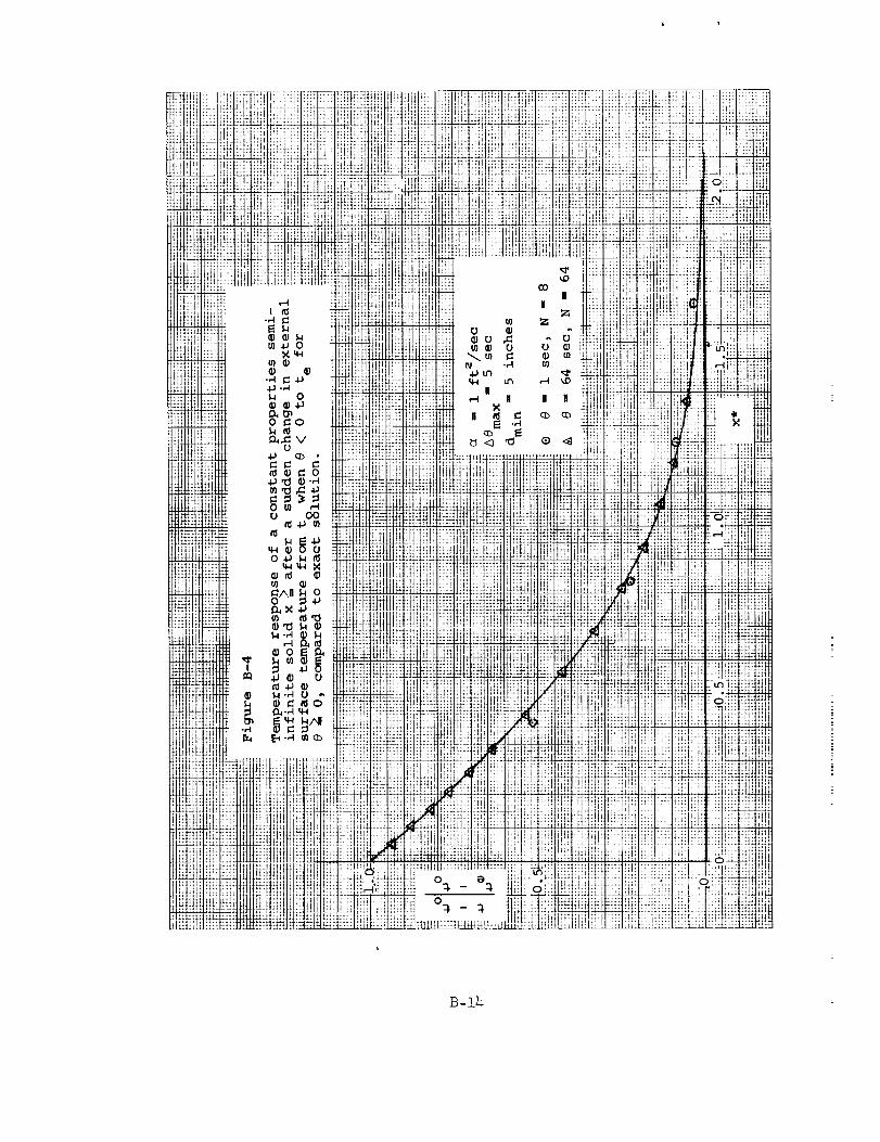
:i[ 7_

!i Y

U

ii iEd[ H:)i 4i

Lq H

:H :i

iiliSH! !FiJ; _t

m i!I

!I) :"

H_

H_ H[H_ H_

HI H:

,. _qj"' !Hi:aill

m i!i

ii i!]

ii H!

t! lilt! _i_

i1N HJl !t

J!iJ_ii!:

!! !!

,_ r

iii!

)_!7l

• ;:i i,!i mF ,% _,,,

:IHII[(Ill:II !:,1i!!:!_'L:_

[_q,_l!;H

)l)il......._i[;Jl

!_/_H¢iH]iHu; .....

;]i!]ili ]::)I

_)i !¢: t

:_!i_]H: i]

¢';7!i11':!$i

i-i _ti!_i?ti?!)

_H........

r t _41+' _j,_lj .I,

_±i ::::IxA;

• t ..... +--1)

NI i!:T _:

iil! .... ' ....ii_ -+, lliil!i :,

....

:_;:iiiiWi

B-14

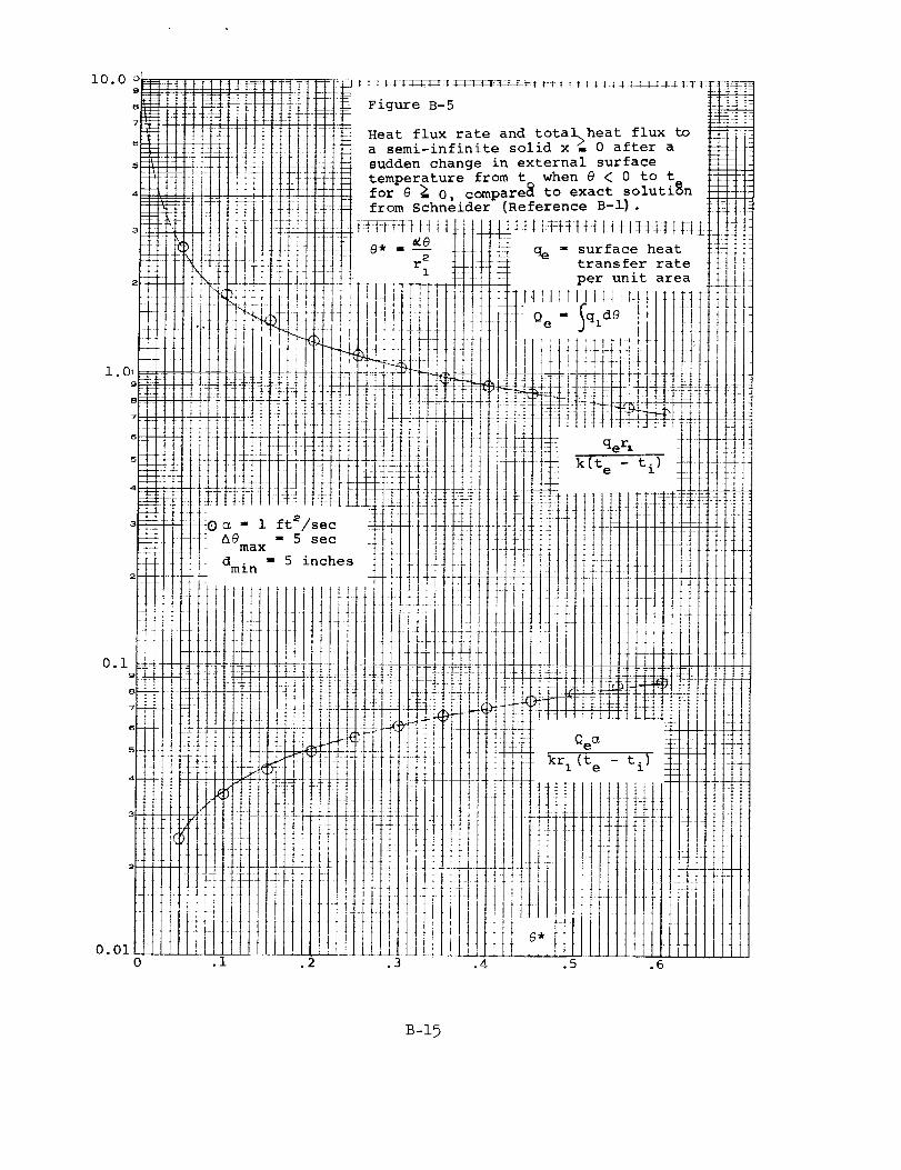
i0.0

0.010

_ 1 ft2/sec

dema x - 5 sec

mdmi n 5 inches

Figure B-5

Heat flux rate and total_heat flux toa semi-infinite solid x _, 0 after a

sudden change in external surface

temperature from t when e < 0 to t

for 8 _ 0, compare_ to exact solutionfrom Schneider (Reference B-_ .

t t t tTH:t _T[.._7_:t t t f t]:.

qe " surface heattransfer rate

per unit area

T_ Lt_:I H :1I i i

qer,

k(t e - ti)

Qe _

kr I (t e - ti)

II!:l

4_4

-_ i +

•+ !

-I-t?

" ]

B-15

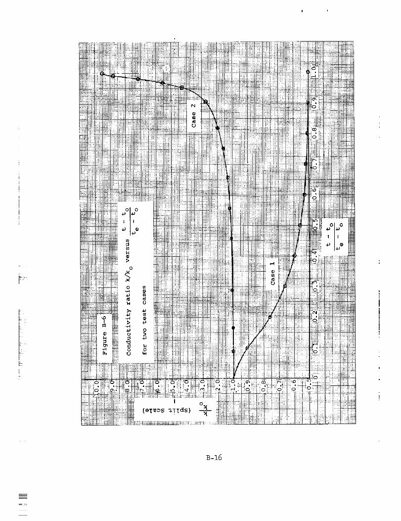
[;F _

!F

B-16

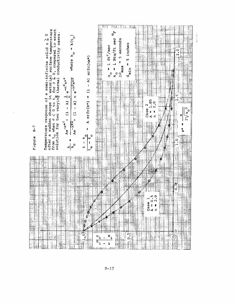
B-Z7

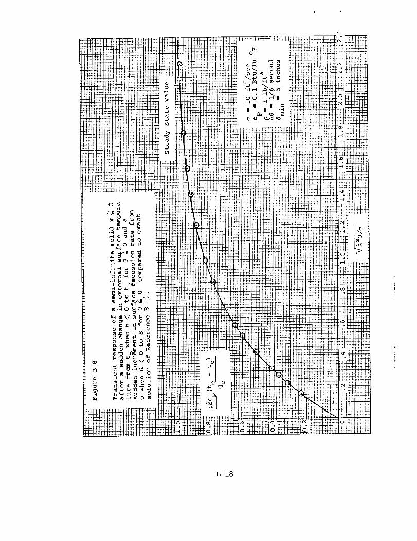
lliiiHH Hi_

i _i!i__ _ _ _..........:I_I i_t _ :i_

IJItIM:

tfr h_n_.t

:

,-.I

@:

:

m i

N

.O t

bt HLLIt:4÷+_

HHII_,fl

H_t_f_

_H_

.tt:_4

_:_

:.:::.:

H_

UH

H+i

_m

iitlHtt

_5

;HI<i!

rl

Hu

r_Hh

lil_

4_

!t!:

T!l:

LLLH_

hid

II5_H

k' LLL ilia! + : _ ]111 tltltlHllHIH_i:i

_MHLL :_1 _2 :II_.J,_HI '. _X!l:ll tiili

_._ _Q.

lit!i!

t

B-18

®

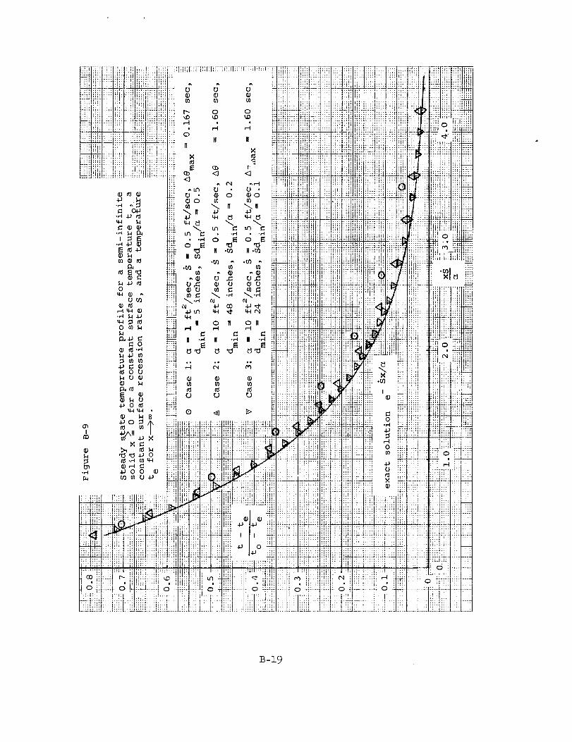
B-19

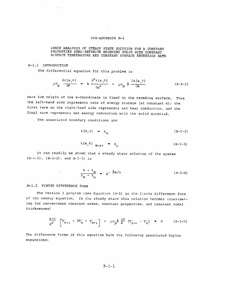
SUB-APPENDIXB-I

ERRORANALYSISOFSTEADYSTATESOLUTIONFORA CONSTANTPROPERTIESSEMI-INFINITERECEDINGSOLIDWITHCONSTANTSURFACETEMPERATUREANDCONSTANTSURFACERECESSIONRATE

B-I.I INTRODUCTIONThe differential equation for this problem is

_t(x,_) _t(x e) _t(x e)

?Cp _ -- k + _ __ (B-l-l)_x _ _ep _x

Here the origin of the x-coordinate is fixed to the receding surface. Thus

the left-hand side represents rate of energy storage (at constant x) ; the

first term on the right-hand side represents net heat conduction, and the

final term represents net energy convection with the solid material.

The associated boundary conditions are

t(0,_) = t e (B-I-2)

t(x 6) - t (s-l-3), X--_ O

It can readily be shown that a steady state solution of the system

(B-l-l), (B-I-2), and B-I-3) is

t - to - §x/_" e

t - te o

(B-I-4)

B-I.2 FINITE DIFFERENCE FORM

The Version 2 program uses Equation (B-I) as the finite difference form

of the energy equation. In the steady state this relation becomes (consider-

ing for convenience constant areas, constant properties, and constant nodal

thicknesses)

(B-I-5)

The difference forms in this equation have the following associated Taylor

expansions:

B-l-1

T(x + d) - 2T(x) + T(x-d)_ - _2T(x) +d _ dx 2

d a _4T(x) + O(d 4) " E

12 8x 4 i

(B-I-6)

T(x + d)- T(x) = _ + d 0_T(x) + O(d _) = E (B-I-7)d dx 2 _ _

OX

Truncating the Taylor series expansions after the second term in both cases

gives, for the two expansions,

= d 2 d4T(xl)E d_T (x) + (B-I-8)

I dx _ 12 dx 4

where

E = dT(x) ÷ d d_T(x_) (B-I-9)dx 2 dx _

x - d _ x _ x + d (B-I-10)

and

x _- x _ x + d (B-I-II)2

Now the original differential equation for the steady state profile is

kd_t

pepS dt+ h-_ " 0dx _

(B-I-12)

or

dtd_t + _-_ 0 (B-I-13)dx _

From Equation (B-I-13) may be derived the useful relation

d4t I'SI 3 d__tt (B-I-14)

dx 4 _J dx

Now if T _ t, these relations may be employed t_ simplify the expansions.

Substitution of (B-I-14) into (B-I-8) and (B-I-13) into (B-I-9) gives

El = dx 2 12 dx

(B-I-15)

_- dT(x) d (_)dT(x2) (B-I-16)E2 dx - _ dx

B-I-2

J

B-I.3 ESTIMATION OF ERROR

Equations (B-l-5), (B-I-7), (B-I-7), (B-l-15), and (B-l-16) imply that

the solution to the difference equation corresponds to a solution of the

differential relation

---_kd_T + pep; dT I kd_ dx 7d _ dT(x )]+ pCpS {_ = 0 (B-I-17)

If d is small, then x I _ x 2 _ x, and so an approximate solution to this

equation and its associated boundary conditions is

Sx BxT - T --- + --

T - o _ e _ _ (B-I-18)

T e - T O

where

Since

then generally

_xsx[_(_)___I]g-" 7- Y_ -- +_" a'- ' (B-I-20)

Bk S_x = 1 and Sd (B-I-21)_-- < < 1 if e _-- < < 1

so that the approximate solution is nearly

Sx

T-- I (B-I-22)

Since e -_x/a is the true solution, the relative error of the approximate

solution is Bx/k, or

_.t._t._._x._x[_(_I_-•_(_I](__'For the relative error to be small, the parameter Sd/% must be small. In

this case, the relative error is given by

B-I-3

(B-1-24)

It is interesting to note that this expression very closely predicts the

error magnitudes for the three cases shown in Figure B-8.*

B-I.4 CONCLUSION

The discussion has shown that errors in the steady state profile of the

constant properties semi-infinite receding solid with constant surface tem-

perature and constant recession rate are given by Equation (B-I-24), provided

that total errors, including those due to a poor choice of node sizes (con-

duction errors), are small.

The criterion for errors to be small is Sd/e << i. This criterion

pertains only to this problem, since it is a function of the exact solution.

Since many ablation problems model this sample problem closely, the criterion

should be of more general utility.

In effect, Equation (B-I-24) gives an estimate of the size of errors due

to the relatively crude convection term (errors O(d)), provided that errors

due to the more accurate conduction term (errors O(d2)) are small. If con-

duction errors are not small, errors due to the convection term are not

readily estimated. Problems of estimating conduction term errors lie out-

side the scope of this appendix.

*Only in cases 2 and 3 was the nodal spacing sufficiently uniform to permit

a true comparison.

B-l-h

APPENDIX C

STUDY OF ALTERNATIVE TREATMENTS OF THE

DECOMPOSITION KINETICS EQUATION IN

THE CHARRING MATERIAL ABLATION PROGRAM

!

! •

PRECEDING PAGE BLANK NOT FILMED.

LIST

C.I

C.2

C.3

C.4

C.10

TABLE OF CONTENTS

Appendix C

OF SYMBOLS FOR APPENDIX C

INTRODUCTION

SUMMARY OF CONCLUSIONS

GENERAL BACKGROUND

FULLY EXPLICIT TREATMENT OF ENERGY AND DECOMPOSITION

EQUATIONS, NODES ONLY

C.5 FULLY EXPLICIT TREATMENT OF ENERGY AND DECOMPOSITION

EQUATIONS WITH NODES FOR THE ENERGY EQUATION AND

NODELETS FOR THE DECOMPOSITION EQUATION

C.6 FULLY IMPLICIT TREATMENT OF ENERGY EQUATION WITH NODES,

FULLY EXPLICIT TREATMENT OF DECOMPOSITION AND MASS

CONVECTION WITH NODELETS

C.7 TIME STEP LIMITATION BASED ON DENSITY CHANGE RATE

C.8 CHANGE IN TREATMENT OF DENSITY POTENTIAL IN DECOMPOSITION

EQUATION FROM FULLY EXPLICIT FINITE DIFFERENCE FORM TO

EXACT INTEGRATED FORM

8.1 Introduction

8.2 Favorable Examples

8.3 Less Favorable Examples

C.9 CHANGE FROM LINEAR INTERPOLATION BETWEEN NODAL

TEMPERATURES TO CUBIC CURVE FIT

EXPERIMENTS ON NODAL SIZE

i0.i Introduction

10.2 Experiments with Smaller Node Sizes

C.ll CONCLUSIONS

REFERENCES

FIGURES

SUB-APPENDIX C-I

SUB-APPENDIX C-2

NOTES ON PROBLEM SPECIFICATION

ESTIMATION OF EXECUTION TIME

v

C-I

C-I

C-2

C-3

C-3

C-4

C-6

C-6

C-6

C-8

C-8

C-10

C-II

C-II

C-13

C-14

C-16

iii

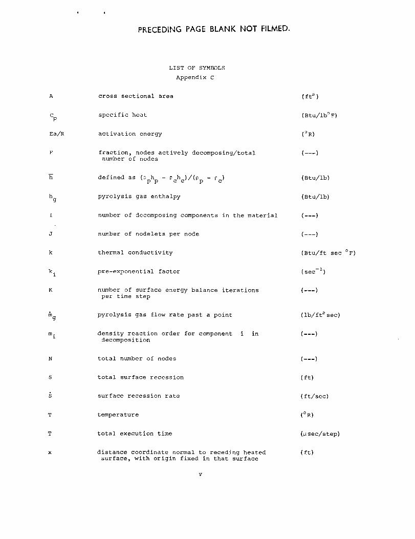
PRECEDING PAGE BLANK NOT FILMED.

LIST OF SYMBOLS

Appendix C

A

CP

Ea/R

cross sectional area

specific heat

activation energy

( ft _ )

(Btu/ib ° F)

(OR)

fractionj nodes actively decomposing/totalnumber of nodes

------)

hg

defined as (pphp - Pchc)/(pp - Cc )

pyrolysis gas enthalpy

number of decomposing components in the material

(Btu/ib)

(Btu/ib)

(---)

J

k

k.1

K

g

m.1

number of nodelets per node

thermal conductivity

pre-exponential factor

number of surface energy balance iterations

per time step

pyrolysis gas flow rate past a point

density reaction order for component i in

decomposition

(Btu/ft sec OF)

(sec -_ )

(---)

(ib/ft 2 sec)

---_)

total number of nodes ------)

S

T

total surface recession

surface recession rate

temperature

(ft)

(ft/sec)

(OR)

T total execution time (p sec/step)

X distance coordinate normal to receding heated

surface D with origin fixed in that surface

(ft)

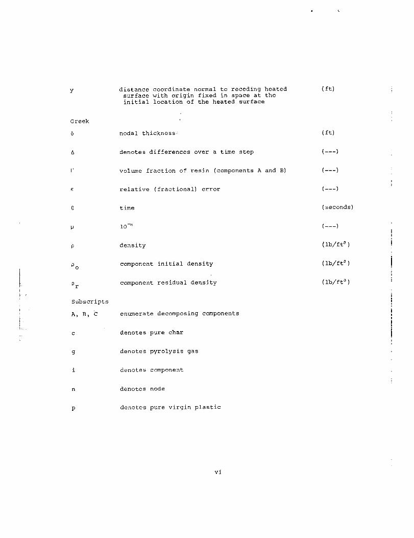
Y distance coordinate normal to receding heatedsurface with origin fixed in spaceat theinitial location of the heated surface

(ft)

Greek

6 nodal thickness_ (ft)

denotesdifferences over a time step

volume fraction of resin (components A and B)

relative (fractional) error

-----)

(---)

(---)

t ime (seconds)

c

F_

r

PO

Pr

Subscripts

A_ B_ C

C

g

i0-_

density

component initial density

component residual density

enumerate decomposing components

denotes pure char

denotes pyrolysis gas

----)

(ib/ft 8 )

(ib/ft 3 )

(ib/ft a )

denotes component

denotes node

denotes pure virgin plastic

v_

STUDYOFALTERNATIVETREATMENTSOFTHEDECOMPOSITIONKINETICSEQUATIONIN

THECHARRINGMATERIALABLATIONPROGRAM

C.] INTRODUCTION

This appendixreports the results of a numberof computational experi-mentsaimedat defining and eliminating causesof irregular or uneveninternalresponsesolutions occasionally producedby the AerothermCharring MaterialAblation Program(CMA). For economyreasons, the calculations described herewere limited to one material and a small numberof transient conditions.Hence, it has not beenpossible to extract manygeneral conclusions. However,the key problemshave beenfairly clearly identified, and in the process ofdoing so somesignificant improvementswere madein the programoperation.

Theappendix includes a numberof graphs which illustrate the effectof various computational techniques. To present all the interesting aspectsof the results would require an enormousmassof detail andmanypagesof com-puter output. Obviously a short memorandumcan only touch upona limited numberof aspects_ andhencethe report necessarily omits manydetails and takes ona descriptive nature.

C.2 SUMMARYOFCONCLUSIONS

The history of the instantaneous pyrolysis gas rate provides the mostsensitive index to the smoothnessof the internal responsesolution. Plots ofthis gas rate for slowly decomposingmaterials suchas the phenolics are smoothand regular regardless of the transient. The solutions to certain rather rareproblemshave irregular gas rates. Thesedo not affect the important overall

aspects of the solution and so generally even these rare irregular solutions

can be accepted. The boundary layer program (BLIMP) cannot accept irregular

solutions, however. Efforts to eliminate oscillations for this application

showed that:

i. Replacement of the explicit treatment of density in the decomposition

kinetic equation by exact integrated relations smoothed most solutions

and shortened computation time

2. Remaining unsmooth solutions could be smoothed by reductions in node

size

3. The number of nodelets per node has no importance for such problems.

Nodelets may be eliminated_ or greatly reduced in number_ with great

savings in computation time.

C-I

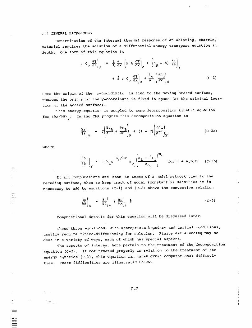
C. 3 GENERAL BACKGROUND

Determination of the internal thermal response of an ablating, charring

material requires the solution of a differential energy transport equation in

depth. One form of this equation is

P Cp_ x Aax a-_o y

s P Cp%-'_ e A _x ]e+

Here the origin of the x-coordinate is tied to the moving heated surface,

whereas the origin of the y-coordinate is fixed in space (at the original loca-

tion of the heated surface).

This energy equation is coupled to some decomposition kinetic equation

for (_p/_0)y. In the CMA program this decomposition equation is

_P (C-2a)+ I1- FI jy

z

b

F:

F

where

m.

( 1-Ei/RT Pi - Pri_Pi " - kie P°i _oi58 Y i

for i = A,B,C (C-2b)

If all computations are done in terms of a nodal network tied to the

receding surface, then to keep track of nodal (constant x) densities it is

necessary to add to equations (C-l) and (C-2) above the convective relation

x y 6

(C-3)

Computational details for this equation will be discussed later.

These three equations, with appropriate boundary and initial conditions,

usually require finite-differencing for solution. Finite differencing may be

done in a variety of ways, each of which has special aspects.

The aspects of interest here pertain to the treatment of the decompositionI

equation (C-2). If not treated properly in relation to the treatment of the

energy equation (C-l), this equation can cause great computational difficul-

ties. These difficulties are illustrated below.

I__

C-2

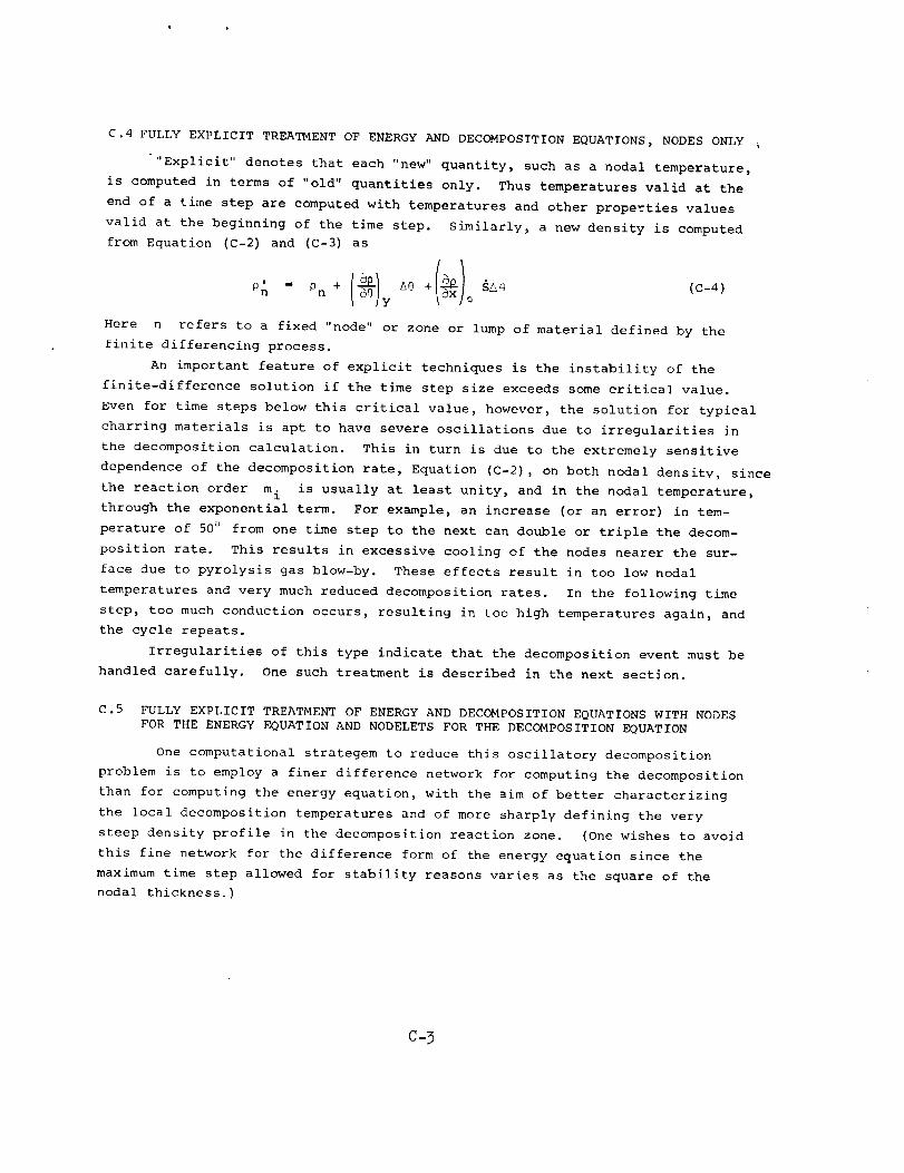
C.4 FULLY EXPLICIT TREATMENT OF ENERGY AND DECOMPOSITION EQUATIONS, NODES ONLY

"Explicit" denotes that each "new" quantity, such as a nodal temperature,

is computed in terms of "old" quantities only. Thus temperatures valid at the

end of a time step are computed with temperatures and other properties values

valid at the beginning of the time step. Similarly, a new density is computed

from Equation (C-2) and (C-3) as

On Pn + _ + SA_ (C-4)

y

Here n refers to a fixed "node" or zone or lump of material defined by the

finite differencing process.

An important feature of explicit techniques is the instability of the

finite-difference solution if the time step size exceeds some critical value.

Even for time steps below this critical value, however, the solution for typical

charring materials is apt to have severe oscillations due to irregularities in

the decomposition calculation. This in turn is due to the extremely sensitive

dependence of the decomposition rate, Equation (C-2), on both nodal density, since

the reaction order m i is usually at least unity, and in the nodal temperature,

through the exponential term. For example, an increase (or an error) in tem-

perature of 50 ° from one time step to the next can double or triple the decom-

position rate. This results in excessive cooling of the nodes nearer the sur-

face due to pyrolysis gas blow-by. These effects result in too low nodal

temperatures and very much reduced decomposition rates. In the following time

step, too much conduction occurs, resulting in too high temperatures again, and

the cycle repeats.

Irregularities of this type indicate that the decomposition event must be

handled carefully. One such treatment is described in the next section.

C.5 FULLY EXPLICIT TREATMENT OF ENERGY AND DECOMPOSITION EQUATIONS WITH NODES

FOR THE ENERGY EQUATION AND NODELETS FOR THE DECOMPOSITION EQUATION

One computational strategem to reduce this oscillatory decomposition

problem is to employ a finer difference network for computing the decomposition

than for computing the energy equation, with the aim of better characterizing

the local decomposition temperatures and of more sharply defining the very

steep density profile in the decomposition reaction zone. (One wishes to avoid

this fine network for the difference form of the energy equation since the

maximum time step allowed for stability reasons varies as the square of the

nodal thickness.)

c-3

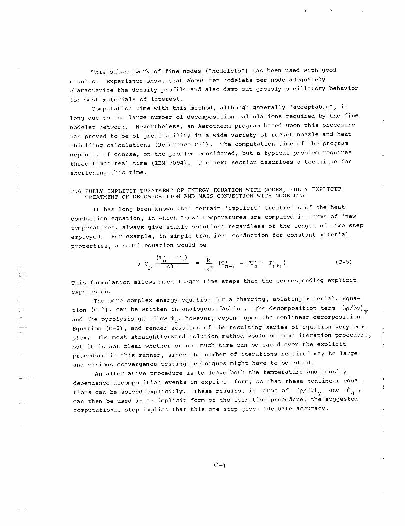
L

b

This sub-network of fine nodes ("nodelets") has been used with good

results. Experience shows that about ten nodelets per node adequately

characterize the density profile and also damp out grossly oscillatory behavior

for most materials of interest.

Computation time with this method, although generally "acceptable"_ is

long due to the large number'of decomposition calculations required by the fine

nodelet network. Nevertheless, an Aerotherm program based upon this procedure

has proved to be of great utility in a wide variety of rocket nozzle and heat

shielding calculations (Reference C-l). The computation time of the program

depends, of course, on the problem considered, but a typical problem requires

three times real time (IBM 7094). The next section describes a technique for

shortening this time.

C.6 FULLY IMPLICIT TREATMENT OF ENERGY EQUATION WITH NODES, FULLY EXPLICIT

TREATMENT OF DECOMPOSITION AND MASS CONVECTION WITH NODELETS

It has long been known that certain "implicit" treatments of the heat

conduction equation, in which "new" temperatures are computed in terms of "new"

temperatures, always give stable solutions regardless of the length of time step

employed. For example, in simple transient conduction for constant material

properties, a nodal equation would be

(Tn - Tn) = k ' + T' ) (C-5)

p Cp A9 6--_ (Tn-1 - 2Tn n+l

This formulation allows much longer time steps than the corresponding explicit

express ion.

The more complex energy equation for a charring, ablating material, Equa-

tion (c-l) , can be written in analogous fashion. The decomposition term _p/_0)y

and the pyrolysis gas flow _g, however, depend upon the nonlinear decomposition

Equation (C-2) , and render solution of the resulting series of equation very com-

plex. The most straightforward solution method would be some iteration procedure,

but it is not clear whether or not much time can be saved over the explicit

procedure in this manner, since the number of iterations required may be large

and various convergence testing techniques might have to be added.

An alternative procedure is to leave both the temperature and density

dependence decomposition events in explicit form, so that these nonlinear equa-

tions can be solved explicitly. These results, in terms of _p/_)y and mg ,

can then be used in an implicit form of the iteration procedure; the suggested

computational step implies that this one step gives adecuate accuracy.

c-4

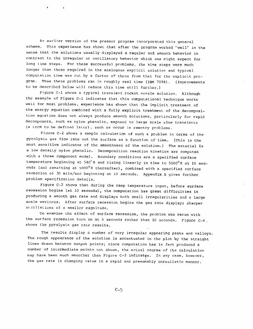
q I

An earlier version of the present program incorporated this general

scheme. This experience has shown that after the program worked "well" in the

sense that the solutions usually displayed a regular and smooth behavior in

contrast to the irregular or oscillatory behavior which one might expect for

long time steps. For these successful problems, the hime steps were much

longer than those required in the analogous explicit solution and typical

computation time was cut by a factor of three from that for the explicit pro-

gram. Thus these problems ran in roughly real time (IBM 7094). (Improvements

to be described below will reduce this time still further.)

Figure C-i shows a typical transient rocket nozzle solution. Although

the example of Figure C-i indicates that this computational technique works

well for most problems, experience has shown that the implicit treatment of

the energy equation combined with a fully explicit treatment of the decomposi-

tion equation does not always produce smooth solutions, particularly for rapid

decomposers, such as nylon phenolic, exposed to large scale slow transients

(a term to be defined later), such as occur _n reentry problems.

Figure C-2 shows a sample calculation of such a problem in terms of the

pyrolysis gas flow rate out the surface as a function of time. (This is the

most sensitive indicator of the smoothness of the solution.) The material is

a low density nylon phenolic. Decomposition reaction kinetics are computed

with a three component model. Boundary conditions are a specified surface

temperature beginning at 540°R and rising linearly in time to 5000°R at i0 sec-

onds (and remaining at 5000°R thereafter), combined with a specified surface

recession of 30 mils/sec beginning at i0 seconds. Appendix A gives further

problem specification details.

Figure C-2 shows that during the ramp temperature input, before surface

recession begins (at i0 seconds) _ the computation has great difficulties in

producing a smooth gas rate and displays both small irregularities and a large

scale waviness. After surface recession begins the gas rate displays sharper

o_zillations of a smaller magnitude.

To examine the effect of surface recession, the problem was rerun with

the surface recession turn on at 5 seconds rather than i0 seconds. Figure C-4 ,

shows the pyrolysis gas rate results.

The results display a number of very irregular appearing peaks and valleys.

The rough appearance of the solution is accentuated in the plot by the straight

lines drawn between output points; since computation has in fact produced a

number of intermediate points not shown, the actual course of the calculation

may have been much smoother than Figure C-3 indicat?s. In any case, however,

the gas rate is changing value in a rapid and presumably unrealistic manner.

c-5

Fortunately, the uneven behavior shown in Figures C-2 and C-3 is not usually

important. Abundant _omputational evidence, not to be reported here, indicates

that the ogerall aspects of the solution (total surface recession, total pyroly-

sis gas generation, surface temperature behavior, thermocouple temperature

behavior, char thickness, and isotherm penetration) are affected in only a very

minor degree by the irregularities.

There is at least one important case, however_ for which unevenness in

the gas rate would be unacceptable, and that is for the 6oupled boundary

laver solution (CABLE). Convergence of the boundarv laver computation will

De adversely affected bv too large jumps in the pyrolysis gas injection rate.

Therefore although uneven gas rate results are rare (being confined to a

limited number of materials exposed to a special kind of transient) and not

usually of importance, their influence on the boundary layer solution dictates

a closer study attempting to eliminate uneven behavior. Such a study has been

made and has resulted in significant improvements in computation procedures, as

described below.

C.7 TIME STEP LIMITATION BASED ON DENSITY CHANGE RATE

An early device employed to smooth out irregularities limited the time

step size according to an empirically determined limit on the density change

per time step of the fastest decomposing component in the material. This device

worked well in many problems, but for difficult cases it caused a sizable in-

crease in computation time. Thus there was a strong economic incentive to re-

move this "decomposition clamp".

C.S CHANGE IN TREATMENT OF DENSITY POTENTIAL IN DECOMPOSITION EQUATION FROM

FULLY EXPLICIT FINITE DIFFERENCE FORM TO EXACT INTEGRATED FORM

C.8.1 Introduction

Up to this point the decomposition relation, Equation (C-2), and the con-

vection relation, Equation (C-3), have been treated in the following explicit

manner:

i. Given "old" temperatures and "old" nodelet desnities for each compo-

nent i, "temporary" nodelet densities Are computed with the finite

difference convection relation (C-5).

2. These "temporary" densities are inserted into the decomposition

kinetic relation (C-4) and "new" nodelet densities compute_.

C-6

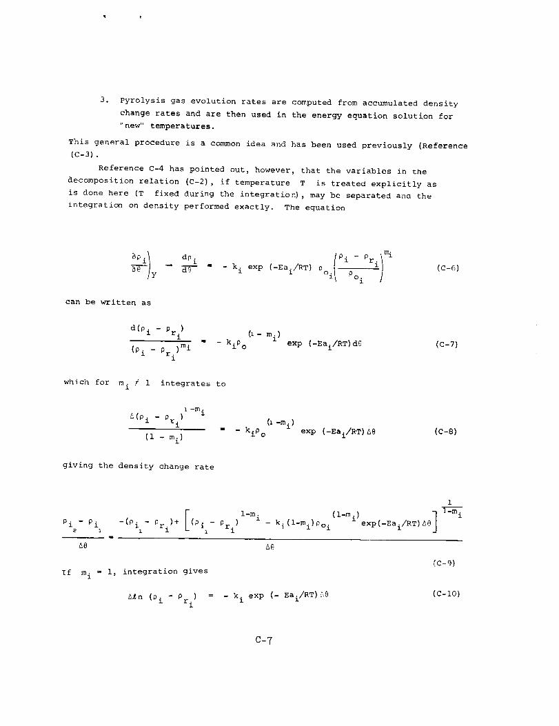
3. Pyrolysis gas evolution rates are computed from accumulated density

change rates and are then used in the energy equation solution for

"new" temperatures.

This general procedure is a common idea and has been used previously (Reference

(C-3) .

Reference C-4 has pointed out, however_ that the variables in the

decomposition relation (C-2), if temperature T is treated explicitly as

is done here (T fixed during the integration) _ may be separated ana the

integration on density performed exactly. The equation

Pi - Pr i_Pil dP i

B@ ]y d_ k i exp (-Eai/RT) po i P°i

(c-6)

can be written as

d(p i - pr)1

(Pi - Pr. )mil

(l- mi)

_ kip O exp (-Eai/RT) d8 (c-7)

which for m. / 1 integrates tol

i -m.

A(pi _ pr.) ll (_-mi)

, _ kiP O

(i - mi)

exp (-Eai/RT) A8(C-B)

giving the density change rate

l-m.Pi - Pi -(Pi - Pri)+ (Pi - Pr i) i _ ki(l_mi) Po iI I i

(l-m i)

exp (-Eai/RT) A@]

1

1

_8 Ae

if m i = I, integration gives

8_n (Pi - Pr. ) = - ki exp (- Eai/RT) 8@l

{c-9)

(C-10)

C-7

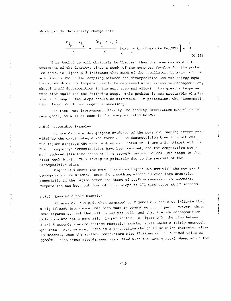
_ich yields the density change rate

Pi - Pi (Pi - Pr. )

- exp - k i _0 exp (- Eai/RT ) - 1

(C-11)

This technique will obviously be "better" than the previous explicit

treatment of the density, since a study of the computer r'esults for the prob-

lem shown in Figure C-3 indicates that much of the oscillatory behavior of the

solution is due to the coupling between the decomposition and the energy equa-

tions, which causes temperatures to be depressed after excessive decomposition,

shutting off decomposition in the next step and allowing too great a tempera-

ture rise again the the following step. This problem is now presumably elimin-

ated and longer time steps should be allowable. In particular_ the "decomposi-

t ion clamp" should no longer be necessary.

In fact, the improvement offer by the density integration procedure is

very great, as will be seen in the examples cited below.

C.8.2 Favorable Examples

Figure C-3 provides graphic evidence of the powerful damping effect pro-

_:ided by the exact integration forms of the decomposition kinetic equations.

The figure displays the same problem as treated in Figure C-2. Almost all the

"high frequency" irregularities have been removed, and the computation steps

much reduced (144 time steps at 11.9 seconds instead of 224 time steps in the

older technique). This saving is primarily due to the removal of the

decomposition clamp.

Figure C-5 shows the same problem as Figure C-4 but with the new exact

decomposition relations. Here the smoothing effect is even more dramatic,

especially in the region after the start of surface recession (5 seconds).

Computation has been cut from 645 time steps to 171 time steps at 12 seconds.

C.8.3 Less Favorable Examples

Figures C-3 and C-5_ when compared to Figures C-2 and C-4, indicate that

a significant improvement has been made in compu£ing technique. However, these

same figures suggest that all is not yet well, and that the new decomposition

relations are not a cure-a]]. In particular, in Figure C-3, the time between

3 and 5 seconds (before surface recession starts) still shows a fairly unsmooth

gas rate. Furthermore, there is a provocative change in solution character after

i0 seconds, when the surface temperature rise flattens out at a fixed value of

5000°R. B_th these a3pe_ts seem associate_ with the _ame 9_m_r_l phenomenon: the

C-8

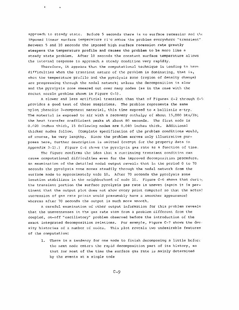
• t

approach to steady state. Before 5 seconds there is no surface recession and tl_

imposed linear surface temperature ri_e makes the problem everywhere "tuansient"_

Between 5 and i0 seconds the imposed high surface recession rate greatly

steepens the temperature profile and causes the problem to be more like a

steady state problem. After i0 seconds the constant surface temperature allows

the internal response to approach a steady condition very rapidly.

Therefore_ it appears that the computational technique is tending to }]ave

difficulties when the transient nature of the problem is dominating, that is,

when the temperature profile and the pyrolysis zone (region of density change)

are progressing through the nodal network; unless the decomposition is slow

and the pyrolysis zone smeared out over many nodes (as in the case with the

rocket nozzle problem shown in Figure c-l) .

A slower and less artificial transient than that of Figures C-2 through C-5

provides a good test of these suspicions. The problem represents the same

nyloq phenolic 3-component material, this time exposed to a ballistic entry.

The material is exposed to air with a recovery enthalpy of about 15,000 Btu/ib_

the heat transfer coefficient peaks at about 80 seconds. The first node is

0.020 inches thick_ 15 following nodes are 0.040 inches thick. Additional

thicker nodes follow. (Complete specification of the problem conditions would,

of course, be very lengthy. Since the problem serves only illustrative pur-

poses here, further description is omitted (except for the property data Jn

Appendix 3-1).) Figure C-6 shows the pyrolysis gas rate as a function of time.

The figure confirms the idea that a continuing transient condition can

cause computational difficulties even for the improved decomposition procedure.

An examination of the detailed nodal output reveals that in the period 0 to 70

seconds the pyrolysis zone moves steadily through the nodal network from the

surface node to approximately node i0. After 70 seconds the pyrolysis zone

location stabilizes in the neighborhood of node i0. Figure C-6 shows that durin_j

the transient portion the surface pyrolysis gas rate is uneven (again it is per-

tinent that the output plot does not show every point computed so that the actual

succession of gas rate points would presumably have a smoother appearance)

whereas after 70 seconds the output is much more smooth.

A careful examination of other output information for this problem reveals

that the unevennesses in the gas rate stem from a problem different from the

coupled, on-off "oscillatory" problem observed before the introduction of the

exact integrated decomposition relations. For example, Figure C-7 shows the den

sity histories of a number of nodes. This plot reveals two undesirable features

of the computation:

I. There is a tendency for one node to finish decomposing a little befor£_

the next node enters the rapid decomposition part of its history, so

that for most of the time the surface gas rate is mainly determined

by the events at a single node

c-9

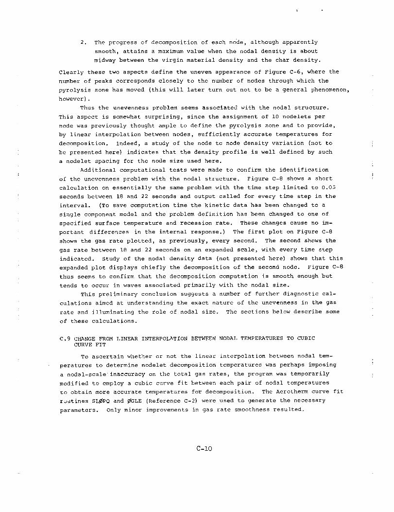
2. The progress of decomposition of each node, although apparently

smooth, attains a maximum value when the nodal density is about

midway between the virgin material density and the char density.

Clearly these two aspects define the uneven appearance of Figure C-6, where the

number of peaks corresponds closely to the number of nodes through which the

pyrolysis zone has moved (this will later turn out not to be a general phenomenon_

h oweve r ) .

Thus the unevenness problem seems associated with the nodal structure.

This aspect is somewhat surprising, since the assignment of i0 nodelets per

node was previously thought ample to define the pyrolysis zone and to provide r

by linear interpolation between nodes, sufficiently accurate temperatures for

decomposition. Indeed, a study of the node to node density variation (not to

be presented here) indicates that the density profile is well defined by such

a nodelet spacing for the node size used here.

Additional computational tests were made to confirm the identification

of the unevenness problem with the nodal structure. Figure C-8 shows a short

calculation on essentially the same problem with the time step limited to 0.05

seconds between 18 and 22 seconds and output called for every time step in the

interval. (To save computation time the kinetic data has been changed to a

single component model and the problem definition has been changed to one of

specified surface temperature and recession rate. These changes cause no im-

portant differences in the internal response.) The first plot on Figure C-8

shows the gas rate plotted, as previously, every second. The second shows the

gas rate between 18 and 22 seconds on an expanded scale, with every time step

indicated. Study of the nodal density data (not presented here) shows that this

expanded plot displays chiefly the decomposition of the second node. Figure C-8

thus seems to confirm that the decomposition computation is smooth enough but

tends to occur in waves associated primarily with the nodal size.

This preliminary conclusion suggests a number of further diagnostic cal-

culations aimed at understanding the exact nature of the unevenness in the gas

rate and illuminating the role of nodal size. The sections below describe some

of these calculations.

C.9 CHANGE FROM LINEAR INTERPOLATION BETWEEN NODAL TEMPERATURES TO CUBIC

CURVE FIT

To ascertain whether or not the linear interpolation between nodal tem-

peratures to determine nodelet decomposition temperatures was perhaps imposing

a nodal-scale inaccuracy on the total gas rates, the program was temporarily

modified to employ a cubic curve fit between each pair of nodal temperatures

to obtain more accurate temperatures for decomposition. The Aerotherm curve fit

rJ_tines SL_PQ and _GLE (Reference C-2) were used to generate the necessary

parameters. Only minor improvements in gas rate smoothness resulted.

C-10

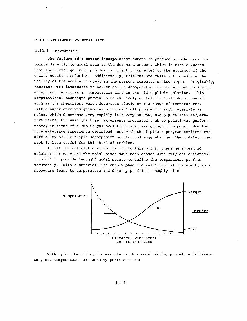
C.10 EXPERIMENTS ON NODAL SIZE

C.10.1 Introduction

The failure of a better interpolation scheme to produce smoother results

points directly to nodal size as the dominant aspect, which in turn suggests

that the uneven gas rate problem is directly connected to the accuracy of the

energy equation solution. Additionally, this failure calls into question the

utility of the nodelet concept in the present computation technique. Originally,

nodelets were introduced to better define dcomposition events without having to

accept any penalties in computation time in the old explicit solution. This

computational technique proved to be extremely useful for "mild decomposers"

such as the phenolics, which decompose slowly over a range of temperatures.

Little experience was gained with the explicit program on such materials as

nylon_ which decompose very rapidly in a very narrow, sharply defined tempera-

ture range, but even the brief experience indicated that computational perform-

mance, in terms of a smooth gas evolution rate, was going to be poor. Now the

more extensive experience described here with the implicit program confirms the

difficulty of the "rapid decomposer" problem and suggests that the nodelet con-

cept is less useful for this kind of problem.

In all the calculations reported up to this point_ there have been i0

nodelets per node and the nodal sizes have been chosen with only one criterion

in mind: to provide "enough" nodal points to define the temperature profile

accurately. With a material like carbon phenolic and a typical transient, this

procedure leads to temperature and density profiles roughly like:

Temperature

J i , , • , | , |

Distance, with nodal

centers indicated

- Virgin

Density

Char

With nylon phenolics, for example, such a nodal sizing procedure is likely

to yield temperatures and density profiles like:

C-ll

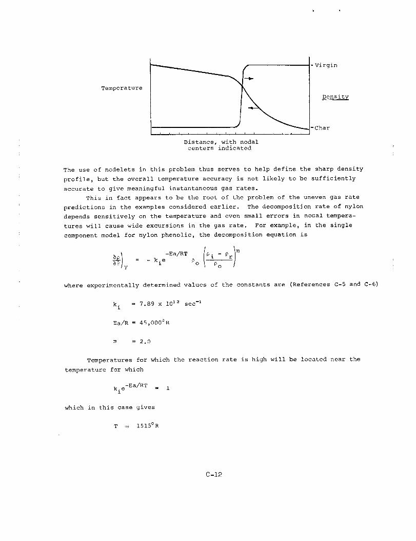
Temperature

f - Virgin

__ Chilns ity

Distance, with nodal

centers indicated

The use of nodelets in this problem thus serves to help define the sharp density

profile_ but the overall temperature accuracy is not likely to be sufficiently

accurate to give meaningful instantaneous gas rates.

This in fact appears to be the root of the problem of the uneven gas rate

predictions in the examples considered earlier. The decomposition rate of nylon

depends sensitively on the temperature and even small errors in noeal tempera-

tures will cause wide excursions in the gas rate. For example, in the single

component model for nylon phenolic, the decomposition equation is

= - k.e Poi PoY

where experimentally determined values of the constants are (References C-5 and C-6)

k.1

= 7.89 x I012 sec -i

Ea/R = 45,000aR

m =2.0

Temperatures for which the reaction rate is high will be located near the

temperature for which

k.e -Ea/RT = 1l

which in this case gives

T _ 1515°R

C-12

! t

Therefore, when the decomposition rate is of importance it will be roughly

proportional to

4_000

_P iso0 (i+_) e-3O/(i+ _) e-aO (i-e) e-a0ea0¢

d

Thus a relative error in temperature of e causes a relative error in decom-

position rate of e 3°_. For T = 1500°R, errors of 5°R, 10°R, 20°R, and 30°R

give the following errors in decomposition rate

_ ea0 c

5 1/300 1.105

10 1/150 1.221

20 2/150 1.492

30 3/150 1.822

Hence even a 5 ° error in a nodal temperature will cause a 10% error in the gas

rate, when the temperature is high enough for the decomposition to be important.

A 5 ° error represents about 1/2% of the total nodal temperature rise in typical

problems.

The main drift of these observations then is that the accuracy of the

temperature solution seems directly involved with the uneven gas rate problem.

The following section adduces further evidence to this effect.

C.I0.2 Experiments with Smaller Node Sizes

If accuracy of the temperature solution underlies the gas rate problem,

the only solution to the trouble consists of smaller node sizes. Figure C-9

shows the same problem as illustrated earlier in Figure C-6 (aside from the minor

changes to a single component decomposition and a specified surface temperature

and recession rate problem rather than a surface thermochemistry problem),

but with 0.02 inch nodes instead of the former 0.04 inch nodes. The improve-

ment is striking, the amplitude of the gas rate "waves" being reduced by about

half.

Thus it seems that nodal size is the dcminant parameter, and that perhaps

the number of nodelets per node is more or less irrelevant for this particular

problem. To check this aspect, the problem of Figure C-9 was recompu£ed once

again with 0.008 inch nodes, but with only two nodelets per node. This yields

the same nodelet size as for the problem of Figure C-6. The results, shown in

Figure C-10, may be compared to the earlier results for the same problem shown

in Figures C-6 and C-9. Again the "wave amplitude" has been much reduced.

C-15

Figure C-10 has a conspicuousdip in the gas rate at 25 seconds. Ithappensthat the specified surface temperatureboundarycondition for thisproblemhas a markeddecreasein slope at 25 seconds; to check if perhaps thiscausedthe gas rate dip the problemwasrerun with a rampinput for surfacetemperatureand recession rate. Figure C-II showsthe results and proves thatirregular behavior is characteristic of the computational systemrather thanthe specific boundarycondition.

As a final test of the effect of smaller nodes on the smoothness of the

solution, the ramp input problem of Figure C-II was rerun with a new nodal

size distribution. The first node was 0.008 inch, and the next seven nodes

were 0.016 inches thick. These nodes were followed by _ number of nodes of

0.004 inches thickness, half as large as the nodes of the problems illustrated

in Figures C-10 and C-II. Figure C-12 shows the results of this last computa-

tion. As expected, during the time the pyrolysis zone is progressing through

the thick nodes (in this problem 0 to 30 seconds) the gas rate is very

irregular. As soon as the pyrolysis zone passes into the thin nodes, the gas

rate smooths out almost completely, except for one small wave at 38 seconds.

The computations illustrated in Figures C-6, C-9, C-10, C-ll, and C-12

thus indicate that the choice of nodal size and number of nodelets per node

determines the smoothness of the pyrolysis gas rate. It would, of course, be

desirable to have quantitative criteria for selecting these quantities, but

the overall complexity of this problem seems to dictate a trial and error

procedure. To facilitate the selection of these quantities, Appendix C-2 pro-

vides some useful estimates of program execution time as a,function of the

number of nodes and nodelets.

C.II CONCLUSIONS

The early versions of the Aerotherm Charring Material Ablation Program,

which treated the decomposition kinetic equations explicitly in both density

and temperature and which used an implicit formula for the energy equation in

depth, produce excellent results for slow decomposers such as phenolics

regardless of the type of transient involved. Fast decomposers such as nylon

cause irregularities in the solution values of quantities of interest,

especially in the rate of pyrolysis gas generation, for those particular

transient problems in which the pyrolysis zone is passing rapidly through the

nodal network (which is tied to the receding heated surface).

Usually these irregularities cause no problems since experience shows

that they do not affect the important overall aspects of the solution, such

as total surface recession and char thickness, for example. However_ since

it is expected that irregularities in the pyrolysis gas rate will cause

convergence difficulties in the coupled boundary layer program (BLIMP), the

present study included attempts to eliminate irregular or wavy gas rate

predictions.

C-14

An early computational strategem lumped the rapid decomposition effect

into one of the available three decomposing constituents and then applied a

time step limit to the overall solution to prevent the decomposition rate

(density change rate) of this component from exceeding some empirically deter-

mined amount. This semi-rational time step limit was quite effective, but

turned out to be rather costly for nylon, which for many transients requires very

short time steps for a smooth solution.

A better smoothing procedure abandons the explicit treatment of density

in the decomposition relations in favor of exact integrated relations for the

density dependence. The implicit-density nature of these relations exerts a

powerful smoothing effect on the solution, and allows removal of the time step

clamp on decomposition rates with a consequent saving in the number of solution

steps. Although the integrated decomposition relations are about twice as slow

to compute as the simpler explicit relations, the saving in time steps in diffi-

cult to handle problems was observed to be a factor of four to five in the num-

ber of time steps. Since the computation time is mainly devoted to decomposi-

tion, net computation time has been cut by about a factor of two.

Despite the strong smoothing effect of the implicit density relations,

certain particularly unfavorable combinations of materials and boundary conditions

can still cause markedly uneven gas rate predictions. The roots of this behavior

could not be definitely identified due to the complexity of the internal response

solution. Computational experiments demonstrated, however, that nodal size is

the key parameter affecting the smoothness of the solution, which points to the

overall accuracy of the energy solution as the key aspect. Smaller node sizes

resulted in much smoother solutions and no doubt remains that entirely smooth

solutions can be obtained with "sufficiently" small nodes. With small nodes

the nodelet structure becomes of minor importance, and the number of nodelets

can be cut down to the minimum (within the present program logic) of two without

harm to the solution. Thus, the net computation time is in general not increased

by the smaller node size.

It would, of course, be desirable to have a quantitative criterion for

selecting nodal and nodelet sizes, but the overall complexity of the problem

appears to preclude a successful analysis and to demand an empirical approach.

To date, computational experience has not been sufficient to define any general

rules giving good nodal sizing.

C-15

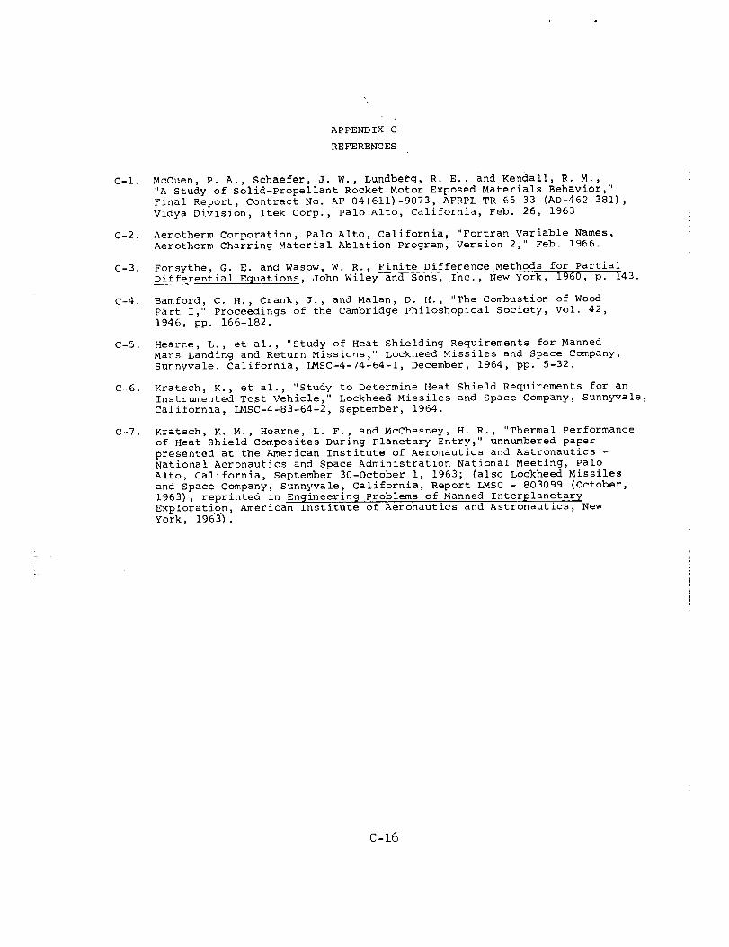
APPENDIX C

REFERENCES

C--l.

C--2.

C--3.

C--4.

C-5.

C-6.

C-7.

McCuen, P. A., Schaefer, J. W. j Lundbe_g_ R. E._ and Kendall_ R. M.,

"A Study of Solid-Propellant Rocket Motor Exposed Materials Behavior,"

Final Report, Contract No. AF 04(611)-9073, AFRPL-TR-65-33 (AD-462 381),

Vidya Division, Itek Corp., palo Alto, california, Feb. 26, 1963

Aerotherm Corporation, Palo Alto, California, "Fortran Variable Names_

Aerotherm Charring Material Ablation Program, Version 2," Feb. 1966.

Forsythe, G. E. and Wasow, W. R., Finite Difference Methods for Partial

Differential Equations, John Wiley and Sons, Inc., New York, 1960, p. 143.

Bamford, C. H., Crank, J., and Malan, D. H., "The Combustion of Wood

Part I," Proceedings of the Cambridge Philoshopical society, Vol. 42,

1946, pp. 166-182.

Hearne, L., et al., "Study of Heat Shielding Requirements for Manned

Mars Landing and Return Missions," Lockheed Missiles and Space Company,

Sunnyvale, California, LMSC-4-74-64-I, December, 1964, pp. 5-32.

Kratsch, K., et al., "Study to Determine Heat Shield Requirements for an

Instrumented Test Vehicle," Lockheed Missiles and Space Company, Sunnyvale,

California, LMSC-4-83-64-2, September, 1964.

Kratsch, K. M., Hearne, L. F., and McChesney, H. R., "Thermal Performance

of Heat shield Composites During Planetary Entry," unnumbered paper

presented at the American Institute of Aeronautics and Astronautics -

National Aeronautics and Space Administration National Meeting, Palo

Alto, California, September 30-October i, 1963; (also Lockheed Missiles

and Space Company, Sunnyvale, California, Report LMSC - 803099 (October,

1963), reprinted in Engineerin 9 Problems of Manned Interplanetary

Exploration, American Institute of Aeronautics and Astronautics, New

York, 1963).

C-16

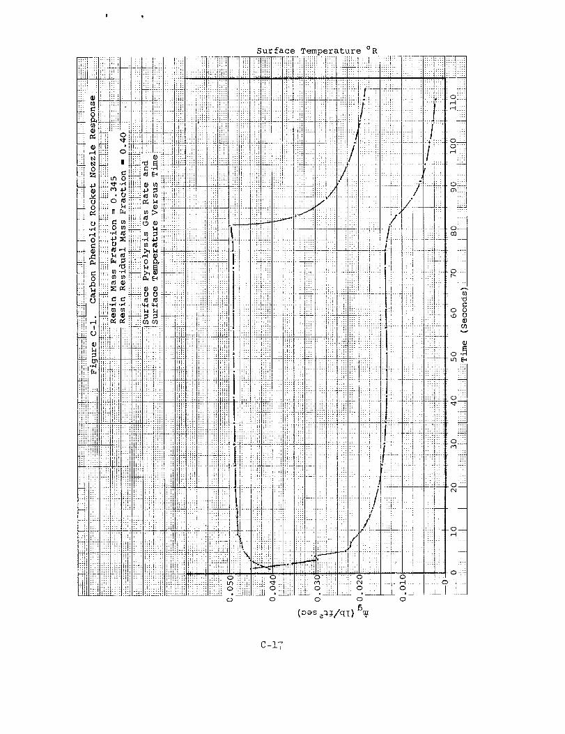
) t

o

Surface Temperature °R

o

{:jo o

6o

co o

03

o-_

C-!7

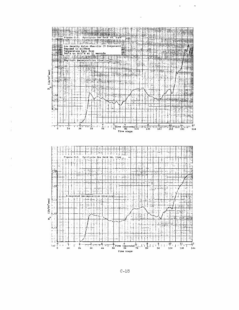
_'_ {: _ _ _ :_._ :_]_,_-_-._ ET_:_=_< :_ :_ i i .= :!!_=P:% _=_ m_ _7_ii_'_ ,_iT_i:_3÷" _i_:={

:_ Figure C-2. Pyrolysis Gas Rate vs. Tim_'--_e-_ :_.__n_i_÷_ _! t_ _=_-_=:_

:1!1£:Y'< _ .... 4 } . :!L: t--- [:_:F_.:_=I::=_::-[> .%L.. kI[:''- [[i:[ : L.,., [[ NI::[;: "i" _: _ _] i-[ ". [!:?%:t:i_

IF.

I-

0 i 3 4 _ 7_i_ime 6 7 1 2I-_---t_-T-ZT-F-T---I -_ 4--.4 _4--%.-. I -: 4i .4-,-i-,4

0 14 39 56 86 105 125 143 162 -- 191 ' 224

Time steps

_O.OS

C-18

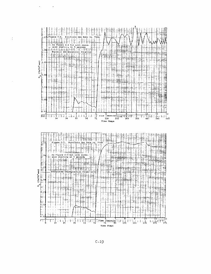
0.0-

0.07

i ±] i

0 1 2 3 4 5 6 7 8 2

Time Steps

C-!9

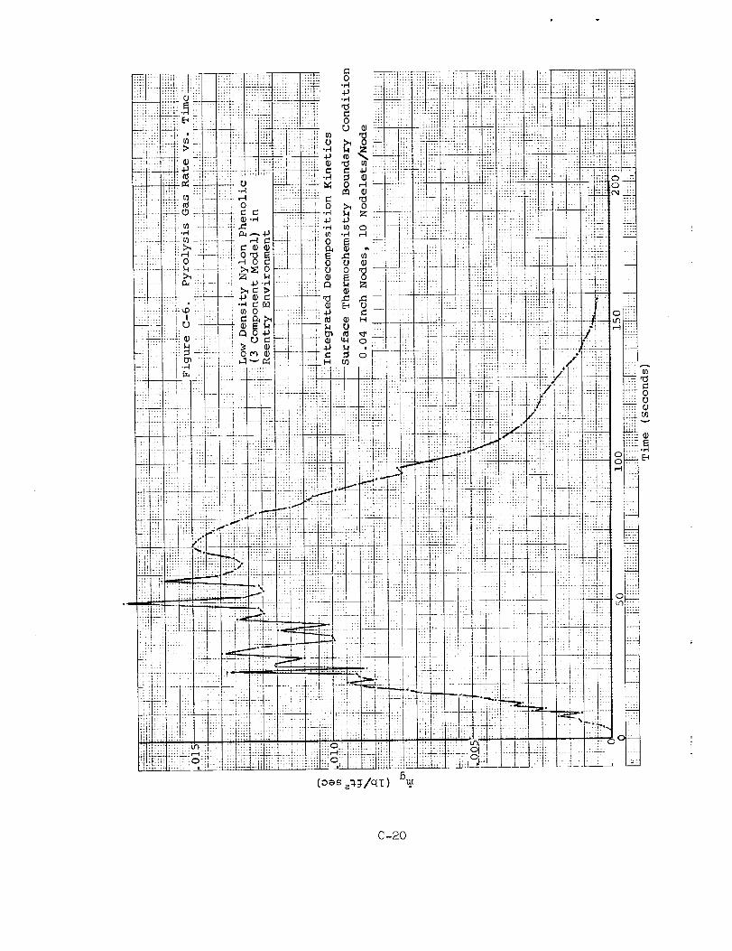
(_es _%_/qI) Bu_

idi:!l

!E>

2

°i1,TTT o

_._

t:;t

0 "'"_..ik_ :x

rxt

_........_

C-20

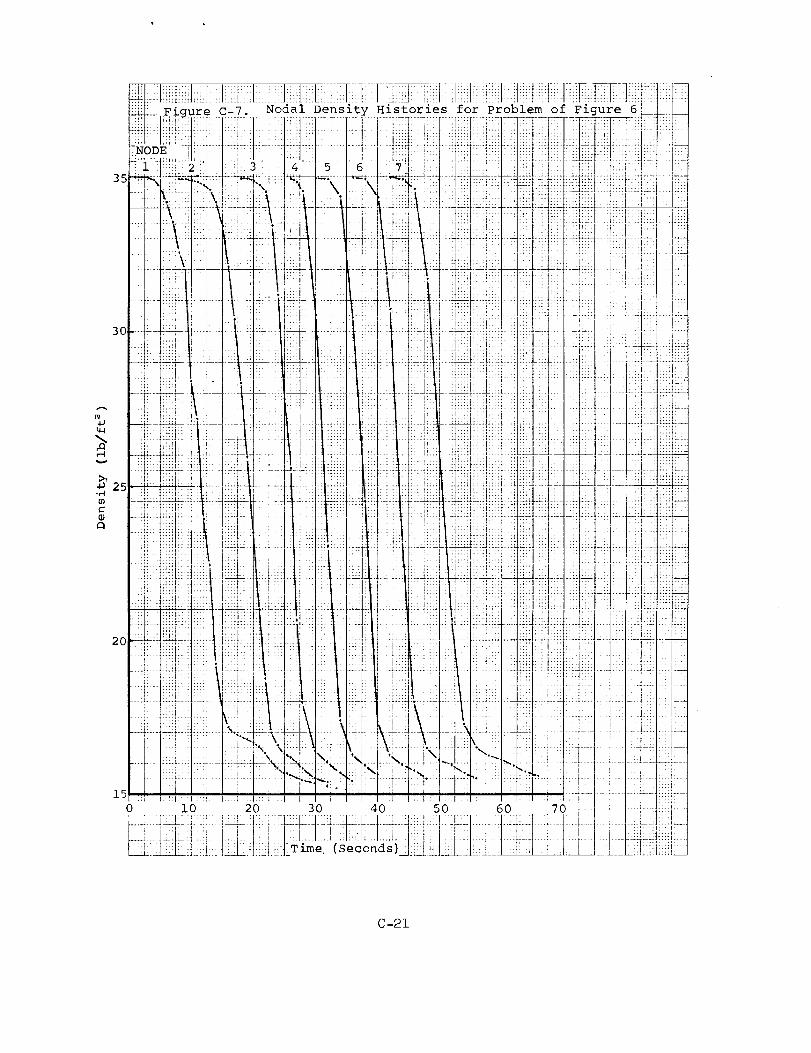
35

30;

Figure C-7. Nodal Density Histories for Problem of Figure 6 __i_ _

_;NODE = [

i :ikL : [

:t:" Y::i-i• ....... -°

....[:: ....... IL \

I ° . I

..... i:'):

::i]: i

_:ii:::i:_iilL!I: : ::::1: _ !

.... {: lib]

2=. ][: :::I:::'"

:!1:s'

!)_i"t

:iLl : :

i5 ; <:i-:'11

o lO

-:i:::211:_i:::::::I: :q

- : '::::

: - =[..::

J:_ ._::'_S_

_ Z 2M

% :: ;:

;| . ._±-:z

:': U

L; _::2:2.'=2-

:l::.'

:;;:::

i!. ii:!::

:L ; =: iL

:!i : iFi

22- . ::=i' "--'

ii:iii

-k:

5Oi: IF v

'::tl;;; :.z:

?}!i!! i!ii

iiii!iiii_i!:ili[ii=i:;il

11121:;i::;...... i: .il

]::;L;;; .;:

:!:t:i:: ::!

2;Ji2±iii!i[ilq:i:i

);12[Z22iit;::}1:;' ::::

:i:i!iii :i!

!iiilii2iiill

" :P-:; ::'1

i:::]122±:];::I.S: ;:

:LJ=2i_2

i::! : :!i:::I:: i!

!:ili:i; !;:::tr:

22_: _:i

LII :;L

"..,.. i

t :

60i i"

25:2__:

:;:: ::::H:::;

";:: :; ':If:i:

::.=::]:I:i:2

-, ::: [;.:,

_--L::L:Ii

::::2:1::

:I_C!I!::iii:::LJi:_ i:ii{iii:::-Z:I

::_:_................::::l:i::1::b. I"

iii2[iLi.i..ii:i!!1212_.

_i_ikll[iii[i_ _!:[i_ii12[2::!ii::.Z2.21..__

:! : i:: I :!I

:l t : : ]: :i

;;;.I...; :: : ±z_± : :!ZZ_

:=:_c4

.................i:2:

i;i!i '?!:......21..:2

......i',iZl::i21 i;i!:i

ii::l:::: :q!

,2:1.........._iiLi: _2__

.__..:.... _....... _:_:=:_-.-_-:t t

.... } i I : ::: !!i-!:-i

70 _= : t _:__:+_ . .:.... [..:...... !._:..±L:

C -21

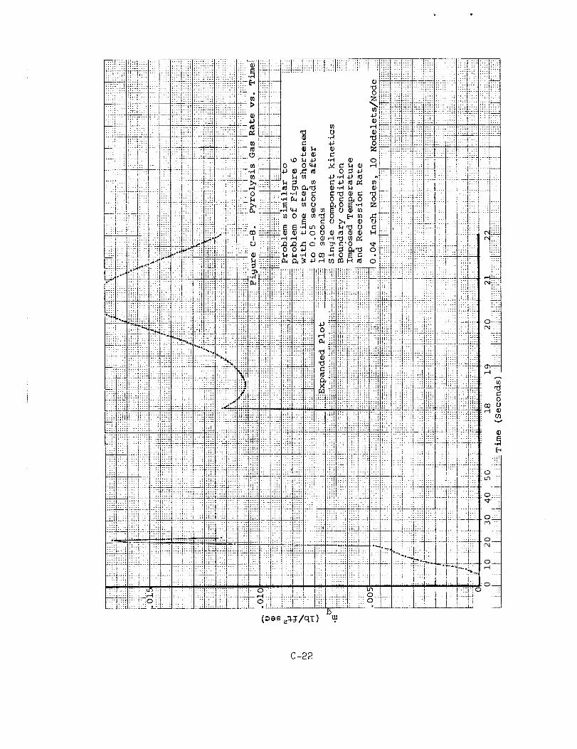
:Zili!

_i!iiiiilii!:

_ili_i!?ii:::_

i!iiii:il

+:---

i!i!:i

!!iilii:!

F-IiF.:

::L ::¶

....Ii

ilJ{iii:::!!L!:

....I,..

ii:_ili-L

, i ,,

) ::[

i!!:Hi: !iiil

ii_i_iiiiiii

_i::ii:il:!!i

:_:!ii_i__:_;!il

if!U!: !!_

i!iili!il:!ii

i:i:iii!i!i:i

,iiLiiLJ_

: l:,:,!li!I:: IU

:ii:_

ii_,i•

2_<['

1!::

:::!:_;!;!_"• ::f:":': 0._.!:_:::::::

:::' :: 0 _._JL ] -_ ® _ c:::: ;:::

:_:::: ::_ :' _[ ]0 0 0_ _M C _ • ,--I]_ : :::::

:: ...... ._ _:_ h _ -_'_ -_ _ _1:::, ::: :

: : :.::]i _ _-,-I _ _ 0 0 _ D._O OL

: :!::: ::: : " ::::: : :: :: :i:::: : :::: _:: : : : ::::

::::i:::l:)q::::::::::t:::::::!I::,::!::::iii:t ::::: l::::i _::1:::1: i if :,]:ii/ iit-_i :: t:J:i. J:::,

::U:: I:::F o ; ::: : ::::.:!::: :. m

]5

(_ _,::/g:)

::: ::::: :! :: !:: .......

:-:-L

!:!!:::_li_:]:{::l:::it::::::Ii:,i_I= i:iiiil :i:_::

2_.2

::2 ;2i_[2:l:Li:.... ::__q! ................. :oL

! ...... .o._:

:: <!°½

C-22

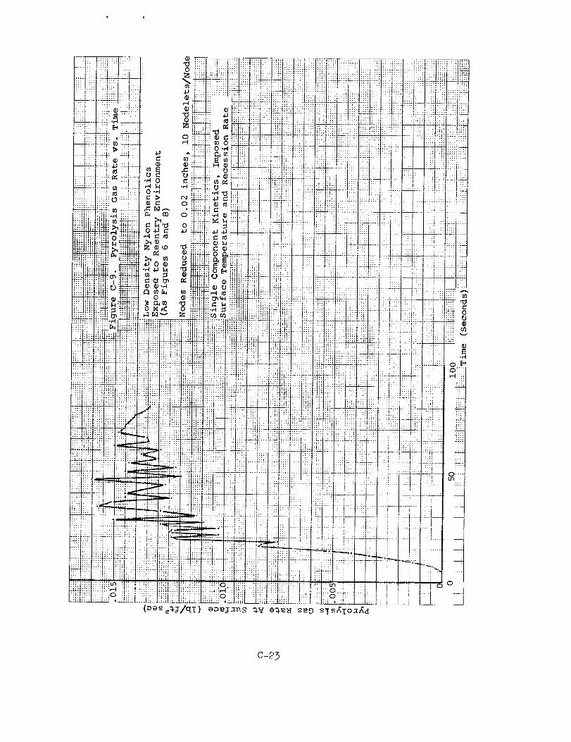
C-25

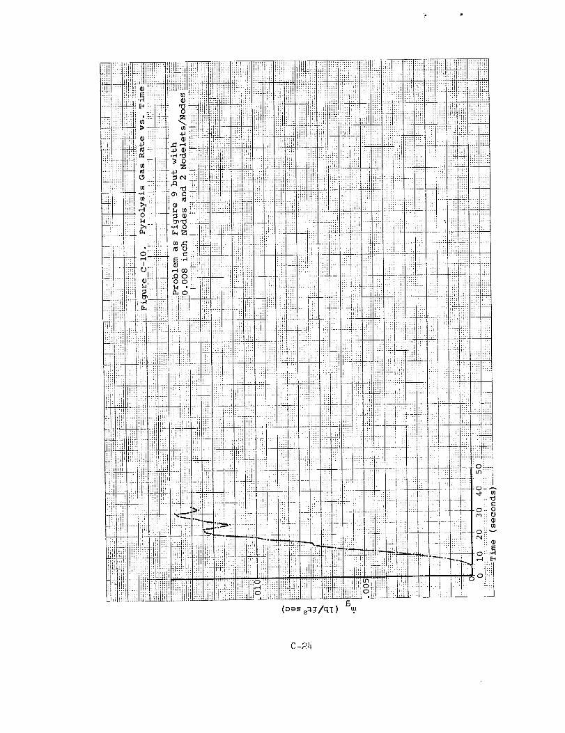
iiii;sl!!i!_iii! ::::!!!:i_::'_:_:_ .... :i: ,i:@i :.iii i;i ....._ ::!:,!:

........ _ii: :ii L!!!_I .........k:_._

ii!;!i::L: :!!ilili:iH!;l i! !i ;:,_;_ i ! ,_:}i i

i',_ ::'_ ::_:h!!: !:i,Y.i :i!i:: :!

:::";:: ...... ::i!{i :::

L_:_i_:-_ ::_:4::_ ::: 1.:;: ::_:; :. :; :i:il i:il

:ii t::: ..... :;.'. ::. i:4[::':: :::

....... ' .: £'4 _ _._:__ ::::!;:_::.:-

:_:,!...._-i_:ii_:i,t._:i ........: !i! _:: i!i l{i!i _:.,

...... L_H ::: : .......:!i{

Y:i :_: : ........... r4LL :LL +_!:_ :- ---_ .... _ .... 4:_--- ._-:

ili ::_:_ii:::: Y. 2 _:!!_i iili :" :_ _:_........... -2: .:..i: --:-:

!:i :!::!?_:lii 11:17 _::':_:_:::,.....• I

..... ....... ,r: ......!:! ii!' !'. ........ _:_i

B

_i!iiii...............

i:!i_ ;!YJ!i :

::.:[::: I :1: !:::|: ::

.... :: liH "

i: ....

i::_ :-!!!i:ii!t_+ :iiiL2

/:;: 2:H;::: :ii:l:iL

:y. ....

:i: :4i:_ _:L_I iii$ii4

....Z :i::!_::_::i_44:Ii:.::: iA:_iiii!:::}::1 ii1:i?

.:ii:_i .... '*.....iiili!{i

÷::i::2: _4siaS44: : : 1: . ::;;;

:......... :i:_,_: !:!}i'+-

: ....... i,li: : u-,)::-:

.... _ " ; : U)

- '-' U1-'- -

-_ c:_x 1: !: m1

i i :!i o

C-2_

_!iili_i !!iii_il_,_:_,: _

i!::t::!i .... _:' !!i?t_;:! I-:.: ..... t:;L':!

::7!1:;_

i:I xC:: : _i:ii.... : :1:::

fill" "H'; ' :

<'_: i i!i!{ :! i'_:_

!!i! :" ............. .L±5 ,I-,_

iI! ........_22 ::' :.i....

_il i_ _, ........

..... i

........ !:-i-! 0:_ 8!-Ii:.5 : m ....

i;ti;_ '

0-25

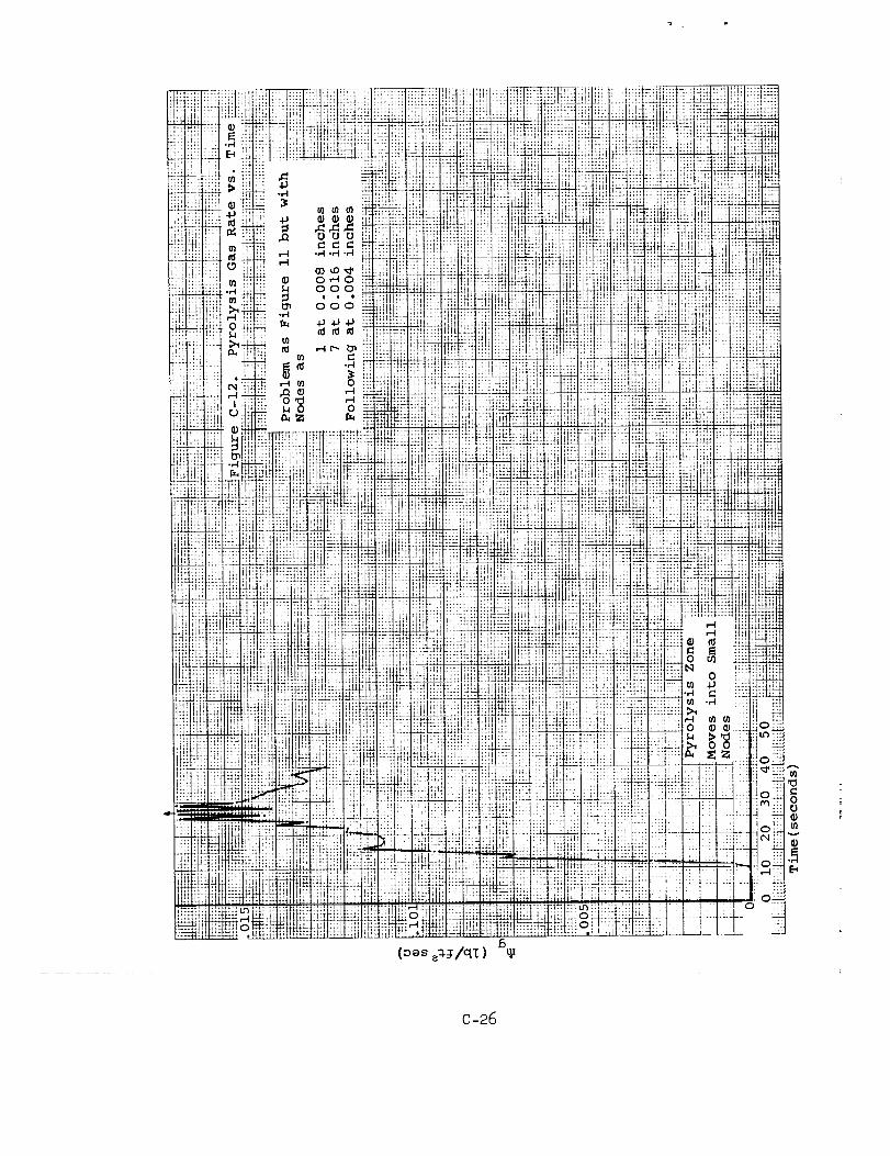
i :ii

i]i iii;4; :::

;Ii

1i:

2! i:!) :_!

_g!i !:ii :rr

!ii ;;_

1:i2:,

_A

2; :d

:ii!

_5

:i

k:,

.g

v

C-26

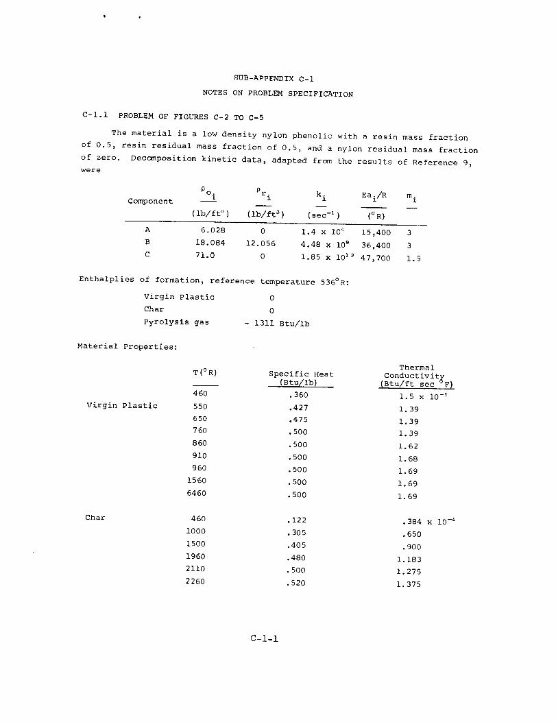
SUB-ADPENDIX C-I

NOTES ON PROBLEM SPECIFICATION

C-I.I PROBLEM OF FIGURES C-2 TO C-5

The material is a low density nylon phenolic with a resin mass fraction

of 0.5, resin residual mass fraction of 0.5, and a nylon residual mass fraction

of zero. Decomposition kinetic data, adapted from the results of Reference 9,

were

Pro k. Eai/R mP°i l l 1

Component -- __ __

(ib/ft 3 ) (ib/ft 3) (sec-1) (o R)

A 6.028 0 1.4 x 104 15,400 3

B 18.084 12.056 4.48 x 109 36,400 3

C 71.0 0 1.85 x 1013 47,700 1.5

Enthalplies of formation, reference temperature 536°R:

Virgin Plastic 0

Char 0

Pyrolysis gas - 1311 Btu/ib

Material Properties:

Virgin Plastic

Thermal

T(°R) Specific Heat Conductivit_

(Btu/Ib) (Btu/ft sec F)

460 .360 1.5 x i0 -E

550 .427 1.39

650 .475 1.39

760 .500 1.39

860 .500 1.62

910 .500 1.68

960 .500 1.69

1560 .500 1.69

6460 .500 1.69

Char 460 .122 .384 x lO -4

i000 .305 .650

1500 .405 .900

1960 .480 1.183

2110 .500 1.275

2260 .520 1.375

C-l-i

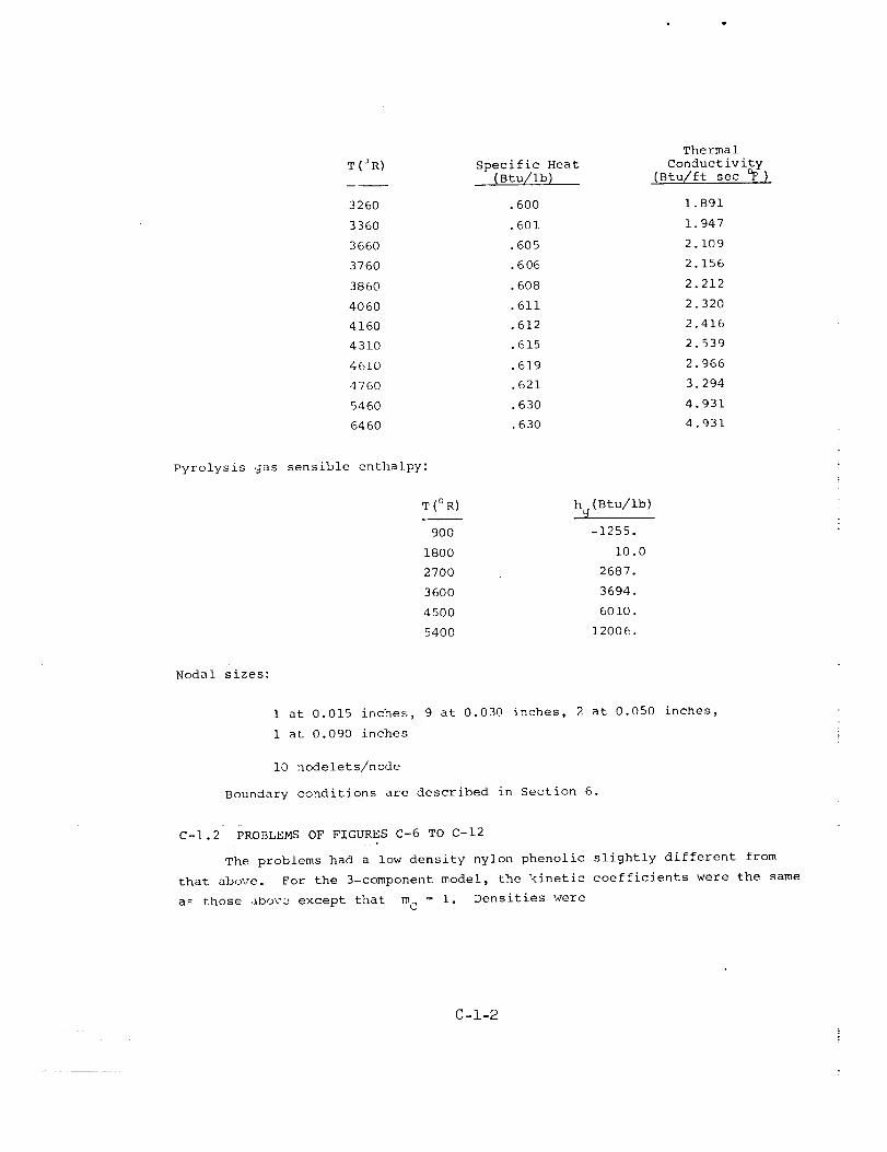
T (_ R)

3260

3360

3660

3760

3860

4060

4160

4310

4610

4760

5460

6460

Specific Heat

(Btu/ib)

6OO

601

6O5

606

6O8

611

612

615

619

621

630

630

Thermal

Conductivity

(Btu/ft see _ )

1.891

1.947

2.109

2.156

2.212

2.320

2.416

2.539

2.966

3.294

4.931

4.931

Pyrolysis gas sensible enthalpy:

T(°R) h (Btu/ib)

900 -1255.

1800 I0.0

2700 2687.

3600 3694.

4500 6010.

5400 12006.

Nodal sizes:

1 at 0.015 inches, 9 at 0.030 inches, 2 at 0.050 inches,

1 at 0.090 inches

i0 nodelets/node

Boundary conditions are described in Section 6.

C-].2 PROBLEMS OF FIGURES C-6 TO C-12

The problems had a low density nylon phenolic slightly different from

that above. For the 3-component model, the kinetic coefficients were the same

a_ those ;iDove except tha£ m C = i. Densities were

C-I-2

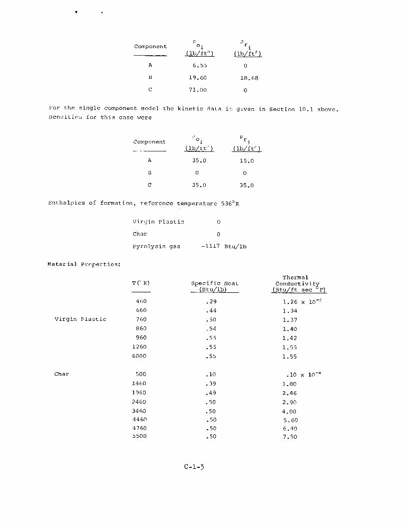
0Component oi Pri

,( ib/ft a ) J_

A 6.55 0

B 19.60 18.68

C 71.00 0

For the single component model the kinetic data is given in Section i0.i above.

Densities for this case were

WO • Pr,Component ] ]

(ib/ft _') (ib/ft _)

A 35.0 15.0

B 0 0

C 35.0 35.0

Enthalpies of formation, reference temperature 536°R

Virgin Plastic 0

Char 0

Pyrolysis gas -1117 Btu/ib

Material P copert ies:

Virgin Plastic

Thermal

T(_R) Specific Heat Conductivit[(Btu/ib) (Btu/ft see F)

460 .29 1.26 x i0 -c

660 .44 1.34

760 .50 i. 37

860 .54 1.40

960 .55 1.42

1260 .55 1.55

6000 .55 1.55

Char 500 .i0 .I0

1460 .39 1.80

1960 .49 2.46

2460 .50 2.90

3460 .50 4.00

4460 .50 5.60

4760 .50 6.40

5500 .50 7.50

x 10 -4

C-i-3

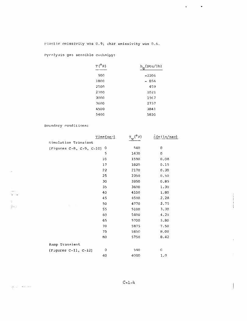
L

!:

l'lastic emissivity was 0.9; char emissivity was 0.6.

Py]-o]ysis gas sensible enthalpy:

T(°R) h (Btu/ib)

900 -2206

1800 - 854

2500 459

2700 1021

3000 1967

3600 2757

4500 3841

5400 5850

Boundary conditions:

Time(

Simulation Transient

(Figures C-8, C-9, C-J0) 0

5

10

17

22

25

30

35

4O

45

5O

i5

6O

65

7O

75

80

Ramp Transient

(Figures C-If, C-12) 0

4O

se_:l Tw(° R) S (mils/sec)

540

1430

1590

1820

2170

2350

2850

3600

4100

45O0

4770

5100

5400

5700

5875

5850

5750

540

4000

0

0

0.08

0.15

0.30

0.50

0.85

i. 30

i. 80

2.28

2.75

3 30

4 25

5 80

7 50

8 O0

8 42

0

1.0

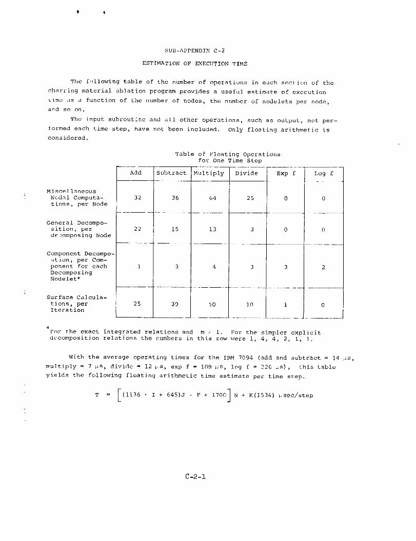
SUB-APPENDIXC-2

ESTIMATIONOFEXECUTIONTIME

The f_llowing table of the numberof operations in each sec[ion of thecharring material ablation program provides a useful estimate of execution

time as a function of the number of nodes_ the number of nodelets per node,

a_d so on.

The input subroutine and all other operations, such as output, not per-

formed each time step, have not been included. Only floating arithmetic is

considered.

Miscellaneous

Nodal Computa-

tions, per Node

General Decompo-

sition, per

decomposing Node

Component Decompo-

stion, per Com-

ponent for each

Decomposing

Nodelet*

Surface Calcula-

tionsj per

Iteration

Table of Floating Operations

for One Time Step

Add

32

22

25

Subtract

36

15

Multiply

64

13

Divide

25

39 5O ]0

Exp f

1

Log f

For the exact integrated relations and m _" I. For the simpler explicit

decompositJon relations the numbers in this row were i, 4, 4, 2, i, i.

with the average operating times for the IBM 7094 (add and subtract = 14 _s,

multiply = 7 _s, divide = 12 _s, exp f = 188 _is, log f = 226 _s) , this table

yields the following floating arithmetic time estimate per time step.

T = [(1136 I + 645)J • F + 1700] N + K(1534) usec/step

C-2-1

mD

where

T

I

j =

F =

N =

K =

= execulion time for a single time step (_sec)

= number of decomposing components in the material

nltmber of nodelets per node

fraction of nodes decomposing

total ntunber of nodes

n_nber of iterations in _urFace e:_ergy balance

To estimate tntal execution time, T may be multiplied by the total num-

bec o[ _ ime steps, a number approximately determim<l _y the user in the choice

_,f the maximum time step allo_.,.ed. F should be In ,_verage value for the frac-

tion of nodes actively decomposing during the pl.-ob[em (usually between 1/3 and

I/2). A study of numerous problems reveals that K a_er_ges very close to 3.

The resulting total time must be multiplied by a factor to account for

"alministr,.tJve" arithmetic such as DO loop indc_<inq. Experience with this

program on the 7094 suggests a factor between 1.4 and I. ,.

A,[d_ti_na] machine time will be consumed by s,lput and lo_dJng operations,

,)v_)r]ay or special tal_e handling (i[ necessary), and output ope_atlons, the

details of which are peculiar to individual computing facilities.

C-2 -2

4

APPENDIX D

TRANSFORMATION OF THE IN-DEPTH ENERGY EQUATION

!

E

i

ii

E

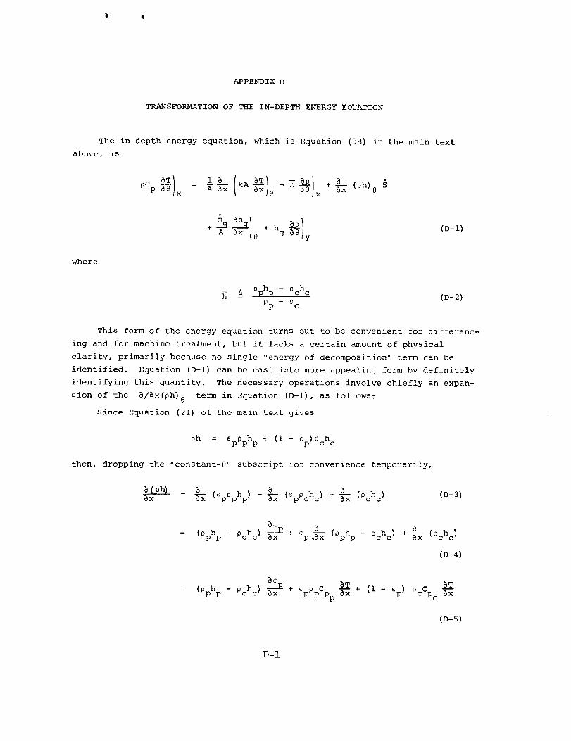
APPENDIX D

TRANSFORMATION OF THE IN-DEPTH ENERGY EQUATION

The in-depth energy equation, which is Equation (38) in the main text

above, is

A5xl_ kA 8-x_aT - h x + _-_ (ph) 8

A _x ]8 g Y

(D-l)

where

pphp - Pchc

Pp - Pc

(D-2)

This form of the energy equation turns out to be convenient for differenc-

ing and for machine treatment, but it lacks a certain amount of physical

clarity, primarily because no single "energy of decomposition" term can be

identified. Equation (D-l) can be cast into more appealing form by definitely

identifying this quantity. The necessary operations involve chiefly an expan-

sion of the _/_x(ph) 8 term in Equation (D-l), as follows:

Since Equation (21) of the main text gives

ph = eppphp + (i - ¢p) 0ch c

then, dropping the "constant-8" subscript for convenience temporarily,

_x = _ (_.ppphp)-_ (_pPchc) + _ (Pehc) (D-3)

_ Pchc ) +(pphp- Pchc ) _ + Cp._-_ (pphp Tx (Pchc)

(D-4)

_c _T

(p_p- 0c_c)_+ c p c _T _cP P PP _-_ + (I - ¢p) u Pc

(D-5)

D-I

But by the defining Equation (28) of the main text

+

OCp = CpppCpp (i- ep) PcCpc

(D-6)

so that

= (pphp- Pchc ) 8x I0 pCp _-_x 8@

(D-7)

Now, however, we have by Equation (20) of the main text that

p = eppp + (i - ep) Pc(D-8)

so that

= Pp - Pc %x }8e(D-9)

or

8x ]8 Pp- Pc

Substituting this into Equation (D-7) gives finally

(D-10)

where h is defined by Equation (D-2) above.

Now substitution of Equation (D-II] into the original energy Equation (D-I)

gives

) IpCp_ x = N_ _P + SpCp _TIkh-_x +h S 5x 8 x- _-{)0

A 8x ]8 + hg _ Y(D-12)

D-2

P •

But the conservation of mass Equation (15) of the main text gives

(D-13)

Putting this into the h coefficient above und collecting terms we obtain

the desired final relation

A 8x _ O (hg Y 4 Si,Cp _x 0 + A 8;< ]j (D-14)

This equation may be viewed as a "conservation of sensible energy" equa-

tion at constant x, and thus has a close relation with the usual form of

energy equations in applications including chemical changes. The second term

on the right hand side represents the "creation of sensible energy" due to

pyrolysis.

NASA-Langley, 1968 -- 33 CR-I061 D-3