N

eleconferencing: Cost Optimization of

Satellite and Ground Systems for

Continuing Professional Education

and Medical Services

(NASA-CR-133359) TELECONFERENCING: COST N73-2910OPTIMIZATION OF SATELLITE AND GROUNDSYSTEMS FOR CONTINUING PROGRESSIONALEDUCATION AND MEDICAL SERVICES (Stanford UnclasUniv.) p HC CSCL 17B G3/07 11394

May 1972

Stanford University, Stanford, California

The research in this document has been supportedby the National Aeronautics and Space Administration

RADIOSEIERIE LABORATORV

STRflFORD UlIUERSITV STIRIFORD, CALIFORI9REPRODUCED BY

NATIONAL TECHNICALINFORMATION SERVICE

U. S. DEPARTMENT OF COMMERCESPRINGFIELD, VA. 22161

This research was sponsored by NASA Grant NGR-05-020-541

Principal Investigators were:

Donald Dunn - Engineering Economic Systems

Bruce Lusignan - Electrical Engineering

Edwin Parker - Communications

Student Research Assistants were:

Chapter II Ra3y Panko, Ron Braeutigam

Chapter III Kinji Ono

Chapter IV Daniel Allnn, Carl Mitchell

Chapter V James Potter

Chapter VI & VII Carl Mitchell

Teleconferencing: Cost Optimization of Satellite

and

Ground Systems for Continuing Professional Education

and

Medical Services

Institute for Public Policy AnalysisStanford University, Stanford, California

The research in this document has been supported

by

National Aeronautics and Space Administration

May, 1972

Table of Contents

I. Introduction and Summary .... ........ . . . I- 1

. Demand for TeleconferencingA. Introduction .. .... . . . . . . . .. . . . . . . II- 1B. Teleconferencing Markets and Services

1. Service Categories . ... .. . . . . . . . . . . II- 42. Continuing Professional Education .. . . . . . . . II- 5a. Problems with Traditional Systems . . . . . . II- 7b. Behavioral Considerations. .. . . . . . .... .II- 10c. The Establishment of a National Information

Network .. . . . . . . . .. II- 12d. Probable Architecture of Future Networks . . . II- 14e. The Economies of Integration . . . . . . . . . II- 16f. The Desirability of Teleconferencing . .... II- 17g. A Scenario of Professional Education . . . . . II- 183. Remote Medical Services . . . . . . . . . . . . . II- 23a. Medical Applications of Teleconferencing . . . II- 23b. Classes of Users .. .... . . . . . . . . . . II- 26c. Rural and Ghetto Services . . . ......... . . II- 29d. Regional Networks . . . . .... . . . . . .II- 31e. The Need for Teleconferencing .. . . . . . . . II- 33

4. Business Teleconferencing . . . . ......... . . . II- 33C. Demography . . . . . . . . . . . . . . . . . II- 35

1. Demand Assement . . ........ . . . . . . . . II- 36a. Medical Services.. * * * . II- 36b. Continuing Professional Education . . . . . II- 40

2. System Design . .. . . . . . ................ . II- 47a. People Based Systems . . . .............. II- 48b. Industry Based Systems . . . . . . . II- 56c. Summary . . .. . . ................. II- 66

3. Case Studies in Demography . ....... .. II- 67a. Electronic Manufacturers in the San Francisco

Bay Area . . .. . . . ................. . . II- 68b. San Jose Detailed Analysis . . . ......... . . II- 72c. Doctors in the Salt Lake City Metropolitan Area II- 76d. Doctors, Lawyers, & Teachers in Denver

Metropolitan Area ............. II- 79e. Doctors in the State of Colorado . . . . . . . II- 84f. The Rocky Mountain Area . . ........... II- 87g. Summary .. ................. II- 89

D. A Methodology for Demand Assessment . . . ....... . . II- 901. Characteristics and Assumptions of the Study . . . II- 902. Estimating Potential Demand . . . . . . . . . . II- 923. Converting Potential Demand to Actual Demand .. . II- 954. Plausibility of System to User .. . . . . . . . II- 965. Tariffs (Pricing) .. . . . . . . . . . . . . II- 986. Acceptance of Inovation .. . . . . . . . . . . . II- 1037. Putting It All Together--Demand . . . . . . . . II- 107

i

Table of Contents (Continued)

8. Example Calculation: Determinations of Price andSubstitute Elasticities of Demand ....... II-109

9. Elasticity Calculations. ......... . . 11-11310. Limitations of the Methodology. ... ..... II-117

E. References . .. ............... . . ..11-127

III. Cost Analysis of Satellite Ground StationsA. Introduction . .. . . . . . . . . . . . . . . III- 1B. Antenna Gain . ........... . . . . . .... . III- 2C. Receiving System Noise Temperature .. . . .. . . . . III- 2D. G/T versus Antenna Diameter . ............ III- 3E. Cost versus Antenna Diameter . ... ....... . . III- 4F. Cost versus Pre-amplifier Noise Temperature . .... III- 9G. Cost versus G/T. .......... .. . . . . . . III- 9H. Cost Savings for Mass Production . ......... III- 12I. EIRP versus G/T ............... . . . . III- 12J. Cost versus Transmitter Power .... ...... . III- 19K. Installation Cost .......... .... . . . III- 19L. Maintenance and Operation Costs . . . .. . ..... III- 20M. Site and Maintenance Costs . .... ........ III- 27N. Conclusions ........ .. . . . . . .... III- 300. References .. ..... . ...... . . ......... . . ... III- 31

IV. Space Segment CostsA. Introduction. . ...... . ............... IV- 1B. Methodology . ........ * . .. .......... IV- 2

1. Three Candidate Satellites . ......... . . IV- 22. Supply and Demand Functions . .. ..... . . .. IV- 53. Economies of Scale .. ........ . . . . . . ... IV- 54. Present Value Comparisons . ...... . . . . . . IV- 85. Annual Cost . ........ . . . . . . . . . . IV- 10

C. Results and Conclusions ......... . . . . . . . . . IV- 10D. References .. . . . . . . . ..................... . IV- 20

V. Minimum Cost Satellite Teleconferencing NetworkA. Introduction ... . . . . ..... .. . . . . . . . . . . V- 1

1. Statement of the Problem. . ...... . . . . . . . V- 12. Review of the Literature. . .... . . . . . . . V- 9

B. Analytical Framework . . . . . . . . . . . . . . . V- 101. Cost Equation .. . . . ......... . . . . . V- 102. Noise Budget . . . . .. . . ........ . •. . . V- 123. Cost Data . . . . . . .. .. .. . . . . . V- 134. State Equations .... .. ... .. . . . . . . . V- 175. Signal-Quality Constraints. . . . . . . . . . . . V- 236. Intermodulation Distortion . . . . . . . . . . . V- 267. Modulation Procedures . . . . . . . .......... . V- 31

a. Multiple Access . . . . . .. .. . . . . . . V- 31b. Demand Assignment . ... . . . . . . . . ... V- 33c. Video Link. . ............ . . . . V- 35

ii

V. (cont.)

C. Fixed Satellite Parameters: Optimization of theGround Segment. . . . . . . . . . . . . . . . . . . . . V- 381. Identical Slave Stations . . . . . . . . . . . . . V- 382. Classes of Slave Stations . . . . . . . . . . . . .. V- 45

D. Optimization of Both Ground and Space Segments . . . . . V- 471. Analysis . .. . . . . . . . . . . . . . . . .. V- 472. Summary of Results . . . . . . . . . . . . . V- 51

E. Symmetrical Satellite Teleconferencing Networks. . ... . V- 601. Two-Way Video. . . . . . . . . . . ...... . . . V- 602. One-Way Video Plus Symmetrical Voice . . . . . . . . V- 633. Hybrid Satellite/Terrestrial Networks. . . . . . . . V- 64

F. Conclusion.. . . . . . . .. . ...... ... . . V- 691. Summary of Results . . . . . . . . . . . . . . . . . V- 692. Suggestions for Future Research. . . . . . . . . . . V- 713. Possible Implications .. . . . . ..... . . . . . . V- 73

G. References . . . . . . . . . .. ....... ..... . V- 74VI. Electronic Communications Equipment Costs For Terrestrial

SystemsA. Introduction . ... ..... . . . . . . . . . . . . . VI- 1B. Local Distribution Systems Equipment . . . .... . . . VI- 2

1. Cable .. ...................... VI- 22. ITFS ........................ VI- 4

C. Point-to-Point Systems Equipment . . . . ........... . . VI- 81. Cable. . . . . . . . . . VI- 82. ITFS . .. . . . ....................... VI- 83. Microwave . . .. .............. . . . . VI- 10

D. Summary . . . . . . ........................ VI- 12E. References . . . .. . . . . . . ..................... . VI- 13

VII. Least-Cost Comparison of Alternative TeleconferencingA. Introduction . . . . . . . . . . VI....................... VII- 1B. Long-Distance Transmission Subsystems . . . . . . . . . VII- 1

1. Long-Distance Transmission Subsystemsa. The Terrestrial Microwave Network. . .... . . VII- 1b. The Satellite/Earth Station Network . . . .... VII- 4

2. Cost Summariesa. Satellite. . .. . . . . . .................. . VII- 5b. Terrestrial Microwave. . . . . ............... VII- 9

C. Long-Distance Subsystem Comparison . . . . ........... . VII- 10D. Local Distribution Subsystems . . ........ . . . . . . VII- 13

1. Community Demographic Model . . . . . ........... . VII- 152. Cost Equation for Configuration A & B. . ....... . . VII- 173. Cost Comparisons . . ..... . . . . . . . . . . VII- 18

E. Summary. . . . . . . . . . . ....................... . VII- 21F. References . . ....... . . .... .. . . ............ . VII- 22

APPENDICESAPPENDIX A: Computer Assisted Instruction (CAI) ...... . . A-IAPPENDIX B: Supply: Discounted Launch Streams . ....... . .. B-1APPENDIX C: Demand: Discounted Sold Capacity . .. ...... . C-1

iii

APPENDICES (Cont.)

APPENDIX D: Comparative Evaluation of the Medium SatelliteCase . . . . . . . . . . . . . . . . . . . . . . . D-1

APPENDIX E: The Number of Cities In The Rocky Mountain RegionIn Three Size Categories. . ............ . E-1

iv

LIST OF ILLUSTRATIONS

Figure Page

II-1. Electronics Manufacturing Company Having 20 or MoreEngineering Employees. . ..... .... . . . . II- 69

11-2. Distribution of Engineering Employees by Size of.Firm in Bay Area . .. ... ... ........ .II- 71

11-3. Doctors in San Jose Area - Part I. . . . . . . . . II- 73

11-4. Doctors in San Jose Area - Part II . ... . .. .II- 74

11-5. The Salt Lake City Metropolitan Area . ... . . . II- 77

II-6. The Denver Metropolitan Area. . ...... . . . . II- 80

11-7. Doctors In The State of Colorado Against thePopulation. ..... ............... . . II- 85

II-8. The Adoption Curve . ....... ........ II-105

11-9. Adoption Curve for Example Analysis (from Rogers,Diffusion of Innovations) . ........... II-111

Figure

III-1. G/T vs. Antenna Diameter . ... ......... III- 4

111-2. Cost vs. Antenna Diameter. . ........... . III- 6

111-3. Cost vs. Antenna Diameter. . ........... . III- 7

111-4. Cost vs. System Noise Temperature. ..... ... . III- 9

III-5. Cost vs. System Noise Temperature. . .. . . . III- 10

111-6. Antenna Diameter vs. G/T Which Gives a MinimumCost Combination of Antenna and Pre-Amp . ... . III- 12

111-7. Cost vs. Antenna Diameter. . ... ......... . . III- 13

111-8. Cost vs. System Noise Temperature . .. .... .III- 14

111-9. Cost of Antenna and Pre-Amplifier vs. G/T. . .. . III- 15

III-10. EIRP vs. G/T For Given C/T ........... . . III- 17

III-11. Power Amplifier Cost vs. Output Power. ... .. .. III- 19

111-12. Power Amplifier Cost vs. Output Power. .. .... III- 20

111-13. Cost of Power Supply, Water Supply and Miscellaneous III- 21

v

ILLUSTRATIONS (cont.)

Figure Page

111-14. Ground Station Cost vs. G/T. ... ... . . . . . III- 22

111-15. M & O Cost of Antenna. . ... ............ . III- 24

111-16. O & M Cost of Pre-Amplifier. . ........... . III- 25

111-17. 0 & M Cost of Power Amplifier . ...... . . . . III- 26

III-18. Building Cost of Ground Station . ...... ... . III- 28

111-19. Site Cost of Ground Station . ........... III- 29

Figure

IV-1. Supply and Demand Functions. . ... ......... . III- 6

IV-2. Costs For Constant Demand. ... ........... III- 14

IV-3. Cost For Mixed Demand. .. ... ........... III- 15

IV-4. Cost For Linear Demand . .. ............ III- 16

Figure

V-1. Satellite Teleconferencing Networks. . ...... . V- 6

V-2. (C/T) im vs. Backoff V- 29

V-3. Video Multiplexer Configurations .......... . V- 36

V-4. Fixed Satellite Parameters; N Identical Slave Stations V- 44

V-5. Variable Satellite Parameters; N Identical SlaveStations. ... ...... . . . . . . . . . . . . . V- 52

V-6.0-6.6. Variable Satellite Parameters. ...... .. . . . . V- 54

V-6.7-6.12. FDMA vs. TDMA. . ....... . .... . . . . . V- 55

V-6.13-6.16. FDMA vs. TDMA . . .. .. .. .. . .. .. . . . V- 56

V-6.19-6.24. Miscellaneous Cost Comparison (FDMA) ..... . . . . V- 59

vi

ILLUSTRATIONS (cont.)

Figure V (cont.) Page

V-7.0-7.4. Two-Way T.V. . .. ... ............. . V- 62

V-8. One-Way T.V. Plus Symmetrical Voice. ........ . . V- 65

V-9. The Star and the Mesh. . . .. ......... . . V- 67

Figure

VI-1. Microwave Mid-Path Clearance vs. Path Length, for K=1and f=2.6 GHz . . . . . . . . . .. . . . . . . . . VI- 9

Figure

VII-1. A Rectangular Teleconferencing Region ContainingN Uniformly Distributed Cities. . ........ . VII- 3

VII-2. Terrestrial Microwave and Satellite System Costs vs.N, the Number of Cities in the Networas (C=4) VII-11

VII-3. Terrestrial Microwave and Satellite System Costs vs.N, the Number of Cities in the Networks (C=12) VII-12

VII-4. A Demographic Model of a Community . ... .... . VII-16

APPENDICES

APPENDIX D.D-1. Timing of Launches to Meet Linear Demand Growth D-2.

D-2. Present Value of Investment vs. Discount Rate,Annual Cost per Watt vs. Discount Rate . . . . . .. D-5.

vii

LIST OF TABLES

Table Page

II-1. Major Professional Occupational Groups. .. . . . . . II- 3

11-2. Trends in Hospitals .. ....... . . . . . . . . II- 37

11-3. Inpatient Health Facilities . ... .. .. . . . . . . II- 38

11-4. Occupations of Employed Persons 18 yrs. Old & Older(May 1969) .. . . . . . . . ................... . II- 41

11-5. Demand for Classroom Teachers in Elementary & Secon-dary Schools, to 1979 .. ......... . . . . . . . II- 42

11-6. Demand for Instructional Staff In Higher Education II- 43

11-7. Growth Rates In Selected Professions. . . ........ . II- 44

11-8. Highest Degree of Scientists, 1968. . ... ..... II- 46

11-9. Scientists, By Field & State, 1968 . ........ . II- 49

II-10. Physicians, By Type of Practice (1967) ... ... . II- 52

II-11. Fields of Employment of Registered Nurses (1967). . II- 53

11-12. Scientists In Private Industry by Industry, 1967. . II- 54

11-13. Government Employment, 1969 .. ... .. ....... . . 11II- 57

11-14. Financial Institutions, 1969. ....... ... . . . II- 58

11-15. Number of Public School Systems by Size of System,1966-67. . . . . . . . . ..................... . .. II- 59

11-16. Number of Institutions of Higher Education, Fall 1969 II- 60

11-17. Employment in Hospitals, 1966 .... ... . .. . . II- 61

11-18. Full-Time Personnel In Nursing & Personal Care Facili-ties: April-July, 1968 .. .... . . ........ . . II- 62

1I-19. Reporting Units Under Social Security (1968). ..... . II- 64

11-20. Bed Size of Hospitals, 1968 . . .. . . . . . . II- 65

11-21. Doctors in the Salt Lake City Metropolitan Area . . II- 78

II-22. Doctors and Lawyers in the Denver Metropolitan Area . II- 81

1I-23. Teachers in the Denver Metropolitan Area. .... .... 1II- 83

viii

TABLES (cont.)

Table II (cont.) Page

11-24. Portion of Places in Colorado Having No Doctors bySize of Place. ..... ... ........ .... . . II- 86

11-25. Rocky Mountain Region Number of Places, by Size. . II- 88

11-26. Occupational Classifications (Bureau of Census) . . . II- 91

11-27. Geographical Area Classifications . . . . . .. . . . II- 93

11-28. Price-Market Share Schedule. .......... . .. . . . II-100

11-29. Market Share Factor for Non-uniform Tariff. ... .. . II-100

I-30. Example Values for A.. and G. M . . . . . . . . . II-110

II-31. Demand Calculations and Results ..... . . . ...... II-112

Table

III-1. Antenna Alternatives. .... . . . . ...... . . III- 5

111-2. Pre-Amp. Alternatives . . ............ . III- 8

111-3. Power Amplifier Alternatives. . .... ... . ... III- 18

Table

IV-1. Satellite Attributes and Costs. . ..... . . . . . III- 3

IV-2. Discounted Capacity: Supply and Demand. . ...... . III- 11

IV-3. Present Value of Investment; and Annual Cost per Watt III- 13

Table

V-1. Antenna Cost/Performance Data .. ........ . V- 16

V-2. Ground Segment Cost/Performance Data. ... .... . . V- 18

V-3. Cost/Performance of Master-Station Multiplexer. . . V- 22

V-4. The Relative Efficiency of.D.A. Satellite Circuits. . V- 69

ix

TABLES (cont.)

Table Page

VII-1. (N) for Representative Values of N. . ... . ..... VII- 4

VII-2. Satellite System Cost Parameters with C -

$15,000 and c=4. . . . . . . . . . . . . . . . VII- 7

VII-3. Satellite System Cost Parameters with C =$30,000 and c=4 . . . . . . . . . . . . . . . . VII- 7

VII-4. Satellite System Cost Parameters with C =

$50,000 and c=4. .. . . . . . . ............ . VII- 7

VII-5. Satellite System Cost Parameters with C =

$15,000 and c=12 . . . . . . . . . . . . . . . . . VII- 8

VII-6. Satellite System Cost Parameters with C =

$30,000 and c=12 .. . . . . . . . . . . . . . . VII- 8

VII-7. Satellite System Cost Parameters with C =

$50,000 and c=12 . . . .. . . . .. . . . . . . VII- 8

TABLES IN APPENDICES

APPENDIX A: Computer Assisted Instruction (CAI) . ...... A-1

APPENDIX B: Supply: Discounted Launch Streams . ...... B-1

APPENDIX C: Demand: Discounted Sold Capacity. . ....... C-1

APPENDIX D: Comparative Evaluation of the Medium Satellite

Case . . . . . . . . . . . . . . . . . . . . . D-1

APPENDIX E: The Number of Cities in the Rocky Mountain RegionIn Three Size Categories . ........ . . E-1

x

Chapter I

Introducation and Summary

The study just completed developed a set of analytical capabilities

that are needed to assess the role satellite communications technology

will play in public and other services. It is user oriented in that it

starts from descriptions of user demand and develops the ability to esti-

mate the cost of satisfying that demand with the lowest cost communications

system. To ensure that the analysis could cope with the complexities of

the real users, two services were chosen as examples, continuing profes-

sional education and medical services.

Telecommunications costs are effected greatly by demographic factors,

e.g., distribution of users in urban areas and distances between towns in

rural regions. For this reason the analytical tools were "exercised"

on sample locations. San Jose, California and Denver, Colorado were

used to represent an urban area and the Rocky Mountain states were used

to represent a rural region. In assessing the range of satellite system

costs, two example coverage areas were considered, one appropriate to

cover the contiguous forty-eight states, a second appropriate to cover

about one-third that area.

It is important to note that this six-month study was not meant to

make specific proposals for complete systems to satisfy a given demand.

Even if user demand information and additional time were available, it

is beyond the responsibility of this group to make many of the decisions

implied by recommendation of any specific service. For example, the

states to be served, management responsibility for the system, the method

of financing, and the relationships between different services, all in-

volve decisions of different government agencies and of other public and

private institutions. It was felt to be a more useful first step to

develop a "catalog of capabilities" and methodology for determining

demand rather than to propose a specific service. (The next logical

step is to use these results to compare the costs of alternative organi-

zation of different services.)

In Chapter II the characteristics of the users are developed, the

prime emphasis being on continuing professional education and medical

services. In both these areas it is apparent that while travel will

never be replaced by teleconferencing, partial substitution of communica-

tions for travel should occur. Just how much, depends strongly on the

I-1

quality and convenience of the medium. In continuing professional educa-

tion the market is large, important, and relatively affluent. In general,

the principal role of teleconferencing would be to keep the professionals

abreast of the developments in their fields, a need poorly satisfied by

today's array of journals, conventions and occasional seminars. To pro-vide better service, it is essential that the medium be convenient both

in location (in the office or professional building seems necessary) andin the form of material (retrieval of specific information is more impor-tant than courses to some professionals). The services simply will notbe used if they take an inordinate amount of travel or searching throughmaterial. Since each professional group has different educational re-quirements, this implies a variety of media requirements.

In medical telecommunications services, central hospitals, smallerhospitals, doctors in private practice, rural communities and ghettoareas all have different needs. The typical problem is to use telecon-ferencing to distribute the centralized capabilities of larger hospitalsto other communities. In most medical service systems there will betiers of service. Rural clinics will receive aid from referral hospitals,which in turn will contact central hospitals on matters for which special-ists are needed. The teleconferencing can provide consultation both indirect patient care and in emergency diagnosis before evacuation. Inaddition to consultation, the telecommunications can play an importantrole in community health education and in general coordination of infor-mation such as patient records, blood inventories, scheduling of special-ized equipment, and general management information.

While the study met with success in defining important characteris-tics of telecommunications services, it was not able to determine withany precision quantitative demand for these services. Bounds, such asmoney presently spent on information handling and numbers of professionalsin any category were available. However, true demand information (howmany would use the service at any given price) was just unobtainable. Amajor difficulty is that some information services are provided as apart of other services, and individual users often do not make a decisionto use the information service based on its price. The demand pictureis further clouded by heavy government subsidization of many of the

I-2

types of services being considered. In lieu of obtaining specific demand

information, a demand analysis model was developed. This model can be

used to guide a subsequent data effort and more importantly perhaps to

guide the planning of evaluation phases of upcoming satellite experiments

and demonstrations. The model includes subsegmentation of each target

population into functionally different subgroups, estimates of maximum

penetration rates, finite adoption times, and the demand for substitute

services.

The demographic characteristics of the users, in addition to setting

some bounds on user demand, are very important to the technical design

of the system. The choice of alternative technologies depends greatly

on the clustering tendencies of the different users. For some services

the system can be designed around a professional group, for others it

can be designed around an industry, which may contain several profession-

al groups. Data for each strategy must be gathered separately and the

quality of data varies markedly among professional or industrial catego-

ries.

In the categories studied it was found that professional groups

tend to cluster differently, reducing the possiblity of having a joint

receiving location serving several groups. Doctors tend to cluster in

larger cities, especially downtown and near hospitals. In San Jose for

example, when there was at least one doctor on a block there were on the

average 3.3 doctors on the block. In rural communities and large sub-

urban communities, the doctor to population ratio tends to be low. Most

towns with less than 2,000 people have no doctors at all and many large

residential suburban communities also have no doctors (hence the demise

of the house call?). While engineers and lawyers also tend to cluster

in the cities they do so in different parts of the city, lawyers general-

ly around the central business district and engineers near research cen-

ters. Teachers on the other hand are distributed much more along general

population lines. These results are.not particularly surprising. Never-

theless, in assessing alternative communications schemes, it is of major

importance that these details be properly accounted for.

I-3

The remaining Chapters III through VII are concerned with the

specifics of the communications systems that can deliver the services

to the users. It is the purpose of these chapters to develop cost in-

formation on the various components of the alternative systems and then

to develop the methodology for comparing the alternatives. In configu-

ring the alternative systems, care was taken to develop the methodology

that can cope with the actual characteristics of users described in

Chapter II.

Chapter III develops the cost information on the ground systems

used to process the signals transmitted to and from the satellites. Some

cost information was obtained from previous studies but most was obtained

directly from commercial suppliers of the equipment. The three main

components on which information was gathered and summarized are antennas

of varying diameters, pre-amplifiers of varying noise figures, and trans-

mitters of varying power levels. Component costs were obtained for

different numbers of these items to account for "learning curves," or

decrease in per/unit costs as the number of ground stations grows.

Costs were also obtained for the typical installation and maintenance of

such stations.

In the case of stations that only receive signals from the satellite,

an optimum cost combination of antenna and preamplifier is found for any

given station sensitivity (G/T). In the case of stations that transmit

as well as receive, the optimum combination depends on the characteris-

tics of the satellite and master ground station and therefore cannot be

treated in an isolated manner. The overall combination is the subject

of Chapter V. Although the temptation was great to use cost information

of equipment being designed and built at Stanford, the temptation was re-

sisted. However, it should be noted that there is a range of costs fromsuppliers, the more recently designed components being the least expen-sive. It is also apparent that should the users develop as expected,

there will be significant gains to be made by optimizing ground-trans-

ceiver design to meet the specific needs of the communications satellites.If this is done, the costs derived here and used in subsequent chaptersmay be somewhat high. The most important information in this chapter isthat ground station costs vary from about $2000 to $500,000 each as

I-4

satellite signal power varies over the available ranges. This is not

particularly new but it is often not properly accounted for in designing

services for low-density, dispersed user groups which can benefit great-

ly from use of the lower cost stations.

Chapter VI considers the costs of the space segment. Costs and

specifications were accumulated on satellites from Intelsat I to the

present, from domestic filings for future satellites, and from three

unfiled satellite proposals. It was felt that the earlier satellites

were mainly of historical interest and therefore they were not used to

derive costs for future operational systems. The remaining satellites

display a wide range of costs and performances. And since some costs

are based on satellites already being built while others are more general-

ized projection costs, the credibility of the figures also varies. Rat-

her than engage in a detailed costing debate it was decided to use the

figures supplied to develop a methodology for comparison of satellites

with different capabilities and then use this methodology to establish

a range of satellite costs to be included in subsequent chapters. The

range of costs can be used to establish general system feasibility and

the methodology can be used to compare specific bids for an actual opera-

tional system.

The satellite costs have been described from two points of view:

costs to the satellite supplier (in terms of the present value of his

total launch-stream outlay); and costs to the satellite user (in terms

of his annual lease payments to the supplier to assure recovery of the

supplier's investment). Since the time-value of money can strongly in-

fluence large investment decisions, and since a credible analysis must

consider satellites as part of a larger system existing (and probably

growing) during the foreseeable future, supply and demand have been

examined as functions to time; and continuous costs have been considered

rather than just the cost of a single satellite. These supply streams

have been tailored to satisfy three classes of demand functions: constant

(no growth), linear growth, and a constant/linear composite. Large and

small satellites are compared on the basis of the same demand (requiring,

of course, multiple small satellites to meet the same demand as one

large one).

I-5

For the basic cost data, three candidate satellites were chosen

as representative of those either now in service or proposed for service

by 1975. The candidates span the entire range of satellite sizes (in

terms of total RF power) available within this time period: small (HughesHS-336), medium (Intelsat IV), and large MCI-Lockheed Domestic Filing).

This choice has allowed the examination of the cost tradeoffs between

economies of scale and the time-value of money for each of the supply/

demand profiles.

In addition to the active satellites, the costs of spare satellites

are included to provide insurance against sudden failure. Two sparestrategies are considered, one with the spare kept on the ground thesecond with the spare in orbit.

Throughout the analysis, it is assumed that total satellite RFpower is the prime measure of satellite capacity. For teleconferencing

applications (i.e., for a system with a large number of remote groundstations), this assumption is not unwarranted: the minimum-cost systemis expected to be power-limited. Within this context, satellite poweris the scarce resource that must be allocated to minimize total systemcost. Hence, the user-costs are expressed on a per-RF Watt basis.These results are subsequently used to establish transponder powers andto derive costs on a per-channel basis.

Major findings for the satellite segment are as follows:

*Costs to the satellite customer, with a 10% discount factor,varying from $30K to $71K per RF Watt * year with an in-orbitbackup satellite; $21K to $47K per RF Watt * year with thebackup satellite on the ground.

*The present value of the space segment with a 10% discountfactor, for the various demand profiles ranged from $42Mfor continuous demand suitable for one small satellitewith ground spare to $268M with in-orbit spares and demandgrowing linearly at a rate appropriate for addition of alarge satellite each decade.

*For constant demand, a large satellite tends to be slightlyless expensive than a small one for all discount rates.

*When demand changes with time, however, economies of scaletend to be offset by the time-value of money so that smallsatellites are preferred, especially for high discount rates.

I-6

Investment in multiple small satellites can be made over

time as demand grows while large satellites entail an in-

itial large investment.

*One (small) spare can insure many small service satellites,

whereas one large service satellite must be insured with a

minimum of one (large) spare. Hence, spare costs are a much

higher percentage of total satellite segment costs when large

satellites are used--especially if the spares are in-orbit.

An in-orbit spare strategy almost always negates whatever

advantage the large satellite may have over the small.

*For the examples given, the "medium" satellite is more

expensive than either the large or small satellite: it

has diseconomies of scale--mainly because the Intelsat

IV is underweight as regards to its launch vehicle.

Other medium satellite configurations may not suffer

such diseconomies.

Many of these conclusions are strongly dependent upon the cost data

and the demand functions used in the analysis. But, as tendencies, they

can be considered robust.

In Chapter V methodology is described to combine satellite cost and

capability with ground station cost and capability to determine the

least cost system for any user need. A computer program was written

to specify the antenna diameter, pre-amplifier noise temperature, and

transmitter power of each ground station in the system and to determine

the per-channel transmitter power, bandwidth, gain and transmitter back-

off level of the satellite, recognizing that different transponders may

be needed to handle different systems. Using cost information of Chapter

III and IV the program adjusts noise contributions from the ground trans-

mitter to satellite-link, from intermodulation noise within the satellite

and from the satellite to the ground receiver link for optimum overall

cost. The devision is a function of the number of originating and re-

ceiving stations. When ground stations transpond (use the same antenna

for transmitting and receiving), the interaction is accounted for in

the optimization. The program also can account for a mix of ground-

station-performance needs, useful for example if some stations only

receive while others receive and rebroadcast. The results are calcula-

ted for a range of satellite radio power costs, area of signal coverage,

and different modulation schemes.

I-7

To exercise the methodology a system configuration was chosen

that is pertinent to many of the user services discussed in Chapter

II. One master station is equipped to transmit signals with tele-

vision bandwidths and receive a multiplicity of signals with audio band-

widths from a number of remote stations. The remote stations are

equipped to receive the television signals and transmit an audio band-

width signal, either voice or data, back to the master station. The

stations are scattered over an area corresponding to a third of the

United States or to the forty-eight contiguous states and the number

of remote stations was varied from 10 to 10,000. Computer runs evalu-

ating these alternatives resulted in a multitude of useful results,

some of which are plotted and summarized in Chapter V. Some of the

highlights of the results are:

*The costs of the selected systems are quite low in compari-son with probable software and programming costs. For ex-ample, for eight TV-channel systems it would cost about$1,500/year for each of a 1000 stations spread over 1/3 ofthe United States. This annual cost includes satelliteand master station cost as well as the cost of the remotetransceivers. If the same number of stations were spreadover the forty-eight states the cost would be $3,000/year.For 10,000 stations over the forty-eight states it is$800/year. For 250 over 1/3 of the United States it isabout $4 ,000/year.

eGiven that the system is distributing TV, the marginal costof adding return audio or digital channels is quite small,only about 15% of the TV-only system.

*Since relatively little effort has been spent on the develop-ment of the smaller stations there should be a high priorityto support such development. However, because there is arange of optimum configurations it is probable that a "cata-log" of small stations should be assembled rather thanfocusing on one specific type.

*The low total costs result from use of high signal strengthfrom the satellite. The characteristics of the variousdomestic satellite filings appear to be distinctly sub-optimal from the standpoint of the small.user of telecon-ferencing.

I-8

It is important to note that these results do not include factors

concerned with frequency space utilization. Thus while results reflect

the actual costs of providing given services with the least-cost system,

they may not reflect the "price" that could result from other users

bidding for the limited frequency bands and satellite orbit positions.

Power limited satellites (those that use up their radio power while

using only part of the available frequency bands) do not directly under

use the frequency bands since additional satellites using the remaining

bands can be placed in the same orbit position without technical diffi-

culty. However, the higher-power satellites do work with ground stations

with smaller antennas which may require greater spacing between satellites

(less satellites per orbit) to avoid interference. An analysis of this

must consider competing uses, prices of alternative ground systems, cost

of achieving isolation in low-cost antennas, required protection ratios

and regulatory factors. Such an analysis is part of proposed future

work. From initial work, it seems probable that the above conclusion

may not be greatly modified.

In addition to the capabilities described above a modified program

has the capability of optimizing ground-station selection for a fixed

satellite transponder which must be used on an all or nothing basis.

This capability is useful for designing a system to use an experimental

no-cost (at least to the user) satellite.

The above results should be of interest to teleconferencing users;

however, they treat only a few specific cases. The program ideally

should be used to evaluate systems specific to each potential user.

Chapter VI presents the costs of ground-based communications systems

and techniques for determining the best mix of satellite and ground sys-

tems for getting the services to the user. The systems considered were

a network of microwave repeater stations for long-distance transmissions,

a cable network or "tree" for local distribution, and an ITFS (Instruc-

tional Television Fixed Service) transmitter/receiver with associated

receivers and audio transmitters for local distribution. As in the case

of satellite equipment, costs were obtained from commercial suppliers

of the equipment.

I-9

Five functions were generated to describe the costs of the various

systems. The first describes cables for area coverage in terms of the

number of subscribers, the radius of the cable grid and the number of

channels. The second describes area coverage ofthe ITFS system, essen-

tially a TV broadcast, in terms of the number of channels and subscribers.

The third describes the costs of cables necessary to connect different

distribution systems together, a function of the number of channels and

distance. Both the ITFS and cable distribution systems are limited to

an area coverage of about 40 miles in radius. The remaining two functions

described long haul systems, a microwave system and a repeater ITFS sys-

tem. Technically these systems are very similar and are a function of the

number of channels and the number of repeater stations determined by the

terrain.

In Chapter VII the ground system cost functions and the satellite

cost functions are combined to determine the lowest cost system. For

this comparison a service with video out and audio return is used. The

comparisons are separated into long distance transmission and local relay.

In the long distance comparison, densities appropriate to the Rocky

Mountain States are used; and the distributions of professionals in the

San Jose area are used for local relay comparisons.

The prime purpose of the sample comparisons is to develop and illus-

trate the methodology; for each actual system the detailed comparison

would have to be made anew. However, from the present comparison some

general observations can be made:

*The comparison between regional long-distance transmission byterrestrial microwave or by satellite shows that for more thanabout 100 receive points in the Rocky Mountain area the satel-lite system is dramatically less expensive. For fewer receivepoints the microwave system begins to be competitive only ifthe points are not widely dispersed.

OWithin clusters of a local distribution system, comparisonindicates that cable is the least cost method.

*In areas where no community cable television system is available:

a) within clusters special cable systems is the least costlyway of local distribution.

I-10

b) between clusters in an urban area, e.g., from one pocketof doctors to another, satellites are cheapest. In mostsuch cities, there would most likely be several non-con-nected cable grids, the headends of which would be fedby satellite.

*Where communities are already wired for cable television the

price of providing special services through the cable dependson the cable operators policy. In most situations the costshould be less by the satellite feeding the cable head endthan by direct service from satellite to user or user cluster.

*In a few very large metropolitan centers for some services,ITFS is cost effective for distribution of the signals tothe clusters or to existing cable head ends.

The present study has developed the techniques necessary to assess

the feasibility of satellites bringing telecommunications services to

a variety of different user groups. In the examples analyzed, it was

clear that satellites will play a major role in future services.

I-11

Chapter II

DEMAND FOR TELECONFERENCING

A. Introduction

As an industry expands into areas not previously explored, one of

the pieces of information most needed is an analysis of demand. This is

vital in answering questions regarding the slant of the industry's efforts

in the future.

With regard to teleconferencing services, a good demand analysis

should reflect the need for a coordinated effort among the suppliers of

system services in satisfying user needs. On the technical side, one

needs to know the types of system design needed, i.e., what technical

capabilities are needed in each teleconferencing application. Associated

with this, there is a quality constraint that each user group, such as the

medical profession, will require to be satisfied.

Furthermore, a successful teleconferencing system will require a coor-

dination of program planning with the systems which are developed. In

the endeavor, the demand analysis would prove most vital.

Perhaps the most important use of the demand analysis is to provide

information for economic decisions. The number of users of a system will

be primariy determinant of the cost per user. This is essentially the

feasibility aspect of the study. In this, as well as in each of the as-

pects described above, there is a strong need for the anaiysis to be time

varying.

Background

Several previous efforts have been directed at various facets of the

demand for teleconferencing services. These have been too general in

their treatment to be of any significant benefit to the actual procedure

of demand estimation. Some of the work has dealt with continuing profes-

sional learning and some with communication in the medical profession.

Still other studies have been concerned with government subsidies in the

information exchange effort of certain professional groups. Also, there

has been a limited attempt to describe the overhead which is associated

with teleconferencing services.

But examination of the literature has yielded little which is signifi-

cant to the estimate of demand. A good description of the market is not

to be found. The annual expendidures by profession for information

II-1

services is not well known. Moreover, since a description of the ser-

vices that teleconferencing might provide has not previously been compil-

ed, there was not even a vague idea as to the amount of expenditures per

year that various user groups spend on services that would be suited to

teleconferencing.

Our Analysis

Faced with so many difficulties, the project group first set forth

to obtain at least a general description of the market. The total size

of the market, according to the various potential professional user

groups, is displayed in Table I. These figures are according to the

latest data available.

The next step taken was an attempt to determine the amount of expendi-

tures for information services, broken down by professional groups. Be-

cause of limited resources, this proved too large a task. However, a

great deal of valuable experience and insight into the market structure

was gained. It gradually became apparent that a methodology could most

likely be designed to capture the essence of the market behavior as it

adapts to the teleconferencing services. Several possible market segmen-

tations were considered, and finally a set of suitable descriptive cate-

gories was settled upon. These categories are proposed as the basis by

which potential demand can be estimated. With a logical procedure, the

methodology proceeds to whittle down the potential demand to an estimated

actual demand. Additionally, it would lead to estimates of the demand

elasticities of price and substitution. The methodology has been construc-

ted to allow design factors, such as system technical capabilities and the

quality of service, to be fully realized in their interaction with the

tariff policy, alternatives of service, and the acceptance of the telecon-

ferencing innovation by society.

The analysis of demand which follows is divided into three parts. Part

B describes teleconferencing markets and services as they might evolve.

Part C presents demographic data and discusses the use of such data in

assessing demand. Finally, part D presents a methodology for modeling

teleconferencing demand and demand growth.

II-2

Table 1

Major Professional Occupational Groups

CATEGORY DATE REFERENCE NUMBER

MANAGERS, OFFICIALS ANDPROPRIETORS 1969 3 7,801,000

ELEMENTARY AND SECONDARYTEACHERS 1969 3 2,275,000

ENGINEERS 1967 8 905,213

NURSES (R.N.) 1969 4 680,000

COLLEGE INSTRUCTORS 1969 3 593,000

ACCOUNTANTS 1968 5 500,000

LAWYERS AND JUDGES 1966 8 316,586

PHYSICIANS (M.D., D.O) 1969 4 313,000

CLERGY (PASTORS IN CHARGE) 1969 8 209,913

PHYSICAL SCIENTISTS 1969 8 171,700

PHARMACISTS 1969 4 124,500

DENTISTS 1968 4 113,636

TECHNICIANS 1966 11 885,000

II-3

B. Teleconferencing Markets and Services

1. Service Categories

Teleconferencing, which we have defined as real time interaction be-

tween two or more parties, has many dimensions. The interaction can be

video, audio, digital, or a combination of the three. Transmission band-

widths between the parties can be symmetrical or asymmetrical, and the

parties involved can be people or computers. All of these parameters are

determined by the services needed by the parties involved, so it is logi-

cal to begin a study of teleconferencing with a breakdown of the total

market into user groups, in order to determine what types of delivery

system each will need. In addition, the political, economic, and social

constraints on system choice tend to be different for each user category.

Several potentially large markets exist for teleconferencing. Major

areas are:

1. Education

School-based EducationGeneral Adult EducationVocational TrainingContinuing Professional Education

2. Remote Medical Services

3. Business Teleconferencing

4. Interactive Computer Services

Because of the project's limited duration, we did not attempt to con-

sider all markets. In selecting appropriate markets for study, we decided

to eliminate commercial services such as business teleconferencing and

commercial computer services. It was felt that research in private sector

services would be initiated by the private sector. At the same time,

the satellite filings now pending before the FCC illustrate what can hap-

pen if development is relegated to private sector interests. Those filings

which appear to be most economically viable are suited to the needs of

large commercial markets, and do not provide the flexibility needed for

several crucial public sector services.* If promising public teleconferen-

cing services are to be realized, steps will be needed to guide the course

of various technologies or to produce dedicated communication services for

these markets.

See Reference 2, Chapter 10

II-4

Of the remaining service categories, school-based and adult educa-

tional services were taken up by the Wisconsin group, with Stanford fo-

cusing on continuing professional education and remote medical services.

This apportionment seemed logical in view of Stanford's experience with

scientific communication, telecast professional courses, remote medical

services, information retrieval and computer assisted instruction; and of

the University of Wisconsin's experience with medical and educational

teleconferencing systems.

Although our subfocus on specific markets narrowed the choice of

services, it did not limit the number of technical delivery systems which

could be considered. In continuing professional education, one-way video

with two-way voice is used in remote telecasting of courses and profes-

sional society meetings. Digital feedback from students is also desirable

for courses. 'Two-way voice, with or without two-way video, is desirable

for teleconferences between researchers. Two-way digital is required for

computer assisted instruction, bibliographic search and retrieval, and

interactive computation. In medical services, symmetrical voice and

visual signals are needed for consultation, as are digital channels for

medical record transfer and the monitoring of physiological data. In

addition, remote villages may require one-way video from the village to

the doctor (which is opposite the video direction used in classroom tele-

casts). The quality (and cost) of services can be expected to vary aswell as bandwidth. In many of these application, teletype, facsimile oror slow-scan television might be substituted for television or voice links.Hence, the services needed for these markets are sufficiently diverse toallow us to investigate the full range of technological alternatives.

In the following sections, we will discuss the markets for continu-ing professional education and for remote medical services and will com-ment briefly on the market for business teleconferencing, which (alongwith commercial computer services) will probably provide the bulk of theteleconferencing market over the long term.

2. Continuing Professional Education

In the United States today, there are between fifteen and twenty fivemillion professional workers. Table I summarized the sizes of the lar-gest professional categories. These professionals are one of America's

II-5

largest resources; they are responsible for America's leadership in most

technical fields. Information and problem solving ability have always

been the main tools of professionals. Yet the communication of scienti-

fic and technical information today is a haphazard and inefficient pro-

cess. Teleconferencing services are badly needed to improve most commu-

nication channels. An improved knowledge transfer system would have a

profound impact on the productivity of professionals.

The average professional must learn a great deal of information to

accomplish his work tasks. Until he graduates from college, or receives

a higher terminal degree, the professional is led through this information

by the organized school system. With varying degrees of success, his

schools have attempted to identify and develop tie operational skills he

will need in his working life. Then he graduates, begins his career, and

is cast into a chaos of inaccessible information.

This is not to say the information does not exist or that no channels

are open to bring it to him. The information supply is staggeringly large.

It has been estimated that the technical information base is about 1013

characters. 1 Moreover, the formal information channels.- i.e., the jour-

nal, professional society meeting and the library - are large and heavily

funded institutions.

Yet in the middle of this abundance, most professionals have effec-

tive access to very little of the information they need. One writier esti-

mated that missed information is responsible for wasting 30% of the pro-

fessionals' time through poor solutions to problems or the needless dupli-

cation of work.2 The problem is that most information channels fail to

perform the two essential functions performed, at least in the ideal, by

the school system. First, they fail to provide the professional with

information tailored to his needs. They literally inundate him with

material, most of which is marginal or completely irrelevant to his needs.

In addition, retrieval of information is very tedious, and scientists

often miss relevant information. Second, they fail to present the mater-

ial in an organized, integrated manner. They fail to come to the profes-

sional, and when he comes to them, they prove to be fragmented and diffi-

cult to use.

II-6

a. Problems With Traditional Systems

The lore of science holds that an integrated communication

system already exists. In theory, information is published in journals

or presented orally in professional society meetings. It is then ab-

stracted and indexed, for later retrieval. Finally, information analy-

sis centers selectively disseminate information or perform searches for

the scientists on materials collected in libraries.

This picture is almost completely erroneous. The journal system is

hampered by extensive lags in publication of articles. A study by the

American Psychological Association3 indicated that a year and a half

narmally elapses from the time an article is submitted until it is print-

ed. Abstracting delays further slow the flow of information. Thus, the

journal system is presenting information which may be as much as three

years old. In fast growing fields, which are the crucial areas of science

and health care, this bottleneck would almost destroy the research effort

if scientists depended on the system. To reduce the harm caused by these

lags, scientists engage in a vigorous exchange of preprints. Unrefereed

and out of the reach of many researchers, these preprints serve to tie

major researchers and many of their colleagues, but they hardly pose a

solution to the basic problem. In vertical dissemination of information

between researchers and practitioners, preprints are virtually useless.

Some steps are being taken to overcome the time lags in the formal infor-

mation system. Computerized typesetting will speed journal publication

and provide machine-readable data bases for literature searches. In

addition, preprint services have attempted to formalize the informal

preprint flow to some extent, (for example, Preprints in Particles and

Fields, produced by Stanford's Linear Accelerator Center).

Another problem with primary sources is the prevalence of "journal

scatter." Scientists and other professionals normally scan only a few

"core" journals for articles of interest. Yet a substantial amount of

relevant information is published in non-core journals and in foreign

languages. This tends to result in the missing of much information,

especially in problem areas with broad foci.

Professional society meetings have many failings. First, about half

of the information presented is lost from the system, through lack of

II-7

publication. Second, many feel that the amount which is subsequently

published is actually too high, given its quality. Third, Paisley and

Paisley5 have shown that "national" meetings tend to be local in the

composition of attendants. In one national meeting, they found that two-

thirds of the attendants were within a one day drive of home. Several

studies have shown that attendants place a high value on invited symposia

and corridor conversations with colleagues, and little value on the bulk

of contributed papers.6 Clearly, much of the content of professional

society meetings is tangential to their formal function of presenting new

information to their members. As in the case of the journal system, ac-

tive experimentation is taking place on the format of meetings. The

American Psychological Association, for example, has begun to publish

1800 word "briefs" of papers.7 Available before the meetings, the briefs

present a permanent record of the information and allow attendants to

screen the list of talks for promising papers. In addition, the publica-

tion of briefs should ease the publication burden of journals. In the

initial Amnerican Psychological Association briefs experiment ( a randomi-

zed block design), it was found that authors whose work was published in

brief form substituted their work to journals at a rate 22% lower than

did authors in other groups. This finding held for meetings in subsequent

years.

There is some hard information to indicate how poorly the formal sys-

tem is functioning. In one study, in which exhaustive literature searches

were performed for professionals, the users reported that they had been

familiar with only 39% of the material which they judged "highly relevant"

to their work. Although many scientists feel that scanning a few journals

and talking to colleagues will keep them abreast of their field, such

findings make this belief appear to be illusory. In addition, many stu-

dies (e.g., Parker ) have shown that professionals are usually unaware of

information systems available to them. Also, when asked to design blue

sky systems which they would like to have, they tended to select informa-

tion systems similar to those with which they were familiar. 1 0

Teleconferencing holds the promise of alleviating many of the problems

facing current information systems. For example, remote broadcasting of

professional society symposia could enfranchise most members in a meaning-

II-8

ful way. With larger numbers of effective participants, the symposia

could be more detailed and cater to more segmented groups. It would prob-

ably be necessary to hold symposia throughout the year, since there would

be more of them. This would not be undesirable, since it would free meet-

ing dates for more interpersonal contact, both among people physically

present and among distant members, through teleconferencing.

In the area of information retrieval, teleconferencing can be valuable

in two ways. First, it can interconnect groups of researchers, who could

discuss their work and alert one another to significant findings. This

would essentially be a formalization of the "invisible college" notion of

Derek Price.11 Second, it could be used to allow the professional to in-

teractively search the information base of his fields, to find items of

interest and retrieve them rapidly. The growing availability of machine-

readable data bases makes interactive searching attractive. Findings such12

as those of Lancaster indicate that scientists tend to be poor at phra-

sing their requests; interactive search negotiations would allow more pre-

cise tailoring of the Boolean search to the professional's needs. Preci-

sion in document retrieval is very important. Behavioral studies have in-

dicated that scientists have little patience with systems that inundate

them with irrelevant material.1 3

Literature searches, in the exhaustive sense, are not really the staple

of professionals' information diet. For one thing, professionals have in-

dicated that they prefer to relegate the tedium of doing searches. 1 4 In

information systems of the future, the basic searches will probably be

done on the basis of previously acquired user profiles. In the extreme

form, the professional would be sent a mini-journal tailored to him or to

a small special interest group of which he is a member. Interactive search-

ing of a pre-screened document base, however, with an opportunity to exam-

ine key words, abstracts or even whole text, would allow the user to deter-

mine the information he would finally receive in hard copy.

Another reason for the inadequacy of literature searches alone is that

information serves multiple purposes.- Orr 15 distinguishes between regular

needs, such as professional news or attention to current journal contents,

and episodic needs, such as exhaustive literature searches or tutorial

readings on developments in related fields. These functions are undoubtedly

II-9

related to a professional's current research phase. At the beginning of

a project, an exhaustive search might be needed. Ir. later stages, scan-

ning current contents, discussions with colleagues and news items would

be desired. During the final writeup, a search through personal files

(hopefully aided by the computer) would be important. All during the

project, of course, the professional would be gathering information for

long-range usage.

In surmary, teleconferencing can be used to ease lags in the current

communication channels of professionals, and allow more precise searching

of the total information base of the profession. Such systems must be

designed on an integrated basis, in order to satisfy the multiple func-

tions of knowledge services. It would be beneficial if the same system

could provide interactive literature searches, display full document text,

be used in computation and text editing, and keep track of the profession-

al's personal files. The advantage of the integrated approach is that

many terminals would be available to scientists close to their place of

work. The importance of accessibility will be underscored in the follow-

ing section. The real problem today is not the availability of high-

quality systems. Many services are available but most are seldom used.

The real problem is the inability of system designers to understand the

sizable and growing base of research data on professionals' information

seeking behavior, and to design systems with these findings in mind.

b. Behavioral Considerations

Despite twenty years of behavioral research into scientific

communication, most systems are still designed by engineers or administra-

tors according to their ideas about how scientists do or should act. As

a result, such massive communication programs as the Defense Documentation

Center remain totally outside the experience of most scientists.

In Paisley's 1965 reviewl6 or research into information seeking be-

havior, he discussed many themes of interest to system designers. We

will consider only two - the importance of accessibility and the relation-

ship between information and productivity.

Allen and Gerstbergerl7 attempted to test the proposition that pro-

fessionals' behavior could be explained in terms of a desire to maximize

II-10

benefit relative to the financial and psychological costs of using various

services. It was postulated that they would first turn to the channel

with the highest benefit/cost ration, then work through less profitable

channels. Instead, Allen and Gerstberger found that scientists went to

the most accessible source of information first, regardless of quality.

Ease of use was the next most important factor in channel selection.

Scientists were found to filter material more critically in channels

which they perceived to have poorer quality, but the fact remained that

accessibility, and not perceived quality, determined channel selection.

Rosenbergl8 and others have replicated this basic result. The implica-

tions of this finding for system designers are tremendous; it indicates

that a high quality service which is not accessible will be ignored by

professionals. And other behavioral barriers to acceptance exist as well.

Rubenstein 1 9 conducted a series of operational experiments, in which re-

searchers.were given free access to various services which seemed,

a.priori, attractive. He found that the researchers failed to adopt the

services, even two years after their initiation.

Channel entry restrictions, difficulty of use, and physical distance

are three key elements of accessibility. Allen and his associates have

studied the importance of physical distance (propinquity) in some detail,

and have produced interesting results. O'Gara 2 0 found that interpersonal

communication between professionals working in the same building falls

off rapidly as the distance between their working stations increases.

In fact, the probability of communication is essentially zero after only

25 yards. In a later article, Allen2 1 discussed the fact that a profes-

sional will tend to have pockets of communication teyond this asymptote,

but that these relationships tended to be task-specific and to decay with

time, after the task is finished. Panko 2 2 found similar decays in task-

specific groups. Frohman2 3 found that propinquity effects could also be

demonstrated with other information sources, such as libraries. These

studies argue strongly for decentralization of system access ports, in

order to bring them closer to professional's desks.

Several studies have documented the importance of information to pro-

ductivity. It has been estimated that a professional spends about 337

of his working time in information gathering.24 Because information

II-11

has an impact on how well a professional can solve a problem, it seems

reasonable that information should correlate highly with productivity.

Shaw,25 Meltzer,26 Pelz and Andrews,27 Schilling, Bernard and Tyson,28

Allen, Adrien and Gerstenfeld,2 9 and Parker and Paisley3 0 have all found

good correlation between information gathering and productivity measures.

Schilling aid Bernard used multiple measures of productivity and found

good correlations between these measures and information input measures.

Parker and Paisley found that some information inputs were more important

than others, and that informal communication was especially important.

Although the situation is complicated, it appears that information and

productivity are closely intertwined.

Improved delivery systems can also reduce the time a professional

must spend seeking information, thus freeing him for operational tasks.

The American Chemical Society 3 1 found that chemists spend 11.8 hours per

week, on the average, gathering information - 7.5 hours on current aware-

ness, and 4.3 hours on literature searching. The use of a computerized

information retrieval service was found to reduce current awareness search-

ing by 3.1 hours for every hour of computer searching, and literature

searching by 4.8 hours for every hour of computer search. Time savings

also exist if a professional can take courses or seminars at his place of

work, rather than drive to a distant school to take a class.

c. The Establishment of a National Information Network

There is a growing need for networks in many delivery services.

Individual libraries, for example, are becoming increasingly unable to

meet the needs of researchers, who require access to the totality of

available knowledge.32 The number of abstracting services is rapidly be-

coming unmanageable (there are at least 1300 different services33). The

number of selective dissemination of information (SDI) services is in ex-34

cess of 20034. Economics and time pressures to reduce duplication of ef-

fort are strong forces for the integration of resources, and the cost of

tape bases - from $1,700 to $10,000 per year - militates strongly against

the haphazard reproduction of data bases. Once abstracts are produced

from data bases, there are additional incentives for network distribution

to avoid duplication of effort. One study found that the average cost of

II-12

producing an abstract was $18.40 over the group of services studied.3 6

The wide variance of reported costs - from $8.70 to $33.30 - reflects

the fact That abstracts are not a standardized product. A final economic

reason for the establishment of joint efforts is the rising costs of

books and journals. The costs of ink, paper, labor and other printing

expenses have combined to produce large and continuing inflation in print-

ing costs.

Several developments have allowed more sanguine estimates of network-

ing's potential for success than were possible in the past - the standard-

ization of the Library of Congress' MARC (Machine Readable Catalogue)

tapes, the establishment of ASIDIC (American Society of Information Dis-

semination Centers), National Science Foundation's (NSF) responsible

agent concept, the existence of large agencies such us the Defense Docu-

mentation Center, the growth of computer networks, and regional networks

of library automation, such as the proposed SPIRES/BALLOTS area service.

The NSF has funded leadership in the intergration of communication

channels. NSF has designated existing groups as *"responsible agents" for

specific fields of inquiry. The responsible agent channels funds into

communication research projects and into improvement of current informa-

tion systems. In some cases, professional societies are used, for example,the American Chemical Society in chemistry. Above these responsible a-

gents, NSF has designated some groups as "capping agents," whose jobs

are to allocate funds between the responsible agents.

Despite these developments, many problems remain. America really

has no national library. The Library of Congress, the National Library

of Medicine, and the National Agricultural Library all have national

scope, but their influence over local libraries has been limited mainly

to the distribution of catalogue cards and the standardization of MARC

tapes for other data bases. In addition, there are innumerable policy

constraints, such as goal conflicts, the danger of antitrust litigation,traditional definitions of service and autonomy, the fact that no agency

has a mandate for creating networks, and problems with the development ofcompatible hardware and data formats.

There would also be substantial software development problems forproposed national systems. Airline ticket reservation systems, which are

II-13

less complex than national information networks would be, have taken years

to develop. United Airlines, after heavy investment in Univac equipment,

abandoned its effort and started over from scratch.

d. Probable Architecture of Future Networks

The concept of a national data base which users could search

from their place of work is intellectually appealing. One of the more

interesting considerations in the design of such networks, and one which

is critically important when considering teleconferencing, is whether the

system should consist of a single data base which users access by long-

distance lines, many computers intimately linked, or complete localization

of the information base near the professional's place of work.

Reproducing the entire data base at each user station was suggested

shortly after World War II by Bannevar Bush. 3 7 Although the idea became

less attractive with the advent of time sharing, newer developments such

as laser and holographic technologies make this a long-term possibility.

Local reproduction of data bases is particularly attractive in light of

the fact that computer mainframe, memory and terminal costs have fallen

dramatically in recent years, especially the minicomputer, while the cost

of long-distance telephony has remained virtually static. The use of a

single national center which would be accessed over long distance links

will remain unattractive unless newer services, such as satellites or

special-carrier microwave reduce communication costs substantially.

It seems probably that multi-access, multi-computer schemes will

be used in the future, hopefully with a single user interface to disguise

the heterogeneity of the system. On the local level, most computational

problems and much of the terminal logical switchinq could be handled bylow-cost, easily accessed minicomputers. These loc-.l computers could alsoaccess nearby data bases. But minicomputers tend to have a limited numberof subroutines and limited memories. For access to larger data bases,

special languages, subroutine libraries, and lines to regional computer

networks would be necessary. Interconnected cable systems, perhaps usingtelevisicr sets as the final output display, should prove attractive ininformat±on retrieval and the remote viewing of classes or pre-preparedtapes. It is also likely that there will be several hierarchies of com-putational systems, much as there are switching hierarchies in the tele-

II-14

phone network.

There are several classes of service, however, which would require

direct national access. The most prominent are specialized limited-in-

terest systems (much like special library collections), very large systems

(such as natural language processors are likely to be when they are in-

troduced), and systems which are in development. The last class is very

important. Services such as CAI are seldom well-defined. Rather, there

is a hierarchy of progressively more powerful and more sophisticated

techniques, which are continually being developed and refined. The

development will take place at local research centers. During the initial

stages of design and until the systems attract large enough audiences to

justify distribution to regional centers, users will have to be connected

to them remotely. A similar condition will exist with regard to automated

abstracting and indexing systems, which are being developed gradually as

as content analysis tools become available. Note that these software-

based systems would be structured differently than would a single national

depository of information: the research centers will probably have only

one or two data bases of interest.

The problem is obviously one of optimization. Special collections,

developing bases and extremely complex programs represent "corner point

solutions" to the networking problem, guessed at intuitively. For the

actual analysis, Chu3 8 has developed a methodology for resource allocation

in a com-uter network. His parameters are storage cost, transmission cost,

file size, request rates, update rates, maximum allowable access time, and

the storage of the central processor.

It should be pointed out that the sporadic nature of computer and

user interaction tends to couple the optimization of the computer and

communication lines. Communication is least expensive when the peak to

average factor is low. This requires more expensive computer and terminal

hardware, however.

One major problem of current computer systems is allocation of the

central processing unit (CPU). Systems must be designed to handle peak

loads, and the ratio of peak to average usage is a good statistic for

measuring the efficiency of use. If there are many computers in a net-

work, then computers can be interconnected to route temporary spill-over

activity to underused systems.II-15

In summary, the structure of computer networks will be determined

by a number of parameters. It is likely that future networks will

consist of mixtures of local and regional processors, with an undetermined

number of large national data bases or software packages and small

specialized collections. Long distance communication should prove

necessary in connecting the user to regional, national and specialized

centers, and in routing activity between systems to improve utilization.

Satellite f.exibility in connecting nodes could alleviate the major

peak/average problems that dedicated terrestrial links would face with

such networks.

e. The Economics of Integration

The integration of communication services, even on a partial

basis, would have profound effects upon all services now in existence. Ob-

viously, t.ie services actually integrated into the system would be the

most deeply affected. Some would be canceled entirely, while others

would grow rapidly.

Other services would be influenced indirectly, because they serve

to complement the services to be integrated. For example, the American

Psychological Association's practice of publishing "briefs" (discussed

above) of papers presented at its national meeting has reduced attendant's

rates of submission to journals. This helped reduce publication pressures

on journals. As journals begin to reduce publicaticn lags through

computerized typesetting, the desirability of preprint services should

be increased, and the resultant computerized tapes can be used in

retrieval systems. In the design of new systems, it is essential that

responsible parties consider effects upon other services. Besides

II-16

influencing the economics of other services new information services may

also place undo burdens upon them. For example, a preprint service sim-

ply places the burden of refereeing upon the journals which subsequently

publish tlhe papers.

At the present time, information services are funded by many groups,

including the Federal Government, professional societies, and private

groups. It can be expected that the implementation of systems will face

substantial opposition from groups whose systems are being harmed by the

new entry.

f. The Desirability of Teleconferencing

Two-directional real time services are badly needed for pro-

fessional education. In professional societies, the local composition of

national meetings argues strongly for remote teleconferencing of

special symposia and discussions. With teleconferencing it can be

expected that organized courses on advanced topics will proliferate.

Live classes on special topics of current interest or seminars between

the major researchers on critical fronts will also gain increased

acceptance. In addition to live courses, computer assisted instruction

(CAI) could provide rapid instruction in technical fields in which a

professional wants to familiarize himself. In particular, a computer

would be able to teach the use of a computerized information system,

thus makiag use easier. CAI's proven ability to decrease learning time

would be exceptionally valuable to busy researchers.

In bibliographic searches, an interactive system is necessary. In

text retrieval, the same system could also be used to present abstracts,

portions of text, or even full text, so the professional could determine

II-17

whether he wanted to order hardcopies of the report. It is even

possible that an online system could produce the bardcopy at less than

39the cost of conventional printing and mail. Interaction would allow

greater precision in text retrieval, expecially if the system were able

to learn a user's preferences through analysis of past transactions.

Textual search could reduce the cost of sending wasted hardcopy and also

provide rapid retrieval, which would undoubtedly be important in system

adoption.

One of the prime advantages of teleconferencing would be synergism

with other interactive services, provided these also become popular.

Using CRT displays or television with "frame grabber" technology,

professional education could be enhanced by interactive programming and

computation (such as the Stanford INTERSTAT project) to perform text

editing of documents and simple calculator functions. If enough demand

develops for these services collectively, the increased number of terminals

will allow ports to be located nearer to professionals, thus increasing

accessibility (and hence usage).

g. A Scenario of Professional Education Systems

The purpose of this section is not to develop a definitive

picture of teleconferencing systems of the future. Rather, system develop-

ment which is currently promising will be described in overview, to help

orient the reader in interpreting the results of technical sections of this

report.

Several delivery systems are possible. When cable television channels

become ample and widely distributed, it is likelr that textual and motion

picture information will be sent over these channels, directly to profes-

sionals' Dffices or homes. Cable systems may either be

II-18

dedicated to one professional group or a few groups, or professional

education may be carried over leased channels of commercial systems.

Other distribution systems which may be more attractive in the very near

future include the ITFS telecasting medium, the direct dial telephone

system, wide area telephone service (WATS) lines, dedicated telephone

lines, special carrier microwave, computer networks, and direct broad-

cast from satellites. Over the long term, the high bit rates and low

switching costs of cables will probably tip the balance in favor of

"piggy back" cable arrangements, for local distribution. In the short

run, political constraints, the unavailability of two-way capability in

many cable systems and the lack of interconnection between cables may

tip the balance in favor of other systems, especially if AT&T offers

more services with higher quality and lower cost, in response to

competition from other carriers. It is also likely that for low

density services, such as special symposia, professionals will have to

travel to special communication centers interconnected by satellite.

Remote broadcasting of society symposia or discussion sessions,

courses offered by schools or societies, and group meetings will be

possible. These techniques, in connection with CAI, will allow packaging

of information as well as the advantages of feedback between the learner

and lecturer. In addition to these fully teleconferenced services, there

will be non-real time presentations, wether through videotape and voice

tape (the former exemplified by the Medical Media Network's services,4 0

the latter by Wisconsin's various dial access information retrieval pro-

gram41). In addition, it may prove valuable to create hybrid services,

in which professionals watch videotaped lectures, then engage in voice

teleconferences with the authors. This approach was used by Texas

II-19

Instruments in a recent private course in MOS/LSI, which was telecast

over closed circuit television to 18 cities in the United States.

Such services have already become available to some extent. Remote

telecasting of professional meetings has been done for some years in

Europe, and a European medical conference in Davos, Switzerland, was

recently telecast to Houston by satellite. Remote telecasting of courses

has been done by several schools, including Stanford's Electrical

Engineering Department, by means of ITFS, to students at remote work

locations. The economics and effectiveness of these services might be

enhanced if digital, rather than voice, feedback were used. Active :

participation would be possible for the student, as well as more accurate

feedback to the teacher on his effectiveness. Since voice participation

is more of an ideal than a reality in large classes, digital feedback

could be used to increase class size by a factor of ten or more over

these already bulky classes, without loss of student participation.

In information retrieval, it is useful to distinguish between

bibliographical searches, in which a desired articles are identified

and the retrieval of desired texts. Most current systems, such as

SPIRES/BALLOTS at Stanford, only identify documents. Difficulties in

acquiring these documents from a library or documentation center may

still make these services useless. Computerized text retrieval would

provide material rapidly and conveniently, especially if it could be

done online. In future systems, searching and retrieval will become

more intertwined, as users become able to examine portions of the

text remotely before printing the entire text. Finally, as noted

above, the cost of transmission and remote printing of text may prove

cheaper than the expensive publication and transportation which exist

today.

II-20

It is likely that every two weeks or month, the professional would

be presented a pre-distilled information base including the current

contents of journals and news items. He would use an online negotiation to

browse through this collection and further refine the search, add

marginal comments, and finally have a small journal printed online (which

would be indexed for future retrieval). The contents of the pre-distilled

data base would become more relevant to the user's needs as the system

"learns" the preferences of the user on the basis of previous searches.The system would also provide exhaustive searches on episodic needs,

as well as retrieve review articles (or film clips) when the professional

wants to increase his competence in a given area. CAI courses would

also be available online.

Hopefully, many terminals would be available, so that each could

be located near a professional's desk. Through this single input/output

port, the professional would be in contact with local mini-computers,

regional information utilities, special collections located at remote

points, and even other professionals working in other parts of the country.

Hopefully, an integrated software system would control the networking so

that a user in San Francisco would be unaware that he had just retrieved

a document from Seattle, Washington after searching a special data base

in Tampa, Florida. His local minicomputer could arrange the packaging

of his responses, index the article, and place it in him permanent

document collection.

Future delivery systems will do more than put existing services

online; they will provide some entirely new services. The Science

Citation Index is a good example of a novel service which allows newtypes of searches to be performed. Parker 4 2 suggests that successful

II-21

systems are not those which "work harder," but rather those which "work

smarter" through new approaches to problem solving. Computerizing data

bases will allow multiple entry and correlation of files in ways impossible

with current services. Natural language man-machine communication and

non-Boolean searches - both still far off - would allow searches to be

tied more closely with the logical structure of the problem. In the

very distant future, systems may use dialogue to help the user determine his

problem's structure, and subsequently search the literature with the

user's problem in mind, suggest relevant material and give reasons for

their selection. Such a system would require the computer to have

access to many data bases as well as to user interaction. The large

size of its software program would probably allow implementation at

only a few facilities, and would therefore require flexible, long

distance communication links.

II-22

3. Remote Medical Services

Like education, medicine is a major industry, and faces an infla-

tionary cost squeeze which is simultaneously threatening traditional ser-

vices and preventing desirable new services from being implemented. In 1950,

Americans spent $12.1 billion on all medical services. 4 3 By 1970, this

figure had jumped to $67.2 billion.4 4 Also like education, medicine is

a labor-intensive industry which could benefit from new technology.

A large part of medical costs is the cost of information. It has

been estimated by several sources that record keeping and other infor-

mation handling in hospitals costs about $20 per patient, per day.4 5

This is roughly a third of the total patient cost. Through automation,

this figure should be reduced by faster input devices, less duplication

of effort and less manual processing.

Other services, such as patient record keeping and accounting by

private doctors, consultation between doctors, computer assisted diagnosis

and various educational services are also amenable to communication and

computer technology. These services could reduce costs by freeing of

doctors' time from routine and delays in data transfer.

a. Medical Applications of Teleconferencing

Three needs of doctors might be met through teleconferencing: 1)

remote medical diagnosis, 2) consultation with other physicians or non-medi-

cal personnel, and 3) continuing education for doctors.

Remote Diagnosis

Medical practitioners tend to be concentrated in urban areas, --

usually in the more prosperous areas of cities. In rural and ghetto areas,

medical services tend to be substandard. In addition to such deprived

areas, there are many places which require only occasional health services

II-23

(such as airport terminals), and do not require a full-time doctor. In

both cases, remote medical diagnosis could be used to extend health care to

these areas.

Remote diagnosis has actually been practiced successfully in operational

situations. Logan Airport, near Boston, contains a room with diagnostic

equipment, a paramedic, and a television link to a nearby hospital. 4 In

case of emergency, the remote doctor makes an initial diagnosis and directs

the paramedic in emergency treatment. In addition, two hospitals in the

Boston area, linked by closed circuit television, have successfully conducted

remote psychiatric interviews. 4 7

In diagnosis, a video camera is usually at the patient end, and the

doctor usually has only a voice return link. This is the reverse of the

assymetry occuring in telecasting courses remotely. In the case of the two

Boston area hospitals, the links were symmetrical.

Remote diagnosis poses problems with regard to doctor acceptance andcost of services, but the legal problems may prove to be the most restrictive.Doctors are subject to heavy financial liabilities if the patient is harmedduring care. Civil suits might result if some ailment which cannot bedetected with remote equipment is not treated. Unless legal responsibility

is clarified and rendered consistent with the limitations of remote diagnosis(as was done for emergency treatment through the "Good Samaritan" laws ofmany states), the technique will probably not be adopted.

Continuing Education

Doctors' needs for continuing education differ somewhat from those

of other professionals. First, doctors need mostly state-of-the-art informa-

tion rather than degree programs. Origination at universities, which are

II-24

currently geared to degree education, would require institutional changes.

Second, medical personnel must schedule their time according to patient

needs. They will therefore prefer information-on-demand services. At

the very least, sessions would have to be recorded for doctors called

away to emergencies.

48One service, the Medical Media Network, offeres a series of

recorded lectures on new medical developments. Many sessions are

offered in which doctors are assembled to watch the programs and after-

ward ask questions of a travelling specialist. Since the specialist's

time is extremely expensive, a teleconference might be used in place

of a live visit.

Since many doctors are not stationed in hospitals, it would be

desirable for systems to be inexpensive enough for use in private

offices, or at least in clinics or professional buildings.

Consultation

In addition to diagnosis and education, teleconferencing can be used

by doctors for consultation. Consultation on patient care is the most

obvious requirement, but doctors also need advice on legal and educational

matters, and such information is most frequently held by professionals

in large hospitals. Teleconferencing would allow the community practitioners

to use the resources of hospitals and larger clinics. A study was

recently proposed by Dr. William J. Paisley, of the Stanford Communication

Department, to examine the demand for such services.

Both diagnostic and consultation functions might be implemented

as parts of general information services for doctors, such as computer

assisted diagnosis or automated information retrieval. Synergistic

effects might make several services cost effective, even if individually

uneconomical.

II-25

b. Classes of Users

The needs of a doctor at the Mayo Clinic are obviously different

from those of a community health aide in a remote Alaskan village. For

the purpose of analysis, it seems fruitful to discuss three classes of

users separately: doctors in hospitals, doctors in private practice,

and the needs of rural and ghetto areas.

Doctors in Hospitals

In this section, general hospital information systems for accounting

and patient records will not be considered. It is important to recognize

their existence, however, because many information services for doctors

will develop around the hardware purchased for these systems, especially

terminals, and minicomputers (which can be used as interfaces with

external systems).

In a hospital, the doctor has a large variety of services close at

hand. Administration and accounting are taken care of by the hospital

staff. He has rapid and easy access to equipment, laboratories and

specialists. Many educational services, including libraries and

commercial services (e.g. the Medical Media Network), are easily

accessible.

Hospitals will probably be the first users of most new technologies.

A recent Canadian study, using the DELPHI technique, indicated that

acute general hospitals would begin to use computer assisted diagnosis

between 1976 and 1985, and remote library searching between 1976 and 1980. 4 9

Doctors in hospitals, however, do have many needs which could be

served through teleconferencing. To a doctor, time is extremely valuable,

and new services could make his information gathering easier and free him

from routine work. Computer assisted diagnosis and remote library searching

11-26

will probably yield the most direct benefits. The software for computer

assisted diagnosis is still in preliminary development, but the ility

to search data bases such as AIM-TWX (Abridged Index Medicus - ) already

exists. In addition, remotely televised lectures and symposia wi 1 save

valuable time, as will teleconferenced discussions between members of

a medical specialty.

Private and Group Practitioners

Community physicians tend to be isolated practitioners, far from

a hospital or other cluster of doctors; or they are engaged in group

practice, usually in a downtown area or very near a hospital. The needs

of physicians in medical clinics or professional buildings are closer

to those of doctors in hospitals than they are to those of isolated

practitioners. But, although they share a building, and so can use

common telecommunications equipment, they lack the financial sharing

"umbrellas" (such as overhead) which hospitals afford.

Doctors in private and small group practice are more difficult to

serve than clustered doctors, because they are farther from major

facilities and cannot share the costs of receiving terminals. Yet these

doctors are important, because they provide care where patients are

located. Many health care policy alternatives, such as tarrifs for

professional services, revolve around the importance of community doctors.,Private doctors have many service needs. Most could be implemented

synergistically with accounting and medical records retrieval services.

Much of the doctor's routine diagnosis work could be performed by the

patient completing a health questionnaire with the aid of a time-shared

computer. A diagnostic system could also perform initial screening

II-27

at this time, providing the doctor with a summary of significant or

non-standard aspects of the patient's past history. In time, preliminary

computer assisted diagnosis could be performed while the patient's recent

history was being recorded. Further diagnostic information could be

gleaned from significant changes in physiological data between visits:

for this service, medical records retrieval would be necessary. Finally,

by teleconferencing with the patient and local doctor, and through the

transfer of physiological monitoring data, a specialist could examine

the patient from a remote location.

Many educational services would be possible through medical telecon-

ferencing. During patient treatment, the doctor must frequently look up

references material or familiarize himself with the treatment of infre-

quently seen diseases. An online system could provide such information

selectively and rapidly. Online systems would allow updating of stored

information as new care techniques are developed. Telecommunicated

journals could be browsed during off-hours times, and doctors could

even take CAI courses to develop or update skill. In addition, live

lectures or symposia at hospitals could be brought to the remote

practitioner. Drug detail men could describe new drugs over the system.

Current news could be brought to the doctor quickly through regular

telecasts. Finally, teleconferencing could be used to put the community

practitioners in touch with legal or financial resources of major

hospitals.

The goal of these services would be to decentralize the use of

hospital facilities, while maintaining the cost advantages of their

concentration.

II-28

The value of teleconferencing lies in its ability to provide timely

information, interconnect with regional medical records banks, reduce

patient travel, and reduce tedious and expensive manual manipulation of

data. In addition, as in the case of computer managed instruction, a

teleconferencing system could be used to control non real-time services.

For example, selective dissemination of information and the routing of

voice and video tapes could be governed by an online system. In between

services - such as dial-access voice tapes also involve teleconferencing.

The needs of doctors differ from those of other professions. Generally,

the doctor faces severe time constraints. Since he cannot schedule free

time easily, information on demand is essential. In addition, because the

doctors's time is so expensive, a more sophisticated system could be

justified than in other professions. Finally, the doctor must develop

special competences as he broadens his scope or keeps up with changes

in his specialty, although he does not necessarily require further degrees

as might an engineer or accountant.

c. Rural and Ghetto Services

In both rural and central city areas, there tends to be few doc-

tors and little access to other medical services. While these two areas

share a common lack of medical services, they are quite different demograp-

hically.

The ghetto is characterized by a high density of population and low

level of income. Telecommunicate medical services needed in such areas

include automated patient sorting (triage) and yearly checkup screening,

remote access to medical records, the training of health aides, general

health education for the community, and distant supervision over

II-29

paramedics. Medical records privacy is a sensitive matter, because

many ghetto patients are concerned--sometimes justifiably-- that such

records might incriminate them. In ghetto clinics, most of the patient

care could be carried out by paramedical personnel. Doctors at hospitals

could monitor and direct the process, occasionally calling upon specialists

who, ideally, could tie in to the tele-consultation from any point in

the country. Besides routine medical care, remote services could be

used to perform initial patient screening to determine where he should

go for treatment.

With the help of teleconferencing most ghetto medical case will even-

tually take place at local clinics. Major hospitals will treat special

problems and emergencies, but even these patients will return to the

clinics or to their homes as soon as they no longer require intensive

care.

In rural areas, as in Alaska, people tend to live in small, widely

dispersed communities. Many of these communities are too small to a

fulltime doctor. There is a need in such areas for local clinics,

staffed by part-time community aides, whose training would be comparable

to that of a nurse. Under the telecommunicated direction of a doctor,

the aide could care for minor illnesses or injuries, acting as a doctor's

hands during the examination. Such centers could also be used for health

education, both for the aides and for the community in general. As in

the ghetto, the center could be used for yearly screening checkups for

the local citizens.

Unlike ghettos, however, the very large separation of villages

makes the allocation of critical equipment and labor resources more

difficult: regional planning will be required. In ghettos, hospitals

II-30

are relatively close by and ambulances are available. In remote villages,

however, especially in Alaska, evacuation must usually be done by airplane

or helicopter, and is highly expensive. The higher cost of transportation

in rural areas argues for more extensive equipment and for more intensive

use of teleconferencing.

Three levels of service will probably evolve: village clinics, dis-

trict hospitals where most of the consultation will be performed, and a

central referrel hospital, where specialists will reside and to which

evacuated patients can be transported.

Equipment

Teleconferencing for medical services will require computer terminals

for data transfer, two-way voice service for consultation, physiological

monitoring equipment (EKG, chest sounds), and low-rate visual transmission,

such as slow-scan TV or facsimile. Visual transmission is desirable for

transmitting patient records to remote sites, and a computer terminal is

desirable for entering data remotely. In addition, television service

(preferably color) is required: during examinationq, the doctor must be

able to see injuries. Remote hardware will have to be simple, reliable,

and maintenance-free.

d. Regional Networks

For many of the services described above, regional networks will

be required especially in rural areas. Regional networking will relieve

the patient of the need to fill out histories whenever he changes doctors.

Computer-assisted diagnosis would require the development of software too

expensive for use by one hospital. Scarce resources, especially blood,

need regional control. For epidemiology, accurate and comprehensive

II-31

willing to replace travel by communication. Although travel is expensive,

the amount of executive travel attests to the high regard managers have

for interpersonal communication. Although much business is transacted

over the telephone and other media, important decision making usually

take place in live conferences.

If teleconferencing can be done with audio and visual channels,

and if prices are reasonable, then teleconferences will probably occupy

a niche intermediate between telephones and travel. Hence, some travel

would be replaced by communication. For teleconferences to compete

seriously with travel, however, larger screens, clearer pictures and

multiparty capability will be needed. Executives place great confidence

in personal contact, so teleconferencing will have to match both thethe status and the presence of a personal visit. In particular, the

system will have to be capable of transmitting the nonverbal cues which

are important in face-to-face conversations. The present slow rate of

PICTUREPHONE(adoption is probably due to its marginal quality relative

to its high cost.

Different business applications call for different amounts of

channel symmetry. An executive teleconference would require total

symmetry. An address of upper management to lower echelons might

require video service only in the downward direction. A status report

from a branch manager to a corporate headquarters executive, on the

other hand, might require visual transmission only in the upward

direction (on the other hand, this might give the lower manager too much

"control" over the communication channel). In addition, different levelsof visual quality might be desirable, with lower managers using less

II-32

sophisticated (and less expensive) systems. In general, symmetry in de-

cision-making requires symmetry in telecommunication.

In addition to person-to-person contact, many companies will require

management information systems to be teleconferenced over long distances,

at reasonable rates. Beyond MIS, transactions between corporations may

be recorded and transferred automatically through interconnections be-

tween corporate computing systems. This would require inexpensive commu-

nications, and would also require tight system.security and sophisticated

switching. Such networks might originate with decided systems, then evolve

into special carriers, as in the case of private microwave links.

e. The Need for Teleconferencing

Most of the services described above require fast 2-way (or n-way)

interaction over long distances. Rapid information retrieval is needed

for doctors to successfully treat unfamiliar diseases. Laboratory test

results should be routed quickly to the physician. In education, the need

for question answering must be served through a feedback link. All of

these needs argue strongly for medical teleconferencing.

In Alaska, the expense of mailing documents and maintaining tape li-

braries is very high, and telecommunicated information retrieval and dis-

semination may be less expensive than mailed services. In general, the

lack of terrestrial services and the geographical separation of users makes

teleconferencing especially attractive for rural areas.

4. Business Teleconferencing

If businessmen could conduct multiparty teleconferences with high

quality and reasonable cost, much of the expensive and time-consuming tra-

vel of corporate executives could be eliminated. Sales meetings with re-

motely located salesmen and the inclusion of branch managers in corporate

office meetings could allow physical decentralization to co-exist with

improved corporate coordination. Even board meetings could be telecon-

ferenced, if legal barriers in some states could be overcome.

The present AT&T conference call system is expensive, and voice quali-

ty is poor. Yet corporate executives will probably require high quality

voice, plus video capability before they will be willing to replace travel

by communication. Although travel is expensive, the amount of executive

travel attests to the high regard managers have for interpersonal communi-

II-33

cation. Although much business is transacted over the telephone and other

media, important decision making usually takes place in live conferences.

If teleconferencing can be done with audio and visual channels, and if

prices are reasonable, the teleconferences will probably occupy a niche

intermediate between telephones and travel. Hence, some travel would be

replaced by communication. For teleconferences to compete seriously with

travel, however, larger screens, clearer pictures and multiparty capability

will be needed. Executives place great confidence in personal contact, so

teleconferencing will have to match both the status and the presence of a

personal visit. In particular, the system will have to be capable of trans-

mitting the nonverbal cues which are important in face-to-face conversations.

Different business applications call for different amounts of channel

symmetry. An executive teleconference would require total symmetry. An

address of upper management to lower echelons might require video service

only in the downward direction. A status report from a branch manager to

a corporate headquarters executive, on the other hand, might require visual

transmission only in the upward direction (on the other hand, this might

give the lower manager too much "control" over the communication channel).

In addition, different levels of visual quality might be desirable, with

lower managers using less sophisticated (and less expensive) systems. In

general, symmetry in decision-making requires symmetry in telecommunications.

In addition to person-to-person contact, many companies will require

management information systems to be teleconferenced over long distances,

at reasonable rates, Beyond MIS, transactions between corporations may be

recorded and transferred automatically through interconnections between

corporate computing systems. This would require inexpensive communications,

and would also require tight system security and sophisticated switching.

Such networks might originate with dedicated systems, then evolve into

special carriers, as in the case of private microwave links.

II-34

C. Demography

Demography is defined as "the statistical study of Characteristics

of human populations especially with reference to size and density,

growth, distribution, migration, and vital statistics and the effect

of all these on social and economic condition." (Webster's, 1970).

In the .design of teleconferencing systems, demography is important

for both demand projection and the design of system parameters. An

estimate of the total number of users, for example, gives an upper

bound for possible demand. More specific information, such as the

average schooling of professionals, helps identify the demand for

specific services more exactly.

In system design, the geographical distribution and growth of

target populations is critical for selecting the appropriate communication

medium. For scattered, low density markets, ITFS and direct satellite

delivery become attractive, while in densely populated areas, cables

provide more cost effective delivery. Growth is important because

it argues against "hard wiring" a delivery system--which would make the

absorption of additional subscribers difficult.

In following sections, the use of demography in assessing demand

and system parameters will be explored in somewhat more detail for the

markets of interest in this study. Then case studies examined for this

report will be presented, followed by a general discussion of demography's

use in the design of specific systems.

II-35

1. Demand Assessment

a. Medical Services

Two of the most important sources of health care information are

Health Manpower and Health Statistics, published yearly by the Federal

Government, and Hospitals, a journal which each year publishes a

summary of health care institutions. The American Medical Association

publishes a yearly directory, which lists all doctors, together with

their business mailing addresses, by state and city. Information on

nurses tends to be more scattered and to vary in quality from state

to state.

As shown in Table 2, there are about 7,000 hospitals in the

United States. Table 3 presents a functional breakdown of the

31,000 health care facilities in this country. In this latter table,

three points are interesting. The first is the enumeration of

hospitals at 8,000, in contrast to the statistic in Table 2. This

anomaly in probably due to difference in definition. Another interesting

point is that the bulk of hospitals are general medical and surgical

hospitals, although approximately a fifth are devoted to special care

and will require special services from a teleconferencing system. The

last point is the large number of nursing care and related homes. Remote

medical diagnosis could yield substantial benefits in these homes, which

normally do not have a doctor on duty. In another portion of this

II-36

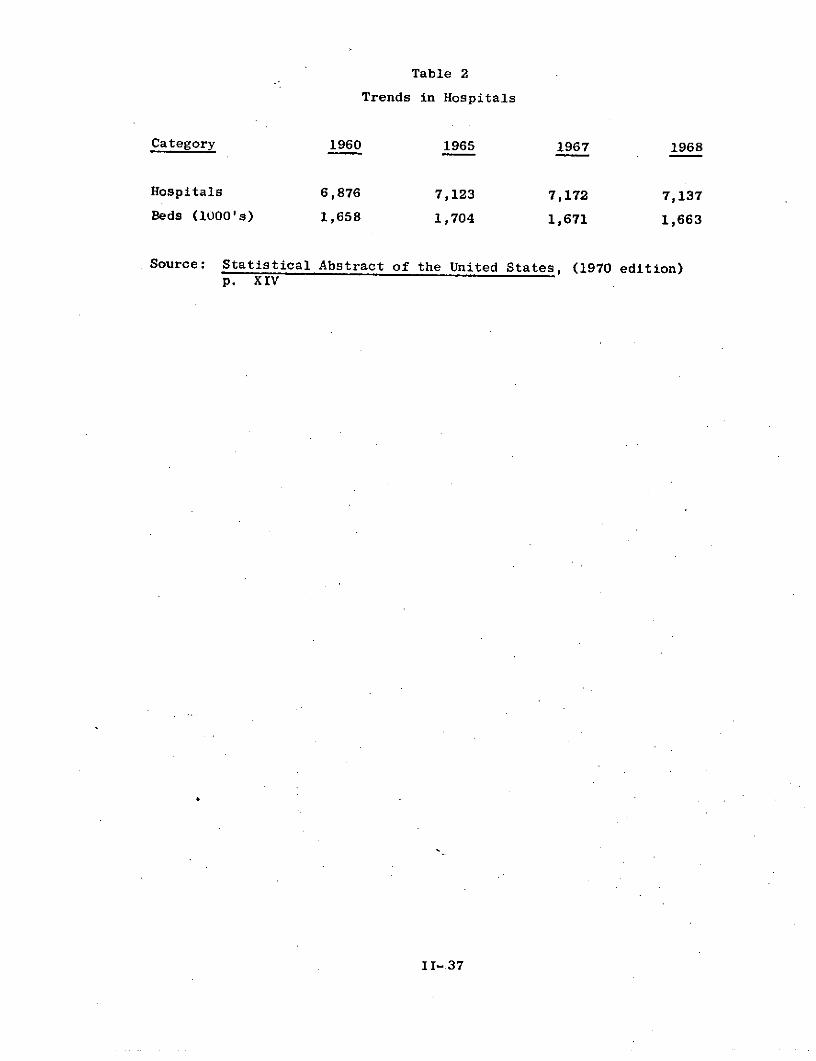
Table 2

Trends in Hospitals

Category 1960 1965 1967 1968

Hospitals 6,876 7,123 7,172 7,137

Beds (1000's) 1,658 1,704 1,671 1,663

Source: Statistical Abstract of the United States, (1970 edition)p. XIV

I-37

Table 3

Inpatient Health Facilities

Facility 1967 1968

Total Facilities 30,586 30,911

Hospitals 8,147 7,991

General Medical & Surgical 6,685 6,539

Specialty 1,462 1,452

Psychiatric 573 494Geriatric 333 291Tuberculosis 169 129Other 387 538

Nursing Care & Related Homes 19,141 19,500 est.

Nursing Care 10,636 (NA)

Personal Care, With NursingCare 3,853 (NA)

Personal Care, WithoutNursing Care 4,396 (NA)

Domiciliary Care 256 (NA)

Other 3,298 3,500

Source: Health Manpower and Health Facilities, 1969, p. 242, Table 169

II-38

section, the distribution of hospitals by bed size will be discussed.

Turning to the rural case, the number of remote villages in Alaska

has been estimated at 360 (Reference 9). Thus, Alaska

will need a substantial communication system if teleconferenced

medical care is to be provided for these villages. As will be discussed

in the case studies, about 75% of places under 2,500 in population, in

Colorado, do not have a single doctor. Although this study has only

been able to scratch the surface of the need for remote medical

services, such figures indicate that a substantial effort in this

direction is warranted.

There are about 300,000 doctors in America. If the results of the

San Jose, Denver and Salt Lake City case studies are indicative of a

general trend, then most doctors are located in metropolital areas,

although the bulk of them practice alone and a substantial number

are located relatively far from main clusters.

II-39

b. Continuing Professional Education

As shown previously in Table 1, there are between fifteen and twenty

five million "professional" workers in the United States. It is difficult

to provide a more exact figure, because the definition of "professional"

is somewhat ambigious. For example, 8 million workers are listed as

managers, proprietors and other officials," but how many of these workers

are truly professional can only be conjectured. From Table 4, the fact

that only 22% of these managers have completed 4 or more years of college

indicates that most of these managers are only semiprofessional--at least

in the sense that they would probably not be interested in obtaining

advanced intensive training (such as an M.B.A.). On the other hand,

Table 4 illustrates that other labor categories are fairly large. In

such categories as "craftsmen," a substantial number of workers might be

included who could benefit from vocational training that could best be

categorized as "professional."

In addition to the absolute number of professionals in each category

listed in Table 1, it is also necessary to determine how fast employment

in these fields is growing. A high growth rate indicates a dynamic

field and a younger population of workers. In Table 5, projected growth

rates are given for elementary and secondary school teachers. In Table 6

this information is given for teachers in higher education. Growth rates

for other selected fields are given in Table 7. Note especially the large

growth rates in nursing and teaching which are two of the largest pro-

fessional fields.

II-40

Table 4

Occupations of Employed Persons18 Years Old and Older (May 1969)

Average* 4 or More*Years of Some* Years ofCategory Number Schooling College College

Professional, Technical & Kindred 10,700,000 16.5 78% 60%Managers, Officials & Proprietors,

Except Farm 8,000,000 12.8 41% 22%Clerical & Kindred 12,400,000 12.6 30% 8%Salesworkers 4,800,000 12.8 42% 17%Craftsmen, Foremen & Kindred 11,100,000 12.1 11% 2%Operatives & Kindred 11,200,000 11.4 7% 1%Service Workers, Including Private

Households 8,900,000 12.1 15% 2%Farmers, Farm Managers, Laborers

& Foremen 2,900,000 9.4 9% 3%Laborers, Except Farm & Mine 4,400,000 10.5 8% 1%

*Figures for White Males Only

Source: Digest of Educational Statistics, 1970, p. 14, Table 17

II-41

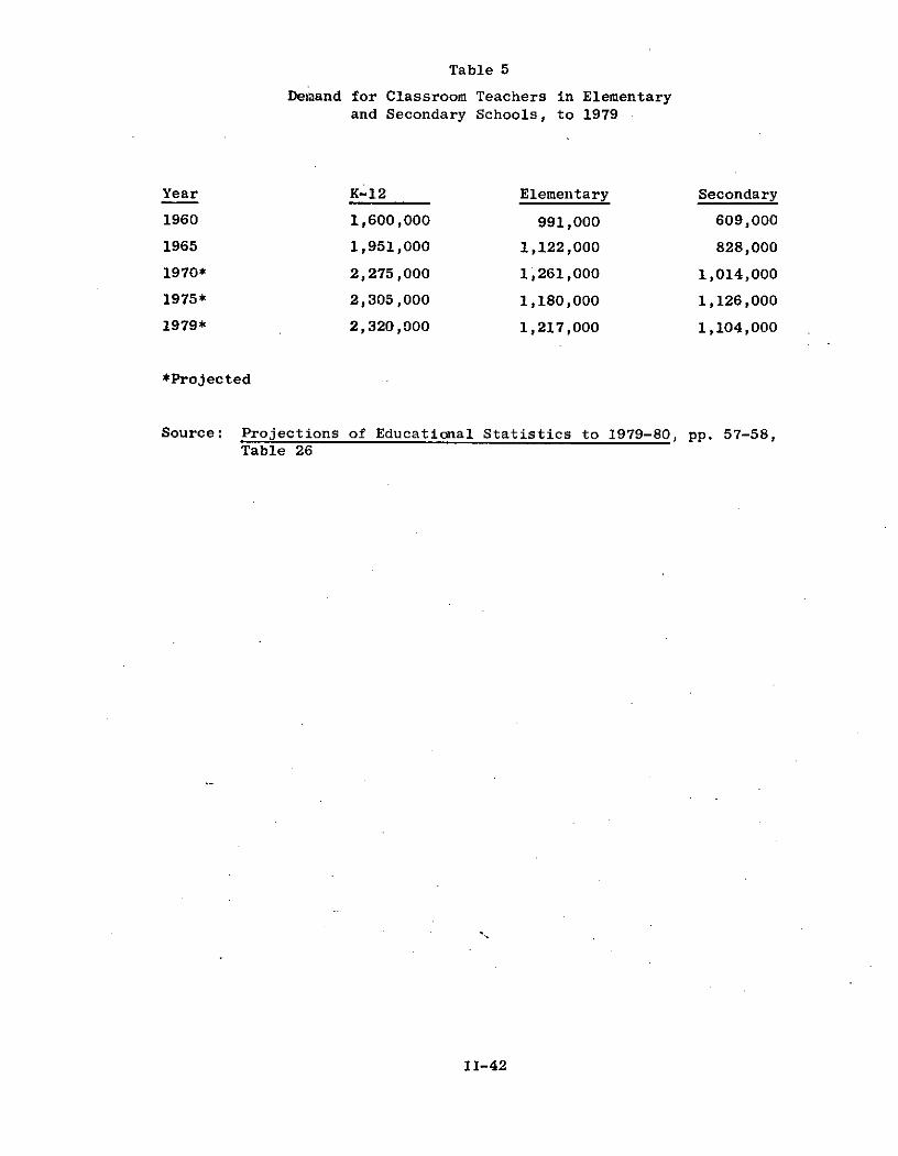
Table 5

Demand for Classroom Teachers in Elementaryand Secondary Schools, to 1979

Year K-12 Elementary Secondary

1960 1,600,000 991,000 609,000

1965 1,951,000 1,122,000 828,000

1970* 2,275,000 1,261,000 1,014,000

1975* 2,305,000 1,180,000 1,126,000

1979* 2,320,000 1,217,000 1,104,000

*Projected

Source: Projections of Educational Statistics to 1979-80, pp. 57-58,Table 26

II11-42

Table 6

Demand For Instructional StaffIn Higher Education

Instructor or Above

Jr.Year Total Total Full-Time Part-Time Instr.

1964-65 391,000 332,000 222,000 110,000 59,0001969-70 578,000 491,000 328,000 163,000 87,0001971-72* 592,000 603, 000 336, 000 167, 000 89, 0001979-80"* 801,000 681,000 455,000 226,000 120,000

*estimated

Source: Projections of Educational Statistics to 1979-80,. bb.-4

II-43

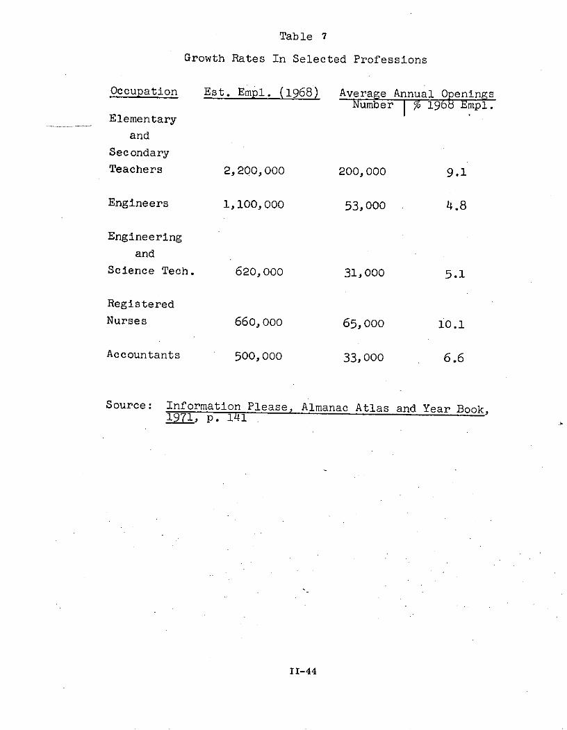
Table 7

Growth Rates In Selected Professions

Occupation Est. Empl. (1968) Average Annual OpeningsNumber I 1968 Empl.

Elementary

and

Secondary

Teachers 2,200,000 200,000 9.1

Engineers 1,100,000 53,000 4.8

Engineering

and

Science Tech. 620,000 31,000 5.1

Registered

Nurses 660,000 65,000 10.1

Accountants 500,000 33,000 6.6

Source: Information Please, Almanac Atlas and Year Book,1971, p. 141

II-44

There are two types of continuing professional education, namely

degree-oriented and general. All professionals need general education,

which allows them to keep abreast of current developments, review past

learning, and pick up new competences. Degree-oriented education is a

more restricted market. For example, doctors, lawyers and other profes-

sionals who have reached terminal degrees (such as M.D., L.L.B., M.B.A.)

have no need for degree-oriented education, unless they are changing

fields or are planning to go into specialized work, such as research or

teaching. For other groups, it is desirable to know the percentage of

workers having non-terminal bachelors or masters degree. In Table 8,

such information is presented for scientists in general. Note that

30% have only a bachelor's degree, and about an equal number have a

masters's. Information on the number of employed persons who could

benefit from degree education is difficult to estimate. The managerial

category, for example, has need for M.B.A.'s bachelor's degrees and special

certificate programs.

In the following sections on the use of demography for demand

assessment, no attempt was made to develop complete profiles of the

various categories. Time did not allow all of this information to be

gathered, and much of it does not exist in convenient form. Rather the

emphasis was upon presenting the important demographic variables which

must be considered by system designers.

II-45

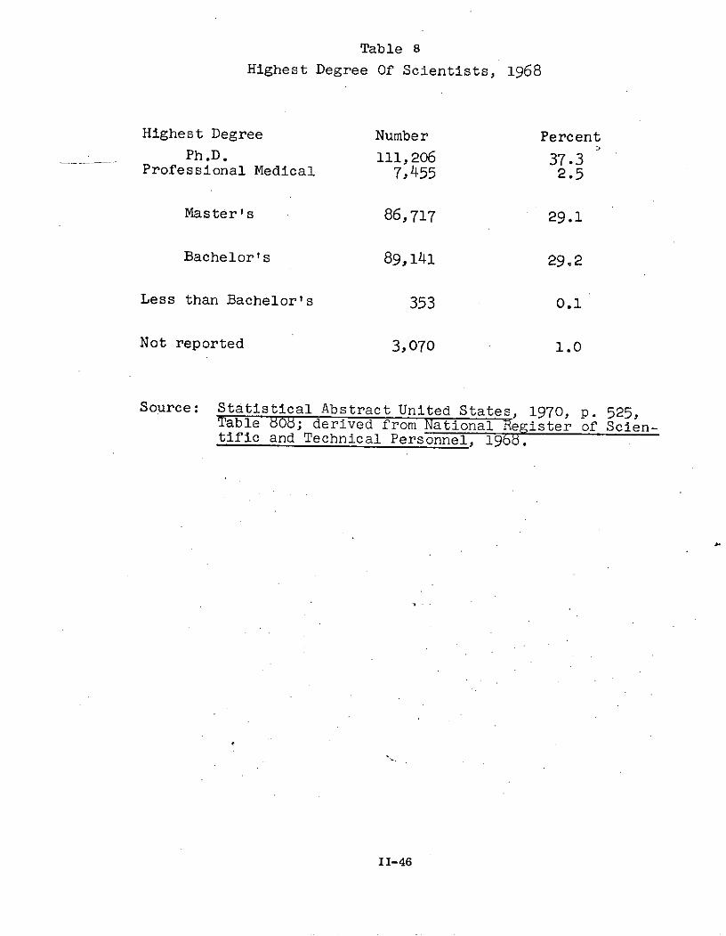
Table 8

Highest Degree Of Scientists, 1968

Highest Degree Number Percent

Ph.D. 111,206 37.3Professional Medical 7,455 2.5

Master's 86,717 29.1

Bachelor's 89,141 29.2

Less than Bachelor's 353 0.1

Not reported 3,070 1.0

Source: Statistical Abstract United States, 1970, p. 525,Table 80b; derived from National Register of Scien-tific and Technical Personnel, 1968.

II-46

2. System Design

Demography helps system designers determine such things as the

number of channels they will need for a given application. System designis largely dependent upon the clustering of users. If users are located

in the same building, for example, a single receiver could be used forsatellite reception, and its cost spread over the number of people served.Or, if user population in the area is generally high, cables become moreattractive relative to ITFS, than if user density is low.

The demographics of health services are relatively straightforward.

The number of hospitals must be known, as must the number and location ofphysicians, the remote villages to be served, and the desired number ofghetto clinics. Adequate listings of doctors and hospitals are available,as is other information (although sometimes difficult to locate).

The demographics of continuing professional education are less well-defined. To start with, the designer must decide whether the system willserve individuals at their place of work, or whether it will serve all ofthe professionals who work in a given plant. The former might be calleda people orientation and the latter an industry orientation. Ultimately,as the professional group vs. industry matrix becomes disaggregated, thisdistribution will become meaningless. In the near future, however, systemsare likely to be established by professional societies or industries, andthe distinction will be an important one. In addition to this difficulty,demographers will find that few professions are adequately described instandard data sources. Engineers, for example, are spread across manufac-turing, civic services, government, and a host of other jobs. Designinga people-based system for engineers (as was essentially done with theStanford ITFS system) might be attractive from the standpoint of an aca-demic department of a university, but demographic information for such asystem is virtually nonexistent.

II-47

a. People-Based Systems

Groups such as professional societies would probably seek de very

systems which serve specific work groups, for example engineers. In

order to design systems like this, it is essential to know the

geographical distribution of the target population. At the first

level, it would be desirable to know distributions by state. Table 9,

taken from the Statistical Abstract of the United States (1970 Edition),

illustrates some of the pitfalls of loose reasoning on geographical

distributions. In the original table, the number of professional

scientists in a large number of categories was given, by state. In

Table 9, only physicists, chemists and atmospheric and earth scientists

are listed. Suppose a system designer had only figures for physicists,

and tried to extrapolate this information to other fields. Then his

estimates of the number of chemists in New Jersey, for example, would

be off by a factor of three. And the estimated number of atmospheric

and earth scientists would be off by a factor of almost six.

Just as professionals cluster by state, they also cluster by regions

within a state. In our first demographic case study, electronic manufac-

turers in the San Francisco Bay Area were located on a map. Because ITFS

delivery was contemplated, only employers with 20 or more engineers were

plotted. Note in this figure the heavy concentration around Palo Alto

(where Stanford is located), and the lack of plants in large areas like

San Francisco and Oakland. Such clustering makes systems like cable or

ITFS relatively attractive, while dividing the number of engineers in

II-48

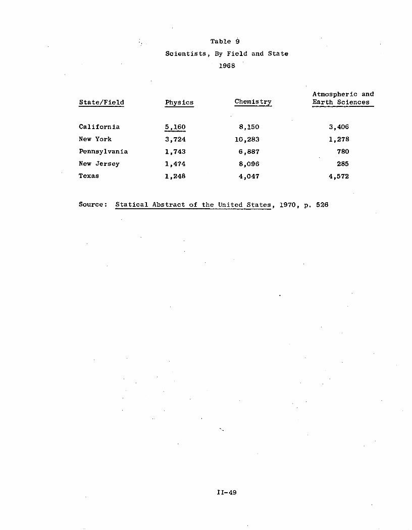
Table 9

Scientists, By Field and State

1968

Atmospheric and

State/Field Physics Chemistry Earth Sciences

California 5,160 8,150 3,406

New York 3,724 10,283 1,278

Pennsylvania 1,743 6,887 780

New Jersey 1,474 8,096 285

Texas 1,248 4,047 4,572

Source: Statical Abstract of the United States, 1970, p. 526

II-49

the state by the total area in the state would make direct satellite

reception appear to be necessary.

On an even smaller scale, professionals have varying tendencies to

cluster in sections of metropolitan areas. In the Denver and Salt Lake

City cases, doctors and lawyers were found to cluster in the central

cities, with suburban areas being poorly served. The Denver case,

however, illustrates the danger of extrapolation between professions.

While doctors and lawyers were found to cluster in central cities to

a greater extent than general population, teachers seemed to be more

evenly distributed (although the quality of the data was poor on this

point). Thus, different professional groups tend to cluster differently

relative to population, within a region.

Within a central city, one would expect to find further clustering

of professionals. The San Jose case demonstrated that doctors tend to

be clustered primarily in downtown areas and near hospitals. Lawyers

were also concentrated downtown. Other pockets of both professional

groups were also found (the pockets did not coincide), the causes of

which could not be determined from the analysis. In the San Jose case,

a cable run of approximately 55 miles would serve about 95% of the doctors,

while 85 miles of cable would have been necessary to serve all. The

figures on lawyers were similar. Concentration, then, is a two-edged sword.

It makes systems like cable relatively attractive, buy the marginal

cost of adding outlying professionals to such systems is inordinately high.

II-50

The last level of clustering is concentration within a building.

Because teachers work within schools, a single terminal system can

normally serve 5 to 150 teachers. This allows the cost of the receiver

and other interface devices to be spread over many users. Similar

economies of concentration would exist for engineers in a research

organization. For doctors and lawyers, the amount of clustering is not

a priori apparent. Both groups tend to work in professional buildings,

which are shared by other professional groups. A preliminary indication

on the clustering of doctors was found in the San Jose case study. The

data were not accurate enough to determine concentration by building,

they yielded the result that if there was any doctor on a block, the

average number of doctors on that block was 3.3. This is a fair degree

of clustering, but its significance should not be overestimated. Large

clusters (on the order of 50 doctors) in major clinics tend to suppress

the number of doctors in solo practice in the concentration statistic.

The fact that some doctors work in group practive or near other doctors

while others work alone poses questions for the pricing of services. If

receivers are sold, then doctors in solo practive will probably not be

able to afford them. A more desirable policy might be to base charges

on the number of hours of system use.

For professions in which people are normally employed by organizations,

it is necessary to know what portion of the professionals are employed

in each type of industry. Tables 10,11, and 12 present such information

II-51

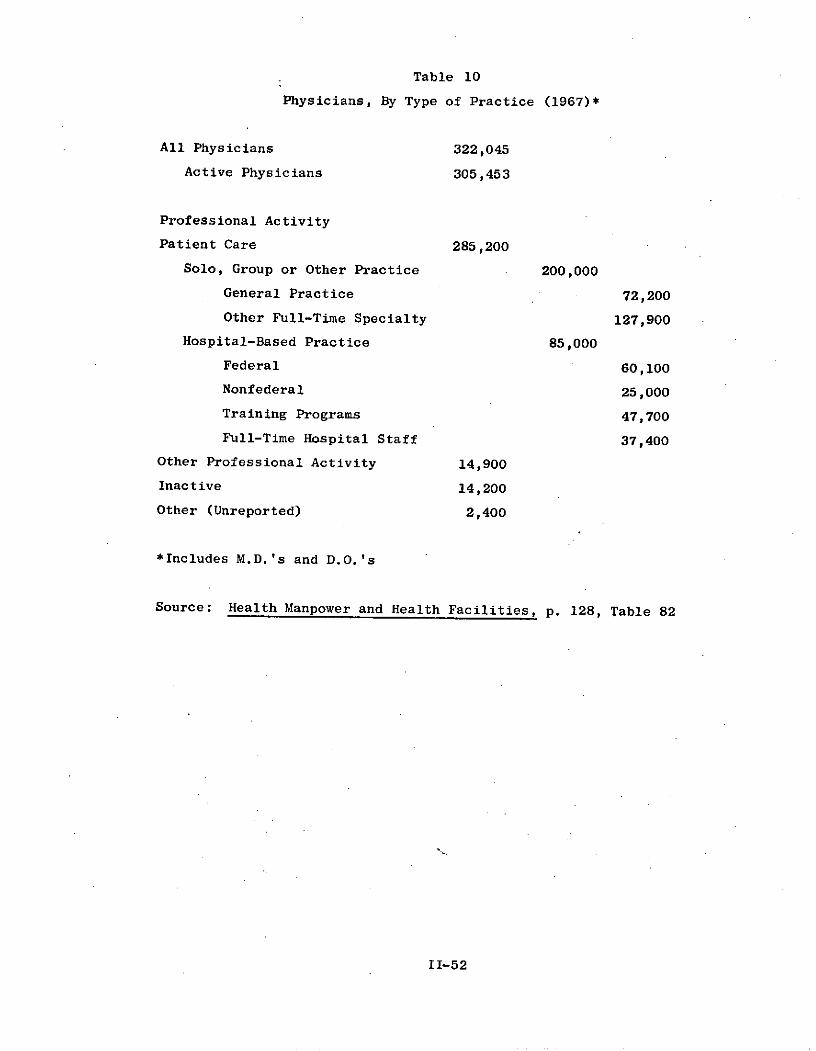
Table 10

Physicians, By Type of Practice (1967)*

All Physicians 322,045

Active Physicians 305,453

Professional Activity

Patient Care 285,200

Solo, Group or Other Practice 200,000

General Practice 72,200

Other Full-Time Specialty 127,900

Hospital-Based Practice 85,000

Federal 60,100

Nonfederal 25,000

Training Programs 47,700

Full-Time Hospital Staff 37,400

Other Professional Activity 14,900

Inactive 14,200

Other (Unreported) 2,400

*Includes M.D.'s and D.O.'s

Source: Health Manpower and Health Facilities, p. 128, Table 82

II-52

Table 11

Fields of Employment of Registered Nurses (1967)

Field of Employment No. Nurses % of Total

Total 659,000 100.0%

Hospitals, Nursing Homes andRelated Functions 452,500 68.7

Hospitals 361,100* 55%

Nursing Homes, etc. 91,500' 14%

Public Health & Schools 47,100 7.1

Occupational Health 19,600 4.2

Private Duty, Office & Other Fields 112,200 17.0

*1966 Data (HM&HF, 1969, p. 22)

'By Calculation (452,500 - 361,100)

Source: Health Manpower & Health Facilities (1969) p. 146, Table 93

11-53

Table 12

Scientists In Private Industry By Industry, 1967

Industry Total Engineers Mathematicians Chemists Physicists Life Scientists. Technicians

All 1,747,800 824,000 31,300 85,200 16,200 22,400 737#700

Chemicals & AlliedProducts 140,200 42,500 1,400 40,500 2,100 11,200 40,800

Petroleum Refining 20,000 10,700 200 3,300 100 less than 50 6,200

Primary & Fabrica-

ted Metal Products 105,000 50,600 1,000 3,200 400 100 44,000

Machinery 166,400 81,500 3,200 1,800 600 200 77,800

Communications &

Equipment 115,600 68,100 1,900 600 1,300 100 42,900

Aircraft & Parts 131,600 84,500 3,600 2,100 1,400 200 38,200

Motor Vehicles &

Equipment 50,300 29,300 500 800 200 less than 50 18,800

Instruments & Rela-ted Products 60,600 32,400 500 3,500 1,000 200 22,500

Other Manufacturing 115,600 52,200 1,300 13,400 500 3,900 42,300

Trans., Public Utili-

ties, Other Manufact. 206,080 82,500 7,500 4,800 300 3,200 107,600

Services 298,500 103,500 4,400 6,800 4,000 2,800 173,200

Source: Statisoal Abstract of the United States, 1970, p. 523

II-54

for doctors, nurses, and scientists. For these fields, data is available.

For other fields, information is seldom in manageable form. For

example, accountants are spread through corporations in functional roles.

Even in the case of scientists and engineers (Table 12), available

information is relatively coarse grained and of limited utility to system

designers.

II-55

b. Industry-Based Systems

Three types of information is necessary in the design of industry-

based systems. First, the number of people and work locations in.the

industry should be known. Second, it is necessary to know what types

of professionals work in the industry. Finally, it is necessary to know

the distribution of sizes of the working locations, at which professionals

will receive services.

There is a great deal of scattered information on the first topic.

For example, if the military were selected, about 3.5 million people

would be in the total population. Table 13 lists the number of people

employed in Federal, state and local jobs. Table 14 lists the number of

banking and other financial units in the United States. Tables 15 and 16

provide the number of school systems and institutions of higher education,

respectively. The next matter is determining what professional groups

work in a given industry. Table 17 presents the breakdown of professionals

and other classes in hospitals. Table 18 presents similar information

concerning nursing homes. For other industries, information is usually

more difficult to obtain, because classifications vary from organization

to organization. The data from which Table 12 (scientists, by profession

and industry) provides somewhat crude information for scientists and

engineers.

The last problem is to determine the distribution of sizes of basic

working units. In Table 15, the size distribution of school systems is

II-56

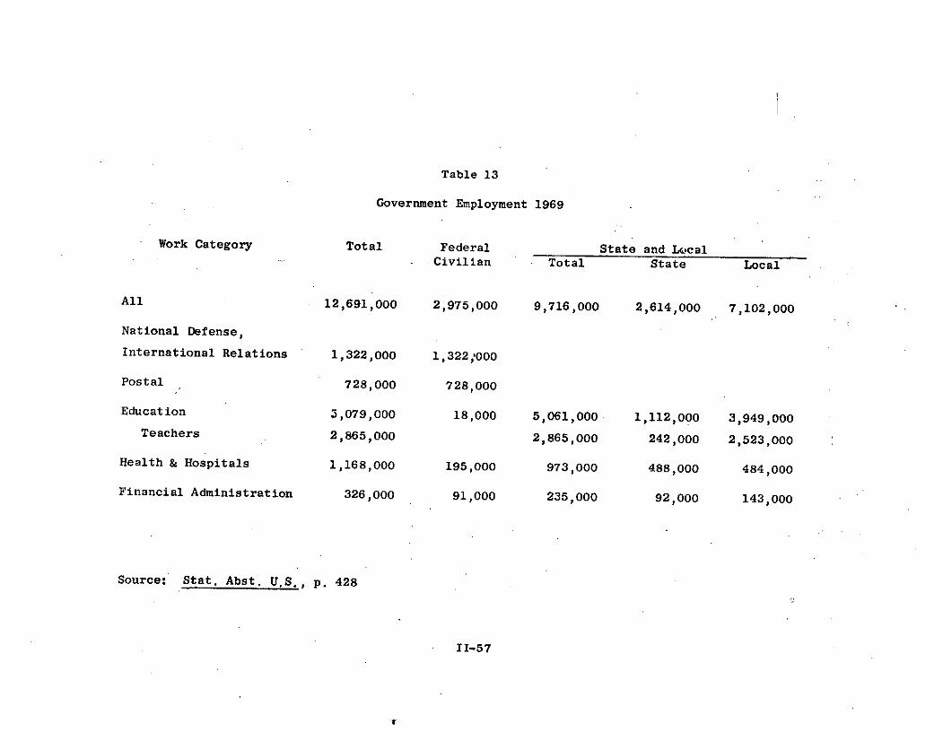
Table 13

Government Employment 1969

Work Category Total Federal State and LecalCivilian Total State Local

All 12,691,000 2,975,000 9,716,000 2,614,000 7,102,000

National Defense,

International Relations 1,322,000 1,322;000

Postal 728,000 728,000

Education 3,079,000 18,000 5,061,000 1,112,000 3,949,000Teachers 2,865,000 2,865,000 242,000 2,523,000

Health & Hospitals 1,168,000 195,000 973,000 488,000 484,000

Financial Administration 326,000 91,000 235,000 92,000 143,000

Source: Stat. Abst. U.S., p. 428

II-57

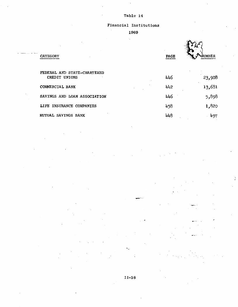
Table- 14

Financial Institutions

1969

CATEGORY PAGE ' ER

FEDERAL AND STATE-CHARTEREDCREDIT UNIONS 446 23,908

COMMERCIAL BANK 442 13,681

SAVINGS AND LOAN ASSOCIATION 446 5,898

LIFE INSURANCE COMPANIES 458 1,820

MUTUAL SAVINGS BANK 448 497

II-58

Table 15

Number of Public School Systems

by Size of System: 1966-67

ENROLLMENT SIZE SCHOOL SYSTEMS PUPILS ENROLLEDNUMBER PERCENT NUMBER (X 1000) PERCENT

TOTAL 23, 390 100.0 43,842 100.025,000 or MORE 170 .7 12,590 28.712,000 to 23,999 350 1.5 5,730 13.16,000 to 11,999 880 3.8 7,293 16.6

3,000 to 5,999 1,726 7.4 7,178 16.41,800 to 2,999 1,819 7.8 4,251 9.71,200 to 1,799 1,636 7.0 2,416 5.5600 to 1,199 2,838 12.1 2,437 5.6

300 to 599 2,723 11.6 1,185 2.7150 to 299 2,091 8.9 459 1.0

50 to 149 2,230 9.5 209 0.5

15 to 49 2,673 11.4 71 .2

1 to 14 2,386 10.2 22 .1

NONE(NOT OPERATING) 1,868 8.0

SOURCE: Description of Educational Statistics, 1970, p. 44

II-59

Table 16

Number of Institutions of Higher Education.Fall 1969

Size of Enrollment All Institutions Universities All Other 4-Year 2-Year

Institutions Institutions

Number Enrollment No. E. No. E. No. E.

All 2,525 7,916,991 159 2,879,847 1480 3,094,819 886 -1,942,325

Under 200 273 29,693 183 20,055 90 9,638

200 - 499 369 128,346 204 71,138 165 57,208

500 - 999 570 421,139 379 280,243 191 140,896

1,000 - 2,499 618 966,425 2 4,075 392 611,588 224 350,762

2,500 - 4,999 287 1,019,495 10 42,138 163. 575,446 114 401,911

5,000 - 9,999 229 1,656,757 50 387,051 112 808,447 67 461,257

10,000 - 19,999 114 1,589,323 47 710,038 36 461,243 31 418,042

20,000 - 29,999 39 924,830 25 587.,913 10 234,308 4 102,609

30,000 or more 26 1,180,983 25 1,148,632 1 32,351

Source: Digest of Educational Statistics, 1970, p. 85

II-60

Table 17

Employment in Hospitals} 1966

Occupation Medical Total Hospitals

All 3,672,000 2,363,000

Profl. & Tchnl. 1,487,100 860,000

Engr. & Nat. Sci. 23,200 11,300

Dentists 94,900 900

Dietitians & Nutritionists 18,200 13,200

Reg. Nurses 584,100 395,900

Optometrists 13,900 500

Pharmacists 10,600 9,200

Physicians (MD's &DO's) 254,500 59,100

Chiropractors & Therapists 54,900 18,900

Med & Dent Technicians 203,600 140,100

Socl. & Welfare Wkers 15,800 10,600

Other 213,400 200,400

Mgrs., Offcls., & Proprietors 94,400

Clerical 596,700 280,300

Service 1,310,200 1,022,000

Aides, Orderlies, Attendants 637,900 516,500

Cooks 50,700 37,100

Prac. Nurses 254,800 150,100

Janitors & Cleaners 79,400 49,900

Other. 287,400 268,400

Other 183,600 148,100

Source: Stat. Abst. U. S., p. 64, -1970

II-61

Table 18

Full-Time Personnel in Nursing and Personal Care Facilities: April-July 1968

Nursing PersonalCategory of Personnel Total Nuare Care

Total Professional and Technical 279,288 229,937 49,351

Nursing Services:

Nurse - R.N. 25,139 21,263 3,876Licensed practical nurse or vocational nurse 35,725 29,561 6,164Aide, Orderly, Attendant 186,411 155,315 31,096

Therapeutic Services

Physical Therapist 944 846 98Physical Therapy Assistant 1,411 1,238 173Recreational Therapist 1,743 1,385 358Registered Occupational Therapist 450 373 77Other occupational therapists and assistants 1,269 1,058 211Social Worker

722 571 151Speech Therapist 86 77 9

Medical Records

Registered medical record librarian 192 158 34Other medical records librarians & technicians 948 818 130

Dietary:

Dietitian 3.082 2,087 995

All other professional and technical 21,166 15,187 1,633

Source: Health Manpower and Health Facilities, 1969, p. 23, Table 12

II-62

given. This is important for administrative purposes, but a better

statistic would be the number of teachers in each school. Such ijfformation

is seldom available in closed form. The Denver case study presents such

information for teachers, although the base data was not ideal. Table 19

lists the distribution of units under social security. For larger

units, this data is insufficient, because it is necessary to know how

many buildings the workers are staffed in, in order to determine the

number of receivers necessary. Table 20 lists hospitals, by bed size.

II-63

Table 19

Reporting Units Under Social Security (1968)

Industry1-3 4-7 8-17 20-49 50-99 100-249 250-499 500 or more

Reporting Units 1,815,244 708,594 568,762 252,021 84,443 48,104 15,343 10,942% of Total 51.8 20.2 16.2 7.2 2.4 1.4 0.4 0.3Employees (xlO00) 3,142 3,671 6,779 7.572 5,793 7,297 5,281 14,911% of Total 5.8 6.7 12.5 13.9 10.6 13.4 9.7 27.4

Agriculture,Forestry &Fisheries 19,230 6,719 4,099 1,323 294 93 16 1Mining 9,689 4,591 5,652 3,480 1,150 645 223 130Contract Const. 160,065 66,107 51,344 21,562 6,735 2,970 562 195Manufacturing 71,608 48,183 66,051 51,094 29,351 20,855 8,129 6,189Trahsportation &*Other Public Util-ities 53,830 23,878 25,323 13,827 5,400 3,222 982 803

Wholesale Trade 115,582 68,283 71,246 32,637 8,409 3,147 552 221Retail Trade 523,408 247,846 183,553 64,536 16,098 6,376 1,683 11,131Finance, Insur-ance and RealEstate 213,156 53,102 37,192 16,335 5,146 2,864 814 557Services 598,220 176,888 116,344 45,148 14,838 7,932 2,382 1,733Unclassified 50,456 12,997 7,958 2,079 22 - - -

8ourcel Statistical Abstract of the United States, 1970, p. 472

11-64

Table 20

Bed Size of Hospitals, 1968

General Med.Bed Size Total Hospitals And Surgical Specialty

All 7,991 6,539 1,452

Under 25 803 633 17025-49 1,826 1,597 229

50-74 1,085 908 17775-99 801 652 149

100-199 1,546 1,282 264200-299 704 6o8 96

300-499 653 571 82500-999 318 236 82

Over 1000 255 52 203*

*188 are psychiatric hospitals

Source: Health Manpower and Health Facilities, 1969, p. 247, Table 171

II-65

c. Summary

The purposes of the preceeding sections have been to give the'

reader an understanding of what types of demographic data are desirable,

a flavor of what information is available, and a feeling for the general

paucity of information in a form useful for system designers.

II-66

3. Case Studies in Demography

To illustrate the principles described above, and to provide

approximate population characteristics for the technological case studies,

six minor studies were conducted. They will be presented in the

remainder of this section, generally in order of increasing geographical

area (and correspondingly decreasing resolution). The exception to

this trend will be the first case, which explores the demographics of

a people-based delivery system.

Demographic information, even when available, is expensive to

process and normally contains little of theoretical interest. Because

the resources allocated to this study were limited, attempts were made

to focus on population groups for which information is readily available,

and to provide rough cuts at actual numbers. Although subject to

errors of fifteen to twenty five percent, the numbers would prove

sufficient accuracy for the technical case studies and also provide a

general picture of demographic trends.

II-67

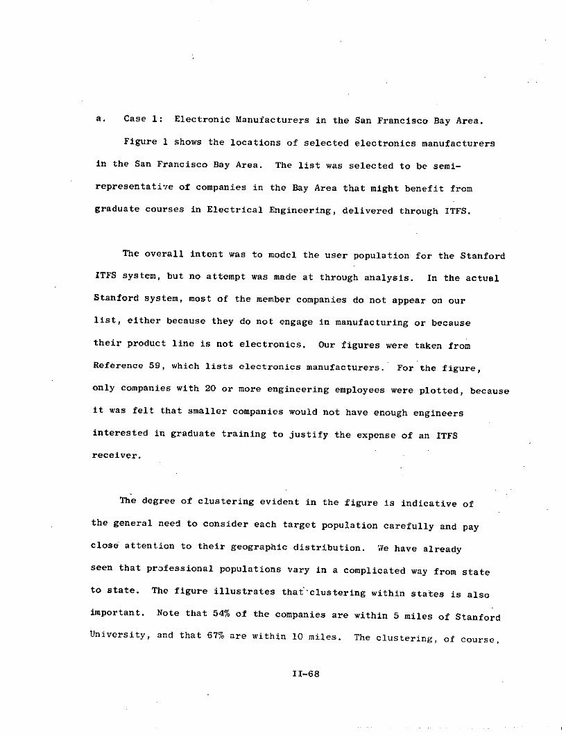
a. Case 1: Electronic Manufacturers in the San Francisco Bay Area.

Figure 1 shows the locations of selected electronics manufacturers

in the San Francisco Bay Area. The list was selected to be semi-

representative of companies in the Bay Area that might benefit from

graduate courses in Electrical Engineering, delivered through ITFS.

The overall intent was to model the user population for the Stanford

ITFS system, but no attempt was made at through analysis. In the actual

Stanford system, most of the member companies do not appear on our

list, either because they do not engage in manufacturing or because

their product line is not electronics. Our figures were taken from

Reference 59, which lists electronics manufacturers. For the figure,

only companies with 20 or more engineering employees were plotted, because

it was felt that smaller companies would not have enough engineers

interested in graduate training to justify the expense of an ITFS

receiver.

The degree of clustering evident in the figure is indicative of

the general need to consider each target population carefully and pay

close attention to their geographic distribution. We have already

seen that professional populations vary in a complicated way from state

to state. The figure illustrates thaftclustering within states is also

important. Note that 54% of the companies are within 5 miles of Stanford

University, and that 67% are within 10 miles. The clustering, of course,

II-68

RICHMONDI CONCORD

WALNUTBERKELEY CREEK

SANFRANCISCO OAKLAND

3

SANLEANDRO SAN

I RAMON

BELMONT

SANCARLOS

5MENLOPARK

PALOALTO

15MOUNTAIN

VIEWI10

SUNNYVALE5 SANTA

CLARA

CUPERTINO

SAN JOSE2

Figure 1: Electronics Manufacturing Companies Having 20 or More

Engineering Employees

II-69

is mainly caused by the presence of Stanford Engineering "communities"

also exist in other regions. In Santa Barbara, California, for instance,

there is a very large research and development concentration.

In Figure 2, the distribution of engineering employees by size of

firm is shown for electronics manufactureres in the Bay Area. It is

interesting to note that 35% of the engineers work in companies with

between 1000 and 2000 engineering employees, while 15% are employed by

companies having fewer than 100 engineers. About half of the engineers

are employed in companies with fewer than 400 engineers.

II-70

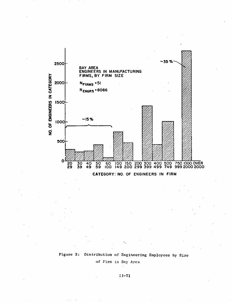
2500-35BAY AREAENGINEERS IN MANUFACTURING

>- FIRMS, BY FIRM SIZE00 2000- NFIRMS '51

I-5

NENGRS = 808 6

1500'-

1000- 15%

500 -

20 30 40 50 60 100 150 200 300 400 500 750 1000 OVER29 39 49 59 100 149 200 299 399 499 749 999 2000 2000

CATEGORY: NO. OF ENGINEERS IN FIRM

Figure 2: Distribution of Engineering Employees by Size

of Firm in Bay Area

II-71

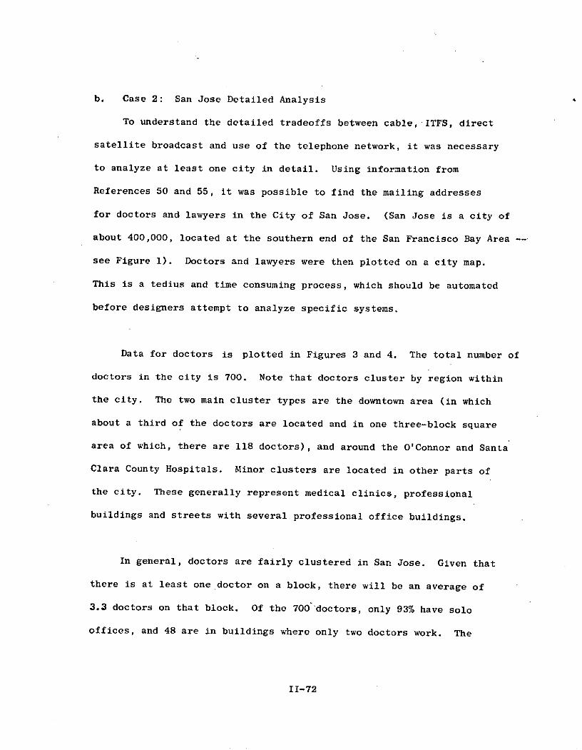
b. Case 2: San Jose Detailed Analysis

To understand the detailed tradeoffs between cable, ITFS, direct

satellite broadcast and use of the telephone network, it was necessary

to analyze at least one city in detail. Using information from

References 50 and 55, it was possible to find the mailing addresses

for doctors and lawyers in the City of San Jose. (San Jose is a city of

about 400,000, located at the southern end of the San Francisco Bay Area -

see Figure 1). Doctors and lawyers were then plotted on a city map.

This is a tedius and time consuming process, which should be automated

before designers attempt to analyze specific systems.

Data for doctors is plotted in Figures 3 and 4. The total number of

doctors in the city is 700. Note that doctors cluster by region within

the city. The two main cluster types are the downtown area (in which

about a third of the doctors are located and in one three-block square

area of which, there are 118 doctors), and around the O'Connor and Santa

Clara County Hospitals. Minor clusters are located in other parts of

the city. These generally represent medical clinics, professional

buildings and streets with several professional office buildings.

In general, doctors are fairly clustered in San Jose. Given that

there is at least one doctor on a block, there will be an average of

3.3 doctors on that block. Of the 700 doctors, only 93% have solo

offices, and 48 are in buildings where only two doctors work. The

II-72

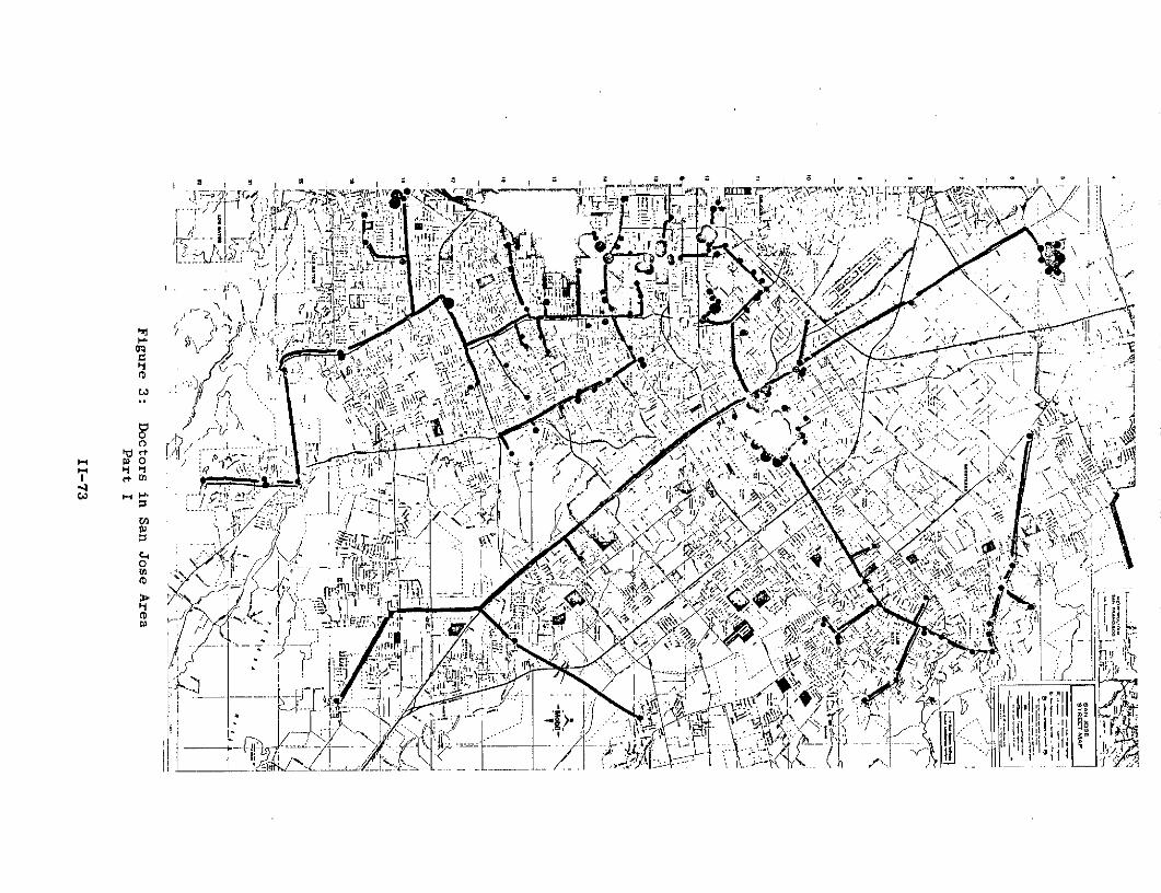
A " ' , -- I q -/ - '

-- 1-.1 - ' III; r~

P 3A

-J

o.- I I I ~is;IW1 .'. Y IJ ' ;1' r

(D ~ '

0 ...... i :I -F

P1i

ELI\

fi ~i ,,Aua - i tcl .. L .3 rko ,'ME

/71 :

6 :S M '

-b ~ q 1A4 L ~ EA

/A

4,, f ~} 31~j -I 1hl

aq30

C:

b110CD L

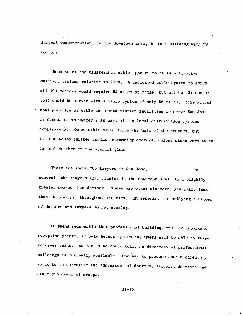
largest concentration, in the downtown area, is in a building with 59

doctors.

Because of the clustering, cable appears to be an attractive

delivery system, relative to ITFS. A dedicated cable system to serve

all 700 doctors would require 85 miles of cable, but all but 39 doctors

(6%) could be served with a cable system of only 55 miles. (The actual

configuration of cable and earth station facilities to serve San Jose

is discussed in Chaper 7 as part of the local distribution systems

comparison). Hence cable could serve the bulk of the doctors, but

its use would further isolate community doctors, unless steps were taken

to include them in the overall plan.

There are about 700 lawyers in San Jose. In

general, the lawyers also cluster in the downtown area, to a slightly

greater degree than doctors. There are other clusters, generally less

than 15 lawyers, throughout the city. In general, the outlying clusters

of doctors and lawyers do not overlap.

It seems reasonable that professional buildings will be important

reception points, if only because potential users will be able to share

receiver costs. As far as we could tell, no directory of professional

buildings is currently available. One way to produce such a directory

would be to correlate the addresses of doctors, lawyers, dentists and

other professional groups.

II-75

c. Case 3: Doctors in the Salt Lake City Metropolitan Area

San Jose might be termed a "central city," relative to other

communities near it. It seems plausible that such cities will have

different professional characteristics than surrounding urbanized areas

of the same size. To evaluate this conjecture, an analysis was made

of doctors in the area defined in the 1970 census as the Salt Lake City

Metropolitan Area. Unlike standard metropolitan statistical areas

(SMSA's), metropolitan areas are defined in terms of central cities,

plus surrounding densely settled areas. The Salt Lake City Metropolitan

Area (SLCMA) is shown in Figure 5.

Table 21 lists the populations of cities within the SLCMA, the

number of doctors in each, and the number of doctors per 1000 residents.

Again, business mailing addresses were used. The surprising result is

the high clustering of doctors in the central city. 93% of the doctors

are located in Salt Lake City, which contains less than half of the

population of the region. Note also that East Mill Creek, a city of

27,000 people, does not have a single doctor.

II-76

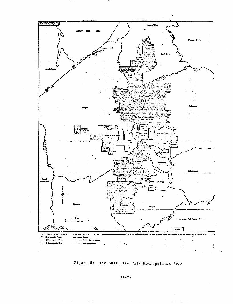
•s/ LO" .

OATALT LATE IATY'

....... ... .

, - -~..m e~ .....--- .~-m "

/ Oi.

. . . . ............... ...

/. .

- I ./r.,:' 0 "

b... ..... - . .

".-.4.. L ..

Figure 5: The Sal Lke City Metropoltan Area

SL CI-77IT

0. . N... I

.cc

DMt.

A U FcA rcwt G-0

i --- ~"'"'" "'--I"

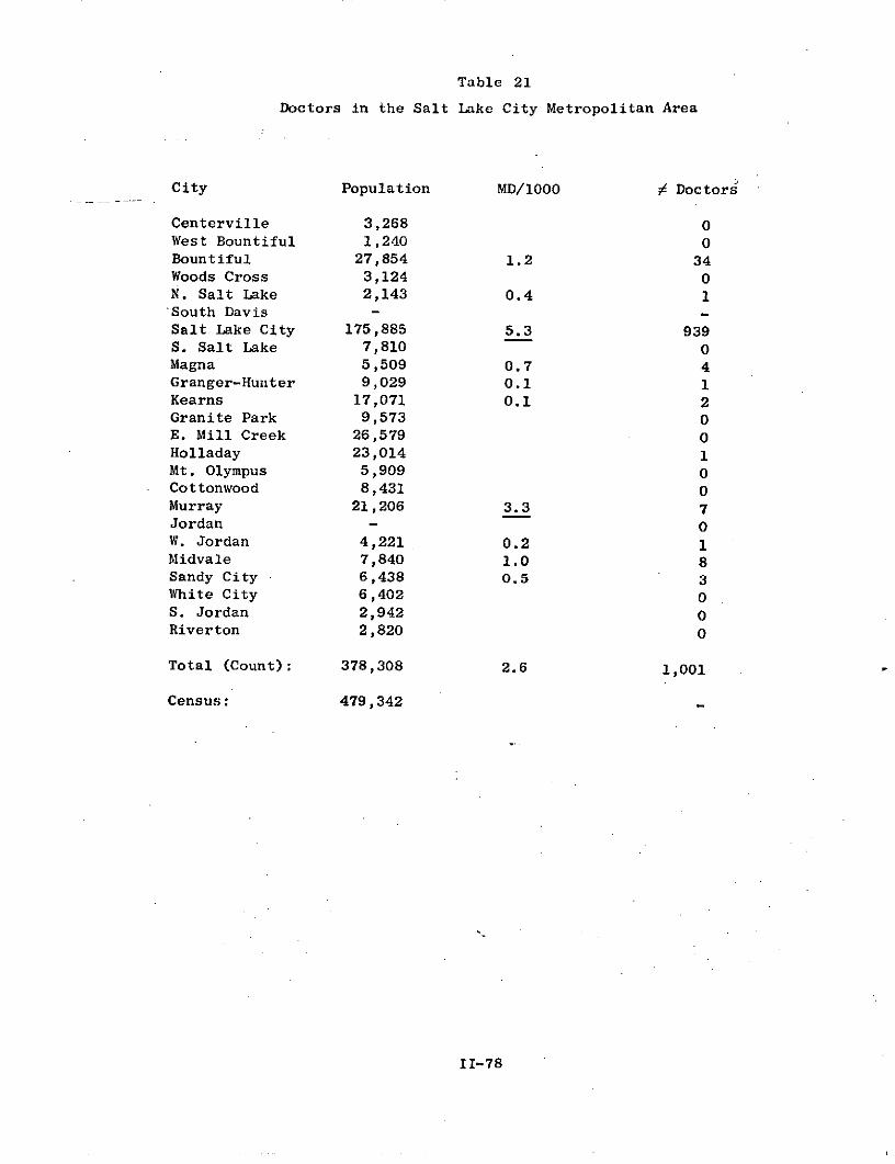
Table 21

Doctors in the Salt Lake City Metropolitan Area

City Population MD/1000 f Doctors

Centerville 3,268 0West Bountiful 1,240 0Bountiful 27,854 1.2 34Woods Cross 3,124 0N. Salt Lake 2,143 0.4 1South Davis -Salt Lake City 175,885 5.3 939S. Salt Lake 7,810 0Magna 5,509 0.7 4Granger-Hunter 9,029 0.1 1Kearns 17,071 0.1 2Granite Park 9,573 0E. Mill Creek 26,579 0Holladay 23,014 1Mt. Olympus 5,909 0Cottonwood 8,431 0Murray 21,206 3.3 7Jordan - 0W. Jordan 4,221 0.2 1Midvale 7,840 1.0 8Sandy City 6,438 0.5 3White City 6,402 0S. Jordan 2,942 0Riverton 2,820 0

Total (Count): 378,308 2.6 1,001

Census: 479,342

II-78

d. Case 4: Doctors, Lawyers and Teachers in the Denver Metropolitan Area

The Denver Metropolitan Area (DMA) is shown in Figure 6. The

populations of cities, number of doctors in each, and number of lawyers

in each are shown in Table 22. As in the case of the SLCMA, doctors

cluster in the central city of Denver. 86% of the doctors are in

Denver, which contains about half of the area's population. Also as in

the case of the SLCMA, there are several cities with populations over

10,000 which do not have any doctors. Medical populations in the suburbs,

however, are not uniform. North Glen (27,937), for example, has only

one doctor, while Littleton (26,466) has sixty.

Lawyers were also found to cluster in Denver (85%), and their

populations in other cities closely paralleled those of doctors (with

the exception of Golden, which has much legal activity).

Parallel data on schools could not be found, because school

districts did not follow city boundaries, and there was not enough

time to plot each school on maps. The Denver school district, however,

did cover only Denver, and the number of teachers there (4716) provide

some comparison to doctors (2251) and lawyers (2726). Nationally, there

are almost 10 times as many teachers as doctors or 2awyers, so these

figures indicate that teachers are not as concentrated in the central

area. This is a common sense result, but one worth documenting.

II-79

CQ.

--7

I I

- .. ....

. . - ',.., . -. .; .. ..

J1Th -- - .---

Figur r r

' .. ' , . . . ... O .' ...l

,: ., --k J ,/ J ' : .;: :: ;;",:c .. :..;:..., .' : ?i; .;::':,. .: , . " : :..: .;. '=: ,,:), t::. '....::., .::v % , ?:.. i. :..x.?'.= .':. ,,: ,'-,.:,: ; "",< .:.: :'i: , ':O:,, ' , .." > < ,. " ;-' ,• ,, -, ,. " • v , - ./ '' .: ", ' ' , : < :: ., "". .. " "' " " " ",::- . .'

." , ,:, ..[,:,,: , :. . . ... : e -:.. . , .. , :. .;> i = I , .I : " .' , ., ' r :: ' .. ,,.,.?- , - ;: ,,:. ;, " , ..4.!: ,1 .:.; , ,, :" , .: '," e ,% .. , .! . l :: .., , .. .. , .: .,,,. ,.

,,~: . . . ., . .. ..,, . .. . ... . : ... . ., ,

• .. . . -- -J ..-" " t '''

t ...': = .' .-k ' .

;'"", ', " , : -. -:, :; ?:.:: "I 't " '. ...

Table 22

Doctors and Lawyers in the

Denver Metropolitan Area

City Lawyers Law/1000 Population MD/1000 MD's

North Glen 2 .8 27,937 .4 1Thornton 2 1.5 13,326 1.5 2Federal Hts. 0 1,502 0Arvada-Wheatridge - - - - 0Westminster 18 .9 19,432 .6 12Sherrelwood 0 18,868 0Welby 0 6,875 0Derby 0 10,206 0Arvada 38 .8 48,814 .5 22Westminster E. 0 7,576 0Westminster - Thornton 0 - 0Commerce City 15 .9 17,407 .1 2Wheatridge 44 1.5 29,795 1.8 54Lakeside 0 0 - 0Mtn. View 0 706 0Denver 2726 5.3 514,678 4.3 2251Aurora 53 .7 74,974 .6 47Golden 67 6.8 9,817 1.6 16Applewood 0 8,214 0Edgewater 1 .2 4,866 .4 2Lakewood 75 .8 92,787 .6 59Glendale 0 765 0S. Aurora 0 0Cherry Crk. 0 - 0Englewood 98 2.9 33,695 2.5 84Sheridan 0 4,787 0Cherry Hills Village 0 4,605 0Bow Mar 0 945 0Greenwood Village 0 2,578 0Littleton 75 2.8 26,466 2.3 60Columbine 0 481 0Littleton S.E. 0 22,899 0Englewood-Littleton 0 0

3,214 3.2 1,005,001 2.6. 2.6121,038,696

Pop. (Census) 1,047,311

II-81

Table 23 indicates that teachers are more clustered than doctors

or lawyers, as is to be expected. The wide variation in maximum and

minimum school size in each district, however, is enlightening. Other

general trends in the data were that the average size of schools in

denser areas tend to be larger than in less dense areas, and that high

schools tended to be much larger than elementary schools.

II-82

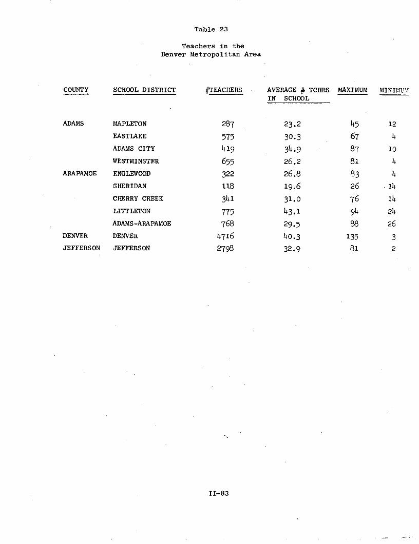
Table 23

Teachers in the

Denver Metropolitan Area

COUNTY SCHOOL DISTRICT #TEACHERS AVERAGE # TCHRS MAXIMUM MINIMUMIN SCHOOL

ADAMS MAPLETON 287 23.2 45 12

EASTLAKE 575 30.3 67 4ADAMS CITY 419 34.9 87 10

WESTMINSTER 655 26.2 81 4

ARAPAMOE ENGLEWOOD 322 26.8 83 4

SHERIDAN 118 19.6 26 14

CHERRY CREEK 341 31.0 76 14

LITTLETON 775 43.1 94 24

ADAMS-ARAPAMOE 768 29.5 88 26

DENVER DENVER 4716 40.3 135 3JEFFERSON JEFFERSON 2798 32.9 81 2

II-83

Case 5: Doctors in the State of Colorado.

To extend and generalize our previous results, the number of

doctors in each place was plotted (Fig. 7) against the population of

the place, for the entire state of Colorado.

Several features of this figure are interesting. First, if a

rough line were drawn through the data points, its slope would be

greater than unity. This indicates a positive exponential relation-

ship between doctors and city size; as population increases, the number

of doctors per thousand people generally increases. At the bottom

of the figure, however, major exceptions are shown to this rule. As

noted, the cities of large size which have less than three doctors are

all suburbs of central cities. Another interesting, although expected,

characteristic is the large scatter of doctor populations for smaller

places.

Table 24 amplifies the point that many cities, even of substantial

size, do not have local doctors. For example, even in 25,000 to 50,000

category, only 6 of the 7 cities have doctors. As noted in the DMA

case study, several large cities have only one or two doctors. For

places with less than 1000 people, 75% do not have any doctors. The

data indicate that few of these places are suburban regions of metropolitan

areas, so the lack of service is real.

II-84

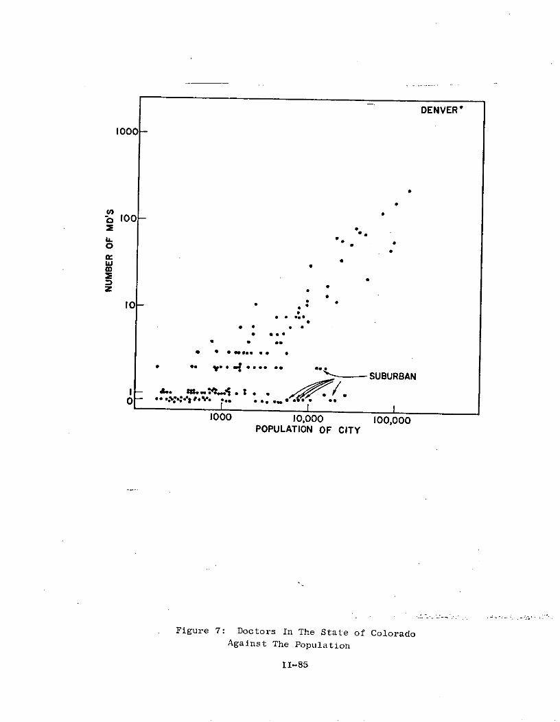
DENVER*

1000

0

0 0

z 010

O **

or

000 0,000 00,000

* * *.-

II-85

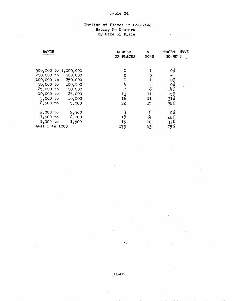
Table 24

Portion of Places in ColoradoHaving No Doctorsby Size.of Place

RANGE NUMBER W PERCENT HAVEOF PLACES MO' S NO MD'S

500,000 to 1,000,000 1 1 0%250,000 to 500,000 0 0 -100,000 to 250,000 1 1 0%50,000 to 100o,000 4 4 025,000 to 50,000 7 6 14%10,000 to 25,000 13 11 15%5,000 to 10,000 16 11 31%2,500 to 5,000 22 15 32%

2,000 to 2,500 8 8 0%1,500 to 2,000 18 14 22%1,000 to 1,500 15 10 33%

Less Than 1000 173 43 75%

II-86

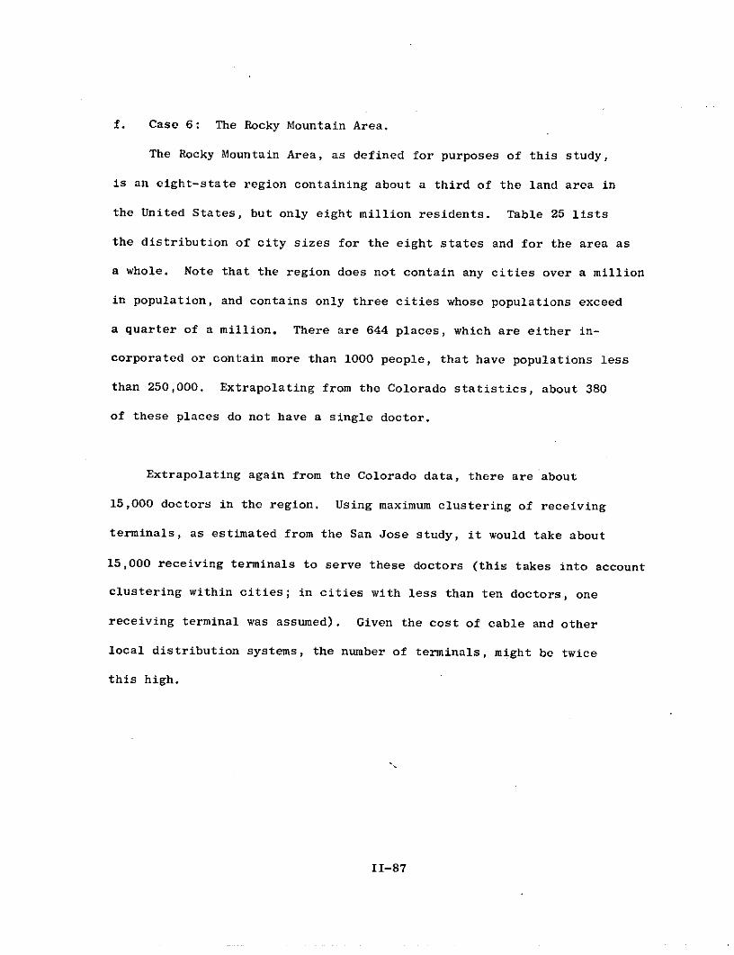
f. Case 6: The Rocky Mountain Area.

The Rocky Mountain Area, as defined for purposes of this study,

is an eight-state region containing about a third of the land area in

the United States, but only eight million residents. Table 25 lists

the distribution of city sizes for the eight states and for the area as

a whole. Note that the region does not contain any cities over a million

in population, and contains only three cities whose populations exceed

a quarter of a million. There are 644 places, which are either in-

corporated or contain more than 1000 people, that have populations less

than 250,000. Extrapolating from the Colorado statistics, about 380

of these places do not have a single doctor.

Extrapolating again from the Colorado data, there are about

15,000 doctors in the region. Using maximum clustering of receiving

terminals, as estimated from the San Jose study, it would take about

15,000 receiving terminals to serve these doctors (this takes into account

clustering within cities; in cities with less than ten doctors, one

receiving terminal was assumed). Given the cost of cable and other

local distribution systems, the number of terminals, might be twice

this high.

II-87

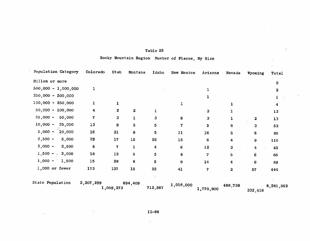
Table 25

Rocky Mountain Region Number of Places, By Size

Population Category Colorado Utah Montana Idaho New Mexico Arizona Nevada Wyoming Total

Millon or more 0

500,000 - 1,000,000 1 1 2

250,000 - 500,000 1 1

100,000 - 250,000 1 1 1 1 .4

50,000 - 100,000 4 2 2 1 3 1 13

25,000 - 50,000 7 3 1 3 6 3 1 2 13

10,000 - 25,000 13 9 5 5 7 5 6 3 53

5,000 - 10,000 16 21 9 5 11 16 5 6 89

2,500 - 5,000 22 17 15 22 15 6 4 9 110

2,000 - 2,500 8 7 1 4 6 12 3 4 45

1,500 - . 2,000 18 12 5 5 8 7 5 6 66

1,000 - 1,500 15 28 8 5 9 14 4 6 89

1,000 or fewer 173 127 15 22 41 7 2 57 444

State Population 2,207,259 694,409 1,016,000 488,738 8,281,5621,059,273 712,567 1,770,900 332,416

II-88

g. Summary

The demographic data gathered for this study documented some

common sense notions about user distributions, but it also produced

some surprises, which bear further study. As expected, substantial and

complex clustering of professionals was found. The extent of the

clustering, however, was somewhat higher than expected. In addition,

the distribution of doctors within metropolitan regions and within

cities produces substantial surprises. In general, these sections

demonstrated the need for attention to demographic detail in the design

and costing of telecommunication systems and for segmenting markets

on the basis of demographic differences.

The demographic study also provided estimates for the number of

receivers needed to serve given teleconferencing markets, focusing

primarily on doctors. More precisely, the geographical clustering

was translated into number of terminals from preliminary estimates of

cable and other costs. In the future, such demographic information

should be refined and automated, although elaborate demographic

information cannot be justified until the actual design of systems,

because of data processing costs.

II-89

D. A Methodology For Demand Assessment

While the above sections established some limits to the potential

markets for teleconferencing, before embarking on large scale implementa-

tion of services a more complete analysis must be completed. The method-

ology proposed in this section is of the level of complexity that is appro-

priate for such an analysis. The information needs are identified and

in most cases methods to acquire the information are described. Subse-

quent analyses of specific teleconferencing services should seek informa-

tion of the detail indicated by the model. Furthermore, in reviewing up-

coming experiments in teleconferencing, this or a similar model should

be used to ensure that the experiments are designed to acquire the needed

information.

1. Characteristics and Assumptions of the Study

There is a need to specify what we mean by the term "market."

Within the teleconferencing industry, we will not deal with competition

between firms in the supply of teleconferencing services. As far as the

study is concerned, there may be only one agency operating to provide the

services with teleconferencing.

However, the term market (and hence the system) incorporates more than

just the teleconferencing industry. In this analysis, one way in which

we segment the market is by dividing it into the various professional

groups within the market (see Table 26). For each occupation in the mar-

ket there will be various services which would be suited to the needs of

that occupation. While the members of the occupational class could con-

ceivably get these services with teleconferencing, there would also be

other means of satisfying their needs, such as professional journals,

II-90

Table 26

Occupational Classifications (Bureau of Census)

Classification Symboli

Professional, Technical, and Kindred:

Elementary and secondary teachers c

Engineers c2

Nurses (R.N.) c3

Accountants c4

College instructors (higher education) C5

Physicians (M.D., D.O.) C6

Lawyers and judges C7

Clergy c8

Physical scientists C9

Pharmacists c10

Dentists c

Designers and draftsmen c12

Technicians C

Musicians and music teachers l14

Managers, officials, and proprietors C

Clerical and kindred c16

Salesworkers C17

Craftsmen, foremen, and kindredc18

Operatives and kindred C1 9

Service workers including private households c 2 0

Farmers, farm managers, laborers and foremen c21

Laborers, except farm and mine c

II-91

professional meetings, and the telephone.

If we direct our efforts along the planes suggested in Table 26,

then for each of the occupational classes we generally find it would be

appropriate to view each market as being served by oligopolies with

differentiated products. The teleconferencing service is one of different

qualities than any of the other products in the market. Yet, there are

not really innumerable service alternatives; rather, there are only a few

serious alternatives in each case.

This assumed view has several implications:

The price of any service in the market depends to someextent on the price of other services in the market.

The demand for any service in the market depends to someextent on the demand for other services in the market.

There will be fairly modest price differentials in the market.

The price differential depends on the success of convincingthe public as to the superiority of the product.

Competition is principally in the area of advertising andsales promotion (to create a service brand preference whichwill benefit much more than concentration on the price dif-ferential).

We note that with our description of the market, marketshare elasticity becomes synonymous with elasticity ofsubstitution.

A final point about this study is that it will be designed to be

time varying (dynamic).

2. Estimating Potential Demand

Table 26 suggests a breakdown of users by occupational classifi-

cations. A further useful breakdown is by geograpaical areas (see Table

27). Note that the geographical units are labeled al, a2 ..... The ran-

ges are only suggested ranges and could be made more or less divisible as

II-92

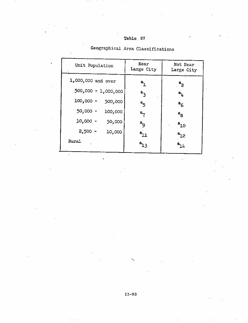
Table 27

Geographical Area Classifications

Unit Population Near Not NearLarge City Large City

1,000,000 and over a, a

500,000 - 1,000,000 a a4

100,000 - 500, 000 a5 a 6

50,000 - 100,000 a7 a8

10,000 - 50,000 a9 al0

2,500 - 10,000 al a12

Rural

II-93

resources of time and research are weighed against the additional bene-

fits of more narrowly defined ranges.

The information desired for each unit is a number and distribution

by work location, representative of the members of each occupational

classification in Table 26. It is suggested that two or three cities de-

scribed by each unit designation be studied to give an average impression

for each case.

The motivation for the collection of this data now becomes clearer.

Suppose we are studying a specific region, say either part or all of the

United States. For that region, we find how many cities are al-type

cities, how many are a2-type, and so on. We can look at our average

number of the members of each occupational classification in each city

type, and arrive at a potential demand within the region.

We have additional data which estimates the average annual growth

rate of each occupation classification over the next ten to fifteen years.

We assume that the growth rate is nearly uniform over the region. Apply-

ing this information we can now systematically describe a time varying

potential demand for teleconferencing services in the region under study.

First, let us construct a matrix, [A], whose rows (cl, c2 ,...,c )

represent the occupational classifications of Table 26. The columns of

[A] represent the geographical areas of Table 27 (al, a2:'...an). The

elements of the [A] matrix we donote as Aij

Further, let us describe the A.. as time varying quantities. For

example, we may have data which show-that the average annual growth rate

of classification ci is 5 percent. We already will have Ai. at the time

of the study, t0. Then the dynamic description cf A .. would be

II-94

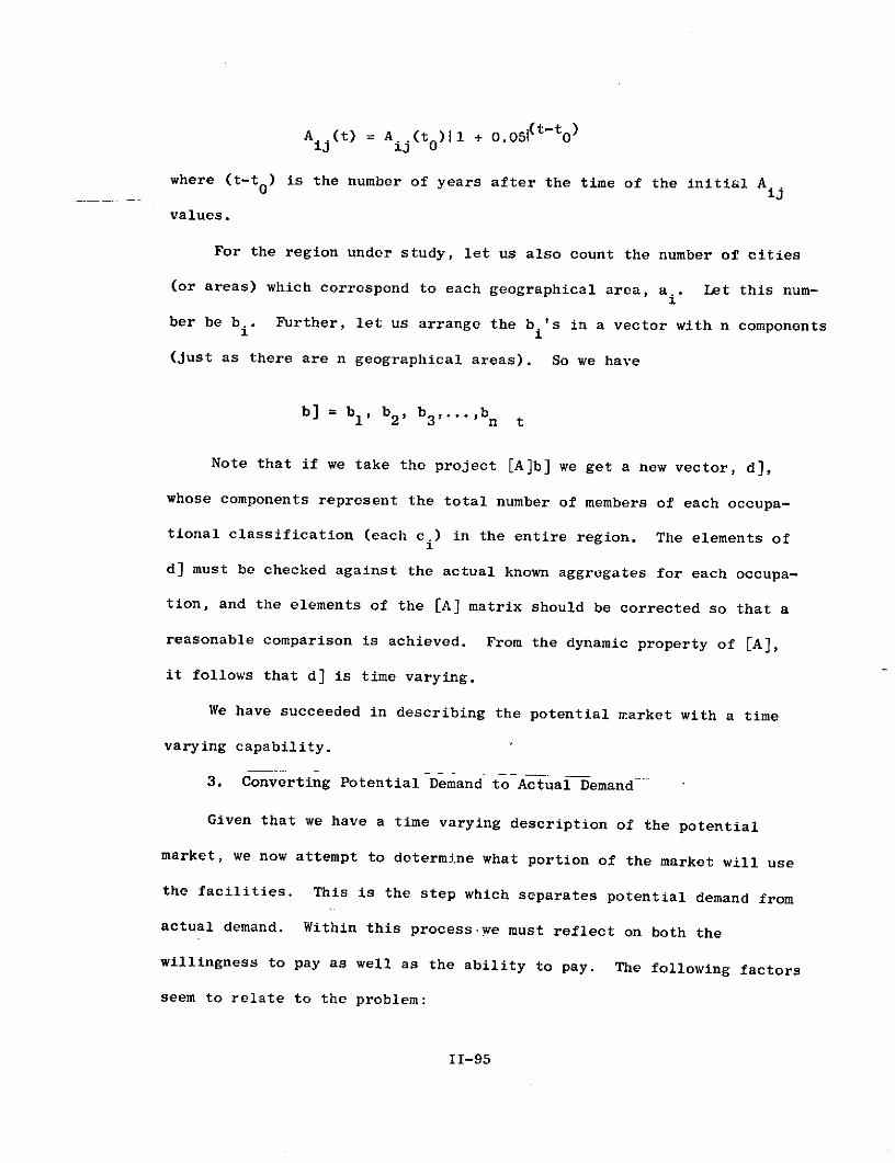
A j(t) = A.i(t )l + 0 . 0 5 1(t-t 0 )

where (t-t0 ) is the number of years after the time of the initial Aij

values.

For the region under study, let us also count the number of cities

(or areas) which correspond to each geographical area, a.. Let this num-

ber be b . Further, let us arrange the b 's in a vector with n components

(just as there are n geographical areas). So we have

b] = bl, b2 , b3 ,...,b n t

Note that if we take the project [A]b] we get a new vector, d],

whose components represent the total number of members of each occupa-

tional classification (each c.) in the entire region. The elements of1

d] must be checked against the actual known aggregates for each occupa-

tion, and the elements of the [A] matrix should be corrected so that a

reasonable comparison is achieved. From the dynamic property of [A],

it follows that d] is time varying.

We have succeeded in describing the potential market with a time

varying capability.

3. Converting Potential Demand to Actual Demand

Given that we have a time varying description of the potential

market, we now attempt to determine what portion of the market will use

the facilities. This is the step which separates potential demand from

actual demand. Within this process-we must reflect on both the

willingness to pay as well as the ability to pay. The following factors

seem to relate to the problem:

II-95

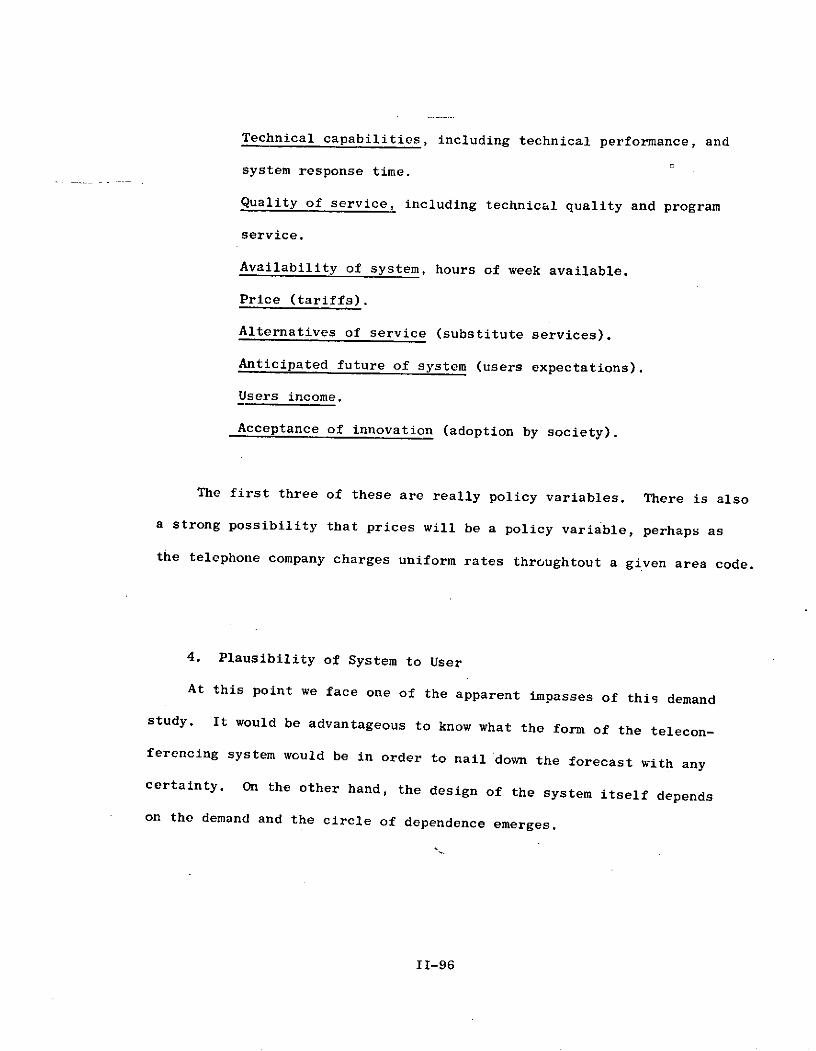
Technical capabilities, including technical performance, and

system response time. o

Quality of service, including technical quality and program

service.

Availability of system, hours of week available.

Price (tariffs).

Alternatives of service (substitute services).

Anticipated future of system (users expectations).

Users income.

Acceptance of innovation (adoption by society).

The first three of these are really policy variables. There is also

a strong possibility that prices will be a policy variable, perhaps as

the telephone company charges uniform rates throughtout a given area code.

4. Plausibility of System to User

At this point we face one of the apparent impasses of this demand

study. It would be advantageous to know what the form of the telecon-

ferencing system would be in order to nail down the forecast with any

certainty. On the other hand, the design of the system itself depends

on the demand and the circle of dependence emerges.

II-96

Ther is an important principle we should follow in this study. We

do not want to limit the policy making latitude with too narrow a study.

So we examine each A.. of the market to see what effects each system

type will have on demand. It would be appropriate to examine each Aij

and ask, "What decimal fraction of the people in the category would

plausibly employ the system under each of the two or three foremost

systems being considered?" The system design indludes technical c

capabilities, quality and availability of system service. This leads

us to two types of eliminations that can be made on the grounds of

implausibility. One is those people whose needs are not satisfied by

the technical capabilities of the system. The other is for people who

are not likely to use the system for reasons of age (too old to retrain

or follow the state-or-the-art), or possibly for other similar reasons.

The rationale is that we are trying to determine the ultimate plausible

number of users. Consider the number of people for a given A . to be

1,000. In evaluating a given system design perhaps it is determined for

the above reasons that only 800 could plausibly be served by the system

design. So we would have a system plausibility factor of 0.8 associated

with A...ij

For some alternatives we may find an extremely low factor (say, 0.05)

associated with Aij as Fij. For others we may find a very high factor,

perhpas approaching 1.0.

II-97

5. Tariffs (Pricing)*

For the purposes of the study, we are presently faced with two

specific pricing policies. One is that the price will be uniform to

all users in a given area. The second policy is that the prices depend

on the actual distribution costs to each location. For example, in a

given area a user far out from the receiving station (antenna) would

have to absorb some of the higher costs of cable installation and

maintenance to his location. Because the pricing policy is critical,

it would seem necessary to carry out the study in two independent steps,

one for each policy.

The import of the pricing policy has already been introduced in the

section on characteristics of the study. To further illustrate this, let

us suppose that a questionnaire were drafted and sent to samples of one

of the c i classifications (say lawyers and judges) in a given area. In

the questionnaire we inquired as follows:

1. What is the user's total expenditure per year on information

services?

2. Then we describe the system and the services it would provide,

noting primarily only the points interesting to the particular

class of user.

3. How much does the user spend per year on services that our system

could provide?

*See also the section on "Limitations of the Methodology."

II-98

4. What is the user's total income?

The next step would logically be to ask how many additional services

the system would provide beyond what they already receive, and to follow

this question by asking how much they would pay for the additional

services. However, we encounter two problems here:

1. We really don't know how many additional services the system

will offer, and

2. Even if we knew, the question is too abstract to receive mean-

ingful response, especially on a questionnaire.

So we now rely on the attribute of they system as a differential

product. Let the answer to question 3 above be $1,000. We will take

this figure as a competitive price. The next step is to view the

market in two parts, that which the system can supply and the second as

that which are satisfied by non-teleconferencing efforts. This division

is presumably sound because it would take an aggregated effort by the

"other"'services to match the services that the system could provide.

Consider the schedule (in Table 28) which is typical of the duopoly

with differentiated products that has now been described.

From the system designers and program costs, we should have a fairly

good idea of the cost of service to the different users of a given occupa-

II-99

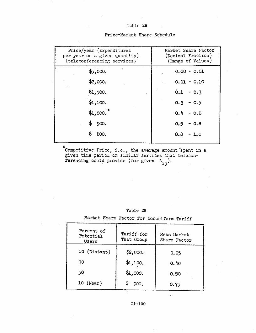
'ITable 28

Price-Market Share Schedule

Price/year (Expenditures Market Share Factorper year on a given quantity) (Decimal Fraction)(teleconferencir services) (Range of Values)

$5,000. 0.00 - 0.01

$2, 000. 0.01 - 0.10

$1,500. 0.1 - 0.3

$1,100. 0.3 - 0.5

$1,000.* 0.4 - 0.6

$ 9oo. 0.5 - 0.8

$ 600. 0.8 - 1.0

Competitive Price, i.e., the average amount'spent in agiven time period on similar services that telecon-ferencing could provide (for given Ai..).

Table 29

Market Share Factor for Nonuniform Tariff

Percent ofPotential Tariff for Mean MarketUsers That Group Share Factor

10 (Distant) $2,000. 0.05

30 $1,100. 0.40

50 $1,000. 0.50

10 (Near) $ 900. 0.75

II-100

tion within each geographical area. For example, suppose that we have

a uniform tariff of $900. Then we would estimate that our market share

factor would be between 0.5 and 0.8 of those for whom the system is a

plausible one.

If we had a nonuniform tariff rate, then we would take a weighted

average of the users in that area. This is one reason why the distribu-

tion data on users in each A.. was mentioned as important early in this

discussion. For example, suppose that for a given occupation in a given

area, we had a user distribution as in Table 29. The table illustrates

that distant users would have higher tariffs, and that the market-share

factors for them would be expected to be lower. Then the market share

factor is:

M.. = 0.1(0.05) + (0.3)(0.4) + (0.5)(0.5) + (0.1)(0.65) = 0.440.

A few additional comments seem proper about the importance of this

study. First, it may be desirable to place some type of limits on the

market share factors most likely at each price in the schedule. The

demand study is not necessarily deterministic, in the sense that an exact

demand must be forecast. The limits would be quite useful in describing

upper and lower bounds. This range of values might be more valuable

than exact.numbers whose variation is not perceived.

II-101

Another reason not to try to nail down the price differentials with

excessive accuracy is that the real effort should be directed toward

advertising and sales promotion, rather than to the exact nature of the

price differential.

The reader may recognize that this part of the analysis attempts to

relate the user's expenditures on a certain class of services to his

present expenditures. This is in recognition of the user's finite income

However, it does not presuppose that the fraction of his income spent on

these services will be necessarily constant. (The user who spend $1000

per year before may spend $1200 per year after the teleconferencing

services are introduced.) Nor does this analysis presuppose a strictly

substitute effect of the different services, for to some extent the

services may actually be complementary. On the balance, however, it

seems a priori that the substitute effect would reign predominant.

Finally, the schedule suggested would lead us to price and substitute

elasticities of demand. For all these reasons, it is suggested that a

rather intensive effort be made to determine a schedule similar to the one

presented in this section, with well-reflected ranges on the market share

factors.

II-102

6. Acceptance of Innovation*

Let us retrace our logic for a moment. First, we segmented the

market by user occupation and geographic location. This gave an upper

bound for the number of users, a base from which to work. Then we

scaled the ultimate number down to a more realistic plateau by reducing

the potential demand to only those for who the system was plausible.

We further scaled this down by a market share factor, from a market

share of demand schedule characteristic of oligopolies with differentiated

products. So now we have an idea as to the demand after the teleconferencing

systems are established and the market stabilizes.

We now turn our attention to the behavior of the market from the time

at which the teleconferencing systems are introduced until the market

stabilizes. Teleconferencing services are an innovation, and there has

been significant work done in analyzing the acceptance of innovation in

society. One such source, Diffusion of Innovations, by Everett M. Rogers,

discusses the spread of a new idea from its source of invention to its

ultimate users or adopters. This process called the adoption process has

certain characteristic phases which determine what percentage of the

ultimate user number subscribe to the innovation during the period following

its introduction.

*See also the section on "limitations of the Methodology".

II-103

One empirically suggested pattern of acceptance of an innovation over

time is an "S" shaped curve, as in Fig. 8. At first only a few pioneer

users adopt the idea, then the majority decide that the new idea is

desirable, and finally the adoption curve levels off as the influence of

the product in the market stabilizes. In our case, the plateau is esti-

mated to be the demand in the stabilized market. A similar pattern is

followed in user awareness of the product over time.

The exact shape of the adoption curve, G(t), is not known. For

one thing, the curve could rise immediately, or it could stay low for

some time rising faster at a much later time. Another unknown is the time

until stabilization which is represented by T in Fig. 8. Likely esti-

mates of T have run anywhere from an optimistic six years to a pessimis-

tic fifteen years.

We require only that the curve satisfy three criteria:

(i) G(t0 ) = 0.

(ii) It must have an S shape (suggested by empirical data).

(iii) It must have an asymptote at C = 1.0 for large values of time.

The exact form of the adoption curve does not seem to be the most

important thing. What would be more desirable would be to cover the

range of probable shapes (immediate rise to delayed rise) with a set of

calculations to get a feel for the impact of variation in shape of the

adoption curve on the demand. The time until stabilization should also

be varied in the model to see how it affects the demand. The experiences

of other prcducts can be used to see how the confidence and expectations

II-104

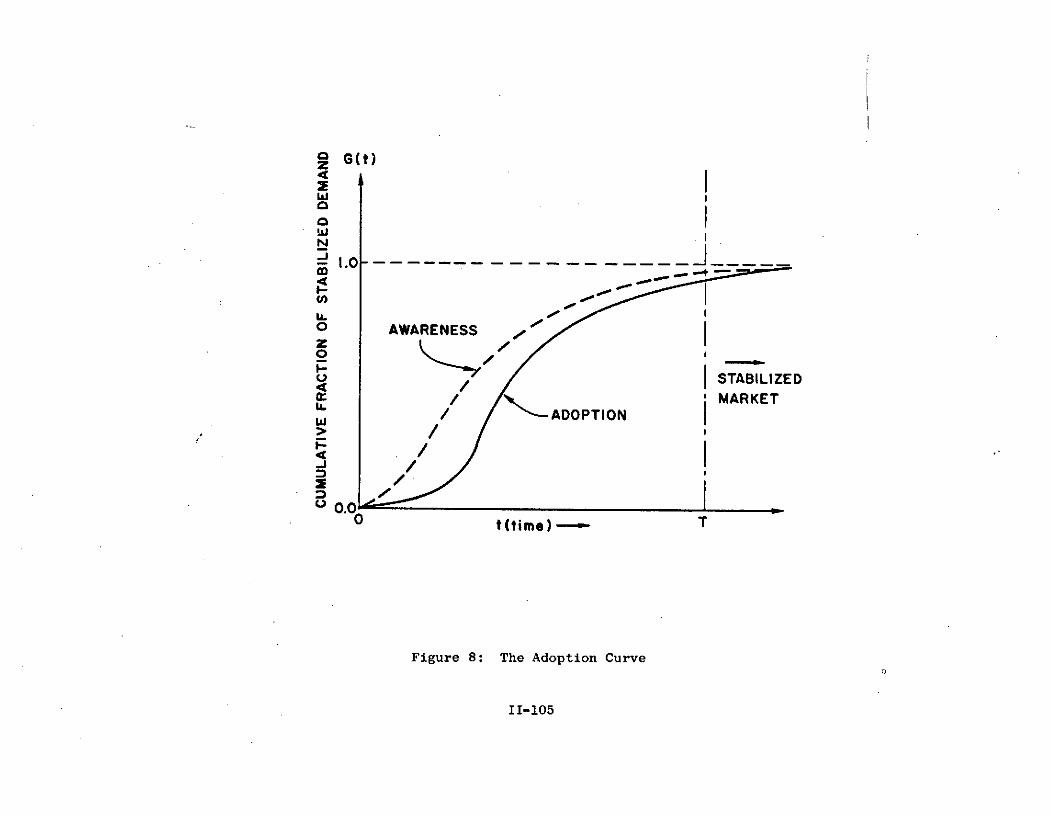
SG(t)4

w

o IN- . I

0 AWARENESS J

0.00-- I---c I STABILIZED: ' MARKET

wS/

0 t(time) - - T

Figure 8: The Adoption Curve

II-105

calculations to get a feel for the impact of variation in shape of the

adoption curve on the demand. The time until stabilization should also

be varied in the model to see how it affects the demand. The experiences

of other products can be used to see how the confidence and expectations

of users have manifested themselves in the past.

Further thought is necessary regarding whether any particular

adoption curve will be appropriate for all segments of the market, or

whether individual curves will be needed for each row, column, or element

of the [A].

II-106

7. Putting It All Together--Demand

For a given system design

For a given tariff policy

For a given region

Assuming one G(t) (adoption curve) for the whole region.

The demand is described as

(M1,1)(F,)A1,1(t) ......... (M, n (F,n)A ,n(t) b

(M ,1)(F 2,1)A 2,1(t) ...... (M 2.n)(F 2,n)A ,n (t) b2

D(t)] = G(t)

(M )(F )A (t) ...... (M )(F )A (t) bm,l m,l m,l m,n m,n m,n n

where D(t)] is the vector each of whose components represent the expected

actual demand by people in each occupation at time t.

G(t) is the adoption curve.

M.. is the market share factor.

F.. i is the plausibility factor.

A is the potential demand.

b] is the vector whose components represent the number of cities

of each type in the region.

II-107

If we had reason to have a different G(t) for each occupation, then

the matrix would be pre-multiplied by a row vector G(t), each of whose

m elements would apply to the corresponding occupational classification

(i.e., Gi(t) corresponds to ci, the it h row of the [A] matrix).

Finally, although for conceptual reasons we have considered the

Mij and the Fij factors separately, there is no reason why they cannot

be combined into one factor in practice, as long as that one factor

retains all the properties of the original factors.

11-108

8. Example Calculation: Determinations of Price and SubstituteElasticities of Demand

C

Using the price-market share schedule displayed in the description

of market share factors earlier, we proceed with the following example:

A particular A.. is being considered.

A uniform tariff policy is followed.

We assume that a 95% level of the adoption curve is to be reached

in four years. (Other adoption curve characteristics previously

indicated are also to be followed.)

The occupational classification, ci, grows at five percent

per year.

We assume a system palusibility factor of 0.8 associated with

A...j

We assume a uniform distribution on the M.. over the ranges

shown.

There are 1,000 people in Aij at t .

We have from the above the following time-varying description of A i:

A..(t) = 1,0 0 0 (1 .05 )t-tO1j

We also construct an adoption curve which meets all the specifications

desired. This could be done by a table of G(t) vs t in years, or by some

continuous function. We opt for the latter:

-t1- e

G(t) = , t 0,1 + e

II-109

whose characteristics are:

(i) G(O) = 0.

(ii) Asymptote at G = 1.0.

(iii) "S" shaped curve (see Fig. 9).

(iv) G(4) = 0.96, or in 4 years we achieve the 95% adoption rate.

We now make calculations for the values of A.. and G.i in years one

through four, shown in Table 30, and follow with the demand calculations

in Table 31.

Table 30

Example Values for A..(t) and G..(t)

t A..(t) G..(t)

1 1,050 0.45

2 1,103 0.77

3 1,157 0.91

4 1,216 0.96

II-110

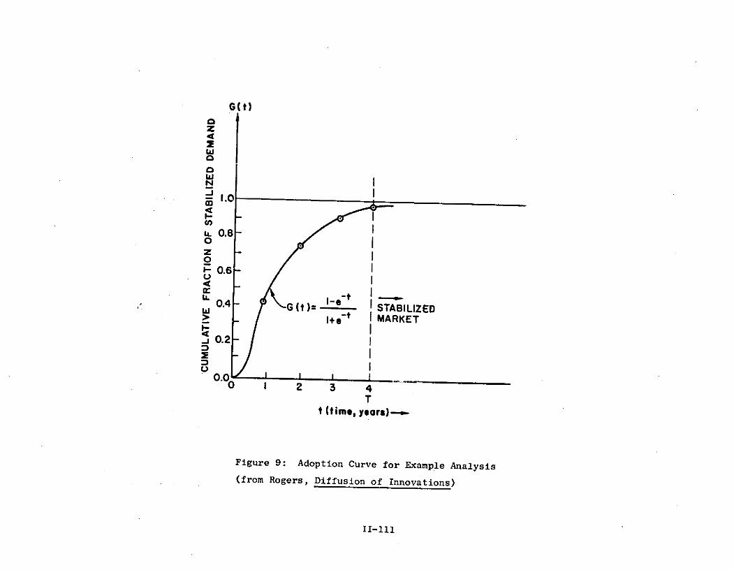
G(t)

4

w

N- 1.0

0

i.

I-

z

1 0.6 -

20.2

0.00 I 2 3 4

t (time, years)--@

Figure 9: Adoption Curve for Example Analysis

(from Rogers, Diffusion of Innovations)

II-lll

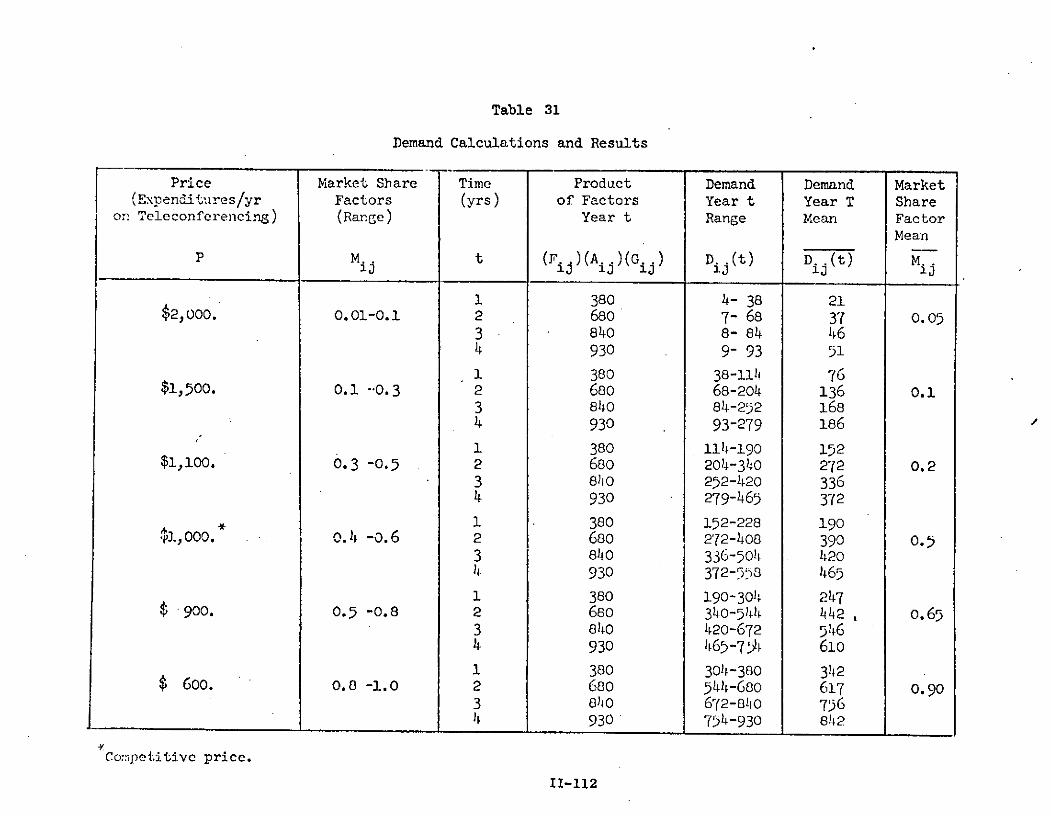
Table 31

Demand Calculations and Results

Price Market Share Time Product Demand Demand Market(Expenditures/yr Factors (yrs) of Factors Year t Year T Share

on Teleconferencing) (Range) Year t Range Mean FactorMean

P M ijt (F. )(Aj)(G ) D.. (t) D. (t) M..

1 380 4- 38 21$2,000. 0.01-0.1 2 680 7- 68 37 0.05

3 840 8- 84 464 930 9- 93 51

1 380 38-11, 76$1, 500. 0.1 -.0.3 2 680 68-204 136 0.1

3 840 84-252 1684 930 93-279 186

1 380 114-190 152$1,100. 0.3 -0.5 2 680 204-340 272 0.2

3 840 252-420 3364 930 279-465 372

1 380 152-228 190T1 , 000. -0.6 2 680 272-408 390 0.5

3 840 336-504 4204 930 372-558 465

1 380 190-304 247$ 900. 0.5 -0.8 2 680 340-544 442 , o.65

3 840 420-672 5464 930 465-7 4 610

1 380 304-380 342$ 600. 0.8 -1.0 2 680 544-680 617 0.90

3 840 672-840 756I4 930 754-930 842

Competitive price.

11-112

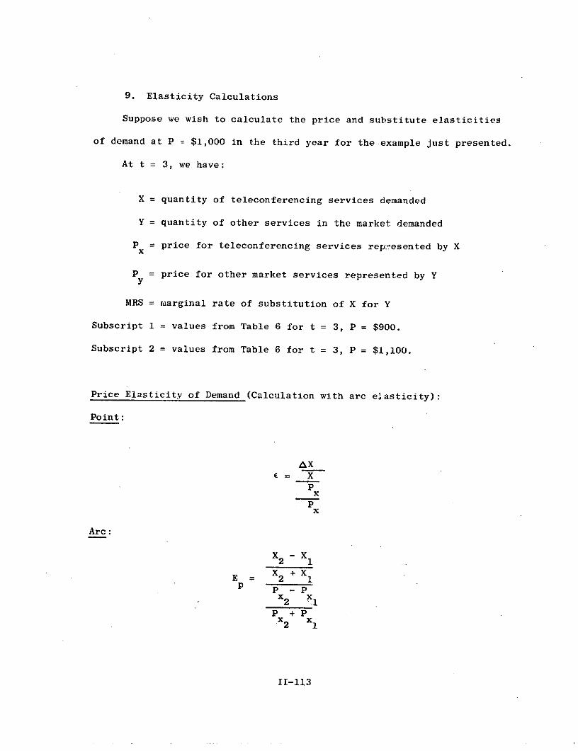
9. Elasticity Calculations

Suppose we wish to calculate the price and substitute elasticities

of demand at P = $1,000 in the third year for the example just presented.

At t = 3, we have:

X = quantity of teleconferencing services demanded

Y = quantity of other services in the market demanded

P = price for teleconferencing services rep:resented by X

P = price for other market services represented by Yy

MRS = marginal rate of substitution of X for Y

Subscript 1 = values from Table 6 for t = 3, P = $900.

Subscript 2 = values from Table 6 for t = 3, P = $1,100.

Price Elasticity of Demand (Calculation with arc e.asticity):

Point:

AXE= X

Px

Px

Arc:

X2 1

E = X2 + X1S P - P

x x2 -1P +Px2 x

II-113

= 336 - 546E = 336 + 546 = -2.4

p 1100 - 900

1100 + 900

Substitute Elasticity of Demand (Calculation with arc elasticity):

Point:

A(X/Y) A(X/Y)t = X/Y = X/Y

AMRS A(P /P )x yMRS

P /Px y

Arc:

(X/Y)2 - (X/Y)1

E = (X/Y)2 + (X/Y)1S(P /P ) - (P /P )x y2 x y 1

(P /P ) + (P /P )x y2 x yl

= 0.4 - 0.65E = 0.4 + 0.65 = -2.4

1.1 - 0.9

1.1 + 0.9

Further work was done in an attempt to relate income elasticity of

demand to the two elasticities already described; however, a realistic

relationship would require data of a much more abstract nature. By this

we refer to the fundamental equation of price theory, the Slutsky equation,

which relates the three types of elasticity. However, in the case presented

with this project, information regarding changes in the marginal rates of

II-114

substitution of the information services is required along iso-utility

lines (in the microeconomic sense). This data is not easily obtained.

The.result of the procedure above is that we would now have the

price and substitution elasticities associated with each A... With these

matrices, we can attempt to predict the impact on the change in demand

for teleconferencing services in any occupation/geographic area due to

changing the prices of the services or the demand for substitute services.

The extension of the impact to the entire region follows in the same way

the overall demand was projected from the information associated with the

elemenis of the [A] matrix.

II-115

PRECEDING PAGE BLANK NOT FIME

10. Limitations of the Methodology

There are three general areas in which significant limitations of

the methodology suggested are found. The first is in the adoption curve

concept. It has been suggested frequently that the adoption curve rises

in an "S" shaped curve to a plateau, an asymptote as time gets large.

However, some sources contend that after the adoption curve reaches its

peak and holds for some time, it declines exponentially to another

plateau. For example, the telegraph reached a peak as it was adopted,

but because of new services, its use actually has declined to some extent

since it peaked.

This does not deal a fatal blow to the methodology which has here

been proposed. In the section on adoption curves, it was mentioned that

further thought on the shape of the curve is necessary. It is difficult

to imagine what services would cause the adoption curve for teleconferencing

services to decline as it did for the telegraph; however, it would have

most likely been hard for those developing the telegraph to see how the

adoption curve for that great innovation to peak out and then decline.

In this fast moving age of technology, we should not blind ourselves to

the idea that a smilar behavior is likely to befall the adoption curve

for teleconferencing services.

The second area of concern is in the uncertainty associated with

certain variables. In the price-market share schedule (see Table 3),

II-117

there was a range of market share factors associated with each price.

The example assumed a uniform probability distribution of the values

within the range used. However, the actual study suggested in this

methodology might reveal a different distribution. The calculations

would then be based on that distribution.

Similarly, the value of T in the adoption curve, representing the

time until market stabilization, might be described by a probablilty

distribution instead of straightforward case studies ba;3ed on various

values of T.

Another uncertainty is the location of the "S" in the adoption

curve. This can be studied with probabilistic analysis, or in a case

study given various locations of the curve.

This methodology has first suggested the case studies of these

variables to see which ones are sensitive enough to warrant further

investigation of the probabilistic nature just described. In any event,

analysis with distributions represent extensions of this methodology, and

would not deem any of the suggested output of the study invalid.

The third area of concern again deals directly with the price-

market share factor schedule, such as that of Table 3. We have proceeded

in this study under the assumption that the services provided by the

II-118

teleconferencing industry are introduced into a market which presently

exhibits a high degree of stability among the already existent services

(such as professional journals, telephone service, professional meetings,

etc). The market share factors are based on the characteristics of the

oligopoly with differential products, and the "competitive price" in the

schedule, as well as the price of the services provided by the tele-

conferencing industry, are likely to vary. Let us consider these varia-

tions one at a time.

We arrived at the competitive price by determining how much the

user of market services presently (before the teleconferencing services

are introduced) spends with a given time period, say, a year. It is

realized that after the teleconferencing services are introduced, the

user may actually increase his total expenditure on services provided by

the market, because of the introduction of the teleconferenicing services,

the market share factors originally assigned will not change. All the

demand and elasticity calculations will remian valid, for the effective

competitive price will not change.

However, if one of the substitute services comes forth with a drastic

price change, then two consequences emerge.

1. The "competitive price" is altered significantly, and the price-

market share schedule must be'adjusted accordingly.

II-119

2. The impact of the price change on demand can no longer be

accurately predicted since the elasticity is a concept dependent

on changes "in the limit" (as the price change is fairly small).

New elasticities based on the new price-market share schedule

must be derived, using the same procedure described in the

section on elasticities.

The second consideration is what happens when the price of telecon-

ferencing services is changed. The pricing has been viewed as a policy

variable, and if the price is changed, the study will simply use the same

price-market share schedule with the new price being used instead of the

old one to determine the market share. No modificatio in the model is

required. The demand is described with one set of M.. before the change,

and a new set of M.. afterwards.II120

11-120

E. REFERENCES

1. LICKLIDER, J. C. R., "A Crux in Scientific and Technical Communica-tion," Am. Psychologist, 21, 11, (Nov. 66), p. 1044.

2. SCHUSSEL, G., Data Management, 7, 24, (1969), referenced in Schneider,John H., Selective Dissemination and Indexing of ScientificInformation," Science, 173, p. 301.

3. GARVEY, WILLIAM D.; LIN, NAN; AND NELSON, CARNOT E., "Communicationin the Physical and the Social Sciences," Science, (11 Dec. 1970),70, p. 1168.

4. LIEBESNEY, F., "Lost Information: Unpublished Conference Papers,"Proc. Internat. Conf. on Sci. Info., Washington, D.C., Nas, (1959),pp. 475-480, referenced in Paisley, William J. and Paisley,Matilda B.," Communication at Scientific and Professional Meetings,Stanford University, Stanford, Ca., (April 1971), p. 1-3.

5. PAISLEY. WILLIAM J., AND PAISLEY, MATILDA B., Communication atScientific and Professional Meetings, Stanford University, Stanford,Ca., (April 1970), p. 2-1.

6. PAISLEY and PAISLEY, Op. Cit., p. 2-7.

7. AMERICAN PSYCHOLOGICAL ASSOCIATION, Project on Scientific InformationExchange in Psychology, APA-PSIEP Report No. 16, (1966).

8. SCHNEIDER, JOHN H., "Selective Dissemination and Indexing of ScientificInformation, Science, 173.

9. PARKER, EDWIN B., "Behavioral Research in the Development of aComputer-Based Information System," in Nelson, Carnot E., andPollock, Donald K., Communication Among Scientists and Engineers,Heath Lexington Books, Lexington, Mass., (1970), p. 285.

10. RUBENSTEIN, ALBERT, et. al., "Explorations on the Information SeekingStyle of Researchers," Carnot and Nelson, Op. Cit., pp. 209-232.

11. PRICE, DEREK J. de S., Little Science, Big Science, Columbia UniversityPress, N.Y., 1963.

12. LANCASTER, F. WILFRED; and GILLESPIE, CONSTANTINE J., "Design andEvaluation of Information Systems," Ann. Rev. of Info. Sci.and Tech., Vol. 5., Encyclopedia Britannica, Inc., Chi, Ill.,(1970).

13. MATTHEWS, F. W., Proc. Am. Soc. Info. Sci., 7, (1970), p. 315,referenced in Schneider, Science, Op. Cit.

11-121

14. BUCHANNAN, J.R. and KIDD, E.M., "Development of a Computer SystemWith Console Capability," for Neuc. Safety Info. Center.,A.S.I.S. Annual Meeting, San Francisco, 1-4 October 1969,Proc. Vol 6., p. 151-158., referenced in Lancaster andGillespie, Op. Cit.

15. ORR, RICHARD H., "The Scientist As an Information Processor: AConceptual Model Illustrated With Data On Variables Relatedto Library Utilization," Nelson and Pollcck, Op. Cit.

16. PAISLEY, WILLIAM J., The Flow of (Behavioral) Science Information:A Review of the Current Literature, Institute for CommunicationResearch, Stanford University, Stanford, California, (1965).

17. ALLEN, THOMAS J. and GERSTEBERGER, PETER G., Criteria for theSelection of an Information Source, Working Paper No. 284-67Alfred P. Sloane School of Management, Massa chusetts Instituteof Technology, Cambridge, Massachusetts, (1968).

18. ROSENBERG, R. V., The Application of Psychometric Techniques toDetermine the Attitudes of Individuals T gward InformationSeeking, Bethlahem, Penn., Leigh Univ. Center for theInformation Sciences, Rept. No. 2, (1966).

19. RUBENSTEIN, ALBERT H., et. al., Op. Cit.

20. O'GARA, P. W., Physical Location as a Determinant of the Possibilityamong R and D Engineers, S. MI. Thesis, Alfred P. Sloane Schoolof Management, MIT, Cambridge, Mass., (1968), referenced inAllen, "Information Needs and Uses," Vol. 4, Annual Reviewsof Information Science and Technology, Encyclopedia Britannica,Inc., Chicago, Ill., (1969).

21. ALLEN, Ann. Rev. of Info. Sci. and Tech., Op. Cit.

22. PANKO, RAYMOND R., Political Aspects of Interdepartmental Communication:A Career Capitalization Model, M.B.A. Thesis, Seattle University,Wa., (1971).

23. FROHMAN, Determinants of Library Use in an Industrial Firm, Term PaperMIT, (1968), referenced in Allen, Ann. Rev. Info. Sci. and Tech.,Op. Cit.

24. ACKOFF, R. L. and Halbert, M. H., An Operations Research Study ofThe Scientific Activity of Chemists, Case Inst. of Tech., Cleveland.

25. SHAW, R. R., Pilot Study on the Use of Scientific Literature byScientists, NSF, Washington, D. C., (1956).

II-122

26 MELTZER L., Scientific Productivity in Organizational Settings",Jour. Sc. Issues, 2, (1956), pp. 32-41.27. PELZ, DONALD C. and ANDREWS,NProductive Cites for Research an Development, Wiley

28. SCHILLING, C. W., BERNARD28. SCHILLING, C. W, BERNA RD, and TYSON, J.W., Informal CommunicationAmong Bioscientist Geo. Wash. Univ., Biologca SciencesCommunication Project, Wash., D. C. (1964).gical

29. ALLEN, THOMAS J., ADRIEN, M. and GERSTENFIELD, A. Time AllocationAmong Three Technical Information Channels ByRanEnginee. Alfre Sloane School of Management, WorkingPaper No. 184-66, MIT, Cambridge, Mass., (1966).30. PARKER, EDWIN B., and PAISLEy, WILLIAM j., "Resarch for Psychologistsat the Interface of the Scientist and His Information System,Am. Psychologist, 21, 11, (November 1966).31. WENTE, VAN A. and YOUNG, GIFFORD A., "Current Awareness andDissemination in ACS Report Rates Information System Efficiency,Chem. & Engr. News, 47, 31, (July 1969), pp. 45-46.32. MOHARDT, FOSTER E. and OLIVERI, BLANCH L., A National Network ofBiological-Agricultural

Libraries," Coll. & Res. Libs.,(January 1967), p. 9. Res

33. FEDERATION INTERNATIONALE de DOCUMENTACION,

Abstract Services,Vol. 1, FID Publication No. 455, The Hague, Netherlands(1969), in Scheneider, Science, Op. Cit.34. NATIONAL ACADAMV OF SCIENCE/NATIONAL ACADAMy OF ENGINEERS, Committeeonsientific and Technical Communication Report, NAS,Washington D. C., (1969), p. 157.

35. SCHNEIDER, Science, Op. Cit.

36. NAS/NAE, Op. Cit.

37. BUSH, VANNEVAR, "As We May Think," Th Atlantic Monthly (J 19PP. 1017108. he Alantic y, (July 1945)38. CHU, W. N., "Optimal File Allocation in a Multiple Computer System,"IEEE Transactions on Computers, C-18:10, (October 1969) pp. 885-889, referenced in Simms and Fchs, Communcations Technology,Ann. Rev. of Info. Sci. and Tech., Vol. 5, (1970) EncylopediaBritannica, Inc., Chi. Il1.

II-123

39. SIMS, WILLIAM E., "Preview of 1979: Communications and the Computer,"J. Data Mgt., 7, 9, (September 1969), pp. 20-23., referencedin Teplitz, Arthur, "Microfilm and Reprography," Ann. Rev. ofInfo. Sci. and Tech., Vol. 5, (1970), Encyclopedia Britannica,Inc., Chi., Ill.

40. The Medical Media Network is operated by the extension service ofUCLA. Videotapes and Films are produced with the cooperationof several medical institutions of California. MMN offers ayear-long program of continuing education fro doctors andnurses.

41. These services are covered in the University of Wisconsin report,issused in conjunction with this project.

42. PARKER, EDWIN B., "Systems Theory Analysis of Feedback Mechanismsfor Information systems," Federacion International deDocumentacion, Congreso Internacional de Documentacion,Buenos Aires 21-24 September 1970, Proceedings I. a. 12.

43. Why Health Security, Health Security program, Committee for NationalHealth Insurance, 806 15th St., N.W., Washignton, D.C., 20025,July 1970.

44. "Health Care: Supply, Demand and Politics," Time Magazine, June 7, 1971.

45. DeLand, E.C. and Waxman, B.D., Review of Hospital InformationSystems, Rand Corporation, June 1970. To be included as partof the Handbook of Biomedical Information Systems, EncyclopediaBritannica, Inc., Chicago. p.2.

46. "Closed Television Circuit Links Two Hospitals," TelecommunicationJournal, Vol. 38-111/1971, (pp. 131-132), p. 132.

47. Ibid.

48. Medical Media Network is operated by the University Extension of UCLA.Films and videotapes are offered in a year-long package ofcontinuing education for doctors and nurses.

49. DOYLE, FRANK J. and GOODWILL, DANIEL Z., An Exploration of the Futureof Medical Technology, Bell Canada, March 1971.

50. AMERICAN MED ASS., Directory of Physicians, 1969.

51. U.S. Bureau of the Census, Preliminary Reports from the 1970 Census.Series PCI - BC3.

II-124

Chapter III

A. Introduction

The purpose of this chapter is to discuss the economic characteris-

tics of a satellite communication ground station. It presents the costs

of the ground station antenna and pre-amplifier and derives the relation

between G/T and minimum cost. Also the cost of the transmitter and of

certain miscellaneous items are described. The results of this cost eval-

uation are used to obtain numerical approximations of a least-cost

satellite system, including both ground segment and satellite segment,

as described in Chapter V of this report.

III-1

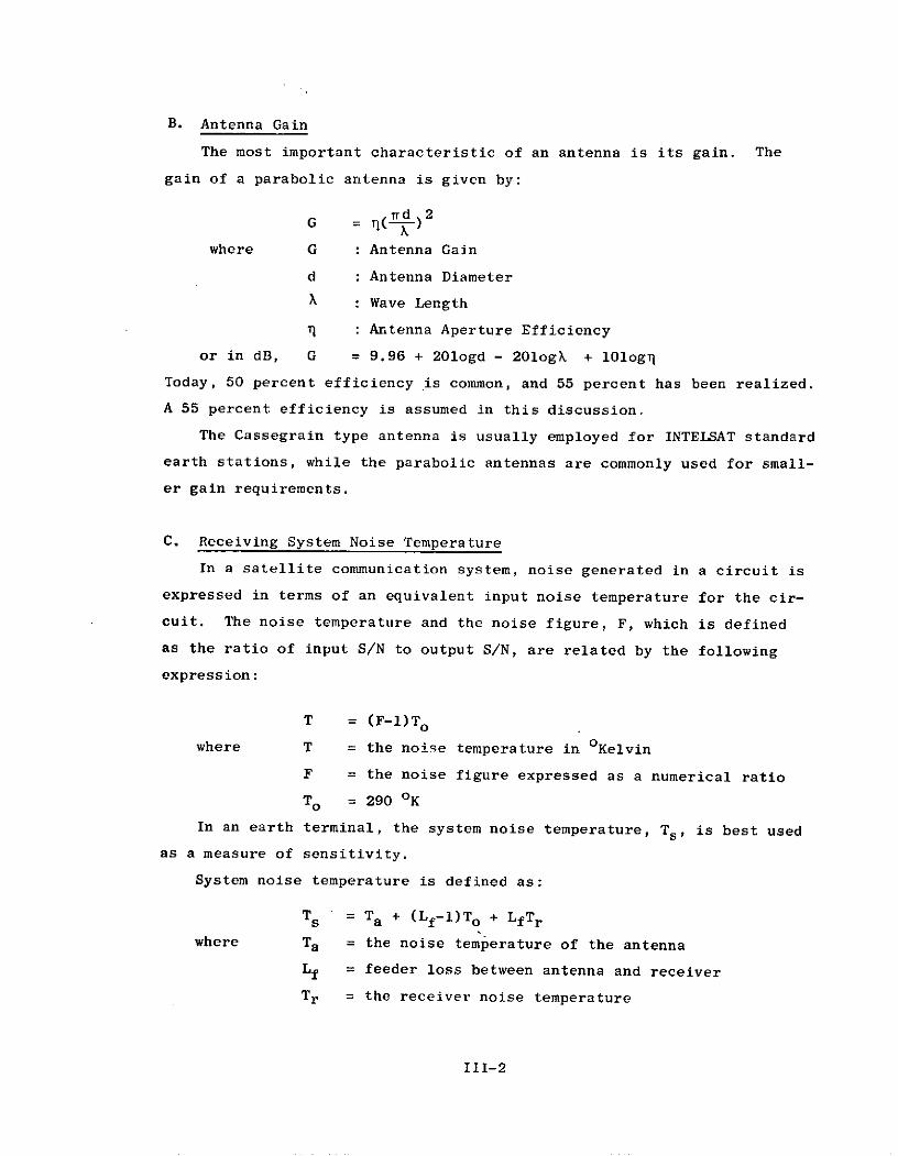
B. Antenna Gain

The most important characteristic of an antenna is its gain. The

gain of a parabolic antenna is given by:

G = )q( 2

where G : Antenna Gain

d : Antenna Diameter

X : Wave Length

T : Antenna Aperture Efficiency

or in dB, G = 9.96 + 20logd - 20logk + 10logy

Today, 50 percent efficiency is common, and 55 percent has been realized.

A 55 percent efficiency is assumed in this discussion.

The Cassegrain type antenna is usually employed for INTELSAT standard

earth stations, while the parabolic antennas are commonly used for small-

er gain requirements.

C. Receiving System Noise Temperature

In a satellite communication system, noise generated in a circuit is

expressed in terms of an equivalent input noise temperature for the cir-

cuit. The noise temperature and the noise figure, F, which is defined

as the ratio of input S/N to output S/N, are related by the following

expression:

T = (F-1)To

where T = the noise temperature in oKelvin

F = the noise figure expressed as a numerical ratio

T o = 290 OK

In an earth terminal, the system noise temperature, Ts, is best used

as a measure of sensitivity.

System noise temperature is defined as:

T s = Ta + (Lf-1)T o + LfTr

where Ta = the noise temperature of the antenna

Lf = feeder loss between antenna and receiver

Tr = the receiver noise temperature

III-2

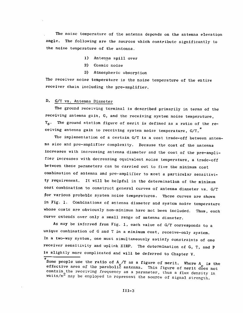
The noise temperature of the antenna depends on the antenna elevation

angle. The following are the sources which contribute significantly to

the noise temperature of the antenna.

1) Antenna spill over

2) Cosmic noise

3) Atmospheric absorption

The receiver noise temperature is the noise temperature of the entire

receiver chain including the pre-amplifier.

D. G/T vs. Antenna Diameter

The ground receiving terminal is described primarily in terms of the

receiving antenna gain, G, and the receiving system noise temperature,

Ts . The ground station figure of merit is defined as a ratio of the re-

ceiving antenna gain to receiving system noise temperature, G/T.

The implementation of a certain G/T is a cost trade-off between anten-

na size and pre-amplifier complexity. Because the cost of the antenna

increases with increasing antenna diameter and the cost of the pre-ampli-

fier increases with decreasing equivalent noise temperature, a trade-off

between these parameters can be carried out to five the minimum cost

combination of antenna and pre-amplifier to meet a particular sensitivi-

ty requirement. It will be helpful in the determination of the minimum

cost combination to construct general curves of antenna diameter vs. G/T

for various probable system noise temperatures. These curves are shown

in Fig. 1. Combinations of antenna diameter and system noise temperature

whose costs are obviously non-minimum have not been included. Thus, each

curve extends over only a small range of antenna diameter.

As may be inferred from Fig. 1, each value of G/T corresponds to a

unique combination of G and T in a minimum cost, receive-only system.

In a two-way system, one must simultaneously satisfy constraints of one

receiver sensitivity and uplink EIRP. The determination of G, T, and P

is slightly more complicated and will be deferred to Chapter V.

Some people use the ratio of A /T as a figure of merit. Where A is theeffective area of the parabolic antenna. This figure of merit does notcontain the receiving frequency as a parameter, thus a flux density inwatts/m 2 may be employed to represent the source of signal strength.

III-3

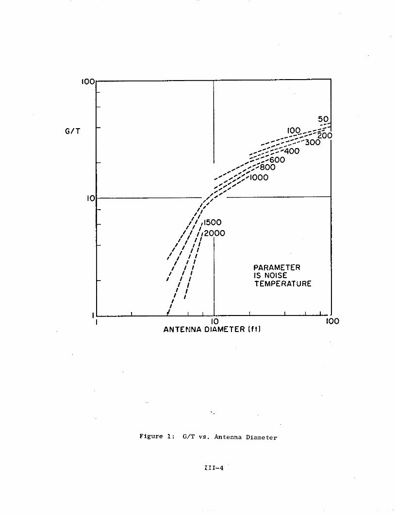
100

50G/T 100 .

00-- 300

,- - -- OO

-- 600800

S/ ,1500

// / 02000

-- -

/ /-,/I!

/ /T PARAMETER/ I IS NOISE

/ / TEMPERATURE

I

I0 100ANTENNA DIAMETER (ft)

Figure 1: G/T vs. Antenna Diameter

III-4

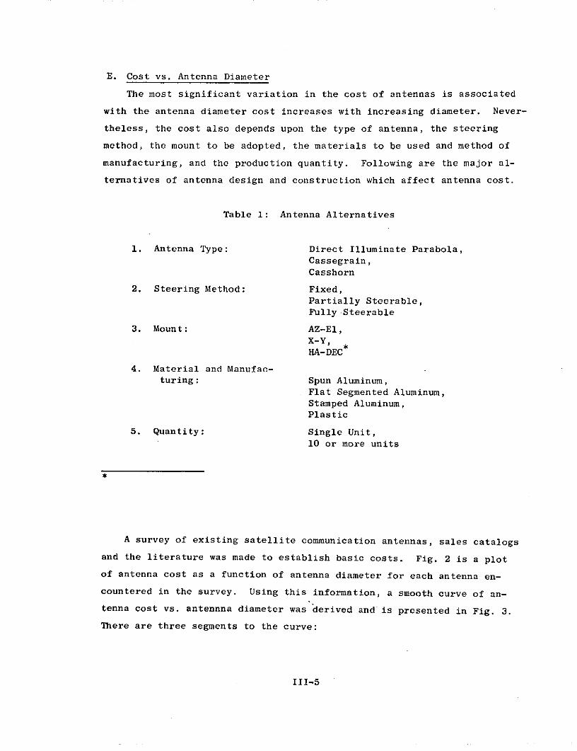
E. Cost vs. Antenna Diameter

The most significant variation in the cost of antennas is associated

with the antenna diameter cost increases with increasing diameter. Never-

theless, the cost also depends upon the type of antenna, the steering

method, the mount to be adopted, the materials to be used and method of

manufacturing, and the production quantity. Following are the major al-

ternatives of antenna design and construction which affect antenna cost.

Table 1: Antenna Alternatives

1. Antenna Type: Direct Illuminate Parabola,

Cassegrain,

Casshorn

2. Steering Method: Fixed,

Partially Steerable,

Fully Steerable

3. Mount: AZ-E1,X-Y,HA-DEC

4. Material and Manufac-

turing: Spun Aluminum,

Flat Segmented Aluminum,Stamped Aluminum,Plastic

5. Quantity: Single Unit,10 or more units

A survey of existing satellite communication antennas, sales catalogs

and the literature was made to establish basic costs. Fig. 2 is a plot

of antenna cost as a function of antenna diameter for each antenna en-

countered in the survey. Using this information, a smooth curve of an-

tenna cost vs. antennna diameter was derived and is presented in Fig. 3.

There are three segments to the curve:

III-5

IOM

M

0

0=IOOK

z

z< 010 K ---- -- -

LL IOKO

- v0 o

K 1

DIFFERENT SYMBOL* SHOWS DIFFERENT

SOURCE

I 10 100 1000ANTENNA DIAMETER (ft)

Figure 2: Cost vs. Antenna Diameter

II1-6

M

o7100K

0

zz

K

2-4 GHz

10001 10 100 .1000

ANTENNA DIAMETER (ft)

Figure 3: Cost vs. Antenna Diameter

III-7

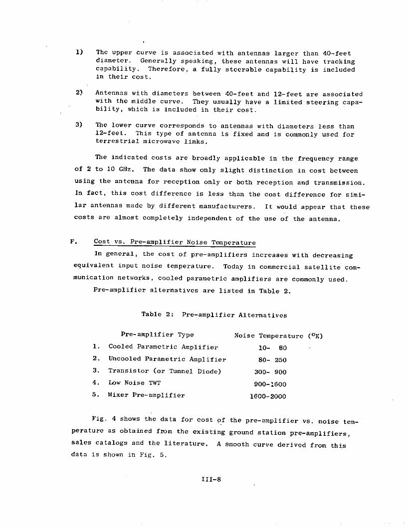
1) The upper curve is associated with antennas larger than 40-feetdiameter. Generally speaking, these antennas will have trackingcapability. Therefore, a fully steerable capability is includedin their cost.

2) Antennas with diameters between 40-feet and 12-feet are associatedwith the middle curve. They usually have a limited steering capa-bility, which is included in their cost.

3) The lower curve corresponds to antennas with diameters less than12-feet. This type of antenna is fixed and is commonly used forterrestrial microwave links.

The indicated costs are broadly applicable in the frequency range

of 2 to 10 GHz. The data show only slight distinction in cost between

using the antenna for reception only or both reception and transmission.

In fact, this cost difference is less than the cost difference for simi-

lar antennas made by different manufacturers. It would appear that these

costs are almost completely independent of the use of the antenna.

F. Cost vs. Pre-amplifier Noise Temperature

In general, the cost of pre-amplifiers increases with decreasing

equivalent input noise temperature. Today in commercial satellite com-

munication networks, cooled parametric amplifiers are commonly used.

Pre-amplifier alternatives are listed in Table 2.

Table 2: Pre-amplifier Alternatives

Pre-amplifier Type Noise Temperature (OK)

1. Cooled Parametric Amplifier 10- 80

2. Uncooled Parametric Amplifier 80- 250

3. Transistor (or Tunnel Diode) 300- 900

4. Low Noise TWT 900-1600

5. Mixer Pre-amplifier 1600-2000

Fig. 4 shows the data for cost of the pre-amplifier vs. noise tem-

perature as obtained from the existing ground station pre-amplifiers,

sales catalogs and the literature. A smooth curve derived from this

data is shown in Fig. 5.

III-8

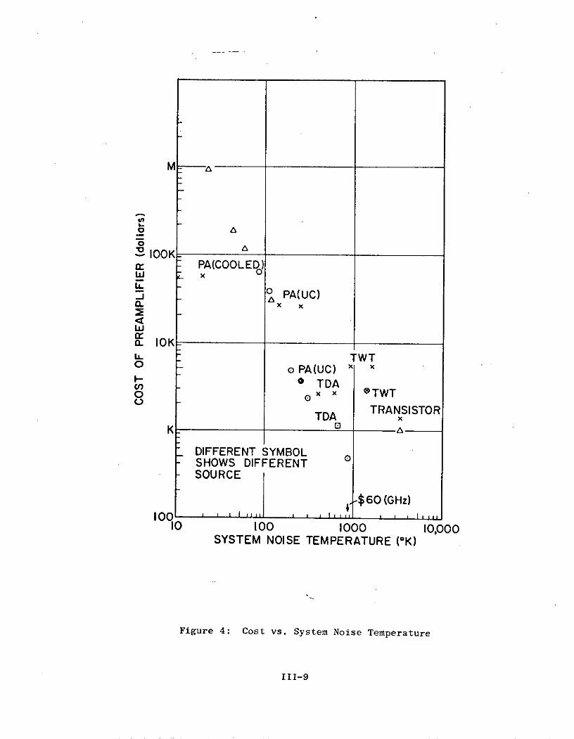
IOOK

- -PA(COOLED o )w x

SPA(UC)x x

E-

a. IOK".L TWTo o PA(UC) x

I- TDA0o x x ®TWT

TRANSISTORTDA x

DIFFERENT SYMBOLSHOWS DIFFERENTSOURCE

-$60 (GHz)100 1 , 11111

10 100 1000 10,000SYSTEM NOISE TEMPERATURE (OK)

Figure 4: Cost vs. System Noise Temperature

III-9

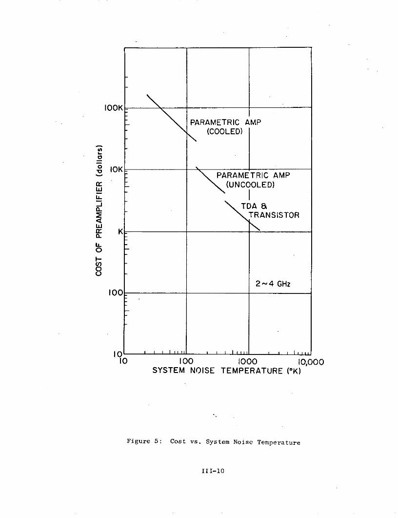
IOOK -

PARAMETRIC AMP(COOLED)

IOK-PARAMETRIC AMP

cr _(UNCOOLED)ILJ

--: \q TDA tTRANSISTOR

c- K

0 -I-

82-~ 4 GHz

100

10 i I I I10 100 1000 10,000

SYSTEM NOISE TEMPERATURE (°K)

Figure 5: Cost vs. System Noise Temperature

III-10

G. Cost vs. G/T

The procedure for deriving the relation between cost and G/T is as

follows:

1. A G/T is selected.

2. For this choice, there will be one or more curveson Fig. 1 which intersect the constant G/T lines.

3. For each such point of intersection, there is acombination of Ts and D.

4. From Fig. 3 and Fig. 5 the cost of each combinationis evaluated.

5. The minimum cost combination is selected and Ts and Dplotted on Fig. 6.

Fig. 6 shows the least-cost combination of antenna and pre-amplifier

vs. G/T as determined above. It will be noted that any G/T greater than

30 dB must use an antenna between 40-feet and 100-feet in diameter and a

cooled parametric amplifier. For G/T between 30 dB and 5 dB, the anten-

na diameter may lie between 12-feet and 4-feet and should be combined

with an uncooled parametric amplifier. G/T less than 15 dB may use an

antenna of less than 12-feet in diameter with a mixer or transistor am-

plifier.

H. Cost Savings for Mass Production

In order to estimate the cost savings resulting from mass production,

learning curves have been introduced. The relation between the multi-

unit cost and single-unit cost is givenas follows:

Cost = Single Unit Cost (Learning Curve %)log 2N

A 90% learning curve is used to estimate the cost of both the anten-

na and the pre-amplifier. Fig. 7 and Fig. 8 show the cost of each with

quantity produced appearing as a parameter.

Fig. 9 shows the relation between G/T and the cost of antenna and

per-amplifier for the case of one and of 1000 units of production.

I. EIRP vs. G/T

The ground station G/T can be reduced by choosing a larger satellite

EIRP. This is an important economic trade-off and will be affected by

III-11

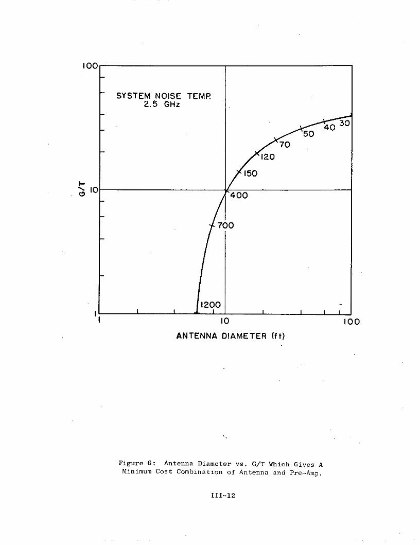
100

SYSTEM NOISE TEMP2.5 GHz

4030S4"50

70

1212000

150

10

400

700

1200I I I I I I

10 100

ANTENNA DIAMETER (ft)

Figure 6: Antenna Diameter vs. G/T Which Gives AMinimum Cost Combination of Antenna and Pre-Amp.

III-12

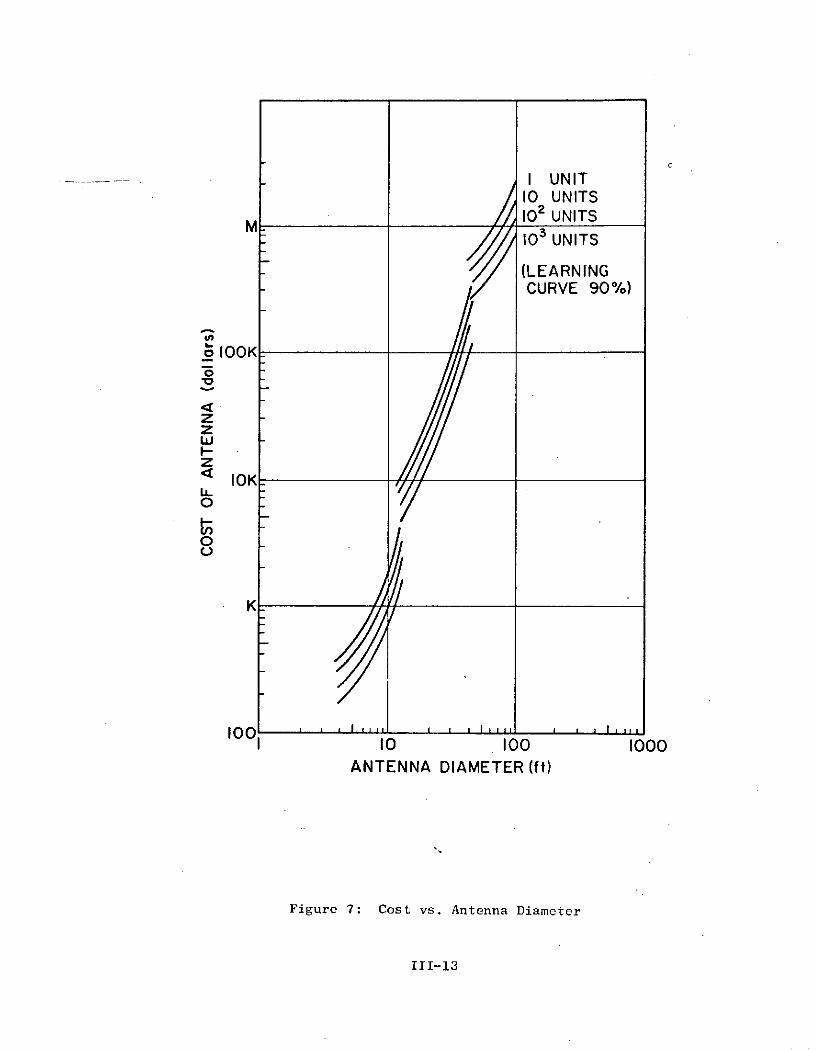
I UNIT10 UNITS

M I10 UNITS

10 UNITS

(LEARNINGCURVE 90%)

o lOOK

zzwF-z4 IOK

0

10 0 1 1 1 , , f iS10 100 1000

ANTENNA DIAMETER (ft)

Figure 7: Cost vs. Antenna Diameter

III-13

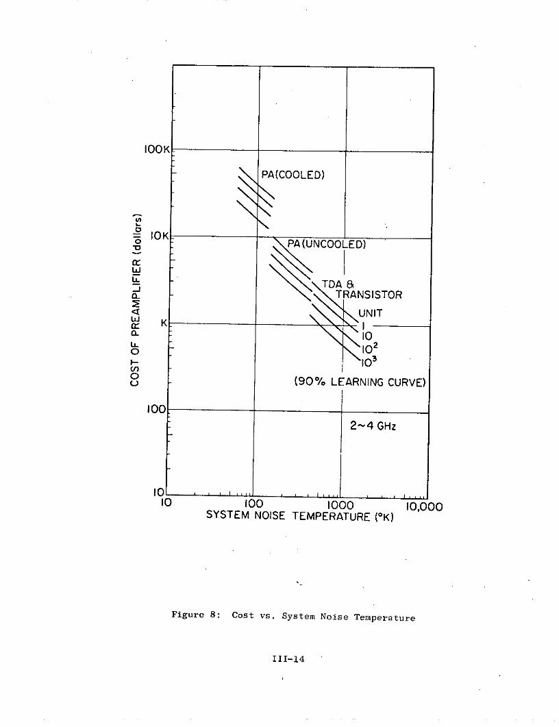
lOOK

PA(COOLED)

IOK10o PA(UNCOOLED)

TDA &-J-

a TRANSISTOR

UNITr K I

U- _1020- 1

,10

- (90% LEARNING CURVE)

100

2-4 GHz

10 100 1000 10,000SYSTEM NOISE TEMPERATURE (OK)

Figure 8: Cost vs. System Noise Temperature

III-14

106

0

IO

<10

WI-

z

10 I 2.5 GHzo 000 UNITL)

10

0 10 20 30 40 50G/T (dB/OK)

Figure 9: Cost of Antenna and Pre-Amplifier vs. G/T

III-15

the number of receiving stations and the relative importance attached

to the complexity and cost of the space segment vs. the earth segment.

Thus, the satellite communication system cost can be minimized by

trade-offs between ground station antenna size and satellite EIRP for

a given frequency.

It seems that the future trend will be toward the use of higher

EIRP satellites with larger numbers of ground stations having correspon-

dingly reduced cost.

The per-channel EIRP required for a link is given by:

EIRP = C/T + Lp + L m + M - (G/T)e

where

EIRP : Satellite effective isotropic radiated power

C/T : Carrier-power to system noise temperature ratio

Lp : Path loss in the link

Lm : Miscellaneous losses in the link

M : Desired operating margin

(G/T)e : Antenna gain to system noise temperature ratio atthe earth-station receiver input

Fig. 10 shows a curve of EIRP vs. G/T with C/T as a parameter for

a ground-station antenna elevation of 10 degrees at 2.5 GHz. It was

assumed that L. = 1.5 dB, and M = 2.5 dB. The ratio C/T is determined

by the nature and quality of the desired signal. Values of interest

range from C/T = -190 dBW/oK for a low bit rate data channel to C/T =

-140 dBW/oK for a high quality TV channel. This relation is important,

essentially determining the satellite and earth terminal configuration.

J. Cost vs. Transmitter Power

The cost of power amplifiers changes depending upon the output power

and bandwidth, the type of amplifier, the number of carriers to be trans-

mitted, etc. Generally speaking, the cost increases with increasing

output power. The power amplifier alternatives are listed in Table 3.

111-16

80

70

60

50

-O40 \ \

2.5 GHz

-190 -180 -170 -160 -150 -140 -30

0 10 20 30 40 50 60 70 80G/T (dB/°K)

Figure 10: EIRP vs. G/T for given C/T

III-17

Table 3: Power Amplifier Alternatives

Power Amp. Type Output Power Bandwidth

Klystron High Narrow

Traveling Wave Tube Medium Wide

Transistor Low Wide

Fig. 11 is a plot of power amplifier cost encountered in the survey

as a function of their out power. A smooth curve of cost vs. output

power is presented in Fig. 12.

K. Installation Cost

The installation costs consists of shipping charges and labor costs

for equipment installation, a power plant, water supply facilities,

grading road construction.

Installation, material, and labor range from 15 to 30 percent of

the equipment cost depending on the size and importance of the station,

the provision of standby equipment, and the availability of any existing

power supply. Considering stations of small channel capacity, the maxi-

mum station demand will be 10 to 50 KVA, while medium and large traffic

capacity station will demand in the range of 200 to 500 KVA. Main power

is typically purchased from a commercial supplier with standby power

provided by one or more diesel-generator sets.

Commercial power lines may cost from $10,000 to $20,000. Standby

power supplies will range from 8 to 15 percent of total hardware cost.

When the system is installed in relatively inaccessible or remote

locations, the installation cost, of course, increases. It is assumed

that the installation cost, including only material and labor, is 15

percent of equipment cost for small antennas, 20 percent for medium

size antennas, 30 percent for large antennas, and 15 percent for other

equipment. Power provision, water supply facilities and their installa-

tion and road construction costs are assumed to be 15 percent of the

initial capital investment.

The cost of power provision, water supply and road construction is

shown in Fig. 13. Fig. 14 shows the cost vs. G/T including installation.

III-18

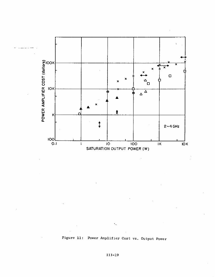
C

IOOK x x

0 x- x

0 xU 0- IOK x

,--w d

I I Aa.

SxA

cc

3: K0n K

2-4 GHz

100

0.1 10 100 IK IOKSATURATION OUTPUT POWER (W)

Figure 11: Power Amplifier Cost vs. Output Power

III-19

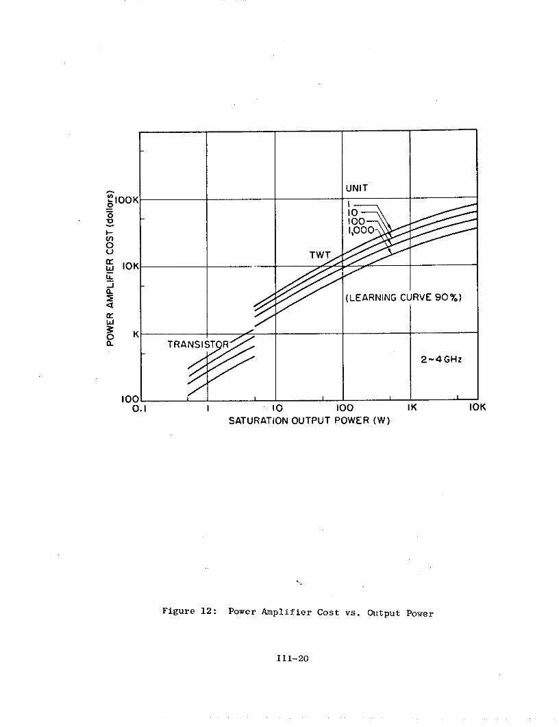
UNITIOOK

-OK(J

2 I (LEARNING CURVE 90%)

0 K

. K TRANSIST R

2-4GHz

100 1 I I0.1 I 10 100 IK IOK

SATURATION OUTPUT POWER (W)

Figure 12: Power Amplifier Cost vs. Output Power

III-20

-,

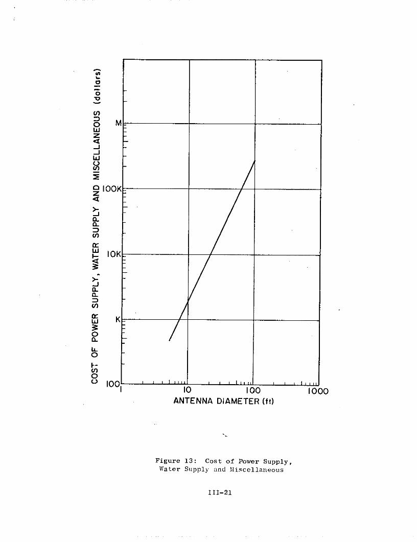
O

0 OOKz

w

IOK

-L -

a-a

D

c)

O IOK

-J-

aa.c,

W K

oa

0

0O 10 0 1 , , , , , , Ii ,

10 100 1000ANTENNA DIAMETER (ft)

Figure 13: Cost of Power Supply,Water Supply and Miscellaneous

III-21

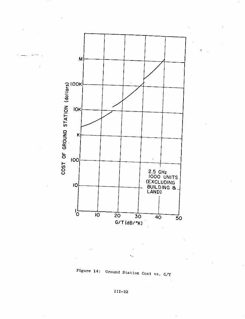
M

SIOOK

o

O .z K0

O

0

100

oIC 2.5 GHz1000 UNITS

(EXCLUDINGIO BUILDING 8

LAND)

0 10 20 30 40 50G/T (dB/OK)

Figure 14: Ground Station Cost vs. G/T

III-22

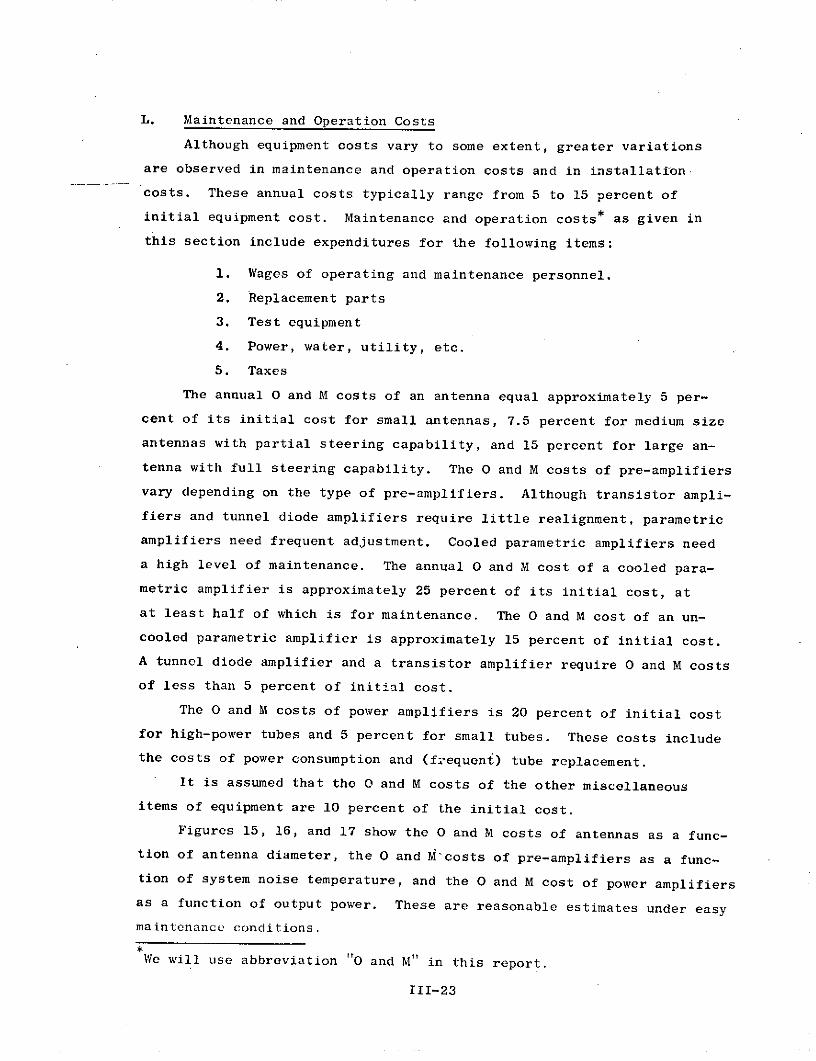
L. Maintenance and Operation Costs

Although equipment costs vary to some extent, greater variations

are observed in maintenance and operation costs and in installation-

costs. These annual costs typically range from 5 to 15 percent of

initial equipment cost. Maintenance and operation costs* as given in

this section include expenditures for the following items:

1. Wages of operating and maintenance personnel.

2. Replacement parts

3. Test equipment

4. Power, water, utility, etc.

5. Taxes

The annual 0 and M costs of an antenna equal approximately 5 per-

cent of its initial cost for small antennas, 7.5 percent for medium size

antennas with partial steering capability, and 15 percent for large an-

tenna with full steering capability. The O and M costs of pre-amplifiers

vary depending on the type of pre-amplifiers. Although transistor ampli-

fiers and tunnel diode amplifiers require little realignment, parametric

amplifiers need frequent adjustment. Cooled parametric amplifiers need

a high level of maintenance. The annual 0 and M cost of a cooled para-

metric amplifier is approximately 25 percent of its initial cost, at

at least half of which is for maintenance. The O and M cost of an un-

cooled parametric amplifier is approximately 15 percent of initial cost.

A tunnel diode amplifier and a transistor amplifier require 0 and M costs

of less than 5 percent of initial cost.

The O and M costs of power amplifiers is 20 percent of initial cost

for high-power tubes and 5 percent for small tubes. These costs include

the costs of power consumption and (frequent) tube replacement.

It is assumed that the 0 and M costs of the other miscellaneous

items of equipment are 10 percent of the initial cost.

Figures 15, 16, and 17 show the O and M costs of antennas as a func-

tion of antenna diameter, the 0 and M'costs of pre-amplifiers as a func-

tion of system noise temperature, and the O and M cost of power amplifiers

as a function of output power. These are reasonable estimates under easy

maintenance conditions.

We will use abbreviation "0 and M" in this report.

III-23

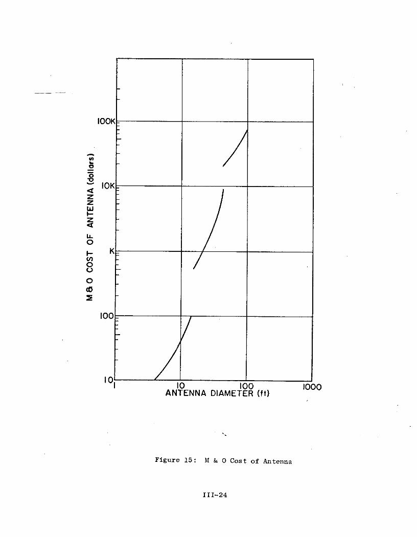
IOOK

zzOZ-

0-- K

I00

101 10 100 1000

ANTENNA DIAMETER (fl)

Figure 15: M & 0 Cost of Antenna

III-24

IOK

0

SIOK

.j _

wa

0 KI-

o

u

100

10 I II0 100 1000 10,000

SYSTEM NOISE TEMPERATURE (OK)

Figure 16: 0 & M Cost of Pre-Amplifier

III-25

o

IOOK

0

- IOK

W

0

U.

-J

0 K

o -I0

o T RANSISTOR

100.1 0 100 IK IOK

SATURATION OUTPUT POWER (W)

Figure 17: 0 & M Cost of Power Amplifier

111-26

M. Site and Building Costs

The site and building costs depend on the location and increase

with increasing antenna diameter. A typical cost of buildings for tele-

communications stations is approximately $20 per square foot. The cost

of land ranges from $5,000 to $50,000 depending on the location.

It is estimated that a small station needs 100 to 500 square feet

of building and 0.02 to 0.05 acres of land. Also, it is estimated that

a large station needs 10,000 to 20,000 square feet of building and 2 to

5 acrea of land. Fig. 18 shows the cost of the building as a function

of antenna diameter. Fig. 19 shows the site cost as a function of an-

tenna diameter.

III-27

M

OOK K.o

0

IO

K

S10 100 1000ANTENNA DIAMETER (ft)

Figure 18: Building Cost of Ground Station

III-28

M

IOOK7,

OU

zCm IOK-J

10010 100 1000

ANTENNA DIAMETER (ft)

Figure 19: Site Cost of Ground Station

III-29

N. Conclusion

We have developed the satellite communication ground station costs

from a survey of existing ground stations, sales catalogs, and literature.

Using this basic cost information, smooth curves of cost vs. antenna

diameter, cost vs. system noise temperature, and cost vs. transmitter

output power were derived. The figures presented make no attempt to

predict cost reductions that may occur in the future as a result of im-

proved technology or novel mass-produced designs. Rather, they reflect

the cost of presently available commercial equipment.

III-30

O. REFERENCES

1. Milne, K. and J.L. Blonstein, "The Economics and Applications of

Small Earth Stations," U.K. Seminar of Communication Satellite

Earth Stations--London, May 1968.

2. Pope, D.L., "Parametric Representation of Ground Antennas for

Communication Systems Study," BSTJ, Dec. 1968.

3. Janky, J.M., "Optimization in the Design of a Mass-Producible

Microwave Receiver Suitable for Direct Reception from Satellite,

Stanford Electronics Laboratories, Tech. Report No. 3683-1.

4. ASCEND, Stanford University, 1967.

5. Pope, D.G., "Economic Aspect of Data Transmission by Satellite,"IEEE Convention, 1969.

6. Emerson, J., "Factors Affecting the Choice of High Power Amplifiers

for Satellite Earth Stations," IEEE Conference Publication No. 72.

7. Cosgrove, T., "Economic Considerations for Communication Systems,"

IEEE Trans. COM-16, No. 4, Aug. 1968.

8. Talyzin, N.V. et. al., "Optimum Power Parameters and Economic

Efficiency of a Comnunication-Satellite System," Telecommunication

Journal, Vol. 38, V/1971.

9. Aitchison, C.S., "Parametric Amplifiers Designed for ReceivingSystems," Electronic Engineering, June 1971.

10. Kakihana, S., "Transistors for the Era of Microwave Communication,"WESCON '71, 26/3.

11. Building Costs, Vol. 21, No. 6.

12. Standard Industrial Survey Report, Jan. 1970.

III-31

CHAPTER IV

SATELLITE SEGMENT COSTS

A. Introduction

Since the teleconferencing systems we are considering have a large

number of remote ground stations, minimizing the total space-segment

cost implies that these stations be inexpensive - hence of low sensitivi-

ty. Under these conditions, the system is "power-limited" so that, for

a given area of coverage, total satellite RF power* is the scarce resource

of the space segment. We wish to estimate the lowest reasonable cost

of this resource: i.e., the annual cost per RF Watt.

One approach to this problem is to fit a curve to historical data.

Between the data points, a cost model can be employed to generate a con-

tinuous function of cost/watt vs. total watts. Such models are based on

the fact that the cost of a satellite in orbit is primarily determined by

its weight, which in turn is highly correlated with its total RF power.1

But such a trend approach is not realistic for our application since

we are interested only in contemporary (or near-future) system components.

Instead, we shall examine a contemporary "shopping list" of satellites;

and the launch stream of each needed to satisfy a given demand growth.

We posit three types of demand functions (constant, linear, and a com-

bination of both); and two spare-backup strategies (orbit spare and

ground spare). For each case, we then calculate the present value of the

required investment stream as a function of the discount rate. Finally,

we compute the annual cost (or price) which must be charged to recover

the invested capital. We will choose that launch stream which has the

lowest annual cost per RF Watt..

We assume that this total power can be partitioned into as many trans-ponders as desired--bounded, of course, by FCC and CCIR bandwidth re-straints. We determine the power per teleconferencing transponder byminimizing total system cost for a given number of teleconferencingtransponders (say, 4). If the resulting total teleconferencing RFpower is less than the total satellite power, we assume that the sur-plus will be channeled into additional transponders and sold to othermarkets (i.e., non-dedicated use).

IV-1

B. Methodology

Many of the satellites now in orbit or proposed for near-future launch

are possible candidates for teleconferencing use - either as configured now,

or as reconfigured appropriately vis-a-vis beam coverage and frequencies.

Table 1W is a representative listing of these candidates. Also given (see

last column) is the per-watt investment, assuming one in-orbit satellite,

for each case.

These data alone might suffice for a rudimentary analysis. But a more

accurate assessment of space segment costs must include the effects of

(1) Supply and demand time-profiles

(2) Economies of scale

(3) The time value of money

(4) Gracefulness of system degradation

(5) Reliability (failure rate)

(6) Flexibility to changing demands and technology.

The analysis which follows treats (1), (2), (3), explicitly; and develops

a general methodology for treating the effects of(4), (5), and (6). Three

demand models are developed. Then the launch-stream investment necessary

to meet these demands is calculated on a present-value basis. This is done

for several discount rates and for two system "back-up" strategies. Finally,

annual cost-per-watt is computed as the zero profit price an entity (presumably,

the satellite owner) would charge to recover its invested capital for a given

demand growth.

1.Three Candidate Satellites: Small, Medium and Large

To keep the analysis within bounds, our shopping list must be culled. We

desire comtemporary satellite designs either already suited for teleconferencing

use, or easily modified. Moreover, we would like to examine cases which span

wData sources include References 2, 3, 4, 5, and 6.

IV-2

TABIB 1: SATELLITE ATTRIBUTES AND COSTS

Total Ie~estretIm

Investment Cost ($ a I e -orbstlTotal Fre-

4 Satel*

o Iamber Tres-? Total prim Desg seoates- for one i -orbit

Weight (th.) la h quency lite of ponder g6nd- Power Life porary launch Costs Satellite Coste Dovel- I t (atellite -orbit pa Vehicle Power nds supples Tran- indwdth width (D.C. (years) i b irst ube opnt Co Total att

n:lders (AIl) (Sl.) watt) nt Coustt CotsTotal Watt

IWTISAT I 5 150 Thrust- - C Rugho 2 (15) 30 1.8 3.3 3.3 7.4 3. n.. - 10.7

II 160 3 r7 Augoentd 18 C Sulh.. 1 130 130 - 3 3. 3. 4.1 3.5 a.0. 7.6 .422

Ill 280 647 Delts 20 C W 2 225 450 - 6 .1 5.1 4.0 4.6 a.e. 9.1 .455

5S-333: TEI.SAT 10 1206 1 Thor Delta 60L

8 8 Includod - 15.0 .300

TELSAT - Alaska 10 1206 MGT 010 Ic RuIhee 121 136 1 4321 12201 11 1 10 2 - 17.0 .340anghts D) 453 1120 Thor I.ite MCr 60 v Iludd 13.0 .21easter, Unio ( )] 510 - 1hur Delt M 00 il 11 13 13.0 .216

RS-336 598 1560 Thor 0Dl tUpgroad 88 8 Hughes - 190 - -10 0 7 7 6.3 (6.3) (9.4) (.0) 21.7 .247

RCA [D1 638 1412 hor L l.ts 904 60 C RCA 1 36 432 403 7 . 1.3 7.3 3.6 3.6 14.8 1.3 25.7 .429

WrCI (D) 663 1446 Thor I Its 2914 60 C.K N.A.R. 13 36 432 T 7 7.5 7.9 8 15I .5 26.5 .475ATS - 775 - :.s 1 C I Huhe 2 23 0 - a..I

39 - As D 25 50 -

ITEELSAT IV 1225 3058 Atlas Centaur 120 C Hughes 12 36 4323 - 16. 16 10 (9) - 37.0 .309

COMSAT [D) 1650 3100 Atlas Centaur 89 C - 24 38 816 .40 7.16 . 17.9 13.8 13. 13 .9 2.7 45.3 .509

ATS - F .1900 2600 Titan IIIC 16 S.C. - - - 2.5 ..

SG* -.200 -lH . 50" 0 25.7 25.7 14.7 14.7 16.6

Fairchild-Bill.r (D .2600 2903 TlIta MC Uprete 95 8.C.K T-5 10 36 750 V V 25.1 25.1 14.7 14.7 16.6 8.3 57.0 .6

CI - Lochhed (DJ 3900 - Tine DID Ages 67 C Lackhead 4 36 1758 4400 to v 22.8 21.7 20.6 20.6 30.2 1.5 73.6 .109

4 - . VIIF; m 2.5 s; C A 4/6 GUass K. 12/13 GOs; 9 - For two or me actIe satelliteaI rNTY a.a. - sot applicable A mlllester 10 - Assumed to be the se as Western Untom- - unknown 8 - 7/13 Gt1 used instead of 12/13 06( 11 - Western Union will pay Hughes $47.72 a

(D) - Doestle filing.s -* - Ito Fairchild Iller; N.A.R. to North American Rockwell for 5 satellites and 3 launche.; or* * 3-axis stabilizd 7 - Useable (- -1 d4) Bandwidth about $26.7 a for 5 ughs satellites,1 - 8pn-otbilevd option (similar to 118-333) - Illude range support lncluding developmeat and TTrc costs.I - Approit.e: =,.O weights apply aftor apogee l - Include. doelopoent costs; secludes

actor tire and ere higher than fin1al -orbit ( ) - pproximate (dedweed) IAC ost.

3 * lad-of-Ht e total RF power

IV-3

extremes in total RF power. With these criteria in mind, the field can

be narrowed to three.:

RF D. C.

In-Orbit Launch No. of 36 MHz Total PrimeSize Satellite Weight (ibs) Vehicle Transponders Power Power Efficien,

Small HS-336 598 Thor Delta .12 88W 220W .4(Upgrade)

Medium Intelsat IV 1225 Atlas Centaur 12 120W 740W .16

Large MCI-Lockheed 3900 Titan IIID 48 672w 4.4kW .15Domestic Filing Agena

The satellites are quite similar in basic design although the MCI-Lockheed

satellite differs by being three-axis stabilized and by operating half of its

transponders at 12/13 GHIz (the other two are spin stabilized and operate at 4/6

GHz or 2.5/6 GHz). Note that the Hughes design has a higher efficiency (ratio of

RF power to prime power). For our purposes, these differences are relatively

minor.

Approximate cost data are re-summarized as follows:m

First Launch First Satellites DevelopmentLaunch Thereafter Satellite Thereafter Costs

Satellite ($M) ($M) ($M) ($M) ($M)

Hughes HS-336 7 7 6.3 6.3 8.4

Intelsat IV 16 16 12 10 9

MCI-Lockheed 22.8 21.7 20.6 20.6 30.2

These data were obtained either from published figures (See References)or from knowledgeable sources. Those from the latter are credible estimatesbut cannot be considered hard quotes.

IV-4

These cost data are estimates; and they will vary with time as well as

with application. Our conclusions, therefore, although based on specifics,

must be considered generic; and they are valid only for the data used.

However, the methodology developed below can be applied in general.

2. Supply and Demand Functions

Consider three general types of demand growth over time: (1) constant

demand, (2) linear growth over a specified span; constant demand thereafter,

(3) linear demand growth forever. These three demand functions and the various

launch streams necessary to satisfy them are summarized in Fig. 1. A ten-year

lifetime is assumed for all three satellites.

These supply and demand functions allow us to examine tradeoffs between

scale economies and the time-value of money. Indeed, most of

the demand curves have been shaped to facilitate an economic comparison of small,

medium, and large satellites. We are assuming implicitly here that capacity is

proportional to total RF power (power-limited operation). For teleconferencing

applications (small ground stations))this is not an unwarranted assumption.

Note that the large satellite has about six times the capacity of the medium

one, and about eight times the capacity of the small one. (This comparison would

be exact if MCI were 700 Watts; Intelsat IV, 116.7 Watts; and Hughes, 87.5 Watts.)

3. Economies of Scale

We can examine economies of scale explicitly by expressing the costs of

the larger satellite in terms of the costs of the smaller:

Intelsat IV is quoted at 7 years, but we feel that a "medium" satellite ofits characteristics will have at least a ten-year lifetime by 1975.

IV-5

TOTALWATTS (a)- (b)704672

L : 8 small satellites, launchedDI together, every 10 years,

foreverLb: 1 large satellite launched

every 10 years, foreverL : 1 small satellite, launched88 c

SI every t l0 years, forever

S2 4 6 8 I0 ...... years

TOTAL )WATTS (d) (b)720L L Ld: 1 small satellite, launched704- d every 1 1/4 years, forever

/2 L: 1 large satellite, launchedevery 10 years, forever

D2 L : 1 medium satellite, launchedevery 1.67 years, forever

0 2 4 6 8 I0.- years

) , L : 1 small satellite launched every 1 1/4years 0 <t< 10

72--4 - 2 small satellites launched every 1 1/4years 10 t< 203 small satellites launched every 1 1/4

D3 years 20< t< 30 etc.

Lf: 1 large satellite launched at t=Of 2 large satellites launched at t=103 large satellites launched at t=20 etc.

0 2 4 6 8 I0----- . years

Figure 1: Supply and Demand Functions

IV-6

Larger Smaller

Development Costs: sD x D

Satellite Costs: S F x Sss s

Booster Costs: BsFBx Bs

where x is the number of smaller satellites needed to produce the same

total RF power (i.e. capacity) - as the larger; and where the efficiencies

F account for the fact that increasing satellite capacity by, say 8 times,does not (usually) increase its cost by as much as 8 times. If the F's are

_1, there are diseconomies of scale.

Using the data presented earlier above for the three satellite cases,

we can deduce the economies of scale for each pairwise combination:

x=8 x-6 x=l.365Larger = IMCI Larger=MCI Larger=Int.IVSmaller=HS-336 Smaller=Int.IV Smaller- HS-336

Development FD 5 .56 .782

Satellite Fs .41 .286 1.4

Booster Fg .407 .238 1.68

We concluded that the large satellite enjoys considerable economies of

scale over both the small and the medium satellite. The medium satellite has

diseconomies for the data given mainly because its total power is low for the

launch vehicle used. The time-value of money may alleviate these diseconomies,

but will benefit the small satellite still more. We expect, therefore, that

the medium satellite will be an uneconomical choice on the basis of cost per

RF Watt. Because of this, we have relegated the economic analysis of the

,t1,lMit lin ;: Il.llI i i, l Cl.', (lllltil h till '1 )1 ill I'.. i) ,I Ap',,eell .1. ii. 'l'l, 1.).J 1

of this appendix corroborate our tentative conclusion.

IV-7

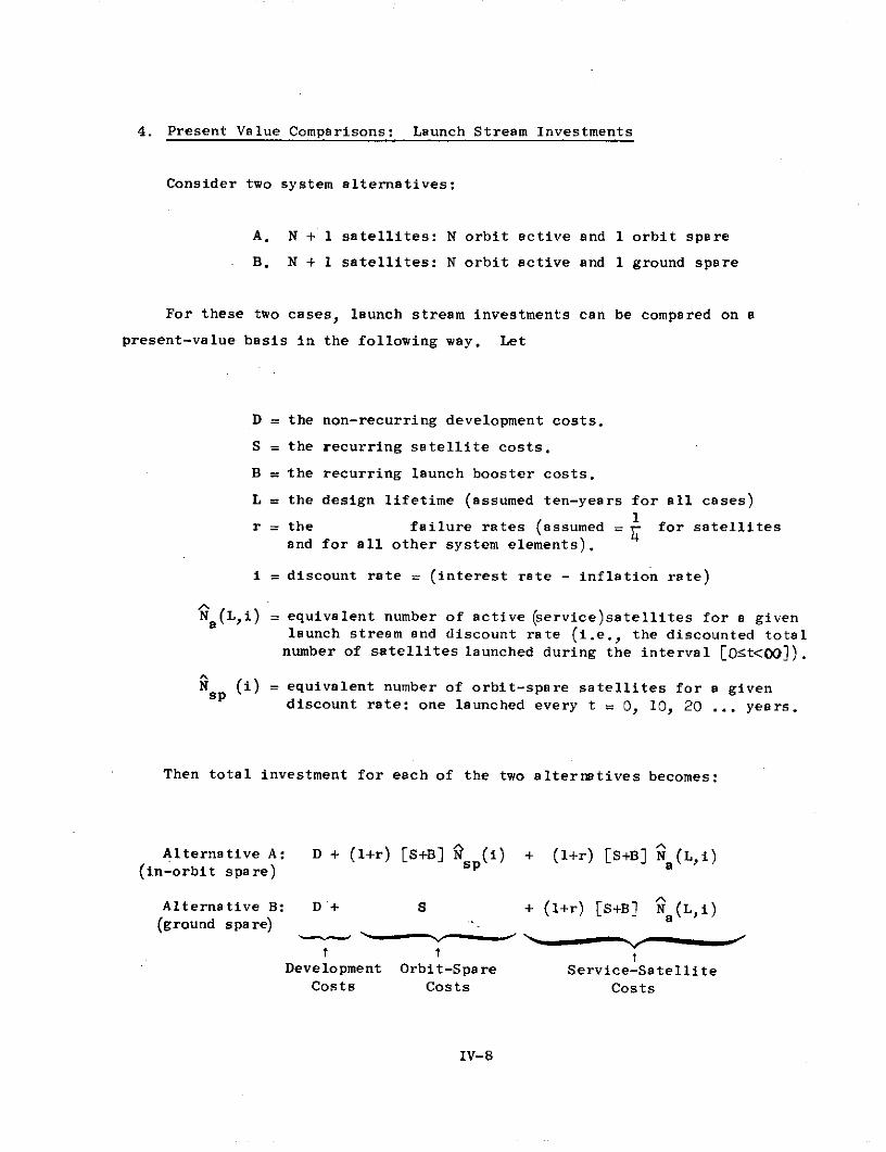
4. Present Value Comparisons: Launch Stream Investments

Consider two system alternatives:

A. N + 1 satellites: N orbit active and 1 orbit spare

B. N + 1 satellites: N orbit active and 1 ground spare

For these two cases, launch stream investments can be compared on a

present-value basis in the following way. Let

D = the non-recurring development costs.

S = the recurring satellite costs.

B = the recurring launch booster costs.

L = the design lifetime (assumed ten-years for all cases)

r = the failure rates (assumed = for satellitesand for all other system elements).

i = discount rate = (interest rate - inflation rate)

Na (L,i) = equivalent number of active (service)satellites for a givenlaunch stream and discount rate (i.e., the discounted totalnumber of satellites launched during the interval [0 t<00]).

N (i) = equivalent number of orbit-spare satellites for a givendiscount rate: one launched every t =0, 10, 20 ... years.

Then total investment for each of the two alternatives becomes:

Alternative A: D + (l+r) [S+B] !R(i) + (1+r) [S+B] N (L,i)(in-orbit spare) a

Alternative B: D+ S + (l+r) [S+B] N (L,i)(ground spare) a

a tDevelopment Orbit-Spare Service-Satellite

Costs Costs Costs

IV-8

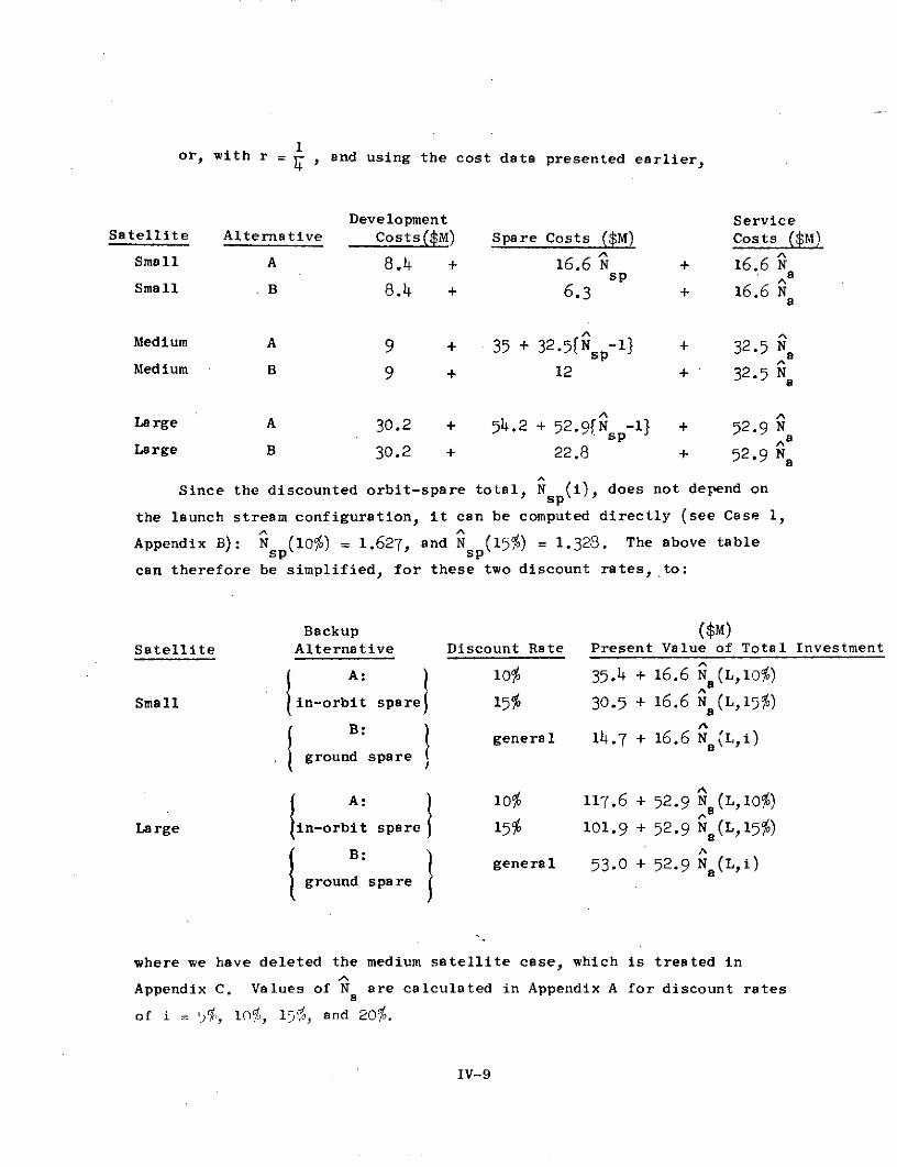
or, with r = , and using the cost data presented earlier,

Development ServiceSatellite Alternative Costs($M) Spare Costs ($M) Costs ($M)

Small A 8.4 + 16.6 N + 16.6 Nsp ^a

Small B 8.4 + 6.3 + 16.6 Na

Medium A 9 + 35 + 32.5[N p-1 + 32.5 Nsp ~aMedium B 9 + 12 + 32.5 Naa

Large A 30.2 + 54.2 + 52.9fN -1 + 52.9 N

Large B 30.2 + 22.8 + 52.9 Na

Since the discounted orbit-spare total, Nsp(i), does not depend on

the launch stream configuration, it can be computed directly (see Case 1,AA

Appendix B): N sp(10) = 1.627, and N p(15%) = 1.328. The above table

can therefore be simplified, for these two discount rates, to:

Backup ($M)Satellite Alternative Discount Rate Present Value of Total Investment

A: 10% 35.4 + 16.6 Na(L,10%)

Small in-orbit sparej 15% 30.5 + 16.6 Na(L,15%)

B: general 14.7 + 16.6 N aL,i)ground spare I a

A: ) 10% 1176 + 52.9 Na(L10%)

Large in-orbit spare 15% 101.9 + 52.9 N (L,15%)

B:ground spare general 53.0 + 52.9 N a(L,i)

ground spare

where we have deleted the medium satellite case, which is treated in

Appendix C. Values of N are calculated in Appendix A for discount ratesa

of i = L%, 10%, 15%, and 20%.

IV-9

5. Annual Cost: Zero-profit pricing

We derive annual cost (or price) per watt for a given discount rate

and investment stream by calculating the annual lease payments to the

satellite-owner necessary to ensure recovery of his capital. We assume that

the"owner" (who may be fictitious) will be satisfied with a zero profit.

Then the present value of the lease payment stream must equal the present

value of the capital outlay:

A

PV(revenues) = C . W(D,i) = PV(investment)

where C = annual cost (or lease price) per watt (dollars per watt per yea

AW (D,i) = effective (discounted) total RF power sold.

The amount of sold power (or capacity) at a given time depends entirely

upon assumed demands; while the discounted total sold capacity depends not

only upon the demand function, but the interest rate as well. (We must discount

the total sold capacity because payments far in the future are less valuable to

the "owner" then payments he receives now). Values of the discounted total,

W (D,i) are computed in Appendix B for i = 5%, 10%, 15% and 20% and for all

prescribed demand functions.

Note.that annual operating and maintenance costs have been ignored: they

are not crucial and will, in any event, be relatively invariant to changes in

the launch stream strategies.

C. Results and Conclusions

Table 2 summarizes the results from Appendices A and B for discount rates

of 10% and 15%. As expected for non-zero interest rates, the discounted supply

and demand totals are finite even though the supply and demand streams are

infinite.

IV-10

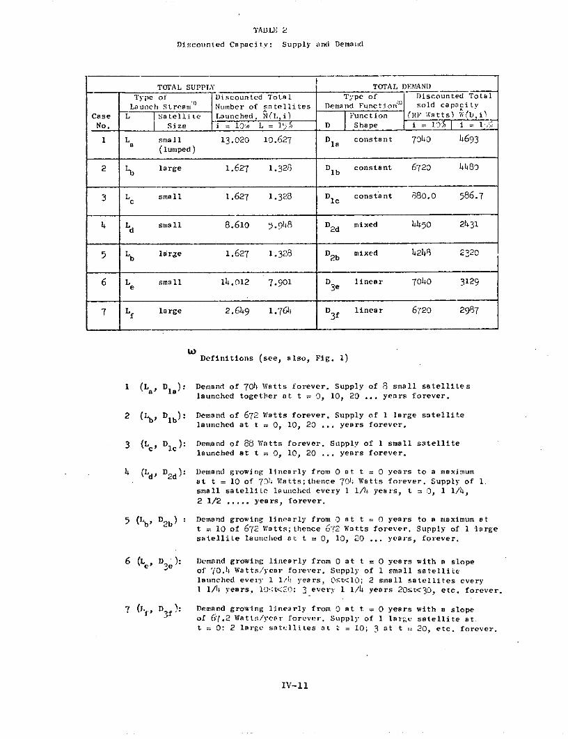
TABU 2

Discounted Capacity: Supply and Demaind

TOTAL SUPPLY TOTAL DE.MAND

Type of Discounted Total Type of Discounted Total

Launch Streamw' l Number of satellites Demand Function'j sold capacityCase L Satellite Launched, N(Li) Function (RF Watts) W(D,i%

No. Size 10' L = 1 D Shape i = 1.. 71 i = 1

1 L small 13.020 10.627 D constant 7040 4693(lumped)

2 large 1.627 1.328 Dlb constant 6720 4480

3 Lc small 1.627 1.328 Dlc constant 880.0 586.7

4 Ld small 8.610 5.948 D2d mixed 4450 2431

5 Lb large 1.627 1.328 D2b mixed 4248 2320

6 Le small 14.012 7.901 D3e linear 7040 3129

7 Lf large 2.649 1.764 D3f linear 6720 2987

Definitions (see, also, Fig. 1)

1 (La, Dla): Demand of 70)4 Watts forever. Supply of 8 small satellites

launched together at t = 0, 10, 20 ... years forever.

2 (Lb, Dlb): Demand of 672 Watts forever. Supply of 1 large satellitelaunched at t = 0, 10, 20 ... years forever.

3 (Lc, D1 c): Demand of 88 Watts forever. Supply of 1 small s3tellitelaunched at t = 0, 10, 20 ... years forever.

41 (ld, D2d): Demand growing linearly from 0 at t = 0 years to a maximum

at t = 10 of 704 atts;thence 704 Watts forever. Supply of 1.small satellite launched every 1 1/4 years, t = 0, 1 1/4,2 1/2 ..... years, forever.

5 (Lb, D2b) : Demand growing linearly from 0 at t = 0 years to a maximum att = 10 of 672 Watts;thence 672 Watts forever. Supply of 1 iargesatellite launched at t = 0, 10, 20 ... years, forever.

6 (Le, D.e): Demand growing linearly from 0 at t = 0 years with a slopeof '10. Watts/year forever. Supply of 1 small satellitelaunched every 1 1. )4 years, O0t<10; 2 small satellites every1 1/4 years, 10:t<20; 3 every 1 1/4 years 20!t<30, etc. forever.

7 (i.f, D f): Demand growing linearly from 0 at t = 0 years with a slopeof 6'1.2 Watts/yepr forever. Supply of 1 large satellite at.t = 0: 2 large satcllites at t = 10; 3 at t = 20, etc. forever.

IV-11

Table 3 summarizes present values of investments and annual costs per

watt for all prescribed launch strategies, supply and demand functions, and

for discount rates of 10% and 15%.

Figures 2, 3, and 4 depict these results graphically and extend them for

discount rates of 5% and 20%.

IV-12

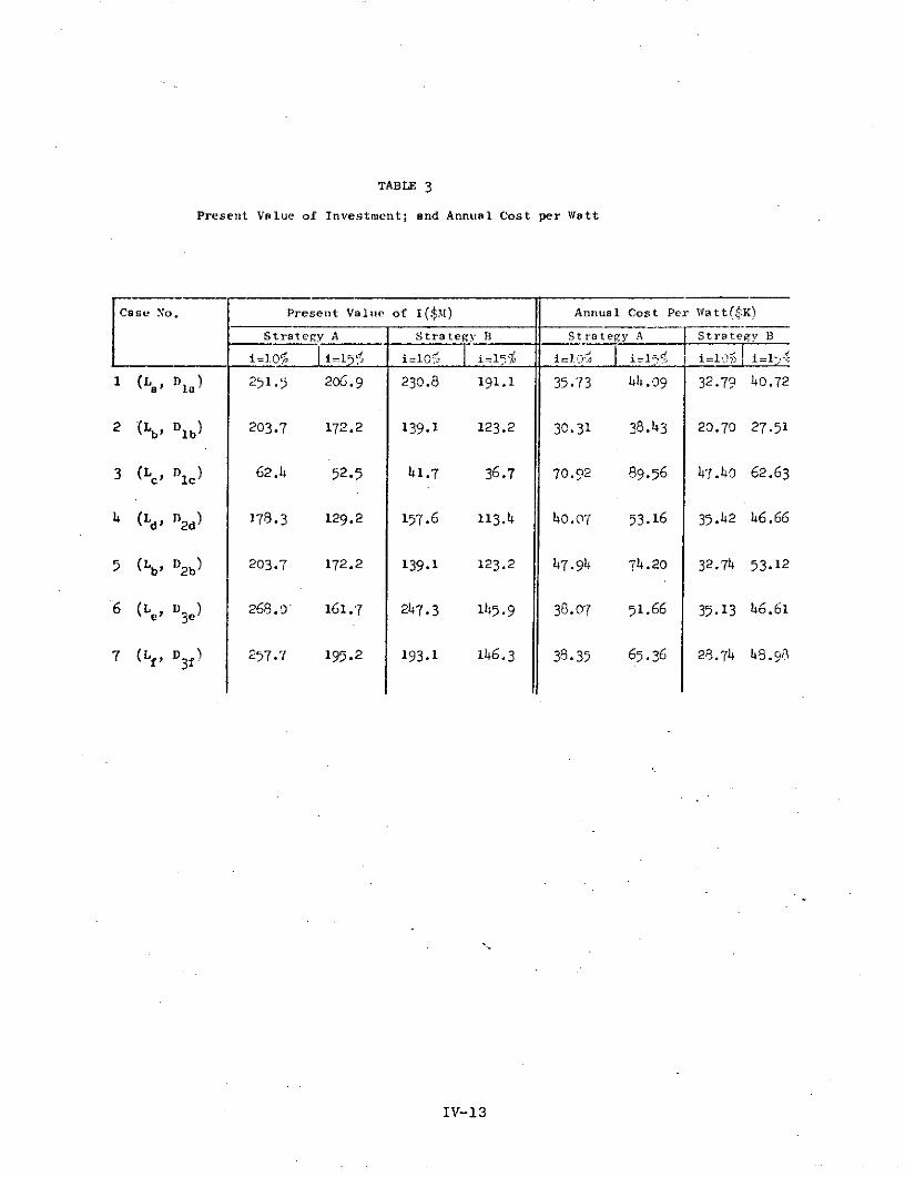
TABLE 3

Present Value of Investment; and Annual Cost per Watt

Case No. Present Value of I($MI) Annual Cost Per Watt($K)

Strategy A Strategy B Strategy A Strategy B

i=1.0 i=1Ydi i=10 i=15 i=1.o i 1 - i=1o iI=I

1 (L, D1a) 251.5 206.9 230.8 191.1 35.73 44..39 32.79 40.72

2 (Lb, Dib) 203.7 172.2 139.1 123.2 30.31 38.43 20.70 27.51

3 (Lc, Dlc) 62.4 52.5 41.7 36.7 70.92 89.56 47.40 62.63

4 (Ld, D2 d) 178.3 129.2 157.6 113.4 40.07 53.16 35.42 46.66

5 (L , D2b) 203.7 172.2 139.1 123.2 47.94 74.20 32.74 53.12

6 (Le, D3e) 268.0 161.7 247.3 1145.9 38.07 51.66 35.13 46.61

7 (Lf, D 3f) 257.7 195.2 193.1 146.3 38.35 65.36 28.74 48.9A

IV-13

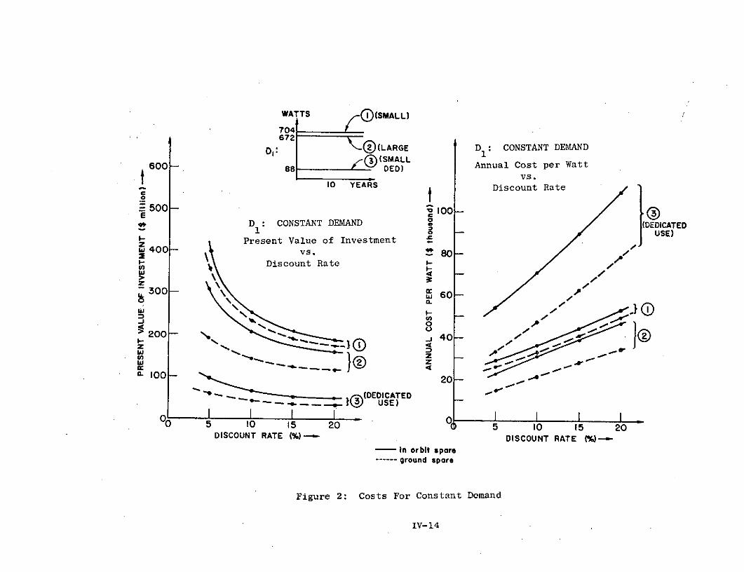
WATTS (SMALL)

704672

D: 3 (LARGE D1 : CONSTANT DEMAND

600 DED) Annual Cost per Watt1 0 YEARS vs.

10 YEARS Discount Rate

500 - ^ 100 -D CONSTANT DEMAND (DEDICATED1 -USE)

z Present Value of Investment fS400 - vs

Discount Rate

300 -0 -w 60

200 - 40

20 -

--00- -( DEDICATED 20

S 5 10 15 20 5 10 15 20DISCOUNT RATE (%)- DISCOUNT RATE (%)---

- in orbit spare------ ground spare

Figure 2: Costs For Constant Demand

IV-14

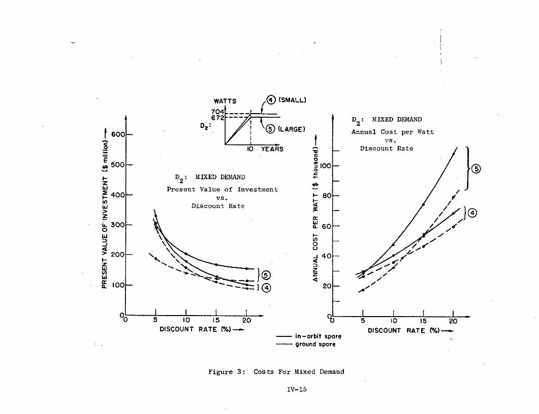
WATTS ® (SMALL)

704___672--- D2 : MIXED DEMAND

600 D2: (LARGE) Annual Cost per Watt0

vs.-o 10 YEARS L Discount Rate

E 500 - 100 -D : MIXED DEMAND

z2 40)bl Present Value of Investment2 400- vs 80-

w Discount Rate

iL. 300- 60- /

z D

w z ,

SO - -. ) 20

0o 5 10 15 20 5 10 15 20DISCOUNT RATE (%)-- DISCOUNT RATE (%)-.-

- in-orbit spare------ ground spore

Figure 3: Costs For Mixed Demand

IV-15

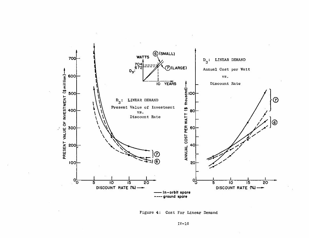
WATTS700 WATTS D3: LINEAR DEMAND704 ----

D672 7 (LARGE) Annual Cost per Watt

600 vs.

10 YEARS Discount Rate

500 - 8 100 -z5 0 D3 : LINEAR DEMAND ~

W 40\ Present Value of Investment ,400\ vs. 80

>-z\ Discount Rate

-\ so -

z 200- 40-0 0

w z - /

100- 20

oII I I 0 I I0 5 10 15 20 00 5 10 15 20

DISCOUNT RATE (%)-- DISCOUNT RATE 1/)- In-orbit spare.--- ground spare

Figure 4: Cost For Linear Demand

IV-16

For discount rates, ranging from 10-15%o, we conclude from Table 3 that

(a) Costs to the satellite-segment consumer, on an annual

cost per Watt basis, vary for i = 10% (15%) from $30K-$71K

($38K--$90K) for a backup strategy of in-orbit spares;

$21K- $47K ($28K,$63K) for a strategy of ground-spares.Specific cost values depend upon assumed demand growth.

(b) Costs to the satellite-segment supplier, on a present value

basis, vary for i = 10% (15%) from $62M -$268M ($52M -$207M)for a backup strategy of in-orbit spares;$42M-$2h7M ($37M-$191M) for a strategy of ground-spares. Specific cost values

depend upon assumed supplied capacity.

(c) Higher discount rates decrease the costs (present value of

investment) to the system supplier; but increase the costs

(annual lease price per Watt) to the consumer.

(d) The lowest capacity system (Case 3), which corresponds toa satellite devoted exclusively to teleconferencing, requiresthe least investment but requires the most annual revenue perWatt. Hence, for power-limited operation, a dedicated satelliteis most expensive alternative for the teleconferencing user.

(e) For constant demand (highest initial supplied capacity), thesmall satellite is somewhat (-20%) more expensive than thelarge satellite if in-orbit spares are used; considerably

(-50%) more expensive if ground spares are used--in terms oftotal investment as well as annual cost per Watt. This resultis not surprising: the large satellite is favored when thereis a large initial traffic demand. The time-value of moneydoes not offset economies of scale for this case.

(f) For linear demand growth (highest final supplied capacity),the annual cost per Watt of the large and small satellites areroughly equivalent at a discount rate of 10% if in-orbit sparesare used. If ground spares are used, however, the large satellitEis about 20% cheaper than the small satellite. These results arehighly sensitive to charges in the discount rate: at i = 15% ,the small satellite is cheaper for both spare backup strategies.

Discount rates from 8o to 12%, are commonly used, with 10% as the usual norm.

**Our comparisons of the large and small satellites are not exact, although theyare accurate enough for our purposes. Annual costs per Watt are biased in favor ofthe small satellite by the ratio of 73L Watts/6'72 Watts, making it appear about i.cheaper than it would be were the large and small satellite capacities perfectlydivisible.

IV-17

C6

The time-value of money largely offsets economies of

scale for this case: the small satellite can conform more

closely to changing demand, whereas the large satellite is

penalized heavily for its large initial unsold capacity.$**

(g) For demand which grows linearly over the 10-year lifetime

of the first-generation of satellites, but remains constant

thereafter, the results are similar to those for linear demand

growth in (f) above: the disparity in the two demand functions

for t>10 years is clouded by the discount rate. On an annual

cost per Watt basis, the small satellite is -20% cheaper than

the large satellite for i = 10% (-30% cheaper for i = 15), if

an orbit-spare is used. If a ground spare is used, the small

satellite is slightly (-6%) more expensive at i = 10% but

becomes -12% cheaper than the large satellite at i = 15%.

(h) Since one backup spare insures many small service satellites

almost as well as it insures one large service satellite, the

spare strategy has a major impact upon the cost of the large-satellite system. In particular, iri-orbit spare costs are a

much greater burden upon a system of large satellites thanthey are upon a system of small satellites. This is evident

from the above results: an in-orbit spare strategy almostalways negates whatever advantage the large satellite may have

over the small satellite.

(i) For the data given, the medium satellite is the most expensivealternative as viewed by either the space-segment supplier orthe consumer (see Appendix D). Other, more efficient,mediumsatellite designs might not suffer this shortcoming,however.

Figures 2, 3, and 4 illustrate those results over a wider range of discount

rates. In general, these figures show that the present value of total outlay

decreases with discount rate, whereas annual required revenue increases with

discount rate. Note that the time-value of money influences the choice of large

vs. small satellite only when demand changes with time (Figs. 3 and 4): the small

satellite is always preferred if the discount rate is high enough. For constant

demand (Fig. 2), however, economies of scale prevail regardless of the discount

rate. In particular,

(a) Figure 2 shows that if demand is constant, the large satelliteis the cheapest alternative from the viewpoint of both supplierand consumer, for all values of the discount rate.

IV-18

(b) A dedicated satellite (Fig. 2, Case 3) costs the least tosupply, but the most to consume. The teleconferencing user,therefore, will prefer to share a non-dedicated satellite.

(c) Figure 3 shows that if demand grows for 10 years but does notgrow further thereafter, the small satellite requires the leastoutlay and revenues for discount rates exceeding 6% (- 121)for in-orbit spares (ground spares) respectively. As expected,the in-orbit spare burdens the large satellite case more thanthe small.

(d) Figure 4 shows that if demand grows linearly forever,the smallsatellite requires the least outlay and revenues for discountrates exceeding 11% (15%) for in-orbit spares (ground spares)respectively. Meeting this demand requires the highest presentvalue of capital outlay. But annual costs to the user remainabout the same as they do for the other demand function shapes.

We conclude, for the specific examples ;given, that there are significant

scale economies in large satellites which can be passed on as cost-savings to the

satellite-segment user. However, for launch streams which are tailored to meet

demand growth, these savings are offset by the time-value of money, so that large

satellites may no longer be preferred, especially for discount rates exceeding

10%. Hence, although the large satellite has advantages, especially if a ground-

spare is used, these advantages do not dominate in all cases. Indeed, unless

the full capacity of a large satellite can be sold immediately after launch,

small satellites will be slightly more economical.

These conclusions, of coursc, will change with varying cost data and under

different demand growth assumptions. Two conclusions, however, can be considered

robust: (1) Accelerating demand tends to favor small satellites, especially for

high discount rates, whereas large initial demand tends to favor large satellites;

(2) Dedicated use of a small satellite for teleconferencing is far more expensive

to the user than non-dedicated sharing of a larger capacity system.

IV-19

D. REFERENCES

i. A. Dickenson, "The Optimization of System Parameters for MinimumCost Regional and National Satellite Systems," IEE Conference onDigital-Communication Satellites, London, November 1969, pp.4 8-56 .

2. D.S. Allan, J.L. Bossert, L.I. Krause , "Economic Viability of theProposed United States Communications Satellite Systems," StanfordResearch Institute Draft Report No. 1441, October 1971.

3. "Final Report, Information Transfer Concept Study," General Dynamics(Convair) NASA Report GDC DCF70-003, Vols.I-IV, 15 May 1971.

4. S. Gubin, H. Lavanhar, A. Whalen, "Communication Satellite Systemsfor Alaska," NASA - Goddard Report No. X-751-71-207, March 1971.

5. Satellite Broadcasting: Implication for Foreign Policy, CongressionalHearings, House of Representatives, May 1969.

6. COMSAT Leaflet, "Pocket Guide to the Global Satellite System,' Dec. 1970

7. E. L. Grant, W. G. Ireson, Principles of Engineering Economy,Fourth Edition, Ronald Press, New York, 1964.

IV-20

CHAPTER V

MINTMUM COST SATELLITE TELECONFERENCING NETWORKS

A. Introduction

1. Statement of the Problem

This chapter assumes the viewpoint of the prospective supplier of tele-

ferencing services. The objective is to estimate the cost of that

satellite distribution network which would provide the desired grade of

service in such a way as to minimize the annual cost. The pure-satellite

system could then be compared with other alternatives to determine:

1. Whether the economies of satellite teleconferencing arefeasible; and

2. If so, the cost and technical specifications of the minimum-cost delivery system.

Attention has been restricted to those services, primarily in the

health and educational sector, that require a one-way wideband capabili-

ty and a narrowband return capability, such as computer-assisted instruc-

tion, information retrieval, and certain forms of remote medical diagno-

sis and "open university" educational services. Most of the problems

that we shall analyze have the following generic form: One "master"

station is equipped to transmit video while N "slave" stations receive

the video and return narrowband information (either voice or data) to the

video-origination station-but not to each other. These N slave stations

may or may not be identical. It is conceivable that there may be a need

for a mix of performance characteristics, some stations being located at

the point of use and others serving as the "community antenna" of a

local distribution network. The "community antenna" stations are assu-

med to require commercial-grade video, which corresponds to an out-put

signal-to-noise ratio of 56 dB; and the "direct broadcast" stations are

configured to receive a 43 dB signal on the 3 dB beam edge, which is com-

parable to the highest-quality video now available to home users. We

consider both the case in which the performance characteristics of the

satellite transponders are fixed and when they may be tailored to meet.

particular user requirements.

When the satellite parameters are variable, the annual cost of a

transponder is assumed to be a linear function of the time-value of

money, the total demand for satellite power as a function of time, and

V-1

the backup strategy used to provide insurance against launch failure.

One selects that satellite which provides the most watts per dollar, in

view of the aforementioned factors. The methodology used in making this

selection is described in Chapter 4.

We also considered three network configurations having greater

symmetry:

1. Two-way video (or two-way audio with no video). N identicalstations.

2. One-way video with symmetrical, two-way audio. The N identi-cal slave stations may now communicate with each other aswell as with the video-origination station.

3. One-way voice plus symmetrical, two-way audio in a networkfor which the various slave stations have vastly differentvoice-circuit capacity requirements.

Quantitative methods have been developed for all but the last category

of problems. Due to a lack of data concerning switching costs, we only

have qualitative results for problem 3.

There is a tradeoff between earth-station performance and satellite

performance that vitally affects the total system cost. The "standard"

stations of the Intelsat network were designed to service high-volume,

point-to-point traffic between a relatively small number of stations

over great distances. Given the limited power of the commercial satel-

lites of the 60's, extremely high performance was required on the ground

to obtain the necessary voice-circuit capacity. Consequently, the capi-

tal cost of the Intelsat standard station is quite high (approximately

$5,000,000).

Recent improvements in communication satellites have resulted in

increased effective isotropic radiated power (EIRP) per dollar and better

station keeping. The required sensitivity of the ground stations has

been reduced and there is no longer a need for automatic tracking. The

improved noise figures of transistor amplifiers, which can operate in

the ITFS band* likely to be preferred by small users in the health and

The ITFS (Instructional Television Fixed Services) band, which extendsfrom 2500 to 2690 MHz was authorized for educational broadcasting fromsatellites by the World Administrative Radio Conference in August, 1971.

V-2

educational community, has further reduced the cost of the ground stations

that would be compatible with the most recent communication satellites.

There can be significant savings when the satellite and ground sta-

tions are tailored to meet particular network requirements. The princi-

ples used to develop the Intelsat system are not entirely applicable to

the "master/slave" network configurations that we have considered. We

have attempted to quantify the numerous tradeoffs involved in building

a communication-satellite network: Each parameter has been related to

the required capacity, signal quality, and total annual cost.

Qualitatively speaking, as the capital cost of the ground segment

declines, the cost of the space segment increases. The ratio of the

capital cost of a slave station to the combined cost of the satellite

and video uplink should decline as N, the number of slave stations in

the network, increases. One must partition the noise budgets for the

video and return links to minimize the combined cost of the ground and

space segment.

The model proposed provides a convenient means of assessing possible

economies of scale; the marginal cost of increasing the number of video

channels; the marginal cost of a narrowband-return capability, given a

receive-video capability; the marginal cost of extending the area of

coverage; and the "robustness" of a proposed system configuration to

possible changes in the demand for remote stations and/or video or narrow-

band channels. In summary, we feel the model is extremely flexible; and

will be of particular value during the preliminary planning of a communi-

cation system.

We relate the annual cost to the number of slave stations in the net-

work, the number of video and narrowband channels, nTV and nA, and the

specified signal-quality constraints for the video and narrowband-return

traffic. Both time-division-multiple-access and frequency-division-multi-

ple-access will be evaluated as a means of providing the return capability.

In the course of estimating the annual cost of the network, numerous

other system parameters are specified, such as the "first cost" of the

network; the antenna diameter, pre-amp noise temperature, and uplink trans-

mitter power of each ground station in the network; and the power, gain,

and bandwidth of the audio and video satellite transponders.

V-3

Several parameters are assumed to be known a priori:

1. The uplink and downlink frequencies of the TV and narrowband

return traffic, 1 u, 1 d, 2 u, and 2 d;

2. The desired area of coverage. This information, in conjunc-

tion with knowledge of the frequencies, establishes

the diameter of the satellite antenna, D sat;*

3. The system-noise temperature of the satellite transponders,

Tsat'

4. Single-unit cost data for the antennas, pre-amps, and uplink

power transmitters; and knowledge of the volume discount as a

function of the number of items purchased.

5. Estimates of the cost of installation, operations, and main-

tenance as a function of the capital cost of the ground-sta-

tion components;

6. The cost-per-watt-per-year of the satellite, SS.

Slave stations receive a volume discount in purchasing capital

equiptment; the master station pays single-unit prices unless it deploys

components also used by the slave stations. The discount factor is com-

puted as follows: If the per-unit cost of N items is one unit, the

per-unit cost of 2N units is assumed to be .92 units. That is, the per-

unit cost of N items is assumed to be .9 2 1og 2 N times the single unit

cost.

Two coverage patterns have been considered, both of which are based

on the assumption that 1 d = 2.5 GHz and that the master station lies

within the cone of coverage of the return traffic. To cover the eight-

state Rocky-Mountain region,** the site of a proposed educational-satel-

lite experiment sponsored by NASA, HEW, and the Corporation for Public

In all probability, the desired "footprint" - referenced to the satel-lite - will not be circular, Dsat may be thought of as the diameterof an equivalent parabolic reflector having the same effective area asthe desired antenna.

Montana, Idaho, Wyoming, Colorado, New Mexico, Utah, Arizona, and Neva-da. This region, incidentally, covers approximately one third of theland area of the Continental U.S. and has approximately 3% of the popu-lation. It is a logical candidate for a satellite-communication network.

V-4

Broadcasting, a 20 by 2.50 beam is required. The effective area of the

associated antenna on the satellite is approximately equal to that of a

10' parabolic dish. For Continental U.S. coverage, a 30 by 70 beam is

required. The associated antenna is equivalent to a 6' dish.

The geostationary satellite is assumed to have station-keeping capa-

bility sufficient to maintain its nominal orbital position to within

+ 10. Consequently, automatic tracking is not required on the ground

until the ground-station antenna is at least 34' in diameter, assuming

that the uplink frequencies for the video and return traffic are less

than or equal to 6 GHz, and it is desired to keep the pointing error

less than 1 dB. A schematic diagram of the problems considered appears

in Figure 1.

The principal conclusions which emerge from this study are as follows:

1. The case for satellites as a means for networking video signalsis overwhelming. A four-channel system appears to be less cost-ly than common-carrier facilities for all but intra-urban traf-fic if there are at least 25 stations in the network. And thecost per station drops sharply as N increases.

2. The antenna diameter.of the minimum-cost slave station rangesfrom 20' to 8' and the master-station antenna diameter rangesfrom 14' to 40' as N ranges from 10 to 10000. Even in thecase of two-way video, the antenna diamaters were never obser-ved to exceed 30'. Small-antenna teleconferencing systems doappear to be cost effective.

3. The per-transponder satellite power in the minimum-cost systemis surprisingly modest, ranging from 1 to 10 watts for thevideo and much less for the return audio. Such power require-ments are well within the range of state-of-the-art technology.

4. A narrowband-return capability increases the annual cost of the(minimum cost) TV-only network by approximately 10%-30% whenthe return traffic is directed only to the video-originationstation. When the N slave stations also serve as distributioncenters of a long-haul telephone network, the marginal cost,of course, is a critical function of the internodal voicetraffic. Satellites do not appear to offer possible savingsfor large-volume telephony at the present time. They areattractive for thin routes,-particularly when there is alsoa need to distribute video.

5. Decreasing the diameter of the satellite antenna from 10' to6', thereby providing Continental U.S. coverage rather thanregional copverage at 2.5 GHz, increases the cost by approximately70%. Stated another way, increasing the coverage by approximately

V-5

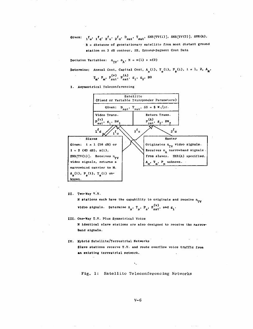
Given: I ' 1 id' 2f u 2d , Dsat Tsat, SNR[TV(1)], SNR[TV(2)], SNR(A),

R = distance of geostationary satellite from most distant ground

station on 3 dB contour, SS, Ground-Segment Cost Data

Decision Variables: nT, nA , N = n(l) + n(2)

Determine: Annual Cost, Capital Cost, As(i), Ts(i), Ps(i), i = 1, 2, Amp

(v) (A)Tm' Pm P sat' sat' g1 ' g2 ' BO

I. Asymmetrical Teleconferencing

Satellite(Fixed or Variable Transponder Parameters)

Given: Dsa , T sa t , SS = $ W./yr.

Given: i = 1 (56 dB) or Originates nrV video signals.

=2(43 dB), n(i), Receives nA narrowband signals .

SNR[TV(i)]. Receives nTV from slaves. SNR(A) specified.

video signals, returns a A , T , P unknown.

narrowband carrier to M.

A (i), P (i), T (i) un-

known.

II. Two-Way T.V.

N stations each have the capability to originate and receive nTV

(v)video signals. Determine A, Ts, P, P sat and g .

III. One-Way T.V. Plus Symmetrical Voice

N identical slave stations are also designed to receive the narrow-

band signals.

IV. Hybrid Satellite/Terrestrial Networks

Slave stations receive T.V. and route overflow voice traffic from

an existing terrestrial network.

Fig. 1: Satellite Teleconferencing Networks

V-6

a factor of 3 increases the cost by roughly qT3. This conclu-sion is based on the assumption that the total number of sta-tions and the channel capacity are constant.

6. There are significant economies of scale. When there is onevideo-origination station and N slave stations which receivethe video and return the narrowband information to the video-origination station, the total capital cost per station fallsapproximately as NN.

7. Until the spectrum must be reused*, the marginal cost of addingvideo channels is constant when the satellite parameters arefixed and decreases when the satellite parameters are variable.When the spectrum must be reused, the ground-segment costsincrease significantly, increasing the marginal cost.

8. The availability of directive antennas and larger amounts ofRF power on a communication satellite - to the extent thatthey reduce the cost-per-watt-per-year of satellite power -will have a significant bearing on the configuration of theminimum-cost network. If SS is the annual cost per watt ofsatellite power, the annual cost of the network rises approx-imately as %1SS.

9. The gross system parameters of the minimum-cost network, ATs, Ps, Am, Tm, Pm, p(v), and BO, are quite sensitive tovariations in N, nTV , and nA. Because these demand indica-tors are unlikely to be known with precision, the supplierprobably would seek a compromise solution rather than attemptto minimize his annual cost.

10. Frequency-division-multiple-access appears to be less costlythan time-division-multiple-access for the master/slave net-work configurations that we have considered.

In sections C and D, we shall consider satellite teleconferencing un-

der two settings: when the transponders are fixed and only the ground

segment may be optimized and when both the ground and space segments are

variable. We consider both digital feedback and voice feedback in the

case studies. Two classes of slave stations are considered in Section

C.2: otherwise the slave stations are assumed to be identical.

The channel capacity of the allocated frequency band may be increased bya factor of two by using orthogonally polarized beams. We have assumedthat two antennas and two pre-amps will be used at each slave station inthis event. V-7

Network configurations having greater symmetry are considered in

Section E. Numerical results are obtained for two-way video telecon-

ferencing systems; and the case in which the N slave stations also

serve as transit centers for a telephone distribution network is out-

lined. The analytical tools used throughout this report are developed

in Section B.

V-8

2. Review of Literature

Low-cost communications are a common international concern. As

would be expected, numerous authors have addressed themselves to the

problem of determining the minimum-cost network for a particular set of

requirements. We gratefully acknowledge the inspiration we derived from

the previous contributions of Lutzl, Chakraborty2 , McClure 3 , Dickinson4

and Talyzin, Kantor, Maryakin, and Payansky5 ,6 ,7. It perhaps would be

appropriate at this time to indicate the point of departure of our work

from these previous developments.

Lutz was the first to clarify the methodology required to quantify

the ground/space tradeoffs in a satellite communications network. He

simplified the complex relationship between the ground-station parameters,

(D,T,P), the space-segment charges of the satellite, and the performance

characteristics of the satellite transponder by expanding the cost equa-

tion into a Taylor series and restricting his attention to only the

first-order terms. Unfortunately, he did not first attempt to optimize

the satellite and the ground-stations as a function of the required

area of coverage, channel capacity, and signal-quality-constraints.

That is, neither the satellite characteristics, space-segment charge,

or ground-station parameters were allowed to vary. Consequently, the

system as a whole generally was distinctly sub-optimal; and, not unex-

pectedly, Lutz came to the disappointing conclusion that small ground

stations are "expensive bargains."

Previous attempts to optimize the ground and space segments often

have been undermined by unduly restrictive assumptions.* In particular,

the noise budget should not be partitioned a priori. This result

should be an outcome, rather than a premise, of an optimization study.

The determination of the least-cost allocation of the allowed noise in

the system between the satellite, master station, and slave stations is

the central issue in the optimization procedures to be described.

See for example, the conclusions of the Interim Meeting of Study GroupW of the CCIR: "A Comparative Study of Possible Methods of Modulationand Multiple Access (for Multi-Channel Telephony)," Geneva, October1968.

V-9

The richest source of literature pertaining to ground/space tradeoffs

derives from studies of the Intelsat system. The usual problem consider-

ed in the Intelsat literature is to determine the satellite parameters

which maximize the (voice) channel capacity to a link between two stan-

dard stations. References 2 and 3 provide excellent treatments of this

problem.

Our problem is significantly different: the traffic pattern is in-

herently asymmetrical, and neither the space nor the ground-segment

parameters have been fixed a priori. For a fixed traffic pattern, the

problem is to specify these parameters so as to minimize the annual cost.

The two-way problem is more difficult to analyze than the one-way

problem. In the receive-only case, to achieve a specified receiver

sensitivity (as measured by the G/T ratio), there is usually a unique

combination of G and T which minimizes the total cost. 4 Similarly, for

a specified value of uplink EIRP (equal to the product of antenna gain

and uplink RF power), generally there is a unique combination of G and

P which minimizes the cost of providing this EIRP. When one antenna is

to be used both to receive and to transmit, these problems must be con-

sidered jointly. We shall consider techniques to deal with the effects

of coupling in the sections to follow.

The Russian papers5,6, 7 are similar in spirit to our own analy-

sis: they too are concerned with providing economical telecommunications

to the small user. It is conceivable that they used the same analytical

tools, although this is not evident from the brief published excerpts of

their work or from their references. Our thinking was shaped most prom-

inently by the Comsat references. 2 ,3

B. Analytical Framework

1. Cost Equation

Suppose that there are N identical slave stations in the network,

each of which receives nTV video channels and require a total of nA re-

turn channels on the satellite. Define:

C t = total annual cost of the system;

V-10

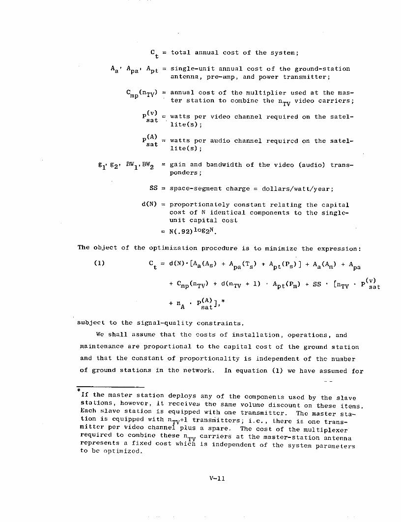
Ct = total annual cost of the system;

Aa' Apa' Apt = single-unit annual cost of the ground-stationantenna, pre-amp, and power transmitter;

Cmp(nTV) = annual cost of the multiplier used at the mas-ter station to combine the nTV video carriers;

P(v) = watts per video channel required on the satel-satlite(s);

(A) = watts per audio channel required on the satel-sat lite(s);

gl1 g2 ' BW1 1BW2 = gain and bandwidth of the video (audio) trans-ponders;

SS = space-segment charge = dollars/watt/year;

d(N) = proportionately constant relating the capitalcost of N identical components to the single-unit capital cost

= N(.92)log2 N .

The object of the optimization procedure is to minimize the expression:

(1) Ct = d(N)-[Aa(As) + Apa(Ts) + Apt(Ps) ] + Aa(Am) + Apa

(v)+ Cmp(nTV) + d(nTV + 1) • Apt(Pm) + SS * [nTV ' sat

+ nA * p(A)] *A sat '

subject to the signal-quality constraints.

We shall assume that the costs of installation, operations, and

maintenance are proportional to the capital cost of the ground station

and that the constant of proportionality is independent of the number

of ground stations in the network. In equation (1) we have assumed for

If the master station deploys any of the components used by the slavestations, however, it receives the same volume discount on these items.Each slave station is equipped with one transmitter. The master sta-tion is equipped with nTV+l transmitters; i.e., there is one trans-mitter per video channel plus a spare. The cost of the multiplexerrequired to combine these nTV carriers at the master-station antennarepresents a fixed cost which is independent of the system parametersto be optimized.

V-11

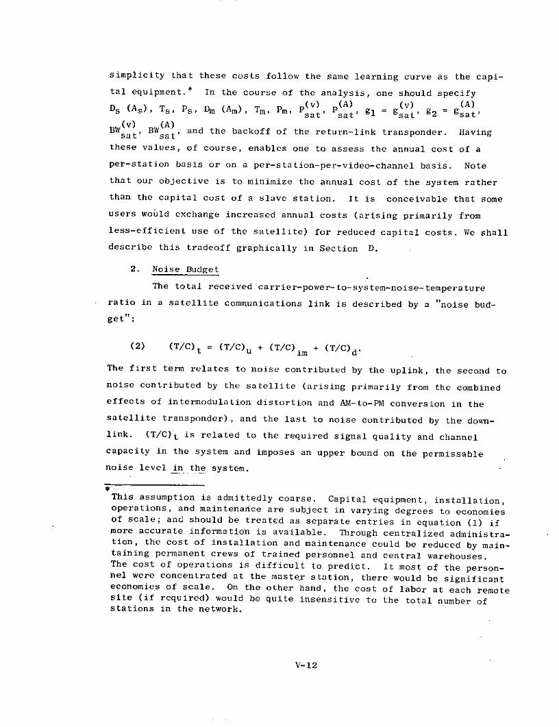
simplicity that these costs follow the same learning curve as the capi-

tal equipment.* In the course of the analysis, one should specify

Ds (As), Ts, Ps, Dm (Am), Tm, Pm, p(V) P(A) g(V) (A)sat' sat' gl = sat' g2 =gsat'(v) (A)BW (vsat , BWsat' and the backoff of the return-link transponder. Having

these values, of course, enables one to assess the annual cost of a

per-station basis or on a per-station-per-video-channel basis. Note

that our objective is to minimize the annual cost of the system rather

than the capital cost of a slave station. It is conceivable that some

users would exchange increased annual costs (arising primarily from

less-efficient use of the satellite) for reduced capital costs. We shall

describe this tradeoff graphically in Section D.

2. Noise Budget

The total received carrier-power-to-system-noise-temperature

ratio in a satellite communications link is described by a "noise bud-

get":

(2) (T/C)t = (T/C)u + (T/C)im + (T/C)d"

The first term relates to noise contributed by the uplink, the second to

noise contributed by the satellite (arising primarily from the combined

effects of intermodulation distortion and AM-to-PM conversion in the

satellite transponder), and the last to noise contributed by the down-

link. (T/C)t is related to the required signal quality and channel

capacity in the system and imposes an upper bound on the permissable

noise level in the system.

This assumption is admittedly coarse. Capital equipment, installation,operations, and maintenance are subject in varying degrees to economiesof scale; and should be treated as separate entries in equation (1) ifmore accurate information is available. Through centralized administra-tion, the cost of installation and maintenance could be reduced by main-taining permanent crews of trained personnel and central warehouses.The cost of operations is difficult to predict. It most of the person-nel were concentrated at the master station, there would be significanteconomies of scale. On the other hand, the cost of labor at each remotesite (if required) would be quite insensitive to the total number ofstations in the network.

V-12

The total system cost, Ct, is critically independent on how the noise

budgets for the video and return links are allocated. This decision is

not an arbitrary matter: for each alternative partitioning of the two

noise budgets there is an associated cost, which we shall examine care-

fully in the sections to follow. Increasing the required signal quality

or the channel capacity is tantamount to reducing the allowable noise

level in the system, which entails an increase in the total cost.

We shall assume both for the uplink and the downlink that thermal

noise dominates.* Define (T/C)q = (/C) t - (T/C)im. Then equation (2)

becomes:

(3) (T/C)q = (T/C)u + (T/C)d'

Suppose (C/T)u = x(C/T)d. Then each of these terms may be related to

quasi signal-quality constraint; (C/T)q = (C/T)U = (1 + x)'(C/T)q

(C/T)d = (1 + x-1)(C/T)q

For each partitioning of the audio and video noise budgets [represented,

(v) (v) (A) (A)say, by (C/T)u = x-(C/T) d and (C/T) = y.(C/T)d ], a corresponding

set of ground and space-segment parameters may be determined which

minimizes the annual cost for the particular value of the couplet (x,y).

One then searches over a range of partitionings to obtain the global

minimum. For TV-only operation, one need only search over x.

3. Cost Data

Only the capital cost of the antenna, pre-amp, power transmitter,

and master-station multiplexer is considered explicitly in our analysis

of ground-segment costs.** The cost of installation, operations, and

maintenance is assumed to be proportional to these capital costs. Let

Ca [A(D)] be the capital cost of an antenna of effective area A feet2

The other sources of noise, such as earth-station, non-linearities, in-terference from terrestrial systems which share the spectrum, etc.,have been lumped with thermal noise to obtain an estimated value of"total system noise."

Modem costs should have been considered, but insufficient data wasavailable. A more complete description of the cost data obtained bythe Stanford teleconferencing group may be found in Chapter 3.

V-13

(and diameter D feet), Cpa (T) be the capital cost of a pre-amp having

noise temperature T, and Cpt(P) be the capital cost of a power transmit-

ter having an RF output power of P watts. The cost of installation,

which represents a capital investment, is assumed to consist of two com-

ponents:

1. Installation and Alignment of Antenna

S.15Ca[A(D)], D s 12'

Installation Cost = .20Ca[A(D)], 12'<D- 40'

.30Ca[A(D)], D >40'

2. Water, Power, Roads, and Miscellaneous Equipment

Cost = .15[Ca (A) + Cpa (T) + Cpt (P)].

The cost of operations and maintenance, which are treated as annual costs,

depends on the particular components employed. Our cost estimates are

categorized below:

1. Antenna .05Ca[A(D)], D-<12'

O&M Cost .075Ca[A(D)], 12'< D S40'

15Ca[A(D)], D >40'

2. Pre-amp

.25C pa(T), T<700 K (Cooled parametric amplifier

pa

.15Cpa(T) 700 K< T< 3000 K (uncooled paramp)O&M Cost

.05Cpa(T), T _300 0 K (solid-state or mixer

pre-amp)

3. Power Transmitter

.05Cpt(P), P<30 w (solid state)

O&M Cost

.20Cpt(P), P >30 w (klystron or TWT)

4. Miscellaneous

0&M Cost . 0[Ca (A) + Cpa(T) + Cpt(P)]

V-14

We have assumed that the ground stations are amortized over 10 years at

an interest rate of 10%. Thus, the annual payments on capital invest-

ments amount to approximately 16.2% of the first cost. To these interest

payments must be added the estimated cost of operations and maintenance.

The single-unit annual cost associated with use of the various components

by Aa(A), Apa(T), and Apt(P).

The small ground stations under consideration tend to be power limi-

ted rather than bandwidth limited. Consequently, we have assumed their

space-segment charges are assessed on the basis of average power consump-

tion on the satellite and are not related to their consumption of band-

width.

The annual cost of a satellite transponder is assumed to be a linear

function of the RF output power of that transponder; it is assumed to

be independent of the power gain or the bandwidth. One selects that

satellite which provides the most watts per dollar as described in Chap-

ter IV.

Use of the geostationary orbit is assumed to be free of charge.

This assumption will have to be revised if the demand for low-cost

ground stations, which make relatively inefficient use of the geostation-

ary spectrum, overruns the supply of orbital slots. We do not feel that

this circumstance is likely in the foreseeable future; but steps not to

insure conservation of this scarce resource--without stiffling its

development--would not be unwarranted. A combination of political, legal,

and technical factors would have to be included in any meaningful analy-

sis of the economic value of this resource. If the cost could be expres-

sed in terms of $/degree of orbital arc/Hz of RF spectrum/year, this fac-

tor could easily be incorporated into equation (1), which we have used

as the figure of merit in comparing alternative system designs. Unfor-

tunately, the complex topic of orbital conservation is beyond the scope

of our present analysis.

The system noise temperature, T, and the uplink RF power, P, have

been restricted to a discrete range of values; the antenna diameter has

been allowed to range over a continuum. Were the diameter restricted

to a discrete set, it would be necessary to replace the differential-

calculus procedures to be described with exhaustive search techniques.

V-15

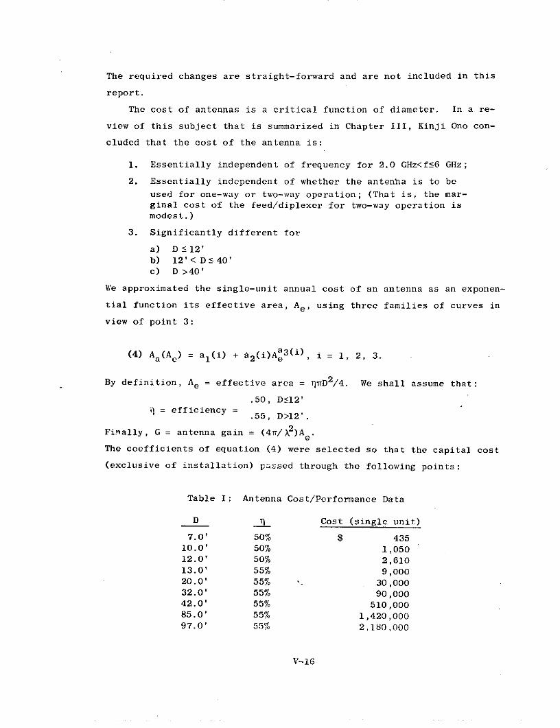
The required changes are straight-forward and are not included in this

report.

The cost of antennas is a critical function of diameter. In a re-

view of this subject that is summarized in Chapter III, Kinji Ono con-

cluded that the cost of the antenna is:

1. Essentially independent of frequency for 2.0 GHz<fS6 GHz;

2. Essentially independent of whether the antenha is to be

used for one-way or two-way operation; (That is, the mar-ginal cost of the feed/diplexer for two-way operation ismodest.)

3. Significantly different for

a) D 12'b) 12'< D:540'c) D >40'

We approximated the single-unit annual cost of an antenna as an exponen-

tial function its effective area, Ae, using three families of curves in

view of point 3:

(4) Aa(Ae) = al(i) + a2 (i)Aa3(i), i = 1, 2, 3.

By definition, Ae = effective area = TD2/4. We shall assume that:

.50, Dfl2'= efficiency =

.55, D>12'.

Finally, G = antenna gain = (4n/X2)Ae

The coefficients of equation (4) were selected so that the capital cost

(exclusive of installation) passed through the following points:

Table I: Antenna Cost/Performance Data

D 1 Cost (single unit)

7.0' 50% $ 43510.0' 50% 1,05012.0' 50% 2,61013.0' 55% 9,00020.0' 55% -- 30,00032.0' 55% 90,00042.0' 55% 510,00085.0' 55% 1,420,00097.0' 55% 2,180,000

V-16

Above 12', the manufacturing costs are much higher. Below 12', the

techniques developed by Janky and Taggart of Stanford University are

applicable.8 These small antennas are now commercially available.

Six pre-amplifier configurations have been considered:

1. A parametric amplifier, the first stages of which arehelium-vapor cooled. (Amplifier noise temperature,Tn 200 K; system noise temperature, T,= 450 K).

2. A parametric amplifier, the first stages of which are liquid-nitrogen cooled; TnY 400 K, T:680 K.

3. Uncooled, two-stage parametric amplifier, Tn 900 K, T ~1250 K.

4. An uncooled, single-stage parametric amplifier, T 1 8 0 o K,T : 228 0 K.

5. A solid-state amplifier, Tn=3200 K, Ta3850 K.

6. A mixer front end, Tnl 1 50 0 K, Ta1565 K.

The losses arising from the antenna, feed, and wave guides have been

assumed to range from 250 K to 650 K, depending on the cost of the

antenna/feed design.

Eleven values of uplink RF power were considered, ranging from .1

watt to 10 kilowatts. A table of values and the associated single-unit

costs follows. Included is the estimated site cost of the antenna and

a column relating the per-unit cost of N identical items to the single-

unit cost assuming that cost = (.9 2 )log2 N units. Tsat was fixed through-

out at 1600 Ko in the case studies.

4. State Equations

Let us now relate the terms of equations (2) to the space and

ground-segment parameters. Define

f = input flux density required to saturate the satel-x lite transponder = watts/feet2 ;

fxr = 4R 2 , where R is the distance of the geostationarysatellite from the most distant ground station onthe 3 dB beam edge;

Psat = RF output power of the satellite transponder;

V-17

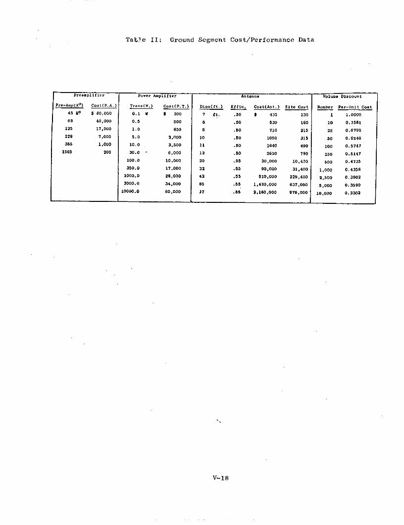
Tabl.e II: Ground Segment Cost/Performance Data

Preamplifier Power Amplifier Antenna Volume Discount

Pre-Amp(Ko) Cost(P.A.) Trans(W.) Cost(P.T.) Diam(ft.) Effic. Cost(Ant.) Site Cost Number Per-Unit Cost

45 Ko $ 80,000 0.1 W $ 200 7 ft. .50 $ 435 130 1 1.0000

68 40,000 0.5 500 8 .50 530 160 10 0.7581

125 17,000 1.0 850 9 .50 710 215 25 0.6790

228 7,000 5.0 2,000 10 .50 1050 315 50 0.6246

385 1,000 10.0 3,500 11 .50 1640 490 100 0.5747

1565 200 30.0 6,000 12 .50 2610 780 250 0.5147

100.0 10,000 20 .55 30,000 10,470 500 0.4735

350.0 17,000 32 .55 90,000 31,400 1,000 0.4356

1000.0 28,000 42 .55 510,000 229,400 2,500 0.3902

3000.0 34,000 85 .55 1,420,000 637,000 5,000 0.3590

10000.0 60,000 J7 .55 2,180,000 978,000 10,000 0.3302

V-18

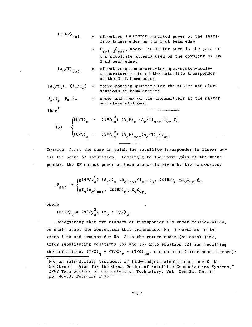
(EIRP)sat = effective isotropic radiated power of the satel-

lite transponder on the 3 dB beam edge

= P sat G where the latter term is the gain orsat d sat'

the satellite antenna used on the downlink at the3 dB beam edge;

(Ae/T) = effective-antenna-area-to-input-system-noise-temperature ratio of the satellite transponderat the 3 dB beam edge;

(As/Ts), (Am/Tm) = corresponding quantity for the master and slavestations at beam center;

Ps s' Pm, 2m = power and loss of the transmitters at the masterand slave stations.

Then

(C/T) = (4 /K ) (A P) (A /T) /'f uu u e u e sat xr u(5)

(C/T) = (4 / ) (A P) (A e/T) /fxd d e sate d xr

Consider first the case in which the satellite transponder is linear un-

til the point of saturation. Letting g be the power gain of the trans-

ponder, the RF output power at beam center is given by the expression:

g(4r/k ) (A P) (Ae)sat /fxr ' (EIRP) 5f f uSsat = g u e u e sat xr u u x xr u

gf (A) ,(EIRP) >ffx e sat u x xr,

where

(EIRP) (4/%/2 ) (A P/ ) uu u e u

Recognizing that two classes of transponder are under consideration,

we shall adopt the convention that transponder No. 1 pertains to the

video link and transponder No. 2 to the return-audio (or data) link.

After substituting equations (5) and (6) into equation (2) and recalling

the definition, (T/C) = (T/C)t - (T/C)im , one obtains (after some algebra):

For an introductory treatment of link-budget calculations, see G. M.Northrup: "Aids for the Gross Design of Satellite Communication Systems,"IEEE Transactions on Communication Technology, Vol. Com-14, No. 1,pp. 46-56, February 1966.

V-19

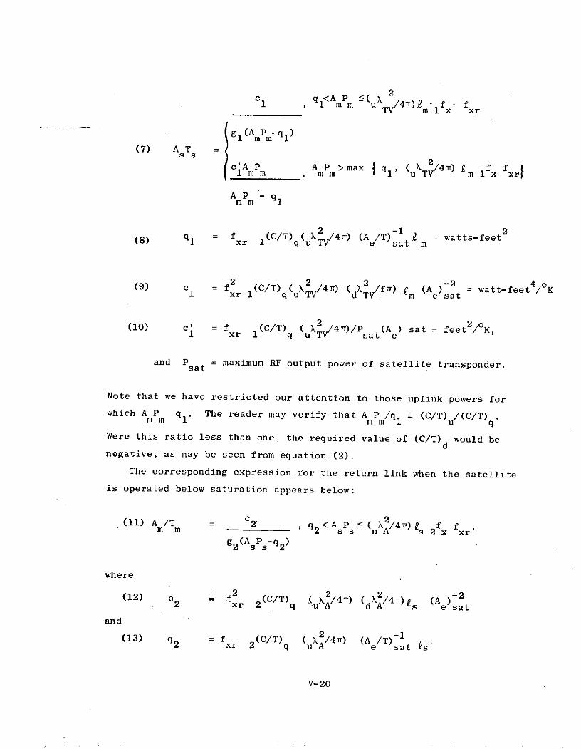
C q <APm ( ku /4T) f * fu TV mi1x xr

(g1 (A P q 1)(7) A T =

S cAP m AP >max iq (uT T4 ) f fx1 mm m 1 u TV m x xr

AP - q

2 -1 2q = f (C/T) ( V/4r) (A /T) 9 = watts-feet(8) 1 xr 1 q u T e sat

(9) c = f2 (C/T) (u2 /4) ( X f2 )f (A )a2t = watt-feet4 /K1 xr 1 quTV d T m e sat

2 2/°K,(10) c' = f (C/T) 2 /4r)/Psat (A ) sat = feet / K,1 xr 1 q u TV sate

and Psat = maximum RF output power of satellite transponder.

Note that we have restricted our attention to those uplink powers for

which A P ql. The reader may verify that A P /q = (C/T) /(C/T) .mm mm u q

Were this ratio less than one, the required value of (C/T)d would be

negative, as may be seen from equation (2).

The corresponding expression for the return link when the satellite

is operated below saturation appears below:

(11) A /T = c2 q 2<AP X/4r) fm m 2 Pss u A s 2 x xr'

g2 (AsPs-q 2

where

(12) c 2 = 2 (C/T) (uk /4r ) (d 2 /4T) s (Ae sat

and

(13) q = f (C/T) ( X2/4 ) (A /T) -2 xr 2 q uA e sat 2s

V-20

m', the power loss incurred in the video origination station, is a

function of the number of video carriers multiplexed at the master sta-

tion and is tabulated in Table III. 2s, the power loss of a slave sta-

tion, is assumed to be 1.0 dB. Equations (7) through (13) establish

the physical relationships between the ground and space-segment parame-

ters which must be satisfied if the signal-quality constraints (which

are related to (C/T) and (C/T) are to be met.1 q 2 q

Consider now the case in which the satellite employs a hard limiter

and/or automatic-gain control. Hard limiters have been employed exten-

sively on communications satellites to insure that the limited available

output power is fully utilized. The ideal hard limiter provides maximum

output power however small the input power may be. Alternatively, auto-

matic-gain control may be used to place the operating point at some

specified value below the saturation point. This technique is attractive

when multiple carriers are to access the transponder simultaneously, and

it is necessary to reduce the intermodulation distortion generated in the

transponder. Denote the nominal operating point, whether it be at satu-

ration or some lesser value, by Psat. We shall begin as before with

equation (2). As defined, the numerator in the term (C/T)d pertains to

that fraction of the satellite output power containing the signal. Denote

this fraction by C and define Psat = C + N and let L = C/P sat It fol-

lows that L = 1 + N/C. If B is the RF bandwidth of the transponder and

k is Boltzmann's constant, then

N/C = kB[(T/C)u + (T/C)im].

-1By definition L (C/T)d = (EIRP)sat (A /T) d/fxr

Substituting into equation (2), one ultimately obtains the expression:

(14) A /T c AP(c +c /AP), AP q', (XU2 /4) fs 11 m m 12 13 m m m ' u TV ml x xrAP -'mm q

where

V-21

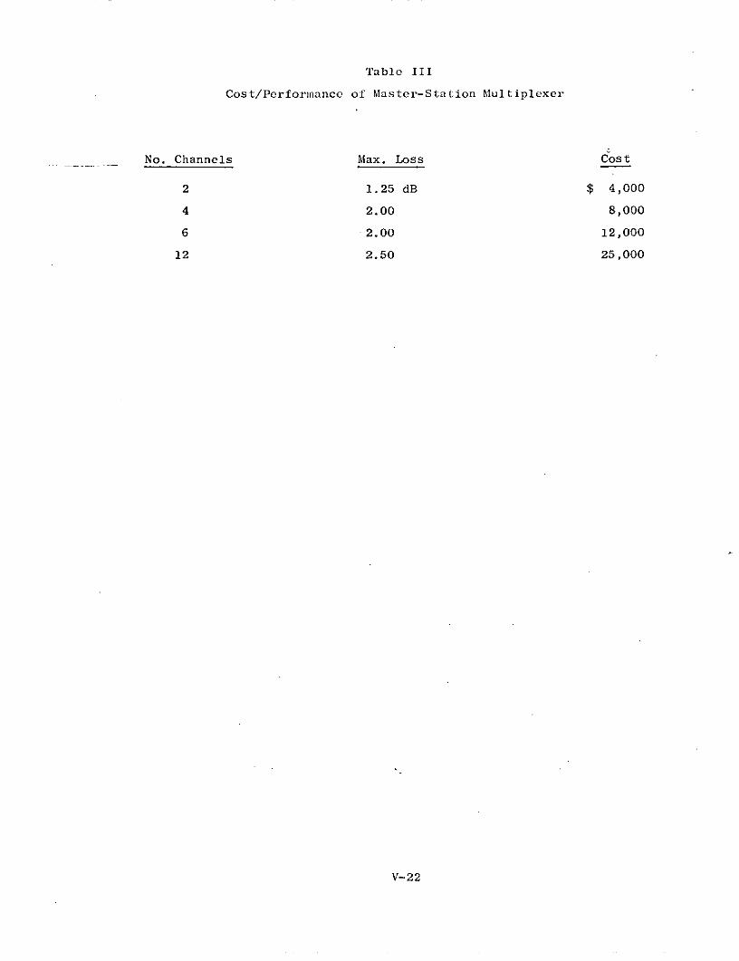
Table III

Cost/Perforinance of Master-Station Multiplexer

No. Channels Max. Loss Cost

2 1.25 dB $ 4,000

4 2.00 8,000

6 2.00 12,000

12 2.50 25,000

V-22

(15) C1 1 = (C/ ( t xr/ { h (C/T) t/(C/T) im], (EIRP) sat}

-1(16) c = 1 + kB(C/T)- ,

12 im'

(17) c 1 3 =kBf 2 ( O4) (A /T) ,and13 xr uTV e sat

2 -1(18) q (C/T)tfxr(u / 4 Tr) (A /T) /[1- (C/T) /(C/T)im](18)ruT e sat 1 t i

Corresponding expressions may be written for the return link, where one

replaces 1(C/T)t with 2(C/T)t, m with s, and Psat and 'TV with the

expressions appropriate for the return link.

When only one carrier accesses the transponder, intermodulation dis-

tortion is negligible; and c12 l, c 11c', and q' q l , where c' and ql

are defined by equations (9) and (7).

5. Signal-Quality Constraints

To complete the description of the coefficients' defined above,

it is necessary to relate 1(C/T)t and 2(C/T)q to the specified quality

standards for the video and audio links.

Consider first the video link. Our design objective was to achieve

at the receiver output a peak-to-peak-signal-to-weighted-noise-power

ratio of either 43.0 dB or 56.0 at the 3 dB beam edge. From the FM

equation,

(19) (SNR) = 6[(B/2f ) -1] 2 (C/N) (B/f )km m p

Equation (19) is based on the assumption that the RF bandwidth isgiven by Carson's rule, or B = 2fm(m+l). Recent experimental evidencesuggests that the RF bandwidth allocated per video signal need not ex-ceed the peak-to-peak frequency deviation, or a bandwidth of 2f -mwould suffice. Obviously these results, if confirmed, should be usedin dimensioning future FM video systems. For detials see "BreadboardDesign and System Analysis for the ATS-F TRUST Experiment Small GroundStation," Communication R&D Branch, Goddard Space Flight Center, NASA,Greenbelt, Md., September 1971, pp. 2-48 through 2-68.

V-23

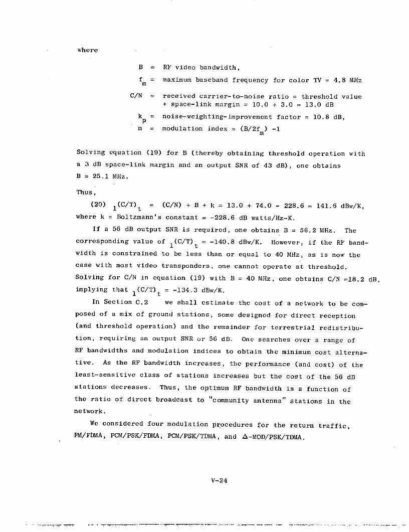
where

B = RF video bandwidth,

f = maximum baseband frequency for color TV = 4.8 MHz

C/N = received carrier-to-noise ratio = threshold value+ space-link margin = 10.0 + 3.0 = 13.0 dB

k = noise-weighting-improvement factor = 10.8 dB,p

m = modulation index = (B/2f) -1m

Solving equation (19) for B (thereby obtaining threshold operation with

a 3 dB space-link margin and an output SNR of 43 dB), one obtains

B = 25.1 MHz.

Thus,

(20) 1(C/T)t = (C/N) + B + k = 13.0 + 74.0 - 228.6 = 141.6 dBw/K,

where k = Boltzmann's constant = -228.6 dB watts/Hz-K.

If a 56 dB output SNR is required, one obtains B = 56.2 MHz. The

corresponding value of 1(C/T) t = -140.8 dBw/K. However, if the RF band-

width is constrained to be less than or equal to 40 MHz, as is now the

case with most video transponders, one cannot operate at threshold.

Solving for C/N in equation (19) with B = 40 MHz, one obtains C/N =18.2 dB,

implying that 1(C/T)t = -134.3 dBw/K.

In Section C.2 we shall estimate the cost of a network to be com-

posed of a mix of ground stations, some designed for direct reception

(and threshold operation) and the remainder for terrestrial redistribu-

tion, requiring an output SNR or 56 dB. One searches over a range of

RF bandwidths and modulation indices to obtain the minimum cost alterna-

tive. As the RF bandwidth increases, the performance (and cost) of the

least-sensitive class of stations increases but the cost of the 56 dB

stations decreases. Thus, the optimum RF bandwidth is a function of

the ratio of direct broadcast to "community antenna" stations in the

network.

We considered four modulation procedures for the return traffic,

FM/FDMA, PCM/PSK/FDMA, PCM/PSK/TDMA, and A-MOD/PSK/TDMA.

V-24

The design goal was to achieve an output signal-to-noise ratio of

43 dB at the headend. From the FM equation,9

(21) (SNR) = 3m2 (C/N) (B/f ) k'm p

where the terms are defined as before with the exception of the fact that

we are concerned with rms signal power and that k' is the peak-to-average, p

factor for single-channel-per-carrier voice. Choosing k' = 13.0 dBP 10

insures that the peak values will not be clipped more than 1% of the time.

Again using a threshold value of 10.0 dB with a 3.0 dB space-link margin,

we have C/N 2 13.0 dB. Solving equation (21) for m, one obtains m = 14.2,

implying that B 2(14.2 + 1) (3400 Hz) ~ 100 kHz.

Thus,

(22) 2(C/T) t = 13.0 + 50.0 - 228.6 = 166.6 dBw/K

Consider now PCM/PSK. Operation is said to be bandwidth limited if

the following inequality, expressed in dB, is satisfied:

(23) B + log 2 L1 - R 5 (C/kT) - (E/No ) 2 MR

where (C/kT)t is the total carrier-power-to-noise-density ratio of the

communications link, as given by equation (2). Otherwise, the system is

said to be power limited. Prior to the advent of high-power TWT's and

directive antennas, virtually all satellite communications networks

tended to be power limited. Most stations in the Intelsat network are

now bandwidth limited, and the tariff structure reflects the need to

conserve bandwidth, which is relatively scarce. As mentioned previously,

the small stations that we are considering tend to be power limited; and

they are not charged for their use of bandwidth. The new terms introduced

in inequality (23) are defined as follows:

We have not assumed that syllabic companders or pre-emphasis will beused. These features would reduce k and should be studied. For adiscussion of state-of-the art techniques, see P.M. Boudrean and N.G.Davies, "Modulation and Speech Processing for Single-Channel-per-CarrierSatellite Communications," 1971 International Conference on Communications.

V-25

R = required bit rate

L = number of levels in the PSK code

E/N o = received-energy-to-noise-power-density ratio

2 = implementation loss in the PSK modem

M = space-link margin

For voice, it is considered advisable to use 7-level PCM (with an eighth

level for syncronization) and to sample at 8 kbps. Thus, R = 64.0 kbps

= 48.1 dB-Hz. Typical numbers employed in a four-phase PSK system4

are: = 2.3 dB, M = 3.0 dB, L = 4, and E/N o = 8.4 dB-Hz 2 (which provides

a bit-error-rate of 1 in 104). The required carrier-power-to-system-

noise-temperature ratio is then:

(24) 2(C/T)t = (E/N o ) + 2+ R + M + k = 8.4 + 2.3 + 58.1 + 3.0

- 228.6 = -166.8 dBw/K.

On this basis, at least, there is little to distinguish between FM and

PCM/PSK. At the present time, however, modem costs are much lower for

FM. The picture may change in the future, which would be desirable in

view of the flexibility offered by PCM/PSK in our case studies of digital

feedback, although we would recommend using F for voice-feedback systems

comtemplated over the near term.

A-MOD/PSK appears to offer significant power savings, although its

merit relative to PCM/PSK remains controversial.11 One may transmit at

half the bit rate at a bit-error-rate of 1 in 103 (rather than 1 in 104),

resulting in a power savings of approximately 4.0 dB.1 2 That is, for

A-MOD/PSK, 2(C/T)t = 170.8 dBw/K for voice quality comparable to 43 dB

in the FM case.

6. Intermodulation Distortion

As a satellite transponder is driven toward saturation, opera-

tion becomes increasingly nonlinear and intermodulation distortion in-

creases. The extent to which a transponder is operated below saturation

is known as input backoff, which in dB is defined by equation (25):

V-26

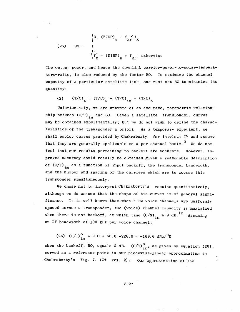
0, (EIRP) - f !=fS(ERP)u xr x

(25) BO =

- (EIRP) + f xr otherwise

The output power, and hence the downlink carrier-power-to-noise-tempera-

ture-ratio, is also reduced by the factor BO. To maximize the channel

capacity of a particular satellite link, one must set BO to minimize the

quantity:

(2) (T/C) = (T/C) + (T/C). + (T/C)dt u im

Unfortunately, we are unaware of an accurate, parametric relation-

ship between (C/T). and BO. Given a satellite transponder, curves

may be obtained experimentally; but we do not wish to define the charac-

teristics of the transponder a priori. As a temporary expedient, we

shall employ curves provided by Chakraborty for Intelsat IV and assume

that they are generally applicable on a per-channel basis. 2 We do not

feel that our results pertaining to backoff are accurate. However, im-

proved accuracy could readily be obtained given a reasonable description

of (C/T). as a function of input backoff, the transponder bandwidth,Im

and the number and spacing of the carriers which are to access this

transponder simultaneously.

We chose not to interpret Chakraborty's results quantitatively,

although we do assume that the shape of his curves is of general signi-

ficance. It is well known that when N FM voice channels are uniformly

spaced across a transponder, the (voice) channel capacity is maximized13

when there is not backoff, at which time (C/N) 9 dB.13 Assumingim

an RF bandwidth of 100 kHz per voice channel,

(26) (C/T)o = 9.0 + 50.0 -228.6 = -169.6 dBw/oKim

when the backoff, BO, equals 0 dB. (C/T)o , as given by equation (26),imserved as a reference point in our piecewise-linear approximation to

Chakraborty's Fig. 7. (Cf: ref. 2). Our approximation of the

V-27

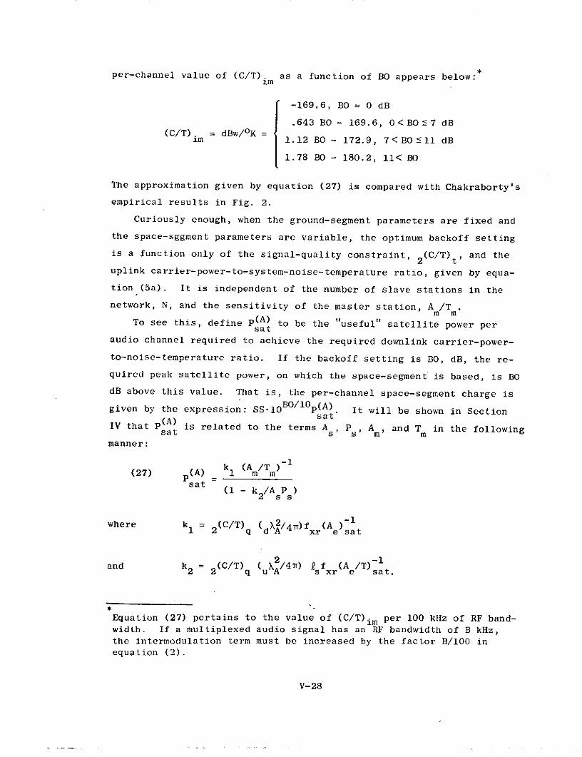
per-channel value of (C/T). as a function of BO appears below:im

-169.6, BO = 0 dB

.643 BO - 169.6, 0< BO 7 dB(C/T) = dBw/oK(C/T) im 1.12 BO - 172.9, 7<BO 11 dB

1.78 BO - 180.2, 11< BO

The approximation given by equation (27) is compared with Chakraborty's

empirical results in Fig. 2.

Curiously enough, when the ground-segment parameters are fixed and

the space-sggment parameters are variable, the optimum backoff setting

is a function only of the signal-quality constraint, 2(C/T)t, and the

uplink carrier-power-to-system-noise-temperature ratio, given by equa-

tion (5a). It is independent of the number of slave stations in the

network, N, and the sensitivity of the master station, A /T .m mTo see this, define p(A) to be the "useful" satellite power persat

audio channel required to achieve the required downlink carrier-power-

to-noise-temperature ratio. If the backoff setting is BO, dB, the re-

quired peak satellite power, on which the space-segment is based, is BO

dB above this value. That is, the per-channel space-segment charge is

given by the expression: SS10 BO/10p(A) . It will be shown in Sectionsat

IV that P sat is related to the terms A Ps, Am, and T in the following

manner:

(27) (A) k (A1 m/T msat

(1 - k /AsP )2 ss

2 - lwhere k = (C/T) (X2/ 4Tr)f (A )

1 2 q dA xr e sat

2 -1and k = (C/T) ( X/4r) R f (A /T)-2 2 q uA s xr e sat.

Equation (27) pertains to the value of (C/T)im per 100 kHz of RF band-width. If a multiplexed audio signal has an RF bandwidth of B kHz,the intermodulation term must be increased by the factor B/100 inequation (2).

V-28

- 141.7

TWT COMPRESSION NONLINEARITY + AM TO PM CONVERSION EFFEC

- 145.7

- 149.7

LCJ

- 153.7

-o

- 0

- 161.7

- 165.7

- 169.7

- 0

I, I-

- 173.7 I10- 165.7 I 4 0

TRANSPONDER FINAL TWT INPUT BACKOFF

Fig. 2: (C/T). vs. Backofflm

V-29

(C/T) may be related to BO using equation (27):2 q

(C/T)

(C/T) =2 q 1 - 2 (C/T)t exp[.2303(b1 BO + b2)]

It follows that the space-segment charge is proportional to the expres-

sion:

(28) (A) 1 exp(.2303BO)(28) P =

sat 1 - c 2 - c 3 exp(-.2303b 1 BO)

where

- 2 -1c (C/T) (A /T )- ( 2/ 4n)f (A )at

1 2 t m m dXA xr e sat,

-1 2 -1c2 = (C/T) (AsP ) ( X/4r) xf (A /T)2 2 t s uA s xr e sat

= (C/T) t/(C/T) <1,

and

c 3 = 2(C/T)texp [-.2303 b2]

Differentiating (28) to minimize the space-segment charge, one obtains:

(29) BO(dB) = (C/T) -b2 + 101og 1 0 I+bl

For the asymmetrical links under consideration, the ratio of total

noise to uplink noise ranges from 4 to 18 dB. To obtain a 43 dB output

signal-to-noise ratio for the return voice, 2(C/T)t = -166.6 dBw/Ko.

(Cf: equation (22).) Substituting the values of b1 and b 2 given by

equation (27), one may infer from the above expression that the optimum

backoff setting ranges from 9.5 to 11.0 dB, depending only on the quan-

tity c2 = 2(C/T) t/(C/T) . This result greatly simplifies a numerical

evaluation of the optimum system c6nfiguration. In the case studies

that appear in Section IV, we restricted the set of "admissible" back-

off settings to 10 or 11 dB.

V-30

7. Modulation Procedures:

a. Multiple Access

There are many modulation techniques that can provide multi-

ple access, each of which has advantages and disadvantages. In a time-

division-multiple-access (TDMA) system, transmissions from different

slave stations do not overlap in the satellite repeater. Each station

is assigned exclusive use of the satellite transponder (which is effec-

tively memoryless) during specified time slots; there is virturally no

interaction between signals (i.e., intermodulation distortion is insig-

nificant). The master station receives a single, wideband signal which

must be demultiplexed at the master station to sort out the responses

from the individual remote stations. This procedure makes very efficient

use of the available bandwidth and power of the transponder, but the

ground-segment costs are relatively high. In addition to the need for

expensive demand-assignment control apparatus and digital modems, the

uplink power transmitters required at each slave station tends to be

larger in a TDMA system. An access channel, in the context of TDMA,

designates a particular sequence of time slots.

In a frequency-division-multiple-access (FDMA), system the bandwidth

of the transponder is divided into a number of non-overlapping frequency

slots, which define the access channels. Thus, the power of the satellite

is continuously shared by many users. Conceptually, FDMA and TDMA are

very similar in that both utilize non-overlapping signals. The practical

implications of the two approaches, however, are quite different. Two

other common techniques are spread-spectrum multiple access and pulse-

address multiple access. These approaches are used primarily to provide

secure communications, in the sense of privacy and resistance to jamming.

Both are relatively expensive. For commercial applications, cost,

capacity, and resistance to interference are the important considerations.

At the present time, the choice is thought to be between TDMA and FDMA. 1 4

There are two major differences, between TDMA and FDMA. In an FDMA

system, a narrow band signal is returned from each slave station, which

significantly reduces the required peak power of the uplink transmitter.

Secondly, while the voice channel is active, the carrier accesses the

transponder continuously, rather than in bursts. Unlike TDMA, many

V-31

carriers may be accessing the transponder simultaneously. Due to non-

linearities in the transfer characteristics of this transponder, these

different carriers interact, giving rise to intermodulation distortion.

To combat this problem, one generally does not operate the transponder

at saturation; that is, one "backs off" the (uplink) input signal and

does not use all of the available power of the transponder--even though

he pays for it. Thus, one must tradeoff the objectionable characteris-

tics of intermodulation distortion against increased space-segment

charges. The optimum value of the input backoff is a function of the

ratio of the total allowable noise to that fraction contributed by the

uplink. This value ranges from 9.5 to 11.0 dB, as indicated in Section

B.6.

Suppose that nA narrowband channels are to share the return-link

transponder. In a TDMA system, each slave station must transmit at the

system bit rate, which in the case of audio channels is R = nA * 64 kbps.Referring to equation (24), it follows that the carrier-power-to-noise-

temperature ratio required for this broadband signal is nA ' 2(C/T)t.Because intermodulation distortion is negligible in a TDMA system,

(C/T) = nA 2 (C/T). In an FDMA system, 2 (C/T) q 2 (C/T)t for BO >

9.5 dB.

For reasons that will be explained in Chapter III, the required

EIRP at each slave station is higher in a TDMA system, although the pro-

duct of satellite power and master-station sensitivity is reduced.- For

the networks under consideration, in which one is concerned with the

combined cost of part of one satellite, one master station, and N slave

stations, the cost comparisons increasingly favor FDMA systems for large

values of N.

In our case studies of voice feedback, we compared the cost of

FM/FDMA with A-MOD/PSK/TDMA. We restricted our attention to single-

channel-per-carrier-operation. The carriers were assumed to be voiceactivated and the channels on the satellite were to be assigned on demand.

We compared PCM/PSK/FDMA with PCM/PSK/TDMA in our studies of digital

feedback. To obtain a conservative estimate of the power requirements

of the return-link transponders, each slave station was assumed to havea single carrier which was continuously active. The bandwidth require-

V-32

ments of such an approach rapidly become excessive, however. A minimum

of 100 kHz of bandwidth would have to be allocated for each slave station

in the network. Consequently, it probably would be necessary to employ

a disciplined pulling procedure or even demand-assigned satellite cir-

cuits to service a large number of slave stations.

b. Demand Assignment

As the number of return channels increases, the space-segment

charges become more significant. Despite the increased ground-segment

costs, demand assignment could prove to be cost effective. Demand-assig-

ment circuits are well suited to the needs of users having light and

diffuse traffic patterns. Such users would prefer to be charged per-

minute-of-use rather than to lease pre-assigned satellite circuits--

which they would seldom use--for an extended period of time. Demand

assignment uses the available bandwidth and power of the satellite far

more efficiently when small users are accessing the transponder.

Communication networks are designed to accommodate an anticipated

load (as described by the statistics of traffic origination) at a satis-

factory grade of service (a function both of the desired signal-to-noise

ratio and the loss probability--i.e., the probability that a circuit in

the trunk will be found busy during the busiest hour). Traffic-handling

efficiency (the ratio of traffic carried to the number of circuits in

the trunk) tends to increase with the size of the trunk. To illLstrate,

suppose that a single-voice-circuit trunk is designed to have a 1% loss

probability. The traffic statistics must be such that this circuit is

used less than 1% of the time (on the average) during the busiest hour:

the loss probability will be exceeded if the circuit is offered more

than .01 erlangs of traffic. A two-circuit trunk could be offered over

The erland is a unit of traffic flow. A simplex circuit which carriesa one-way telephone conversation continuously for one hour has carriedan average "load" of one erlang of-traffic. Quantitatively, erlangsequal call-hours-per-hour. Thus, in a physical sense, the erlang isa dimensionless quantity; in the context of traffic engineering, ithas the dimensions of "calls".

V-33

15 times as much traffic (.153 erlangs) with this same loss probability,

while with 12 circuits 5.88 erlangs could be offered--giving rise to a

traffic efficiency of almost 50% without violating the constraint that

a random call originated during the busiest hour should locate an open

line with a probability of at least .99. The pooling arrangement of

demand assignment dramatically increases the trunking efficiency of a

communications satellite.

In a system having only pre-assigned circuits, the large trunks

generally would be used more efficiently than the small ones, which

typically would be very inefficiently employed. If all the circuits

were members of a single demand-assignment pool, the circuits of the

satellite transponder would constitute a single trunk to which all of

the traffic would be offered, resulting in the maximum traffic-handling

efficiency. For a given traffic profile with fixed loss, the number of

circuits required on the satellite would be a minimum; any circuit taken

from the pool (i.e., pre-assigned) would necessarily have a lower traf-

fic efficiency for a loss equal to that of the previous configuration.

The foregoing observations do not necessarily imply that a policy

of pooling all of the circuits of the voice transponder into a single

demand-assignment pool is necessarily most satisfactory; the mechanics

of allocating these circuits on demand are not trivial. Despite the

increased satellite-utilization efficiency that would accrue through

use of demand-assigned circuits, Intelsat did not introduce them antil

1971, in part because of the complexity of the required control appara-

tus on the ground.

We have not explicitly considered modem costs in this anlaysis.

The only commercially-available demand-assigment modem of which we are

aware is SPADE, which was developed at COMSAT. 1 5 The capital cost of

a SPADE terminal, designed to permit each ground station in the network

to monitor satellite loading and to initiate a request for service

independently, is approximately $100,000. Additionally, there is a

per-channel cost of approximately $5,000. 15 These cost figures complete-

ly eliminate SPADE from consideration in a network to be composed of many

low-cost ground stations. Of course, the control functions could be

V-34

handled primarily by the master station; the STAR network is one previous-

ly-developed alternative that is based on this concept.1 6

The flexible routing permitted by a communication satellite may prove

to be its most useful feature; but this promise will not be realized un-

til economical demand-assignment equipment becomes available. Unless

major technological breakthroughs occur, it is quite conceivable that

the cost of switching will dominate. (Switching equipment is estimated

to represent 70-80% of the cost of the long-haul apparatus in the Bell

System, for example.1 7 Over the nearer term, the most attractive ser-

vices for satellite teleconferencing are those which do not involve sub-

stantial switching.

It would appear that the design of a low-cost control mechanism will

present more of a problem for TDMA than FDMA. If bandwidth is not

scarce, for example, each station (or group of stations) could be assig-

ned permanent frequency slots in an FDMA system. If their carriers were

voice actuated, the satellite transponder would have to be designed to

accomodate the peak composite demand for power (where, again, the pooling

arrangement would significantly reduce the ratio of peak-to-average

power consumption). Nonetheless, because the multiple-access efficiency

of TDMA is much higher than that of FDMA, TDMA is potentially the more

attractive alternative.1 4

c. Video Link

The video is transmitted using single-channel-per-carrier-

per-transponder FM. Consequently, one power transmitter per video chan-

nel is needed at the master station. Additionally, we have provided one

spare transmitter at the video uplink.

The carriers from the various transmitters are combined and radiated

through a single antenna. We have assumed that circulator multiplexers

having the cost and performance described in reference 19 will be employ-

ed. The power loss and cost is a function of the number of video chan-

nels to be transmitted. The alternative configurations and cost data

are tabulated in Fig. 3.

A video baseband bandwidth of 4.8 MHz has been assumed. This allot-

ment would permit transmission of color video with up to 8 audio channels

V-35

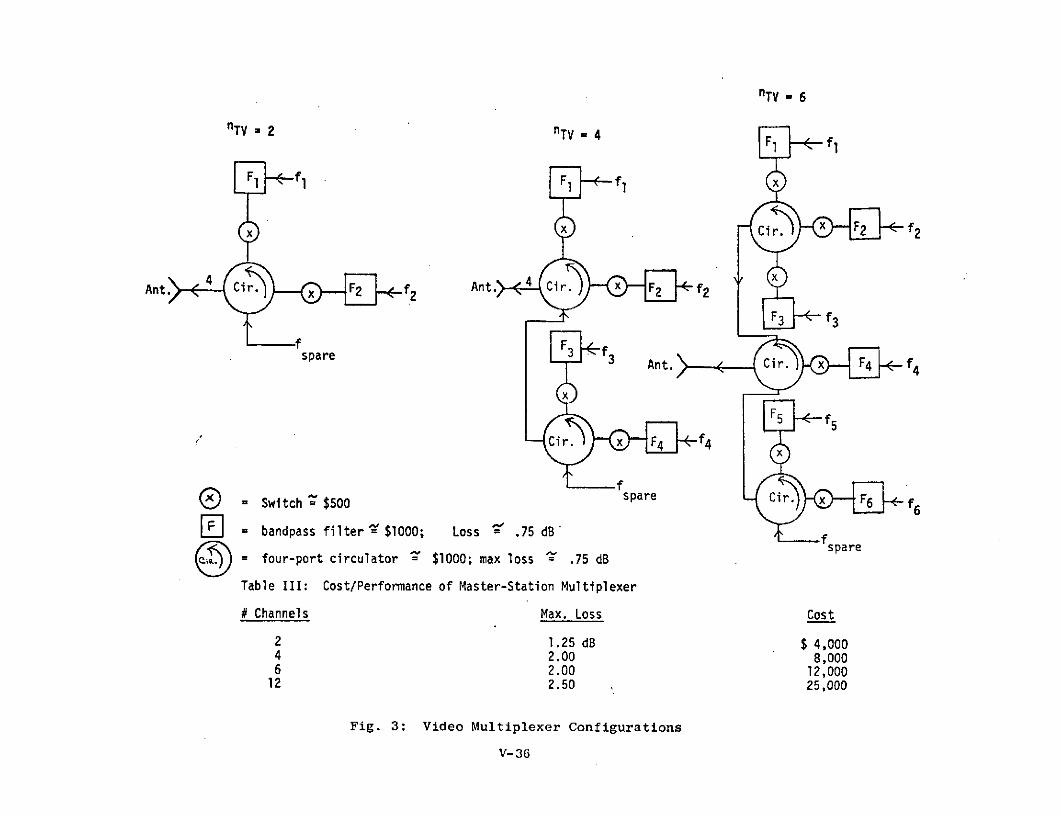
nTV * 6

nTV 2 nTV 4 f

F1 f F1 1 x

x x Ci X F2 f2

Ant. 4 Ci x F2 f2 Ant. 4 Cir x F2 f2

F3 f3

spare 3 ft3 Ant. Cir. x F4 f 4

; 4

CixF4a4 F5 Crf5

0 = Switch $500 spare F6 f

J = bandpass filter ^f $1000; Loss ' .75 dBspare

= four-port circulator = $1000; max loss ^ .75 dB

Table III: Cost/Performance of Master-Station Multiplexer

# Channels Max. Loss Cost

2 1.25 dB $ 4,0004 2.00 8,0006 2.00 12,000

12 2.50 25,000

Fig. 3: Video Multiplexer Configurations

V-36

multiplexed on a subcarrier.19 An output signal-to-noise ratio of 43 dB

or 56 dB at the 3 dB beam edge was the assumed signal-quality constraint.

Having no knowledge of available uplink frequencies, we have assumed

that both the TV and return audio would go up at 6 GHz. The downlink

frequencies have been set at 2.5 GHz and 2.2 GHz, respectively. The

ITFS band, which extends from 2500 MHz to 2690 MHz, is particularly well

suited for the distribution of educational and health materials via

satellite in view of the allocations granted at the 1971 session of the

World Administrative Radio Conference.20 Nonetheless, the number of

video channels which may be distributed in this band is limited. We have

used an RF bandwidth of 25 MHz in our calculations, implying that if more

than 7 video channels are to be distributed the band must be reused.*

For 7<n TV<15, we have assumed that orthogonal polarization would be em-

ployed; and that two pre-amps and two antennas would be used at each

slave station.

Due to the fact that the channel capacity of the ITFS band is limited,

it would appear to be attractive to multiplex several video channels

per carrier. If high-power tubes could be made available economically,

it might be more efficient to use a single transponder, having 190 MHz

of bandwidth. One could achieve multiple access in the usual way by back-

ing off from the point of saturation. Unfortunately, the present video-

baseband format leads to significant practical difficulties. The goal,

of course, is to reduce the peak-to-average factor by combining many

channels on a single carrier--the principal reason large voice trunks

are multiplexed. However, the sync pulse and the color coding at 3.54 MHz

represent distinctly non-random features, meaning that a great many video

channels must be multiplexed before the law of large numbers begins to21

take effect. And when more than three conventional video channels are

multiplexed, it is difficult to obtain the required phase linearity in a

low-cost receiver.2 2

It might be possible, however, to modify the baseband format prior

to transmitting the video signals to the satellite. It would be necessary

Threshold operation with a 3 dB space-link margin has been assumed, theobjective being to obtain an output signal-to-noise ratio of 43 dB. Cf:equation (19).

V-37

to transform the multiplexed signals into a format compatible with exis-

ting TV receivers at the receiving ground station, but the increased

equipment costs on the ground might be justified by reductions in the

space-segment charges. We recommend that this notion be pursued further.

C. Fixed Satellite Parameters: Optimization of the Ground Segment

1. Identical Slave Stations

We shall assume that one pays for the use of a TV or audio trans-

ponder on an "all or nothing" basis, the alternative being to use a ter-

restrial distribution system - or to write off the project as being econ-

omically unfeasible. A consequence of this assumption is that the para-

meters of the nimumum-cost ground stations are relatively insensitive to

the number of received video channels, nTV. Thus, once the system is

installed, the marginal cost of expanding the channel capacity is essen-

tially constant (equal to the incremental space-segment charge) until the

available bandwidth is consumed. Then one must reuse the allotted spec-

trum, increasing the ground-segment costs as well. (When both the ground

and space-segment parameters are variable, the marginal cost is a decrea-

sing function of nTV for 1 n < 7, as will be seen in Fig. 6.20 of Chap-

ter VI.

The problem of determining the minimum-cost ground-station parameters

is relatively straight-forward when the transponder parameters are fixed.

One requires knowledge of the maximum output power of the two classes of

transponder, iP sat' the input flux density in watts/feet 2 which saturates

the transponders, i x, where i = 1, 2; curves relating (C/T)im to input

backoff; the effective area of the satellite antenna, (A ) ; and thee sat

noise temperature of the receive subsystems of the transponders, TsatWe shall assume that the power transfer functions of the transponders are

linear, although the equations easily could be modified for hard limiting

or automatic-gain control.

At most 190 MHz is available in the ITFS band, which extends from 2500MHz to 2690 MHz. Assuming a 25 MHz RF bandwidth for the video signals,at most 7 channels can be distributed before the spectrum must be roused.We have assumed that two antennas and two pre-amplifiers would be usedat each slave station in this event.

V-38

The algorithm to be described is designed for rapid numerical analy-

sis. To reduce the execution time, it is helpful to decouple the analy-

sis of the slave stations from that of the master. We consider six

different pre-amplifiers and 11 transmitter alternatives in our case

studies. Thus, there are a maximum of 66 cases to be evaluated per sta-

tion. If the stations were decoupled, at most 66 + 66 = 132 cases would

need to be considered; if the parameters of the master and slave stations

were coupled, the figure would rise to 66 x 66 = 3356 cases. For this

reason, we introduce two subsidiary parameters, which are the independent

variables in the algorithm to be described.

Suppose that the video noise budget is partitioned so that (C/T) =X(C/T)

d . It follows that:

(30) (C/T) = (1 + x) (C/T) = (4n/ A v)(AP/e f)(A /T)u 1 t u TV mm m xr e sat

and that

(31) (C/T) = (1 + xl) (C/T) = [(EIRP) /BO.f ](A /T )d 1 t sat xr s swhere 1/2 the maximum

(EIRP)sat =/ effective isotropic radiated power of the satellitetransponder**

and

1, (AmPm/.mfx )>f xm m xr(32) BO=

I x/(Am P m/mf xr), otherwise.

Thus, given a value of x, the following relations may be inferred:

x must be greater than 0 to insure that (C/T)u > (C/T) . Otherwise,

the required value of (C/T) = [(T/C) - (T/C)]- 1 would be negative.

The objective is to meet the signal-quality constraint for those stations3 dB or less from beam center. If the transponder uses automatic-gaincontrol or a hard limiter, (EIRP) /BO is defined to be that fractionof the satellite output power conaining the signal. There are minor

modifications to equations (33) and (34) that are discussed in the deri-vation of equations (14) through (18).

V-39

(33) A = (1 + x) (C/T) ( \ 2u/4n) f (A /T) =(I + x)k 1mm 1 u uV m xr e sat 1

0

-1)(1 + x (C/T) f BO f (A/T)

1 t xr 1 x sat,x< " -

(EIRP)sat 1 (C/T)t

(34) A /T =s s

-1(1 + x-1 )(C/T) f (A /T)1 t x e sat

S- 1(EIRP)sat 1 (C/T)t

= (1 + x- 1 ) k4(x)

The video-link equations are the same whether TDIA or FDMA is used

to provide multiple access for the return traffic. In most cases it

proves to be cost effective to drive the TV transponder into saturation.

Even though the required uplink EIRP of the master station would be

reduced by backing off, the cost of the N slave stations would be mini-

mized by using all of the available transponder power - which one pays

for in any case.

It is essential not to saturate the return-audio transponder when

FDMA is used for the return traffic, however. As indicated in Section

B.6. it is physically impossible to meet the signal-quality constraint

unless at least 4.7 dB of input backoff is provided. (Equation (27),

on which this statement is based, was 'derived from empirical data per-

taining to Intelsat IV.) Even in the case of TDMA, for which inter-

modulation distortion is negligible, it sometimes proves to be cost

effective to conserve uplink power from the N slave stations in exchange

for increased master-station sensitivity.

Suppose that nA audio carriers must access the return-link transpon-

der. In the case of FIMA, these carriers continuously occupy the trans-

ponder in non-overlapping frequency- slots; they each receive 1/nA of the

available power. The information is modulated in bursts in the case of

TDMA, each carrier receiving the full power of the transponder in non-

overlapping time slots.

V-40

The total flux density required to saturate the audio transponder2has been defined to be f watts/feet2. Thus, for a specified input

2xbackoff, the uplink EIRP for an FDMA carrier satisfies the equation:

0

(AsPs/ )(4Tr/ 2A)/fr f /(n BO).ss s uA xr 2 x A

implying

(35) AP = ( f /n BO)x ( /4)f = k /(n BO).ss 2 x A suA xr 3 A

Given BO, (C/T). --and hence (C/T) --may be determined from equationim 2 q(27). The uplink EIRP must be sufficient to insure that (C/T)

2 f /n BO)(A/T)sat > (C/T) . Hence, BO must lie in the range:

(36) 4.7<BO (dB)<2 f + (A e/T) sat- (C/T)q - n

When nA becomes too large, a second transponder must be used.

The uplink carrier-power-to-noise-temperature ratio associated with

a particular backoff setting, BO, is simply:

(C/T) = ( f /n ABO) (A /T)sa tu 2x A e sat

To precisely meet the signal-quality constraint for the narrowband return

signal, (C/T)d must satisfy the equation:1

(37) (C/T) = 1d (T/C) - (T/C)

q u

(EIRP)sat . (A /T )

nA. BO-f xr m m

Consequently, the required master-station sensitivity in an FDMA system

is given by the equation:

V-41

BO-f 1xr

(38) A /T xr -(A_/T)(38) Am m (EIRP)sat (T/C) /nA - BO/[ 2 fx'(Ae/T)sat]

The quantity (C/T) (T/C) is bounded below by (C/T)t,2 q (T/C)t (T/C)i m

approaching the lower bound asympototically as BO and (C/T) im approach

infinity. The optimum value of BO is generally in the neighborhood of

10 dB, however; so that for FDMA 2(C/T)q = 2(C/T)t.

When TDMA is used to provide multiple access, each slave station must

transmit at the system bit rate and 2(C/T) = nA * 2(C/T) t. The equations

corresponding to (35) and (38) are:

(35') A P ( f /BO) ( u /4 )f = k'/BOss 2x suA xr 3

and

(38') A /T - xr k2(n A' BO)

(EIRP) sat (T/C) t/n - BOf (A /T)

2 x e sat

For the same backoff setting, the uplink EIRP is higher by a factor of

nA for TDMA; and the master-station sensitivity is approximately the same.

Of course, BO is not constrained to be greater than 4.7 dB in a TDMA system;

in fact the transponder is often driven into saturation, in which case

BO50 dB. As a result, the master-station sensitivity is generally less

in a TDMA system, but the slave-station EIRP is significantly higher. Con-

sequently, the cost comparisons increasingly favor FDMA as N becomes

large. This conclusion is reinforced by the fact that modem costs, which

presently are higher for TDMA systems, have not been included in the analy-

sis.

Equations (33), (34), (35) and (38) are summarized below:

Am P = (1 + x)k I

A /T = k2 (nA,BO)(39)

AsP = k3/(n BO)

-iA /T = (1 + x )k4 (x)

V-42

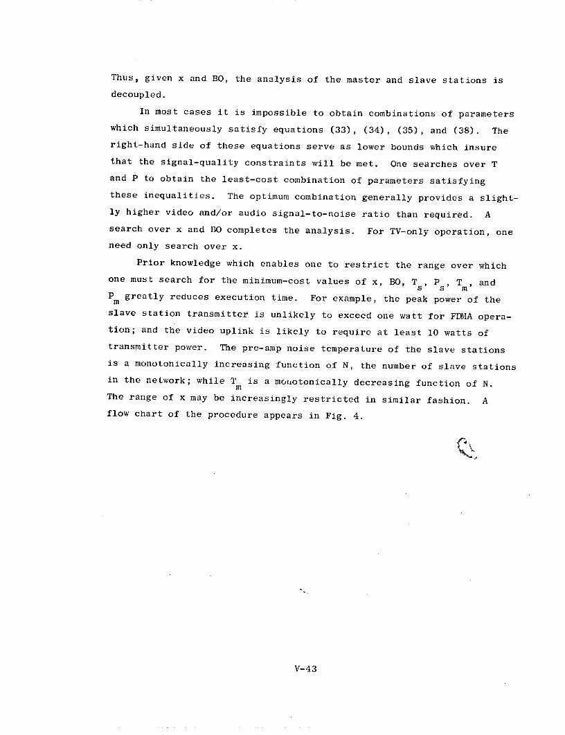
Thus, given x and BO, the analysis of the master and slave stations is

decoupled.

In most cases it is impossible to obtain combinations of parameters

which simultaneously satisfy equations (33), (34), (35), and (38). The

right-hand side of these equations serve as lower bounds which insure

that the signal-quality constraints will be met. One searches over T

and P to obtain the least-cost combination of parameters satisfying

these inequalities. The optimum combination generally provides a slight-

ly higher video and/or audio signal-to-noise ratio than required. A

search over x and BO completes the analysis. For TV-only operation, one

need only search over x.

Prior knowledge which enables one to restrict the range over which

one must search for the minimum-cost values of x, BO, Ts, Ps T m, and

P greatly reduces execution time. For example, the peak power of the

slave station transmitter is unlikely to exceed one watt for FDIA opera-

tion; and the video uplink is likely to require at least 10 watts of

transmitter power. The pre-amp noise temperature of the slave stations

is a monotonically increasing function of N, the number of slave stations

in the network; while Tm is a monotonically decreasing function of N.

The range of x may be increasingly restricted in similar fashion. A

flow chart of the procedure appears in Fig. 4.

V-43

Fig. 4: Fixed Satellite Parameters; N Identical Slave Stations

SS v = $/video transponder/year (n in all)

SSA = $/return transponder/year (nAT in all)

STARTEnter Dsat, Tsat' uTV' dXTV Set C = N106

usA ' dDA '

1(C/T) t ' 2(C/T) t' Do 6 T * T (N)SSv SSA , Ground-Segment Costs r m o

Set 4 = m sSd Sd(N)/N, T = T

Do 1N 10, 25, ..., 1,000 sSet discount factor: Do 7 P 4 P (N)

d(N) = N(.92)1og2 N . Set V + , Pm p

Ct = N106

Specify range of Set d =

x (X(N), BO B(N), T Ts(N), nTV+ 1)d(N)/N, P = ss sPs f'(N), Tm m(N)N) Set A max [c/ m , c2

a mz = Aa(A )+d Apa (T)+dpApt(P )

Compute c = (l+x)kl, If (z -GE" Cm) go to 7

c4 = (+x)k4. Cm = z, Tm m m m7 continue6 continueDo 3 B0 B(N)

Compute 2(C/T) . DeterminetSet z = C+Cm+ Sv+nATSS

Arequired number of return-lnk

nT3transponders, nAT. Set If (z GE Ct) go to 3C2 = k2(nA, BO), C3 = k3/(nAB) C t .= . =A o T =T °

p=OS SAnalysis of master and slave A' = A T = T , P= pO BOstations essentially decoupled m m m ' aat this point.

x = x

3 continue2 continue

Set Cs N6 4

Do 4 T f T (N)a sDo 5 P 4 P (N) Store the minimum-cost results forDo s s() the choice of (nTV,N,nA) under

Set As = max Tc3 /P , C4Ts consideration.Compute Aa(As) (eq'n (4)) 1 continue

z = d(N)[Aa(As)+Apa (Ts)+Apt (Ps)

If (z GE C ) go to 5

C = z, A A T = T pO Print results for N[10 1

5 continue4 continue STOP

V-44

2. Classes of Slave Stations

Suppose that there are k classes of slave stations and that

N = n(l) + n(2) + ....+ n(k). Each station is assumed to return a single,

narrowband carrier to the master station; but the video signal-quality

constraints for the various classes of stations are different. Denote

the required carrier-power-to-noise-temperature ratios by I(C/T)t ( i )

i = 1, 2, .... k. As before, the configuration of the minimum-cost

ground segment is independent of the number of received video channels,

nTV(i), i = 1, ....k, until the spectrum must be reused. The different

stations do not necessarily pay the space-segment charge required to re-

ceive all of the available channels; but we shall assume that the TV

transponders have identical performance characteristics.

Fortunately, the analysis of the k + 1 different categories of sta-

tions may be decoupled. For simplicity, we shall let k = 2. This is

a case which would arise, for example, if n(2) of the stations were lo-

cated at the point of use and n(l) of the stations were the headend of

a terrestrial redistribution system, each of which required signal-to-

noise ratio at the point of use would rest with the owners of the terres-

trial systems. We have assumed tiiat class 1 stations require a 56 dB

video signal and that class 2 stations require a 43 dB signal on the

3 dB contour.

The optimum modulation index for the video is a compromise between

that value which results in threshold operation for the 43 dB or 56 dB

stations; it edges ever close to that required by the class 1 stations

as the quantity n(l)/n(2) increases. In configuring the two classes of

stations, it is important to consider the larger discounts which accrue

when they use identical components. This situation occurs with increasing

frequency as the quantity n(l)/n(2) increases.

Suppose that the video noise budgets are partitioned so that

(1) (1)(C/T) = x .(C/T)I)

and (40) (2) (2)(C/T) = x2 (C/T)d

u -45

V-45

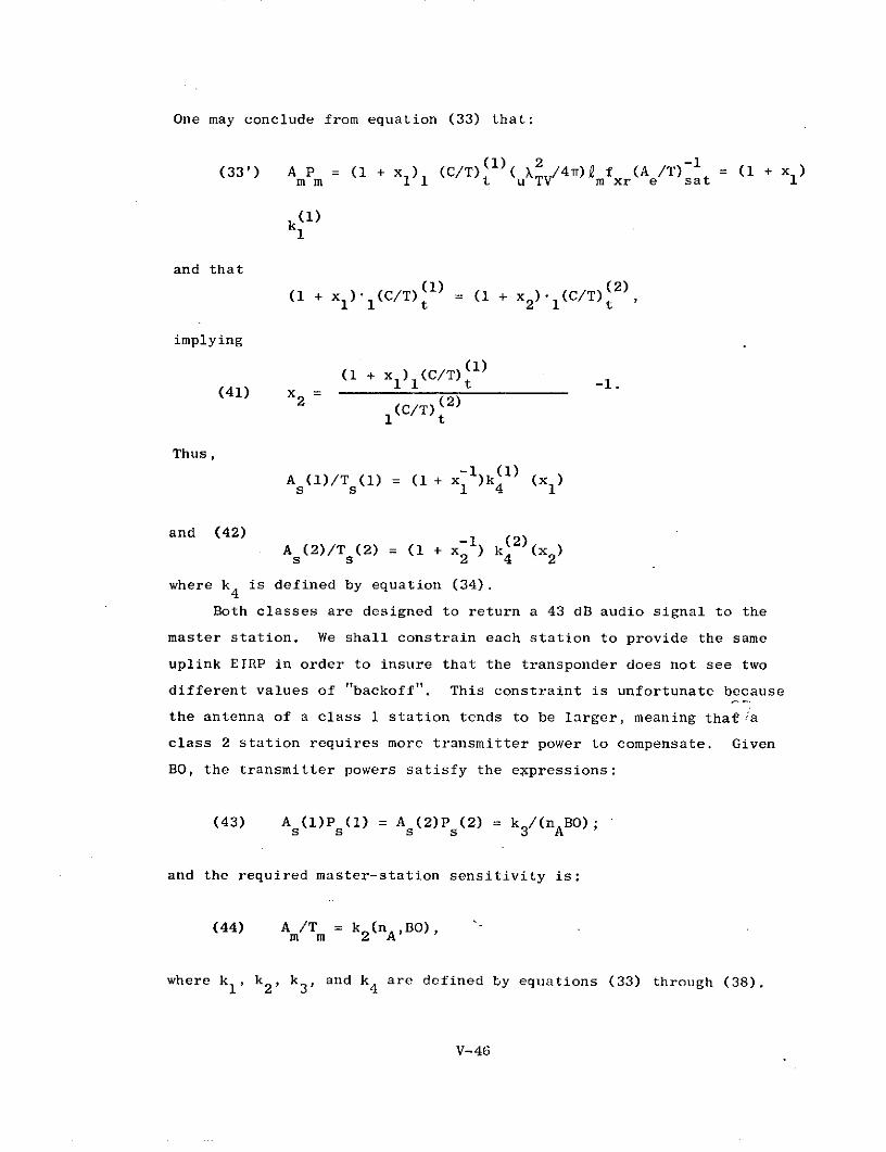
One may conclude from equation (33) that:

(33') A Pm = (1 + x ) (C/T) (1)( /4r)£ f x (A /T) -l= + x I )mm 11 t uTV m xr e sat

(1)k

and that

(1) (2)(1 + x ). (C/T) = (1 + x 2 ) (C/T)t2)

1 1 t 21 t

implying

(1 + x ) (C/T)l)(41) x =(2)

(C/T) t1 t

Thus,

-1 (1)A (1)/T (1) = (1 + x I )k4 (x I )

s s 1 4 1

and (42)As(2)/Ts(2) = (1 + x ) k ((x 2 )s s 2 4 2

where k4 is defined by equation (34).

Both classes are designed to return a 43 dB audio signal to the

master station. We shall constrain each station to provide the same

uplink EIRP in order to insure that the transponder does not see two

different values of "backoff". This constraint is unfortunate because

the antenna of a class 1 station tends to be larger, meaning that'a

class 2 station requires more transmitter power to compensate. Given

BO, the transmitter powers satisfy the expressions:

(43) A (1)P (1) = A (2)P (2) = k /(n ABO) ;

and the required master-station sensitivity is:

(44) A /T = k (n ,BO),mm 2A

where k I , k 2, k3, and k4 are defined by equations (33) through (38).

V-46

The analysis proceeds exactly as before with the exception that

there are now two discount factors to consider, corresponding to n(l)

and n(2). A single discount factor based on N = n(1l) + n(2) is used if

the stations choose to use the same pre-amplifier, transmitter, or anten-

na.

D. Optimization of Both Ground and Space Segments

1. Analysis

A primary goal of our study of teleconferencing at Stanford has

been to estimate what the cost of satellite teleconferencing could be.

To make this assessment, it is important to have the freedom to vary the

transponder parameters as well. In this section, the RF power and gain

of the video and return-link transponders are optimized to minimize the

annual cost of service as a function of the desired area of coverage,

the signal-quality constraints, the uplink and downlink frequencies, the

required channel capacity, the total number of stations, and the relative

cost of the ground and space segment.

The space segment no longer is a fixed cost. It becomes economical

to use large amounts of satellite power and a high-performance master

station only when a large number of remote stations share the cost. For

small numbers of stations, our results are substantially in agreement

with those domestic satellite filings designed to provide comparable

service, such as the Hughes/TelePrompter proposal.

Unlike the case in which the performance characteristics of the

transponders are fixed, it is possible to satisfy both the video and

return-audio signal-quality constraints exactly. We begin as before

with an arbitrary partitioning of the two noise budgets. Suppose that

(C/T) = x" (C/T) = (1 + x)1 (C/T) and (C/T)u = (C/T)d = (1 + Y)21 u 1 d 2 u 2 d(2

(C/T) q'

where

-1(2(T/C)t - (T/C) ) , FDMA

(45) (C/T) =2 q

n A'2(C/T) , TDMA

V-47

Reasoning as in the derivation of equations (33) and (34), one may con-

clude that:

Am P = (1 + x)k 1

-i (A)A /T = (1 + y ) k /Psat

(46) m m 2 sat

As P = (1 + y)k 3

A /T = (1 + x )k /P(vs s 4 sat,

where

2 -1k = (C/T) t(u TV/4) f (A /T)1 1 t uT m xr e sat2 -1k = (C/T) ( 2 /4Tr)f (A )12 2 q dA xr e sat

k = (C/T) q(u 2/4Tr) f (A /T ) s3 2 q uA s xr e sat2 -lk = (C/T) ( 2 TV/4r)f (A )-4 1 td TV xr e sat

(A)Psat = RF satellite power per video channel

t"Useful" RF satellite power per audio chan-(A) ni*, FDMAsat= Total RF satellite power for the return

traffic, TDMA

To determine (C/T)im, which is needed to compute 2 (C/T)q in the case of

FMIA, the input backoff must be specified. Unlike the fixed transponder

case, y and BO may be varied independently. The range over which one

must search for the optimum value of BO is modest, as indicated in sec-

tion B.6.; but unfortunately there is no way of determining the appro-priate range of x and y a priori. We determined the optimum values

through a method of trial and error. x and y were allowed to range overa span of 10 dB in increments of one dB. If the minimum did not occurat an interior point, the range was appropriately modified. A plot ofthe optimum values of x and y for one of the cases analyzed appears inFig. 6.15.

The "useful" satellite power is defined to be the required satellitepower per channel divided by the input backoff, BO. The space-segmentcharges are proportional to BO.p(A)

sat

V-48

Having specified x, y, and BO, the analysis of the ground-segment

parameters for the master and slave stations is decoupled. Referring to

equation (4), the objective is to minimize the expressions:

(48) C (x,y,BO) = k(N,n ) [a (i) + a (i)A a3(i)+ A (T )] + d(N)s TV 1 2 s pa s

-1A (P ) n TVSS-(1 + x- )kT /Aspt s TV 4s s

and

(49) C (x,y,BO) = a (j) + a (j)A a3 (i)+ A (T ) + d(n TV+1)Aptm 1 2 m pam TV pt

(P ) + C mp(n TV) + SS.*( + y )'k 2 * A B

1, TDMA

subject to:

(50) APs (1 + y)k 3

A P (l + x)k 1

where Cmp(nTV) is the annual cost of the multiplexer required at the

master station to combine the nTV video carriers; and

N.(51) k(Nn(.92) g2 N , 1 nTV <7

2N'(. 9 2 )log2(2 N) 8<n TV 14;

(52) d(N) = N-(.92) log2 N

i, j 1,2,3 . T ETs(N); Ps E P s ( N); Tm T (N), and P m P (N).

Consider the problem of minimizing C s(x,y,BO). For the moment,

neglect the influence of P and inequality. (50a). Then for fixed i ands

T s, the optimum value of As may be obtained by differentiating equation

(48), giving rise to the expression:

(53) As(x,Ts,i) = nTV*SS(l + x -1)k4T/[k(N,nTV)a2(i )a3(i)]/[a (i)+]

where i=l, 2, 3. Initially, one sets i=l, assuming implicitly that

V-49

D [A (x,T ,1)]412'. Should this assumption prove to be incorrect, one

may conclude that D [A s(x,T,1) ] = 12', a consequence of the fact that

C is a convex function of A for fixed i; Ts , and P . If the solution

lies on the boundary, one evaluates equation (53) for i=2. For this

case, the extremal value is constrained to lie in the interval 12'

Ds [As(x,Ts,2)] 40'. (Cf: equation (4).) Should the solution lie on the

outer boundary, one must evaluate (51) for i=3. One selects that value

of i which minimizes (48) for fixed T and P , Denote this quantity by:s s

(54) As(x,T ) = min A (x,T ,i)i=1,2,3

In view of inequality (50a), the optimum value of A for fixed Ts s

and P satisfies the equation:s

(55) AO(x,y,BO,T ,P )= max (1 + y)k3/P, A (x,T ) .Ss 3 s

Finally, one searches over T s T (N) and P E P (N) to obtain the global

minimum of C (x,y,BO). Denote the associated parameters by To and Po.s s s

C m(x,y,BO) is minimized in similar fashion, giving rise to the0

parameters Am, Tm, and Pm. In general, (50a) and/or (50b) are strict

inequalities at this juncture. Consequently, P () and/or P A) may besat sat

slightly reduced from the values given by equations (46b) and (46d),

which were based on the assumption that (50a) and (50b) would be exactly

satisfied. Reasoning directly from the definition of the noise budgets,

as given by equation (2), it may be shown that:

C is convex in A for fixed T , P , and i if the antenna cost rises at

least as rapidly as the effective area. Indeed, if this were not thecase, the cost data would be suspect.

V-50

k (A /T-

(56) P (x,y,BO)=sat k

1

Ao pOm m

(57)

k (Ao/To) - 1

(A) 2 m mP (x,y,BO) =sat k

1 - o pOs s

where kl, k2 , k3, and k4 are defined by equations (47). The annual cost

of the system, for the particular triplet (x,y,BO) under consideration,

is given by the expression:

(57) Ct(x,y,BO)=k(NnTV) [A (A ) + A (To)]+ d(N)A (Po) +.t TV a s pa s. pt S

A (Ao) + A (TO) + d(n + 1) A (Po) + SS n Pv)a m pa m TV pt m TV sat

nnABO, FDMA Cmp(nTV)'

1, TDMA mp TV

A search over x, y, and BO completes the analysis. The required power

gain of the video and return-audio transponders is computed in the last

step.

It is essential to incorporate any prior knowledge that is available

to restrict the range of alternatives in x, y, BO, T , Ps' , Tm , and Ps s m m

that must be considered. The alternatives may be increasingly refined

as the optimum is approached. A flow chart of the algorithm that we have

developed to estimate the cost of a satellite teleconferencing system when

both the ground and space segment are variable appears in Fig. 5.

2. Summary of Results

We have analyzed a total of 48 different problems in an effort

to gain quantitative knowledge of the impact on the annual cost of cer-

tain system parameters known to the decision maker a priori. D a wassat

V-51

STARTT-Ent sat Tsat' uTV' Set C = N10

6

d u A d , (C/T), md TV' u A' d A 1(C/T) Do 8 Tm T (N)

2(C/T)t , SS, Ground- Compute A- (y,BO,T )

Segment Cost Data, T

Set dTd(N)/N, T = To

m sDo 1

nTV - f2,4,6,12) Do 9 P P (N)m m

Do 2 N - 10, ..., 10,0003 Compute A'(x,y,BO,Tm,P )Set d(N), K(N,nTV), Ct = N10 Compute Aa(Am), u = SSc2 Tm/Am

Specify range of x - X(N), y - (N) n +1, P PBO B(N), T *T (N), P P (N), Set TVl m

s s Set dp (nTV+)d(N)/N P =T T (N), P P (N) V ' m sTm m m

z = Aa(Am)+dApa (T m + dpApt(P m)+u

If (z *GE" C ) go to 9Do 3 x - X(N) C = z, A , T P0

= PCompute c = (1+x)k I m= z, A =

A'm m m

c 4 = (1 + x )k 4 Cm C - u9 continue8 continue

Do 4 BO B{N)Compute 2(C/T)q (v) (A)

Do 5 y (N) sat sat Set

Compute c3 (1 + y)k 3 = C +C + SSn (A) ABO F DM Ay m sa'

nA-BO, FDMA TDMAc 2 = ( + y )k2 If (z *GE- Ct) go to 5

1, TD MACt = z, A = A, T =o, p0 ' s T0 s s

6 Am-=Am Tm m mm, m = BO,Set C = N10 6 = m m m ms = b 6 (v) = (V), -(A) (A)

Do 6 T T (N) sat sat' sat sats s 5 continueCompute A'(x,T ) 4 continue

Do 7 P - P (N) 3 continues s

Compute A s (x,y,BO,T s ,P )

Compute Aa(As) , u = SSc4Ts/A' Store minimum-cost results for par-SA ( u ticular choice of (N,nTVnA) Underz = k(N,nTV ) A a(A) + Apa (Ts ) + consideration.

d(N)Apt (Ps ) + u 2 continue1 continue

If (z "GE- C ) go to '7sS= Ts =

-As As Print results for N = 0, ..., 10,000;

Cs = Cs - u TV= 2,4,6,12

7 continue6 continue

Fig. 5: Variable Satellite Parameters

N Identical Slave Stations

V-52

set at 6' or 10', values which correspond to continental U.S. coverage

or regional coverage at 2.5 GHz; SS, the annual cost per watt of RF

satellite power, assumed values of $15,000, $30,000, or $50,000 -; voice

or digital feedback was assumed; and either FDMA or TDMA was used to

provide multiple access to the return-link transponder, the uplink fre-

quencies for the video and return traffic were assumed to be 6.0 and 2.25

GHz respectively. The stations were assumed to be located at the point

of use, and a 43 dB video signal for those stations located along the 3 dB

beam edge was the assumed signal-quality constraint. For each case, 2,

4, 6, or 12 video signals were to be received by each of the N slave sta-

tions. N was allowed to assume values of 10, 25, 50, 100, 250, 500, 1000,.

2500, 500, or 10,000.

The voice-feedback systems were configured for continuing profession-

al education. Having no knowledge of return-traffic statistics, we made

some arbitrary assumptions. A minimum of one return channel per video

channel was allocated on the satellite. Additionally, one channel was

allocated per 50 remote classrooms.

Class size would be extremely limited if all questions were rebroad-

cast. Consequently, we have assumed that multiple voice channels would

accompany the video. Additional personnel would assist the instructor

at the video-origination center by fielding questions from remote stu-

dents and informing the instructor of their general drift. As many of

the return channels as possible would be designed for duplex operation.

One of the forward channels would transmit data, intended in part

to indicate which of the return channels were presently available. There

is no provision for avoiding multiple seizure of these vacant channels,

however. Sufficient return channels must be available to reduce the prob-

ability of such occurences to an acceptable level.

In the case of digital feedback, each station was assumed to contin-

uously access the satellite with a single audio carrier. Thus, nA = N.

As will be seen (cf: Fig. 6.21), the cost of return-link power is dwarfed

by the remaining components of the annual cost. This scheme, which easily

could be implemented, is only 5% to 25% more expensive than the voice-

feedback procedure discussed previously.

Some of the significant results of these case studies appear in

Fig. 6. Figures 6.1 through 6.16 compare FDMA with TDMIA. For each of

V-53

Audio F.B., SS = $30K, D = 10'sat

FDMA TDMA

1. Cap. Cost (S) ($K) 2. Cap. Cost (S) ($K)

64 12 64 1212

16 k\ 16

4 2 42

I I

-25 -25

to IO' 104 10 10 I03 104

3. Cap. Cost (M) ($K) 4. Cap. Cost (M) ($K)1000 500 nTV =12

500 250 6

250 12 125

125 6 62.5

62.5 2 31.25

1o 16 106 10, 10 102 10 10

5. ANN Cost/N ($K) 6. AANN Cost (%)64 70

16 55 nTV= 4

4 40

I 1 25

-25 10

10 102 10 10 10 102 o10 104

Figure 6: Variable Satellite Parameters

V-54

Audio F.B., SS = $30K, Dsa t = 10

FDMA TDMA

7. Sat. Cost ($K) 8. Sat. Cost ($K)12

2000 2000

61000 4 1000 6

500 2 500 4

250 250 2

125 125

10 10 103 104 10 102 103 104

9. Diam. (S) (ft.) 10. Diam. (S) (ft.)

12 19 12

17 17

15 15 4 6

13 13

II II 2

10 102 I0 I 10 102 IO3 104

11. Diam. (M) (ft.) 12 12. Diam. (M) (ft.)40- 6 40

432- 2 32 12

/624 24

16 16 42

8 8

10 102 103 10 10 t 0 104

Figure 6: FDMA vs. TDMA (cont.)

V-55

FDMA TDMA

(v) (A)13. P (Watts) 14. P (Watts)

sat sat

10 3.2 48

FDMA

8 1.6 24TDMA

6 0.8 12FDMA

4 0.4 06

2 0.2 03

12

10 Io? IO3 lO* 10 102 10 10I

15. Noise Budgets (dB) 16. Noise Budgets (dB)

25 30

20 X 24 X

15 nTV 4 18 ,TV= 4

10 12

y5 6 y

10 o102 10 10 10 10o 10 I04

17. ANN Cost/(N + nTV) ($K) 18. First Lost/N (= 1/%r(N)

9 1.0

3 0.8

I 0.6FDMA ONLY Normalized First

33 - . 0.4 Cost N

.11 4 0.2 p N 1/ N

26

10 102 103 10 10 102 1I0 10'

Figure 6.13 - 6.16: FDMA vs. TDMA (cont.)

V-56

these figures, Dsa t = 10', SS = $30,000, and nA = nTV • [1 + (N + 25)/50].

The capital cost of the slave stations is displayed in Figs. 6.1 and 6.2;

and the capital cost of the master stations appears in Figs. 6.3 and 6.4.

The total space-segment charges are plotted in Figs. 6.7 and 6.8. The

slave stations are much less expensive, the master station is much more

expensive, and the space-segment charges are slightly higher in an FX.A

system. Consequently, the cost comparisons favor FDMA for large values

of N. This point is made explicitly in Fig. 6.6, which displays on a

percentage basis the relative cost of the two systems. Note that for

small values of N, TDMA is slightly less expensive--assuming that the mo-

dem costs are comparable. The basis for these relative costs is explain-

ed in equations (35) through (38') of Section C.l: The slave-station

EIRP may be reduced in exchange for increased satellite power and master-

station sensitivity when FDMA is used. Note that the capital cost of a

TDMA station actually increases for large values of N, despite the reduc-

tion in the per-unit cost of the components. The cost of providing the

necessary EIRP begins to dominate.

The annual cost per slave station is plotted in Fig. 6.5; and the

annual cost per station per video channel appears in Fig. 6.17. It

would appear that the annual cost of a satellite teleconferencing net-

work could be quite modest. By contrast, the cost of leasing common-

carrier facilities to distribute a single video channel is approximately

$30 per mile per month.20 Thus, if there were at least 25 stations in

the network, a satellite distribution system would be cost effective if

the average internodal distance were at least 10 miles. Note that the

cost drops sharply as N increases and that these cost-estimates include

provision for return audio. We would anticipate a decline in the rate

structure of common-carrier facilities when competition from dedicated

satellite networks begins to materialize.

The slave station and master station antenna diameter for a TDMA or

an FDMA system is plotted in Figs. 6.9-6.12. Note that the slave stations

would be sufficiently compact to locate on a small building and that the

diameter of the master-station antenna never exceeds 40'. Small-antenna

systems do appear to be cost effective.

V-57

The required RF satellite power per video channel is plotted in

Fig. 6.13. These modest powers per 25 MHz transponder are available

with state-of-the-art technology. For example, the Hughes HS-336 is

being designed to provide a total of 100 watts of RF power under a

weight constraint that would permit insertion with a Thor-Delta launch

vehicle.

The required RF power for the return-audio transponder is plotted

in Fig. 7.14 for TDMA and FDMA with nTV = 4. The minimum-cost TDMA

system requires significantly less satellite power; for the networks un-

der consideration, the space-segment cost for the return audio is but

a small fraction of the total cost.

Note from Figs. 6.9-6.14 that the parameters of the minimum-cost

system are sensitive to changes in N and nTV. (They are also sensitive,

but to a lesser extent, to changes in NA.) The minimum-cost values of

T s, P s , T , P , and BO, which are not as volatile as the antenna diameters

and transponder powers, have not been plotted. Neither the traffic sta-

tistics or the total demand for slave stations are likely to be known

with precision. Rather than attempt to minimize the annual cost of the

network, the supplier probably would seek a configuration which would

provide a satisfactory return on investment in the face of extreme, but

not improbable, fluctuations in demand.

x and y, the subsidiary variables which partition the video and

return-audio noise budgets in the optimization procedure, appear in

Figs. 6.15 and 6.16. For the asymmetrical links under consideration,

the uplink noise in the video link is usually much more than 10 dB above

the downlink noise, a figure which is sometimes assumed to be optimum.

There are significant economies of scale in an asymmetrical satellite

teleconferencing network. A normalized value of the "first cost" of the

network on a per-station basis is plotted against 1/N in Fig. 6.18.. The

curves are virtually indistinguishable. That is, the capital cost of the

network rises approximately as %N.

The percent increase in the annual cost incurred by adding a return

capability to the minimum-cost, TV-only network is plotted in Fig. 6.19.

The figure ranges from 8% to 28% becoming increasingly large as N increa-

ses. When there are less than 1000 stations in the network, the increase

is less than 20%.V-58

Audio F.B., SS = $30K, D = 10', n = 4 - unless otherwisesat TV

specified

19. A ANN Cost (2-way) (%) 20. Marg. Cost of Video Channel

30 $100,000

15 100

10 10

10 10 I' 10 0 3 6 9 NTV

21. A ANN Cost (D.F.) (%) 22. Cap. Cost (S) vs. ANN Cost.

35 20

Cap. Cos1

28 2

221 2

14 2

7 2

10 10 103 104 1.0 3.0 5.0 ANN Cost.

23. ANN Cost. /N ($K) 24. ANN Cost. /N ($K)

27 27

9 9

3 3

Ds= I.33 SS = 30K1 s '

50K

10 I06 103 10 10 16 10 10

Figure 6: Misc. Cost Comparisons (FDMA)

V-59

E. Symmetrical Satellite Teleconferencing Networks

We have restricted our attention thus far to networks in which there

is a one-way wideband capability and a narrowband-return capability. We

shall now consider three network configurations having greater symmetry:

1. Two-way video (or two-way audio with no video). N identical

stations.

2. One-way video with symmetrical two-way audio. The N

identical slave stations may now communicate with each

other as well as with the video-origination center.

3. One-way video plus two-way audio in a network for which

the various stations have vastly different voice-circuit

capacity requirements. (For example, the ground stations

may also be intended to serve as distribution centers for

a long-haul telephony network.)

Once again, the traffic requirements are assumed to be known. The

objective is to determine the parameters of that satellite communication

network which provides the desired grade of service in such a way as to

minimize the annual cost. Single-channel-per-carrier-per-transponder

video is assumed and FM/FDMA is used to modulate the audio information.

Two classes of transponder are available, one of which is optimized to

carry video traffic and the other to carry the voice (or data) traffic.

The transponders are modeled as linear repeaters.

We have obtained quantitative results for question 1, and the formu-

lation of question 2 is complete. The results for question 3 are quali-

tative, and will remain so until further cost information becomes avail-

able.

1. Two-Way Video

Suppose that all N stations in the network are to receive

and transmit nTV video channels. Assume also that the signal-quality

constraint is the same for each station. Letting (C/T)t be the required

carrier-power-to-noise-temperature ratio for each link and assuming that

the noise budget is partitioned so the (C/T)u = x(C/T) one may conclude

from equation (2) that:

(C/T) = (1 + x) (C/T)u t

and-1

(C/T) d = (1 + x ) (C/T) t

V-60

The preceding equations may be expressed in terms of the system parame-

ters, giving rise to the following relations:

-1 2 (v)(58) A /T = (1 + x ) (C/T) f ( /4Tr)/[(A ) P ] = (1 +s s t xr d TV e sat sat-1 (v)

x )/Psat

(59) AP = (1 + x) (C/T) f (X /4r)(Ae/T) -l = (1 + x)k .ss t xr s u T e sat 1

Suppose that there is one spare uplink transmitter at each station. Then

a total of N(nTV + 1) transmitters will be needed in all. The annual

cost of the network may be approximated by the expression:

(60) Ct = d[N(nTV + 1)] A pt(P ) + k(N, n TV)[Aa (A ) + A pa(T )]

-1+ SSnTV* (1 + x )k T /A + C (n TV).TV 2s s mp TV

where d(') and k(.,.) are defined by equations (51) and .(52).

For each value of x, Ct may be minimized in the manner outlined in

equations (48) through (55). One then searches over a range of x (which

through previous experience contains the optimum for the particular set-

tings of SS, N, and nTV under consideration) to obtain the global minimum(v)of C . In the process, the optimum values of As, Ts, Ps, sat and the

power-gain of the transponder are determined.

Numerical results have been obtained for a network consisting of N

two-way video stations, for N- 2, 4, 8, 16, 32, and 64. nTV assumed

values of 2, 4, 6, and 12; SS was set at $30,000/watt/year; and D atsat10'. The output signal-to-noise ratio was constrained to be at least

43 dB within the 3 dB cone of coverage.

The annual cost per station is plotted in Fig. 7.1. While much

higher than before, it is intriguing. If expensive new communications

services become a substitute for transportation, two-way video may be

among the first to be successfully marketed. Large cities could be

equipped with studios in which individuals could participate in small

tele-conferences. The cost of periodic board meetings or sales meetings

V-61

SS = $30K, -D = 10'sat

1. Cap. Cost (S) ($K) 2. ANN Cost/N ($K)

400 160

200 80

12 12

50 20

6 6

25 4 10 42 2

4 16 64 4 16 64

3. Diam. (ft.) 4. Psat(v)Watts)

29 4.82

26 2-4 4

6

23 1.2 12

20 12 0.6

-617 0.3

-- ~ -- ~- - 24 16 642 4 16 64

Figure 7: Two-Way T.V.

V-62

could be significantly reduced--if the substitute proves to be acceptable.

The capital cost of the ground stations is plotted in Fig. 7.2.

Again, the figures provide a preliminary indication of economic feasibi-

lity.

Finally, the antenna diameter of the minimum-cost stations and the

required RF power per satellite transponder for transmission in the ITFS

band appears in Figs. 7.3 and 7.4. For this symmetrical network, con-

siderably more of the cost burden is placed on the ground.

2. One-Way Video Plus Symmetrical Voice

Suppose now that the network is designed for one-way video

plus symmetrical voice. Support that the video noise budget is parti-

tioned so that (C/T) = x*(C/T)d and that the audio noise budget is par-

titioned so that (C/T) = y'(C/T) . Letting (C/T)t and (C/T) be the

signal-quality constraints for the video and audio links, respectively,

the sensitivity of each station must be such that:

(61) A /T 2 max (1 + x-) 1 (C/T) f xr(dX 4)/[(A ) P (v)s s txr d T esat sat

2 (A)(1 + y 2 (C/T) f ( X. /4n)/[(A ) P (A)2 q xr d A e sat sat

(A) (v)where P sat and P sat(v) is the "useful" RF satellite power allocated per

sat sataudio channel and per video channel, respectively. If the signal-quality

constraints are exactly satisfied, as will be the case in the minimum-

cost network when both the ground and space-segment parameters are vari-

able, one may conclude that:

( + y -l) (C/T)( X /4r) (1 + y)k(A) 2 q d A (v) 5 (v).sat (1 + x-1 )(C/T)t(d 4r) sat (1 + x - ) sat

Thus, the annual cost of the network is approximately:

V-63

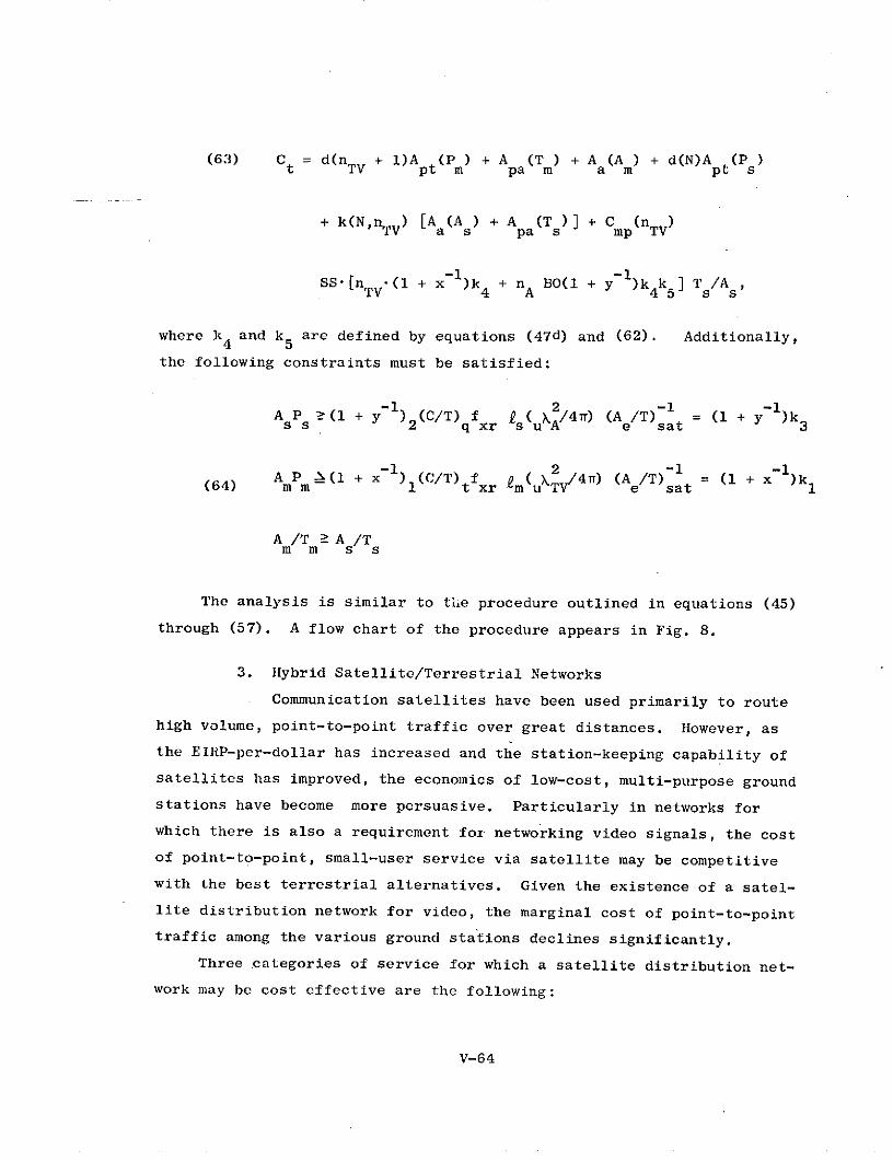
(63) C =d(nTV + 1)A pt(P ) + A (T ) + A (A ) + d(N)A (P )t TV pt m pa m a m pt s

+ k(N,nTV) [A (As ) + A pa(T )] + C mp(n TV)

SS'[n *(1 + x- )k4 + nA BO(1 + y- )k k ] T s/A s ,

where k 4 and k 5 are defined by equations (47d) and (62). Additionally,

the following constraints must be satisfied:

-) 2 -1 -l~k 3AP -(1 +y ) (C/T) f s ( u /4r) (A /T) t (1 +ss 2 q xr suA e sa 3-1 2 =

AP (1 + x- ) (C/T)tf xr (u /4) (A /T) = (1 + x )k(64) mm 1 t xr T e sat

A /T A /Tm m s s

The analysis is similar to the procedure outlined in equations (45)

through (57). A flow chart of the procedure appears in Fig. 8.

3. Hybrid Satellite/Terrestrial Networks

Communication satellites have been used primarily to route

high volume, point-to-point traffic over great distances. However, as

the EIRP-per-dollar has increased and the station-keeping capability of

satellites has improved, the economics of low-cost, multi-purpose ground

stations have become more persuasive. Particularly in networks for

which there is also a requirement for networking video signals, the cost

of point-to-point, small-user service via satellite may be competitive

with the best terrestrial alternatives. Given the existence of a satel-

lite distribution network for video, the marginal cost of point-to-point

traffic among the various ground stations declines significantly.

Three categories of service for which a satellite distribution net-

work may be cost effective are the following:

V-64

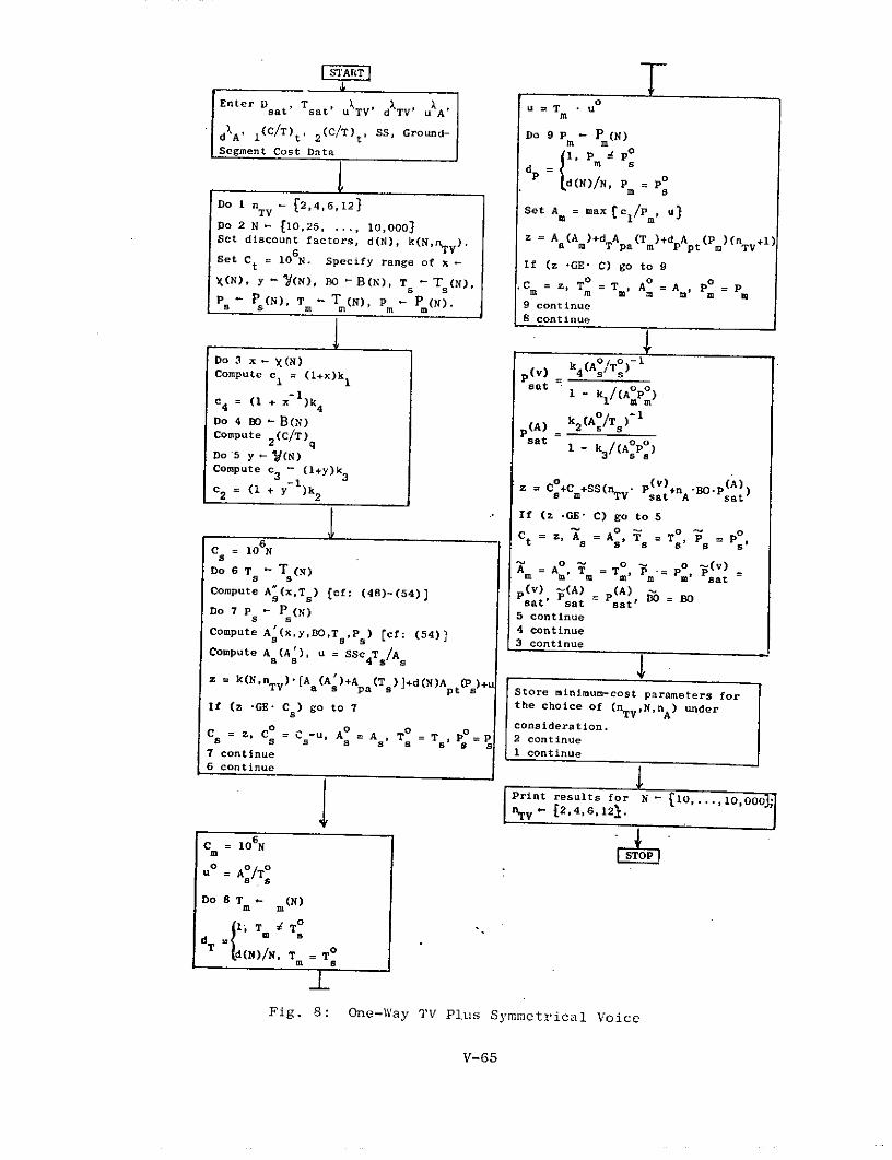
L ̂ -_J -Enter D ,T , X , u = T usat Tsat' u TV' d TV' u A u = Tm

dA ' I(C/T) t 2(C/T) t, SS, Ground- Do 9P - P (N)

Segment Cost Data 1, P m Po

dP= m sd(N)/N, P = P

m sDo I nTV -2,4,6,123

Set Am = max Ccl/Pm, u}Do 2 N- E10,25, ... , 10,000Set discount factors, d(N), k(N,nTV). = AAm)+d a pa )+d A P pt m)(n T

Set C t = 10 N. Specify range of x - If (z *GE* C) go to 9

X(N), y (N), BO - B(N), Ts T (N), Cm = z, Tm = T, A = Am' PP P (N), Tm - T(N), Pm P(N). 9 continue

8 continue

Do 3 x - (N) k (Ao/T -Compute c = (1+x)k p() 4 s s

1 1sat

c4 = (1 + x )k4 I - k/(Am

Do 4 Bo - B(N) (A) k2(Ao/Ts - 1Compute 2 (C/T)q Psat 1 - /(Apo)

Do 5 y - (N) 3Compute c3 - (1+y)k 3

C + ")S P(V)+n "BO (A)c2 =( + y )k2 = CCm+SS(nTV sat A OPsat

If (z .GE" C) go to 5

Ct = z,A A o = ToP =PC = 106 s

Do 6 T T (N) A= Ao = T o sat(v)s s m m m P m sat

Compute A (x,Ts) (cf: (48)-(54)] p , (A) = (A) BOsat sat sat'Do 7 P - P(N) 5 continue

Compute A (x,y,BO,T ,P ) [cf: (54)] 4 continues as 3 continue

Compute A (A'), u = SSc4Ts/As

z = k(NnTV)*[A (A')+A (T )J+d(N)A t)+uk(NnTV (A+As pa (Tpt)+ Store minimum-cost parameters for

If (z -GE- Cs ) go to 7 the choice of (nTV,N,nA) under

z, C C-U, A A T consideration.C s = s A = A T T Pos=P 2 continue

7 continue 1 continue6 continue

Print results for N 10, 000l nTV [ f2,4,6,121.

C = 106 N STOP

uo =Ao oB s

Do 8 T - (N)a m

=1, T d To

dT =t m sdT (N)/N, T = T

m a

Fig. 8: One-Way TV Plus Symmetrical Voice

V-65

1. Multi-purpose service to remote users in regions where thepopulation density is low;

2. Predictable point-to-point service (which periodically couldbe re-routed according to a predetermined schedule) for whichthe cost of terrestrial facilities, due to the inordinateamount of required switching, may be relatively high. Candi-dates for services include numerous business functions, suchas inventory control, check clearing, and the general problemof periodically transferring data from one memory bank toanother.

3. Switched point-to-point service in conjunction with existingterrestrial facilities. Satellites could provide a convenient"toe in the water", useful in assessing traffic patterns priorto investing in high capacity terrestrial links.

We shall discuss some preliminary findings regarding how a communication

satellite could be used to complement existing terrestrial facilities.

These results are rudimentary because we lack information concerning

switching costs, which vitally affect the cost of point-to-point service.

Some observers estimate that the cost of switching represents approxi-

mately 75%-85% of the cost of AT&T in establishing a typical long-dis-

tance phone circuit.1 7

Qualitative descriptions of switching costs are available from Bell

System publications--although quantitative information is conspicuously

absent. A "switching machine" performs two basic functions: it routes

all calls which enter the network to the intended destination and con-

centrates the traffic so that calls are not carried on small, ineffi-

cient circuit groups. The switching mechanism also performs those an-

cilliary functions essential to any complex communications network, such

as translation, signaling, and billing.

Weber 2 3 discusses quite succinctly the implications of switching

costs on the configuration of a terrestrial network. There are two basic

structures, the star and the mesh, which are depicted schematically in

Fig. 9. In a mesh network, all traffic between a pair of nodes is

carried over a single trunk (when nb alternate routing is allowed). In

a star network, the majority of calls are switched at a central node.

No intermediate switching is required in a mesh network; but due to the

lighter loading of the individual links, the trunks of a mesh network

V-66

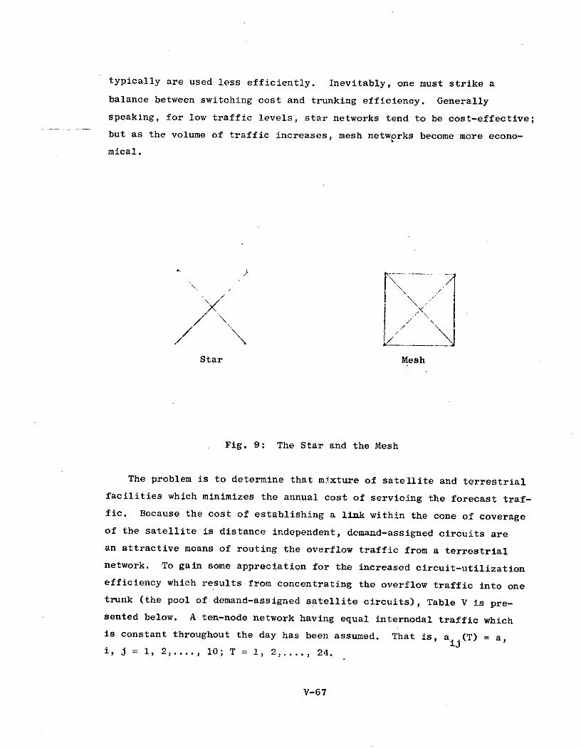
typically are used less efficiently. Inevitably, one must strike a

balance between switching cost and trunking efficiency. Generally

speaking, for low traffic levels, star networks tend to be cost-effective;

but as the volume of traffic increases, mesh netwprks become more econo-

mical.

/ \N

Star Mesh

Fig. 9: The Star and the Mesh

The problem is to determine that mixture of satellite and terrestrial

facilities which minimizes the annual cost of servicing the forecast traf-

fic. Because the cost of establishing a link within the cone of coverage

of the satellite is distance independent, demand-assigned circuits are

an attractive means of routing the overflow traffic from a terrestrial

network. To gain some appreciation for the increased circuit-utilization

efficiency which results from concentrating the overflow traffic into one

trunk (the pool of demand-assigned satellite circuits), Table V is pre-

sented below. A ten-node network having equal internodal traffic which

is constant throughout the day has been assumed. That is, aij(T) = a,

i, j = 1, 2,...., 10; T = i, 2,...., 24.

V-67

We shall dimension the system to have an overall loss of 3%. The

demand-assigend traffic will suffer a multiple loss arising from three

potential bottlenecks in the journey: existing from the origin station

(all of the available modulators may be occupied), gaining a demand-as-

signment circuit on the satellite, and entering the destination station

(where, again, the available demodulators may be occupied). To determine

the best partitioning of the allowed 3% loss, one must perform an econo-

mic tradeoff between the cost of modulators and uplink transmitters,

voice channels on the satellite, and the cost of demodulators. We do

not have sufficient cost data to perform this tradeoff at the present

time. Quite arbitrarily, we shall permit a 2% loss on the satellite and

a .5% loss at each end. The terrestrial trunks are configured for a

3% loss.

A total of 180 terrestrial trunks are required to provide the neces-

sary interconnections, assuming a mesh configuration is used. A 100%

increase in voice traffic is forecast, which may be serviced either by

increasing the size of the terrestrial trunks or by routing the overflow

traffic to the satellite. Displayed are the number of simplex circuits

per trunk required to route the present load; the increase in the capa-

city of each trunk required to route the forecast load; the total requir-

ed increase (180 timesAM..); the number of satellite circuits required13

to carry the forecast overflow traffic* ; and the ratio of the total re-

quired increase in terrestrial circuits to the number of satellite cir-

cuits.

* 24We used Wilkinson's methods to make this calculation. Given the meanand variance of the overflow traffic from the terrestrial trunks, onemay compute the "equivalent random traffic" having the same mean andvariance as that of the graded multiple. It is then a simple matter tocompute the number of satellite circuits required to service the over-flow traffic from the graded multiple at a loss less than or equal to2%.

V-68

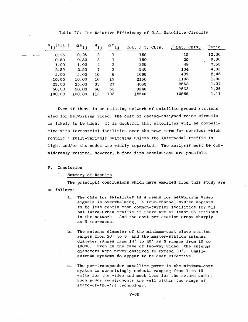
Table IV: The Relative Efficiency of D.A. Satellite Circuits

a (crl.) a* M. MRaij ij ij ij Tot. T. Ckts. / Sat. Ckts. Ratio

0.25 0.25 2 1 180 15 12.00

0.50 0.50 3 1 180 20 9.00

1.00 1.00 4 2 360 48 7.50

2.50 2.50 7 3 540 134 4.035.00 5.00 10 6 1080 435 2.48

10.00 10.00 16 12 2160 1138 1.9025.00 25.00 33 27 4860 3553 1.3750.00 50.00 60 53 9540 7563 1.26

100.00 100.00 113 103 18540 16686 1.11

Even if there is an existing network of satellite ground stations

used for networking video, the cost of demand-assigned voice circuits

is likely to be high. It is doubtful that satellites will be competi-

tive with terrestrial facilities over the near term for services which

require a fully-variable switching unless the internodal traffic is

light and/or the nodes are widely separated. The analysis must be con-

siderably refined, however, before firm conclusions are possible.

F. Conclusion

1. Summary of Results

The principal conclusions which have emerged from this study are

as follows:

a. The case for satellites as a means for networking videosignals is overwhelming. A four-channel system appearsto be less costly than common-carrier facilities for allbut intra-urban traffic if there are at least 25 stationsin the network. And the cost per station drops sharplyas N increases.

b. The antenna diameter of the minimum-cost slave stationranges from 20' to 8' and the master-station antennadiameter ranges from 14' to 40' as N ranges from 10 to10000. Even in the case of two-way video, the antennadiameters were never observed to exceed 30'. Small-antenna systems do appear to be cost effective.

c. The per-transponder satellite power in the minimum-costsystem is surprisingly modest, ranging from 1 to 10watts for the video and much less for the return audio.Such power requirements are well within the range ofstate-of-the-art technology.

V-69

d. A narrowband-return capability increases the annual cost

of the (minimum-cost) TV-only network by approximately10%-30% when the return traffic is directed only to thevideo-origination station. When the N slave stations

also serve as distribution centers of a long-haul tele-

phone network, the marginal cost, of course, is a criti-

cal function of the internodal voice traffic. Satellites

do not appear to offer possible savings for large-volume

telephony at the present time. They are attractive for

thin routes, particularly when there is also a need to

distribute video.

e. Decreasing the diameter of the satellite antenna from 10'

to 6', thereby providing continental U.S. coverage ratherthan regional coverage at 2.5 GHz, increases the cost by

approximately 70%. Stated another way, increasing the

coverage by roughly a factor of 3 increases the cost by

roughly a factor of [3. This conclusion is based on the

assumption that the total number of stations and the

channel capacity is constant.

f. There are significant economies of scale. When there isone video-origination station and N slave stations which

receive the video and return narrowband information tothe video-origination station, the total capital cost perstation falls approximately as IN.

g. Until the spectrum must be reused, the marginal cost ofadding video channels is constant when the satelliteparameters are fixed and decreases when the satelliteparameters are variable. When the spectrum must beresued, ground-segment costs increase significantly,increasing the marginal cost.

h. The availability of directive antennas and larger amountsof RF power on a communication satellite--to the extentthat they reduce the cost per watt of satellite power--will have a significant bearing on the configuration ofthe minimum-cost network. If SS is the annual cost perwatt of satellite power, the annual cost of the networkrises approximately as SS.

i. The gross system parameters of the minimum-cost network,As, Ts Ps, Am Tm P m' p() , p(A), and BO are quite sensitivem sat' sat'to variations in N, nT, and nA. Because these "demandindicators" are unlikely to be known with precision, thesupplier probably would seek a compromise solution ratherthan attempt to minimize his annual cost.

j. Frequency-division-multiple-access appears to be lesscostly than time-division multiple access for the "master/slave" network configuration considered.

V-70

The numerical solutions obtained are summarized in sections D.2

and E.l. Due to a lack of data concerning switching costs, we do not

have quantitative results for teleconferencing in a network for which

the various ground stations have vastly different voice-circuit capa-

city requirements. For the same reason, our formulation of the mini-

mum-cost hybrid satellite/terrestrial network is rudimentary. The

indications of our results, however, provide support for the hypothesis

that satellite teleconferencing may be economically feasible in the

near future. We feel there is ample justification to support more in-

tensive studies of this subject.

2. Suggestions for Future Research

Our recommendations for future technical research in the area

of satellite teleconferencing fall into three categories: antenna devel-

opment, modulation theory, and modem development. The communication

satellite itself already appears to have reached a state of development

that would permit economical teleconferencing among small users.

The two most critical technical impediments to the-development of

satellite teleconferencing appear to be:

1. The objectionable sidelobe characteristics of small-diameterantennas. Despite their apparent cost-effectiveness, small-antenna ground stations will not become feasible until it canbe demonstrated that they will not interfere unduly with otherusers of the spectrum, principally terrestrial microwavesystems. Positive results in this area would also reduce therequired orbital spacing of communication satellites whichshare the spectrum used by small-antenna networks.

2. Economical demand-assignment apparatus. Perhaps the mostsignificant feature of a communication satellite is theflexible routing that is potentially available. Satellitescould provide a convenient "toe in the water", useful inassessing traffic patterns prior to investing in high-capacity terrestrial links. Demand-assigned satellitecircuits would also be useful as a means of routing momen-tary overflow traffic from.terrestrial facilities, Neitherof these functions now appear feasible, however, due to thelack of adequate switching mechanisms.

When many users wish to access a communications channel simultaneous-

ly, the question of the cost and performance of alternative multiple-access

V-71

Plroce(IduLes urises. Presumably, the issues which pertain to accessing a

communications channel are also relevant to the question of accessing

a central processor. Remote feedback will not become economically at-

tractive until a great many users can share the cost of the software,

computers, and communications apparatus. Efforts to increase the number

of users who may simultaneously access a computer or a satellite trans-

ponder should be intensified.

It is not clear how processing capability should be allocated in a

large teleconferencing system. Should there be mini-computers in each

remote CAI installation? At the cable-TV headend or other concentration

points? Or only at the origination center? What demand-assignment

capability should be installed at each slave station? Should the sin-

gle master station shoulder most of the burden, if technically feasible?

In Section B.7.c. we discuss the need for cost-effectiveness studies

of alternative procedures for modulating video signals through a satel-

lite. Because the ITFS band is limited, techniques to increase the

channel capacity of this frequency band in an economical manner should

be refined. The multiplexing of video signals on an FM carrier is one

alternative. It might be possible to employ a single transponder having

190 MHz of bandwidth and to use FDMA or TDMA to achieve multiple access.

Essentially, the objective should be to explore techniques which would

exchange increased ground-segment charges (the baseband signal exiting

from the receive station would have to be compatible with an ordinary

TV set) for reduced space-segment charges.

A problem which always arises in considering satellite-communication

systems is the determination of an acceptable signal-quality standard for

video, voice, or data. The international standard for voice is an output

signal-to-noise ratio of 50 dB (psophometrically weighted). This figure

takes into account the long terrestrial tails which frequently precede

and follow the ground stations which route international traffic. (They

may be as long as 2500 miles at each end.) In a regional system, of

course, the terrestrial tails are much shorter--particularly in the case

of direct broadcast. Consequently, the required signal-to-noise ratios

should be appropriately reduced. Comsat recommended a value of 43 dB

for voice in their proposed rural-Alaskan network--: but the need remains

V-72

for experimentally-determined standards for regional networks.

The development of modems for use in the home, school, community

center, or place of work is a very critical area. A coordinated

development effort will require further research on the psychology of

learning and, in general, more refined information concerning user

needs.

The appropriate blend of media for use in primary and secondary

schools, for example, is not well established. Should CAI employ only

two-way audio channels or are the incremental benefits of one-way

video in conjunction with return data significant? These and other

objectives will be pursued in the proposed ATS-F/Rocky Mountain educa-

tional-satellite experiment scheduled for 1973. Hopefully, the experi-

ments will provide meaningful data useful in establishing terminal-

development objectives.

3. Possible Implications

Hopefully, these preliminary results will serve to stimulate

more refined studies elsewhere. Decision-makers should have quantita-

tive knowledge of the price that is paid by the users of a satellite

teleconferencing network designed to maximize, for example, the "bits

per second per degree of geostationary orbit arc" within a specified

bandwidth--irrespective of the demand for channels. It hardly makes

sense to impose a system on the user that is optimized to an irrelevant

set of constraints. One hopes that the minimum-cost alternative will

be given due consideration. In our opinion, the current situation is

analogous to what life might have been like had full attention in the

television industry been devoted to the central broadcast studies and

the transmitters of the local affiliates. And so what if the cost of a

TV receiver were $5,000,000?

V-73

G. REFERENCES

1. S.G. Lutz, "Economic Factors Influencing the Breakeven Relations

between Satellites and Terrestrial Point-to-Point Communication,"

Telecommunications Journal, Vol. 36, No. 7, July 1969, pp. 317-318.

2. D. Chakraborty, "Intelsat IV Satellite System (Voice) Channel Capa-

city Versus Earth-Station Performance," IEEE Transactions on Commu-

nication Technology, Vol. COM-19, No. 3, June 1971, pp. 355-362.

3. R.B. McClure, "The Effect of Earth-Station and Satellite Parameters

on the SPADE System," IEE Conference on Earth-Station Technology,

London, October 1970, pp. 17-23.

4. A. Dickinson, "The Optimization of System Parameters for Minimum

Cost Regional and National Satellite Systems," IEE Conference on

Digital Communication Satellites, London, November 1969, pp. 48-56.

5. N.V. Talyzin, L.Y. Kantor, E.A. Maryakin, and Y.M. Payansky, "Opti-

mum Parameters and Economic Efficiency of a Communication Satellite

System," Radiotekhnika, Vol. 24, No. 11, November 1969, pp. 59-65.

6. N.V. Talyzin, L.Y. Kantor and Y.M. Payansky, "Economic Aspects of

Increasing the Traffic Capacity of a Satellite-Communication System,"

Radiotekhnika, Vol. 25, No. 1, January 1970, pp. 63-66.

7. N.V. Talyzin, L.Y. Kantor, and Y.M. Payansky, "Optimum Power Para-

meters and Economic Efficiency of a Communication-Satellite System,"

Telecommunications Journal, Vol. 38, No. 5, May 1971, pp. 279-289.

8. For details write to: T.J. Associates, P.O. Box 832, Los Altos,California, 94022.

9. A.B. Carlson, Communication Systems: An Introduction to Signals and

Noise in Electrical Communication, McGraw-Hill, 1968, pg. 262.

Carlson writes the FMI equation in the form (SNR) = 3m (C/N) (B/f )o m-2 I

= x , where by definition I x(t)l : 1. To relate this expression

to equation (15), define I x(t)l = a(t)/k, where a(t) is the ampli-

tude of the incoming signal. We define k such that Probt Ix(t)>I=-2 -22

Prob j Is(t)l >k S.01. It follows that x = s /k = (average

signal power)/(peak signal power) = 1/k', where k' is the (99%)p p

peak-to-average factor.

10. S.G. Lutz, "Transmission Calculations for Satellite Communication,"Internal Memorandum, Hughes Aircraft Company, El Segundo, Califor-nia, April 1963.

11. D. Slepian, Bell Telephone Laboratories, Murray Hill, New Jersey,private conversation. There are a number of papers that discuss thePCM/i-MO) controversy which have appeared in the Bell System Techni-cal Journal between 1969 and 1971.

V-74

CHAPTER VI

ELECTRONIC COMMUNICATIONS EQUIPMENT COSTSFOR TERRESTRIAL SYSTEMS

A. Introduction

The report thus far has presented cost data and a minimum-cost opti-

mization procedure for a satellite-system alternative for long-distance transmis-

sion of teleconferencing signals. The next two chapters treat terrestrial trans-

mission and distribution systems. Their purpose is three-fold. First, they in-

troduce cost information for a network of microwave relay stations -- presently

the only viable alternative to long-distance transmission by satellite -- and for

ITFS (Instructional Television Fixed Service) and cable systems, two local distri-

bution systems whose capabilities match the needs of a teleconferencing service.

Second, they present a cost comparison between the two alternative long-distance

transmission systems. And, third, local distribution system alternatives are dis-

cussed and compared.

This chapter presents the results of work done in developing capital cost

formulas for various terrestrial communications systems both for local, wide-area

distribution and for long-distance, point-to-point transmission. Only first costs of

electronic equipment and its installation are consideired. Other costs will, of course,

be encountered in the design and construction of a complete system. These cannot,

however, be known beforehand with the same degree of accuracy as can capital equip-

ment costs, and are not included in this chapter. It is known that in large communi-

cations systems approximately equal amounts of money are allocated for electronic

equipment; engineering, installation and testing; and, land and construction. Thus,

the costs given here may be expected to comprise from one-third to one-half of the

initial cost of an actual system.

To determine equipment costs, prices were solicited from a few local equip-

ment manufacturers. Each manufacturer contacted was very helpful and their key

role in this effort is gratefully acknowledged. * Results of similar studies, as re-

ported in the literature, were also used.

The system under consideration provides point-to-points transmission of a

TV program signal plus return, or points-to-point, audio signal transmission from

* Although special thanks are due and have been offered to the various companyrepresentatives who made this note possible, because of the competitive nature ofthe microwave communications field, neither their names nor the names of theircompanies shall be mentioned.

V!-I

each receiving site (subscriber terminal). Although the cost equations given here

are for this specific system, the underlying cost information is general enough

that costs for systems with various other transmission capabilities could easily

- be derived therefrom.

In any system that provides feedback channels, questions arise as to the

number of channels to be provided, how requests in those channels are to be made,

and in what order the requests are to be served. Although they must, of course,

be answered before an actual system can be designed, the answers will depend upon

the exact services being offered. In any event, queueing discipline procedure and

hardware is here taken to be of comparable cost in alternative configurations of

the transmission system. Therefore, only transmission costs are included in the

cost equations.

One return voice channel is provided per television channel on long-distance

systems. However, each subscriber terminal will have the capability to provide

talkback on only one of these return voice channels at a time, because only one

channel can be viewed at a time. Thus, for intermediate distribution points, such

as ITFS receive stations that supply the signal to cable headends, the return voice

channel capability will be the smaller of c, the number of video channels transmit-

ted by the system, and s, the number of subscribers served by the point.

B. Local Distribution Systems -Equipment

The capital equipment and installation costs (i.e., not including land, build-

ings, engineering, access roads, power connection, or operation and maintenance

costs) of two wide-area transmission technologies, ITFS and cable, are as follows.

1. Cable ( 2 )

Headend electronics per microwave channel $2, 300(studio and off-the-air channel costs are not included)

Distribution system(including cable and electronics, pble rearranging, andinstallation; not including engineering or utility companyinspection of poles)pole mounted, per mile 4, 300below ground, per mile 15, 000

Spare parts 5 percent of headendcost plus $100 per mile

Tools and test equipment 2 percent of headendcost plus $80 per mile(not to exceed $40, 000)

VI-2

House Drops, per subscriber 35

One must now include the cost of a talk-back capability. Using figures from

a paper by Dr. Don Dunn delivered at the IEEE Eascon Conference in October, 1970, (3)

the cost of return voice communication is between $100 and $200 per subscriber ter-minal ($165 will be used in this paper), plus 10 percent of the cost of the distribution

plant without talk-back. Consistent with the assumption that the queueing disciplinehardware will be of comparable cost for alternative systems, the cost of a centralcomputer that was included in the paper by Dr. Dunn has not been included here.

The above costs lend themselves to a cost formula of the form

Cca(sj, c, m ) = psj +amj + 4c

where s. represents the number of subscribers3 J is the marginal cost per subscriberm. is the number of route-miles of cablea J is the cost associated with each mile of cable in the plant

c is the number of video channels being provided) is the headend marginal cost per channel

Assuming that 5 percent of the distribution system is underground, the fol-lowing values obtain for the cost parameters:

P = $35 + $165 = $200

a = ($4, 000 x 0.95 + $15, 000 x 0.05 + $180) x )1 + 0.10) " $5, 5004 = $2, 300 x (I + 0.05 + 0.02) $2, 500

Thus,

(1) Cca(s, c, mj) = $20 0s + $5, 500m + $2, 500c

It is important to note that there is a limit on the size of an area that canbe served from one cable headend. As a signal propagates through a cable, itsstrength is diminished in direct proportion to the distance it travels. This atten-uation is described as a loss per foot of cable and is inversely dependent on thecable diameter. On long cable runs an amplifier must be inserted in the cableevery so often to increase the signal strength before the signal is attenuated be-yond recovery. In so doing, the amplifier also adds noise to the signal (there areno perfect, noiseless amplifiers). The noise contributed by several amplifiers insuccession, each from 300 to 800 yards further down the cable, is cumulative withregard to its effect on the quality of the video signal. Since, for an acceptable

VI-3

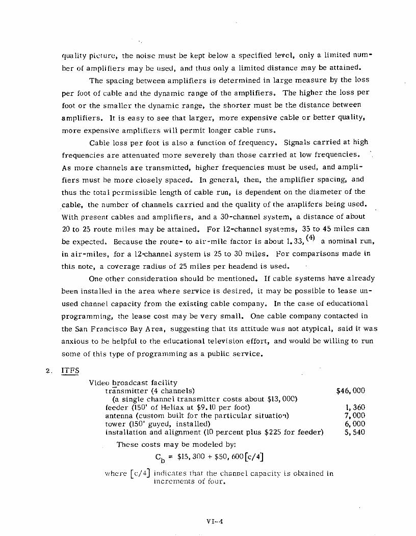
quality picture, the noise must be kept below a specified level, only a limited num-

ber of amplifiers may be used, and thus only a limited distance may be attained.

The spacing between amplifiers is determined in large measure by the loss

per foot of cable and the dynamic range of the amplifiers. The higher the loss per

foot or the smaller the dynamic range, the shorter must be the distance between

amplifiers. It is easy to see that larger, more expensive cable or better quality,

more expensive amplifiers will permit longer cable runs.

Cable loss per foot is also a function of frequency. Signals carried at high

frequencies are attenuated more severely than those carried at low frequencies.

As more channels are transmitted, higher frequencies must be used, and ampli-

fiers must be more closely spaced. In general, then, the amplifier spacing, and

thus the total permissible length of cable run, is dependent on the diameter of the

cable, the number of channels carried and the quality of the amnplifers being used.

With present cables and amplifiers, and a 30-channel system, a distance of about

20 to 25 route miles may be attained. For 12-channel systems, 35 to 45 miles can

be expected. Because the route- to air-mile factor is about 1.33,(4) a nominal run,

in air-miles, for a 12-channel system is 25 to 30 miles. For comparisons made in

this note, a coverage radius of 25 miles per headend is used.

One other consideration should be mentioned. If cable systems have already

been installed in the area where service is desired, it may be possible to lease un-

used channel capacity from the existing cable company. In the case of educational

programming, the lease cost may be very small. One cable company contacted in

the San Francisco Bay Area, suggesting that its attitude was not atypical, said it was

anxious to be helpful to the educational television effort, and would be willing to run

some of this type of programming as a public service.

2. ITFS

Video broadcast facilitytransmitter (4 channels) $46, 000

(a single channel transmitter costs about $13, 000)feeder (150' of Heliax at $9.10 per foot) 1, 360antenna (custom built for the particular situation) 7, 000tower (150' guyed, installed) 6, 000installation and alignment (10 percent plus $225 for feeder) 5, 540

These costs may be modeled by:

Cb = $15, 300 + $50, 600 [c/4]

where [c/4] indicates that the channel capacity is obtained inincrements of four.

VI-4

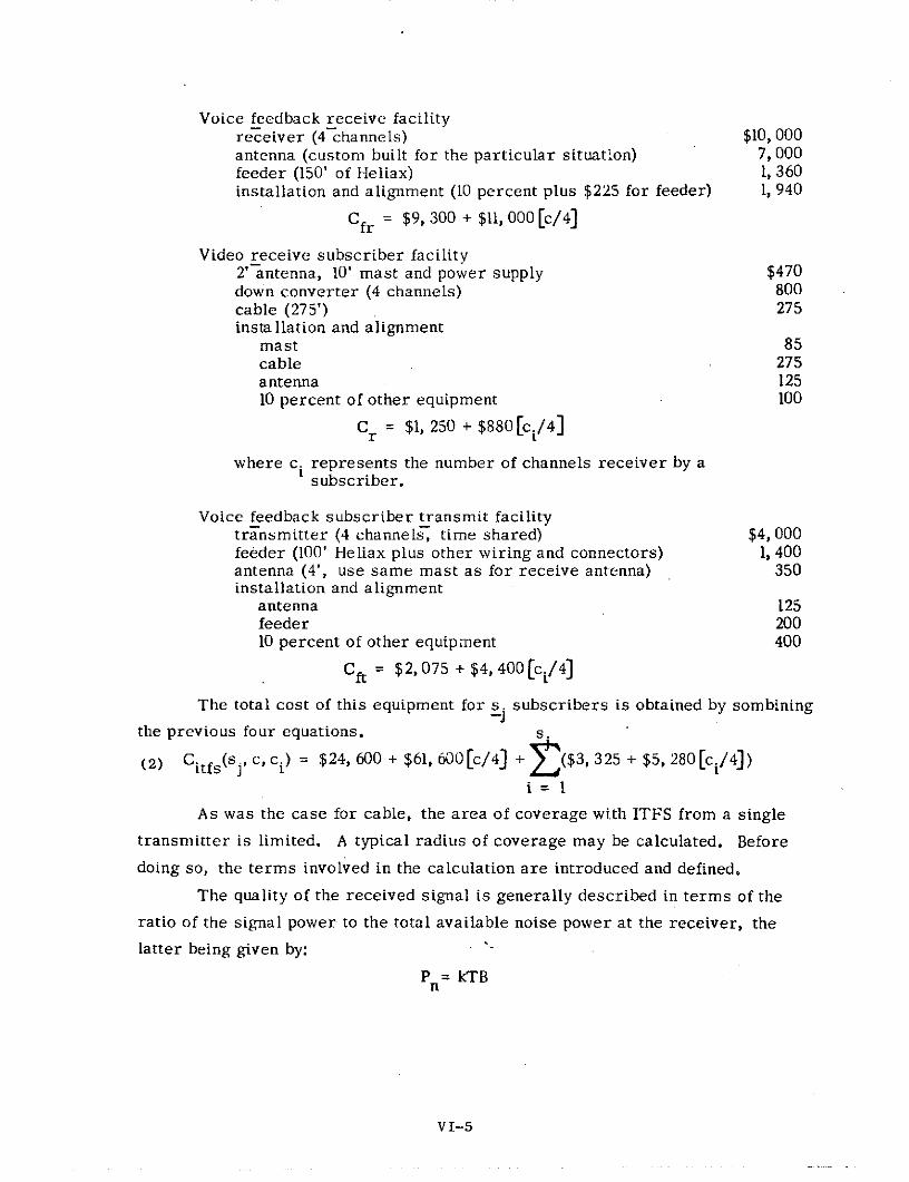
Voice feedback receive facilityreceiver (4 channels) $10, 000antenna (custom built for the particular situation) 7, 000feeder (150' of Heliax) 1, 360installation and alignment (10 percent plus $225 for feeder) 1, 940

Cfr = $9, 300 + $11, 000 [c/4]

Video receive subscriber facility2' antenna, 10' mast and power supply $470down converter (4 channels) 800cable (275') 275installation and alignment

mast 85cable 275antenna 12510 percent of other equipment 100

C r = $1, 250 + $880[ci/4]

where c. represents the number of channels receiver by a1 subscriber.

Voice feedback subscriber transmit facilitytransmitter (4 channels, time shared) $4, 000feeder (100' Heliax plus other wiring and connectors) 1, 400antenna (4', use same mast as for receive antenna) 350installation and alignment

antenna 125feeder 20010 percent of other equipment 400

Cft = $2, 075 + $4, 400 [ci/4]

The total cost of this equipment for s. subscribers is obtained by sombining-3

the previous four equations. s.

(2) Citfs(sj, c,c) = $24, 600 + $61, 600 [c/4] + 2($3, 325 + $5, 280 [ci/4])

i=l

As was the case for cable, the area of coverage with ITFS from a single

transmitter is limited. A typical radius of coverage may be calculated. Before

doing so, the terms involved in the calculation are introduced and defined.

The quality of the received signal is generally described in terms of the

ratio of the signal power to the total available noise power at the receiver, the

latter being given by:

P = kTBn

VI-5

where P is the received available noise powerk is Boltzmann's constantT is the effective receiver input noise temperature (OK)B is the receiver bandwidth

Signal transmission by radio waves between aligned antennas may be de-

scribed by the following equation:

Pr = PtGtG(4rd/)2

where Pr is the received signal power, in watts

Pt is the transmitted signal power, in watts

G t is the gain of the transmit antenna (a number ratio)

G r is the gain of the receive antenna (a number ratio)

d is the distance between the transmitting antenna and the receiveantenna, in feet

X is the wavelength of the transmitted signal carrier, in feet

With power and gain parameters now given in dB, the signal-to-noise ratio

(SNR) at the receiver input is:

SNR = 10 [log(Pr/P n)

= Pt + Gt + Gr - 20[log(47rd/)] - Pn

Using the maximum transmitter power allowed by the FCC of 10 watts per

channel, a broadcast antenna with 15 dB gain, and assuming a typical receiver noise

figure, F, of 10 and a receiver bandwidth of 6 MHz, we have:

Pt = 40 dBm (dBm is decibels with respect to 1 milliwatt)

G = 15 dB

X = 0.38 ft. (2.6 GHz)

T = (F - 1)T = (10 - 1) x 290K = 2610 OK

P = -198.6 dBm + 101.9 dB = -96.7 dBmn

Gr = 27. 5 dB (using a 4' receive antenna at 2. 6 GHz with 48 percentefficiency)

Then by substituting these values into the SNR formula,

SNR = 40 + 15 + 27.5 - 20 log(47r/X) - 20 log(d) + 96.7

Combining and rearranging terms,

20 log(d) = 148.-8 - SNR

In addition to the terms making up this last equation, we must include a

term to account for the random (statistical) occurrence of signal fading that ac-

companies any signal transmission through the atmosphere. Viewer surveys have

shown that if the no-fade nominal received SNR is 40 dB then satisfactory pictures

VI-6

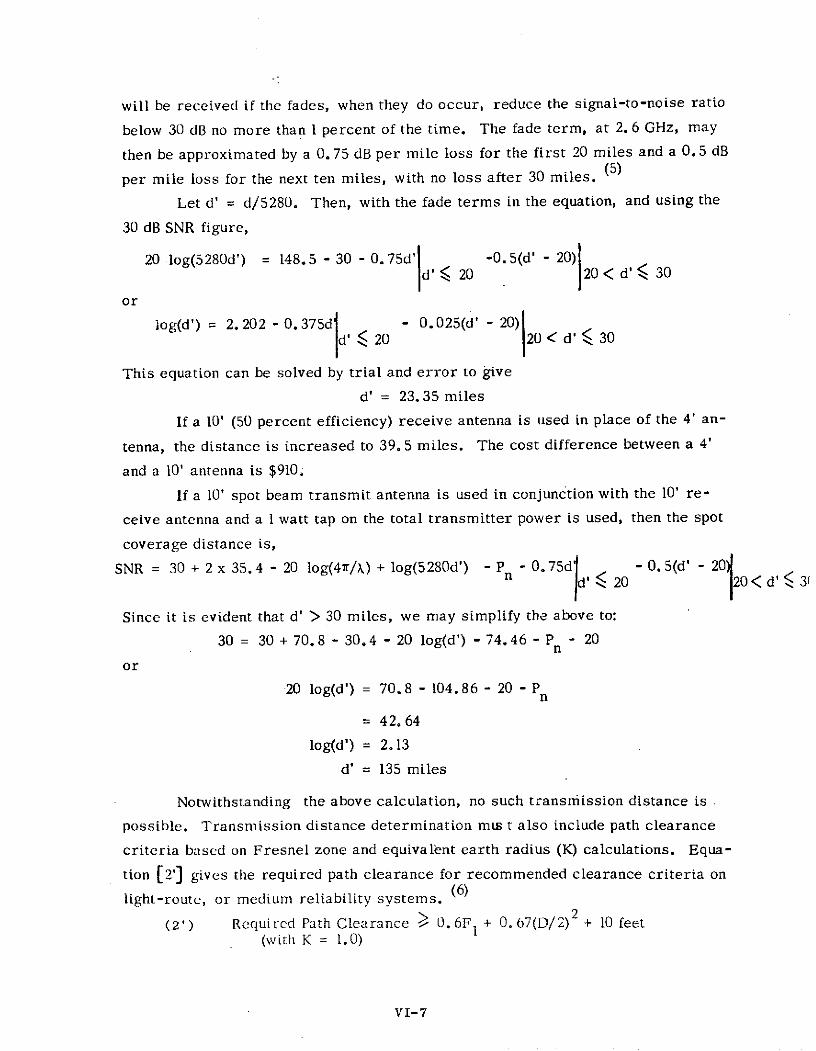
will be received if the fades, when they do occur, reduce the signal-to-noise ratio

below 30 dB no more than 1 percent of the time. The fade term, at 2. 6 GHz, may

then be approximated by a 0. 75 dB per mile loss for the first 20 miles and a 0. 5 dB

per mile loss for the next ten miles, with no loss after 30 miles. (5)

Let d' = d/5280. Then, with the fade terms in the equation, and using the

30 dB SNR figure,

20 log(5280d') = 148.5 - 30 -0. 75d' I -0.5(d' - 20)20< d' 30

or

log(d') = 2.202 - 0.375d 20 - 0.025(d' - 20) 20 < d' 30

This equation can be solved by trial and error to give

d' = 23. 35 miles

If a 10' (50 percent efficiency) receive antenna is used in place of the 4' an-

tenna, the distance is increased to 39. 5 miles. The cost difference between a 4'

and a 10' antenna is $910.

If a 10' spot beam transmit antenna is used in conjunction with the 10' re-

ceive antenna and a I watt tap on the total transmitter power is used, then the spot

coverage distance is,

SNR = 30 + 2 x 35.4 - 20 log(47r/X) + log(5280d') - P - 0.75d '< - 0.5(d' - 20 <d

Since it is evident that d' > 30 miles, we may simplify the above to:

30 = 30 + 70.8 - 30.4 - 20 log(d') - 74.46 - Pn - 20

or

20 log(d') = 70.8 - 104.86 - 20 - Pn

= 42.64

log(d') = 2.13

d' = 135 miles

Notwithstanding the above calculation, no such transmission distance is

possible. Transmission distance determination mts t also include path clearance

criteria based on Fresnel zone and equivalent earth radius (K) calculations. Equa-

tion [2'] gives the required path clearance for recommended clearance criteria on

light-route, or medium reliability systems. (6)

(2') Required Path Clearance > 0. 6F + 0.67(D/2) 2 + 10 feet(with K = 1.0)

VI-7

where K is the earth radius factor

Fl is the radius of the first Fresnel zone, in feet, and is given by:

F I = 72.1 x (dd 2/fD)1/ 2

where d I = the distance from one end of the path to thepoint of reflection

D = the total path length

d2= D - dlf = the frequency in GHz

In Figure 1, the mid-path clearance as given by equation [2'] is plotted

against the path length in miles. This path clearance is not the height at which the

radio path must be maintained above ground. Rather, as the name implies, it is

a distance which must be maintained above the top of any ground structures such

as buildings or trees. Even without allowing for the required increases in path

clearance that would account for ground structures, the clearance height places

prohibitive requirements on antenna heights for distances beyond 40 miles, unless

the transmitting antenna can be located on a nearby mountain, In this case, of course,

extra expense will be incurred in transmitting the signal to the mountain. It has been

assumed in this report that the coverage area for ITFS will be limited to 25 miles

from any one transmitter, with possible special beams reaching subscribers up to

40 miles away.

C. Point-To-Point Systems Equipment

1. Cable

The cost of a point-to-point cable system is obtained in a manner quite

similar to that for a wide-area cable system. The difference is that no costs per

subscriber need be included. The result is:

(3) Cca(c, m) = $5, 200m + $1, 60 0 c (assuming only 5 percent is underground)

where m is the number of cable-miles in a point-to-point run.

2. ITFS

Video transmit terminal with audio receive

The cost of a video point-to-point transmit terminal with audio receivewill be the same as for the wide-area broadcast terminal if we replacethe two wide-area antennas with directional antennas (assume 6' antennasare used at a cost of $420 each). Thus, using previously established no-menclature, with a prime to indicate point-to-point costs:

C b = $8.060 + $50, 600 [c/4] and Cr = $2, 060 + $11, 000 [c/4]

VI-8

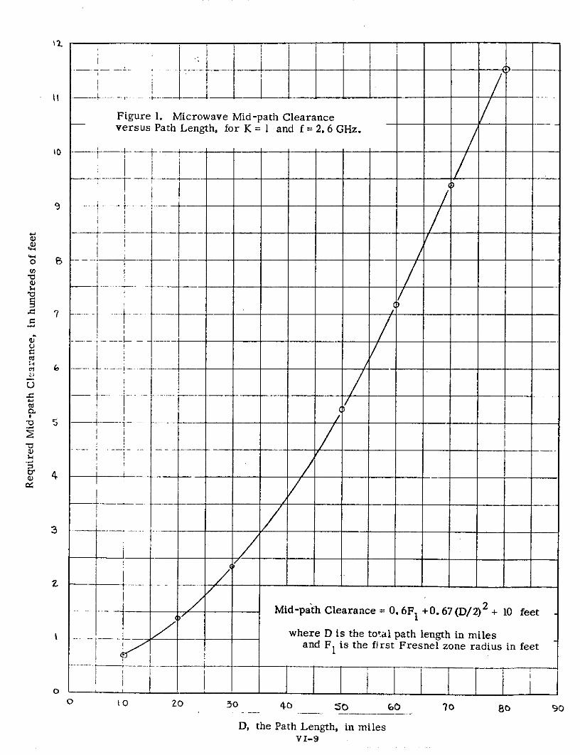
Figure 1. Microwave Mid-path Clearanceversus Path Length, for K = 1 and f = 2. 6 GHz.

o *----- .-----

IU .. . ... ~ -- r--- -

VI-9

' I

4- -- --

_

-- . ...

, ------__-

....

-o

4.. . . .-- _ . .i ......

1--

VI-9

Repeater stationtower (150' guyed, installed) $6, 000four 6' parabolic antennas 1, 700receiver and transmitter (4 channels) 41, 000estimate of voice talk-back receiver/transmitter 7, 000feeder (400' of Heliax) 3, 650batteries and chargers 1, 000 plus

200 / channelinstallation and alignment (10 percent plus $1, 300 • 6, 050

for Heliax)

Crep = $21, 300 + $45, 300 [c/4]

Video receive terminal with audio transmitvoice feedback transmitter (4 channel, time shared) $4, 000receive antenna and transmit antenna (two, 6') 840transmit feeder (150' of Heliax) 1, 360receive feeder (150' of Heliax) 1, 360tower (not necessary if ITFS wide-area transmission is 6, 000

the next step -- the same tower may be used)down converter (4 channels) 800installation and alignment

antennas 500feeder 45010 percent of other equipment 480

C' = $1, 360 + $420 + $225 + $250 + $880 [c/4]r

= $2, 255 + $880 [c/4]

C = $2, 255 + $4, 400 [c/4] + $6, 000

The total cost formula for ITFS point-to-point transmission is obtained by

combining the above.

Citfs(c, R) = $14, 630 + $66, 880 c/4] + $6, 000 + ($21, 300 + $45, 300 [c/4]) x R

where R is the number of repeaters.

2. Microwave

Transmit or receive terminalradio (per channel) $4, 500antenna and feed 1, 900batteries and charger - first channel 1, 600

each additional channel 200tower (150' guyed) 6, 000installation and alignment - first channel 1, 000

each additional channel 500

VI-10

voice feedbackradio 4, 500antenna and feed 1, 900batteries and charger 200multiplex: heavy route - per channel 2, 000

light route - per channel 1,000installation and alignment - first channel 900

each additional channel 200

Cmt = $24, 500 + $7, 400(c - 1) heavy route voice system

C $23, 500 + $6, 400(c - 1) light route voice systemmt

Repeaterradio - first channel $7,000

each additional channel 7,000antennas and feed 3, 800batteries and charger - first channel 2, 000

each additional channel 200tower (150' guyed) 6, 000installation and alignment - first channel 1, 300

each additional channel 500voice feedback

radio 7,000antennas and feed 3, 800batteries and charger 200installation and alignment 1, 100

C = $32, 200 + $7, 70 0 (c - 1)mr

The total cost formula for microwave point-to-point transmission is:

Cm(c, R) = $49, 000 + $14, 800(c - 1) + $32, 200 + $7, 700(c - 1) x R

where R is the number of repeaters.

VI-11

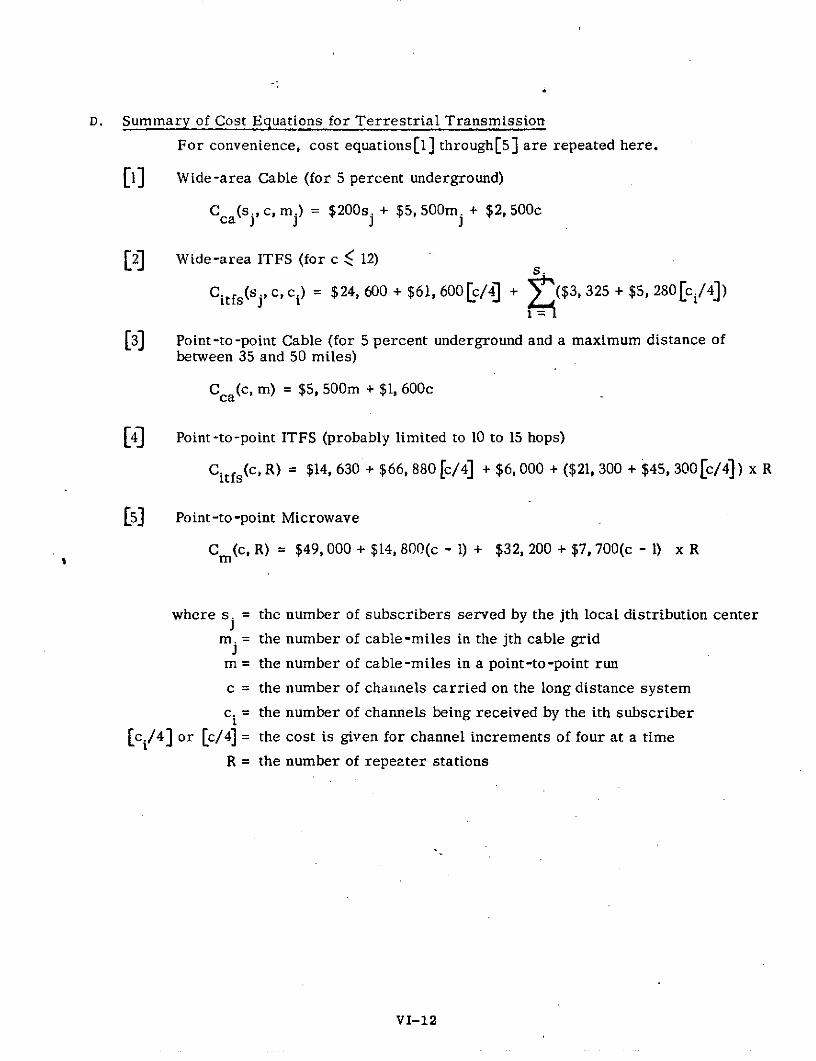
D. Summary of Cost Equations for Terrestrial Transmission

For convenience, cost equations[l] through[5] are repeated here.

[1] Wide-area Cable (for 5 percent underground)

Cca(s C, c, m) = $200s. + $5, 500m. + $2, 500c

[2] Wide-area ITFS (for c < 12)

Citfs(s, c, c) = $24, 600 + $61, 600 [c/4] + ($3, 325 + $5, 280 [ci/4])

[3] Point-to-point Cable (for 5 percent underground and a maximum distance ofbetween 35 and 50 miles)

Cca(c, m) = $5, 500m + $1, 600c

[4] Point-to-point ITFS (probably limited to 10 to 15 hops)

Citfs(c, R) = $14, 630 + $66, 880 [c/4] + $6, 000 + ($21, 300 + $45, 300[c/4]) x R

[5] Point-to-point Microwave

Cm(c, R) = $49, 000 + $14, 800(c - 1) + $32, 200 + $7, 700(c - 1) x R

where s. = the number of subscribers served by the jth local distribution center

m. = the number of cable-miles in the jth cable grid

m = the number of cable-miles in a point-to-point run

c = the number of channels carried on the long distance system

ci = the number of channels being received by the ith subscriber

[ci/4] or [c/4] = the cost is given for channel increments of four at a time

R = the number of repeater stations

VI-12

E. REFERENCES

1. Cosgrave and Chipp, "Economic Considerations For Communication Systems",

IEEE Trans. on Comm. Tech., 16:513-525, August, 1968

2. Comanor and Mitchell, "Cable Television and the Impact of Regulation",

The Bell Journal of Economics and Management Science, 2:154-212, Spring, 1971.

3. D.A. Dunn, "Cable Television Delivery of Educational Services", IEEE Eascon

'71 Record, pp. 157-163. (The IEEE Eascon Conference was held in Washington,

D.C., October 6, 7, 8, 1971)

4. Davis and Lally, "Systems Engineering Survey of Subscriber Loop Plant",

IEEE Trans. on Comm. Tech. 19:71-79, February, 1971.

5. Conversation with Mr. Jim Talmadge of Genesys Systems, Mountain View, Calif.

6. Engineering Staff of Lenkurt Electric Co., Inc., Engineering Considerations

For Microwave Communications Systems, Lenkurt Electric Co., Inc., San Carlos,

Calif., June, 1970.

VI-13

CHAPTER vii

LEAST-COST COMPARISONOF

ALTERNATIVE TELECONFERENCING SYSTEMS

A. Introduction

The teleconferencing system envisioned in this report may be modeled in

terms of the natural division between long-distance transmission and local dis-

tribution. Happily, these two subsystems are almost completely decoupled in the

sense that the least expensive total system may be determined by separate analyses

for each subsystem. Drawing on material presented in chapters five and six, this

chapter develops the models used for each subsystem, outlines the methods used

in the comparisons, and gives the results obtained.

B. Long-Distance Transmission Subsystems

The long-distance subsystem consists of the means by which the teleconfer-

encing signals are transmitted from the origination station or stations to the local

distribution centers. Two types of long-distance subsystem are considered: a sat-

ellite with earth stations at or near each local distribution center and a terrestrial

microwave network. The following analysis accounts for only the first order costs

of both systems. Nevertheless, the results obtained seem so favorable to the use

of a satellite for regional teleconferencing that a more exhaustive analysis at this

juncture was not indicated. Af,

1. Models and Cost Equations

a. The Terrestrial Microwave Network

For the moment, suppose there is only one origination station. A micro-

wave network would then consist of a chain of repeater stations connecting each

city to be served. Each repeater would transmit TV program signals away fromthe origination point and audio signals towards the origination point. A very highquality TV signal would have to be maintained at each repeater inasmuch as thesignal received by the local distribution center at the ends of the chain would passt hrough several repeaters.

A microwave terminal station (no retransmission of the video signal isrequired) would only be used in the network at the ends of the chain. Nevertheless,each terminal station will have its video transmit counterpart somewhere upstream

VII41

towards the origination station. This is significant in that it allows the costs ofthe microwave system to be modeled as the total number of stations used, whether

terminal or repeater, times the cost of a repeater station; or, in equation form,

(1) Cldm(c. N) = [I + 1(N)]NCr(c)

where Cldm(c , N) is the cost of the long-distance microwave networkc is the video channel capacity of the network

N is the number of cities being served by the networkn (N) is the ratio of the number of microwave repeater stations

between cities to the number of cities connected by thenetwork

Cr(c) is the cost of a microwave repeater station

While the values for both N and Cr may readily be determined, q can beknown accurately only after a preliminary route survey with topographic mapsand path porffles has been completed. It is sufficient for present purposes, how-ever, to derive a rough estimate of the functional dependence of nj on N. A uniformdistribution of cities throughout the entire area to be served is assumed. Althoughnot a very likely distribution for an actual system, it might be argued that the num-

ber of repeaters required to serve such a distribution could be considered as an

upper bound since any departure from uniformity would allow advantage to be takenof the clustering that would appear. If it is further assumed that the origination

station will be located at one of the N cities to be served, the straight-forward deri-vation of ?(N) is as follows.

Consider a region of rectangular shape L miles long by W miles wide. Fora uniform distribution, each city will be at the center of a smaller rectangle thatis L/N 1/2 miles long by W/N 1/ 2 miles wide (see Figure 1). The intercity separation

distance is thus either L/N1/2 miles (long link) or W/N 1/ 2 miles (short link) depend-ing on whether the direction of travel is parallel to the length or the width of the rec-tangle. If, insofar as possible, cities are connected to their neighbors using shortlinks fewer intercity repeaters will be required than with any other link pattern.With this pattern, the network will consist of (N 1/2 - 1)N1/ 2 short links and (N1/2 - 1)long links.

In calculating the total number of intercity repeaters implied by this pattern,let h represent the average inter-repeater (hop) distance and D represent the dis-tance between cities, or the link length. Because h is the average hop distance and

VII-2

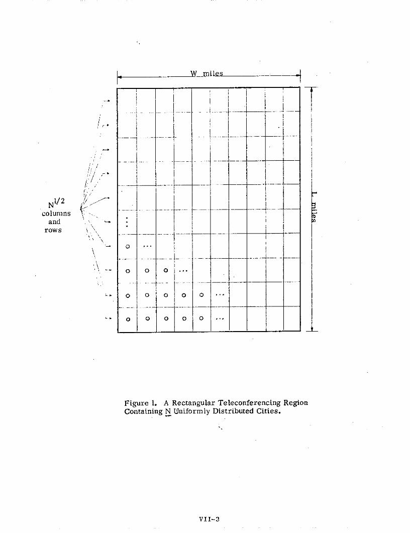
W miles

-1--fl

r ___

.............-- ""- --- ---

1/2 /Ncolumns

TOWS \-**- 1 4-4and " ISrows

\ 0

ol o 0 o .

L 0

Figure 1. A Rectangular Teleconferencing RegionContaining N Uniformly Distributed Cities.

VII-3

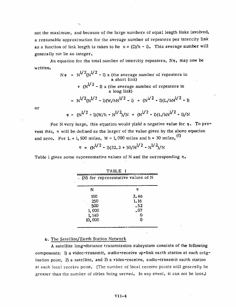
not the maximum, and because of the large numbers of equal length links involved,

a reasonable approximation for the average number of repeaters per intercity link

as a function of link length is taken to be n = (D/h - 1). This average number will

generally not be an integer.

An equation for the total number of intercity repeaters, N1, may now be

written.

N 7 = NI/ 2 (N1/ 2 - 1) x (the average number of repeaters ina short link)

+ (N1/2 - 1) x (the average number of repeaters ina long link)

= N1/ 2 (N1/ 2 - 1)(W/hN 1/ 2 - 1) + (N1/ 2 - 1)(L/hN1/ 2 - 1)

or

7 = (N 1/ 2 - l)(W/h - N 2)/N + (N1/ 2 - 1)(L/hN1/2 - 1)/N

For N very large, this equation would yield a negative value for n. To pre-

vent this, n will be defined as the larger of the value given by the above equation

and zero. For L = 1, 500 miles, W = 1, 000 miles and h = 30 miles, (1)

17 = (N1/2 - 1)(32.3 + 50/N 1/2 - Nl1/2 )/N

Table 1 gives some representative values of N and the corresponding r.

TABLE 1

(N) for representative values of N

N 7

100 2.46250 1.16500 .52

1,000 .071, 140 0

10,000 0

b. The Satellite/Earth Station Network

A satellite long-distance transmission subsystem consists of the following

components: 1) a video-transmit, audio-receive up-link earth station at each orig-

ination point, 2) a satellite, and 3) a video-receive, audio-transmit earth station

at each local receive point. (The number of local receive points will generally be

greater than the number of cities being served. In any event, it can not be less.)

VII-4

Two types of video-receive earth stations might be distinguished according

to their output signal-to-noise ratio. Earth stations that feed local distribution

subsystems would need a higher output signal-to-noise ratio than would earth sta-

tions that serve isolated subscribers (no further distribution is necessary). For

simplicity, the following analysis assumes that all earth stations provide the same

higher quality signal as that required for redistribution. A slight cost savings could

be realized in any actual implementation by limiting use of the higher quality sta-

tion to receiving points that actually require the higher quality signal. In the com-

parison of local sa bsystems later in this chapter, allowance will be made for this

savings.

The cost of the long-distance transmission subsystem by satellite may be

expressed as:

(2) Clds(c, N) = Cs(c, N) + Cb(c, N) + NCe(c, N)

where C ds(c, N) = the cost of the long-distance satellite subsystem

c = the number of video channels carried by the satellite

N = the minimum number of video-receive earth stationsin the network

Cs(c, N) = the cost of that part of the space segment of thesatellite subsystem actually used by the telecon-ferencing system

Cb(c, N) = the cost of the master video-transmit, audio-receivestation(s)

Ce(c, N) = the cost of a video-receive, audio-transmit earthe station

2. Cost Summaries

The costs for long-distance subsystems are given in detail in chapters five

and six. The pertinent results of these chapters are summarized and placed here

for convenient reference together with additional explanatory material relating to

their use.

a. Satellite Cost Summary

The earth station costs that are presented in chapter five are based on the

assumption that the cost per watt per year of satellite power is known. Earth sta-

tion costs are then calculated using the criterion of minimum overall satellite sys-

tem cost. Thus, if the cost per watt-of-space-segment-use increases, minimizing

VT T-_

total system cost would require that the earth stations be made more sensitive, and

consequently more costly, so that less satellite power need be used. Similarly, if

only a few earth stations are to be constructed, their unit cost should be rriuch higher

than if many are needed.

The range of per-watt space-segment charges that is used in chapter five is

developed in chapter four. It is based on matching in-orbit satellite capacity with

various assumed demand curves over time for that capacity. The present worths

of the costs that would be incurred in providing sufficient satellite capacity to just

meet these demands are calculated using the costs of currently proposed satellites.

Then the amount that must be charged for a watt-year of satellite capacity is deter-

mined such that the present worths of the revenue streams associated with each de-

mand curve are equal to the present worths of the costs, respectively, of satisfying

the demand. The range of charges runs from $15, 000 per watt-year to $50, 000 per

watt-year. From chapter five, then, a satellite system capable of one-way video

and return audio from any earth station in a region approximately 1, 500 miles by

1, 000 miles would incur costs as a function of N as shown in Tables 2 through 7

(Cw/y is the cost to the teleconferencing system of one watt of satellie power -- fr

one year).

As explained in chapter five, the earth station costs include the following.

1) equipment costs

2) site costs (assumed to be 40 percent of the antenna costs)

3) installation costs (assumed to be 10 percent of the equipment costs)

4) the present worth of maintenance costs over an assumed 25-yearlifetime using a discount rate of 10 percent. (Annual maintenancecosts are assumed to be 15 percent of equipment costs.)

5) the cost of channel separation and demodulation to baseband for eachvideo channel received. _On a per-channel basis, this cost has beenestimated to be near $1, 200, as follows. A lower bound may be es-timated by looking at the function and cost of an ITFS down converter.The down converter, used with an ITFS receive-station, does no morethan shift the frequency of the incoming rf sighal down to the properTV carrier frequency, using a double conversion process, and thenamplifies the result. The cost of the down converter is $800. Demodu-lation is not included (it, of course, is not necessary in ITFS trans-missions). An upper bound may be taken to be $1, 500. This is thecost of the equipment needed at a cable headend site to prepare a TVsignal, received from a microwave link, for transmission ofi the cable. (2)This $1, 500 does not include demodulation either, but does include AMmodulation, frequency translation to the proper cable channel, and

VII-6

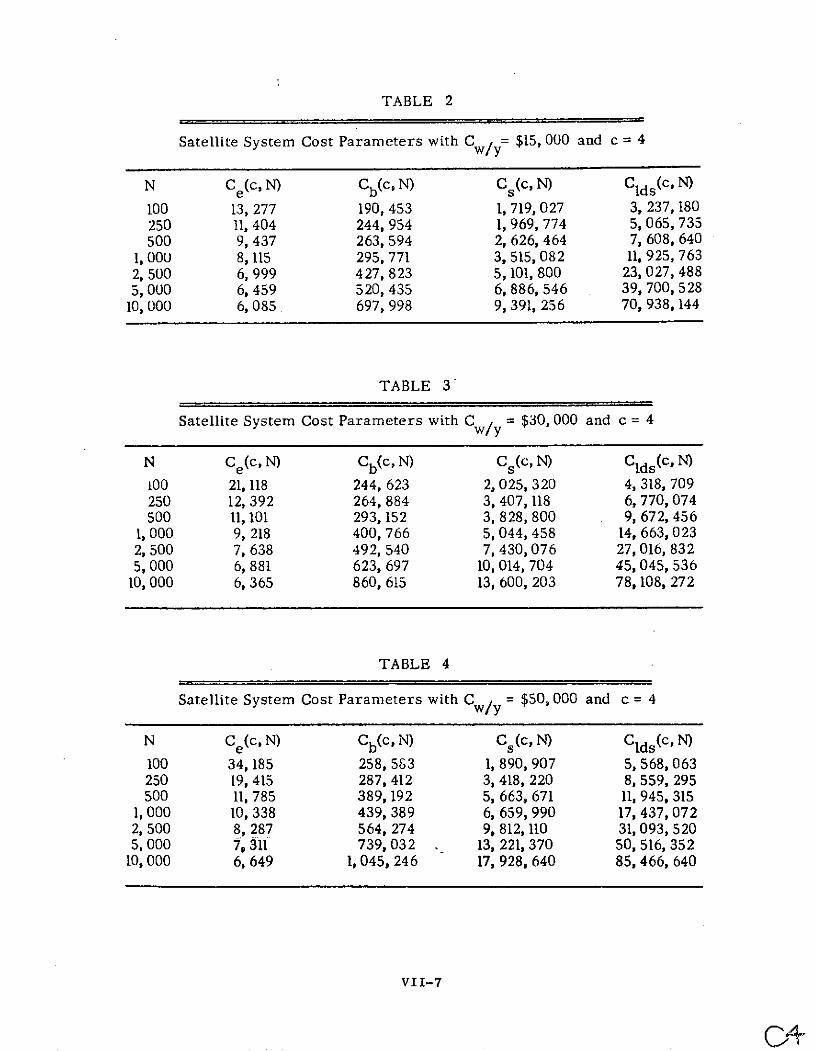
TABLE 2

Satellite System Cost Parameters with Cw/y= $15, 000 and c = 4

N Ce(c, N) Cb(c, N) Cs(c, N) Clds(c, N)

100 13, 277 190, 453 1, 719, 027 3, 237,180250 11, 404 244, 954 1, 969, 774 5,065,735500 9, 437 263, 594 2, 626, 464 7, 608, 640

1, 000 8, 115 295, 771 3, 515,082 11, 925, 7632, 500 6, 999 427, 823 5,101, 800 23, 027,4885, 000 6, 459 520, 435 6, 886, 546 39, 700, 528

10, 000 6, 085 697, 998 9, 391, 256 70, 938, 144

TABLE 3

Satellite System Cost Parameters with Cw/y = $30, 000 and c = 4

N Ce(c, N) Cb(c, N) Cs(c, N) Clds(c, N)

100 21, 118 244, 623 2, 025, 320 4, 318, 709250 12, 392 264, 884 3, 407, 118 6, 770, 074500 11, 101 293, 152 3, 828,800 9, 672, 456

1, 000 9, 218 400, 766 5, 044, 458 14, 663, 0232, 500 7, 638 492, 540 7, 430,076 27,016, 8325,000 6, 881 623, 697 10, 014, 704 45, 045, 53610,000 6, 365 860, 615 13, 600, 203 78, 108, 272

TABLE 4

Satellite System Cost Parameters with Cw/y = $50, 000 and c = 4

N Ce(c, N) Cb(c, N) Cs(c, N) Clds(c, N)

100 34, 185 258, 583 1, 890, 907 5, 568, 063250 19, 415 287, 412 3, 418, 220 8, 559, 295500 11, 785 389, 192 5, 663, 671 11, 945, 315

1, 000 10, 338 439, 389 6, 659, 990 17, 437, 0722, 500 8, 287 564, 274 9, 812, 110 31, 093, 5205, 000 7, 311 739, 032 13, 221, 370 50, 516, 35210, 000 6, 649 1, 045, 246 17, 928, 640 85, 466, 640

VII-7

/4-.

TABLE 5

Satellite System Cost Parameters with Cw/y $15, 000 and c 12

N C (c, N) Cb(c, N) Cs(c, N) C1ds(c, N)

100 44, 205 328, 056 3, 083, 475 7, 832, 028250 28, 173 3541861 5, 168,194 12, 566, 348500 24, 865 457, 012 6, 227, 586 19, 117, 216

1, 000 21, 722 506, 487 8, 287,900 30, 516, 7202, 500 19, 078 739, 824 12, 093,080 60, 527, 1045,000 17, 832 919, 098 16, 257, 658 106, 335, 184

10, 000 16, 980 1, 248, 249 22, 008, 800 193, 059, 920

TABLE 6

Satellite System Cost Parameters with Cw/y = $30, 000 and c 12

N C (c, N) Cb(c, N) Cs(c, N) CIds(c, N)

100 68, 250 354, 861 3, 418, 916 10, 598, 739250 41, 094 460, 870 6, 113, 468 16, 847, 920500 27, 071 614, 462 10, 116, 378 24, 266, 496

1, 000 24, 318 689, 948 11,992, 616 37,000, 1122, 500 20, 606 877, 653 17,622, 336 70, 051, 7605, 000 18, 844 1, 140, 515 23, 679, 872 119, 038, 928

10,000 17, 650 1, 601, 609 31, 992, 640 210, 097, 520

TABLE 7

Satellite System Cost Parameters with C w/y $50, 000 and c = 12

N Ce(c, N) Cb(c, N) Cs(c, N) Cids(c, N)

100 81, 443 450, 293 5, 032, 237 13, 676, 797250 41, 094 606, 186 9, 968, 821 20, 848,576500 38,959 669, 417 10, 121, 574 30, 270, 368

1, 000 26, 058 773, 462 17, 017, 984 43, 849, 0402, 500 22, 161 1, 030, 177 23, 275, 408 79, 706, 9125,000 19,873 1, 386, 146 31, 278, 336 132, 027, 90410,000 18,332 1, 997, 533 42, 237, 200 227, 550, 608

:VII-8

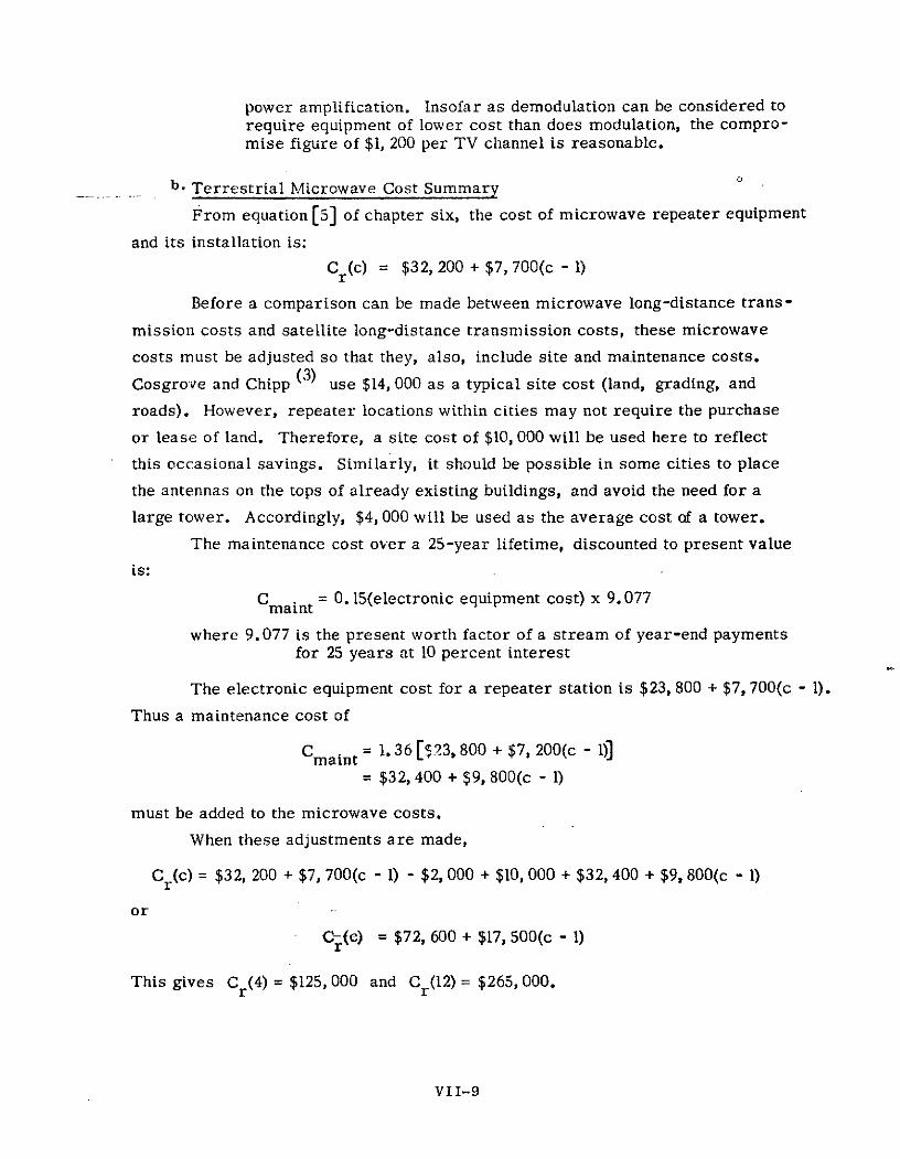
power amplification. Insofar as demodulation can be considered torequire equipment of lower cost than does modulation, the compro-mise figure of $1, 200 per TV channel is reasonable.

b. Terrestrial Microwave Cost Summary

From equation [5] of chapter six, the cost of microwave repeater equipment

and its installation is:

Cr(c) = $32, 200 + $7, 700(c - 1)

Before a comparison can be made between microwave long-distance trans-

mission costs and satellite long-distance transmission costs, these microwave

costs must be adjusted so that they, also, include site and maintenance costs.

Cosgrove and Chipp (3) use $14, 000 as a typical site cost (land, grading, and

roads). However, repeater locations within cities may not require the purchase

or lease of land. Therefore, a site cost of $10, 000 will be used here to reflect

this occasional savings. Similarly, it should be possible in some cities to place

the antennas on the tops of already existing buildings, and avoid the need for a

large tower. Accordingly, $4, 000 will be used as the average cost of a tower.

The maintenance cost over a 25-year lifetime, discounted to present value

is:

C maint = 0. 15(electronic equipment cost) x 9.077

where 9.077 is the present worth factor of a stream of year-end paymentsfor 25 years at 10 percent interest

The electronic equipment cost for a repeater station is $23, 800 + $7, 700(c - 1).

Thus a maintenance cost of

Cmaint = . 36 [$23, 800 + $7, 200(c - 1)]= $32, 400 + $9, 800(c - 1)

must be added to the microwave costs.

When these adjustments are made,

Cr(c) = $32, 200 + $7, 700(c - 1) - $2, 000 + $10, 000 + $32, 400 + $9, 80 0 (c - 1)

or

Cr(c) = $72, 600 + $17, 500(c - 1)

This gives Cr(4) = $125, 000 and Cr(12) = $265, 000.

VII-9

C. Long-Distance Subsystem Comparison

The comparison is based on equations [1] and [2] . With the values of the

cost parameters as given in the previous section, both equations have been-

plotted in Figures 2 and 3 as a function of N with Cw/y as a parameter. Figure 2

gives the costs for systems that carry four video channels and figure 3 gives the

costs for 12-channel systems. Each figure also includes a plot of what the microwave

network would cost if r7 (N) = 0. This approximates the case where the cities involved

are not spread throughout an entire region but are, in fact, so situated that very few

intercity repeaters would be needed.

It may be seen that for any regional network serving even as few as 100 cities

the satellite/earth station network is dramatically less expensive than the terres-

trial microwave network. In fact, providing 12 channels via the satellite is less

costly than providing 4 channels with the microwave network, even though to provide

12 channels through the satellite involves stacking the TV channels so close together

in frequency that adjacent channels must be transmitted on carriers that are cross-

polarized with respect to each other (permitting some overlapping occupancy of the

available frequency spectrum) and the earth stations must then be equipped with two

antennas and two preamplifiers. A microwave system would become less expensive

for service to some number of cities less than 100 (about 30 to 50 if the curves are

extrapolated) if they were not spread throughout several states as in the above case.

In view of this cost dependency on the number of cities involved, one is led

to ask how many cities might require service in a typical regional system. An ex-

ample of a region that might actually be served by a teleconferencing system is the

Rocky Mountain region. In the eight states of Lhis region there are 1168 cities. There

are 361 cities of greater than 2, 000 population and 100 cities of greater than 10, 000

population. (The breakdown by states is given in Appendix F) A teleconferencing

system transmitting continuing professional education material, would be of most

use in the smaller cities where large or specialized libraries and other research

facilities are not available. Thus, most of the 361 cities of greater than 2, 000 pop-

ulation would probably wish service. This is an obvious case, then, of where the

satellite system would be less expensive.

Of course, one reason that a terrestrial microwave network is more ex-

pensive is that each receive-station in the network must also be a relay station

(that is, a repeater), and only slight degredation of signal quality can be tolerated

VII-10

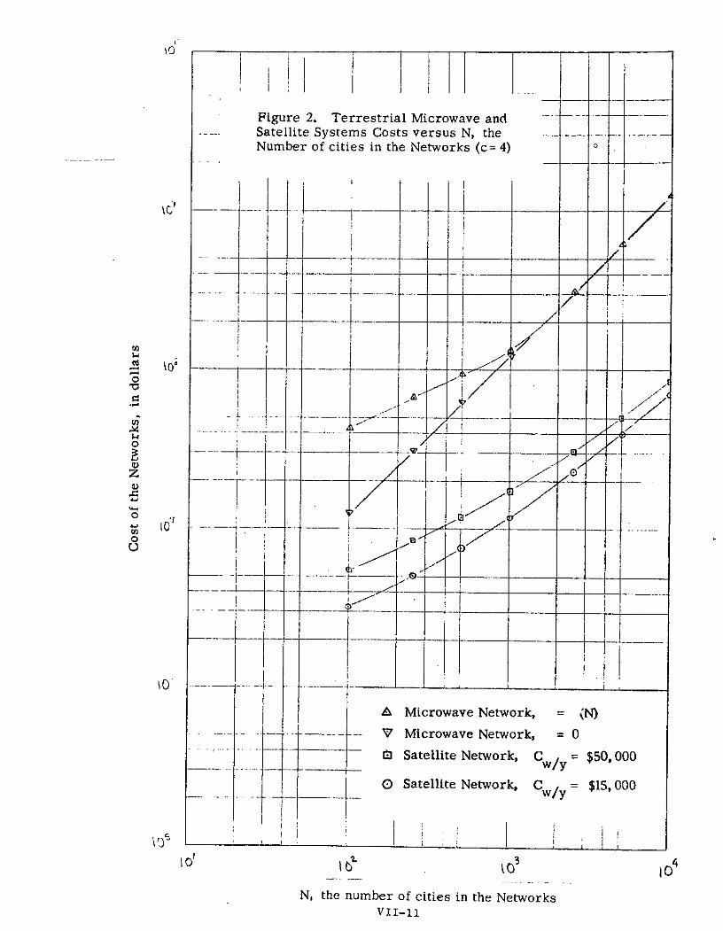
Figure 2. Terrestrial Microwave andSatellite Systems Costs versus N, theNumber of cities in the Networks (c= 4)

----- K-- - 1\Ii

to-

U)T

S_ _ I

o w/

-_ __10" .. . . . "

\O I-- ------ ~------- -j; _

N, the number of cities in the Networks

VII1 [0 Satellite Network, C = $15, 000

N, the number of cities in the NetworksVI!-II

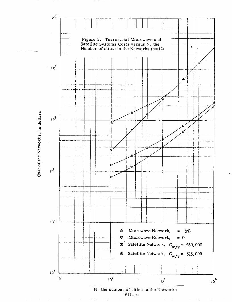
1 i I I I. . . ..I

Figure 3. Terrestrial Microwave andSatellite Systems Costs versus N, theNumber of cities in the Networks (c= 12)

-- --t

0 T

E--Satellite Network, C = $50, 000

... .

..... ..-... ..i -. .. ....--- - --- "

- W-

A Microwave Network, = (N)---- .. .. - V Microwave Network, = 0

... " Satellite Network, CY = $50, 000

0 Satellite Network, C /y $15, 000

L ' ;I1 o /

N, the number of cities in the NetworksVII-12

at each repeater and still preserve an acceptable quality for subscribers at the ex-

treme downstream ends of the network. By comparison, a satellite network has

only one repeater in the whole network. An earth station need have only TV-receive

capability plus audio transmit equipment and is, therefore, less costly than a re-

peater by at least the cost of the TV retransmit and the audio receive equipment.

In addition, line-of-sight operation from the satellite is generally possible without

the use of expensive towers.

It might also be argued that earth stations serving small cities need not be

concerned about standby power. If the city power fails, no one could watch tele-

vision anyway, and since the earth station is not one link in the chain of stations

providing service to cities further on, the need for reserve power does not exist.

D. Local Distribution Subsystems

With the acceptance of a satellite and an earth-station network as the least-

cost method of long-distance transmission for a regional teleconferencing system,

three presently available technologies may be considered in the synthesis of the

local distribution subsystem: ITFS, cable, and signal reception at subscriber pre-

mises using a low-cost earth station. * Each is most appropriate for slightly dif-

ferent subscriber demographics. (Happily, however, cable and ITFS do have

roughly the same range of coverage from one headend or transmitter, making di -

rect comparison a bit less cumbersome.) Cable, because of the high cost per mile

of installation, is best suited to fairly dense subscriber populations. For instance,

most commercial cable ventures regard 40 potential subscribers per route-:nile of

cable as a minimum requirement for successful financial operation. If all subscribers

*As mentioned above, in terms of teleconferencing programs for continuing profes-sional education, the professionals in the smaller cities, without specialized libra-ries and dedicated research facilities, stand to benefit the most by their reception.In many of these smaller cities, or equivalently, in a large percentage of all thecities being served, there are fewer than 10 professionals in any one discipline whocould be considered as potential subscribers. Having practically no need to redis-tribute the signal from the single long-distance earth station reception point, suchcities would be in the market for a minimal G/T earth station at the lowest possiblecost." The predominance in number of the small city is,. then, a dominant consider-ation in earth-station cost determination. Consequently, this study assumes thatreception by low-cost earth stations will be planned from the beginning.

VII-13

were uniformly spaced over the local distribution area, 40 subscribers per route-

mile would be equivalent to approximately 500 subscribers per square mile. **

ITFS, in contrast, because of the relatively high cost of subscriber terminals

in comparison with cable subscriber drops, finds application where subscribers are

widely dispersed. The ITFS system now in use by the Association for Continuing

Education, with studio-classrooms at Stanford University, is a good example. This

system serves about 21 subscriber receive-points scattered throughout the entire

San Francisco Bay area.

Reception at a subscribers premises via a low-cost earth station has, of

course, the same advantages as ITFS for dispersed subscriber populations without

the need for an intermediate transmitter.

These technologies are not mutually exclusive and will most often be used

to complement one another in providing signal distribution within any given commun-

ity. An exception would be that ITFS and low-cost earth stations would only rarely

be used simultaneously because of their very similar characteristics. Consequently,

there are only two main local system configurations that could occur. Given their

costs, which one is selected depends on the location of subscribers. They are:

A. A single earth station for long-distance reception used in con-junction with an ITFS transmitter. The ITFS receivers wouldsupply the signal both to cable headends and to isolated sub-scribers.

B. One or more earth stations each serving either a cable headendor a single subscriber.

** This number was obtained in the following manner. For a uniform subscriberpopulation of P per square mile, subscribers are assumed to be at the intersection

points of a cartesian grid, with P1/2 lines per mile, that may be imagined to covereach square mile. The average subscriber drop-cable run is from 100 to 150 feet.Therefore, a distribution cable-run would be required along each line of the griduntil the subscriber density is high enough that two adjacent grid lines are no morethan 300 feet apart. When that occurs, two grid lines could be served by one dis-tribution cable.

All such cable runs would be connected by one perpendicularly run trunkline. Thus, the total number of cable-miles per square mile of service area would

be (Pl/2/2 + 1) with each cable-run serving two grid lines. Although each cable run

is one mile long and each would serve 2P1/2 subscribers, 2P 1/ 2 must be slightlylarger than 40 in order that the average number of subscribers per cable-mile, in-cluding the one mile of trunk-line cable, be 40. Thus, the minimum value for P

such that P/ 7(P/2 ) + 1] = 40 and P/2 is an integer is P = 484.

VII-14

1. Community Demographic Model

Similar to the way in which costs of the long-distance subsystem are a

function of the number of receiving points (cities) in the network, the cost of the

local distribution system is a function of the local community demography. The

comparison of local subsystems is, therefore, most easily accomplished with

the aid of a model of the dominant demographic characteristics of subscribers

on a community level. In terms of the parameters of this model the costs of the

local distribution alternatives can be expressed.

Figure 4 is a diagram of a demographic model of a community. The com-

munity boundaries must lie inside a radius of approximately 25 to 40 miles because

of the distance limitation on cable and ITFS transmission. Within the community,,

the tendency of professionals to locate adjacent to one-another is shown by the exis-

tence of k clusters (k = 0, 1, 2, ... ). Isolated subscribers may also exist. They

are shown as dots within the community boundary and their total number is given

by a.

Based on the fact that subscribers who are "close enough" to each other will

be connected by cable, a cluster is given the intuitive definition of "a group of sub-

scribers who are close enough one to another that a cable distribution system is the

least-cost method of serving them." Thus, in a community for which a configuration-

A local subsystem is appropriate, the minimum distance, denoted by dA, between a

cluster boundary and a subscriber who is not served by the cluster's cable system

is such that the cost of extending the cable system to include the subscriber would

just equal the cost of an ITFS receive station. In terms of a, the cost of a route-

mile of installed cable (including amplifiers, etc.) and li, the ratio of route-miles

to air-miles,

dA =itfs(C i)/ a

where p3itfs(ci) is the cost of an ITFS receive station for c i video channels

and dA is also the intercluster distance.

In a community for which a configuration-B local subsystem is appropriate,

the intercluster and interisolated-subscriber distance, d., is

dB = Ce(c i , N)/l.a

where Ce(ci, N) is the cost of an earth station.

VII-15

3 d 4

2 2

.. 1

9 ..5

3 k

8

Figure 4. A Demographic Model of a Community

d = the intercluster and the.intersubscriber distancek = the number of clusters in the communityo = the number of isolated subscribers in the community

VII-16

If the number of channels carried by the satellite, c, is not equal to the

number of channels that each subscriber is prepared to receive, c i (that is, if

c > c.), then the situation is more complicated. For now, attention is restricted

to the case where c = c.. Afterwords, the more general case of c > c i will be

considered.

From equation [2] of chapter six and the cost summary section of this chapter:

N= 1, 000 N= 2, 500

$8, 100 $7, 000 for Cw/y = $15, 000

itfs(4) = $3, 325 + $5, 280 Ce(4) = $9, 200 $7, 600 " = $30, 000

= $8, 600 e $10, 300 $8, 300 " = $50,000

$21, 700 $19, 100 " = $15, 000

itfs( 12) = $3, 325 + $15, 840 Ce (12) $24, 300 $20, 600 " = $30, 000

= $19, 200 $26, 100 $22, 200 " = $50, 000

It will be noted that the costs are approximately the same: the earth station

costs slightly less when the lowest charge for satellite power is used, the ITFS sta-

tion costs less when the highest charge for satellite power is used. This is not sur-

prising since the functions of the two stations are very similar. To a first approx-

imation, then, we may say that whether a community uses a configuration-A or a

configuration-B local distribution system, the number of clusters and the number of

isolated subscribers in the community would be the same. Or, that dA is approx-

imately the same as dB.

2. Cost Equations for Configurations A and B

Based on the model, the costs of the two possible configurations are:

kC A Cca(sj, c, m ) + fitfs(c) + [x(k - 1) + ]Pitfs(c) + YCe(c,N)

k

CB = ca (s, c, m ) + (yk + a)Ce(c, N)

where k = the total number of clusters in the communityS= the total number of isolated subscribers in the community

c. = the number of channels received by each subscriber

VII-17

ths. = the number of subscribers in the j cluster

m. = the average number of cable miles pe hcustomer that areneeded to serve all customers in the j cluster

thCca (s ci., mj) = the cost of the cable system for the jth cluster

C (c, N) = the cost of a subscriber earth station

y = the ratio of the cost of a redistribution earth station tothe cost of a subscriber earth station

fitfs (c) = the cost of the ITFS transmitter facility

itfs(ci) = the cost of an ITFS subscriber receive-station

x = the ratio of the cost of a redistribution ITFS receive-stationto the cost of an ITFS subscriber receive-station

The cost of the cable component of each configuration is portrayed as being

independent of the number of channels received by the subscriber. This is because

the cost of cable installation is a constant regardless of the number of channels

being carried by the subscriber drop cables. Because of this, however, it may be

possible in some cases to avoid the cost of a full-blown dedicated cable system.

Many commercial cable systems now in operation have excess channel

capacity. Presumably this will also be the case for systems installed in the near

future, especially if the current FCC proposal requiring 20-channel systems is

adopted. It follows that a possibility exists of leasing idle channels from an existing

cable system. Whether this could, in fact, be arranged and what the charges would

be would depend on the particular situation. It is not inconceivable, however, that

some time on idle channels would be made available for the teleconferencing programs

as a public service for educational material. How much time would, again, depend

on the particular situation. Nevertheless, the possibility that it exists suggests

that some type of coordination and liaison between various groups that create edu-

cational programming and the cable companies would be worthwhile.

3. Cost Comparisons

The actual comparison must begin with accurate demographics for the com-

munity in question. Unless the number and location of subscribers are known fairly

vell the least-cost subsystem determination procedure, while still better than intui-

tion, will only produce what could be described as an educated guess.

Assuming that this information is in hand, next look at the overall subscriber

location pattern and select a possible site for the long-distance earth station. Then,

with a charge per mile of installed cable, a, that is appropriate to the community

VII-18

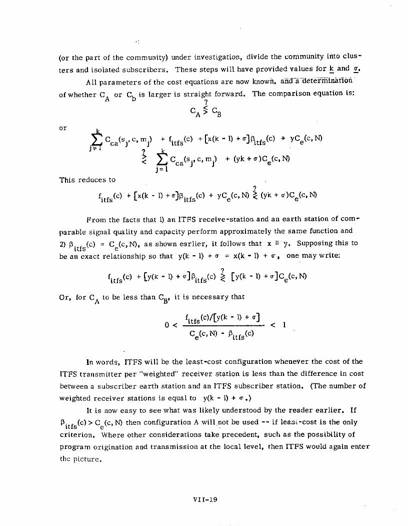
(or the part of the community) under investigation, divide the community into clus-

ters and isolated subscribers. These steps will have provided values for k and a.

All parameters of the cost equations are now known, andaedeterminatiofi

of whether CA or Cb is larger is straight forward. The comparison equation is:

CA CB

or

Cca(sj, c, m) + fitfs(c) + [x(k - 1) + a] tfs(c) + yCe(c, N)

Cca(s, c, m ) + (yk + r)Ce(c, N)j=

This reduces to

fitfs (c) + [x( - 1) + itfs(c) + YCe(c, N) (yk + a)C (c, N)

From the facts that 1) an ITFS receive-station and an earth station of com-

parable signal quality and capacity perform approximately the same function and

2) p itfs(c) = Ce(c, N), as shown earlier, it follows that x : y. Supposing this to

be an exact relationship so that y(k - 1) + a = x(k - 1) + (r, one may write:

fitfs(c) + [y(k - 1) + o] tfs(C) [y(k - 1) + a] Ce(c, N)

Or, for CA to be less than CB, it is necessary that

0 < fitfs(c)/[y(k - 1) + ] <

Ce(c, N) -Pitfs(c)

In words, ITFS will be the least-cost configuration whenever the cost of the

ITFS transmitter per "weighted" receiver station is less than the difference in cost

between a subscriber earth station and an ITFS subscriber station. (The number of

weighted receiver stations is equal to y(k - 1) + a-.)

It is now easy to see what was likely understood by the reader earlier. If

Pitfs(c) > Ce(c, N) then configuration A will not be used -- if leasi-cost is the only

criterion. Where other considerations take precedent, such as the possibility of

program origination and transmission at the local level, then ITFS would again enter

the picture.

VII-19

Another way to look at this comparison is in terms of a likely threshold

value for the weighted number of receive stations. That is, a value of y(k - 1) + o

say [y(k - I) + r]th, such that if, in any particular community the actual value of

y(k - 1) + a does not exceed [y(k - 1) + at h then one may, with certainty, choose

configuration B as the least-cost local subsystem. What are typical values of

[y(k - 1) + 0]th for the cost figures generated in this study? From chapter six,

fitfs(c) = $24, 600 + $61, 600 [c/4]. Thus, with

fitfs (4) = $86, 000

5itfs(4) = $8, 600

and Ce (4, N) = $9, 200 choosing Cw/y = $30, 000

and N= 1,000

then [y(k - 1) + o]th = $86, 000/($9, 200 - $8, 600)

= 130

For a 12-channel subscriber reception system (not very likely),

fitfs (12) = $209, 000

Pitfs(12) = $19, 200

C e(12, N) = $26, 100 choosing Cw/y = $50, 000

and N= 1,000and

[y(k - 1) + o]th = $209, 000/($26, 100 - $19, 200)

= 30

This very large range in threshold value for the number of weighted receive

stations means very simply, that no true threshold exists. That is, each case is

unique. Nevertheless, certainly for any city where y(k - 1) + - is less than about

30, the least-cost local subsystem will use configuration B.

The city of San Jose, California was analyzed with the method presented

above. By actually plotting the locations of all doctors in San Jose on a city map,

it was determined, using an intercluster distance, d, of I and 1/4 miles (corres-

ponds approximately to overhead installation and c = 4), that k = 13 and r = 11.

If l<y<1.25, then 23 < y(k - 1) + o- < 26. For d = 0.4 miles (corresponds

to typical underground cable installation costs and c = 4), k = 22 and ar = 38.

Again, for 1 < y < 1. 25, then 59 < y(k- 1) + v- < 64.

If the 0. 4 mile figure for d is used in the downtown area and the 1. 25 mile

figure used for the residential parts of San Jose, k = 15 and o- = 16. Thus, for

1 < y < 1. 25, 30 < y(k - 1) + - < 33.

VII-20

Can a generalization be made at this point? It seems reasonable to conclude

that ITFS will find only limited application outside of the large metropolitan areas.

With a present population of 445, 709 San Jose is in the lower third of the thirty most

-highly populated urban places. If population alone were an indication of the likely

number of weighted receive stations required in a given city, then certainly fewer

than 50 cities could be expected to select ITFS on a least-cost basis.

Earlier, mention was made of the more general case where the satellite

and local distribution clusters would carry more channels than each subscriber will

receive. This would be needed, for instance, if two professional disciplines were

to share the satellite and, to the extent possible, the local systems. Qualitatively,

the changes that would be required in the above analysis to accommodate this situation

are: 1) The intercluster distance, even though difficult to deal with quantitatively, will

definitely increase. This, of course, is because of the increased cost of a cluster re-

distribution station caused by its increased channel capacity. Ths increased inter-

cluster distance will have a tendency to decrease the number of clusters, k. (Because

the interisolated-subscriber distance would remain the same as before, no significant

change will occur in a-. 2) However, offsetting this will be an increase in _ since

receive stations from which redistribution of the signal will occur must receive c

channels (> ci). 3) fitfs(c) will increase by roughly the same factor as y.

Taken altogether, it appears that these changes will cause the ratio fitfs(c)/

[y(k - 1) + a-] to increase, not decrease. Therefore, the case for ITFS with c > c

seems even less favorable than with c= c..

E. Summary

On a least-cost basis, a satellite system has been shown to be clearly

superior to terrestrial microwave for the transmission of teleconferencing signals

throughout an entire region (several contiguous states). For a smaller area of

coverage, terrestrial microwave will become less expensive as the number of

cities in the teleconferencing network drops well below 100.

Local distribution will probably be accomplished with cable systems. In

any given city, there will in all liklihood be several non-connected cable systems,

the headends of which would be fed directly from their own earth station. Where lo-

cal interconnection of the cable systems is desired, for instance so that local pro-

gramming could occur, an ITFS system should be considered.

VII-21

F. REFERENCES

1. R.D. Swenson, "Investment Costs of Terrestrial Long-Haul Telecom-

munication Facilities", IEEE Trans. on Aerospace and Electronic Systems,

Vol. AES-7, no. 1, pp. 115-121, January, 1971.

2. Comanor and Mitchell, "Cable Television and the Impact of Regulation",

The Bell Journal of Economics and Management Science, 2:154 - 212,

Spring, 1971.

3. Cosgrave and Chipp, "Economic Considerations for Communication Systems",

IEEE Trans. on Comm. Tech., 16:513-525, August, 1968.

VII-22

APPENDIX A

Computer Assisted Instruction (CAI)

Introduction

Computer assisted instruction, along with its sister service, computer

managed instruction, has been widely touted by educators and laymen as a

means for improving education while reducing its costs. It has also been

criticized as dehumanizing and deeply injurious to the total learning

process. Much of the debate on CAI's cost and effectiveness has been

clouded by a lack of understanding of what CAI and CMI really mean.

The purpose of this appendix is to discuss the types of CAI which might

be used in schools, their effectiveness and their costs.

Computers are already playing a major role in many school districts

and private institutions. Accounting and administrative functions are

being handled increasingly by machines. Students use the computer to

solve homework problems. Writers use calculators to produce graphs and

illustrations for their texts. In CAI and CMI, however, the computer

is used to present material to the student directly, measure his progress

and help the teacher select appropriate learning strategies.

Through individualization of material and pace, it ir hoped, CAI

can speed the learning process while reducing learning time. Evidence

for this assertion will be discussed in following sections. Given certain

caveats, there does seem to be justification for optirmism with respect

to CAI performance.

The other advantage of CAI is cost savings. If the cost of hardware

and softwrare can be reduced in the future -- and the trend is definitely

in this direction -- then computers may be able to ease the cost squeeze

which schools are now facing. In the discussion of costs in following

sections, some of the complexities which confuse discussions of cost will

be brought out. Although a general analytical framework will be developed,the only conclusion will be that there is as yet no good estimate of

costs available.

A-i

What are CAI and CMI?

One of the central problems in discussing CAI is that there are

many types of computer assisted instruction. CAI is really a generic.

.. name for a variety of instructional techniques, whose performances vary

widely and whose costs range from ten cents to a thousand dollars per

student instruction hour. Although the diversity of CAI approaches

is somewhat bewildering, it is possible to classify them along several

dimensions for the purpose of further analysis.

In considering CAI, it is easy to fall into the error of the proverbial

blind men who attempted to learn about elephants by examining parts of the

animal. In computer assisted instruction, not even the name CAI is

standard. Other terms meaning approximately the same are CBI (computer

based instruction), CAL (computer augmented learning), and CAE (computer

aided education). In large part, the differences in names reflect only

historical usage by individual groups. For example, CAI was adopted by

IBM for their early systems.1 In part, however, the names were selected

to reflect different philosophies in the use of computers for instruction.

Two issues should be noted somewhat parenthetically. First, CAI

is not identical with programmed instruction (PI), which usually uses

hardcopy texts. In addition, most CAI techniques are more sophisticated

than traditional PI. Second, CMI must always be borne in mind as a substitute

or supplement for CAI. In CMI, a computer is used to help teachers manage

a student's progress through multiple media, such as books, videotapes,

lectures and discussions. Many of the advantages claimed for CAI, in

which material is presented directly by computer, have also been claimed

for CMI.

There seem to be two general philosophies for the use of computers in

instruction. Debate between the two schools has been active and occasionally

bitter. The basic dimension under consideration is whether the student should

control what he is to learn, or whether control should be left in the hands

of teachers or a central instructional program. Much of the debate reflects

a distinction in educational philosophies discussed by Kessen,2 who believed

that extreme forms of the opposing camps in education in general are

A-2

reflected in the writings of Locke and Rousseay. Locke believed that a

child was primarily an unformed person, into which information could be

poured by a teachter. Rousseau considered the child as a whole person,

who would be capable of great gains if left to himself with sufficient

resources. This, of course, is an overstatement of both Locke and

Rousseau, and also of the positions advocated by CAI policy makers.

Nevertheless, the distinction between tutorial and dialog techniques3

reflects the Lockean and Rousseauian positions quite strongly.

Within the basic categories of dialog and tutorial instruction, there

is a wide variation in sophistication, and these ranges w.ll be discussed

in following sections.

The Tutorial Mode

The tutorial mode can be described relatively well along the dimension

of increasing sophistication in basining presentations on prior student

responses.

The most elementary mode of CAI is to use the computer as a Skinnerian

teaching machine. The student is presented a set of sequence of stimuli,

to which he responds. Many PI texts resemble this approach. The first

CAI program, in fact, was created in 1958 by using the computer to simulate

a mechanical teaching machine.

In the next level of sophistication, the student's response to presented

material is used to "branch" him to an appropriate frame, instead of selecting

the frame from a set sequence. This allows a student to move quickly through

material which is easy for him and to receive more instruction in areas

which he is having difficulties mastering. This is basically an online

version of TUDOR-TEXT R type material. The advantages of the computer are

the speed of branching, the potentially greater complexity of the branching,

the ability to provide more levels of difficulty and spread software costs

over more users, and the collection of data for student evaluation and

program improvement.

Within the category of branching programs, there is considerable

diversity. For example, most CAI systems present programs with several

inherently different levels of difficulty, to reflect differences in

A-3

student learning abilities. In addition, the degree of branching within

a given program will vary according to the author's discretion. These

two considerations interact, because greater stratification by levels

of difficulty will reduce the amount of branching required in each.

In the end, it can be said that branching programs vary according

to a hazy dimension which might be called "degree of complexity."

This dimension is important because it profoundly influences programming

costs and because greater complexity allows greater individualization

and prevents the student from "running out of branches" in difficult

areas.

Most systems now in operation depend upon branching logic. The

student's response is usually limited to either a multiple choice

response or a numerical entry. In the next level of sophistication,

branching is done of the basis of unprogrammed responses. In such

systems, the student's response to a question cannot be programmed, but

a "judging routine'"5 is used to determine the appropriate branching. For

example, the student may be asked to work a geometric proof. The computer

program must analyze his progress to check for errors and to judge the

suitability of his approach.

Just as there is a degree of complexity dimension in branching programs,

there is a dimension in unprogrammed response techniques which might be

called "range of judgeable responses." For example, in Albert and Bitzerts

paper, they describe a judging routine for determining whether the figure

a student has drawn is really a triangle. Although this type of routine

is not trivial, it is several orders of magnitude easier than a program

for judging whether a student's approach to evaluating an integral is a

good one. In a program being written as part of a doctoral thesis by

Kimball, 6 the student is given integrals in order to evaluate the "priority

list" he uses in applying evaluation techniques. The program then helps

the student by suggesting different approaches and checking for logical

errors. Such a program would undoubtedly teach the skill of integral

evaluation more thoroughly than a simple branched logic technique, but it

would also be orders of magnitude more expensive to create.

A-4

In the ultimate form of tutorial presentation, termed "Socratic

dialogue," the computer program would use very sophisticated judging

routines (including natural language input), and a vast store of

information and teaching techniques to lead the student through material

by means of a series of questions and unprogrammed responses. This

concept is largely an ideal, but progress is being made in this direction.

For example, the program "ELIZA" has been used at MIT since 1967 to teach

special relativity through Socratic dialog. The program uses natural

language input. Of course, the system is fairly crude; it must often

ask the student to rephrase his response or to ignore the studentts

response and branch arbitrarily. The cost of running even ELIZA

is very large, and the development of natural language processors of

high flexibility will take several years. In time, however, CAI

tutorial techniques should evolve'closer to this ideal.

The Dialogue or Response Mode

The Socratic dialogue approach runs closely to the ideal of the

dialogue mode discussed above. Even in that case, however, the program

is controlling the direction of the learning process. In the dialogue

or response mode, the emphasis is placed on providing the student with

resources to use on his own initiative. Unlike the tutorial mode, the

response mode does not lend itself to discussion along a single dimension.

There are several components of a responding system, and each will be discussed

separately.

Perhaps the most straightforward component is the use of the computer

for computation and display. In this mode, the student would come across

an interesting problem and use the computer to calculate the magnitudes

of certain variables or solve a numerical example. Through the use of

simple languages such as BASIC and flexible display capabilities (including

graphics), such a system could prove useful to students in quantitative

subjects.

An adjunct to this capability is the use of computers for simulation

or gaming. Simulation can be used to give the student a working feeling

for various systems. Through graphic displays, he can see his solution

A-5

of a physics problem acted out, and see the sensitivity of his results

to different variables. Physical and social systems have been modeled

on computers by many organizations as teaching tools. Simulation can

also be used to supplement experiments in the physical sciences. By

eliminating set up time and "settling" delays, simulated experiments

can be run more quickly. Added to laboratory experiences, this technique

can provide more experience in a shorter time.

Another component of responding systems is information retrieval.

Computers can be used in interactive modes to locate information, help

the student search for relevant information and retrieve textual

materials. In a CMI mode, the computer can also route voice or videotape

material to the student. Information retrieval becomes increasingly

important as the student solves more difficult problems. In continuing

professional education, it might easily be the dominant mode of learning.

The final class of components has been termed "responding resources"

by Nelson.9 In responding resources, the student is presented with a

textual or pictorial frame. By a typewritten input or pointing at a

section of the picture with a light pen, the student indicates an interest

he would like to pursue. The computer then provides some explanation of

that section, provides a gaming or simulation exercise, or provides a

motion picture illustration or a process. A "responding resource" is

really a system of the components listed above. The purpose of a responding

resource is simply to provide access to information when a student is inter-

ested in the subject.

In the sections above, a dichotomy was drawn between tutorial and

dialogue modes. In practice, most well thought out systems would include

both aspects. In too many proposals, however, researchers and administrators

appear to be ignorant of this basic distinction and to the fact that there

are levels of complexity within each. Too often, policy makers champion

-or debunk CAI on the basis of limited preconceptions. In doing so, they

act very much like the blind men who argued heatedly about the nature of

elephants.

A-6

Performance

A good deal has been written about the performance of CAI, mostly

from a theoretical viewpoint. Although some hard data is available,

the situation seems far from clear. Rather than try to evaluate

past systems, this section will focus on the issues which must be

considered in the analysis.

First, it should be axiomatic from the preceeding section that

questions on performance must be prefaced by the question, "What type

of CAI is being considered?" General statements are of limited value

in evaluation. Yet many general statements are available on how CAI

should perform. These comments reflect the Locke/Rousseau distinction

made above.

Lockean theorists tend to see CAI systems as uncomplaining tutors

with unlimited patience. CAI appears as a road to uniform high quality

instruction that can be tailored to each student's needs. Suppes (who

is not a strict Lockean) stresses the value of individualization,

listing five areas where individualization can be used: presentation of

material, evaluation or progress, repetition of sections, level of

difficulty, and review. These theorists feel that individualization

will allow each student to learn at his maximum possible rate.

Rousseauian proponents have generally been reelgated to criticst

roles, since most operational CAI experiments have centered around the

tutorial presentation mode. A general warning is summed up by Theodore

Nelson: "CAI in its conventional form enlarges and extends the faults of

the American education system itself." 1 0 Nelson cites tendencies to boredom,

lack of initiative, the tyranny of grades being renewed in terms of number

of frames learned and narrowness of curricula.

Because most measurements of performance have been made in terms of a

Lockean philosophy and have been further confused by the fact that they were

specific to one form of CAI system. The results so far have been mixed but

encouraging. Jamison, et al., were able to demonstratell that CAI could

provide remedial education in mathematics and reading better and more cheaply

than additional classwork. Albert and Bitzer 12 discuss a medical science

A-7

course in which students learned the material in 1/3 to 1/2 the time

of lectures and showed superior retention after 26 weeks. The time

savings of 1/3 has come up in other studies, and while the number is

undoubtedly tied to the level of sophistication of a program, it

is indicative.

Several caveats are in order when discussing the efficacy of CAI.

For example, CMI was used to teach a first-aid course for the American

Red Cross, and improvements on the order of those found in CAI were13

obtained. Since CMI is less expensive in general than CAI, performance/

cost ratios for CAI must be compared to those of CMI as well as to those

of traditional instruction.

In addition, many of the advantages claimed of CAI can also be

claimed of traditional methods. In his insightful review of CAI,

Feldhusen describes a system called BOOK.

All schools at all levels provide for much individualizationof instruction. These activities include reading in BOOK (basicorganization of knowledge)...

"BOOK" is the best medium for individualized instructionso far devised. The student may enter at various places orlevels, proceed at his own rate, branch by his own choice orunder teacher direction, be actively engaged if he does the studyexercises or problems, receive some feedback if the answers aregiven 1 n the back of the book, and be reinforced if he performswell.

In general, it seems fair to say that, even at the multiple choice

branching level, CAI can provide time savings and be cost effective for

some applications. Its performance at more sophisticated tutorial levels

can only be conjectured. In addition, most of the measures used to date

have been unacceptable from the viewpoint of theorists who favor exclusive

or extensive student control of the learning process.

The Cost of CAI

Although the development of evaluated instructional programs has been

a major factor in CAI's slow acceptance in schools, it is generally conceded

that the real stumbling block to adoption is current CAI ts high cost.15

A-8

From the discussion above, the reader understands that it is impossible

to speak of "the" cost of CAI, since different levels of sophistication

in programming will be associated with different financial outlays.

Nevertheless, even fairly simple drill and practice types of programming

are still too expensive to be employed in the bulk of the school system.

The purpose of this section is not to produce a definitive survey

of the costs of various CAI systems. At present, cost data is too

confused and scattered to provide hard numbers. Instead, the various

components of CAI will be discussed, and general considerations

for comparing CAI to traditionally administered instruction (TAI) will

be presented. Although the most useful cost figure is dollars per

student contact hour, it is necessary to discuss component costs first.

Placing costs on a per contact hour basis is a fairly subtle, and

controversial, problem.

Component Costs

CAI costs can be segregated into hardware, software, and operational

costs. Hardware costs can be further subdivided into head-end, communication

and terminal segments. Hardware costs will be considered first.

At the head end, most of the financial investment is tied up in the

central processing unit (CPU), memory banks consisting of tapes and discs,and various peripheral devices such as card readers. In the past, the CPU

mainframe has dominated the investment. With the growth of larger computers,however, which serve many more users, CPU cost per users has fallen rapidly,in comparison to the relatively constant per user investment in memory

and peripherals. In his excellent review of future computer technologies,16

Wallace Riley noted that:

In 1955, for example, of every dollar spent on hardware,20 cents went for peripherals; in 1965, the ratio was more nearly50-50, and by 1975, if not sooner, it will be 80-20 -- the reverseof the 1955 figure.

Much of this growth is due to increased interest in remoteon-line computing, which requires communication channels and amultiplicity of terminal devices. Much of it is also due tothe increased raw power of central processors, which requiremore and fancier peripheral devices to provide them with enoughdata to absorb their output.

A-9

Because of the growing importance of peripherals, costing of CAI

systems must be done with careful attention to the types of input/output

and communication devices needed by the system. Several CAI designers

have made the mistake of extrapolating falling CPU costs directly into

drops in CAI costs. In addition, it is not certain that large CPU's

will be used extensively in CAI systems. Although Socratic dialogue

techniques will require large software systems, most CAI systems can be

handled by local minicomputers, accessing remote data bases. Because of

mass production and comparative simplicity, four or five minicomputers

may cost considerably less than a single CPU of comparable processing power.

Communication costs have been the main focus of this study so they

will not be addressed here. It should be noted, however, that most;

current CAI systems use only local communication lines, although a few

systems (such as the Stanford project) have used long distance communication.

As a result, system designers have tended to ignore communication costs

in the past. As CAI begins to use more advanced techniques, instructional

bases will probably become more clustered, and the importance of long

distance communication should grow accordingly.

Terminal costs are probably the most serious hardware limitation

on CAI's acceptance. At the user's end of the system, there is a model

(modulator-demodulator) to digitize the analog signals passing over the

communication channel, a multiplexer/demultiplexer, if there are several

users at the terminal location, and a display device. Modem and multi-

plexing costs will probably fall dramatically as LSI becomes more prevalent

and the growing demand for time sharing brings them into mass production.

The cost of adequate displays, however, is still very high.

An IBM model 333 teletype costs about $850. Although these displays

are relatively inexpensive, they are very slow and suited only to relatively

simple CAI techniques. A CRT (cathode ray tube) terminal, on the other hand,can display much information rapidly, but is very expensive. For literature

searching, simulation and graphical displays, CRT capabilities are essential.

Unfortunately, image quality is relatively poor on most systems and a

flexible display which allows text editing and other needed functions

costs between $5,000 and $20,000. A fairly simple system, using a

commercial television set and "frame grabber" storage would be inexpensive,

A-10

but communication costs would be exhorbitant. In order to bring down

communication costs, it is necessary for the display to have character

.-- generation and editing capability, both of which are currently very

expensive. Display costs are fairly sensitive to such factors as number

of characters displayed, amount of storage required, editing capabilities

and character generation. The design of a reasonably priced system

requires that the purchaser be familiar with the options available to

him.

The importance of display costs can best be appreciated by the fact

that half of the total per student contact hour costs estimated for the

University of Illinois' proposed PLATO IV system (which includes software,

instructional programming, CPU, memory and communications) arise from

the display terminal. 17 Yet these terminals are projected $1800 devices,

beyond the current state of technology. The reason that displays are so

important in the overall cost picture is that other hardware and software

can be spread over many users. The terminals, however, serve one user

at a time.

Operating system software (excluding instructional programming) is

another expensive factor in system design. It has :been noted that while

"the cost per hardware gate has dropped by two orders of magnitude since

the middle 1950ts, the cost per software instructions has remained just

about constant, at around $10. 18 Rising labor costs in programming

and the growing complexity of large CPU's are probably responsible for

the bulk of this increase. Software creation is especially expensive if

the system will provide the users with several computer languages, different

information bases, and sophisticated accounting procedures.

Operating costs for the head-end system can be large because of

maintenance, operation of the equipment and the management necessary to

run large centers. At the terminal end, there is also a need for maintenance,

and maintenance costs can run close to the yearly depreciation of some

terminals, doubling their effective per/year cost. If the system is to

be used in schools, there will be a need for a center proctor, to maintain

A-11

the equipment, teach use of the system, and keep discipline, if necessary.

Although proctors will be paid less than teachers, their salaries will become

significant if a center has only a half-dozen terminals or so.

The last component to be considered is instructional programming,

which can usefully be subdivided into initial production and revision.

The costs of initial production remain somewhat of a mystery. Published

estimates19,20 seem very crude, and private firms consider such information

to be proprietary. Naturally, the initial cost is dependent upon the level

of sophistication being used in programming strategy. One point of agreement

appears to be that simple programming languages will be needed in the future,

especially if teachers write their own programs. The TUDOR2 1 language

represents the direction in which languages will travel. After a program

is written, it can be modified and updated, with the aid of statistics

gathered from the online users. It is disturbing that estimates of CAI

costs have tended to ignore the costs of updating programs. One of the

principal advantages of using a computer for instruction is the feedback

it can provide to the program designer on the performance of his product.

In the preceeding paragraphs, the author has given qualitative

determinants of system costs. Although some quantitative estimates have

been made,22,23,24 all leave out one or more portions of the preceeding

analysis, and their breakdown of costs on a per student contact hour basis

seems to leave even more to be desired. All three were good efforts,

approaching the problem through different hardware and instructionware

directions. Although all are worth reading, none appears to provide a

complete analysis. Clearly, a great deal more effort is necessary in this

area.

Per Student Contact Hour Costs

Two problems with placing costs on a per student contact hour basis

are annualizing the costs and placing them on a per hour basis. The first

is logically prior to the second, and also somewhat more straightforward.

Annual costs consist of amortizing capital costs and computing

operating costs. As noted above, operating costs consist of maintenance,supervision, communications, and the operation of equipment. Major

capital costs consist of hardware, software, and instructional programming.

A-12

To annualize hardware depreciation, it is necessary to know the equipment's

lifetime in years (n), the cost of capital for the user (i), and the initial

cost of the equipment, (Co). The annual cost (Ca) for each piece of

equipment is then given by:

CC =

j=1

The equipmentts lifetime in years may be either its physical lifetime,

or the time span over which it is not made obsolete by newer equipment.

Leasing the equipment, rather than buying it, may be the best choice,

especially if the user does not wish to maintain it himself, cannot use the

capital equipment tax writeoff or feels that the equipment should soon be

replaced by more modern devices. Previous estimates of system costs have

tended to use straight line depreciation, which can be a poor estimate

if the cost of capital is high, as it might be for a hospital or individual

professional.

Software should also be amortized over time. As each piece of software

is written, it should be capitalized, and its useful life estimated. If it

is purchased from another system, this becomes its initial cost. Because

identical hardware systems can use identical software, if there is

cooperation between users, and because the cost of producing software is

high, computer systems for CAI will benefit greatly if they exchange

software or jointly pay for software design. The lifetime of software is

difficult to estimate, and is determined almost exclusively by

obsolescence. It is a matter of judgement whether major revisions are

capitalized or treated as annual costs.

Instructional programming, like system software, benefits from

cooperative production and use. If each. teacher writes his own program,even using a simple language, instructional progeamming costs will be high.

At the other extreme, if programs are produced nationally, their cost per

user will become negligible (in larger fields). Socratic dialogue and other

sophisticated techniques will probably require national origination. For

A-13

less advanced techniques, programs will probably be produced by individuals

and sold competitively, much as textbooks are now. Also like textbooks,

programs probably will be developed only in larger fields, with live

lectures being used in small growing fields. One way to get around the

"big brother" connotation of national origination would be to produce

programs modularly, and let the teacher build programs (with the aid

of the computer). Another approach to localizing instruction is

illustrated by Kimball' s calculus tutor, in which the teacherts

personal. approaches and priorities in problem solving can be learned by

the program and used as the basis for instruction of the students. Whatever

approach is used to create programming, the advantages of cooperative usage

should be realized and mechanisms should be provided for the feedback

necessary in the revision of programs.

Once costs are annualized, it is necessary to place them on a per

student contact hour basis. In a sense, this step has already been done

for instructional programming. Once the number of students using the system

per year is known, and the system lifetime is estimated. the per contact

hour cost falls out immediately.

The cost of the CPU and head end software are determined by system

utilization. Ideally, the system would be used 100%, 100% of the time.

In practice, this is impossible and a false goal. It is impossible, because

usage will vary with time of day, and because systems must be designed

to accomodate growth in the number of users. The peak-to-average consideration

can be alleviated somewhat by a tarrif structure that encourages users to

use the system during off peak hours. To simply legislate that the system

will be used evenly, however, would make it unattractive from the userst

standpoint, and it would probably not be adopted. A 50% utilization rate

of the CPU is considered almost extraordinaty for the most current systems.

The problem of growth can be somewhat alleviated by designing the system

to be able to grow by adding modular components, but this cannot always be

done. Attention should be paid, however, to the comparative economics of

modular growth versus major additions.

A-14

Alpert and Bitzer ts cost estimates for PLATO IV illustrate just how26

important utilization really is to system efficiency. Alpert and Bitzer

project a per student contact hour cost of about $0.60 (including hardware

and instruction ware) which would be competitive with current educational

costs in schools. However, they assume 100% utilization of the CPU and

student terminals. In addition, they assume that the system would be used

k~ weeks per year, 44 hours per week, or 2000 hours per year. The regular

school year, in contrast, is only 1050 (6 hours per day, 35 weeks per year).

In another paper27 the author recalculates the per student contact hour cost,

using 60% CPU utilization, 60% terminal utilization, and a 1575 hour school

year (allowing for night usage by adults and a slightly longer school day).

The costs jumped by a factor of two, and were no longer attractive for

school use.

On the college level, and in the military, longer student days could

be used, bringing the effective system usage to something near 2000 hours

per day. Problems of CPU utilization would still remain. In addition, the

traditional costs of college and specialized instruction are much higher

than they are on the elementary school level. It can be expected, then,

that the first use of CAI may be on the college level. In fact, Florida

State University offers a freshman physics course by CAI.

For professionals, high utilization rates for the terminals are impractical.

Although some of the terminal costs may be taken by using the terminal for

other computational functions, it is doubtful that professionals would

adopt a system for which they had to wait in line for any length of time.

Moreover, it would be best to bring terminals into professionalst offices,

which would almost certainly mean low utilization rates. Although the problem

should be eased as the cost of displays, modems and multiplexers decline,

it appears that CAI will not be attractive for professionals in the near

future unless teletype terminals are used. This in turn limits the sophistication

possible in programming and will make literature searching tedious and slow,

casting doubt on system acceptability.

A-15

CAI vs. TAI

In a sense, comparing CAI to TAI is like comparing apples and oranges.

Traditionally administered instruction is labor intensive, and ideally

suited to short school days. CAI is hardware intensive, and therefore

sensitive to utilization rates. In addition, instructional programming

must be spread over many users, whereas live class instruction can be

done effectively by individual teachers. In constraining CAI to normal

school days and lock-step progress through grades, a distorted unfavorable

view is presented of its economics. One of the main characteristics of

CAI is its ability to teach material faster. Randall and Blashke

calculated that if students were allowed to progress through grades

faster as a result of CAI, the number of years saved would make CAI look

competitive with traditional costs. For the school system, the issues

of teacher replacement, length of the school day and progress through

grades are explosive issues, subject to considerable inertia and resistance --

much of it justified.

In less traditional areas, like vocational education, continuing

professional education and, to some extent, the college system, the time

savings of CAI could prove decisive. If a professional could learn without

travelling to school and pick up competencies rapidly, the amount of time

saved by his company might justify CAI costs in the range which producers

now claim they can reach.

Conclusion

The reader will probably find the absence of hard cost figures dis-

conserting, especially in light of the communication costs derived in

technical sections of this report. This discomfort is certainly justified,since communication costs cannot be used meaningfully until other system

costs are known. Unfortunately, the area of CAI has proven to be particularly

difficult to quantify. Studies references above, which attempted to determine

CAI costs, all had methodological weaknesses, or used assumptions which do

not seem reasonable or desirable. Moreover, many of the costs seem to be

"off the top of the head" estimates, of doubtful value. In general, it

seems that CAI costs for current systems range between $1 to $10 per hour

A-16

of student contact. The lower estimate is near the cost of textbooks

in college and about double the total cost in elementary and secondary

schools. As component prices continue to fall and software becomes,

available, the economic outlook for CAI should continue to improve.

It is doubtful, however, whether educators or private groups will be

willing to make major investments until instructionware packages are

improved considerably and cost estimates become more reliable.

A-17

References

1. Zinn, Karl L. and McClintock, Susan, A Guide to the Literature onInteractive Use of Computers for Instruction, Second Edition,Series One Paper, ERIC Clearinghouses on Media and Technology,January 1970, p. 2.

2. Kessen, William, The Child, Wiley, New York, 1965.

3. Suppes, Patrick, "The Uses of Computers in Education," ScientificAmerican, September 1966, (pp. 207-220), p. 219.

4. Rath, Gustave J., "The Development of Computer-Assisted Instruction,"IEEE Transactions on Human Factors in Electronics, Vol. HFE-8,No. 2, June 1967, (pp. 60-63), p. 61.

5. Alpert, D. and Bitzer, D. L., "Advances in Computer-Based Education,"Science, 167, 20 March 1970, (pp. 1582-1590), p. 1984.

6. Kimball, Ralph B., Department of Electrical Engineering, StanfordUniversity, Stanford, California, private discussions withauthor.

7- Suppes, Op. Cit., p. 219.

8. Schwartz, Guenter, Kromhout, Ora M. and Edwards, Steve, "Computers inPhysics Instruction," Physics Today, September 1969, (pp. 41-49),pp. 41-42.

9. Nelson, Theodor, H., "No More Teachers' Dirty Looks," Computer Decisions,September 1970, (pp. 16-23), p. 20.

10. Nelson, Op. Cit., p. 19.

11. Jamison, Dean, Fletcher, J. Dexter, Suppes, Patrick and Atkinson, Richard,Cost and Performance of Computer-Assisted Instruction for Educationof Disadvantaged Children, Conference on Education as an Industry,4-5 June, 1971, sponsored by Universities-National Bureau Committeefor Economic Research, 261 Madison Avenue, New York, 10016.

12. Alpert and Bitzer, Op. Cit., p. 1585.

13. Flanagan, John C., "How Instructional Systems Will Manage Learning,"Nation's Schools, 86, 4 October 1970 (pp. 65-69, 120), p. 67.

14. Feldhunsen, John H., A Position Paper on CAI Research and Development,A Series Two Paper, ERIC Clearinghouses on Media and Technology,February 1970, p. 2.

15. Wolff, Howard, "CAI Edges Slowly into the Classroom," Electronics,August 5, 1968 (pp. 163-168), p. 163.

A-18

References (continued)

16. Riley, Wallace B., "Wanted for the 170's: Easier-to-Program Co'ters,"Electronics, September 13, 1971 (pp. 61-84), p. 77.

17. Alpert and Bitzer, Op. Cit., p. 1589.

18. Riley, Op. Cit., p. 62.

19. Kopstein, Felix F., and Seidel, Robert J., "Computer-Assisted InstructionVersus Traditionally Administered Instruction: Economics," Audio-Visual Communication Review, 16, 2, Summer 1968, (pp. 147-175--, pp. 148 ff.

20. Alpert and Bitzer, Op. Cit., p. 1587.

21. Ibid.

22. Jamison, et al., Op. Cit.

23. Alpert and Bitzer, Op. Cit.

24. Kopstein and Seidel, Op. Cit.

25. Kimball, Ralph R., see reference 6.

26. Alpert and Bitzer, Op. Cit., p. 1587.

27. Panko, Ra3y, A Review of the Probable Costs of PLATO IV., Center forRadar Astronomy, Durand Building, Stanford University, Stanford,California 94305, August 12, 1971.

28. Randall, Ronald and Blaschke, Charles, "Educational Technology;Economics, Management, and Public Policy," Educational Technology, 1 ,June 30, 1968, (pp. 5-13), p. 7-

A-19

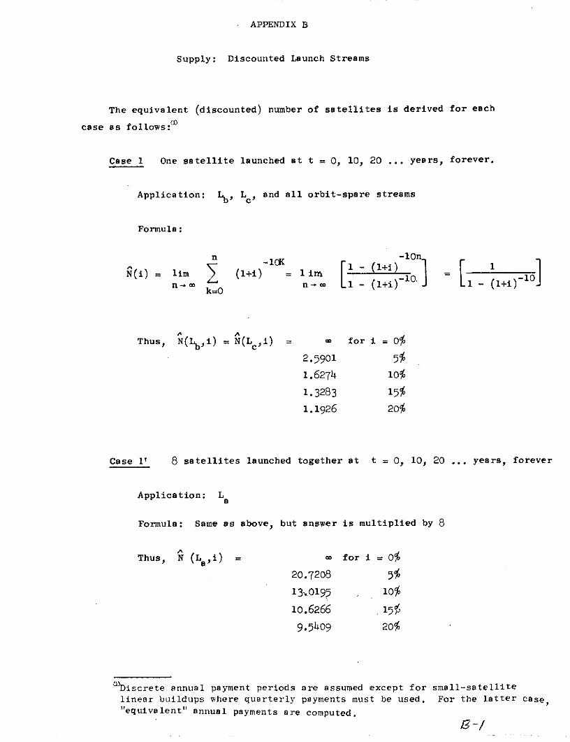
APPENDIX B

Supply: Discounted Launch Streams

The equivalent (discounted) number of satellites is derived for each

case as follows:W

Case 1 One satellite launched at t = 0, 10, 20 ... years, forever.

Application: Lb, Lc, and all orbit-spare streams

Formula:

n -10n_

N(i) = lim (1+i) = 1 irn 10. -10n-m n - (l+i) 1 - (+

k=0

Thus, N(Lbi) N(L Ci) = 0 for i = 0%

2.5901 5%

1.6274 10%

1.3283 15%

1.1926 20%

Case 1' 8 satellites launched together at t = 0, 10, 20 ... years, forever

Application: La

Formula: Same as above, but answer is multiplied by 8

Thus, N (L ,i) for i = 0%

20.7208 5%

13~0195 . 0%

10.6266 15%

9.5409 20%

ODiscrete annual payment periods are assumed except for small-satellite

linear buildups where quarterly payments must be used. For the latter case,"equivalent" annual payments are computed.

Case 2 One satellite launched at t-= 0, and every 1 years thereafter,

forever

Application: Ld

Formula: N(i) = lim (1 + 1/4) =1n o k=O - ( + i/4)-5

Thus, N(Ld, i) = for i = 0%

16.6052 5%

8.6096 10%

5.9481 15%

4.6195 20%

Case 3 Infinite launch chains (one satellite every 10 years):

one chain initiated each at t = O, 10, 20 ... years, forever.

Application: Lf

A2

Formula: N(i) = (Case 1, i)] 2 1 - (+ -10

Thus, N(Lf, i) = for i = 0%

6.70o86 5%2.6486 10%

1.7645 15%

1.4223 20%

1Case 4 Infinite launch chains (one satellite every 1 years): one chain

initiated each at t = 0, 10, 20 ... years, forever.

B-2

Application: L

Formula: N(i) = N(Case 2, i) * N(Case 1, i)

Thus, N(Le i) = for i = 0%

43.0091 5%

14.o116 10%

7.9010 15%

5.5093 20%

B-3

APPENDIX C

Demand: Discounted Sold Capacity

C

The equivalent (discounted) total capacity sold depends upon demand

functions and the interest rate as follows:

Case D1 Constant demand

Application: D 1is Db , Dl c

Formula:

o (20 W for i = 5%-it 1 i 10 W 10%W(Dl, i) = W e - t dt = 6.666w 15

o 5 W 20%

Thus, i W(Dla, i) W(Dlb, i) W(Dlc , i)

5% 14,080 13,440 1,760

10% 7,04 6,720 880.0

15% 4,693 4,480 586.720% 3,520 3,360 440.0

0) Continuous lease payments are assumdd. Satellite capacity may attimes exceed demand, but we presume it cannot be sold. Since some ofour posited demand functions grow continuously, continuous discounting(exponential) will be used. This is not unrealistic: several proposedsatellite owners (e.g. COMSAT) expect to lease their transponders on amonthly basis.2 This is a tantamount to continuous leasing.

C-1

Case D Linear demand, 0Ot<10 years; constant demand thereafter.

Application: D2d , D2b

Formula:

1 te- i dt + -it dtW(D2, 1) = W -t d

o 10

e 10 15.739 w for i = 5%w 10 6.3212 W 10

10 i 3.528 w 15%

2.1617 W 20%

A

Thus, i W(D 2 d, i) W(D 2 b' i)

5% 11,080 10,577

10% 4,450 4,248

15% 2,431 2,320

20% 1,522 1,453

Case D3 Linear demand, Ol0t<

Application: D3e , D3

Formula:

r (0 W for i = 5%)te -'it =I

W(D3, i) = W - t dt = W 1%

o 1014.444 W 15%

2.5 W 20%

C-2

Thus, i W(D3ei) W (D3f i)

5% 28,160 26,880

10% 7,040 6,720

15% 3,129 2,987

20% 1,760 i, 683o

C-3

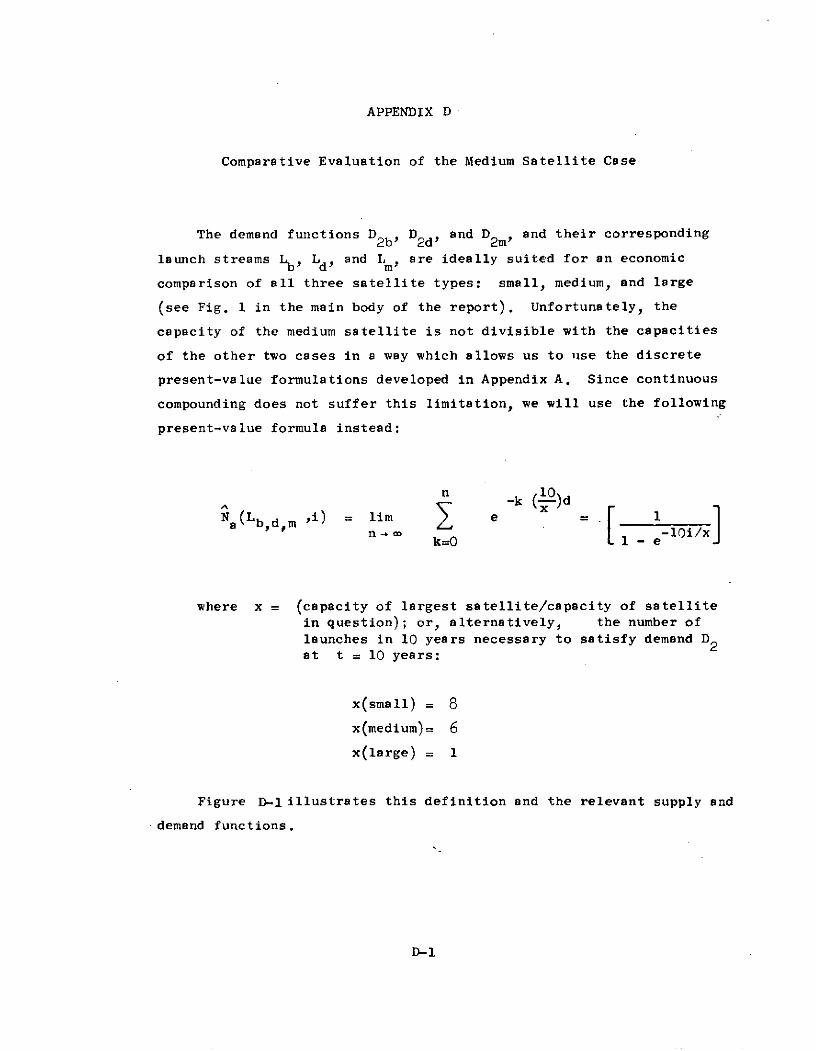
APPENDIX D

Comparative Evaluation of the Medium Satellite Case

The demand functions D2b , D2d) and D2m , and their corresponding

launch streams Lb, Ld, and L , are ideally suited for an economic

comparison of all three satellite types: small, medium, and large

(see Fig. 1 in the main body of the report). Unfortunately, the

capacity of the medium satellite is not divisible with the capacities

of the other two cases in a way which allows us to use the discrete

present-value formulations developed in Appendix A. Since continuous

compounding does not suffer this limitation, we will use the following

present-value formula instead:

n 10n -k (-)dNa(Lb,dm ,i) Lim e -k ( = 1

n k=O 1 - e i/x

where x = (capacity of largest satellite/capacity of satellite

in question); or, alternatively, the number of

launches in 10 years necessary to satisfy demand D2at t = 10 years:

x(small) = 8

x(medium)= 6

x(large) = 1

Figure D-1 illustrates this definition and the relevant supply and

.demand functions.

D-1

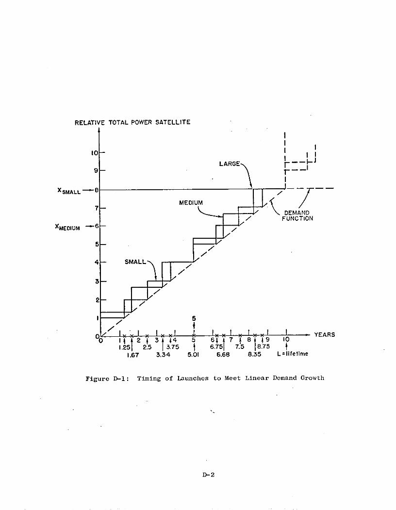
RELATIVE TOTAL POWER SATELLITE

10 I

LARGE F -9-

XSMALL --- 8 MEDIUM =../ FUNCTION

XMEDIUM -6

5-

4- SMALL

0C I : x X YEARS0 4 3 4 5 6 7 8 10

1.251 2.5 1 3.75 6.751 7.5 8.75 f1.67 3.34 5.01 6.68 8.35 L=IIfetime

Figure D-l: Timing of Launches to Meet Linear Demand Growth

D- 2

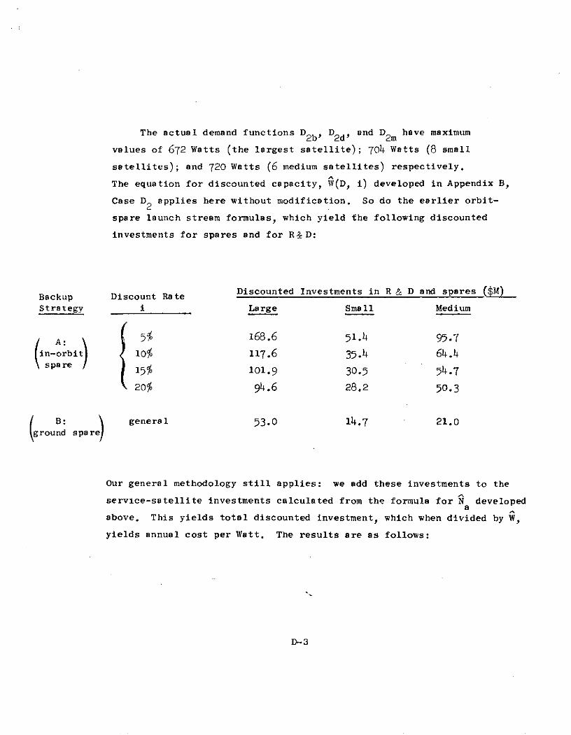
The actual demand functions D2b, D2d , and D2m have maximum

values of 672 Watts (the largest satellite); 704 Watts (8 small

satellites); and 720 Watts (6 medium satellites) respectively.

The equation for discounted capacity, W(D, i) developed in Appendix B,

Case D2 applies here without modification. So do the earlier orbit-

spare launch stream formulas, which yield the following discounted

investments for spares and for R& D:

Backup Discount Rate Discounted Investments in R & D and spares ($M)

Strategy i Large Small Medium

A: 5% 168.6 51.4 95.7

in-orbi 10% 117.6 35.4 64.4spare t 15% 101.9 30.5 54.7

20% 94.6 28.2 50.3

gouB: spare) general 53.0 14.7 21.0

Our general methodology still applies: we add these investments to the

service-satellite investments calculated from the formula for Na developed

above. This yields total discounted investment, which when divided by W,

yields annual cost per Watt. The results are as follows:

D-3

Discount Rate Discounted Supplied and Demanded Capacity

.1 Supply, N Demand, W

Large Small Medium Large Small Medium

5% 2.541 16.529 12.500 10,577 11,080 11,320

10% 1.582 8.511 6.534 4,248 4,450 4,550

15% 1.287 5.862 4.521 2,320 2,431 2,485

20% 1.156 4.521 3.531 1,453 1,522 1,558

Figure D-2 summarizes the results for investment and annual cost per Watt.

Results for the small and large satellites are virtually identical to those

obtained for cases 4 and 5 respectively ( see Fig. 3 in the main report). The

slightly lower ( < 3 % ) values obtained here differ slightly because of the con-

tinuous discounting formula used. Hence the same conclusions apply: for the

orbit-spare strategy, the small satellite is the better choice for i> 6%; for

the ground-spare strategy, the large satellite is the better choice for i<l%.

As expected, the medium satellite is the most expensive choice.a

Results are actually biased over 7% in favor of the medium case (i.e., bythe ratio of 720 Watts/672 Watts). Without this bias, the medium satellitewould have the highest annual cost per Watt, even at i= 20%.

D-4

WATTS MEDIUM

720..-- 1. SMALL704--672 - - LARGE

D2'

"~ 600 -.9 M10 YEARS

S MEDIUM 0 Annual Cost per WattE c

*P.. VS.500- 00100- MEDIUM

Present Value of Invest- Discount Ratement /

H\ vs.U 400 Discount Rate H 80

O 300- a 60

2 0 0 - - 40

) LARGE zU) z

i. 100 - --- }SMALL 20 l

-LARGE

S 5 10 15 20 0 5 10 15 20DISCOUNT RATE (%)- DISCOUNT RATE (%)-

- In-orbit spare---- ground spore

Figure D-2: Summary of Results for Investment and Annual Cost Per Watt

D-5

APPENDIX E

The Number Of Cities In The Rocky Mountain Region In Three

Size Categories*

Total Region

all cities 1168

greater than 2, 000 361

greater than 5, 000 189

greater than 10, 000 100

/ greater greater greaterState all cities than 2, 000 than 5, 000 than 10, 000

Arizona / 87 59 29 13

Colorado , 278. 72 42 26

Idaho / 200 41 14 9

Montana 135 38 17 8

Nevada 32 21 14 9

New Mexico 105 46 26, 15

Utah 227 60 36 ' 15

Wyoming 94 24 11 5

* U.S. Bureau of the Census, U.S. Census of Population. 1970 -- umber OfInhabitants, Final Report PC(1)-A4, A7, A14, A28, A30, A33, A , and A52.

E-1