n-gram modeling of tabla sequences using variable - smartech
TRANSCRIPT

N-GRAM MODELING OF TABLA SEQUENCES USINGVARIABLE-LENGTH HIDDEN MARKOV MODELS FOR
IMPROVISATION AND COMPOSITION
A ThesisPresented to
The Academic Faculty
by
Avinash Sastry
In Partial Fulfillmentof the Requirements for the Degree
Master of Science inMusic Technology
Georgia Tech Center for Music TechnologyGeorgia Institute of Technology
December 2011

N-GRAM MODELING OF TABLA SEQUENCES USINGVARIABLE-LENGTH HIDDEN MARKOV MODELS FOR
IMPROVISATION AND COMPOSITION
Approved by:
Dr. Gil Weinberg, AdvisorGeorgia Tech Center for Music TechnologyGeorgia Institute of Technology
Professor Jason FreemanGeorgia Tech Center for Music TechnologyGeorgia Institute of Technology
Dr. Rebecca FiebrinkDepartment of Computer SciencePrinceton University
Date Approved: 15 September 2011

To Appa and Amma,
for everything that they’ve done for me
iii
ACKNOWLEDGEMENTS
I am deeply indebted to Dr. Parag Chordia, without whose guidance this thesis
would not be here today. I would also like to thank Dr. Gil Weinberg and Prof.
Jason Freeman for their invaluable comments and their feedback throughout the
entire process. I’m extremely grateful to Dr. Rebecca Fiebrink, from the the Dept. of
Computer Science at Princeton University for sparing the time and effort to review the
thesis on very short notice. Also, I would be nowhere, assuming I am somewhere right
now, without the contributions of my colleagues Trishul Mallikarjuna, Aaron Albin
and Sertan Senturk to this project. I would like to thank Trishul for laying down
the basic architecture of the Prediction Suffix Tree, parts of which are still being
used intact within the framework. Aaron’s help in researching and designing the
smoothing algorithms for the project is greatly appreciated, and Sertan’s MATLAB
code for audio segmentation and feature extraction ensured that the project could be
completed in time. I would also like to thank Alex Rae, whose tabla sequencer proved
to be very handy in creating the audio database. Finally, I would like to express my
gratitude towards my family, all my friends, and my colleagues at the GTCMT for
their undying moral support over the last two years. This project is supported by
the National Science Foundation under NSF grant no. 0855758.
iv

TABLE OF CONTENTS
DEDICATION . . . . . . . . . . . . . . . . . . . . . . . . . . . . . . . . . . iii
ACKNOWLEDGEMENTS . . . . . . . . . . . . . . . . . . . . . . . . . . iv
LIST OF TABLES . . . . . . . . . . . . . . . . . . . . . . . . . . . . . . . vii
LIST OF FIGURES . . . . . . . . . . . . . . . . . . . . . . . . . . . . . . viii
SUMMARY . . . . . . . . . . . . . . . . . . . . . . . . . . . . . . . . . . . . ix
I INTRODUCTION . . . . . . . . . . . . . . . . . . . . . . . . . . . . . 1
1.1 Motivation . . . . . . . . . . . . . . . . . . . . . . . . . . . . . . . . 5
1.2 Hypothesis . . . . . . . . . . . . . . . . . . . . . . . . . . . . . . . . 6
1.3 Contribution . . . . . . . . . . . . . . . . . . . . . . . . . . . . . . . 7
II BACKGROUND AND RELATED WORK . . . . . . . . . . . . . 10
2.1 Creativity and Computation . . . . . . . . . . . . . . . . . . . . . . 10
2.2 Generative Music . . . . . . . . . . . . . . . . . . . . . . . . . . . . 13
2.3 Tabla . . . . . . . . . . . . . . . . . . . . . . . . . . . . . . . . . . . 16
2.3.1 Why the tabla? . . . . . . . . . . . . . . . . . . . . . . . . . 18
III CONCEPTS . . . . . . . . . . . . . . . . . . . . . . . . . . . . . . . . . 22
3.1 N-Gram Modeling . . . . . . . . . . . . . . . . . . . . . . . . . . . . 22
3.2 Markov Models . . . . . . . . . . . . . . . . . . . . . . . . . . . . . 24
3.3 Prediction Suffix Trees . . . . . . . . . . . . . . . . . . . . . . . . . 27
3.3.1 The Zero Frequency Problem . . . . . . . . . . . . . . . . . . 29
3.3.2 Smoothing . . . . . . . . . . . . . . . . . . . . . . . . . . . . 30
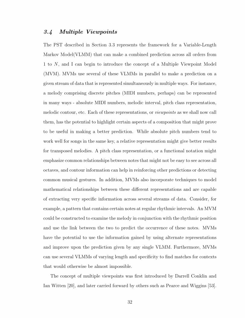
3.4 Multiple Viewpoints . . . . . . . . . . . . . . . . . . . . . . . . . . . 32
3.4.1 Entropy . . . . . . . . . . . . . . . . . . . . . . . . . . . . . 33
3.4.2 Merging Viewpoints . . . . . . . . . . . . . . . . . . . . . . . 35
3.4.3 Perplexity . . . . . . . . . . . . . . . . . . . . . . . . . . . . 36
v

IV VLMM IMPLEMENTATION . . . . . . . . . . . . . . . . . . . . . . 37
4.1 **bol Database . . . . . . . . . . . . . . . . . . . . . . . . . . . . . 37
4.2 VLMM . . . . . . . . . . . . . . . . . . . . . . . . . . . . . . . . . . 38
4.2.1 Viewpoints . . . . . . . . . . . . . . . . . . . . . . . . . . . . 38
4.2.2 Prediction Scheme . . . . . . . . . . . . . . . . . . . . . . . . 39
4.2.3 Merging Predictions . . . . . . . . . . . . . . . . . . . . . . . 46
4.3 Evaluation . . . . . . . . . . . . . . . . . . . . . . . . . . . . . . . . 47
4.4 Results . . . . . . . . . . . . . . . . . . . . . . . . . . . . . . . . . . 48
V VLHMM IMPLEMENTATION . . . . . . . . . . . . . . . . . . . . . 54
5.1 Hidden Markov Models . . . . . . . . . . . . . . . . . . . . . . . . . 54
5.2 Database . . . . . . . . . . . . . . . . . . . . . . . . . . . . . . . . . 56
5.3 VLHMM . . . . . . . . . . . . . . . . . . . . . . . . . . . . . . . . . 58
5.3.1 Training . . . . . . . . . . . . . . . . . . . . . . . . . . . . . 59
5.3.2 Prediction Scheme . . . . . . . . . . . . . . . . . . . . . . . . 59
5.3.3 Evaluation . . . . . . . . . . . . . . . . . . . . . . . . . . . . 61
5.4 Results and Discussion . . . . . . . . . . . . . . . . . . . . . . . . . 62
VI FUTURE WORK . . . . . . . . . . . . . . . . . . . . . . . . . . . . . 68
VII CONCLUSION . . . . . . . . . . . . . . . . . . . . . . . . . . . . . . . 70
REFERENCES . . . . . . . . . . . . . . . . . . . . . . . . . . . . . . . . . . 72
vi

LIST OF TABLES
1 Tabla strokes used in the current work. The drum used is indicated,along with basic timbral information. “Ringing” strokes are resonantand pitched; “modulated pitch” means that the pitch of the strokeis altered by palm pressure on the drum; “closed” strokes are short,sharp, and unpitched. . . . . . . . . . . . . . . . . . . . . . . . . . . . 19
2 Histogram showing the list of all possible bi-grams and their counts ina sequence S = {ABAACAABAA}. . . . . . . . . . . . . . . . . . . 23
3 Histogram showing the counts for all possible bi-grams for the sequenceS = {RSSRRSSRRSS}. . . . . . . . . . . . . . . . . . . . . . . . . 25
4 Transition matrix of a first-order Markov model built on the sequenceS = {RSSRRSSRRSS}. . . . . . . . . . . . . . . . . . . . . . . . . 25
5 Snippet of a typical **bol file. . . . . . . . . . . . . . . . . . . . . . . 38
6 Table summarizing the four viewpoints used in the VLMM system. . 39
7 Average and median of perplexity results for for back-off, 1/N, andparametric (with exponent coefficient equal to 1) smoothing methods.Results for combined models using a maximum order of 10. MV refersto the multiple-viewpoints model in which the SxD and SxPIC view-points have been incorporated. . . . . . . . . . . . . . . . . . . . . . . 51
8 Summary of perplexity results for LTM for order 10. . . . . . . . . . 51
9 Table showing the change in perplexity with increasing order of theVLHMM . . . . . . . . . . . . . . . . . . . . . . . . . . . . . . . . . . 62
10 Average perplexity for each test song, and the median perplexity acrossall test songs for each order. . . . . . . . . . . . . . . . . . . . . . . . 63
11 Table showing the average perplexity by composition type . . . . . . 65
12 Table showing the average computation time per stroke in seconds forVLHMMs of orders 1, 2, 3 . . . . . . . . . . . . . . . . . . . . . . . . 66
vii

LIST OF FIGURES
1 A picture showing the two drums of the tabla. The one on the left iscalled bayan, and it is used to produce resonant bass tones. The drumon the right is the dayan, capable of producing sharp clicks and ringingtones. . . . . . . . . . . . . . . . . . . . . . . . . . . . . . . . . . . . 16
2 A simple first-order Markov model built on observed weather condi-tions on a daily basis [39]. The figure shows two states for the weatheron a given day, rainy(R) and sunny(S). The arrows represent the tran-sition from one state to the next. . . . . . . . . . . . . . . . . . . . . 25
3 Diagram showing a PST trained on the sequence S = {ABAC}. Thetop level represents independent symbols ’A’, ’B’, ’C’. The childrenrepresent bi-grams that start with the parent, and their children rep-resent tri-grams and so on. The cirle on the top right of every node isthe number of times that a node has been seen so far, and the circleto the bottom right shows its probability. . . . . . . . . . . . . . . . . 28
4 Sketch showing the relationship between the probabilities in a finitedistribution (the yellow lines) and the entropy of the distribution (rep-resented by the red lines). The distribution on the left has a lowerentropy because it has one clear prediction. . . . . . . . . . . . . . . . 35
5 Figure showing an overview of the prediction scheme used in the VLMM. 40
6 Figure showing the family of curves represented by the Parametricsmoothing scheme. . . . . . . . . . . . . . . . . . . . . . . . . . . . . 45
7 Entropy of predictions plotted against increasing model order . . . . . 49
8 Comparison of perplexity between BO and 1/N models. . . . . . . . . 52
9 Perplexity as a function of exponent coefficient in parametric model.There seems to be an optimal range between 1 and 2. . . . . . . . . . 53
10 Histogram showing range of perplexity values when predicting strokesfor the Back-Off model . . . . . . . . . . . . . . . . . . . . . . . . . . 53
11 An example of a simple Hidden Markov Model with 2 hidden states(Rainy,Sunny) and 3 visible symbols(Walk, Shop, Clean). . . . . . . . . . . . 55
12 Comparison between number of nodes in the PST at a given level vs.the theoretical maximum . . . . . . . . . . . . . . . . . . . . . . . . . 61
13 Figure describing the cross-validation scheme used for the VLHMMsystem . . . . . . . . . . . . . . . . . . . . . . . . . . . . . . . . . . . 67
viii

SUMMARY
This work presents a novel approach for the design of a predictive model of mu-
sic that can be used to analyze and generate musical material that is highly context
dependent. The system is based on an approach known as n-gram modeling, often
used in language processing and speech recognition algorithms, implemented initially
upon a framework of Variable-Length Markov Models (VLMMs) and then extended
to Variable-Length Hidden Markov Models (VLHMMs). The system brings together
various principles like escape probabilities, smoothing schemes and uses multiple rep-
resentations of the data stream to construct a multiple viewpoints system that enables
it to draw complex relationships between the different input n-grams, and use this in-
formation to provide a stronger prediction scheme. It is implemented as a MAX/MSP
external in C++ and is intended to be a predictive framework that can be used to
create generative music systems and educational and compositional tools for music. A
formal quantitative evaluation scheme based on entropy of the predictions is used to
evaluate the model in sequence prediction tasks on a database of tabla compositions.
The results show good model performance for both the VLMM and the VLHMM
while highlighting the expensive computational cost of higher-order VLHMMs.
ix

CHAPTER I
INTRODUCTION
The work presented here describes a context dependent predictive system for model-
ing rhythmic sequences from a set of tabla compositions. Its main task is to extract
information from audio or symbols, use this information to build a database of mu-
sical sequences, and make predictions on possible continuations for a given sequence.
To achieve this, it draws upon concepts from various fields - n-gram modeling and
Markov models from Natural Language Processing(NLP), the concepts of entropy and
smoothing from information theory, and Variable-Length Hidden Markov Models, or
VLHMMs from speech processing. These concepts are built into a unified framework
known as a multiple viewpoints system. Such a system makes use of multiple repre-
sentations of the data to model and represent complex relationships between different
streams of information, and uses a merging schema to combine this information into
a single prediction for the next event. The result is a versatile model that is capable
of using information across all orders of the model, providing very specific matches
for sequences found within the database, and falling back on general lower-order pre-
dictions if it unable to find suitable matches. The system is evaluated on two fronts
- a symbolic library and a synthesized audio database of tabla compositions. Note
that it is not intended to be a generative work, but a predictive framework that can
be used to implement generative systems and educational software.
The tabla is one of the main percussive instruments used in traditional North-
Indian classical music (NICM). It consists of two drums capable of producing a wide
range of timbres, from short clicks to sustained bass tones. Music on the tabla is
generally rhythmic in nature, consisting of patterns constructed by the juxtaposition
1

of sounds of different timbres. Each of these sounds is produced by striking specific
parts of the drum membranes. Tabla players make use of basic principles of rhyth-
mic and timbral organization along with sophisticated techniques of composition and
improvisation to create complex progressions of events. This is discussed in much
greater detail in Section 2.3.
The project consists of two parts. The first is a system based on Variable-Length
Markov Models (VLMMs) that is designed to work on symbolic notation. The second
part extends this concept to audio data, using Variable-Length Hidden Markov Mod-
els(VLHMMs) instead of VLMMs, however the underlying processes for both parts
are strongly related. Both systems make use of an ensemble of prediction models
- a set of VLMMs or VLHMMs working together on different streams of data - to
construct a set of Prediction Suffix Trees (PSTs). Each stream of data and its cor-
responding predictive model together form what is known as a viewpoint. The PSTs
together keep count of every single sequence entered into the system, and this data
can be used to calculate the probability of any given sequence. In addition, the PSTs
also incorporate escape probabilities, thereby accounting for sequences that have not
been encountered yet, and a smoothing scheme to decide the importance given to a
term based on its position (or level) in the tree. Each viewpoint consists of two PSTs
within itself - a Long Term Model (LTM) that is constructed during the training
phase, and a Short Term Model (STM) that is built up during testing. The LTM
provides a general overview of the training data, providing information for predic-
tions when the context is unclear, while the STM is included to address the pattern
and repetitions specific to each individual testing piece. Each model, LTM or STM,
returns a probability distribution consisting of all possibilities for the next event. A
merging scheme based on the entropy of these distributions, is used first to combine
the distributions returned by the LTM and the STM, and then again to combine the
predictions of each viewpoint into a single prediction. A formal evaluation scheme
2

based on the entropy of the predictions at every step is used to provide a quantitative
description of the performance of the systems under different circumstances. Chapter
3 provides a theoretical overview of each of these concepts, and describes their roles
within the context of this work.
Although the two systems use the same process for prediction and evaluation,
there are significant differences in their contexts and their implementations. For the
VLMM system, a symbolic database of 34 tabla compositions was first prepared.
These compositions were taken from tabla maestro Aloke Dutta’s tutorial [30] for
novices, and were encoded into a Humdrum [37] format known as **bol (read “bol”).
Because it operates on symbolic data, the VLMM system is able to fully utilize the
power of high-order contexts, using the information provided by the last 20 events
or less to make its decision. Also, since the number of calculations associated with
symbolic data is much fewer than that for audio, the VLMM system runs in real-
time and uses the full set of 42 symbols allowing the notation to be directly used as
input to the model. The VLHMM, on the other hand uses audio data, created by
synthesizing the compositions of the symbolic database on a sample-by-sample basis.
This was done so that the symbolic versions of these compositions could be used
to train the transition probabilities of the model to improve its training accuracy.
As for the emission probabilities, the audio samples are segmented (automatically)
into individual tabla strokes and used to construct a Multi-Variate Gaussian (MVG)
distribution. The first 21 MFCCs (Mel-Frequency Cepstral Coefficients), used to
describe the power-spectrum of a sound - are then extracted from these segments and
written to files. The VLHMM uses the MFCCs as its input for the process of sequence
prediction, but due to the number of calculations involved for each prediction, it is
restricted to using the information from a maximum of 3 events. The VLHMM is
also forced to use a reduced set of 9 symbols instead of the original 42 due to the
similarities in the acoustic properties of the strokes. These similarities are largely due
3

to the system of nomenclature, and it is possible for the same stroke to be denoted
by several different symbols based on its role within a composition. Since the strokes
sound exactly the same, it would be impossible for the system in its present state to
differentiate between them using their MFCCs. Chapters 4 and 5 describe the specific
changes and design decisions for the VLMM and the VLHMM systems respectively.
Over the course of this work, a number of different experiments were conducted
on each of the systems to draw conclusions on the basic aspects of the working of
high-order context models on symbolic and audio data. The system of evaluation
used for the study is a simple scheme that uses the entropy of a predicted event as
a measure of its accuracy. A leave-one-out cross-validation method at the song level
is used to measure the entropy for each prediction, and then average these entropies
across all 34 trials. Results are typically expressed in perplexity instead of entropy to
make them easier to interpret - the smaller the average perplexity, the more accurate
the result. For the VLMM, the experiments focus on the relationships between the
average perplexity and model order, perplexity and different smoothing schemes, and
the relationships between different viewpoints and the information presented by each
of them. For the VLHMM, the experiments focus on the performance of the model
in terms of its average entropy, its classification accuracy, and its time cost with in-
creasing order. The results show that high-order context models provide a significant
gain over models with little or no context in terms of the average perplexity. For the
VLMM, we see that average perplexity tends to decrease with increasing model order,
down to a certain limit. Experiments with different smoothing schemes show that
the relative weights between higher and lower-order predictions can cause subtle, but
significant changes in the perplexity. Finally, as more viewpoints are included into
the final prediction, average perplexity tends to decrease, meaning that predictions
get better with the inclusion of more information. The experiments on the VLHMM
show similar trends in the average perplexity with increasing order. In addition, they
4

also show an exponential increase in the time cost associated with increasing model
order. While these results do suggest that high-order context models are well-suited
for modeling musical sequences, they also highlight the fact that high-order VLHMMs
are extremely expensive in their time cost and need to be optimized further before
they can used effectively. Detailed results are given in Chapter 5.4, while Chapter 6
describes some possible enhancements to our current implementation.
1.1 Motivation
My motivation for this work stems from the basic problem of using computers to model
music. Of course, this is by no means a trivial task; it is a point that lies somewhere
between the realms of engineering, art and psychology, and till date no single process
has presented itself as a potential solution, though there have been several methods
of analysis that have proven to be partially successful. Early attempts to model
music using computation, such as the works of Lidov et. al. [44], Hiller [34] and
Cope [67] have largely been focused on the application of semantic methods, however,
recent advancements in machine learning and language modeling, have led researchers
towards using statistical methods [61, 1] instead. In particular, the use of n-gram
modeling in conjunction with Markov models has proven to be a reliable approach for
tasks such as algorithmic composition [1, 2], machine improvisation [50, 41, 4] and
stylistic analysis [29, 20]. In fact, many of the concepts used as part of the VLMM
framework for modeling symbolic tabla notation have largely been inspired by the
work of Conklin and Witten [20]. Past research in the field of information theory,
most notably by Shannon [63], Kneser and Ney [40], and works on data compression,
by Cleary and Teahan [17], and Cleary and Witten [16] have played a crucial role in
influencing some of the algorithms used within the framework.
The VLHMM framework began as an extension of the existing VLMM system
in an effort to transfer the successes of this approach of modeling symbolic music
5
[13, 15] to audio data. It was inspired by recent research involving the application
of HMMs in speech recognition and music information retrieval, such as the work
of Thede and Harper [65], Lee and Slaney [43], Cao [11] and Chordia [14]. Since
higher-order HMMs are incredibly expensive in terms of their computational cost,
the implementation of a generalized variable length HMM is still very much a topic of
discussion. Researchers are currently seeking alternate implementations like Mixed-
Order Models [62] and equivalent first-order representations [54] to try and minimize
the computation time and memory associated with such models. My main aim with
the VLHMM system is to extend the concepts used in the VLMM wherever possible,
and to create a unique approach to modeling the music of the tabla, while exploring
the constraints surrounding this implementation of the model.
1.2 Hypothesis
To summarize my expectations from this work, I hope to thoroughly explore the
capabilities of the two predictive systems and show, using a quantitative evaluation
scheme, that VLMMs and VLHMMs have the potential to provide a better frame-
work for the prediction of musical sequences over fixed-order Markov models. For
the VLMM system, I will demonstrate, through a series of experiments, that the
model perplexity decreases with the increase in order; that the addition of smoothing
schemes improves model accuracy, and finally, the incorporation of information across
multiple streams of data can be used to further helps to decrease model perplexity.
For the VLHMM, I will show that such a system is not only feasible in terms of its
time-complexity and memory usage given the limits of a modern desktop computer,
but also presents a usable approach to modeling improvisation in music for real-time
interactive systems in terms of time taken per prediction.
6

1.3 Contribution
This work represents the confluence of a number of ideas and concepts from various
disciplines, and to the best of my knowledge, is the first attempt at an implementa-
tion of a predictive system for music that analyzes audio and symbols and utilizes
information across all orders of the VLMM/VLHMM for prediction. It brings to-
gether concepts from language modeling, speech processing and information theory,
all in an effort to model improvisation in tabla sequences. Although, each of these
concepts have been well-explored in their respective fields, they have very rarely been
applied in combination towards music modeling. I believe that by bringing these ideas
together under one roof, this system occupies its own unique place among predictive
frameworks.
One of the biggest lessons learnt over the course of this work is that some tech-
niques adopted from other fields like language processing and information theory,
have proved to be invaluable to the performance and evaluation of the VLHMM. The
system demonstrates that N-gram modeling, coupled with high-order variable length
Markov chains, makes for a robust approach to sequence prediction. In addition,
results with smoothing systems indicate that information across different orders can
be used to make better decisions, thereby resulting in better musical material. For
evaluation, the concept of cross-entropy, a term borrowed from information theory,
shows considerable promise in terms of a quantitative metric for model performance.
The n-gram modeling approach reinforces the notion that there are significant sim-
ilarities between music and language. Both are no more or no less than forms of
human expression, and understandably, techniques that work in language processing
could potentially work for music and vice versa. At the same time, it is important
to remember that there are significant differences between the two. My experience
with smoothing schemes shows that while it is a good idea to borrow techniques
from speech and language processing, those techniques will need to be adapted for
7

applications in music.
The main contribution by this system to the MIR community is the implementa-
tion of the VLHMM. Few predictive systems make use of higher-order markov chains.
Even fewer attempt to use hidden Markov models for audio analysis, let alone the
analysis of tabla compositions. As mentioned before, formal theory on higher order
HMMs is still not entirely in place, and our efforts look to throw some light in this
direction. This work demonstrates that it is feasible to use VLHMMs of up to orders
2 and 3 for audio analysis, and that with a few optimizations they can be considered
viable options for real-time systems. The PST is used to devise a branching system
that eliminates all pathways that are impossible, allowing the model to work only on
the relevant continuations to a given sequence. This enables the system to exploit the
PST architecture to gain a significant advantage in speed and memory over conven-
tional HMMs. Moreover, the concept of multiple viewpoints can be used to decide
between several predictions for the same event, and this information can be further
used to adapt each prediction depending on its context.
Finally, in terms of the music chosen for the model, the decision to model tabla
sequences instead of tonal western music places this work in a region that is largely
unexplored. Very few researchers have attempted to model music on the tabla till
date [31, 8, 14, 55, 56]. Chordia’s work [14] uses a first order HMM for the recognition
of tabla strokes from audio, while Rae’s thesis [55] involves a recombinant model for
generating structured variations. The VLMM/VLHMM framework combines these
two approaches within a single system, capable of performing both functions and
working on either symbols or audio. Given the quantitative results and the **bol
database, this work is definitely a significant addition to this domain. Apart from
this though, this decision also reflects my philosophy and approach to modeling music.
I strongly believe that to truly understand music, one must look to all forms of the art
for inspiration. Tabla compositions offer a succinct overview of the basic principles of
8

rhythmic improvisation and timbral organization without the additional load of tonal
harmony, providing a model that can be easily evaluated regardless of the musical
complexity of its output. Since many ethnic styles of music, such as the tabla, focus on
certain aspects of the music alone, a specific model, has the potential to pick up trends
that are much harder to spot in conventional tonal music - information which can then
be generalized and re-applied to Western music, to enhance our understanding of how
it should be modeled. Through this work, I wish to encourage other researchers to
consider alternate forms of music to further our notions about generative composition
and improvisation.
9

CHAPTER II
BACKGROUND AND RELATED WORK
The inter-disciplinary nature of this work makes it necessary to look at several dif-
ferent areas of research before we can examine the core ideas and concepts involved.
2.1 Creativity and Computation
Creativity is a dangerous word. It is a part of who we are, of what we do, of how we live
our lives. It is a fundamental aspect of human thinking, and yet it stubbornly eludes
any standard definition, refusing to be constrained within the bounds of conventional
language. Perhaps this is because creativity is often defined using the circumstances
surrounding a thought, action, work or individual, and not on the agent, event or
process that actually leads to creativity. Perhaps what we deem to be creative is
dependent only on its value to society or to us as individuals. Perhaps creativity is
not meant to be defined, in which case, we are better off trying to describe it instead.
The reason for this philosophical opening is that if we are to understand creativity
by simulating it using computers, we need to know what it is that we are trying to
accomplish, and whether we are heading in the right direction. Although the focus of
this work is purely technical, and not artistic, this section aims to do no more than
provide a glimpse of the historical context involved and establish the relevance of this
work to its initial motivation.
A rather well-known definition of creativity was put forward by David Cope [22]
in response to criticism against his principal work, Experiments in Music Intelligence:
“The initialization of connections between two or more multifaceted things, ideas, or
phenomena hitherto not otherwise considered actively connected.”. The controversy
surrounding his project, EMI (or Emmy, as it is often called), is that it is capable
10

of analyzing a large corpus of work in a particular musical style, retain patterns
and phrases that define the characteristics of that style, and use this information
to generate new pieces emulating that style of music [21]. In fact, when faced with
a Turing test, most listeners failed to distinguish between music generated by EMI
against the works of Bach. This is the reason why his definition of creativity, unlike
most of the earlier definitions, makes no mention of a person, or a consciousness agent.
As you can imagine, this opens up a whole new debate about whether a conscious
mind is a pre-requisite for creativity, which leads to more questions about how we
define intelligence and consciousness! A discussion of this magnitude is well beyond
the scope of this document, and I do not intend to light fires that I am not equipped
to put out.
Harold Cohen’s AARON is a robotic painter that is renowned for its still-life
portraits. Indeed, some of AARON’s art work has been featured at museums around
the world [46], and some would say, it has received more fame than most human
artists! AARON creates its drawings very much like a human would - using lines
and closed shapes to create representations of people and objects, yet its creator
does not hold the view that it is actually creative [18]. Cohen believes that AARON
lacks knowledge and understanding about its work to qualify as a truly creative
machine. On the other hand, Cope believes that Emmy is a creative program, often
coming up with musical material that he would never have thought of. He attributes
its creativity to a process of pattern-recognition, selection, and recombination [21].
Another, rather entertaining, example of “machine creativity” is JAPE. JAPE is a
riddle generator, capable of generating sets of questions and answers, most of which
are hilarious, using a set of structures and rules that define the relationships between
a list of words, their meanings, usage and pronunciation [57]. In many cases, the
argument is that creativity is a process, and once the basic attributes of this process
have been defined, even a machine can be “programmed” to be creative, while its
11

counter argument is that machines can never be truly creative - it is the creativity
of the programmer that is reflected in the operation of the machine. Regardless of
whether it is the machine or its creator that is truly creative, it is a fact that the works
produced by computational models of creativity like EMI, AARON and JAPE clearly
demonstrate that works produced by computer programs can be deemed creative,
even when judged by human standards.
This leads us to an examination of the current work. Are we, in fact, modeling
creativity using this VLMM/VLHMM framework, and more importantly, is there
a system to judge how creative our model is? How can we possibly measure the
creativity of the output of such a model? The simple answer to the first question
is that it is important to remember that all computational models of creativity are
exactly what they claim to be - algorithmic or statistical models that mimic the
operation of a creative process, without actually performing every single aspect of
that process. In other words, they simulate human creativity, and in doing so they
tend to produce output that could be called by some as creative works. In this sense,
the answer is yes. This framework analyzes a database of encoded tabla sequences that
are said to represent the basic aspects of tabla music, and given a typical rhythmic
pattern attempts to mimic the progressions, substitutions and transformations that
would be performed by a typical tabla player under those very same circumstances.
It does this, not by going through years of rigorous training in rhythmic and timbral
improvisation, but using a simple statistical process that assigns a finite probability
to each of the options for valid continuations available to it. A thorough qualitative
assessment of the musical material produced by the model, however, is not the focus
of this work, and to make any comments on the creativity of the output at this
stage would be based on premature assumptions. Based on the quantitative results
however, it is possible to state that for a majority of musical contexts, the model does
show a high likelihood of selecting continuations which would be deemed “correct”
12

by the theoretical techniques of improvisation on the tabla.
2.2 Generative Music
The term “generative music” used within the context of this document refers to the
process of composing music using an algorithmic process. A generative music system,
in this case, is an autonomous or semi-autonomous model that carries out this process
of composition. While generative systems come in all shapes and sizes - from tiny
applications, running on arduinos and mobile phones to giant musical robots [35], we
will not consider the physical setup of a system as part of it. Given our context, what
we are interested in is the software that controls the musical material generated by
such a system. Although this thesis is only concerned with the predictive aspect of
composition, it is presented here as a potential generative system for two reasons.
Firstly, most predictive models, even if they use similar algorithms for prediction
are usually concerned with the degree of data compression, or the efficiency of their
performance. This makes comparisons between models almost impossible unless very
similar data is used to train and test these models. The second reason, is that this
work is not concerned with maximizing the predictive efficiency of the model - its
focus is on investigating a relatively new technique to generate stylistically consistent
variations on the given input. Conceptually, this puts this system much closer to a
generative music system rather than a purely predictive model. Chapter 3 provides
specific examples to related predictive models, while this section provides an overview
of the different approaches to generative systems.
The concept of using algorithmic processes to generate music is, by no means a new
concept, whether it be statistical, like Mozart’s Musikalisches Wurfelspiel(dice game)
or the works of Xenakis [70], or deterministic processes like the serialist compositions
of Schafer. Yet modeling music using computation is a relatively recent aspect of this
field. Broadly speaking, there are two approaches to the problem. The first is the
13

semantic approach, where music is modeled explicitly using rules and strcutures to
build compositions. The second, is the stochastic approach, where a style of music
is modeled using probabilistic algorithms. Early attempts at modeling music began
with semantic models, most notably those by Hiller [34], Lidov [44], Rowe [58] and
Cope [67]. Most of these early works use recombination as a compositional technique
- various permutations and combinations of chunks of musical material are strung
together with the intention that the resulting combination leads to the generation of
creative outcomes. EMI [21] is probably one of the best examples of this technique,
although it incorporates many other approaches as well. George Lewis’s Voyager
is another such system, employing a variety of recombinant algorithms along with
statistical models to generate complex polyrhythmic structures. Rae’s work [55] uses
a recombinant model for generating variations on a theme of tabla music.
A more recent approach to a creative compositional process is used by Horner
and Goldberg [36], Dahlstedt and Nordhal [24], and programs such as GenJam [10]:
using genetic algorithms to promote certain characteristics of generated material.
GenJam is based on the approach of a novice jass player learning to improvise. As it
generates musical material, the user has the option of giving it instructional feedback,
to either accept or reject a melodic line. If a phrase is accepted, certain characteristics
of the phrase are retained and used to generate new generations of similar phrases.
Genetic algorithms are very powerful for controlling the general output of a model
within a parameter space that cannot be described precisely. Their biggest drawback,
however, is the fitness function used to promote certain characteristics over others.
This function and its corresponding system of mutation must be chosen carefully to
prevent the model from being overly selective, thereby restricting itself to a few basic
types of phrases. Cellular automata(CA), is another recent school of thought. It is
also based on an evolutionary process, where cells on a grid progress in number and
position based on certain criteria, like the number of neighbours around each cell, for
14

instance. The positions of these cells can be used to control a generative process like
the creation of evolving MIDI sequences [48, 49]. Stephen Wolfram [69] provides an
overview of these techniques in his book A New Kind of Science.
What we are concerned with however, are statistical models of music, where a
program is trained on an existing corpus of music and then used to generate works
that are statistically (and sometimes stylistically) similar. Sequence prediction tech-
niques like Markov models have proven to be very effective tools for modeling music
- Charles Ames describes the use of Markov models for composition [1]; Dubnov
and Assayag have conducted numerous studies on musical structure [29, 27, 28] and
musical sequences [26, 3]; and Conklin and Witten present their use of a multiple
viewpoint system [20] for stylistic models. Francois Pachet’s Continuator [50] is one
of the best known works of this type, and has served as the inspiration for many
other such systems, including this work. It is perhaps one of the best examples of
an improvisatory system based on variable-length Markov chains. The Continuator
uses a prefix tree, very similar in architecture to the VLMM system, to keep track
of patterns played by a user. It continuously records symbolic MIDI data from the
user, building up a database of phrases and gestures. It then uses this information
to generate possible continuations to what the user has played so far. A certain level
of creativity is achieved by selecting any one out of the many possible continuations,
often leading to some surprising results. The raw output of the Markov chain is then
modified by a set of reduction functions to handle polyphony, preserve meter, and
maintain musical structure.
The VLMM framework represents a more general approach over that used by the
Continuator, and is not suited to any single style of music. The different viewpoints
can be used to form several different criteria for selecting predictions at any given
time, and the entropies returned by the model help in evaluating these predictions
15

Figure 1: A picture showing the two drums of the tabla. The one on the left is calledbayan, and it is used to produce resonant bass tones. The drum on the right is thedayan, capable of producing sharp clicks and ringing tones.
quantitatively. It is intended to be a purely predictive framework over which genera-
tive systems like the Continuator can be built.
2.3 Tabla
The tabla is a traditional Indian percussive instrument extensively used in both North-
Indian classical and folk music. It consists of two wooden drums, the bayan and the
dayan, one for each hand, of very different shapes and sizes (see Figure 1). The
difference in their construction gives the two drums very different timbral qualitites
and each is played with its own technique. Their construction opens up a wide range
of timbres, and in the hands of a good performer, the tabla is capable of producing
sounds ranging from sharp, short clicks to deep, resonating bass tones. Despite its
rather recent origins (atleast compared to other Indian instruments), music on the
tabla is built around surprisingly sophisticated techniques of performance, improvi-
sation and composition. Though there are many different styles of performance and
composition, all of them revolve around similar principles of rhythmic phrasing and
timbral organization.
The tabla began as a simple percussive instrument designed for rhythmic ac-
companiment, yet its versatility and timbral variety inspired entirely new styles of
16

performance. Fixed compositions and improvisation techniques for solo performance
soon emerged and the tabla took on a more prominent role in Hindustani(North
Indian Classical) music. A typical tabla composition, a qaida, for example, starts
with a simple theme. The performer starts by repeating a theme a few times to set a
rhythmic cycle. Then, using established rules of syntactic development, the performer
proceeds to create more challenging versions of the theme and with each cycle the
theme evolves into something more complex than the last. The pattern is allowed
to develop further, with the performer ensuring that every new cycle adds to the
previous one to create a coherent progression demonstrating the artist’s technical as
well as improvisational skills until it reaches a certain speed and intensity at which
point the composition is concluded with a dramatic tihai, typically a longer sequence
that is based on the theme and repeated three times to signal the end of the piece.
The drum usually played with the left hand, the bayan, is the bigger of the two. It
is generally played with the heel of the palm and is used to produce deep bass tones.
The performer can modulate the pitch of these tones by sliding his/her palm across
the membrane after striking it, and this tends to add a lot of expression into the
performance. The dayan is the smaller drum, generally used to produce short clicks
or longer, resonant strokes. The timbral quality of the sound depends on the manner
and location of the strike on the membrane. By rapidly switching between these
different locations, a tabla player can create an endless variety of rhythmic patterns.
Each of these sounds is assigned a name based on its timbre - for instance, na is a
sharp, short resonating sound produced by striking the very edge of the membrane
of the dayan, whereas ge is a long bass tone produced using the bayan. However,
most compositions make use of a slightly higher level of organization defined by the
concept of bols. A bol is better understood as a compositional unit, rather than a
single stroke or sound. Some bols like te, na, ge, refer to single hits, while others
like dha refer to compound sounds where two strokes, in this case ge and na, are
17

played together. Still others refer to short sequences, like tete, or terekete that are
often used as musical gestures within a composition. Bols are also broadly divided
into two categories. Open strokes are long resonating strokes, and closed strokes
are short clicks and strikes. Specific rules of composition dictate what substitutions
between the two types are allowed, and compositions are often built by highlighting
the contrast between the open and closed versions of the same pattern.
Note that a bol, as defined here, is a compositional unit, and not an absolute
sound or timbre. The name of a bol often depends on the context of what has been
played, and the style of the composition, so it is possible for the same stroke to be
denoted by two or more bols simply because of its place within the piece. This is a
very significant aspect of the music of the tabla. This system of bols can almost be
considered a musical language where the bols are like words, and sentences can be
formed by following grammatical rules of composition! It also means that the tabla
can be treated as a monophonic instrument, greatly simplifying the task of modeling
compound strokes. Table 2.3 shows a list of the most common tabla strokes and their
corresponding categories.
2.3.1 Why the tabla?
My reasons for considering the tabla were, atleast initially, mostly a matter of con-
venience and aesthetics. Convenience, because I already knew where to look to find
a good set of compositions that exemplified common improvisation techniques. As
it happened, Dr. Chordia possessed a book of standard tabla compositions selected
and compiled by tabla maestro Aloke Dutta[30]. It had been written as a tutorial to
demonstrate the principles of improvisation on the tabla and the various rules and
techniques that came along with it, and it was simply a matter of encoding these
songs into text files to create a database. Previous work by Chordia [14] and Rae
[55] had led to the use of the **bol notation for representing tabla(see Section 4.1)
18

Table 1: Tabla strokes used in the current work. The drum used is indicated,along with basic timbral information. “Ringing” strokes are resonant and pitched;“modulated pitch” means that the pitch of the stroke is altered by palm pressure onthe drum; “closed” strokes are short, sharp, and unpitched.
Stroke name drum used timbredha compound ringing bayandhe compound ringing bayandhec dayan closeddhen dayan ringing bayandhin compound ringing bayan and dayandun compound ringing bayan and dayange bayan ringing bayangeM bayan ringing bayan, modulated pitchke bayan closedna dayan ringing dayannec dayan closednen dayan ringing dayanrec dayan closedte dayan closedtin dayan ringing dayantun dayan ringin dayantunke compound closed bayan, ringing dayan
19

sequences in a text-based format.
It was also a matter of aesthetics because of my background and ethnicity. One
could say my musical tastes are biased in favor of Indian music, however it is also true
that I wanted to model non-western styles of music. A large number of predictive
systems make use of a relatively small set of databases. For instance, most chord
estimation algorthms are trained and evaluated on Chris Harte’s Beatles database
[32]. This has its advantages - the annotated data saves researchers a considerable
amount of time and a common database allows them to compare the performance
of one algorithm with the next. I feel, however, that there is much to be gained by
modeling ethnic musical styles, and that this knowledge can help provide a general
understanding of all musical cultures [66]. In most cases, a specific style of ethnic
music is built around some core principles - for example, almost all forms of Indian
music are concerned only with rhythm and melody, allowing me to examine the
melodic structure of a piece without any fear of being influenced by its harmonic
composition. A specialized ethnic music model has the potential to give valuable
insight on such principles - insight that can then be re-applied to tonal music to
create better predictive and generative systems [23].
As the technical aspects of this research came into focus, I realized that the music
of the tabla offered a number of advantages that would never have been possible
with tonal music. One very valuable feature is that the music of the tabla almost
resembles a language of sorts. Fixed rules of substitution and improvisation define a
large part of the structure of a piece. When considered along with the fact that it
also involves a considerable amount of structured repetition, it becomes quite obvious
that music on the tabla is very well suited for analysis using linguistic models like
Markov chains. The research(Chapter 4) in this regard gave good results, which
prompted the implementation of the VLHMM framework to allow us to move to the
audio domain. Another aspect of tabla solos is their theme-variation structure. Since
20

music on the tabla is based on principles of rhythmic and timbral improvisation, it
allows us to study these principles without interference from melodic and harmonic
influences. This provides a better idea of how sequences are constructed, making it
easier to model creativity in this context.
The final motivation for researching tabla compositions was that this was an area
that few researchers and ventured into, and since we were already in a position to
explore this field, our efforts would be perhaps more useful here than anywhere else.
Not many researchers have tried to model the music of the tabla. One of the most
significant works, by Bell and Kippen [8] applies linguistic modeling techniques to
try and understand the grammatical rules surrounding the concept of bols in tabla
solos. Chordia’s work [14] involves the automatic transcription of tabla music from
audio using HMMs, and this work can, in some ways, be considered an extension of
this earlier project. Gillet and Richard carried out sequence modeling on the tabla,
again with the goal of transcription [31]. Our work also draws quite heavily from
Alex Rae’s work [55], where techniques of analysis and recombination are used to
produce coherent variations on existing tabla sequences. I believe that this research
will contribute significantly to the existing repertoire of research on the tabla, and the
addition of an annotated database of tabla compositions will be a welcome addition
to this relatively sparse community.
21

CHAPTER III
CONCEPTS
This chapter explains the basic concepts involved in this work and offers a brief
summary of their roles within the framework. Examples are presented so that the
terms and definitions associated with each of these concepts are established and are
easily understood in the subsequent chapters of the thesis.
3.1 N-Gram Modeling
N-Gram modeling is an approach of data analysis designed for sequential streams of
data. The principle is elementary, quite literally. A stream of data is split into its con-
stituent terms, or n-grams, as they are called, and the information extracted from the
relationships between individual n-grams is used to construct an n-gram model, which
can then be used for tasks like predicting the next term in a sequence, or constructing
new sequences similar to an existing one. The concept is easily demonstrated using
a simple example.
Let us consider a sequence of letters S = {ABAACAABAA}. Let us construct
an n-gram model on this data using a simple histogram. Splitting the stream into its
constituent letters, we see that there are 7 As, 2 Bs and 1 C. We can now estimate
P (A) = 7/10, i.e. there is a 70% chance that the next element in the sequence will be
an A. A more sophisticated approach would be to use bi-grams, or groups of 2 letters
(see Table 2). To estimate the probability of the next term in the sequence being an
A, we are looking for the probability of the bi-gram AA, since the last term in the
sequence S is an A. P (A|A) = P (AA)/(P (AA) +P (AB) +P (AC)) = 3/(3 + 2 + 1) =
50%. This means that the probability of A being the next element in the sequence is
50% and not 70% as we predicted earlier!
22

Table 2: Histogram showing the list of all possible bi-grams and their counts in asequence S = {ABAACAABAA}.
Bi-gram AA AB AC BA BB BC CA CB CCCounts 3 2 1 2 0 0 1 0 0
A model that uses still more information can be constructed using sequences of
tri-grams, or even 4-grams and so on. Of course, longer n-grams involve exponen-
tially larger sets of possible observations which lead to more complex n-gram models
which in turn lead to greater demands on memory and computational resources. An-
other point to keep in mind is that as n-grams get longer, they also become fewer in
number until their count becomes too low to serve any purpose. In other words, the
information becomes so specific, that after a certain length, information extracted
from the observed n-grams is no longer applicable to sequences that might occur in
the future. To consider an extreme case, only two 9-grams occur in the sequence S,
S1 = {ABAACAABA} and S2 = {BAACAABAA}, and each of them occurs only
once, so it gives us no information about the 9-gram S3 = {AACAABAAA} which
would have given us the probability of A being the next term in the sequence S.
Despite these shortcomings, n-gram modeling has proved itself to be a robust ap-
proach to sequential data analysis. It has been applied rather successfully in speech
processing and statistical natural language processing [45], and is now being applied
to music modeling as well. Downie’s work in this regard was responsible for draw-
ing a considerable amount of attention to studies relating the analysis of music and
language [25]. More recent works, by Pearce [52] and Suyoto [64], investigate these
relationships using context models to gain a better understanding of the structure of
longer sequences. Perhaps the most important advantage of using n-gram modeling
is that it has an inherent approach to addressing the hierarchy within a sequence. In
music, as with language, a single stream of events can often be interpreted in multiple
ways - as a stream of notes, as a set of gestures and short phrases, or as a coherent
23

melody - and considering n-grams of different lengths allows us to consider all options
before making a prediction about the next event. More sophisticated n-gram models,
Markov models, for instance, use statistical methods to handle the different levels of
information and provide processes for sequence prediction and generation.
3.2 Markov Models
A Markov Model is a statistical model of a time dependent series of events. Each of
these possible events is represented by a unique symbol, and the model is defined as
a set of states, one for each symbol and the probability of moving from one state to
the next. The model is trained by calculating the transition probabilities between the
different states by observing a known sequence of events. If the model is accurately
trained, then the next symbol in a sequence can be predicted simply by looking up the
state having the highest transition probability from the current state of the model.
Developed in the early 1900s by Russian mathematician Andrei A. Markov, Markov
models were intitally used to conduct a statistical analysis on the order of words in
Russian texts [45], but over time they developed into more sophisticated tools and
began to find applications for a wide variety of tasks ranging from data compression
[16], language modeling [60] and speech processing [39] to biological sequence analysis
[7] and financial models [9], and have found their place in music modeling as well.
They form the basis for several generative music systems [50, 47] and classification al-
gorithms [29]. Markov models have been used for timbre analysis [5] and also towards
the development of a model of music cognition [51].
A classic example of a Markov Model is shown in Figure 2 [39]. Let us suppose
that we need to train a model to predict the weather at a given place on a daily
basis based on the weather of the previous day. Let us also assume, for simplicity,
that the weather can only be rainy(R) or sunny(S) on a given day. On observing
the weather for eleven consecutive days, we find the sequence of weather conditions
24

rainy sunny
0.4
0.6
0.4 0.6
Figure 2: A simple first-order Markov model built on observed weather conditionson a daily basis [39]. The figure shows two states for the weather on a given day,rainy(R) and sunny(S). The arrows represent the transition from one state to thenext.
Table 3: Histogram showing the counts for all possible bi-grams for the sequenceS = {RSSRRSSRRSS}.
Bi-gram RR RS SR SSCount 2 3 2 3
to be S = {RSSRRSSRRSS}. The simplest form of a Markov model is one that
considers the next state to be dependent only on the current state. Such a model is
termed a first-order Markov model because it looks back one time-step into the past.
A first-order Markov model is built by observing the number of bi-grams in a given
sequence, represented as a histogram in Table 3.
We can now re-order this histogram into a transition matrix a such that aij (see
Table 4) denotes the probability of transition from the current state i at time t to
the next state j at t + 1. Mathematically, aij is defined as aij = P (ωt+1 = j|ωt = i)
where ω denotes the state of the model at time t.
Given that the 11th day is sunny, the transition on the 12th day is going to be
either S→S, or S→R. Therefore, we can calculate the chance of the weather being
sunny or rainy on the 12st day as: PS.PSS = 1.aSS = 0.6 or PS.PSR = 1.aSR = 0.4.
Table 4: Transition matrix of a first-order Markov model built on the sequenceS = {RSSRRSSRRSS}.
aij = R SR 0.4 0.6S 0.4 0.6
25
This means that there is a 60% chance that it will continue to be sunny on the 12th
day. Note that the sum of the rows of the matrix a should be 1, since it represents
all possible transitions from the previous state. There is however, one very important
assumption in order for this framework to be successful - the series of events must
obey the Markov property, which states that, for a Markov model of order n, the
next event at time t + 1 is dependent only on the last n events. In other words, the
system is strictly causal - events in the future have no influence on events in the past.
Considering this assumption, the application of Markov models to language and, in
our case, music, raises some questions which must be addressed. Firstly, both music
and language are mostly non-causal - very often events in the present are almost
completely dependent on events in the future. For instance, the notes chosen by a
soloist are often dependent on the upcoming transition to the next chord, or to the
next section of the piece. Secondly, creativity and innovation provide the motivation
for almost all forms of composition: music is designed to be unpredictable. Composers
and improvisers are always looking to create something new and unexpected, and
more often than not, various compositional aspects are decided entirely by the intent
of the performer or the composer, and there might be no significant dependence on
the previous state. How, then, can Markov Models possibly take these factors into
account, and how is it that they have worked reasonably well for applications in music
and sequence prediction?
The short answer to both these questions is that music and language are “con-
siderably more” causal than most of us would like to think. Although individual
progressions are driven by hidden, non-causal factors like future events and personal
intentions, on a much larger scale, the music itself is based on standard rules and
techniques for creating these progressions, quite similar to how the order of words in
a sentence is decided almost entirely by grammar. Over a large database of events,
26
these hidden factors manifest themselves as repeating patterns, expressions and ges-
tures that can be predicted by the model without any knowledge of the actual circum-
stances. In fact, artists and composers spend years practicing these standard gestures
and techniques to build up expectations among their listeners and hold their atten-
tion. It is the regularity of music that makes it alluring to most of us [38, Chapter
10], and it is this very same regularity that also makes it predictable. At the same
time, the trademark of a good composer or artist is his/her creativity. On one hand,
we do hope that given a large enough database of a genre of music, a markov model
should be able to “capture” the style of music and the intent of the artist within its
framework, yet on the other, a creative progression of events, by its very definition,
is unpredictable. Any Markov model, however large and complex it might be, is a
poor substitute for the human mind, and the failure to predict certain events does
not always represent a bad prediction, rather it should be considered a testament to
the creativity of the composer.
3.3 Prediction Suffix Trees
A logical extension to a first-order Markov model is an n-th order model, where the
next state ωj, is dependent on the last n states. Here, the probability of transition to
ωj is expressed as P (ωt+1 = j|ωt = i, ωt−1 = k, . . . ) so that the probability of the next
event is dependent on the last n events, where n is the order of the Markov model.
While this may seem like a reasonable approach at first glance, it soon becomes
apparent that the extension is not without its flaws. The most obvious obstacle to
the implementation of such a model is the curse of dimensionality. As the order of
the model increases, the size of the transition matrix increases exponentially. For
an nth order model with N states, the transition matrix a has Nn values, making
higher-order models extremely expensive.
A more practical implementation is to use a Prediction Suffix Tree(PST). A PST
27

A.5
2
B.25
1
C.25
1
B.5
1
C.5
1
A1
1
A1
1
C1
1
Figure 3: Diagram showing a PST trained on the sequence S = {ABAC}. The toplevel represents independent symbols ’A’, ’B’, ’C’. The children represent bi-gramsthat start with the parent, and their children represent tri-grams and so on. The cirleon the top right of every node is the number of times that a node has been seen sofar, and the circle to the bottom right shows its probability.
is a data structure, similar to other n-ary trees. The root of the tree represents the
state of the model at time t = 0. Below the root, the very first level of the tree
contains nodes that represent all the symbols seen in the training process. The nodes
at the next level, the children of the independent symbols, represent all known bi-
grams in the database, with the connections from each parent to its children deciding
the valid transitions. The “branches” of the tree are paths that represent all unique
sequences present in the training data. As we move further down the tree, we move
forward in time along the particular sequence denoted by that branch. Since the tree
only contains branches representing sequences that have been seen so far, the number
of calculations is far less than that of an nth order Markov model and this greatly
reduces the memory and computation time needed for such a model. Mathematically
though, the PST is nothing but an alternate representation of the transition matrix
for an nth-order Markov model.
Figure 3 shows a PST built on a sequence of letters ’ABAC’. The top level of
28

the tree contains individual elements of the sequence and their respective counts and
probabilities. There are 3 unique symbols, ’A’ which occurs twice, ’B’, and ’C’ occur
once in the sequence. The second level contains the nodes for the bigrams, so we
have ’AB’, ’AC’ and ’BA’, and each of them occurs only once. Note that the nodes
in the second level of the PST contain the probability that the second symbol occurs
after the first has already been seen, therefore the probability of a bi-gram, say ’AB’,
is given by P (AB) = P (A) · P (B|A) = 0.5 · 0.5 = 0.25, which is simply the product
of the probabilities of the two terms in the sequence. This probability is identical
to that returned by a first-order Markov model for the same sequence, with P (B|A)
taking over the role of the transition probability aij. The immediate advantage here
is the gain in efficiency, since we no longer perform unnecessary calculations for the
bi-grams that have not been seen. The bigger advantage though, is that the PST
simplifies the extension of the Markov chain to any order. It eliminates the need for
a large matrix of transition probabilities, and makes the generalization much simpler
to implement.
3.3.1 The Zero Frequency Problem
Consider a sequence of letters, say S = {ABAC}, that has already been fed into a
PST (see Figure 3). Imagine that we now request the probability of occurrence for a
sequence S1 = {ABCD}. This leads to a potential problem, because the probability
for D is 0, since it has never been seen before. Theoretically, there is nothing wrong
with this. In fact, that is exactly what is represented by the PST, and on an ideal
dataset consisting of all possible symbols, this situation should never even occur
at all. In practice however, almost all datasets are invariably incomplete, and at
higher orders, the sheer number of possible outcomes make it very likely to encounter
sequences that are not part of the training set. In music, where basic variables like
notes and durations are typically seen as limited in number, an unusual melodic scale,
29

or a new rhythmic contour will almost certainly lead to sequences that are not part
of the training database. In a practical situation then, it stands to reason that our
PST needs to assume that its training is imperfect and stay open to the possibility
of new material. In other words, a small amount of the total probability mass needs
to be reserved for unseen events and new symbols. This is termed the zero-frequency
problem. It is usually discussed in the context of arithmetic coding algorithms for
data compression [17], but is equally relevant for context models.
Let ε be a number between 0 and 1 that represents the probability of encountering
a new event, so P (S1) = ε and not 0. Conceptually, this has some very important
implications. Since the PST now considers the possibility of an “unknown” event,
this information can be used to our advantage. From a generative stand point, it
allows us to model and generate new material by replacing this new event symbol
with a random symbol from the tree. Mathematically though, the biggest impact of
this system is that the PST will always return a number that is greater than zero and
less than 1, allowing us to shift these probabilities from a linear scale to a logarithmic
scale. This shift allows the PST to deal with the minute probabilities associated with
higher-order terms in the tree.
3.3.2 Smoothing
The process of smoothing addresses another well-known problem with high-order
context models. As the context gets longer, the information also gets more specific.
For instance, for an alphabet containing 10 symbols, there are 102 or 100 possible
bi-grams and 104 possible 4-grams. The chance for any one of the bi-grams to occur,
considering a uniform distribution, is 1%. The chance for any one 4-gram to occur is
0.01%. For a sequence containing 10 terms, the chance for any one 10-gram is 10−10!
In a practical distribution, the data will be even more sparse, and most high-order
n-grams will hardly be seen more than a few times. This means that beyond a certain
30

depth of the PST, most of the information present is only slightly better than random
noise, and we would be wasting time and computational resources keeping track of
all this data. On the other hand, the information at the lower orders, although
significantly more consistent, is often too general to be very useful. Even if this
information is useful, there is a good chance that good lower order predictions occur
too frequently, which leads to very repetitive motifs and patterns being produced by
the model. We are therefore faced with a balancing act - to utilize the specifity of
the lower levels of the tree to generate novel material, yet retain the generality of the
higher levels to preserve the character of the composition.
Smoothing is a process that blends the different predictions offered by different
levels of the tree, attempting to strike this balance. It is equivalent to observing
all predictions made by the different n-gram models in the PST and blending them
together to obtain one prediction that incorporates all the information generated
by the tree. It is a point-by-point weighted average of the probability distribution
generated at each level of the tree for the next symbol. For a given symbol ω, found
at multiple levels of the PST, this can be expressed as:
P (ω) =
∑ni=1wiPi(ω)∑n
i=1wi
(1)
where Pi(ω) represents the probability of state ω at ith level of the PST and wi
is the weight assigned to that level. The core of the algorithm however, lies in how
each of these weights is assigned. How do we decide which prediction deserves more
weight than the other? Chapter 4 addresses this question by comparing three different
methods for smoothing - the Kneser-Ney smoothing algorithm [40]; a simple fixed-
weight scheme known as the 1/N method, and a third parametric approach which is
essentially a generalized form of the 1/N scheme.
31
3.4 Multiple Viewpoints
The PST described in Section 3.3 represents the framework for a Variable-Length
Markov Model(VLMM) that can make a combined prediction across all orders from
1 to N , and I can begin to introduce the concept of a Multiple Viewpoint Model
(MVM). MVMs use several of these VLMMs in parallel to make a prediction on a
given stream of data that is represented simultaneously in multiple ways. For instance,
a melody comprising discrete pitches (MIDI numbers, perhaps) can be represented
in many ways - absolute MIDI numbers, melodic interval, pitch class representation,
melodic contour, etc. Each of these representations, or viewpoints as we shall now call
them, has the potential to highlight certain aspects of a composition that might prove
to be useful in making a better prediction. While absolute pitch numbers tend to
work well for songs in the same key, a relative representation might give better results
for transposed melodies. A pitch class representation, or a functional notation might
emphasize common relationships between notes that might not be easy to see across all
octaves, and contour information can help in reinforcing other predictions or detecting
common musical gestures. In addition, MVMs also incorporate techniques to model
mathematical relationships between these different representations and are capable
of extracting very specific information across several streams of data. Consider, for
example, a pattern that contains certain notes at regular rhythmic intervals. An MVM
could be constructed to examine the melody in conjunction with the rhythmic position
and use the link between the two to predict the occurrence of these notes. MVMs
have the potential to use the information gained by using alternate representations
and improve upon the prediction given by any single VLMM. Furthermore, MVMs
can use several VLMMs of varying length and specificity to find matches for contexts
that would otherwise be almost impossible.
The concept of multiple viewpoints was first introduced by Darrell Conklin and
Ian Witten [20], and later carried forward by others such as Pearce and Wiggins [53].
32

Conklin and Witten provide a robust mathematical framework for the application
of MVMs in [20], describing its capabilities and potential applications and then pro-
ceeded to evaluate their system on a database of Bach chorales. Their results proved
that this approach is very well suited for musical sequence prediction. Experiments by
Conklin and Anagnostopoulou [19] further explore this concept for musical patterns.
The smallest unit of an MVM is a type. A type is defined as an abstract property
of events, like note numbers, note durations or scale degree, or something much more
complex, like all accented notes that fall on the first beat of a measure. There are
different kinds of types, the ones relevant to us being:
• Basic types: Basic types are the simplest properties of events. They do not
depend on any of the other types. Eg. note numbers, inter-onset intervals.
• Cross types: A single type consisting of the cross-product of two or more basic
types. Eg. Notes X IOI (Inter-Onset-Intervals)
• Derived types: Types derived from a basic type. Eg. Accented Notes
A viewpoint includes a type and its corresponding context model, but for simplic-
ity, we shall refer to a viewpoint by its type alone. The power of a multiple viewpoint
system stems from its ability to decide between the different viewpoints and apply
either one or a combination of them, at every time step. We therefore require a sys-
tem, or a quantity, that allows the system to evaluate or judge the relevance of its
predictive distribution. For this, we use a property known as entropy.
3.4.1 Entropy
We define entropy to be the negative logarithm of the probability of an event e, given
a context c.
E(e|c) = −log2(P (e|c)) (2)
33
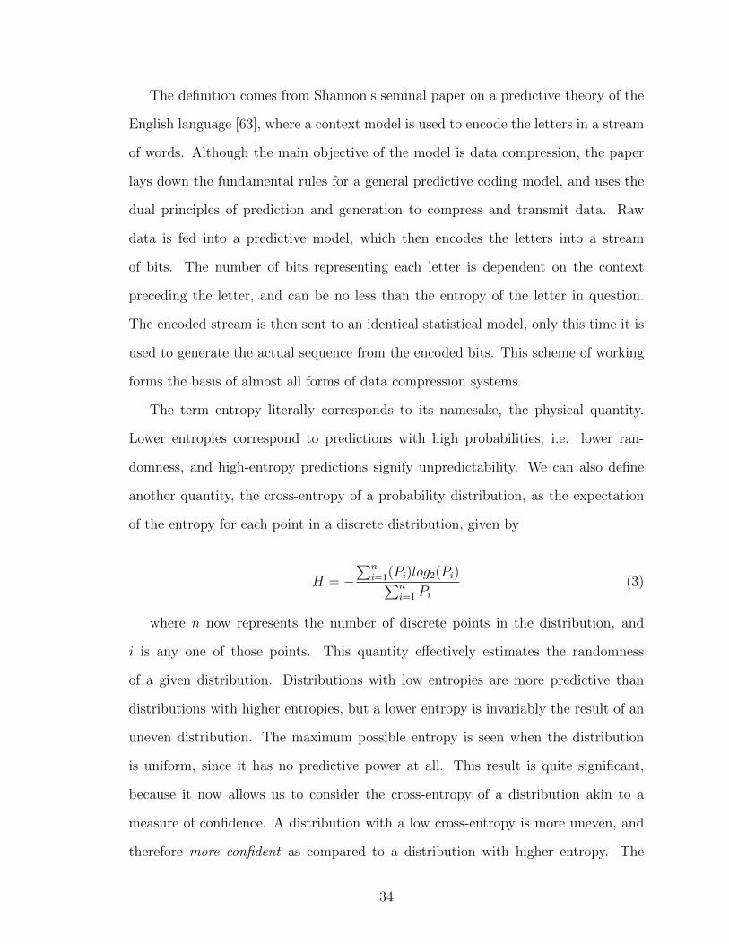
The definition comes from Shannon’s seminal paper on a predictive theory of the
English language [63], where a context model is used to encode the letters in a stream
of words. Although the main objective of the model is data compression, the paper
lays down the fundamental rules for a general predictive coding model, and uses the
dual principles of prediction and generation to compress and transmit data. Raw
data is fed into a predictive model, which then encodes the letters into a stream
of bits. The number of bits representing each letter is dependent on the context
preceding the letter, and can be no less than the entropy of the letter in question.
The encoded stream is then sent to an identical statistical model, only this time it is
used to generate the actual sequence from the encoded bits. This scheme of working
forms the basis of almost all forms of data compression systems.
The term entropy literally corresponds to its namesake, the physical quantity.
Lower entropies correspond to predictions with high probabilities, i.e. lower ran-
domness, and high-entropy predictions signify unpredictability. We can also define
another quantity, the cross-entropy of a probability distribution, as the expectation
of the entropy for each point in a discrete distribution, given by
H = −∑n
i=1(Pi)log2(Pi)∑ni=1 Pi
(3)
where n now represents the number of discrete points in the distribution, and
i is any one of those points. This quantity effectively estimates the randomness
of a given distribution. Distributions with low entropies are more predictive than
distributions with higher entropies, but a lower entropy is invariably the result of an
uneven distribution. The maximum possible entropy is seen when the distribution
is uniform, since it has no predictive power at all. This result is quite significant,
because it now allows us to consider the cross-entropy of a distribution akin to a
measure of confidence. A distribution with a low cross-entropy is more uneven, and
therefore more confident as compared to a distribution with higher entropy. The
34

Figure 4: Sketch showing the relationship between the probabilities in a finite dis-tribution (the yellow lines) and the entropy of the distribution (represented by thered lines). The distribution on the left has a lower entropy because it has one clearprediction.
inverse of the cross-entropy H of a distribution is used as a measure of confidence, to
decide the which viewpoints deserve more weight in the merging process.
3.4.2 Merging Viewpoints
The process of combining the predictions of the different viewpoints is simply a
weighted average of all the predictive distributions, where the weights for each dis-
tribution depend upon its entropy. The weight for each distribution is given by a
normalized average across the entire distribution.
wm =H(pm)
Hmax(Pm)(4)
Higher average entropies result in lower weights for the distribution, this way in
the final merging process, viewpoints that are less confident (having higher entropies)
make much smaller contributions to the final prediction. This allows us to choose the
best predictions depending on the context of the event, leading to better matches and
lower entropies for the model as a whole.
35

3.4.3 Perplexity
For the purpose of evaluating the performance of a model, we also use another metric,
perplexity, defined as 2 raised to the power of the entropy. While entropy represents
the minimum bound of the number of bits used to encode the occurence of that event,
the perplexity is simply another way of looking at the same measure. The perplexity
of an event is an estimation of the number of uniform choices that the model is faced
with in the prediction of that event. Since the perplexity of a model is mapped to an
exponential scale, it increases very rapidly as the probability decreases, making it a
good metric to amplify the differences in predictions with small probabilities. In fact,
most of our results are expressed using perplexity since it makes them a little easier
to read and understand.
36

CHAPTER IV
VLMM IMPLEMENTATION
The system is implemented as a MAX/MSP object and is written in C++. MAX/MSP
was chosen as the platform for development because of its vast library of pre-built
objects and libraries. It provided the flexibility to design and run a variety of tests
over the entire database, making it easy and efficient to change parameters between
test runs, with the patches being completely re-usable for the VLHMM as well. This
chapter describes the details of this implementation of an integrated VLMM frame-
work that makes use of all the concepts discussed until now to model a set of tabla
compositions, leading to two conference publications [13, 15]. It involves designing
an MVM, finding the relevant viewpoints, and designing an evaluation scheme that
returns an accurate description of the performance of the model. The first step in
this process is the creation of a training database.
4.1 **bol Database
The VLMM system is trained on a symbolic database, encoded from Aloke Dutta’s
book of tabla compositions [30]. The book is a tutorial for novice tabla players,
outlining the basic principles of improvisation on the tabla using transcriptions of
various forms of improvisations. The book also lists some renowned fixed composi-
tions, which were also incorporated into the database. In total, it contains 34 songs
of 8 different types - 13 Qaidas, 5 Relas, 4 Tukdas, 4 Gats, 4 Chakradars, 2 Keharva
thekas, 1 Dadra and 1 Laggi. An important point to note here is that about 50% of
the database is comprised of qaidas and relas, which are both improvisational forms,
based around a central theme. The database comprises these 34 songs - a total of
27,189 strokes, using 42 unique symbols. These songs were encoded manually from
37
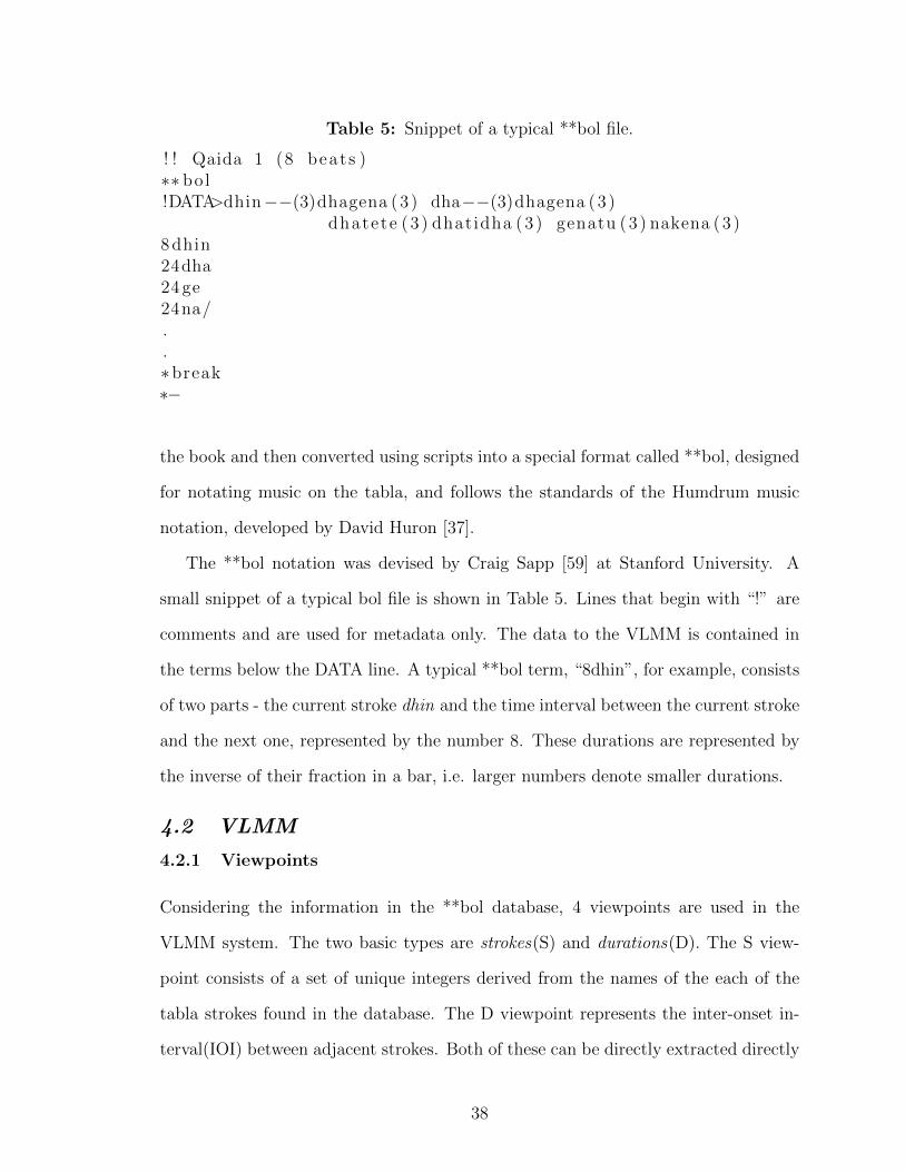
Table 5: Snippet of a typical **bol file.
! ! Qaida 1 (8 beats )∗∗ bol!DATA>dhin−−(3)dhagena (3 ) dha−−(3)dhagena (3 )
dhatete (3 ) dhatidha (3 ) genatu (3 ) nakena (3 )8 dhin24dha24 ge24na/..∗break∗−
the book and then converted using scripts into a special format called **bol, designed
for notating music on the tabla, and follows the standards of the Humdrum music
notation, developed by David Huron [37].
The **bol notation was devised by Craig Sapp [59] at Stanford University. A
small snippet of a typical bol file is shown in Table 5. Lines that begin with “!” are
comments and are used for metadata only. The data to the VLMM is contained in
the terms below the DATA line. A typical **bol term, “8dhin”, for example, consists
of two parts - the current stroke dhin and the time interval between the current stroke
and the next one, represented by the number 8. These durations are represented by
the inverse of their fraction in a bar, i.e. larger numbers denote smaller durations.
4.2 VLMM
4.2.1 Viewpoints
Considering the information in the **bol database, 4 viewpoints are used in the
VLMM system. The two basic types are strokes(S) and durations(D). The S view-
point consists of a set of unique integers derived from the names of the each of the
tabla strokes found in the database. The D viewpoint represents the inter-onset in-
terval(IOI) between adjacent strokes. Both of these can be directly extracted directly
38
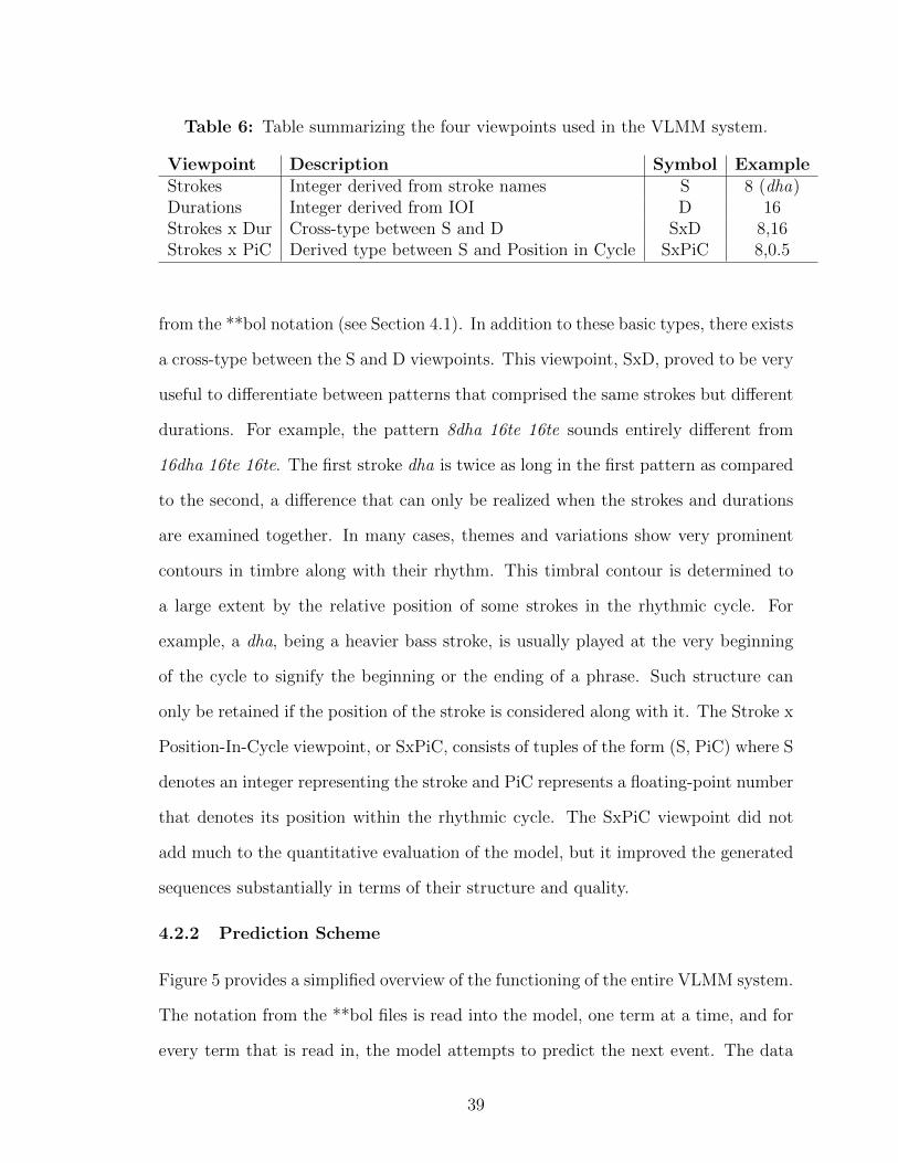
Table 6: Table summarizing the four viewpoints used in the VLMM system.
Viewpoint Description Symbol ExampleStrokes Integer derived from stroke names S 8 (dha)Durations Integer derived from IOI D 16Strokes x Dur Cross-type between S and D SxD 8,16Strokes x PiC Derived type between S and Position in Cycle SxPiC 8,0.5
from the **bol notation (see Section 4.1). In addition to these basic types, there exists
a cross-type between the S and D viewpoints. This viewpoint, SxD, proved to be very
useful to differentiate between patterns that comprised the same strokes but different
durations. For example, the pattern 8dha 16te 16te sounds entirely different from
16dha 16te 16te. The first stroke dha is twice as long in the first pattern as compared
to the second, a difference that can only be realized when the strokes and durations
are examined together. In many cases, themes and variations show very prominent
contours in timbre along with their rhythm. This timbral contour is determined to
a large extent by the relative position of some strokes in the rhythmic cycle. For
example, a dha, being a heavier bass stroke, is usually played at the very beginning
of the cycle to signify the beginning or the ending of a phrase. Such structure can
only be retained if the position of the stroke is considered along with it. The Stroke x
Position-In-Cycle viewpoint, or SxPiC, consists of tuples of the form (S, PiC) where S
denotes an integer representing the stroke and PiC represents a floating-point number
that denotes its position within the rhythmic cycle. The SxPiC viewpoint did not
add much to the quantitative evaluation of the model, but it improved the generated
sequences substantially in terms of their structure and quality.
4.2.2 Prediction Scheme
Figure 5 provides a simplified overview of the functioning of the entire VLMM system.
The notation from the **bol files is read into the model, one term at a time, and for
every term that is read in, the model attempts to predict the next event. The data
39

8te**bol notation
Strokes (S)
te 8 te, 8 te, 2
dha te na dha,8 te,8 na,44 8 dha,2 na,2
8dha
Merged DistributionNext Event
Long Term
Short Term
+
Dur (D)
S x D
S x PiC
Figure 5: Figure showing an overview of the prediction scheme used in the VLMM.
40

is first split into the different viewpoints, and each viewpoint constructs two PSTs -
a Long Term Model(LTM) and a Short Term Model(STM). The LTM is constructed
during the training phase of the model, on 33 out of the 34 available compositions,
while the STM is constructed on testing data, i.e. the one remaining composition.
The reason for constructing two PSTs instead of a single one, is to balance the
amount of repetition with the extent of variation. A typical tabla composition, like a
qaida, is built around a theme variation structure, where each song consists of its own
characteristic patterns and motifs. A large database, such as the LTM is unaware of
such local details due to the sheer number of possible variations available to it. In
other words, it is too general to be of any use to a particular song, and many obvious
repetitions are easily missed by the LTM. The STM however, is constructed on this
one song alone, and is able to identify these repeating motifs very easily. When a
prediction is called for, each viewpoint, therefore, makes use of both models, merging
their individual distributions into a single one. These distributions are merged yet
again before a final prediction is made. Note how the SxD and SxPiC viewpoints can
alter the distributions returned by the S or D viewpoints.
Let us take another look at the PST discussed in Section 3.3 in Figure 3. Let
us assume that this PST is built on a sequence of strokes, S = {dha, ge, na, ge}.
Now, assume we are given a sequence S ′ = {dha, ge} and asked to predict the the
probability of na being the next term in this sequence. We start by considering
sequences of all orders less than the given sequence S ′, upto the maximum order N
with the term na appended to the sequence. This gives us S ′0 = {na}; S ′1 = {ge, na}
and S ′2 = {dha, ge, na}. The probability of na following the sequence S ′ is given by
P (na) =P (S ′0) + P (S ′1) + P (S ′2)
3(5)
which is simply the sum of the probabilities of all possible pathways for the PST
to generate a na. We can now rewrite equation 5 as
41

P (na) =P (na|{}) + P (na|{ge}) + P (na|{dha, ge})
3(6)
This is where the smoothing scheme is used. Applying the weights from the
smoothing scheme to the PST, this now becomes
P (na) =w0P (na|{}) + w1P (na|{ge}) + w2P (na|{dha, ge})
w0 + w1 + w2
(7)
so that the final probability is the weighted sum of the probability of the term na
at different levels of the PST. We can now generalize this to derive a single equation
that describes the process for each prediction with in the VLMM:
P (xn+1|{x0 . . . xn}) =w0P (xn+1|{}) + w1P (xn+1|{xn}) +
∑ni=2wiP (xn+1|{xn−i+1 . . . xn})∑N
i=0wi
(8)
Thus a VLMM of order N is equivalent to combining the predictions of all fixed-
order Markov models from order 0 to N. This process occurs for both the LTM and
STM of every single viewpoint whenever a prediction is called. The basic architecture
of the PST was designed by Trishul Mallikarjuna from the Georgia Tech Center for
Music Technology. A large part of it has changed considerably over the course of
this work, but some parts still remain as they were. His help in this regard is greatly
appreciated. There are still two details about the PST that must be made clear before
we can proceed with the merging scheme for the viewpoints - the escape probabilities
and the smoothing scheme.
4.2.2.1 Escape probabilities
Witten and Bell, in their work on tackling the zero-frequency problem [68], provide
a quantitative comparison between the different methods used to address the zero-
frequency problem in modern data compression algorithms. Since each PST in the
42

VLMM system is a context dependent model, not unlike a predictive coding model,
the approach deemed to be the most effective by Witten and Bell was chosen for this
work as well. The Poisson process model, as it is called, is a method for estimating the
escape probabilities of a model based on the number of terms in the training set and
their frequency. In very simple terms, the escape probability for a given model (for a
level of the tree, in our case) increases along with the ratio of new terms encountered
to the total number of terms.
Let us assume that out of an unknown number q of unique tokens, we have en-
countered ci of type i, in a sample set of size n. Assuming that these tokens of
type i occur according to a Poisson process, the expected probability that the next
encountered event will be novel is given by
ε =t1n− t2n2
+t3n3− . . . (9)
where ti is the number of unique terms that have occurred i times. Now assuming
that we are dealing with a reasonable amount of repetition in our sample set, and
given that n is sufficiently large, we can neglect the higher terms of the series shown
in equation 9 and approximate this to ε = t1/n. Since n needs to be large enough,
we apply these escape probabilities to all sequences of a specific order, like we would
if we were maintaining separate Markov models for each order of the VLMM instead
of a PST. We can now define the escape probability at each level of the tree as:
εn =t1nNn
(10)
for the nth level of the tree. N is the total number of sequences of length n and
t1n represents the number of terms at the nth level that have been seen only once.
43

4.2.2.2 Smoothing
The smoothing process used in a PST decides the ratio of weights w0 . . . wn in equation
8. Based on the results of a study of smoothing algorithms for language models by
Chen and Goodman [12], two basic approaches were implemented for the VLMM -
the Kneser-Ney and the 1/N smoothing schemes.
The Kneser-Ney [40] smoothing scheme is essentially a discounting scheme that
sets the weight for a given level of the tree based on certain pre-assigned discount
factors for each level. The weight assigned to each level of the tree depends on the
number of elements that have occurred once or more, along with the weighted sum
of the discount factors of all previous levels of the tree. The scheme assigns higher
weights to those levels of the tree that show more repetition. A full explanation of
the scheme is beyond the scope of this document, however, [12] and [40] both provide
very accurate descriptions of the process.
On the other hand, the 1/N approach, assigns weights to each level of the tree
using a fixed-weight scheme designed to give more priority to higher orders regardless
of the amount of repetition at each level. The weight for the ith level of a tree of
maximum order N is given by
wi =1
N − i+ 1(11)
Surprisingly, a formal comparsion between the 1/N and Kneser-Ney schemes (de-
scribed in Section 4.4) showed that the 1/N approach performed much better than the
Kneser-Ney approach in terms of the entropies of the predicted output, despite being
much simpler. One reason for this could be that the Kneser-Ney approach is designed
for words in sentences, which almost always will have fewer repetitions than musical
phrases, thus overcompensating for the amount of repetition in a theme-variation
composition. The results of these comparisons prompted a third smoothing scheme,
44

1 5 100
0.2
0.4
0.6
0.8
1
Order of the model
Wei
ght
x = 0x = 0.5x = 1x = 2x = 1/Nx = 5x = 10x = 100
Figure 6: Figure showing the family of curves represented by the Parametric smooth-ing scheme.
intended to be a much broader look at how smoothing affects the resulting entropy
distribution of a context model. A generalized form of the 1/N scheme was designed
and implemented by Aaron Albin and myself. We call it the parametric weighting
scheme (denoted by P), based on a family of curves of the form
wi = a
{(1− c
a
)( i
N
)x}+ c (12)
By adjusting the values for the amplitude (a), the offset (c) and the exponent
(x), the weights can be shifted, allowing the model to choose between more specific
matches or general predictions. Figure 6 shows the range of curves that can be
produced using this weighting scheme. We, Aaron and I, set out to explore two
potential questions here. Firstly, how much of an effect did these parameters actually
have on the system? And second, is there an optimum set of values for a, b and x
that would give us the best results in terms of cross-perplexity?
To address these questions, we trained a VLMM model of maximum order 10
45

and compared the cross-entropy results between the 1/N system and the parametric
system, with different values of the exponent value (x) ranging from 0 to 100. We
also compared these models against a simple back-off (BO) model that would consider
only the longest context match possible. In addition, we used the data from these
trials to hone in on an optimum set of parameters.
4.2.3 Merging Predictions
When a prediction is called for, all the information gathered so far has to be inte-
grated and presented to the user in the form of basic types, i.e. the next stroke and
its corresponding duration. The first step is merging the LTM and the STM for each
viewpoint to get a combined prediction. Once this is done, the distributions returned
by individual viewpoints are merged again. The merging scheme for both these pro-
cesses is identical, making use of the cross-entropy of the distributions to decide the
weightage for each.
Suppose we have two viewpoints V1 and V2, whose respective distributions must be
combined. The cross-entropy of each distribution is first calculated using the relation
H = −N∑i=1
Pilog2(Pi) (13)
The next step is the normalization of this measure by the maximum entropy of
the distribution Hmax, which is obtained by taking the negative logarithm of the
minimum probability in the distribution, denoted by Pm. This returns the weight
associated with that distribution.
wm =H
Hmax(Pm)(14)
The actual process of merging is simply a point-by-point weighted average of the
two distributions. For the basic types, strokes and durations, the combined prediction
of the LTM and the STM is returned as the final distribution. For the SxD viewpoint,
46

the combined distribution has to be marginalized and split into two distributions
- one corresponding to strokes, and another corresponding to durations. Each of
these distributions is then merged with its corresponding basic type. The derived
viewpoints SxPiC demands some explanation. We decided not to use this viewpoint
in the LTM, mainly because different compositions used different time signatures and
rhythmic accents, and incorporating this viewpoint in such a diverse database would
cause more harm than good. This viewpoint was only used in the STM to preserve the
rhythmic structure specific to each piece. At each prediction, the position in the cycle
is checked and a distribution for all strokes occuring at this position is returned. This
distribution is then merged with the strokes viewpoint. The S and D distributions
are then normalized so that cross-entropy can be calculated.
4.3 Evaluation
Perplexity, which is in turn derived from entropy, is used as the metric to evaluate
model accuracy and performance. A leave-one-out cross-validation scheme is used
at the song level. For each run, 33 out of the 34 songs are used as training data to
build up the VLMMs for the LTM. The remaining song is then fed in token by token
and a prediction is called at every step before the token is actually fed to the STM.
The model returns a probability distribution for that time-step and the entropy for
the actual testing token at that step is checked and recorded. This is repeated for
every song until the log contains a set of entropies corresponding to every token in
the database. These entropies are then averaged and the average entropy is converted
to perplexity. If the model has been trained well, the average perplexity across all 34
runs should be relatively low. Recall Shannon’s original definition of the entropy EL
of a language L
EL = −∑n
i=1 log2(P (ei|ci)n
(15)
47

where ei is the ith event occurring after its corresponding context ci and n is the
total number of subsequences used in the estimation process. This is exactly what we
use to estimate the performance of our model. A lower EL means a better predictive
theory, which means that we also have a better generative system. Note that the
measure EL represents the average of the entropy values for each prediction; it should
not be confused with the cross-entropy of a distribution H (Eqn. 13. EL is used to
measure the performance of the model, whereas H is used to assign weights to each
of the models before the merging process.
This system of evaluation was used to test the performance of the model over a
variety of experiments. The first of these is a comparison of the average entropies
of the LTM, STM and their combined prediction for orders ranging from 1 to 20.
It conveys the relationship between entropy (or perplexity) and model order, and
highlights the difference in predictions between the corpus-wide VLMM of the LTM,
and the song-specific STM. The impact of different smoothing schemes for a VLMM
of order 10 was also studied using a detailed study of the average entropy of each
viewpoint under each smoothing scheme. The results establish the trend of decreasing
entropy as the number of viewpoints are increased, and also show which smoothing
scheme works best for each viewpoint. To add to this, a separate study on the
parametric model alone shows that its exponent value can be tuned to minimize the
average entropy for given system.
4.4 Results
Figure 7 shows the change in the average perplexity of the VLMM with the change in
the maximum order. As you can see, there is a clear downward trend in the values,
with the LTM Order 0 showing an entropy of 3.614 (perplexity of 12.24) and Order
20 shallowing out at an entropy of 1.584 (perplexity of 3.0). Results are statistically
significant at the 0.01 level. Clearly, increase in the model order leads to better
48

0 5 10 15 20 250
1
2
3
4
5
6
Order
Cro
ss−
En
tro
py
Priors Combined STM LTM
Figure 7: Entropy of predictions plotted against increasing model order
performance, although with diminishing returns. Beyond this limit (Order 20), even
drastic increases in the model order caused only negligible changes in perplexity, and
so we did not pursue this any further. The drop in perplexity can be easily explained
by considering the nature of the task at hand. Over 42 symbols, the chance of picking
any one of them randomly is only about 1/42 or 2.3%. As soon as some context
information is provided to the system, most of these possibilities get filtered out, and
number of valid paths that could continue the sequence gets considerably smaller.
This leads to a sharp decrease in the average perplexity from Order 0 to Order 1. As
we go deeper and deeper down the PST, however, we start reaching the limit of the
sequences that have actually been seen by the model so far. In fact, a large number
of songs in the database are built around sequences that are 16 beats long, leading to
about 32 strokes for a many of the sequences. At around Order 30 and beyond, the
PST is reaching the limits of its sequence length, and further increases to say, 40 or
50 make no difference to the model. Moreover, exact matches are extremely difficult
to find for higher orders, therefore, the model ends up picking possibilities from lower
orders instead, leading to only marginal improvements for these higher orders. The
49

increase in order also led to noticeable changes in the generative aspect of the model,
and higher-order models tended to produce larger fragments of coherent material,
as we would expect. Beyond order 20 though, differences in the musical material
produced were no longer easily noticeable.
Along with the experiment discussed above, an informal qualitative evaluation of
the musical material generated by the VLMM was also conducted. This evaluation
was very brief and completely subjective, based only on the opinions of Dr. Chordia
and myself, and therefore will not be described here. However, it did yield two useful
results that influenced some technical decisions that deserve mention. The first is that
although the STM seems to show lower entropies than the LTM and the combined
model (see Figure 7), its generative output tends to be very repetitive. The combined
model, on the other hand, may show a higher average entropy but tends to produce
more interesting phrases and variations. This means that the LTM provides the
variety for creating novel variations, while the STM provides the structure to help
keep the composition coherent. A corollary of this is that since the STM is getting
trained as each song progresses, the entropy per term tends to decrease over time,
flattening out after approximately 50-100 tokens (a theme and one or two variations
worth). This indicates the minimum amount of material required for the STM to
incorporate the song-specific structure. The second result is that the SxPiC viewpoint
caused a surprising amount of improvement in the coherence of the generated phrases
by preserving the rhythmic structure within a theme or variation. Although this
improvement is not visible in the quantitative results, from a practical standpoint,
the SxPiC viewpoint is essential to the phrase generation process of the VLMM.
A variety of experiments were conducted to compare the relationship between
smoothing algorithms and model performance. Table 7 summarizes the results for
the Back-Off(BO) model, 1/N approach(1/N) and the Parametric(P) model using a
VLMM of maximum order 10. The BO model is clearly the least effective of the
50

Table 7: Average and median of perplexity results for for back-off, 1/N, and paramet-ric (with exponent coefficient equal to 1) smoothing methods. Results for combinedmodels using a maximum order of 10. MV refers to the multiple-viewpoints model inwhich the SxD and SxPIC viewpoints have been incorporated.Model Strokes Strokes MV Durations Durations MV SxD SxPIC
Av. Med. Av. Med. Av. Med. Av. Med. Av. Med. Av. Med.
BO 2.71 1.08 2.41 1.07 2.11 1.014 1.83 1.01 3.84 1.29 2.58 1.40
1/N 2.08 1.37 1.80 1.19 1.44 1.11 1.30 1.06 2.69 1.58 2.55 1.37
P (x=1) 2.00 1.33 2.03 1.27 1.55 1.09 1.42 1.07 2.60 1.43 2.57 1.37
Table 8: Summary of perplexity results for LTM for order 10.
Order Durations Strokes SxD
10 1.76 3.05 4.66
three, however, it still gives the lowest values for median perplexity. This suggests
that the BO model tends to either find very good matches, or not at all, while the
other two models manage to strike a better compromise because of their weighting
schemes. Figure 10 shows us a histogram of all perplexity values for the BO model. As
expected, there is a large concentration of values around 0, however, the distribution
continues till values of 30 or more. Between the other two models, the parametric
model, with an exponential coefficient of 1 (denoted P(x=1)) seems to do marginally
better than the 1/N model, though not always. Figure 4.4 gives us a much better
look at the differences between the BO model and the 1/N model for the different
viewpoints. All models however, compare very favorably to the baseline perplexity of
12.24 obtained using only the prior probabilities of the independent strokes.
Another trend that relates to Table 7 is regarding the drop in perplexity with
the addition of viewpoints. Reading across the table, we see that the addition of
viewpoints seems to improve model performance. For the BO model, perplexity
drops from 2.71 to 2.41 between Strokes and Stroke MV, meaning that the addition
of the SxD viewpoint to the Strokes viewpoint brought some useful information to
the table. The same trend is also seen between Durations and Durations MV for the
51

Strokes MV Durations MV Strokes Durations0
0.5
1
1.5
2
2.5
3
Aver
age
Cro
ss−P
erpl
exity
BO1/N
(a) Comparison of average perplexity betweenBO and 1/N for single and multiple viewpoints.
Strokes MV Durations MV Strokes Durations0
0.2
0.4
0.6
0.8
1
1.2
1.4
Med
ian
Cro
ss−P
erpl
exity
BO1/N
(b) Comparison of median perplexity betweenBO and 1/N for single and multiple viewpoints.
Figure 8: Comparison of perplexity between BO and 1/N models.
BO model. Again, all the results discussed so far are statistically significant on the
Tukey-Kramer test at the 0.01 level.
Figure 9 shows the variation of average perplexity for different values of the expo-
nent for the parametric model. The curves points towards a minima between x = 0.5
and x = 2, an optimum value of the exponent within this range. The results show
that the weighting scheme does make a small but significant difference to the pre-
diction scheme of the model. Clearly, higher weights for higher orders leads to lower
perplexities, though this rule does not hold beyond a certain limit. What is not seen
here is the effect of changing the smoothing scheme on individual predictions. Though
the average perplexities might not vary too much, it might lead to subtle changes in
prediction and generation. It might be worthwhile to explore the effect of smoothing
in a generative context rather than in a quantitative analysis.
52

0 0.5 1 2 5 10 1001.4
1.6
1.8
2
2.2
2.4
2.6
2.8
3
Exponent of Parametric Model
Ave
rage
Per
plex
ity
Durations Strokes Dur−Stroke Stroke−PIC
Figure 9: Perplexity as a function of exponent coefficient in parametric model. Thereseems to be an optimal range between 1 and 2.
0 5 10 15 20 25 30100
101
102
103
104
Cross−Entropy
log(Distribution)
Figure 10: Histogram showing range of perplexity values when predicting strokes forthe Back-Off model
53
CHAPTER V
VLHMM IMPLEMENTATION
The model described so far only handles symbolic data, and while there are plenty of
applications for such a model, a more practical scenario would be to try and apply
these principles to audio data. This involves using VLHMMs instead of VLMMs,
applying the principles learnt using the VLMM to the audio domain. The transition
from symbols to audio is not a very simple one has some major consequences on the
system as well as its behaviour.
5.1 Hidden Markov Models
The extension from Markov models to Hidden Markov models is one that was born
out of practical necessity. While symbolic information is a useful source of input, it
is not always available. In most cases, what is available is real-world data such as
sensor measurements like raw audio input from a microphone, or acceleration from
accelerometers. HMMs provide the means to apply sequence modeling effectively to
real data. They have proven to be very successful for applications such as speech
recognition and music information retrieval. Juang and Rabiner explain the power
behind HMMs and their success in speech processing in their seminal paper on first-
order HMMs [39]. Thede and Harper describe the use of a second-order HMM in [65].
In MIR applications, HMMs have proved to be quite successful at chord estimation
and key extraction [42] [43] and automatic accompaniment for vocal melodies [11].
Figure 11 gives a simplified explanation of the concept behind an HMM. Consider
the Markov model described in Figure 2. Recall that it shows the transition probabil-
ities to predict whether the next day is going to be sunny or rainy, depending on the
54
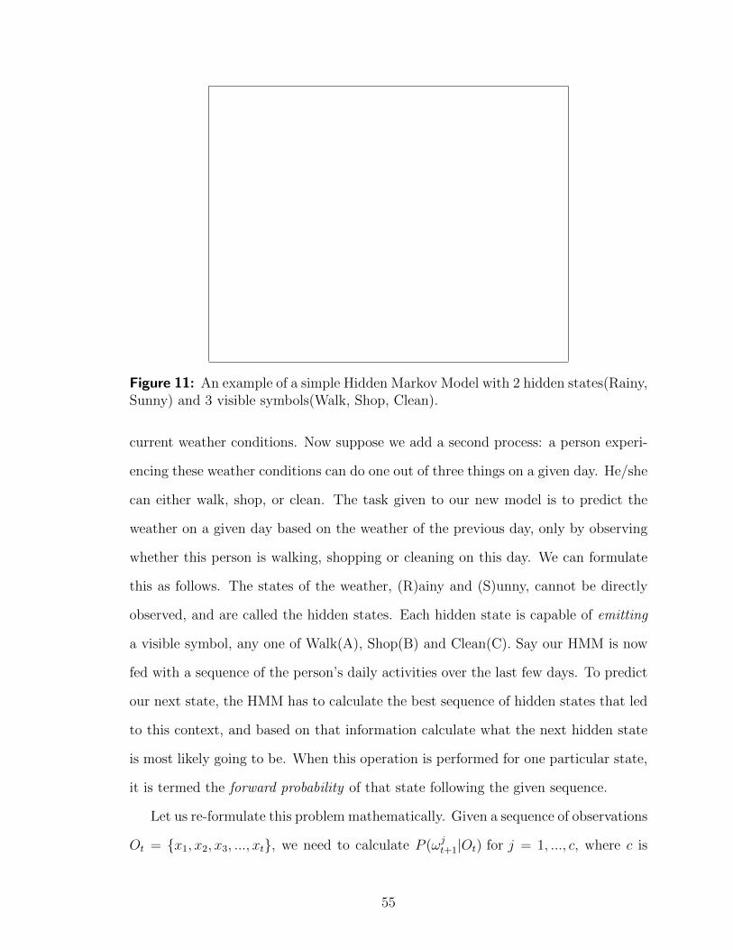
Figure 11: An example of a simple Hidden Markov Model with 2 hidden states(Rainy,Sunny) and 3 visible symbols(Walk, Shop, Clean).
current weather conditions. Now suppose we add a second process: a person experi-
encing these weather conditions can do one out of three things on a given day. He/she
can either walk, shop, or clean. The task given to our new model is to predict the
weather on a given day based on the weather of the previous day, only by observing
whether this person is walking, shopping or cleaning on this day. We can formulate
this as follows. The states of the weather, (R)ainy and (S)unny, cannot be directly
observed, and are called the hidden states. Each hidden state is capable of emitting
a visible symbol, any one of Walk(A), Shop(B) and Clean(C). Say our HMM is now
fed with a sequence of the person’s daily activities over the last few days. To predict
our next state, the HMM has to calculate the best sequence of hidden states that led
to this context, and based on that information calculate what the next hidden state
is most likely going to be. When this operation is performed for one particular state,
it is termed the forward probability of that state following the given sequence.
Let us re-formulate this problem mathematically. Given a sequence of observations
Ot = {x1, x2, x3, ..., xt}, we need to calculate P (ωjt+1|Ot) for j = 1, ..., c, where c is
55
the number of hidden states, and P (ωjt+1) represents the probability of the jth state
at time t+ 1. This is simply P (ωjt+1|Ot) =
∑ci=1 α
tiaij, where αt
i is the probability of
being in state i at time t having emitted Ot, i.e. the forward probability of state i.
If aij is the probability of making a transition from i to j then the required forward
probabilities can be calculated recursively as follows:
αtj =
c∑i=1
αt−1i aijP (xt|ωj) (16)
giving us the probability of state j occurring after the sequence Ot has been
emitted. This needs to be repeated for every possible state, to calculate a discrete
distribution across all hidden states.
5.2 Database
A synthetic audio database based on the symbolic **bol files described in Section
4.1 was generated for the purpose of evaluating the VLHMM. Two sets of files were
recorded, each using a different set of samples, for training and testing. The samples
were taken from two previously recorded performances by renowned tabla players.
These recordings were part of a previous experiment [14] and had already been seg-
mented into strokes and labelled manually. The **bol files were then used to syn-
thesize the compositions stroke by stroke. To achieve this, a tabla stroke sequencer,
designed in PureData, by Alex Rae as part of his thesis [55], was used - stroke labels
and IOIs were read from **bol files and the corresponding stroke samples were trig-
gered in sequence. The resulting audio was recorded as wav file (16-bit, 44.1 kHz). A
randomized selection process was used to choose between about 10 different samples
for each stroke to increase the variability and difficulty of classification. For each
song, the timestamps of each stroke were also noted. The audio, timestamps as well
as the bol files were organized into separate folders and now form the JNMR Tabla
Database. It is accessible at http://paragchordia.com/jnmrTabla.
56

Using the recorded time-stamps, the audio files were programmatically segmented
into individual strokes and read into MATLAB. Sertan Senturk’s help with this part
of the process proved to be invaluable. His code on segmentation and feature ex-
traction was instrumental for the timely completion of this work. Although beat
detection could have been employed to segment the files, which would allow us to
model durations as well, in the interest of time, we decided to use the time-stamps
for the segmentation process. It remains for future work to implement an onset de-
tection system for the HMM. Based on [33], we found that the MFCCs were a good
choice of features for percussive samples and the first 21 MFCCs were extracted for
each of the strokes. The 0th coefficient, representing signal energy was discarded. On
average, the length of each sample was within about half a second, so the features
were calculated on the entire stroke, without any division into frames. This resulted
in a longer FFT length than a standard such as 4096 samples, therefore offering very
high frequency resolution for the features. On the symbolic side, the 42 stroke names
were re-mapped to 9 acoustic categories. Several strokes used different names depend-
ing on their context in the composition. To simplify the task of audio classification,
similar sounding strokes were grouped into the same acoustic category and a new set
of labels was prepared. The features were then aligned with their respective labels
and written to another set of files which were then read in to the VLHMM system.
The reason for creating a synthetic database, instead of original recordings, is
that we wanted a database that was annotated on a stroke-by-stroke basis. Since the
symbolic database provided the names of the strokes for us, it was easier, both in terms
of time and effort, to synthesize a new database instead of manually annotating a the
recordings. The synthesized database also has the advantage of having a much larger
number of strokes because the recordings were only a couple of hours in length. The
use of a synthetic database usually produces optimistic results since the variations
within a small synthesized set are much smaller than those encountered in a real
57

scenario. This is accounted for by the use of two completely different sets of samples
for the training and testing database. This should simulate a a real-world case, where
the model has no prior information about incoming audio.
5.3 VLHMM
The VLHMM framework is built upon the PST architecture developed for the VLMM,
however, the complexity of a VLHMM system led to considerable differences between
the two models. The first of these, is that the **bol input to the model is now replaced
by feature vectors extracted from segmented audio samples. The audio features also
add an additional layer into the predictive process - not only do we have to try and
predict what stroke comes next, we also have to evaluate the probability of the input
features representing that stroke. The PST itself is re-designed to accommodate two
distributions instead of one - every node in the tree contains a transition probability
for the state itself, and an emission distribution for the visible symbols. To add to
this, the state space for the visible symbols is a continuous spectrum consisting of
the entire range of MFCC values, and not a discrete space. Therefore, the emission
distribution consists of a multi-variate gaussian(MVG) mapping all observed values of
the MFCCs into all observed stroke types. The biggest consequence of these changes is
processing time. There is a massive amount of computation required to calculate the
forward probability of each sequence, and this computation increases exponentially as
we go down the tree. At the same time, a significant amount of uncertainty is added
to the system by the continuous input, causing a noticeable decrease in performance.
Another change in the VLHMM is the reduction in the state space - the number
of strokes - from 42 to just 9. There are two reasons for this, the first being that the
system of nomenclature of the tabla is based on bols and not the strokes themselves.
Since a bol is a compositional unit, rather than a specific sound, the same stroke can
be represented by several different bols depending on its position in the piece. Since
58

the model has no way of differentiating these bols by their acoustic features, all bols of
similar acoustic properties were grouped together into a single stroke. This reduced
state space also has the added benefit of reducing the computation time drastically.
The final change, in a effort to reduce the calculation time taken per prediction, the
VLHMM model does not use the STM. The inclusion of the STM would double the
time taken per prediction, making the model too slow for any practical purpose, so
it was decided that only the LTM would be used, and the order of the model would
be restricted to a maximum of 3.
The remaining aspects of the VLMM structure are kept as they are. All low-level
data structures and functions are retained except for minor changes to accommodate
the new input types. Higher level functions such as those used for building the PST -
smoothing, merging and prediction - remain largely unchanged, and all the concepts
developed for the VLMM are adapted to the architecture of the HMM.
5.3.1 Training
The training procedure for the HMM is comprised of two independent processes. The
first involves creating the MVG system for the set of strokes. We used a leave-one-
out approach as before, creating 34 sets of MVGs, each one built without using the
strokes of one of the songs. Each MVG was built using the MFCC coefficients of
the strokes using a shared covariance matrix. The means and covariances were then
written to files and read in directly into the VLHMM. The second process involves
building the PST. This was done exactly as before, since we are only using stroke
labels to estimate the transition probabilities between the nodes of the PST. Here,
we use the same emission distribution for all nodes of the tree.
5.3.2 Prediction Scheme
Prediction for the VLHMM is almost identical to the process used for the VLMM.
As discussed in Section 5.1, the probability of a state, or in our case, a stroke, ωjt+1
59

is given by
P (ωjt+1|Ot) =
c∑i=1
αtiaij (17)
Note that this probability is only for a single HMM of a fixed order. For a VLHMM
system, all subsequences of the original sequence must also be considered and their
weighted sum is then taken. This now gives us the equation
P (ωjt+1) =
w0P (ωjt+1|{}) + w1P (ωj
t+1|{xt}) +∑N−1
i=2 wiP (ωjt+1|{xt−i+1, . . . , xt})∑N−1
i=0 wi
(18)
which returns the probability that the stroke ωj is going to occur at time t + 1.
This process is then repeated for all possible symbols and the resulting distribution
is then normalized to sum up to 1. The probabilities are then converted to entropies
and averaged as part of the evaluation proces.
However, as noted earlier this quickly becomes unmanageable because the state
space expands rapidly for high-order models. The PST architecture, provides a prac-
tical solution and allows us to consider a much smaller number of terms in the calcu-
lation of each forward probability αit. To calculate P (ωj
t+1|Ot), for an HMM of order
m, we look for all nodes at level m+ 1 that correspond to category j. Let the set of
such nodes be A. The total number of nodes that fit this definition will be the number
of terms in our sum, which will in general be much less than the theoretical maxi-
mum. Since each node has only one parent, we multiply the forward probability of
the parent node by the transition probability from the parent to child. These partial
probabilities are then summed for all i ∈ A to get P (ωjt+1). In other words, we now
have αtj =
∑i∈A α
t−1i aijP (xt|ωj). Figure 12 shows how the number of nodes grows
with the depth of the tree for this data set compared with the theoretical maximum
60

given by cm. Between order 2 and 3 the number of possible nodes explodes, how-
ever the actual number of nodes in the PST is approximately an order of magnitude
less than this. Another caveat with high-order HMMs is that labeled symbolic data
might not always be available and so the training process comes down to estimating
the transition probabilities between the states using the Baum-Welsch algorithm [6].
In this case, since the hidden states correspond to the strokes, and that information
was easily available, the training procedure for the HMM was greatly simplified.
0 1 2 30
1000
2000
3000
4000
5000
6000
7000
Order of the model
Num
ber o
f Pat
hs
PS TreeTheoretical Max
Figure 12: Comparison between number of nodes in the PST at a given level vs. thetheoretical maximum
5.3.3 Evaluation
The evaluation process is notably different from that of the VLMM. Input data was
first split into two different parts - the labels and the features for all the strokes.
The features were saved in a context stream, and the forward probability of those
features was then calculated. The forward probability for the stream is then multiplied
with the emission distribution of the final set of symbols to give the next symbol
distribution for that particular context. This process is repeated for every possible
61

Table 9: Table showing the change in perplexity with increasing order of the VLHMM
Order 0 Order 1 Order 2 Order 3
Average 2.64 2.45 2.50 2.31
Median 1.23 1.20 1.20 1.16
context stream (from orders 1 to N) and then smoothed and merged together to form
a single next-symbol distribution. The probability of the actual label corresponding
to this feature vector is then checked in the next symbol distribution and recorded. A
graphical representation of this process is shown in Figure 13. As before, this process
is repeated for all 34 songs, and the average entropy and perplexity are calculated.
As with the VLMM, this evaluation scheme was used to conduct a few basic
experiments to gauge the performance of the VLHMM. The most important of these is
the relationship between model order and perplexity, providing a clear picture of how
performance improves as the VLHMM is extended. Another important metric is the
average time taken per prediction and its increase with model order. Its relationship
with the order gives an idea of the efficiency of the system and its use in a practical
generative system. A song-wise analysis of the data is also conducted, for a detailed
picture of the performance of the VLHMM on the different types of songs, and explore
possible shortcomings with the current approach.
5.4 Results and Discussion
Tables 9 and 5.4 summarize the performance of the VLHMM. Four evaluation runs of
the VLHMM using different orders (see Table 9) were conducted. Order 0 represents
the baseline perplexity, i.e. using only the MVG distribution to perform a classifica-
tion task on each stroke - the context model was not used for this evaluation - and
the average perplexity of 2.64 represents the minimum bound for the performance
of the model. With increasing order of the VLHMM, the average perplexity shows
62

Table 10: Average perplexity for each test song, and the median perplexity acrossall test songs for each order.
Order 0 Order 1 Order 2 Order 3 Composition Type
Song 1 1.82 1.71 1.75 1.72 qaida
Song 2 4.79 4.38 4.36 4.3 laggi
Song 3 2.06 1.95 1.89 1.83 qaida
Song 4 2.77 2.47 2.4 2.35 qaida
Song 5 2.9 2.67 2.53 2.44 qaida
Song 6 2.22 2.06 2.01 2.02 qaida
Song 7 4.3 4.08 3.95 3.78 qaida
Song 8 1.59 1.47 1.44 1.41 rela
Song 9 2.06 1.97 2.9 1.84 rela
Song 10 2.03 1.97 1.93 1.89 tukda
Song 11 2.33 2.26 2.26 2.28 gat
Song 12 2.34 2.34 2.33 2.29 chakradhar
Song 13 1.94 1.83 1.82 1.8 qaida
Song 14 2.61 2.41 2.35 2.27 qaida
Song 15 3.06 2.85 2.81 2.74 qaida
Song 16 1.66 1.53 1.45 1.4 rela
Song 17 1.92 1.87 1.83 1.79 tukda
Song 18 3.4 3.11 2.97 2.83 gat
Song 19 2.31 2.19 2.13 2.14 chakradhar
Song 20 2.54 2.23 2.13 2.1 qaida
Song 21 2.66 2.32 2.23 2.16 qaida
Song 22 1.63 1.55 1.68 1.39 rela
Song 23 2.66 2.53 2.48 2.4 tukda
Song 24 3.95 3.53 3.39 3.23 gat
Song 25 2.89 2.77 2.73 2.6 chakradhar
Song 26 2.24 2.07 2.07 2.03 qaida
Song 27 2.26 2.11 2.05 2.03 qaida
Song 28 2.19 1.98 1.88 1.79 rela
Song 29 3.05 2.9 2.82 2.7 tukda
Song 30 31.24 28.35 27.29 26.73 gat
Song 31 4.42 4.46 4.39 4.31 chakradhar
Song 32 3.81 3.74 3.65 3.68 keharva
Song 33 21.21 15.16 13.73 13.55 keharva
Song 34 9.19 8.15 8.07 7.86 dadra
Median 2.575 2.33 2.34 2.275
63

a decreasing trend, going from 2.45 for a first-order VLHMM to 2.31 for the third
order. On a Tukey-Kramer test, all results showed statistical significance at the 0.01
level except the average perplexities between Order 1 and Order 2.
Note the significant drop in perplexity between Order 1 and Order 0, showing
that even the slightest bit of context information can lead to a considerable change
in the perplexity values. On the other hand, the drop from Order 1 to Order 3 is a
bit less than expected, though it is still a good improvement. In comparison with the
earlier results of the Strokes(S) viewpoint of the VLMM model, the VLHMM seems
to show perplexity results around a similar range of values, when it should clearly
have suffered a more significant decrease in performance due to the shift to audio.
The reason for this is that the VLMM uses 35 different symbols for its prediction
task and has a lot more choices to choose from. In contrast, the VLHMM only has 9
choices to choose from due to the categorization of similar sounding strokes into the
same acoustic category.
Table 5.4 offers a list of the average perplexities for each song. A closer look
at the table shows that there is a considerable amount of variation in these values.
Song 1 shows the best performance with a perplexity of 1.71 while Song 30 forms the
other end of the spectrum with a perplexity of 26.73. Since the perplexity values are
scaled along an exponential scale, the difference in performance is greatly amplified,
yet this difference is a clear indication that certain songs, such as 30, 33 and 34
show very poor model performance. There is, however, good reason for this drop in
performance. Song 33 is a gat, a complex fixed composition containing very different
sequences as compared to most of the other songs (qaidas and relas) which are built
on a theme variation structure. In addition, the song was set in a meter of 12 beats
per cycle, while most other songs are set in a cycle of 16 beats. Examining Songs 33
and 34 also shows a similar trend. Song 33 is a keharva theka and Song 34 is a dadra
theka, both of which are very different from the other songs in the database. These
64

Table 11: Table showing the average perplexity by composition type
Qaidas Relas Gats,Tukdas Thekas
Avg. Perplexity 2.25 1.57 4.97 7.34
two songs happen to be have the maximum amount of internal repetition, and the
poor performance of the VLHMM in these two cases clearly shows that without an
equivalent STM approach, the system is far too generic to adapt itself to individual
songs.
Table 11 shows the perplexities averaged for each of the composition types. Since
qaidas and relas comprise 50% out of the 34 compositions, the database is clearly
biased towards them, with perplexities of 2.25 and 1.57. Gats and tukdas, which are
both forms of fixed compositions show a much higher perplexity, while the thekas
show the worst performance. This is quite consistent with the theoretical aspects of
these compositions. Relas and qaidas are generally more predictable because of their
theme variation structure. The fixed compositions are usually a lot less repetitive
and contain sequences with unusual phrasing and juxtaposition. The thekas, as men-
tioned earlier, despite being repetitive, are outliers in terms of their structure within
this database and therefore show high perplexities. Another major source of error is
the lack of high-level information in the VLHMM. Since the context is never more
than three events long, the model has no information about long term repetition or
progression. This leads to some very obvious failures in both prediction and gener-
ation. This can easily be corrected by manually coding some higher level structural
details into the model, and this would certainly be a necessary requisite for a gener-
ative model. We chose not to do this for the quantitative study to allow us to better
understand the working of the VLHMM on different types of songs.
65

Table 12: Table showing the average computation time per stroke in seconds forVLHMMs of orders 1, 2, 3
Order 1 Order 2 Order 3
Time(sec) 0.066 0.198 0.534
Table 12 shows the average computation time taken per stroke and its relationship
with the maximum order of the VLHMM. These experiments reflect the time taken
to run on Mac OS X with a CPU speed of 2x3 Ghz and 4GB of RAM. It is quite
clear that only the first-order model can be considered a viable option for a real-time
interactive system as of now, however it does show that with a few optimizations,
second and third-order models are well within reach. The use of parallel processing
algorithms and architecture-specific libraries for the calculations can significantly re-
duce computation time, while running the C++ libraries outside of MAX/MSP can
further improve speed and memory management. These optimizations may justify the
use of high-order VLHMMs in future systems given the limited increase in accuracy.
66

Figure 13: Figure describing the cross-validation scheme used for the VLHMM sys-tem
67

CHAPTER VI
FUTURE WORK
An overall assessment of the VLHMM system makes it quite obvious that the scope
of this research goes far beyond that of a simple thesis. There are plenty of loose ends
at this stage, and many possible options for improving the system from its current
state. The first step should be to increase the speed and computational efficiency
of the model, to help lessen the constraints on order and state space. Although
established methods like the PST do provide a considerable advantage in this regard,
further optimizations to the prediction algorithms are necessary to fully harness the
power of higher-order HMMs. Other techniques for HMMs, such as Mixed-Order
Modeling [62], will be required to improve the speed of the model.
Regarding classification and predictive accuracy, this is where the maximum amount
of improvement in the system can take place. One strong possibility is to experiment
with different audio features to improve the baseline classification accuracy of the
system. This in turn will reinforce its predictive ability. Another modification that
was considered was the use of emission distributions built using the set of bi-grams
instead of individual strokes. Potentially, this could improve the classification of the
VLHMM for strokes even when the audio contains the reverberation of the previous
stroke. Sadly, the distribution of strokes in the database was too sparse to construct
MVGs for all categories, and in the interest of time, we decided not to incorporate this
into our work for now. A useful modification to the VLHMM was the implementation
of the Baum-Welsch algorithm to modify the HMM during the testing phase. This
would bias the probabilities in favor of the current composition, and allow the model
to adapt to incoming input, much like the application of the short-term model in the
68
symbolic case. Given the size of the VLHMM though, and the number of different
paths in the PST, our implementation did not yield promising results, and I prefer
to leave it unpublished till a better approach is found.
From a generative perspective, one possible modification is to include adding du-
ration modeling to create rhythmically coherent material. This would also require
the incorporation of onset detection into the audio analysis of the model - a theo-
retically viable option, but one that brings its own share of problems to the table,
especially when one considers the inconsistencies associated with current algorithms.
Error handling mechanisms that could be used to compare sequences between train-
ing and testing sessions to potentially correct errors due to pitch tracking and onset
detection will also need to be used to counter these shortcomings.
As far as long term goals for the project are concerned, generalizing this model
to work in other domains like chord recognition is one objective, but to me, the
implementation of a real-time improvisation system seems far more relevant. I believe
that the best evaluation for any generative system is in the context of a real-world
scenario, such as its interaction with a human performer. Not only does this impose
restrictions on the speed and accuracy of operation, it is also perhaps the only way
to judge qualitative aspects of the generated material like its coherence, its creativity
and its formal structure. To me, this represents the ideal destination for my work.
69
CHAPTER VII
CONCLUSION
This thesis describes a computational model of tabla sequences based on VLMMs and
VLHMMs. To the best of my knowledge this is the first use of VLHMMs for music pre-
diction. When predicting the next stroke or duration of a tabla composition VLMMs
are highly predictive, with a minimum perplexity of 1.80 using a median perplexity
of 1.07 using Multiple Viewpoint modeling. Incorporating a short-term model sub-
stantially improves performance compared with only using a corpus-wide long-term
model. The reflects the fact that patterns in musical pieces often differ substantially
from corpus-wide patterns, while being internally quite consistent. The incorpora-
tion of additional rhythmic viewpoints leads to small, but significant improvements
in the entropy of stroke predictions. These results open up several possibilities for
applications in generative systems. The low perplexity values (¡ 2.0) indicate that on
average the model has to choose between upto 2 options for the next step, indicating
that it does generate variations very similar to those that are present in the training
database. At the same time, the weight for the LTM can be increased to add more
variety and generate unexpected material. Further study will be required to develop
the system from an artistic perspective, but as a technical framework, the level of
prediction and control seems satisfactory.
The work also shows that VLHMMs can be used to predict stroke continuations
from audio. The approach is based on computing the forward probabilities for the
high-order HMMs that constitute the VLHMM, efficiently using a PST that had
been learned from stroke patterns using symbolic data. Increasing the maximum
model order from 1 to 3 decreases perplexity by a small amount. Depending on the
70

application, the computational burden of computing the high-order HMM is probably
not justifiable given this performance improvement.
However, currently there is no analog to the STM in the hidden framework. Since
the strokes are not visible it is more difficult to learn the song-specific n-grams. One
approach of solving this is to allow the transition probabilities to adapt within a
song. Results from the symbolic domain suggest that incorporating such song-level
information could lead to dramatic improvements.
71

REFERENCES
[1] Ames, C., “The Markov process as a compositional model: A survey and tuto-rial,” Leonardo, vol. 22, no. 2, pp. 175–187, 1989.
[2] Assayag, G., Dubnov, S., and Delerue, O., “Guessing the composer’s mind:applying universal prediction to musical style,” in Proceedings of the 1999 In-ternational Computer Music Conference, pp. 496–499, San Francisco: ICMA,1999.
[3] Assayag, G. and Dubnov, S., “Universal prediction applied to stylistic musicgeneration,” in Mathematics and Music, pp. 147–160, Springer-Verlag, 2002.
[4] Assayag, G. and Dubnov, S., “Using factor oracles for machine improvisa-tion,” Soft Computing - A Fusion of Foundations, Methodologies and Applica-tions, vol. 8, no. 9, pp. 604–610, 2004.
[5] Aucouturier, J., Pachet, F., and Sandler, M., “The way it sounds: Tim-bre models for analysis and retrieval of polyphonic music signals,” IEEE Trans-actions on Multimedia, vol. 7, no. 6, pp. 1028–1035, 2005.
[6] Baum, L. E., Petrie, T., Soules, G., and Weiss, N., “A maximizationtechnique occurring in the statistical analysis of probabilistic functions of Markovchains,” The Annals of Mathematical Statistics, vol. 41, pp. 164–171, 1970.
[7] Bejerano, G. and Yona, G., “Variations on probabilistic suffix trees: statis-tical modeling and prediction of protein families,” Bioinformatics, vol. 17, no. 1,p. 23, 2001.
[8] Bell, B. and Kippen, J., “Bol processor grammars,” Understanding musicwith AI: perspectives on music cognition, pp. 366–400, 1992.
[9] Bengio, Y., Lauzon, V.-P., and Ducharme, R., “Experiments on the ap-plication of IOHMMs to model financial returns series,” IEEE Transactions onNeural Networks, vol. 12, no. 1, pp. 113 – 123, 2001.
[10] Biles, J., “Genjam: A genetic algorithm for generating jazz solos,” in Proceed-ings of the International Computer Music Conference, pp. 131–131, Citeseer,1994.
[11] Cao, X., Automatic Accompaniment Of Vocal Melodies In The Context Of Pop-ular Music. M.s., Georgia Institute of Technology, 2009.
72

[12] Chen, S. and Goodman, J., “An empirical study of smoothing techniquesfor language modeling,” in Proceedings of the 34th Annual Meeting of the ACL,pp. 310–318, Association for Computational Linguistics, 1996.
[13] Chordia, P., Sastry, A., Mallikarjuna, T., and Albin, A., “Multipleviewpoints modeling of tabla sequences,” in Proceedings of International Con-ference on Music Information Retrieval, 2010.
[14] Chordia, P., Automatic Transcription of Solo Tabla Music. PhD thesis, Stan-ford University, Dec. 2005.
[15] Chordia, P., Albin, A., and Sastry, A., “Evaluating multiple viewpointsmodels of tabla sequences,” in ACM Multimedia Workshop on Music and Ma-chine Learning, 2010.
[16] Cleary, J. and Witten, I., “Data compression using adaptive coding andpartial string matching,” Communications, IEEE Transactions on, vol. 32, no. 4,pp. 396–402, 1984.
[17] Cleary, J. G. and Teahan, W. J., “Experiments on the zero frequencyproblem,” in DCC: Proceedings of the Conference on Data Compression, p. 480,IEEE Computer Society, 1995.
[18] Cohen, H., “Colouring without seeing: a problem in machine creativity,” AISBQuarterly, vol. 102, pp. 26–35, 1999.
[19] Conklin, D. and Anagnostopoulou, C., “Representation and discovery ofmultiple viewpoint patterns,” in Proceedings of the 2001 International Com-puter Music Conference, pp. 479–485, International Computer Music Associa-tion, 2001.
[20] Conklin, D. and Witten, I. H., “Multiple viewpoint systems for music pre-diction,” Journal of New Music Research, vol. 24, pp. 51–73, 1995.
[21] Cope, D., Virtual music: computer synthesis of musical style. The MIT Press,2004.
[22] Cope, D., “Facing the music: Perspectives on machine-composed music,”Leonardo Music Journal, pp. 79–87, 1999.
[23] Cornelis, O., Lesaffre, M., Moelants, D., and Leman, M., “Access toethnic music: Advances and perspectives in content-based music informationretrieval,” Signal Processing, vol. 90, no. 4, pp. 1008 – 1031, 2010.
[24] Dahlstedt, P. and Nordhal, M. G., “Living melodies: Coevolution of soniccommunication,” Leonardo, vol. 34, pp. 243–248, 2001.
[25] Downie, J., Evaluating a simple approach to music information retrieval: Con-ceiving melodic n-grams as text. PhD thesis, The University of Western Ontario,1999.
73
[26] Dubnov, S., Assayag, G., and El-Yaniv, R., “Universal classification ap-plied to musical sequences,” in Proceedings of the 1998 International ComputerMusic Conference, pp. 332–340, San Francisco: ICMA, 1998.
[27] Dubnov, S., “Analysis of musical structure in audio and midi using informationrate,” in Proceedings of International Computer Music Conference, ICMC, 2006.
[28] Dubnov, S., Assayag, G., and Cont, A., “Audio oracle: A new algorithmfor fast learning of audio structures,” in Proceedings of International ComputerMusic Conference (ICMC), Copenhagen, September 2007.
[29] Dubnov, S., Assayag, G., Lartillot, O., and Bejerano, G., “Usingmachine-learning methods for musical style modeling,” IEEE Computers, vol. 36,no. 10, pp. 73–80, 2003.
[30] Dutta, A. E., Tabla: Lessons and Practice. Ali Akbar College, 1995.
[31] Gillet, O. and Richard, G., “Supervised and unsupervised sequence model-ing for drum transcription,” in Proceedings of International Conference on MusicInformation Retrieval, pp. 219–224, 2007.
[32] Harte, C., Sandler, M., Abdallah, S., and Gomez, E., “Symbolic repre-sentation of musical chords: A proposed syntax for text annotations,” in Proc.ISMIR, pp. 66–71, Citeseer, 2005.
[33] Herrera, P., Yeterian, A., and Gouyon, F., “Automatic classificationof drum sounds: a comparison of feature selection methods and classificationtechniques,” Music and Artificial Intelligence, pp. 69–80, 2002.
[34] Hiller, L., “Music composed with computers a historical survey,” in TheComputer and Music (Lincoln, H., ed.), Cornell University Press, 1970.
[35] Hoffman, G. and Weinberg, G., “Shimon: an interactive improvisationalrobotic marimba player,” in Proceedings of the 28th of the international confer-ence extended abstracts on Human factors in computing systems, CHI EA ’10,(New York, NY, USA), pp. 3097–3102, ACM, 2010.
[36] Horner, A. and Goldberg, D. E., “Genetic algorithms and computer-assisted music composition,” in Proceedings of the 1991 International ComputerMusic Conference. San Francisco, California, pp. 479–482, International Com-puter Music Association, 1991.
[37] Huron, D., “The Humdrum Toolkit: Software for music research (www.musiccog.ohio-state.edu/humdrum/),” 12 July 2011 (last accessed).
[38] Huron, D., Sweet Anticipation: Music and the Psychology of Expectation. MITPress, 2006.
74

[39] Juang, B. H. and Rabiner, L. R., “Hidden Markov models for speech recog-nition,” Technometrics, vol. 33, no. 3, pp. 251–272, 1991.
[40] Kneser, R. and Ney, H., “Improved backing-off for m-gram language mod-eling,” in Acoustics, Speech, and Signal Processing, 1995. ICASSP-95., 1995International Conference on, vol. 1, pp. 181–184, IEEE, 1995.
[41] Lartillot, O., Dubnov, S., Assayag, G., and Bejerano, G., “Automaticmodelling of musical style,” in Proceedings of the 2001 International ComputerMusic Conference, pp. 447–454, San Francisco: ICMA, 2001.
[42] Lee, K., “Automatic chord recognition from audio using an hmm with super-vised learning,” in Proceedings of International Conference on Music InformationRetrieval, 2006.
[43] Lee, K. and Slaney, M., “A unified system for chord transcription and keyextraction using hidden Markov models,” in Proceedings of International Con-ference on Music Information Retrieval, 2007.
[44] Lidov, D. and Gambura, J., “A melody writing algorithm using a formallanguage model,” Computer Studies in Humanities, vol. 4, no. 3-4, pp. 134–148,1973.
[45] Manning, C. and Schutze, H., Foundations of Statistical Natural LanguageProcessing, pp. 317–319. MIT Press, 2002.
[46] McCorduck, P., Aaron’s code: meta-art, artificial intelligence, and the workof Harold Cohen. WH Freeman, 1991.
[47] McCormack, J., “Grammar based music composition,” Complex systems,vol. 96, pp. 321–336, 1996.
[48] Millen, D., “Cellular automata music,” in Proceedings of the 1990 Interna-tional Computer Music Conference, pp. 314–316, International Computer MusicAssociation, 1990.
[49] Millen, D., “Generation of formal patterns for music composition by meansof cellular automata,” in Proceedings of the 1992 International Computer MusicConference, pp. 398–399, International Computer Music Association, 1992.
[50] Pachet, F., “Playing with virtual musicians: The continuator in practice,”IEEE MultiMedia, vol. 9, no. 3, pp. 77–82, 2002.
[51] Pearce, Ruiz, H., Kapasi, Wiggins, and Bhattacharya, “Unsupervisedstatistical learning underpins computational, behavioural and neural manifesta-tions of musical expectation,” NeuroImage, vol. 50, no. 1, pp. 302–313, 2010.
[52] Pearce, M., The Construction and Evaluation of Statistical Models of MelodicStructure in Music Perception and Cognition. PhD thesis, City University, Lon-don, 2005.
75

[53] Pearce, M., Conklin, D., and Wiggins, G., Methods for Combining Statis-tical Models of Music, vol. 3310, pp. 295–312. Springer Berlin, 2005.
[54] Preez, J. A., Efficient High-Order Hidden Markov Modelling. PhD thesis,University of Stellenbosch, 1997.
[55] Rae, A., “Generative rhythmic models,” Master’s thesis, Georgia Institute ofTechnology (Georgia), 2008.
[56] Rae, A. and Chordia, P., “Tabla gyan: An artificial tabla improviser,” inFirst International Conference on Computational Creativity (ICCCX), 2010.
[57] Ritchie, G., “The jape riddle generator: technical specification,” Institute forCommunicating and Collaborative Systems, 2003.
[58] Rowe, R., “Machine listening and composing with cypher,” Computer MusicJournal, pp. 43–63, 1992.
[59] Sapp, C., “**bol notation for humdrum (http://bol.sapp.org/),” 12 July2011 (last accessed).
[60] Schutze, H. and Singer, Y., “Part-of-speech tagging using a variable memorymarkov model,” in Proceedings of the 32nd annual meeting on Association forComputational Linguistics, pp. 181–187, Association for Computational Linguis-tics, 1994.
[61] Schwanauer, S., “A learning machine for tonal composition,” in Machinemodels of music, pp. 511–532, MIT Press, 1992.
[62] Schwardt, L., Efficient Mixed-Order Hidden Markov Model Inference. Phd,Stellenbosch University, 2007.
[63] Shannon, C., “Prediction and entropy of printed english,” Bell System Tech-nical Journal, vol. 30, no. 1, pp. 50–64, 1951.
[64] Suyoto, I. and Uitdenbogerd, A., “Simple efficient n-gram indexing for ef-fective melody retrieval,” Proceedings of the Annual Music Information RetrievalEvaluation exchange, 2005.
[65] Thede, S. M. and Harper, M. P., “A second-order hidden Markov modelfor part-of-speech tagging,” in In Proceedings of the 37th Annual Meeting of theACL, pp. 175–182, 1999.
[66] Tzanetakis, G., Kapur, A., Schloss, W., and Wright, M., “Computa-tional ethnomusicology,” Journal of interdisciplinary music studies, vol. 1, no. 2,pp. 1–24, 2007.
[67] Witten, I. H., Manzara, L. C., and Conklin, D., “An expert system forcomputer-assisted composition,” Computer Music Journal, vol. 11, no. 4, pp. 30–46, 1987.
76

[68] Witten, I. H. and Bell, T. C., “The zero-frequency problem: Estimating theprobabilities of novel events in adaptive text compression,” IEEE Transactionson Information Theory, vol. 37, no. 4, pp. 1085–1094, 1991.
[69] Wolfram, S., A new kind of science, vol. 1. Wolfram Media Champaign, IL,2002.
[70] Xenakis, I., Formalized Music: Thought and mathematics in composition.No. 6, Pendragon Press, 1992.
77