HYOROLOGY

N 0. 21Q~t8.TX1

~

Reference

Date AUGUSr!1982

.0~SOIL CONSERVATION SERVICE

U.S. DEPARTMENT OF AGRICULTURE

TEXAS ENGINEERING TECHNICAL NOTE

2l0-l8-TXlNo. :

HYDROLOGY

EMERGENCY SPILLWAY AND FREEBOARD HYDROGRAPH DEVELOPMENT

INTRODUCTION

This technical note gives data and procedures for preparing the design

hydrograph needed in determining emergency spillway capacities that meet

the criteria given in Technical Release No.60. Development of the

hydrographs is based upon procedures and examples shown in Chapter 21,

SCS National Engineering Handbook, Section 4, Hydrology.

It is recognized that the computer programs generally are used to developand route emergency spillway design hydrographs. The hydrologic dataneeded for these programs are contained in this technical note.

DESIGN STORM~-

Ra-infall

Table 1 establishes the minimum design precipita~ion amounts by dam

class. The maps5 Figures 1 and 25 are to be used to establish the 100-

year and the probable maximum precipitation (PMP).

The lOO-year areal rainfall will be obtained by adjusting point rainfall

with the use of Figure 4. The humid and subhumid climate and the

arid and semiarid climate curves are shown. Where average annual

rainfall is 25 inches or more, the humid and subhumid c1imate curve will

be used. Where average annual rainfall is 15 inches or less, the arid

and semiarid climate curve adjustment will be applied. For areas of

the State where annual rainfall is from 15 to 25 inches, the adjustment

will be interpolated between the two climate curves. Annual rainfall

can be obtained from Figure 5.

The Probable Maximum Precipitation (PMP} for 10 square miles and 6-hourduration can be obtained from Figure 2. The areal adjustment factorfor larger drainage areas can be obtained from Figure 3A.

The storm duration will be 6 hours, except when the T is greater than

6 hours, in which case a storm duration at least equa~ to Tc will be used.

See Figure 38 to determine relative increase in rainfall amounts when ;rc

exceeds 6 hours.

All precipitation adjustment factors for drainage areas larger than 100square miles and Tc's greater than 48 hours require a special study.

1-2

Runoff

Determine the hydrologic soil-cover complex number of the watershed.Form TX-WS-224 (Table 2) is set up so that present and future soil-cover complex data can be recorded. The appropriate runoff curve numbersare taken from Tables 3 and 3A.

The weighted II condition curve number is computed on Table 2 by thesummation of products of curve number and the precent of the totalwatershed represented by each curve number.

Studies of hydrologic basic data indicate that antecedent moisture

condition II is not the average throughout the state. Based on

considerable investigations it appears that the average condition ranges

from antecedent moisture condition I in West Texas to between condition II

and III in East Texas (Figure SA).

The average runoff condition curve number for the emergency spillway andfreeboard hydrographs will be obtained by applying the adjustment shownon Figure 5A. When the adjustment, by Figure 5A, results in a runoffcurve number less than 60, the curve number of 60 will be selected asthe minimally applicable number. If the unadjusted curve number isless than 60, that number will be used without adjustment by Figure 5A.

The average runoff condition curve number (the adjusted curve number)associated with the freeboard hydrograph~ and the res4lting pool headcreated by passage of that hydrograph~ will determine the minimumfreeboard requirements. Additional freeboard, as a dry freeboard abovethe minimum requirement~ should be applied on important dams andstructures that are designed by less than high hazard criteria. Whenan additional freeboard is applied~ the magnitude of that addition shouldhave hydrologic significance and should not be an arbitrary verticaldimension for any and all sizes of structures. An additional "dry"freeboard requirement may be depicted by the influence of a greaterstorm runoff. The hydrologic significance of a selected dry freeboardwill be treated by the hydrologic and hydraulic results of the runoffwith an increased runoff curve number. For dimensioning dry freeboard~the following will apply:

Freeboard Hydrograph

Addition to the Average(Adjusted) Runoff CN,to Depict Dry Freeboard

6 ;nc

6 to

10 to

12 to

14 or

CN + 2CN + 3CN + 4CN + 6CN + 7

The dry freeboard requirement, by the above means, will not ordinarilybe applied when the average runoff condition curve number (the adjustedcurve number) plus the dry freeboard curve number addition is greater

Depth of Areal Rainfall

Associated with the

hes

10 i

12

14

mor

or

inch

inc

inc

'e

less

es

hes

hes.

1-3

than the soil cover complex condition II curve number, or when the

hydrograph or hydrographs being considered are those associated with

the "c" classification criteria.

The use of the procedure is explained in the following example:

Example- Find average runoff curve number for structure located

in Lubbock County. The soil-cover complex curve number

is 75.

1 . From Figure SA find the isogram labeled I which passes

through the area.

2. From Table 38 find that the condition I curve number 57corresponds to condition II curve number 75.

3. The average condition curve number 57 is less than 60Thus 60 would be used for emergency spillway design.

The volume of runoff (Q) will be obtained by use of Figure 6 (Sheets 1and 2) and the areal amount of rainfall. Tables in Technical Release 16will give identical results and may be used.

Hydrograph Computation

Generally, the emergency spillway design hydrograph development androutings will be performed by computer programs. Otherwise, HydrographComputation Form SCS-3l9 will be used to record basic data and to showthe hydrograph coordinates. These forms are available on request tothe State Office. Figure 7 illustrates the use of Form SCS-319.

The hydrograph family number will be based on the attached Figure 8

(ES-1Oll) from NEH-4.

An example of the development of the freeboard hydrograph for a flood-water retarding structure in Lubbock County, Texas~ is shown in thefollowing step procedure. The structure drainage area is 21.85 squaremiles; antecedent moisture condition II runoff curve number 75; class(a) structure and product of storage and effective height of dam isgreater than 30,000. Tabulate data on Form SCS-319~ as shown on Figure7~ and then use the following steps to complete the form:

1 . Determine the time of concentration Tc

Length of watershed: 10 milesAverage width of watershed: 21.85/10 or 2.2 milesLength/width ratio: 10.0/2.2 or 4.5 Also Length2/Area or

102/21.85Length/width ratio factor (Fi9ure 9): 2.2Land Resource Area (Figure 10}: RRTc (Where L/W = 1.0) (Figure 9) is 1.6 hoursTc = (2.2) (1.6) = 3.5 hours

Other methods of determining Tc are acceptable

hydraulics where available is preferred.The use of stream

Determine the 6-hour freeboard storm rainfall amount (p) in inches.2.

Table 1 shows the minimum emergency spillway hydrologic criteria.

freeboard hydrograph for the illustrated structure is determined by

the equation:

The

PlOO + 0.26 (PMP-PlOO)

Where Ploo = 5.0 and PMP = 26.0 (Figures 1 and 2}

The drainage area of the watershed exceeds 10 square miles, thus, anarea adjustment should be applied to the point rainfall. Figure 5 showsthat the average annual rainfall for the watershed is 21 inches. Theadjustment factor for the 100-year storm will need to be read directlyfrom Figure 4. The factor for 21.85 square miles and 21 inches averageannual rainfall is .91. Areal 100-year storm is (5.0) (.91) = 4.55 inches.

The areal adjustment factor for the PMP storm (Figure 2A) over 21.85square miles is .94. Areal PMP storm rainfall is (26) (.94) = 24.44 inches

3. Make the duration adjustment of rainfall amount.

(Reference Figures 28 for rainfall adjustment factors.

Because the time of concentration is not over 6 hours, no adjustment

is made. Hence, use storm duration of 6 hours. An example showing

necessary adjustment of duration to use when Tc exceeas 6 hours ispresented in Chapter 21, NEH-4. The Freeboard storm rainfall = 4.55" +

.26 (24.44" -4.5511) = 9.72"

Determine the runoff amount Q.4.

Enter Figure 6, Sheet 1 of 2 or Sheet 2 of 2 (or use Technical Release16) with p = 9.72 and CN = 60 and find Q = 4.68 in.

Determine the hydrograph family.5.

Enter Figure 8 (ES-10l1) with CN = 60 and p = 9.72 inches, read hydro-

graph family 3.

6. Compute the initial value of Tp.

to peak, Tp = 0.7 Tc = .7 x 3.5 = 2.45 hours.

Determine the duration of excess rainfall.7

Enter Figure 11 (ES-1012) with p = 9.72 inches on CN = 60, Read To

4.50.

8. Compute ratio To/Tpo

= 4.50/2.45 = 1.84.Ratio To/To

1-5

9. Select a revised To/Tp ratio from Table 4.

This table shows the hydrograph families and T /T ratios for whichdimensionless hydrographs are listed in Table g. PEnter Table 4 withthe computed ratio of Step 8 and select the tabulated ratio nearest it.For this example, the selected ratio is 2.0.

10. Compute revised Tp.

To

Used To/Tp

= 4.50/2.0 = 2.25 hoursRevised Tp =

11 Compute qp.

= (484) (21.85)

2.25

= 4700 cfsqp = 484 A

Rev Tp

12. Compute Qqp.

Qqp = (4.68) (4700) = 22tOOO cfs

13. Compute the times at which the hydrograph rates will be computed

Multiply the revised Tp value of 2.25 computed in Step 10 by the tfTp

values in Table 5, Sheet 7 of 15, (Hydrograph family 3 under headingTofT = 2) to obtain time t in hours for column 2 ,of Figure 7. Time t

for ~ine 2, Figure 7 = tfTp (Table 5) x Revised Tp = (.30)(2.25) = 0.675 hrs

14. Compute the hydrograph rate.

Multiply Qqp of 22,000 by the values of qc/qR shown in Table 5, Sheet 4of 15, (Hydrograph family 3 under, heading TolTp = 2). The computed

rates are shown in column 3 of Figure 7. The q in cfs for Line 2,Figure 7 = 22,000 x .012 = 264 cfs.

15. Check the total runoff of the computed hydrograph.

Use equation Q = (fIt)(L.q) .To obtain lIt, divide the total time of

645 A14.96 hours by the number of lines excluding the first line in column 2,Figure 7. Compute 14.96/22 = 0.68 hour. Lq is the sum of all q's in

column 3 of Figure 7 and equals 99506 cfs. By the equation,Q = (0.68) (99,506) = 4.80 inches

(645) (21.85)

This approximates the actual Q of 4.68 inches and indicates that nogross errors occurred in the hydrograph calculations.

16. Plot or tabulate the hydrograph for flood routing.

1-6

EMERGENCY SPILLWAY HYDROGRAPH DESIGN PROGRAM (RESIN}

Figure '2 isThis ADP program is widely used for hydrologic studies.

an example of the input form.

Chapter 16, NEH-4, explains the proportioning of the Soil Conservation

Service dimensionless curvilinear hydrograph. It is shown that ~D

(duration of unit excess rainfall) is .2Tp (time to peak) and is

.133 Tc (time of concentration). It is stated that a small variation in

~D is p:rmissible; however, it should be no greater than .25 Tp. Thus

the maxlmum value of ~D should not be greater than .172 Tc.

The program uses a ~D of .25 unless another time increment is used by

responding to footnote 9 on the input form. The use of a disproportionate

time increment and Tc can result in considerable error in the routed

results. This is especially true when little detention capacity is

available.

The followingThe error can be avoided by responding to footnote 9.

time increments should be used.

Tc Time Increment

.3 to .6

.6- .9

.9- 1.21.2- 1.51.5 +

.05

.10

.15

.20

.25

~~~~u~9~~~~:3~~~cn~~~~~z)1

~I

~0~~~~~=Oo..f~~~o..fQo..f(JQ

I~0..

"0bO

OJ"'

~

~

~.,..t~

OJ(I)

~

~

~

S(l)r-i~

Cd

.M

~

(I) ~

X

~~

~p

0

(I)(l)Ij.1S~

o

iU,..j

QtJ

4J.dbOor-t

><

a)

4J ~

CJ

a)~

bO

a)~

14-1~>

OO

$.1or-t$.1

O

4J~

4JC

J{/)a)14-1

14-1IZ

J

.d

~>

,~~

ctt

~Q

j)bObO

M

O~

~

Qj.,..t~

S~

>,

~tn=

,d-O

~~

~

~

~O

bO

.0 O

Q)

~Q

)-o~

>

\rz.tC T

AB

LE

1-00~

~I~'-'N~.

0+

00~~oo0

AOM~~~toto4)~

o0r-fa..~8

~I-~

-o0r-4

~I~-1.0O

.0+

o0r-4~oo0

AOM~.d~~~~Q

)~"11

~8

";;;0,

~ctI

-00'"'"'

~I~~-N'"'"'.0+

00'"'"'~ -

oo

~I~-O-d".0+

oo

~~

Qj

~

~

~8

o m

-oo~

p..I~'-'N~.

0+

OO~0,.

~~m-.0'-'

0)~

$..1 ~o

0 ...

d ~

-00~

~I~-\0N.

0+

0O~~ ~

-u'-" ~~

m

o0.-I~

~I

.

~0~cu~~tJQ

)I-I~JmQ

)r-I

~.0O1-1~II

~

.

'0Ooro!

~~~~:I~QJ

~~roQJ

>-

6o~.~O11-4

~~~ro~oro!~oro!(JQ

J~~II

-,0-C/)

C/)

cuu'I-IO.j.J

~.j.J0.j.J

.j.J~~C"

QJ

cuor-f~Q

J.j.Jor-f~u~or-f~.r-isQ

JC

/):so.j.J

QJ

~cu~QJ

.j.J~cu~or-fuor-f

§s~o'"cdor-f~.j.JC

/):s

]or-f

bO

~>0~or-f

C/)

~~

~I

~I

.~~~Q)

~r-4Q)

,d4J~Q)

bO~CU

]Q)

~~OCJ

Q)

~:;:ICU

~fi)4J.,...

4J

"4JOfi)

~Q)

4JCU

CJ

Or-4fi).,...

~~~Q)

~4Jfi)~='

Q)

,d4J~'ifi)Q)

.,...r-4~fl;

=t"

NNI(/)~

NIt""-.R

~§ ~

~~

~~~~uH

Qj

~

UC

-'-r-I<

>~

rz.. Q

jO

C/)

H

~Z

o

~~

~

><

~

~

Qj

~

(/)~

~0

C/)U

~HM

<-r-I

H

OC

/)C/)

~~HHZ~

'0Qj

.c!I)HQj

~tU~ ~()JD ~iq)1~LO x~~u~~ou~H0C/)

I~.j.J,

c!

0)t/)

! 0)

II-IO..j

IUQ)

IHU

I~B

~:Jtr..

< rD 0 ~ Q

tq1(\1 t

[(\l10i~

Table

2

1

~

n

~ *

I~N

..:j"1

Lf'\r-.r-.

~-.-!

I;:! II ~ I ~

1~"'c;;I~

I~II~

I~

II~

UJ

'UtUQJ

~UJ

eH10I:-..

in~

I'O~

~

~l

~

~~

~~

t

~

r

Table 3

Runoff curve numbers for hydrologic 5oil-Cover ComplexesFor Watershed Condition II, and la =0.2(5)

Hydrologic Soil Group

A B C D

HydrologicCondition

Land Use

or Cover

Treatmentor Practice

94Fallow 77 86 91Straight row

72

67

70

65

66

62

817879757471

888584828078

918988868281

PoorGoodPoorGoodPoorGood

Row crops II

II

Contoured

II

" and terraced

II " "

656363616159

767574737270

848382817978

888785848281

Sn1811

grain

Straight row PoorGoodPoorGoodPoorGood

Contoured

and terraced

665864556351

777275697367

858183788076

898585838380

PoorGoodPoorGoodPoorGood

Close-seeded

legumes ~Iorrotationmeadow

Straight rowIi II

ContouredII

" and terraced

II and terraced

6849394725

6

796961675935

867974817570

898480888379

Po

Fa,

Go

Po

Fa

Go

Pastureor range

ContouredII

"

Meadow (permanent) Good 30 58 11 78

837977

PoorFairGood

453625

666055

777370

Woods(farm woodlots)

59 74 82 86Farmsteads

8790

7274

8284

8992

~

Roads (dirt) 5/(hard s-;;r£ace) ~/

4151

Close-drilled or broadcast

Including right-of-way.

'or

ir

od

,or

ir

od

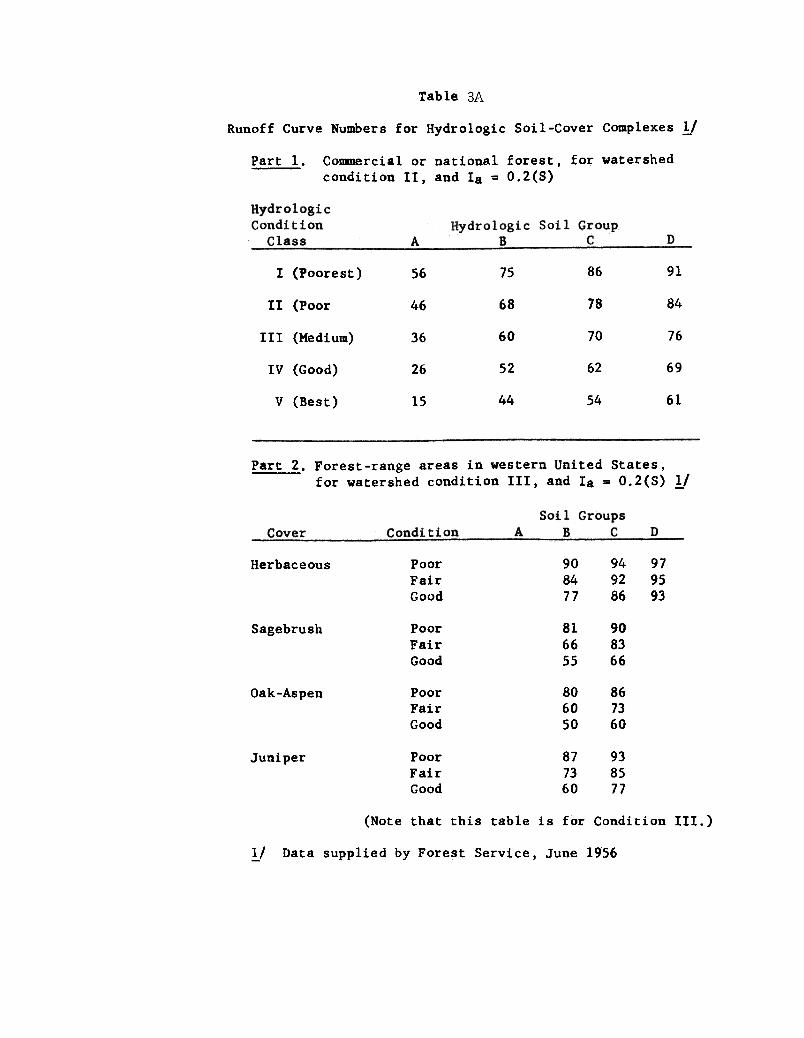
Table 3A

Runoff Curve Numbers for Hydrologic Soil-Cover Complexes !/

Commercial or national forest, for watershed

condition II, and la = O.2(S)Part 1.

86 91I (Poorest) 7556

84II (Poor 68 7846

60 70 76III (Medium) 36

52 62 69IV (Good) 26

44 54 61v (Best) 15

Part 2. Forest-range areas in western United States,for watershed condition III. and Ia = 0.2(5) !1

908477

949286

979593

Herbaceous PoorFairGood

Sagebrush PoorFairGood

81

66

55

90

83

66

806050

867360

Oak-Aspen PoorFairGood

877360

938577

Juniper PoorFairGood

(Note that this table is for Condition III.)

1/ Data supplied by Forest Service, June 1956

38.Table

1

Curve numbers (CN) and constants for the case Ia

7) 4 5 1 2 3 4

= 0.2 S

~2

CN f~r CN for S Curve* CN f~r CN for S Curve*

cond~- ..starts cond~- ..startst .cond~t~ons values* h t .con'i~t~ons values*

h~on I III were ~on I III wereII p = II p =

~)

78

77

76

7.'5

7.'5

74

73

72

71

70

70

69

68

67

66

6.'5

64

63

62

61

60

.'59

.'58

.'57

.'56

.'5.'5

.'54

.'53

.'52

.'51

.'50

6.6.7.7.7.8.8.8.9.9.

10.10.10.11.11.12.12.13.13.14.15.15.16.17.17.18.19.20.21.22.23.

60595857565554535251504948474645444342414039383736353433323130

40393837363534333231313029282726252524232221212019181817161615

10099989796959493929190898887868584838281eo79787776757473727170696867666564636261

100loo9999999898ge9797969695959494939392929191908989888887868685848483828281807978

0 0 1.331.391.451.511.571.641.701.771.851.922.002.082.162.262.342.442.542.642.762.883.003.123.263.403.563.723.884.064.244.444.66

1009794918Q87858381eo787675737270686766646362605958575554535251504847464544434241

.101

.204

.309

.417

.526

.638

.753

.870

.9891.ll1.241.361.491.631.761.902.052.202.342.502.662.822.993.163.333.513.703.894.084.284.494.704.925.155.385.625.876.136.39

.02

.04

.06

.08

.ll

.13

.15

.17

.20

.22

.25

.27

.30

.33

.35

.38

.41

.44

.47

.50

.53

.56

.60

.63

.67

.70

.74

.78

.82

.86

.90

.94

.981.031.081.121.171.231.28

2520151050

12

9642O

43 30.0 6.00

37 40.0 8.00

30 56.7 11.3422 90.0 18.00

13 190.0 38.000 inf'ini ty inf'ini ty

*For CI:1 in column 1.

,67

,95,24

,54,86

,18

,52

,87

,23,61

,0

,4

,8

,3

,7,2

.7

.2

.8

,4

.0

.6

.3

.0

.8

.6

.4

.3

.2

.2

.3

TABLE 4

Table 4- Hydrograph families and To/Tp ratios for which dimension-

less hydrograph ratios are given in Table 5.

TO/Tp

10Hydrograph

Family 36 50 75252 4 161 1.5 3 6

* 7(* * .,.(*1 * * ;': * * *

* * * ** *,'I' * ** * *

* * ** * ** *3 ,... 'I'.. ~.( *

* * * * **4 * * .,.~ * *

* * * ** *5 * .,.( * * *

Asterisks signify that dUnensionless hydrograph tabulations are given

in Table 5.

Table 5 -Time and dischl:!rge ratios for dimensionless hydro graphs

Sheet 1 of 15Hydro graph f8Jnily 1

I"TJTp

3ToiTp =To/Tp = 1.5 = 2T IT = 1o p

Line l t/Tp

No.

LineNo. t/TpLine

No.LineNo.

qc/qp qc/qp