1

MODIS- and AVHRR-derived Polar Winds Experiments using the NCEP GDAS/GFS

NA10NES4400011

Final Report

June 2010 to May 2014

27 August 2014

David Santek, PI Proposed Work Atmospheric Motion Vectors (AMV) are routinely generated from geostationary and polar orbiting satellites and incorporated into most global numerical weather prediction models throughout the world. However, advances in the AMV derivation process and changes to assimilation systems and forecast models require continual reevaluation of the strategies for assimilating satellite-derived winds. The focus of the proposal was in three areas, using AMVs generated from polar orbiting satellite data:

1. Quality control (QC) and thinning using the Expected Error (EE) 2. Experiments assimilating polar winds derived from Advanced Very High

Resolution Radiometer (AVHRR) images; and, 3. Experiments designed to simulate winds from the Visible/Infrared

Imager/Radiometer Suite (VIIRS) instrument onboard the future NPOESS Preparatory Project (NPP) and National Polar-Orbiting Operational Environmental Satellite System (NPOESS) satellites [now restructured as the Joint Polar Satellite System (JPSS)].

The anticipated result of the above experiments is a new QC method for polar winds based on the EE for use in the GDAS/GFS. The design would enable a more easily tunable QC setting for future datasets compared to the current QC technique, making it applicable to the existing MODIS, upcoming AVHRR, and future VIIRS polar winds products. Necessary code changes to the GSI would be transitioned into NCEP operations. Summary of Accomplishments The first two years of the project were spent running experiments in the GDAS/GFS using the EE with the MODIS polar winds. The forecast impact compared to the control was slightly improved, especially in situations where the control performed poorly. Despite these encouraging results with the MODIS winds, the use of the EE for quality control was abandoned when:

• An analysis of the polar winds EE did not correlate with AMV quality, unlike the geostationary EE values.

• There did not appear to be plan within NESDIS to update the EE regression coefficients for AVHRR and VIIRS, instead the coefficients from MODIS were to be used.

2

For the remainder of the project, our new QC was focused on a technique Li Bi applied to OSCAT winds that had favorable results: a threshold based on the speed normalized Observation minus Background (OmB) vector difference. We modified this slightly to normalize by the log of the speed, due to the large range in AMV speed: the Log Normalized Vector Departure (LNVD). The LNVD has similar characteristics as using the EE, in that more slow-speed winds are discarded and more high-speed winds are retained as compared to the control. The forecast impact using the LNVD tended to be neutral to statistically positive for the MODIS winds and neutral for AVHRR-only experiments. Since this project was extended one year, we were able to complete two seasons of MODIS and one season of AVHRR experiments using the LNVD. However, no evaluation of VIIRS AMVs was possible since the routine generation of the AMVs did not begin until May 2014. As proposed:

• a new QC technique (LNVD) was developed for use with satellite-derived polar AMVs that is more easily configurable than the current method in the operational GSI,

• the forecast impact is neutral to slightly positive using MODIS and AVHRR AMVs, and

• the GSI code changes have been checked in for eventual transition into the operational code.

Project Details The following sections summarize the significant experiments that were run, analysis of results, technical issues encountered, personnel, and a list of conference presentations. Additional details can be found in the individual semi-annual reports submitted. The three main experiments are the EE Threshold, EE Ratio, and the LNVD. Expected Error Threshold Experiments Although the Expected Error (EE) was not chosen as the basis for the new quality control technique, the exercise did provide a valuable analysis of the current QC method and how the EE threshold differed in terms of accepted and rejected AMVs. The current operational quality control system for satellite-derived MODIS winds is based on a set of three criteria; a wind observation is rejected if:

1. The pressure level of the observation is within 50 hPa of the tropopause. 2. The difference between the observed and background zonal or meridional flow is

greater than a threshold value (qcU=qcV=7 ms-1)1. 3. The observation is within 200 hPa of the surface and appears over land or ice.

While criteria (1) and (3) are practical considerations concerning the trustworthiness of satellite-derived wind observations near the tropopause or the Earth’s surface, criterion 1 qcU = qcV = (ObsSpd + 15)/3 (IR wind within 200 hPa of surface OR WV wind below 400 hPa) AND (GuessSpd +15)/3 < qcU

3

(2) is meant only to reject observations when they disagree with the model background by more than a fixed amount. The Expected Error is a measure of wind speed error that is derived from a regression using traditional Quality Indicators (QI) which compare characteristics of observations to each other and to the operational forecast, wind speed, and wind and temperature shear that constitute a measure of the synoptic-scale environment. The Expected Error is mostly decoupled from the wind speed OmB and serves as a measure of error that is more independent from the potential innovation than the OmB metric. A control and EE threshold experiment was run using the MODIS AMVs for 24 August – 01 October 2010. A first attempt was made to find a suitable threshold of Expected Error that can replace criterion (2), while leaving the other QC criteria in place. We used an Australian Bureau of Meteorology recommended value of eliminating winds where the EE > 5 ms-1. In order to retain higher speed winds that are usually assigned a high EE value, we additionally required the EE to be larger than 0.1*speed before discarding. Therefore, criterion (2) becomes:

2. The EE is greater than 5 ms-1 and the EE is greater than 10% of the observed wind speed.

Differences between the two model runs in terms of accepted observations were examined over a 10-day period: 10-19 September 2010. There were 2.5 million vectors; in the control 800,000 were accepted, while in the experiment only 200,000 passed the EE threshold criteria. However, the OmB and Observation minus Analysis (OmA) were very similar for the control and experiment for the u- and v-components (Table 1 and Table 2) Table 1: U-component OmB and OmA statistics of the control and EE experiment for 10-19 September 2010. All quantities are in ms-1.

Control (Mean)

Control (StdDev)

EE experiment (Mean)

EE experiment (StdDev)

OmB -0.1 2.5 -0.1 2.2 OmA 0.0 2.2 0.0 1.9

Table 2: V-component OmB and OmA statistics of the control and EE experiment for 10-19 September 2010.

Control (Mean)

Control (StdDev)

EE experiment (Mean)

EE experiment (StdDev)

OmB -0.1 2.6 -0.1 2.3 OmA 0.0 2.2 0.0 1.9

These results were encouraging since using the EE provides a more quantitative screening of the data, whereas the operational quality control method discarded polar wind observations if either the u- or v- component deviated from the background by more than 7 ms-1. The relationship between wind speed OmB and the Expected Error is not particularly strong, but conforms to expectations with low OmB values correlated to low Expected Error (Figure 1).

4

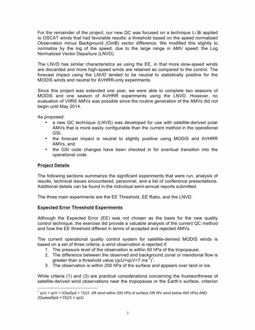
Figure 1: Scatter plot of OmB wind speed (ordinate) and Expected Error (abscissa) of MODIS AMVs for 0000 UTC 21 September 2010. Red (blue) points are rejected (accepted) observations in the (a) experiment and (b) control.

While low EE typically translates to low OmB wind speed, the reverse is not necessarily true; a high EE can have an incredibly wide variance in OmB wind speed. Provided that the EE can be thought of as a measure of wind speed error largely independent of OmB wind speed, Figure 1 illustrates that a low OmB wind speed does not ensure that an observation should be trusted. While the operational QC procedure (Figure 1b) removed very few observations near the OmB > 7 ms-1 threshold, the new EE threshold (Figure 1a) drastically reduces the number of accepted observations to only those with a low EE. Our expectation is that these modifications to polar winds will have a largely neutral impact on anomaly correlation (AC) scores computed globally or over a hemisphere, except for mid-range (5-7 day) forecasts in which polar or near-polar features play an important role. As such, we expect impact from these modifications to only be reflected in certain Day-5 to Day-7 forecasts, and remain neutral otherwise. It is also expected that these modifications will have a greater impact in the southern hemisphere, where satellite winds typically have a larger impact on the analysis. A time-series of Day-5 AC scores reveals similar characteristics (Figure 2).

5

Figure 2: Day-5 anomaly correlation scores for 24 forecasts between 08 September 2010 and 01 October 2010. Scores are computed for 500 hPa geopotential heights over the southern hemisphere (20ºS-80ºS) for the control (black) and the experiment (red).

For the month of September 2010, the only significant impact occurs on the 26th, when the control simulation nearly busts with a Day-5 AC value of almost 0.7, while the experiment sees significant improvement. It is interesting to note that an even worse forecast is made for 01 October, though the experiment and control are practically identical. Both the 26 September and 01 October events are poorly forecast by the control run, while the EE experiment appears to improve only the 26 September event. One can assume that the discrepancy between these two events can be traced back to one or both of the following:

1. Differences in the synoptic evolution of both forecasts that allows for communication of improved initial conditions at polar latitudes to impact one event but not the other.

2. Differences in the amount of information provided by MODIS wind observations in the initial conditions of both forecasts.

Expected Error Ratio Experiments The operational QC and EE threshold experiments resulted in many of the high-speed winds being thinned. This was considered a possible reason that the impact of the MODIS winds is generally neutral. While the satellite sounder radiances provide much information on atmospheric structure in regions that are clear, the impact of the MODIS winds can complement by providing information in highly dynamic, cloudy regions of the troposphere. The following experiment is designed to evaluate these previously discarded winds using a new QC method: EE Ratio. The EE Ratio experiment eliminates MODIS AMVs if the EE Ratio (defined as EE/observation_speed) is less than a specified threshold. The threshold used was 1.3367, which was empirically determined to result in approximately the same number of rejections as the control. Over the six-week period, 3 million observations were accepted; 250,000 rejected. However, the experiment accepted about 36,000 (1%) more observations than the control.

6

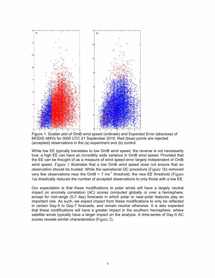
Figure 3 is a density plot of the normalized background speed departure vs. EE Ratio for the MODIS IR winds in January 2012. The three curves represent the mean normalized speed departure (middle) and +/- one standard deviation. Since the standard deviation decreases with smaller EE Ratio (the lines converge from right to left), the EE Ratio does show some skill in reducing the spread of the normalized OmB distribution. Therefore, this is a reasonable candidate for QC screening.

Figure 3: Normalized background speed departure vs. EE Ratio for the MODIS IR winds in January 2012 for the northern hemisphere (top) and southern hemisphere (bottom). The three curves represent the mean normalized speed departure (middle) and +/- one standard deviation.

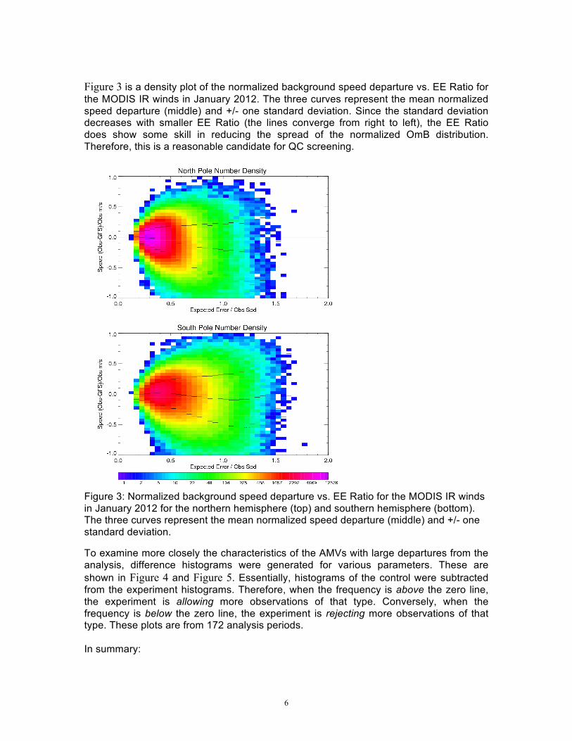
To examine more closely the characteristics of the AMVs with large departures from the analysis, difference histograms were generated for various parameters. These are shown in Figure 4 and Figure 5. Essentially, histograms of the control were subtracted from the experiment histograms. Therefore, when the frequency is above the zero line, the experiment is allowing more observations of that type. Conversely, when the frequency is below the zero line, the experiment is rejecting more observations of that type. These plots are from 172 analysis periods. In summary:

7

• More winds are retained with EE > 5 ms-1 (Figure 4 left). We had used this threshold in previous experiments, which resulted in a very neutral impact.

• More winds are retained in the 250-450 hPa layer (Figure 4 right). These are at the level of the polar jet.

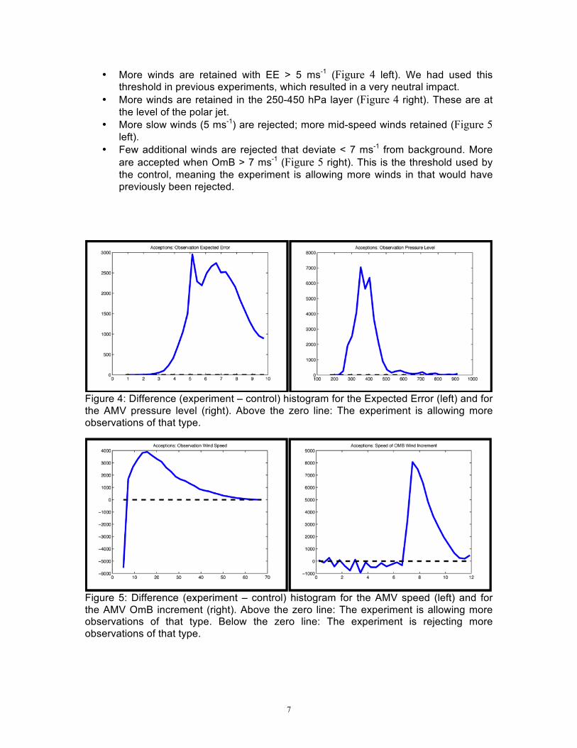
• More slow winds (5 ms-1) are rejected; more mid-speed winds retained (Figure 5 left).

• Few additional winds are rejected that deviate < 7 ms-1 from background. More are accepted when OmB > 7 ms-1 (Figure 5 right). This is the threshold used by the control, meaning the experiment is allowing more winds in that would have previously been rejected.

Figure 4: Difference (experiment – control) histogram for the Expected Error (left) and for the AMV pressure level (right). Above the zero line: The experiment is allowing more observations of that type.

Figure 5: Difference (experiment – control) histogram for the AMV speed (left) and for the AMV OmB increment (right). Above the zero line: The experiment is allowing more observations of that type. Below the zero line: The experiment is rejecting more observations of that type.

8

Based on the above analysis, the selection of an EE Ratio threshold based on a similar number of rejections as the control, results in accepting more higher speed winds at the jet level, while rejecting more slow winds. Also, these additionally accepted winds deviate more from the background than the operational QC would allow. However, since the additional winds are small in number, OmB and OmA statistics remain the same. The following discusses the forecast impact. Figure 6 and Figure 7 show forecast impact of this new QC method compared to the control as measured by the hemispheric Anomaly Correlation (AC) at 500 hPa. The averaged AC score (left panels of Figure 6 and Figure 7) is for 35 days from mid-January to late-February 2012. The daily scores are in the right panels for Day-5, -6, and -7 forecasts. The averaged scores for the northern hemisphere (Figure 6) are neutral for this time period. However, there is a substantial improvement in dropout events near day 30 (circled in Figure 6 right panels), where the experiment (red) out-performed the control (blue).

Figure 6: Anomaly Correlation (AC) scores averaged over five weeks (left) and the daily scores for Day-5, -6, and -7 (right). Date: mid-January to late-February 2012. Scores are computed for 500 hPa geopotential heights over the northern hemisphere (20ºN-80ºN) for the control (blue) and the experiment (red), using the EE Ratio. Improvements in selected dropout events are circled.

Similarly, the averaged scores for the southern hemisphere (Figure 7) are generally neutral, although by Day-7 and -8 the experiment is out-performing the control. Again, there is a substantial improvement in dropout events, this time near day 17 and 18 (circled in Figure 7 right panels), where the experiment (red) out-performed the control (blue).

9

Figure 7: Same as Figure 6, except for the southern hemisphere.

See the December 2012 JCSDA newsletter article, Polar Atmospheric Winds and Forecast Busts, for a discussion on the dropout improvements (or lack thereof) as related to different flow regimes. Expected Error issues When the proposal was written, the Expected Error correlated well with improved OmB statistics for geostationary winds. We expected a similar relationship would follow for the polar winds. However, that does not appear to be the case for the following reasons:

• We did an analysis of both polar and geostationary satellite winds using several weeks of observations, to determine if there is a correlation between winds-related parameters and the EE. For the geostationary winds, the majority of the variance in the correlation is explained by the QI (without forecast), wind speed, and background departure (OmB). Higher quality EE values are associated with higher QI, lower wind speed, and lower OmB. However for the polar winds, the better EE values are correlated with lower wind speed and higher pressure. Unlike the geostationary winds, no measure of quality (e.g., QI or OmB) correlates with the EE for polar winds.

• The EE regression coefficients, derived from a multi-variable regression with RAOBs, vary widely in value between different satellites (Aqua and Terra) and hemisphere (northern and southern). This is unexpected since the MODIS instrument is well calibrated and the performance is very similar between the two satellites. We suspect there is a sampling issue due to very few RAOBs being available for determining the coefficients.

Three other factors contributed to our abandoning the Expected Error:

• Our inspection of the BUFR files containing AVHRR winds did not reveal an EE value. Emails to Xiujuan Su, Jim Jung, Jaime Daniels, and Dennis Keyser could not resolve the issue of why the EE apparently was not contained in the files. It

10

was also learned that if the EE was present, it would be based on the MODIS EE regression coefficients.

• One of the terms in the calculation of the EE is the AMV Quality Indicator (QI) that is dependent on the forecast. From a data assimilation point of view, the AMVs and associated quality information should be independent of the model.

• When the VIIRS winds are first available, it is unlikely there will be an EE associated with the AMVs. If there is, it will be using the coefficients from MODIS. Also, based on the earlier arguments, it will be difficult to compute reliable EE coefficients for VIIRS due to the scarcity of RAOBs.

New quality control: LNVD Discussions with Jim Jung and Li Bi about her encouraging results using a normalized OmB vector difference for OSCAT winds motivated our investigating a similar measure for quality control for the polar winds. However, recognizing that wind speed has a range that covers three orders of magnitude (1, 10, 100 ms-1), we elected to normalize the vector departure by the logarithm of the observation speed. The Log Normalized Vector Departure (LNVD) is defined as:

SQRT ( (Uo-Ub)2 + ( Vo – Vb)2 ) / log(ObsSpd) where Uo, Vo is the observed u- and v- components; Ub, Vb is the background; ObsSpd is the AMV speed. For the initial evaluation of the LNVD, we determined a threshold that would result in the same number of discarded winds as the control and EE ratio experiment. A LNVD threshold of 3 is equivalent to EE ratio of 1.33, and the LNVD has a similar effect as the EE ratio by discarding more slower-speed winds and retaining more higher-speed winds. The operational screening discards AMVs if the u- or v- component differs by more than 7 ms-1 from the background. Therefore, most slow winds (< 5 ms-1) are retained in the control because they will not exceed the 7 ms-1 threshold, even though they may be pointed in the opposite direction! Table 3 shows the allowable AMV departure from the background will vary using a LNVD threshold. Slow winds (speed < 3 ms-1) must be within 3.3 ms-1 to be accepted. On the other end of the scale, a 50 ms-1 wind may deviate from the background by 11.7 ms-1 and still be retained. Table 3: Allowed vector departure from the background (VecDiff) that an AMV will be accepted for sample observations speeds (ObsSpd). The VecDiff increases with increasing wind speed, unlike the operational QC which is fixed at 7 ms-1.

LNVD threshold = 3 ObsSpd Log(ObsSpd) VecDiff

3 1.1 3.3 10 2.3 6.9 50 3.9 11.7

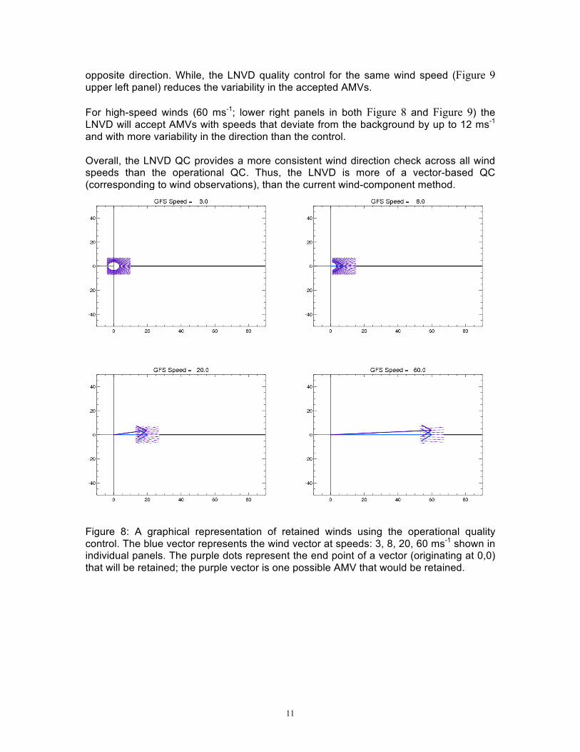
100 4.6 13.8 A graphical depiction of the operational screening (Figure 8) shows that slow winds (upper left panel) can vary substantially from the background, including pointing in the

11

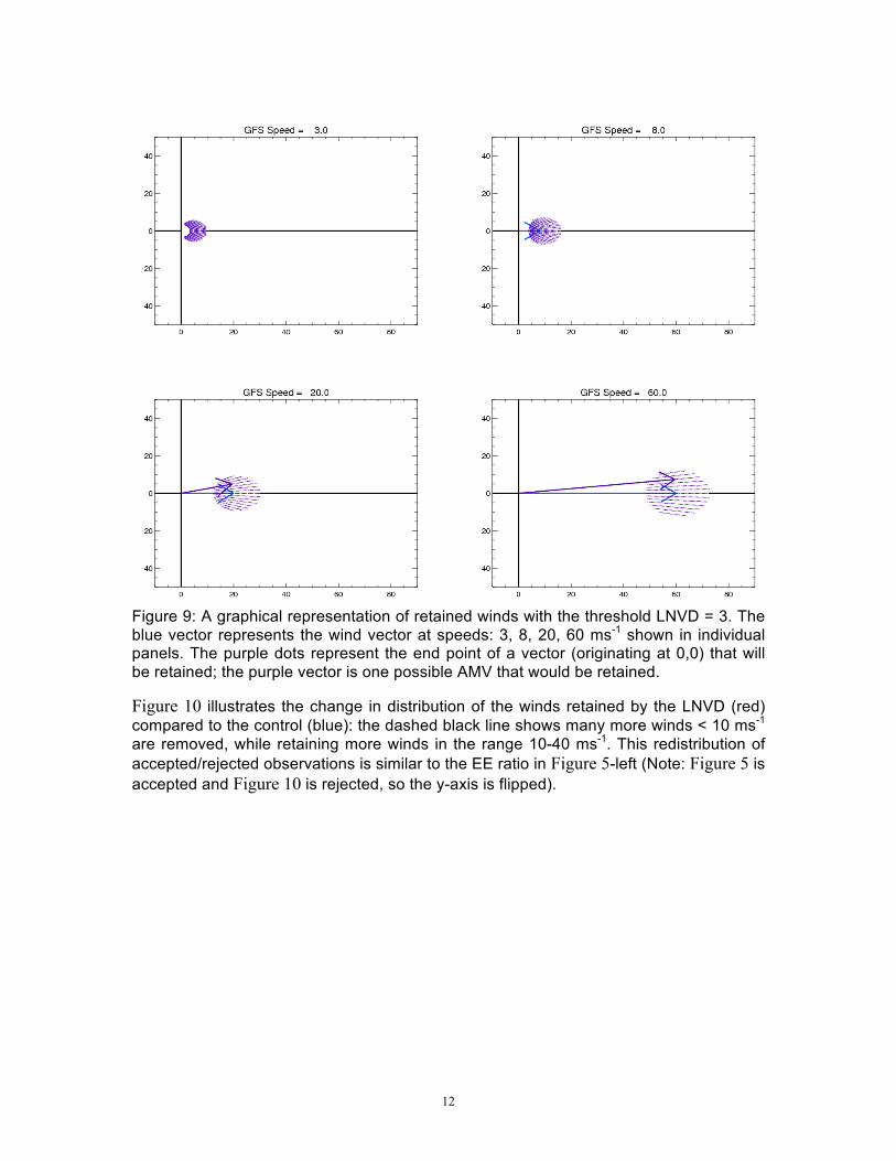
opposite direction. While, the LNVD quality control for the same wind speed (Figure 9 upper left panel) reduces the variability in the accepted AMVs. For high-speed winds (60 ms-1; lower right panels in both Figure 8 and Figure 9) the LNVD will accept AMVs with speeds that deviate from the background by up to 12 ms-1 and with more variability in the direction than the control. Overall, the LNVD QC provides a more consistent wind direction check across all wind speeds than the operational QC. Thus, the LNVD is more of a vector-based QC (corresponding to wind observations), than the current wind-component method.

Figure 8: A graphical representation of retained winds using the operational quality control. The blue vector represents the wind vector at speeds: 3, 8, 20, 60 ms-1 shown in individual panels. The purple dots represent the end point of a vector (originating at 0,0) that will be retained; the purple vector is one possible AMV that would be retained.

Allowable wind departure for AMV from GFS for 4 GFS wind speedsBlue arrows represent GFS wind vector. Purple dots show possible AMV vectors allowed by check. One purple AMV vector is drawn.Component Check

12

Figure 9: A graphical representation of retained winds with the threshold LNVD = 3. The blue vector represents the wind vector at speeds: 3, 8, 20, 60 ms-1 shown in individual panels. The purple dots represent the end point of a vector (originating at 0,0) that will be retained; the purple vector is one possible AMV that would be retained.

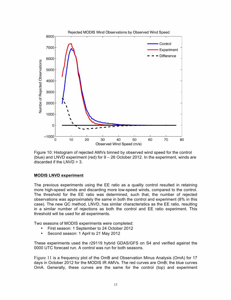
Figure 10 illustrates the change in distribution of the winds retained by the LNVD (red) compared to the control (blue): the dashed black line shows many more winds < 10 ms-1 are removed, while retaining more winds in the range 10-40 ms-1. This redistribution of accepted/rejected observations is similar to the EE ratio in Figure 5-left (Note: Figure 5 is accepted and Figure 10 is rejected, so the y-axis is flipped).

Allowable wind departure for AMV from GFS for 4 GFS wind speedsBlue arrows represent GFS wind vector. Purple dots show possible AMV vectors allowed by check. One purple AMV vector is drawn.Log Normal Vector Check Sqrt[ (Uamv – U gfs)^2 + (Vamv – Vgfs)^2 ] / Log(Speed gfs) < 3

13

Figure 10: Histogram of rejected AMVs binned by observed wind speed for the control (blue) and LNVD experiment (red) for 9 – 26 October 2012. In the experiment, winds are discarded if the LNVD > 3.

MODIS LNVD experiment The previous experiments using the EE ratio as a quality control resulted in retaining more high-speed winds and discarding more low-speed winds, compared to the control. The threshold for the EE ratio was determined, such that, the number of rejected observations was approximately the same in both the control and experiment (8% in this case). The new QC method, LNVD, has similar characteristics as the EE ratio, resulting in a similar number of rejections as both the control and EE ratio experiment. This threshold will be used for all experiments. Two seasons of MODIS experiments were completed:

• First season: 1 September to 24 October 2012 • Second season: 1 April to 21 May 2012

These experiments used the r29119 hybrid GDAS/GFS on S4 and verified against the 0000 UTC forecast run. A control was run for both seasons. Figure 11 is a frequency plot of the OmB and Observation Minus Analysis (OmA) for 17 days in October 2012 for the MODIS IR AMVs. The red curves are OmB; the blue curves OmA. Generally, these curves are the same for the control (top) and experiment

14

(bottom): the bias is nearly zero and the standard deviation is the same. The experiment OmB standard deviation is 2.44 ms-1, which reduces to 2.10 ms-1 for OmA (i.e., the observations have an impact on the analysis). Even though the LNVD method retains winds with a larger background departure, they are few in number so the bulk statistics are very similar to the control.

Figure 11: MODIS IR AMVs Observation Minus Background (OmB) and Observation Minus Analysis (OmA) distributions for 9 – 26 October 2012. The top panels are the control; the lower panels the experiment, for the u-component (left side) and v-component (right side) of the wind.

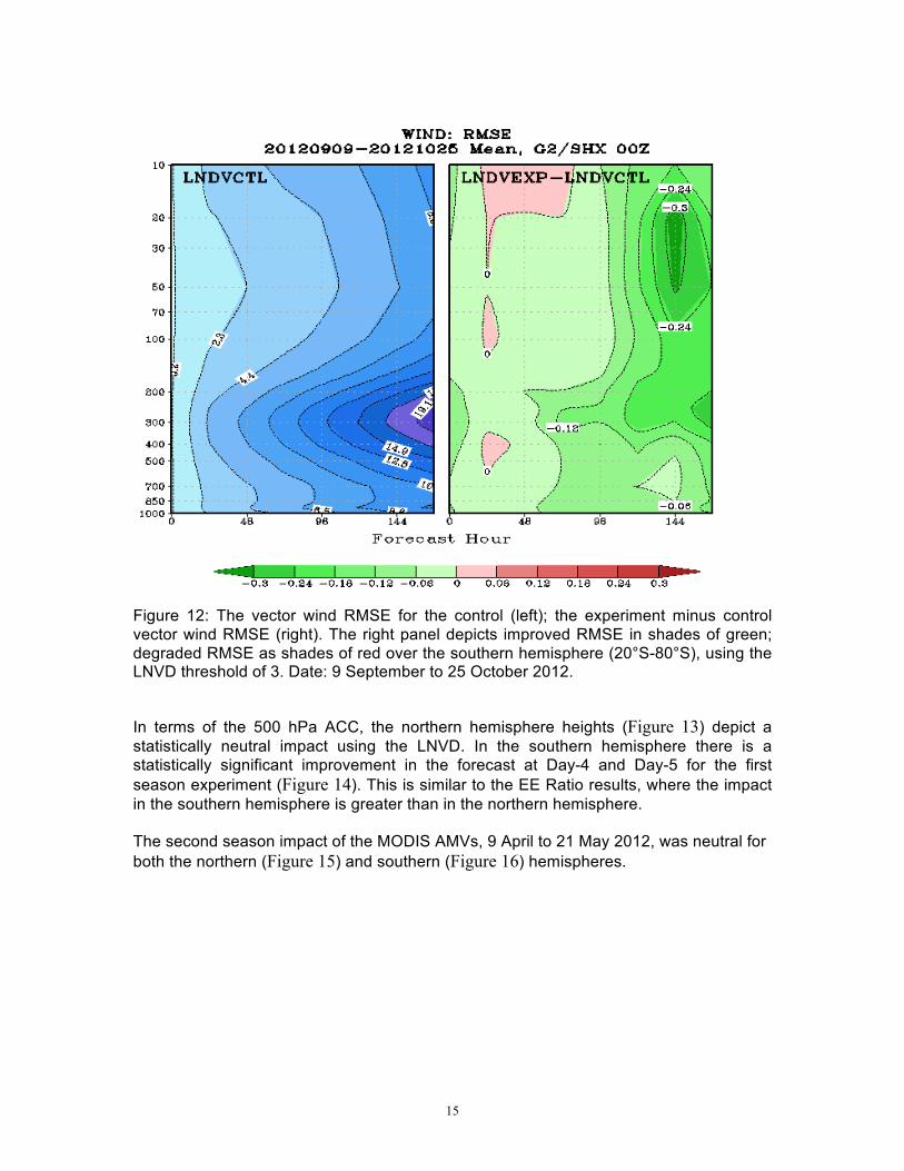
Generally the impact of the LNVD is statistically neutral as compared to the control, although slight improvements are noted. For example, the vertical profile of the southern hemisphere wind RMSE (Figure 12) shows a reduction in the RMSE (right panel) using the LNVD vs. the control. The improvement is centered at the 300 hPa level beginning at about the 48-hour forecast and extending to later forecast times.

15

Figure 12: The vector wind RMSE for the control (left); the experiment minus control vector wind RMSE (right). The right panel depicts improved RMSE in shades of green; degraded RMSE as shades of red over the southern hemisphere (20°S-80°S), using the LNVD threshold of 3. Date: 9 September to 25 October 2012.

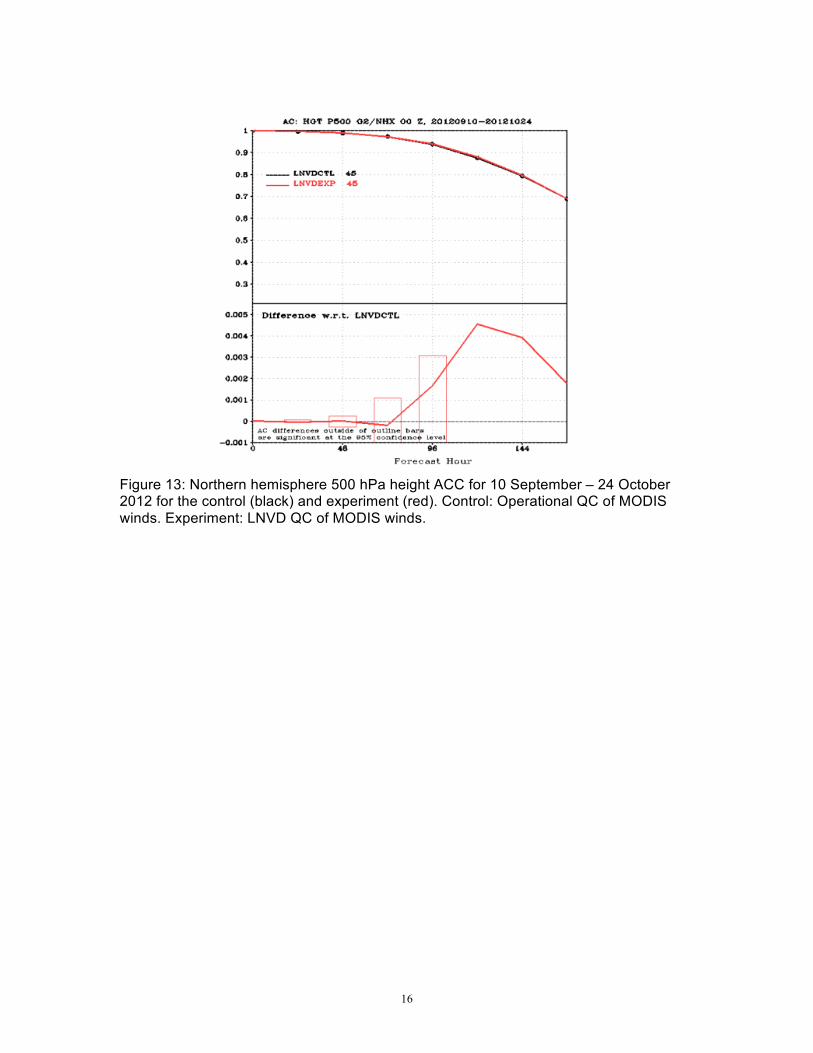
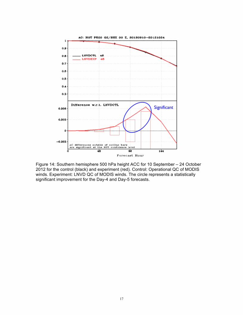
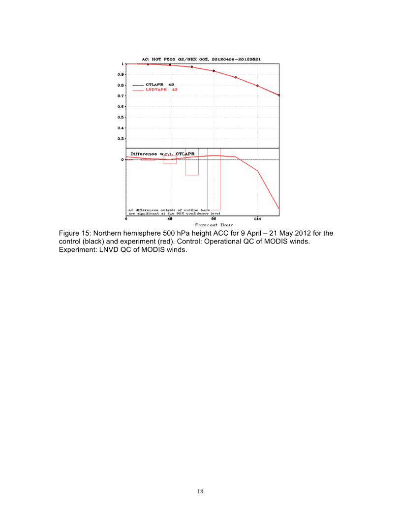
In terms of the 500 hPa ACC, the northern hemisphere heights (Figure 13) depict a statistically neutral impact using the LNVD. In the southern hemisphere there is a statistically significant improvement in the forecast at Day-4 and Day-5 for the first season experiment (Figure 14). This is similar to the EE Ratio results, where the impact in the southern hemisphere is greater than in the northern hemisphere. The second season impact of the MODIS AMVs, 9 April to 21 May 2012, was neutral for both the northern (Figure 15) and southern (Figure 16) hemispheres.

16

Figure 13: Northern hemisphere 500 hPa height ACC for 10 September – 24 October 2012 for the control (black) and experiment (red). Control: Operational QC of MODIS winds. Experiment: LNVD QC of MODIS winds.

17

Figure 14: Southern hemisphere 500 hPa height ACC for 10 September – 24 October 2012 for the control (black) and experiment (red). Control: Operational QC of MODIS winds. Experiment: LNVD QC of MODIS winds. The circle represents a statistically significant improvement for the Day-4 and Day-5 forecasts.

Significant

18

Figure 15: Northern hemisphere 500 hPa height ACC for 9 April – 21 May 2012 for the control (black) and experiment (red). Control: Operational QC of MODIS winds. Experiment: LNVD QC of MODIS winds.

19

Figure 16: Southern hemisphere 500 hPa height ACC for 9 April – 21 May 2012 for the control (black) and experiment (red). Control: Operational QC of MODIS winds. Experiment: LNVD QC of MODIS winds.

AVHRR LNVD experiment A single season experiment was completed using AVHRR IR winds with the same LNVD settings as MODIS. The real-time AVHRR winds are from NOAA-15, -16, -18, -19, and Metop-A for this time period. For the NOAA satellites, features are tracked in 4 km resolution images (compared to 2 km for MODIS). However, for the Metop satellite the resolution is the same as MODIS. This results in more AVHRR IR winds as compared to MODIS, but MODIS has a substantial contribution from water vapor winds. However, Terra water vapor winds are no longer being produced by NESDIS since there are only two good detectors out of ten for band 27 (6.7 µm). In this experiment, the AVHRR winds replace the MODIS winds and the statistics presented are compared to their respective background and analysis. This scenario is important as the MODIS instruments on Terra and Aqua are well beyond their designed lifetimes, so AVHRR-only polar winds may be a reality in the near future. This experiment compares the impact of the MODIS winds with operational quality control (Control) and AVHRR winds (Experiment) with the LNVD. The impact is statistically neutral for both the northern (not shown) and southern hemispheres (Figure 17) However, the result is encouraging as AVHRR (and VIIRS) polar winds will be the replacement product for MODIS as it operates beyond its designed lifetime.

20

Figure 17: Southern hemisphere 500 hPa height ACC for 10 September – 13 October 2012 for the control (black) and experiment (red). Control: Operational QC of MODIS winds. Experiment: LNVD QC with AVHRR winds (no MODIS winds).

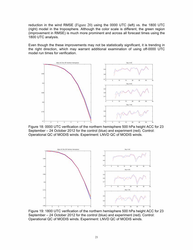
1800 UTC Model Run for Verification The forecast impact is typically measured using the 0000 UTC model run, which contains the most input data. Would satellite-derived polar AMVs have a more significant forecast impact if it were measured at a time when radiosondes were not available? The following is a comparison of the impact of the MODIS winds using the 0000 UTC and 1800 UTC forecast run. This is for a one-month period of the LNVD experiment: 23 September - 24 October 2012. Figure 18 depicts the northern hemisphere 500 hPa height ACC dieoff curves (left) and the daily scores (right) for the control (blue) and MODIS LNVD experiment (red). The impact is neutral out to Day-5, and then the control is slightly better than the experiment out to Day-7. Note: There are dropouts early in the run (Day-7 ACC in lower-right) with a mostly neutral impact the remainder of the time period. Using the 1800 UTC model run as verification also shows a generally neutral impact (Figure 19), however in the later forecast times the experiment is slightly better. This is the opposite of what was observed for the 0000 UTC verification. Additionally, there is a

21

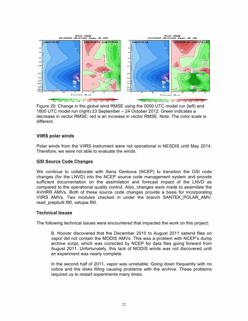
reduction in the wind RMSE (Figure 20) using the 0000 UTC (left) vs. the 1800 UTC (right) model in the troposphere. Although the color scale is different, the green region (improvement in RMSE) is much more prominent and across all forecast times using the 1800 UTC analysis. Even though the these improvements may not be statistically significant, it is trending in the right direction, which may warrant additional examination of using off-0000 UTC model run times for verification.

Figure 18: 0000 UTC verification of the northern hemisphere 500 hPa height ACC for 23 September – 24 October 2012 for the control (blue) and experiment (red). Control: Operational QC of MODIS winds. Experiment: LNVD QC of MODIS winds.

Figure 19: 1800 UTC verification of the northern hemisphere 500 hPa height ACC for 23 September – 24 October 2012 for the control (blue) and experiment (red). Control: Operational QC of MODIS winds. Experiment: LNVD QC of MODIS winds.

1 2 3 4 5 6 7 80.7

0.75

0.8

0.85

0.9

0.95

1Mean AC Die−Off: Northern Hemisphere

0 5 10 15 20 25 30 350.7

0.8

0.9

1Day−5 AC

0 5 10 15 20 25 30 35

0.7

0.8

0.9

1Day−6 AC

0 5 10 15 20 25 30 350.4

0.6

0.8

1Day−7 AC

1 2 3 4 5 6 7 80.65

0.7

0.75

0.8

0.85

0.9

0.95

1Mean AC Die−Off: Northern Hemisphere

0 5 10 15 20 25 30 350.7

0.8

0.9

1Day−5 AC

0 5 10 15 20 25 30 35

0.7

0.8

0.9

1Day−6 AC

0 5 10 15 20 25 30 350.4

0.6

0.8

1Day−7 AC

22

Figure 20: Change in the global wind RMSE using the 0000 UTC model run (left) and 1800 UTC model run (right) 23 September – 24 October 2012. Green indicates a decrease in vector RMSE; red is an increase in vector RMSE. Note: The color scale is different.

VIIRS polar winds Polar winds from the VIIRS instrument were not operational in NESDIS until May 2014. Therefore, we were not able to evaluate the winds. GSI Source Code Changes We continue to collaborate with Iliana Genkova (NCEP) to transition the GSI code changes (for the LNVD) into the NCEP source code management system and provide sufficient documentation on the assimilation and forecast impact of the LNVD as compared to the operational quality control. Also, changes were made to assimilate the AVHRR AMVs. Both of these source code changes provide a basis for incorporating VIIRS AMVs. Two modules checked in under the branch SANTEK_POLAR_AMV: read_prepbufr.f90, setupw.f90. Technical Issues The following technical issues were encountered that impacted the work on this project:

B. Hoover discovered that the December 2010 to August 2011 satwnd files on vapor did not contain the MODIS AMVs. This was a problem with NCEP’s dump archive script, which was corrected by NCEP for data files going forward from August 2011. Unfortunately, this lack of MODIS winds was not discovered until an experiment was nearly complete. In the second half of 2011, vapor was unreliable: Going down frequently with no notice and the disks filling causing problems with the archive. These problems required us to restart experiments many times.

23

Access to vapor ended in mid-March 2012. A request was sent to Jim Yoe in January 2012 to delay the decommissioning of vapor until June 2012, in anticipation that S4 would be available by then. This request was denied. We decided not to pursue running experiments on zeus for the following reasons:

• The eventual goal is to run on S4; moving to zeus for just a few months did not seem worth the effort (moving data, updating code, modifying scripts, learning new procedures).

• The reliability and stability of zeus did not appear to be very good during the time following the decommissioning of vapor.

• There was enough work to do in preparation for using S4. S4 was not available until August 2012, about 5 months after vapor was decommissioned.

NESDIS operations began sending AVHRR polar winds to NCEP in 2011. However, this dataset did not include the EE nor did it span the day boundary. We anticipated that these two issues would be resolved in the first quarter of 2012. Unfortunately, the former issue was not complete until the last week in June 2012. Spanning the day boundary is very important in determining the impact of the winds, since it’s typically the 00 UTC run where the full forecast is run and statistics computed. This delayed running AVHRR experiments until the latter half of 2012.

A first season experiment (Fall 2012) running the hybrid GDAS/GFS was designed to include Hurricane Sandy. However, we were not able to run past 25 October 2012 on S4 due to an issue in2:

“…the prep step when hurricane relocation is done. Somehow bad sfcP obs are getting into the relocation and show up in the sigges.gdas file that goes into the analysis. The GSI runs fine, but the analysis fields carry the anomaly through. These anomalous fields then crash the GFS code with a seg fault in the long or shortwave IR RT calculations. This appears to only impact people using their own compiled version of GSI on S4.”

Since we compile the GSI on S4 in order to implement the LNVD quality control, our experiments ended on 25 October 2012.

Personnel B. Hoover, S. Nebuda, and D. Santek of CIMSS ran the GDAS/GFS experiments on vapor and S4, and used the Verification Statistics Data Base (VSDB) software to generate statistics and plots. James Jung visited twice to train CIMSS personnel on running the GDAS/GFS on vapor (November 2010) and S4 (January 2012). The training covered customizing the scripts, explanations of procedures, best practices when running experiments, and modifying and building the GSI software. Conferences and Workshops Santek attended the GSI Data Assimilation System Tutorial from 28-30 June 2010 at the NCAR Foothills Laboratory, Boulder, Colorado. 2 Kevin Garrett, personal communication 12 February 2014.

24

http://www.dtcenter.org/com-GSI/users/tutorials/gsi_tutorial_2010.2.php Santek, D. and B. Hoover, 2011. Using the Expected Error in the assimilation of satellite-derived winds Part 1: Quality control impact. 9th JCSDA Workshop on Satellite Data Assimilation, College Park, MD. Hoover, B. and D. Santek, 2011. Using the Expected Error in the assimilation of satellite-derived winds Part 2: Forecast impact. 9th JCSDA Workshop on Satellite Data Assimilation, College Park, MD. Santek, D., B. Hoover, and J. Jung, 2011. Using the Expected Error in the quality control of satellite-derived polar winds. 2011 EUMETSAT Meteorological Satellite Conference. Oslo, Norway. Santek, D., B. Hoover, and J. Jung, 2012. The quality control of satellite-derived polar winds using the Expected Error. 16th Symposium on Integrated Observing and Assimilation Systems for the Atmosphere, Oceans, and Land Surface (IOAS-AOLS), AMS, New Orleans, LA. Santek, D., B. Hoover, and J. Jung, 2012. Assimilation and forecast impacts using the Expected Error in the quality control of MODIS polar winds. 11th International Winds Workshop, Auckland, New Zealand. Santek, D., B. Hoover, J. Jung, and S. Nebuda, 2012. Quality control of MODIS and AVHRR polar winds in the GDAS/GFS: Status and plans. 10th Annual JCSDA Workshop on Satellite Data Assimilation. College Park, MD. Santek, D., B. Hoover, S. Nebuda, and J. Jung, 2013. Status of improving the use of MODIS, AVHRR, and VIIRS polar winds in the GDAS/GFS. 11th Annual JCSDA Workshop on Satellite Data Assimilation. College Park, MD. Hoover, B. and D. Santek, 2012. Polar Winds and Forecast Busts. JCSDA Quarterly. No. 41, December 2012. http://www.jcsda.noaa.gov/documents/newsletters/201212JCSDAQuarterly.pdf Santek, D., B. Hoover, and S. Nebuda, 2014. Evaluation of a new method to quality control satellite-derived polar winds in the NCEP GDAS/GFS. Second Symposium on the Joint Center for Satellite Data Assimilation. AMS, Atlanta, GA. Santek, D., B. Hoover, S. Nebuda, and J. Jung, 2014. Status of improving the use of MODIS and AVHRR polar winds in the GDAS/GFS. 12th JCSDA Technical Review Meeting & Science Workshop on Satellite Data Assimilation. College Park, MD.