nao devils dortmund team report 2011 · nao devils dortmund team report 2011 stefan ... speed yet...
TRANSCRIPT

Nao Devils Dortmund
Team Report 2011
Stefan Tasse, Soren Kerner, Oliver Urbann,
Matthias Hofmann, Ingmar Schwarz
Robotics Research InstituteSection Information Technology
Contents
1 Introduction 11.1 Team Description . . . . . . . . . . . . . . . . . . . . . . . . . . . . . . . . 21.2 Software Overview . . . . . . . . . . . . . . . . . . . . . . . . . . . . . . . 2
2 Motion 42.1 Walking . . . . . . . . . . . . . . . . . . . . . . . . . . . . . . . . . . . . . 4
2.1.1 Dortmund Walking Engine . . . . . . . . . . . . . . . . . . . . . . 52.1.2 The ZMP/IP-Controller . . . . . . . . . . . . . . . . . . . . . . . . 7
Sensor Feedback Sources . . . . . . . . . . . . . . . . . . . . . . . . 7Integration of the Measurements, a Sensor Fusion . . . . . . . . . . 9Experimental Sensor Feedback Methods . . . . . . . . . . . . . . . 10
2.1.3 ZMP Generation . . . . . . . . . . . . . . . . . . . . . . . . . . . . 102.1.4 Swinging Leg Controller . . . . . . . . . . . . . . . . . . . . . . . . 12
2.2 Kicking . . . . . . . . . . . . . . . . . . . . . . . . . . . . . . . . . . . . . 122.3 Special Actions . . . . . . . . . . . . . . . . . . . . . . . . . . . . . . . . . 13
3 Cognition 153.1 Image Processing . . . . . . . . . . . . . . . . . . . . . . . . . . . . . . . . 153.2 Line and Circle Detection . . . . . . . . . . . . . . . . . . . . . . . . . . . 173.3 Localization . . . . . . . . . . . . . . . . . . . . . . . . . . . . . . . . . . . 193.4 Distributed World Modeling . . . . . . . . . . . . . . . . . . . . . . . . . . 203.5 Current Research . . . . . . . . . . . . . . . . . . . . . . . . . . . . . . . . 22
3.5.1 Cooperative EKF-SLAM World Modeling . . . . . . . . . . . . . . 233.5.2 Active Vision . . . . . . . . . . . . . . . . . . . . . . . . . . . . . . 253.5.3 Colortable-less Image Processing . . . . . . . . . . . . . . . . . . . 28
4 Behavior 314.1 Implementation of Collaborating Soccer Agents . . . . . . . . . . . . . . . 334.2 Behavior Coordinate System . . . . . . . . . . . . . . . . . . . . . . . . . 354.3 GoTo Motion Command . . . . . . . . . . . . . . . . . . . . . . . . . . . . 364.4 Debug Tool . . . . . . . . . . . . . . . . . . . . . . . . . . . . . . . . . . . 37
5 Conclusion and Outlook 42
i
A Getting Started 43A.1 Setting up the development environment . . . . . . . . . . . . . . . . . . . 43
A.1.1 Windows . . . . . . . . . . . . . . . . . . . . . . . . . . . . . . . . 43A.1.2 Linux . . . . . . . . . . . . . . . . . . . . . . . . . . . . . . . . . . 45A.1.3 Build configurations . . . . . . . . . . . . . . . . . . . . . . . . . . 45
A.2 Setting up the robot . . . . . . . . . . . . . . . . . . . . . . . . . . . . . . 45A.2.1 Preparing the memory stick . . . . . . . . . . . . . . . . . . . . . . 45A.2.2 Copying your current code and configuration to the robot . . . . . 46A.2.3 Starting and stopping the robot . . . . . . . . . . . . . . . . . . . . 46A.2.4 How to connect with the robot and debug . . . . . . . . . . . . . . 47A.2.5 Using the XABSL Debug Tool . . . . . . . . . . . . . . . . . . . . 47
B Framework 49B.1 Modules . . . . . . . . . . . . . . . . . . . . . . . . . . . . . . . . . . . . . 49B.2 Representations . . . . . . . . . . . . . . . . . . . . . . . . . . . . . . . . . 50B.3 Origin of Modules . . . . . . . . . . . . . . . . . . . . . . . . . . . . . . . 50
C Walking Engine Parameters 55C.1 File walkingParams.cfg . . . . . . . . . . . . . . . . . . . . . . . . . . . . . 55C.2 File NaoNG.m . . . . . . . . . . . . . . . . . . . . . . . . . . . . . . . . . 58
ii

Chapter 1
Introduction
Competitions such as the RoboCup provide a benchmark for the state of the art in thefield of autonomous mobile robots and provide researchers with a standardized setup tocompare their research. Additionally the RoboCup Standard Platform League does notonly provide researchers with a common setup, but also with the same hardware platformto use. This renders increased importance to publications of those teams, since extensivedocumentation and especially releasing source code allows other researchers to compareresults and methods, reuse and improve them, and to further common research goals.
In the course of this report some of the points of the robot software and current theresearch approach of the RoboCup team Nao Devils are described. An overview aboutthe Nao Devils software is given in section 1.2. This software has been used in thecompetitions in 2011 and is also included in the code release that is published along withthis report1. This code release contains the complete code used by team Nao Devils duringthe RoboCup 2011, but the behavior and the tuned walking parameters are replaced bya more basic version. Also contained are the developed tools, out of which the behaviordebug tool is described in detail in section 4.4.
Stable motions are of crucial importance in the context of biped robots. Thus, thefollowing chapter of the document will describe the motion control process emphasizingthe Dortmund Walking Engine which has been the first closed loop walking engine ap-plied to the Nao in RoboCup 2008, 2009 and 2010. The version of RoboCup 2010 wasable to reach walking speeds of up to 44cm/s, which is, to our knowledge, the highestspeed yet achieved with the robot Nao. Incidentally this speed exceeds the “theoreticalmaximum walking speed” given by Aldebaran in an earlier specification by almost 50%.For RoboCup 2011, a lot of effort was put into the development of a walk that is able tocope with a higher center of mass that results into the mitigation of the problem of quicklyoverheating joints. Another important task was to reduce the intensity of oscillations ofthe body that occur during the movement of the robot.
Chapter 3 focuses on the perception processes of the Nao while section 4 presents theconcepts and ideas for the implementation of the robots behavior that includes extensionsto the XABSL specification of previous years. In each of those chapters 2, 3 and 4 thesolutions currently in use are described in detail and further references supplied whenappropriate, but also the current research is presented. This includes concepts that
1http://www.irf.tu-dortmund.de/nao-devils/download/2011/NDD-CodeRelease2011.zip
1
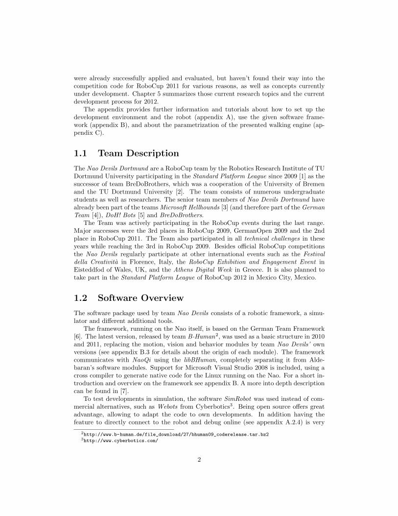
were already successfully applied and evaluated, but haven’t found their way into thecompetition code for RoboCup 2011 for various reasons, as well as concepts currentlyunder development. Chapter 5 summarizes those current research topics and the currentdevelopment process for 2012.
The appendix provides further information and tutorials about how to set up thedevelopment environment and the robot (appendix A), use the given software frame-work (appendix B), and about the parametrization of the presented walking engine (ap-pendix C).
1.1 Team Description
The Nao Devils Dortmund are a RoboCup team by the Robotics Research Institute of TUDortmund University participating in the Standard Platform League since 2009 [1] as thesuccessor of team BreDoBrothers, which was a cooperation of the University of Bremenand the TU Dortmund University [2]. The team consists of numerous undergraduatestudents as well as researchers. The senior team members of Nao Devils Dortmund havealready been part of the teams Microsoft Hellhounds [3] (and therefore part of the GermanTeam [4]), DoH! Bots [5] and BreDoBrothers.
The Team was actively participating in the RoboCup events during the last range.Major successes were the 3rd places in RoboCup 2009, GermanOpen 2009 and the 2ndplace in RoboCup 2011. The Team also participated in all technical challenges in theseyears while reaching the 3rd in RoboCup 2009. Besides official RoboCup competitionsthe Nao Devils regularly participate at other international events such as the Festivaldella Creativita in Florence, Italy, the RoboCup Exhibition and Engagement Event inEisteddfod of Wales, UK, and the Athens Digital Week in Greece. It is also planned totake part in the Standard Platform League of RoboCup 2012 in Mexico City, Mexico.
1.2 Software Overview
The software package used by team Nao Devils consists of a robotic framework, a simu-lator and different additional tools.
The framework, running on the Nao itself, is based on the German Team Framework[6]. The latest version, released by team B-Human2, was used as a basic structure in 2010and 2011, replacing the motion, vision and behavior modules by team Nao Devils’ ownversions (see appendix B.3 for details about the origin of each module). The frameworkcommunicates with NaoQi using the libBHuman, completely separating it from Alde-baran’s software modules. Support for Microsoft Visual Studio 2008 is included, using across compiler to generate native code for the Linux running on the Nao. For a short in-troduction and overview on the framework see appendix B. A more into depth descriptioncan be found in [7].
To test developments in simulation, the software SimRobot was used instead of com-mercial alternatives, such as Webots from Cyberbotics3. Being open source offers greatadvantage, allowing to adapt the code to own developments. In addition having thefeature to directly connect to the robot and debug online (see appendix A.2.4) is very
2http://www.b-human.de/file_download/27/bhuman09_coderelease.tar.bz23http://www.cyberbotics.com/
2
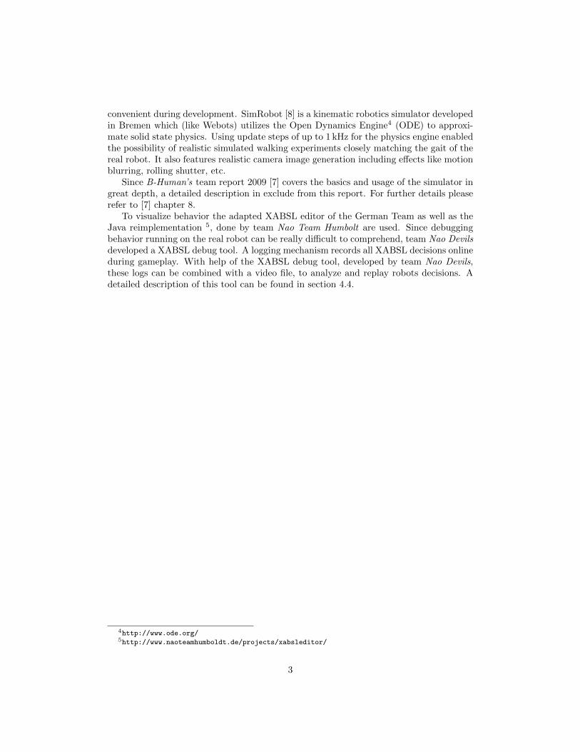
convenient during development. SimRobot [8] is a kinematic robotics simulator developedin Bremen which (like Webots) utilizes the Open Dynamics Engine4 (ODE) to approxi-mate solid state physics. Using update steps of up to 1 kHz for the physics engine enabledthe possibility of realistic simulated walking experiments closely matching the gait of thereal robot. It also features realistic camera image generation including effects like motionblurring, rolling shutter, etc.
Since B-Human’s team report 2009 [7] covers the basics and usage of the simulator ingreat depth, a detailed description in exclude from this report. For further details pleaserefer to [7] chapter 8.
To visualize behavior the adapted XABSL editor of the German Team as well as theJava reimplementation 5, done by team Nao Team Humbolt are used. Since debuggingbehavior running on the real robot can be really difficult to comprehend, team Nao Devilsdeveloped a XABSL debug tool. A logging mechanism records all XABSL decisions onlineduring gameplay. With help of the XABSL debug tool, developed by team Nao Devils,these logs can be combined with a video file, to analyze and replay robots decisions. Adetailed description of this tool can be found in section 4.4.
4http://www.ode.org/5http://www.naoteamhumboldt.de/projects/xabsleditor/
3
Chapter 2
Motion
The main challenge of humanoid robotics certainly are the various aspects of motiongeneration and biped walking. Dortmund has participated in the Humanoid Kid-SizeLeague during Robocup 2007 as DoH! Bots [5] and before in RoboCup 2006 as the jointteam BreDoBrothers together with Bremen University. Hence there has already beensome experience in the research area of two-legged walking even before participating inthe Nao Standard Platform League of 2008 as the rejoined BreDoBrothers.
The kinematic structure of the Nao has some special characteristics that make itstand out from other humanoid robot platforms. Aldebaran Robotics implemented theHipYawPitch joints using only one servo motor. This fact links both joints and therebymakes it impossible to move one of the two without moving the other. Hence the kinematicchains of both legs are coupled. In addition both joints are tilted by 45 degrees. Thesestructural differences to the humanoid robots used in previous years in the HumanoidLeague result in an unusual workspace of the feet. Therefore existing movement conceptshad to be adjusted or redeveloped from scratch. The leg motion is realized by an inversekinematic calculated with the help of analytical methods for the stance leg. The swingingleg end position is then calculated with the constraint of the HipYawPitch joint neededfor the support foot. This closed form solution to the inverse kinematic problem for theNao has been developed in Dortmund and used since RoboCup 2008 when other teamsas well as Aldebaran themselves still used iterative approximations.
2.1 Walking
In the past different walking engines have been developed following the concept of statictrajectories. The parameters of these precalculated trajectories are optimized with algo-rithms of the research field of Computational Intelligence. This allows a special adaptionto the used robot hardware and environmental conditions. Approaches to move two leggedrobots with the help of predefined foot trajectories are common in the Humanoid Kid-SizeLeague and offer good results. Nonetheless with such algorithms directly incorporatingsensor feedback is much less intuitive. Sensing and reacting to external disturbances how-ever is essential in robot soccer. During a game these disturbances come inevitably in theform of different ground-friction areas or bulges of the carpet. Additionally contacts withother players or the ball are partly unpreventable and result in external forces acting on
4
the body of the robot.To avoid regular recalibration and repeated parameter optimization the walking al-
gorithm should also be robust against systematic deviations from its internal model.Trajectory based walking approaches often need to be tweaked to perform optimally oneach real robot. But some parameters of this robot are subject to change during the life-time of a robot or even during a game of soccer. The reasons could manifold for instanceas joint decalibration, wear out of the mechanical structure or thermic drift of the servodue to heating. Recalibrating for each such occurrence costs much time at best and issimply not possible in many situations.
The robot Nao comes equipped with the wide range of sensors capable of measuringforces acting on the body, namely an accelerometer, gyroscope and force sensors in thefeet. To overcome the drawback of a static trajectory playback, team Nao Devils devel-oped a walking engine capable of generating online dynamically stable walking patternswith the use of sensor feedback.
2.1.1 Dortmund Walking Engine
A common way to determine and ensure the stability of the robot utilizes the zero momentpoint (ZMP) [9]. The ZMP is the point on the ground where the tipping moment actingon the robot, due to gravity and inertia forces, equals zero. Therefore the ZMP has tobe inside the support polygon for a stable walk, since an uncompensated tipping momentresults in instability and fall. This requirement can be addressed in two ways.
On the one hand, it is possible to measure an approximated ZMP with the accelerationsensors of the Nao by using equations 2.1 and 2.2 [10]. Then the position of the approx-imated ZMP on the floor is (px, py). Note that this ZMP can be outside the supportpolygon and therefore follows the concept of the fictitious ZMP.
px = x− zhgx (2.1)
py = y − zhgy (2.2)
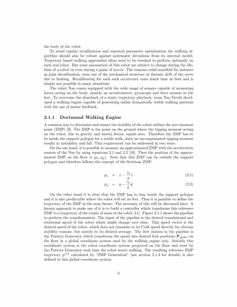
On the other hand it is clear that the ZMP has to stay inside the support polygonand it is also predictable where the robot will set its feet. Thus it is possible to define thetrajectory of the ZMP in the near future. The necessity of this will be discussed later. Aknown approach to make use of it is to build a controller which transforms this referenceZMP to a trajectory of the center of mass of the robot [11]. Figure 2.1.1 shows the pipelineto perform the transformation. The input of the pipeline is the desired translational androtational speed of the robot which might change over time. This speed vector is thedesired speed of the robot, which does not translate to its CoM speed directly for obviousstability reasons, but merely to its desired average. The first station in the pipeline isthe Pattern Generator which transforms the speed into desired foot positions Pglobal onthe floor in a global coordinate system used by the walking engine only. Initially thiscoordinate system is the robot coordinate system projected on the floor and reset bythe Pattern Generator each time the robot starts walking. The resulting reference ZMPtrajectory pref calculated by “ZMP Generation” (see section 2.1.3 for details) is alsodefined in this global coordinate system.
5

PatternGenerator ZMP Generation
ZMP/IPController
InverseKinematic
ArmMovement
Local CoMCalculation
Robot
Target Angles
Measured AnglesMeasured ZMP
-+
+
Swinging LegController
Footsteps
DesiredZMP
TargetCoM
Position
ActualCoM
Position
CompleteFoot Positions
Global CoMCalculation
Measured Angles
Figure 2.1: Control structure visualization of the walking pattern generation process.Data expressed in the robot coordinate system are represented by a blue line and dataexpressed in the global coordinate system is represented by a red line.
6
The core of the system is the ZMP/IP-Controller, which transforms the reference ZMPto a corresponding CoM trajectory (Rref ) in the global coordinate system as mentionedabove. The robot’s CoM relative to its coordinate frame (Rlocal) is given by the frameworkbased on measured angles. Equation 2.3 provides the foot positions in a robot centeredcoordinate frame.
Probot (t) = Pglobal (t)−Rref (t) + Rlocal (t) (2.3)
Those can subsequently be transformed into leg joint angles using inverse kinematics.Finally the leg angles are complemented with arm angles which are calculated using thex coordinates of the feet.
2.1.2 The ZMP/IP-Controller
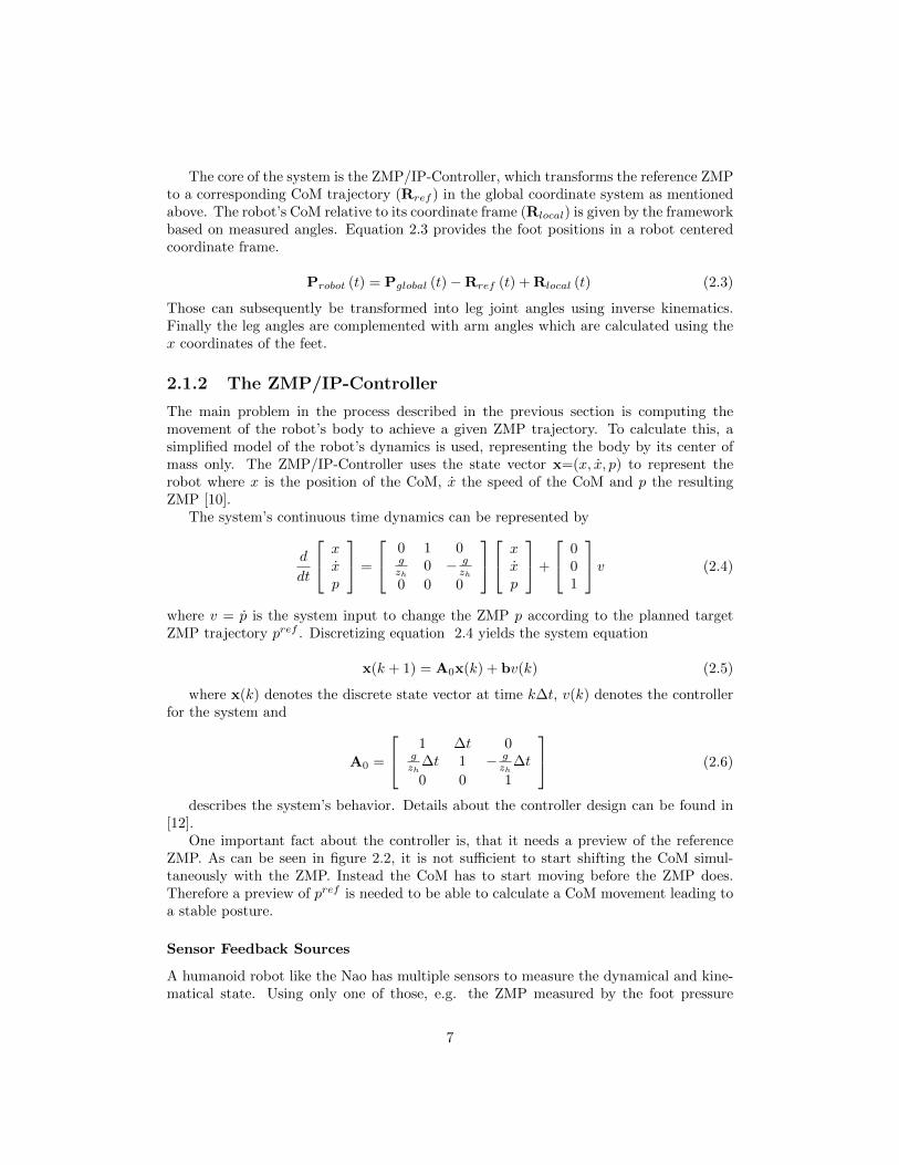
The main problem in the process described in the previous section is computing themovement of the robot’s body to achieve a given ZMP trajectory. To calculate this, asimplified model of the robot’s dynamics is used, representing the body by its center ofmass only. The ZMP/IP-Controller uses the state vector x=(x, x, p) to represent therobot where x is the position of the CoM, x the speed of the CoM and p the resultingZMP [10].
The system’s continuous time dynamics can be represented by
d
dt
xxp
=
0 1 0gzh
0 − gzh
0 0 0
xxp
+
001
v (2.4)
where v = p is the system input to change the ZMP p according to the planned targetZMP trajectory pref . Discretizing equation 2.4 yields the system equation
x(k + 1) = A0x(k) + bv(k) (2.5)
where x(k) denotes the discrete state vector at time k∆t, v(k) denotes the controllerfor the system and
A0 =
1 ∆t 0gzh
∆t 1 − gzh
∆t
0 0 1
(2.6)
describes the system’s behavior. Details about the controller design can be found in[12].
One important fact about the controller is, that it needs a preview of the referenceZMP. As can be seen in figure 2.2, it is not sufficient to start shifting the CoM simul-taneously with the ZMP. Instead the CoM has to start moving before the ZMP does.Therefore a preview of pref is needed to be able to calculate a CoM movement leading toa stable posture.
Sensor Feedback Sources
A humanoid robot like the Nao has multiple sensors to measure the dynamical and kine-matical state. Using only one of those, e.g. the ZMP measured by the foot pressure
7

Figure 2.2: CoM motion required to achieve a given ZMP trajectory.
Figure 2.3: Control system with sensor feedback using an observer.
sensors or the acceleration, has some disadvantages, like noisy data or measurement de-lays. A common way to cope with these problems is to implement a sensor fusion usinga kalman filter. Looking at the control structure of the ZMP/IP-Controller reveals thatparts of the state vector can be measured, namely the position of the center of massxsensor(k) and the actual ZMP psensor(k). The first can be calculated using the center ofmass positions ci of each link expressed in the coordinate frame of link i:
xsensor(k) = Tws (k) ·
(1∑l ml
·∑i
T sOi
(k) · ci ·mi
)(2.7)
where
• s is the coordinate system of the support foot.
• w is the world coordinate system.
• Oi is the coordinate system of link i.
• mi is the mass of link i.
• T ji (k) is the homogeneous coordinate system transformation matrix from coordinate
system i to j.
The later is the weighted average of the data measured by each pressure sensor in thefeet. In case of the Nao robot the CoP for the left psensorleft (k) and right foot psensorright (k) aregiven by the API and must be combined:
8

psensor(k) =fl (k)
F· Tw
Ol(k) · psensorleft (k) +
fr (k)
F· Tw
Or(k) · psensorright (k) (2.8)
where
• Ol, Or is the coordinate system of left and right foot respectively.
• fl (k), fr (k) is the force exerted on the left and right foot respectively.
• F = fl (k) + fr (k) is the overall force exerted on the robot.
This kind of ZMP measurement has the same limitation as the definition of the ZMP,it is bounded to the supporting area. As a result, the ZMP will be measured at the edgeof the support area when the robot tilts. The measurement of the center of mass positionis limited in a similar way. The result of flexibilities and tolerances in the joints can bemeasured, but not the result of the tilt of the robot. This is not necessarily a disad-vantage, since it limits the reaction of the robot to disturbances to securely executablemovements, especially if the robots falls down. The limitation of the CoM measurementalso corresponds to the ZMP measurement limits.
Regarding the coordinate system transformations, there is one noticeable point. Thetransformations to the world coordinate system Tw
Oi(k) and other transformations are
seperated. The reason for that is the way of calculating. The transformations betweenthe coordinate systems of the links are calculated using forward kinematics and measuredangles. However, the position and orientation of the feet in the world coordinate systemcannot be measured directly. Possible sources would the self localization or the odometrycalculated by integrating the acceleration sensor, both combined with forward kinematics.But these sources are inaccurate and lead to large noise in the measured CoM and ZMPpositions. Measurable errors during a walk are much lower than these measurement errorsand it would be not possible to react correctly. Therefore the target foot positions andorientations given by the Pattern Generator are used for Tw
Oi(k).
Integration of the Measurements, a Sensor Fusion
In the last chapter two measurable values of the state vector x(k) are presented. Themeasurable output of the system given by equation 2.5 can now be defined as
y (k) = c · x(k)=
[xsensor(k)psensor(k)
](2.9)
with
c =
[1 0 00 0 1
](2.10)
Since not the full state can be measured, an observer is needed. Figure 2.3 showsthe overall system configuration. The observer is put in parallel to the real robot andreceives the same output of the controller to estimate the behavior of the real system andis supported by the measurements of the ZMP and the CoM. Derived from equations 2.5and 2.9 the observer can be defined as follows:
x(k + 1) = A0x(k) + L [y(k)− cx(k)] + bu(k). (2.11)
9
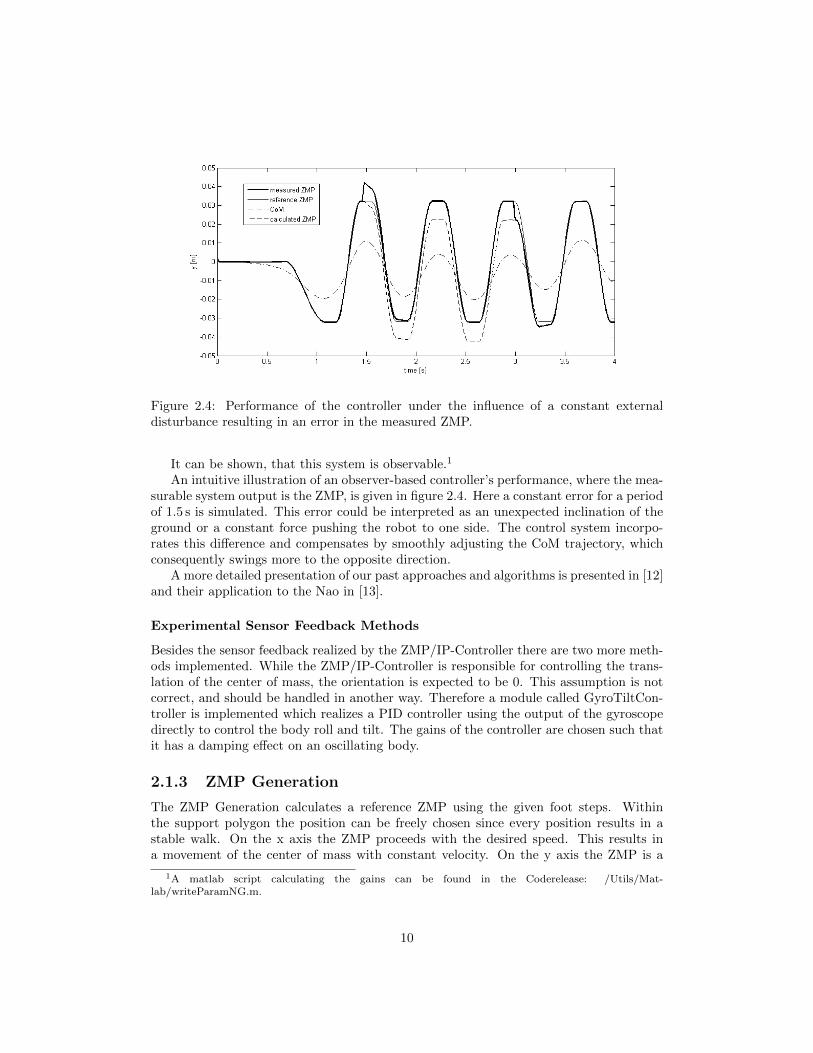
Figure 2.4: Performance of the controller under the influence of a constant externaldisturbance resulting in an error in the measured ZMP.
It can be shown, that this system is observable.1
An intuitive illustration of an observer-based controller’s performance, where the mea-surable system output is the ZMP, is given in figure 2.4. Here a constant error for a periodof 1.5 s is simulated. This error could be interpreted as an unexpected inclination of theground or a constant force pushing the robot to one side. The control system incorpo-rates this difference and compensates by smoothly adjusting the CoM trajectory, whichconsequently swings more to the opposite direction.
A more detailed presentation of our past approaches and algorithms is presented in [12]and their application to the Nao in [13].
Experimental Sensor Feedback Methods
Besides the sensor feedback realized by the ZMP/IP-Controller there are two more meth-ods implemented. While the ZMP/IP-Controller is responsible for controlling the trans-lation of the center of mass, the orientation is expected to be 0. This assumption is notcorrect, and should be handled in another way. Therefore a module called GyroTiltCon-troller is implemented which realizes a PID controller using the output of the gyroscopedirectly to control the body roll and tilt. The gains of the controller are chosen such thatit has a damping effect on an oscillating body.
2.1.3 ZMP Generation
The ZMP Generation calculates a reference ZMP using the given foot steps. Withinthe support polygon the position can be freely chosen since every position results in astable walk. On the x axis the ZMP proceeds with the desired speed. This results ina movement of the center of mass with constant velocity. On the y axis the ZMP is a
1A matlab script calculating the gains can be found in the Coderelease: /Utils/Mat-lab/writeParamNG.m.
10

x
y
x
y
Figure 2.5: The control polygon consists of 4 points per foot with constants coordinateswithin the respective coordinate frame. In this example a positive x speed is assumed fora better visualization.
2 2.5 3 3.5 4 4.5 5 5.5 6−0.06
−0.04
−0.02
0
0.02
0.04
0.06
Time [s]
y [m
]
Figure 2.6: Resulting reference ZMP along the y axis.
11
Bezier curve with a control polygon of 4 points and dimension 1. The coordinate of eachpoint is constant within the coordinate system of the respective foot. Figure 2.5 gives anexample. In the right single support phase the control polygon is Pr = {p1, p2, p3, p4}.The same applies to the other single support phase. In the double support phase thecontrol polygon consists of the points p4, p
′1, p′2, p5, where p′1 and p′2 are the same point in
the middle of p4 and p5. This leads to a smooth transition between the single and doublesupport phases. Figure 2.6 shows the resulting reference ZMP along the y axis.
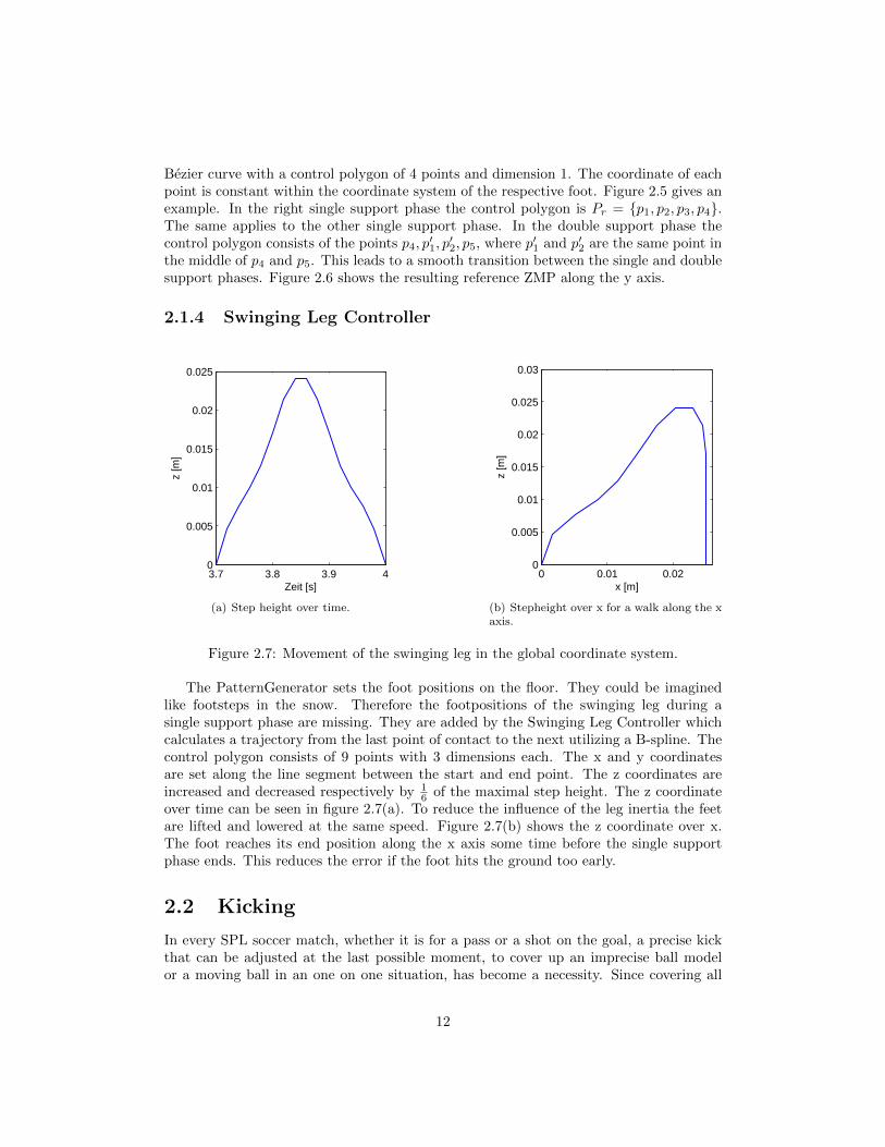
2.1.4 Swinging Leg Controller
3.7 3.8 3.9 40
0.005
0.01
0.015
0.02
0.025
Zeit [s]
z [m
]
(a) Step height over time.
0 0.01 0.020
0.005
0.01
0.015
0.02
0.025
0.03
x [m]
z [m
]
(b) Stepheight over x for a walk along the xaxis.
Figure 2.7: Movement of the swinging leg in the global coordinate system.
The PatternGenerator sets the foot positions on the floor. They could be imaginedlike footsteps in the snow. Therefore the footpositions of the swinging leg during asingle support phase are missing. They are added by the Swinging Leg Controller whichcalculates a trajectory from the last point of contact to the next utilizing a B-spline. Thecontrol polygon consists of 9 points with 3 dimensions each. The x and y coordinatesare set along the line segment between the start and end point. The z coordinates areincreased and decreased respectively by 1
6 of the maximal step height. The z coordinateover time can be seen in figure 2.7(a). To reduce the influence of the leg inertia the feetare lifted and lowered at the same speed. Figure 2.7(b) shows the z coordinate over x.The foot reaches its end position along the x axis some time before the single supportphase ends. This reduces the error if the foot hits the ground too early.
2.2 Kicking
In every SPL soccer match, whether it is for a pass or a shot on the goal, a precise kickthat can be adjusted at the last possible moment, to cover up an imprecise ball modelor a moving ball in an one on one situation, has become a necessity. Since covering all
12

possible kick angles and strengths with Special Actions (see section 2.3) is simply notpossible, a dynamic kick was needed.
Our current implementation uses the inverse kinematic from our walking engine tomove the kicking foot towards the ball. With a fast kick execution time, the stabilityof the robot can hardly be ensured with any kind of reactive controller. Therefore weconcentrated on a implementation that works without a controller and still is able toexecute a stable kick with all desired angles and strengths. The kick motion needs onlyone input, the kick target: a field position relative to the robot.
The main focus in the development for our kick was its stability while still being ableto kick hard. Therefore the kick process is divided into several phases (see figure 2.8):
• lean - shift the robots weight to the standing foot
• prepare - move the foot to a point near the ball
• execute - a fast straight motion towards the ball
• prepare back - back to the position after lean
• lean back - back to the original robots position (standing)
The seperation into these phases allow a parameterization of the kick which can beadjusted and optimized easily. After the leaning process, our kick takes the relative ballcoordinates from our ball model at the beginning of the prepare phase, moves the footto a point in front of the ball so that the execute phase can kick the ball in one straightmove of the foot in the desired direction. For this, the kicking foot origin is placed in afixed distance to the ball on the the circle that this specific distance creates. Due to thedifferent trajectories resulting from a sidekick compared to a frontkick, seperate leaningangles for those motions are used and, since the foot of the Nao robot is not completelysmooth or round, the kicking angle is not entirely free. Currently, the kicking angle islimited from 0 to 25 degrees for a frontkick and from 65 to 90 degrees for a sidekick, whichis quite enough for almost any real game situation.
After the kicking foot has been brought into position, the kicking motion itself is donebefore the robot begins a reverse leaning process to again ensure its stability.
2.3 Special Actions
All movements except walking and kicking are executed by playback of predefined motionscalled Special Actions. These movements consist of certain robot postures called keyframes and transition times between these. Using these transition times the movementbetween the key frames is executed as a synchronous point-to-point movement in the jointspace. Such movements can be designed easily by concatenating recorded key frames.
13
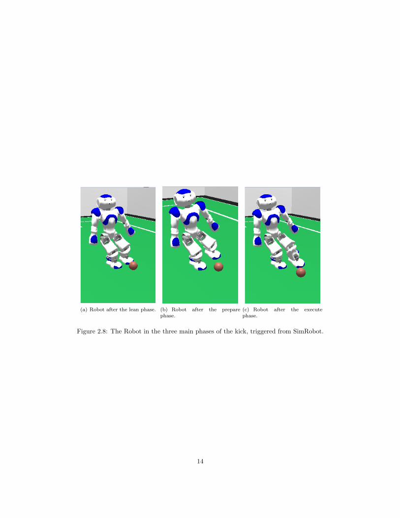
(a) Robot after the lean phase. (b) Robot after the preparephase.
(c) Robot after the executephase.
Figure 2.8: The Robot in the three main phases of the kick, triggered from SimRobot.
14

Chapter 3
Cognition
From the variety of Nao’s sensors only microphones, the camera and sonar sensors canpotentially be used to gain knowledge about the robot’s surroundings. The microphoneshaven’t been used so far and are not expected to give any advantage. The sonar sensorsprovide distance information of the free space in front of the robot and can be used forobstacle detection. However, the usage of these sensors depends on maintaining a strictlyvertical torso or at least tracking its tilt precisely since otherwise the ground might givefalse positives due to the wide conic spreading of the sound waves. Additionally, forcertain fast walk types the swinging arms were observed to generate such false positives,too, and the sonar sensor hardware in general is currently unreliable and often does notrecover from failure once the robot has fallen down. Thus for exteroceptive perceptionthe robot greatly relies on its camera mounted in the head.
The following chapter describes the information flow in the cognition process startingfrom image processing and its sub-tasks in section 3.1. Special focus is given to new devel-opments since 2009, meaning an improved line and center circle detection (see section 3.2)and a new localization module based on a multiple-hypotheses unscented Kalman filter(see section 3.3). Finally section 3.5 gives an outlook about current research that did notfind its way into the code for RoboCup 2010, yet, but is expected to be applied in 2011.
3.1 Image Processing
The vision system used for the Nao in the RoboCups 2008 to 2011 is based on the MicrosoftHellhounds’ development of 2007 [14]. The key idea is to use as much a-priori informationas possible to reduce both the scanning effort and the subsequent calculations needed.To process only a small fraction of all pixels the image is scanned along scan lines ofvarying length depending on the horizon’s projection in the image (see fig. 3.1). Thesescan lines are projections of radial lines originating from the point on the field belowthe camera center. Keeping the angular difference constant allows the implicit usage ofthis information during the scanning process, optimizes transformations between imageand field coordinate systems and significantly simplifies the inter-scan-line clustering andreasoning about detected objects. In case of ambiguity additional verification scans arecarried out. A sparse second set of horizontal scan lines is introduced to detect far goals.
All relevant objects and features are extracted with high accuracy and detection rates.
15

Figure 3.1: Image scanned along projections of radial lines on the field.
(a) Camera Image. (b) Field view.
Figure 3.2: Objects and features recognized in the camera image.
16
(a) Camera Image. (b) Field view.
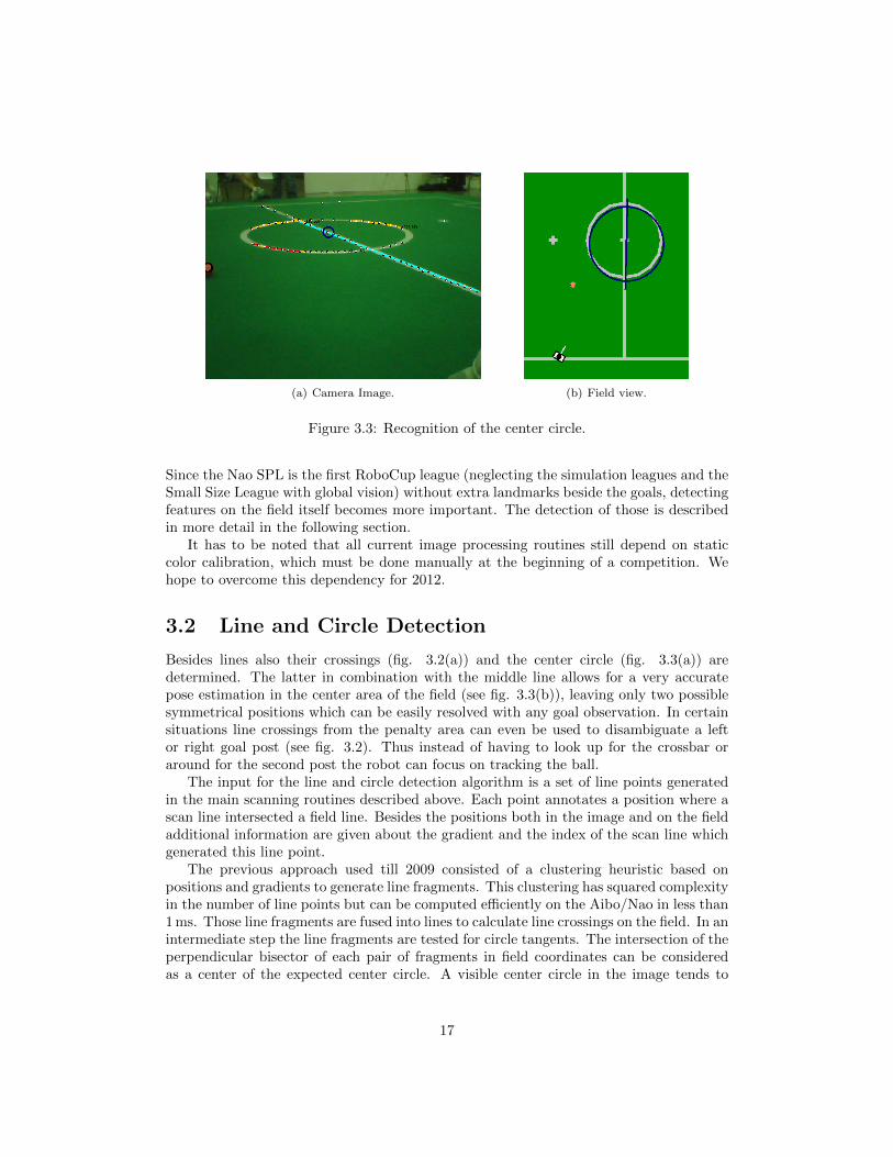
Figure 3.3: Recognition of the center circle.
Since the Nao SPL is the first RoboCup league (neglecting the simulation leagues and theSmall Size League with global vision) without extra landmarks beside the goals, detectingfeatures on the field itself becomes more important. The detection of those is describedin more detail in the following section.
It has to be noted that all current image processing routines still depend on staticcolor calibration, which must be done manually at the beginning of a competition. Wehope to overcome this dependency for 2012.
3.2 Line and Circle Detection
Besides lines also their crossings (fig. 3.2(a)) and the center circle (fig. 3.3(a)) aredetermined. The latter in combination with the middle line allows for a very accuratepose estimation in the center area of the field (see fig. 3.3(b)), leaving only two possiblesymmetrical positions which can be easily resolved with any goal observation. In certainsituations line crossings from the penalty area can even be used to disambiguate a leftor right goal post (see fig. 3.2). Thus instead of having to look up for the crossbar oraround for the second post the robot can focus on tracking the ball.
The input for the line and circle detection algorithm is a set of line points generatedin the main scanning routines described above. Each point annotates a position where ascan line intersected a field line. Besides the positions both in the image and on the fieldadditional information are given about the gradient and the index of the scan line whichgenerated this line point.
The previous approach used till 2009 consisted of a clustering heuristic based onpositions and gradients to generate line fragments. This clustering has squared complexityin the number of line points but can be computed efficiently on the Aibo/Nao in less than1 ms. Those line fragments are fused into lines to calculate line crossings on the field. In anintermediate step the line fragments are tested for circle tangents. The intersection of theperpendicular bisector of each pair of fragments in field coordinates can be consideredas a center of the expected center circle. A visible center circle in the image tends to
17
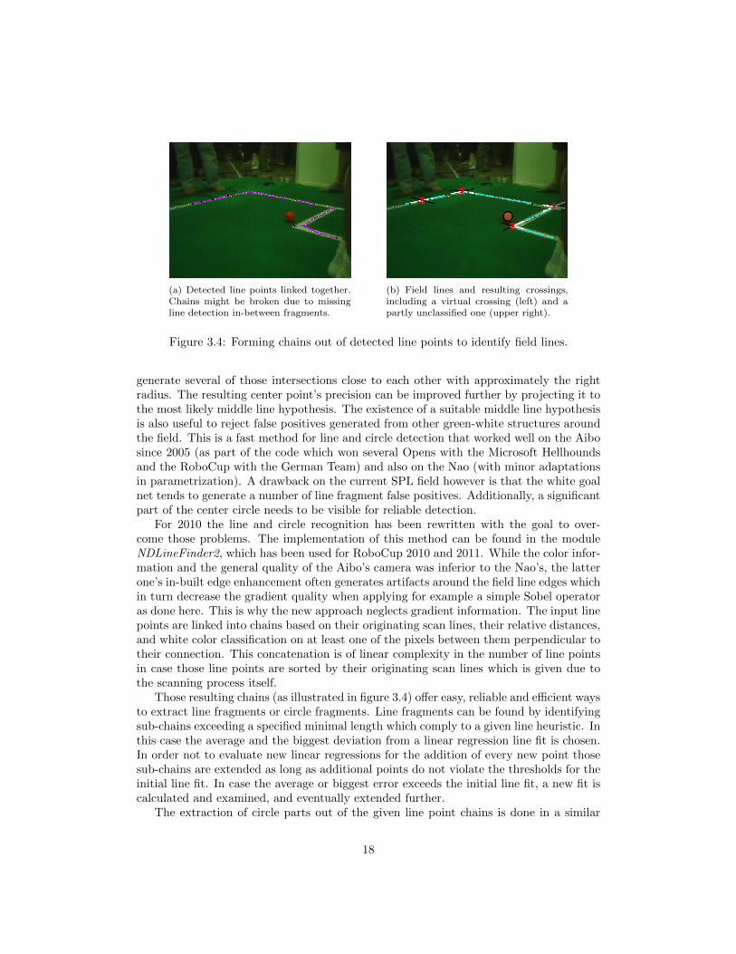
(a) Detected line points linked together.Chains might be broken due to missingline detection in-between fragments.
(b) Field lines and resulting crossings,including a virtual crossing (left) and apartly unclassified one (upper right).
Figure 3.4: Forming chains out of detected line points to identify field lines.
generate several of those intersections close to each other with approximately the rightradius. The resulting center point’s precision can be improved further by projecting it tothe most likely middle line hypothesis. The existence of a suitable middle line hypothesisis also useful to reject false positives generated from other green-white structures aroundthe field. This is a fast method for line and circle detection that worked well on the Aibosince 2005 (as part of the code which won several Opens with the Microsoft Hellhoundsand the RoboCup with the German Team) and also on the Nao (with minor adaptationsin parametrization). A drawback on the current SPL field however is that the white goalnet tends to generate a number of line fragment false positives. Additionally, a significantpart of the center circle needs to be visible for reliable detection.
For 2010 the line and circle recognition has been rewritten with the goal to over-come those problems. The implementation of this method can be found in the moduleNDLineFinder2, which has been used for RoboCup 2010 and 2011. While the color infor-mation and the general quality of the Aibo’s camera was inferior to the Nao’s, the latterone’s in-built edge enhancement often generates artifacts around the field line edges whichin turn decrease the gradient quality when applying for example a simple Sobel operatoras done here. This is why the new approach neglects gradient information. The input linepoints are linked into chains based on their originating scan lines, their relative distances,and white color classification on at least one of the pixels between them perpendicular totheir connection. This concatenation is of linear complexity in the number of line pointsin case those line points are sorted by their originating scan lines which is given due tothe scanning process itself.
Those resulting chains (as illustrated in figure 3.4) offer easy, reliable and efficient waysto extract line fragments or circle fragments. Line fragments can be found by identifyingsub-chains exceeding a specified minimal length which comply to a given line heuristic. Inthis case the average and the biggest deviation from a linear regression line fit is chosen.In order not to evaluate new linear regressions for the addition of every new point thosesub-chains are extended as long as additional points do not violate the thresholds for theinitial line fit. In case the average or biggest error exceeds the initial line fit, a new fit iscalculated and examined, and eventually extended further.
The extraction of circle parts out of the given line point chains is done in a similar
18
(a) Detected line points linked together. (b) Classification of field line and circlefragment.
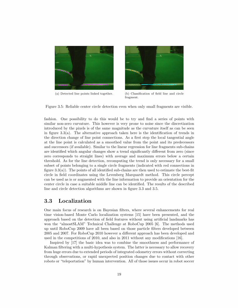
Figure 3.5: Reliable center circle detection even when only small fragments are visible.
fashion. One possibility to do this would be to try and find a series of points withsimilar non-zero curvature. This however is very prone to noise since the discretizationintroduced by the pixels is of the same magnitude as the curvature itself as can be seenin figure 3.3(a). The alternative approach taken here is the identification of trends inthe direction change of line point connections. As a first step the local tangential angleat the line point is calculated as a smoothed value from the point and its predecessorsand successors (if available). Similar to the linear regression for line fragments sub-chainsare identified which angular changes show a trend significantly different from zero (sincezero corresponds to straight lines) with average and maximum errors below a certainthreshold. As for the line detection, recomputing the trend is only necessary for a smallsubset of points belonging to a single circle fragments (indicated with red connections infigure 3.3(a)). The points of all identified sub-chains are then used to estimate the best-fitcircle in field coordinates using the Levenberg Marquardt method. This circle perceptcan be used as is or augmented with the line information to provide an orientation for thecenter circle in case a suitable middle line can be identified. The results of the describedline and circle detection algorithms are shown in figure 3.3 and 3.5.
3.3 Localization
One main focus of research is on Bayesian filters, where several enhancements for realtime vision-based Monte Carlo localization systems [15] have been presented, and theapproach based on the detection of field features without using artificial landmarks haswon the “almostSLAM” Technical Challenge at RoboCup 2005 [6]. The methods usedup until RoboCup 2009 have all been based on those particle filters developed between2005 and 2007. For RoboCup 2010 however a different approach has been developed andused in the competitions of 2010, and also in 2011 without any modifications [16].
Inspired by [17] the basic idea was to combine the smoothness and performance ofKalman filtering with a multi-hypothesis system. The latter is necessary to allow recoveryfrom huge errors due to extended periods of integrated odometry errors without correctingthrough observations, or rapid unexpected position changes due to contact with otherrobots or “teleportation” by human intervention. All of those issues occur in robot soccer
19
games and are amplified by the huge odometry errors inherent in fast biped walking.A classic Kalman filter applied to localization in a SPL scenario can only be used for
position tracking, and only as long as the estimate does not deviate too much from thetrue positions. Most perceptions on a SPL field are ambiguous, so the sensor update willonly be done with the most likely data association. At the same time, the perceptionof field features like field line crossings is often uncertain so that L- and T-crossings cannot be distinguished (e.g. as in figure 3.4(b)). In such cases wrong associations tend todrive the estimation further away from the true position. Recovery from such situations isonly possible when assigning huge weights (e.g. small observation covariances) to uniqueperceptions like observing both goal posts in the same frame which then decreases therobustness against false perceptions originating from the audience around the field.
This problem is addressed in [17] with a sum-of-Gaussians Kalman filter, where eachGaussian is split into several new ones representing the results of different associationchoices. Applying all possible data associations to every hypothesis generates exponentialgrowth which needs cutting back shortly after by applying pruning heuristics and fusingsimilar Gaussians to prevent an explosion of computational complexity. Thus lots ofprocessing time is wasted on creating and destroying new hypothesis which are eitherunlikely or very similar to the ones that already exist.
A different approach is implemented in the module MultiUKFSelfLocator. Only fewnew hypotheses are generated periodically at positions with high probability based only onrecent sensor information. Those hypotheses are only updated using data that lies insidea certain expectation threshold. Non-linearity in the sensor model is addressed using theunscented transformation technique. Several other approximations and simplificationsresult in a localization method that is an order of magnitude faster than the previouslyused particle filter while providing superior localization quality and increased robustnessto false positive perceptions (see figure 3.6). A more detailed presentation of the approachand its stochastic soundness is given in [16].
3.4 Distributed World Modeling
Current work includes robust cooperative world modeling and localization using conceptsbased on multi robot SLAM [18], as well as using probabilistic physics simulation andestimation to improve the robot’s state estimation and odometry information [19]. Keep-ing track of the robot’s dynamic environment opens the possibility for tactical behaviordecisions beyond simple reactive behaviors which are currently in use.
The algorithm described in [18] estimates the robot’s location and the surroundingdynamic objects simultaneously. In this joint modeling of the robot’s state a particlefilter estimates the robot’s pose. Clusters of particles are combined into super-particleswhich map the dynamic environment using a number of Kalman filters. This representsan approximation of FastSLAM and both decreases the integration of odometry errorcompared to robot-centric local modeling (see figure 3.7) and allows resolving multi-modal localization belief states using shared information. The approach even preservesits SLAM functionality and is able to maintain a robot’s localization based on mappeddynamic obstacles only. A detailed presentation of the approach is presented in [18].
By specifically addressing the heterogeneity of the perceived information and the needto synchronize the estimation between the team of robots the task’s complexity can be
20

-3000 -2000 -1000 0 1000 2000 3000
-2000
-1000
0
1000
2000
GroundTruth
MultiUKF
ParticleFilter
(a) Estimated positions and ground truth on the field.
30 40 50 60 70 80 90 100 110 1200
200
400
600
800
Pos
ition
Err
or [m
m]
30 40 50 60 70 80 90 100 110 1200
10
20
30
40
50
Time [s]
Ab. O
rient
atio
n E
rror [
°]
MultiUKFPartikelf ilterParticleFilterMultiUKF
(b) Errors in pose estimation.
30 40 50 60 70 80 90 100 110 1200
5
10
15
20
25
30
35
40
ParticleFilterMultiUKF
Time [s]
Fram
e-U
pdat
e [m
s]
(c) Localization runtime.
Figure 3.6: Localization of Multiple-Hypotheses UKF compared to previous particle filtersolution (which was used in RoboCup 2009). Both are running in parallel on the Naousing the same perception as input. Ground truth is provided by a camera mountedabove the field.
21

(a) No gain for frequently observed robots. (b) Tracking of infrequently observed robots sig-nificantly improved.
Figure 3.7: Advantage by unified (blue) compared to separate robot-centric modeling(red).
reduced to be in the range of applicability on limited embedded platforms. This module’saverage runtime on the Nao in the configuration used on the RoboCup 2010 would havebeen slightly above 20 ms which would not have allowed to keep a frame rate of 15 Hz oreven 30 Hz. Especially the switch to a motion frame rate of 100 Hz made its applicationimpossible. Additionally the system is based on the outdated particle filter localizationof previous years.
For 2011 parts of this distributed world modeling approach have been integrated withthe new localization system described in section 3.3. Since the UKF localization conceptdoes not allow the transformation of a combined estimator according to the Rao-Blackwelltheorem, the SLAM aspect can not be transferred in this case directly. In the 2011 codeused in the competitions, the SLAM aspects were not fully implemented. The ball androbot modeling is still done in a cooperative way using the approximations describedin [18], but there has been no feedback into the localization and only a single maximum-likelihood hypothesis is maintained at each time.
In the code release accompanying this report there is the possibility to choose betweenlocal models, which are the result of the local aggregation of percepts (percept-buffering,but without periodically flushing the results into the global model, and the global modelitself, which is a fusion of all distributed information. Due to the lack of feedback into arobot’s own localization there are situations where the local model is still to be preferred.Precisely approaching close balls for example requires accurate robot relative informationinstead of the precise global position of the ball on the field. In the global model, theball is more precise in global coordinates, but moderate errors in a robot’s localizationwould have a major impact on the relative positioning, as long as the robot’s pose is notcorrected by the distributed information, too.
3.5 Current Research
The modules and algorithms described in the previous sections 3.1 to 3.3 can all be foundin the code released together with this document. This section summarizes both currentand previous research and experiments for which the transition into the actual soccer
22
code has not been done yet but is expected to influence the code for RoboCup 2012.
3.5.1 Cooperative EKF-SLAM World Modeling
As an Open Challenge presentation at RoboCup 2011 a prototype system for an EKF-SLAM version of the system described in section 3.4 has been presented. It differs fromthe FastSLAM version described above in several aspects which will be discussed, but thetwo most important points are that it is based on the currently used MultiUKFSelfLocator(see section 3.3) and that both the localization and the EKF-SLAM extension togetherare still fast enough to run on the Nao in real-time.
As in [18], the central idea of the approach is to model the localization and all thedynamic elements of the robot’s environment in one full SLAM state, but since the local-ization is not estimated using a particle filter, the full state can not be factorized as inFastSLAM. So to build upon the UKF localization described above, the full state needsto be expressed by a mean and covariance matrix in case of EKF-SLAM world model-ing. The increase of estimation complexity by the high-dimensional state is counteredby aggregation of some of the image processing results into temporary percept-buffers.This has two advantages: On the one hand, highly uncertain single observations can beintegrated into different models with decreased uncertainty before forwarding them tothe EKF-SLAM core algorithm. This can be used at the same time to filter out falsepositives which are not confirmed by more than one single observation. Only those tem-porary models with enough confirmation are forwarded to the distributed modeling anddeleted from the local percept-buffer. Deleting them from the percept-buffer guaranteesthe stochastic independence of different observations originating from the same sourceand prevents the continuous integration of odometry errors over longer periods of time.On the other hand, a second advantage is the decrease in complexity by using the modelsfrom the percept buffers instead of all percepts directly. At the same time, those tempo-rary models or buffered percepts can be shared among a group of robots to cooperativelymodel their environment.
This is applied to full extend with the dynamic features, i.e. the ball and otherrobots. A separate localization module, in itself also a buffer integrating informationfrom static, known world features into a localization belief model, is used analogically tothose percept-buffers, but the state is not deleted periodically after forwarding the beliefto the SLAM part of the algorithm. This localization reflects part of the SLAM state,and changes to this part of the SLAM state are fed back into the localization module’sstate. Thus the virtual localization measurements used to update the SLAM state arebasically the innovation introduced by new static feature observations. Therefore thosemeasurements are still conditionally independent from previous measurements given thecurrent belief state, so the Markov assumption is not violated.
Figure 3.8 illustrates a simple scenario in a simulated environment. The robots in ateam share their information for distributed cooperative modeling. Figure 3.8(b) showsthe resulting model with 2D covariance ellipses extracted from the full state. In thefollowing, one robot looks down and does not see any static field features any more, andboth he and the ball are teleported to another location on the field (see figure 3.9). Theuse of distributed percepts and the modeling of the own pose together with the ones ofother robots and the ball position and velocity allows the robot to not only correct itsposition, but also its orientation.
23

(a) Setup of the robots on the field. (b) World model generated from local and dis-tributed information.
Figure 3.8: Scenario with a team of robots looking around and sharing perception infor-mation to cooperatively model their environment.
(a) Scenario after teleportation of ball anddownwards-looking robot.
(b) World model generated from local and dis-tributed information.
Figure 3.9: Following the situation in figure 3.8, one robot looks down and only seesthe ball but no landmarks, and he and the ball are teleported. The shared informationhowever still allows for a correction of both position and orientation of the robot.
24
This simple experiment shows the potential usefulness of such a combined modeling ofa robot’s dynamic environment and its pose in it. RoboCup SPL games contain periodswhere robots are chasing the ball, approaching it for precise positioning to shoot at thegoal, or even dribbling it. During those periods odometry errors are integrated into therobot’s localization if not countered by frequently looking up at static field features tocorrect the robot’s pose estimation. If looking at the ball also allows the correction ofthose odometry errors, especially the orientation, this is expected to be a clear advantage.
Future work will be to evaluate and tune the systems behavior in real soccer scenariosin order to be able to apply it in regular games in RoboCup 2012. Further work can bedone towards extending this into a multi hypothesis system, but for this more reliableruntime measurements have to be done first.
3.5.2 Active Vision
(a) Ambiguity close to the opponent goal whichcan not be resolved by observing a single goal postalone.
(b) The optimal viewing direction estimated fromthe previous particle distribution.
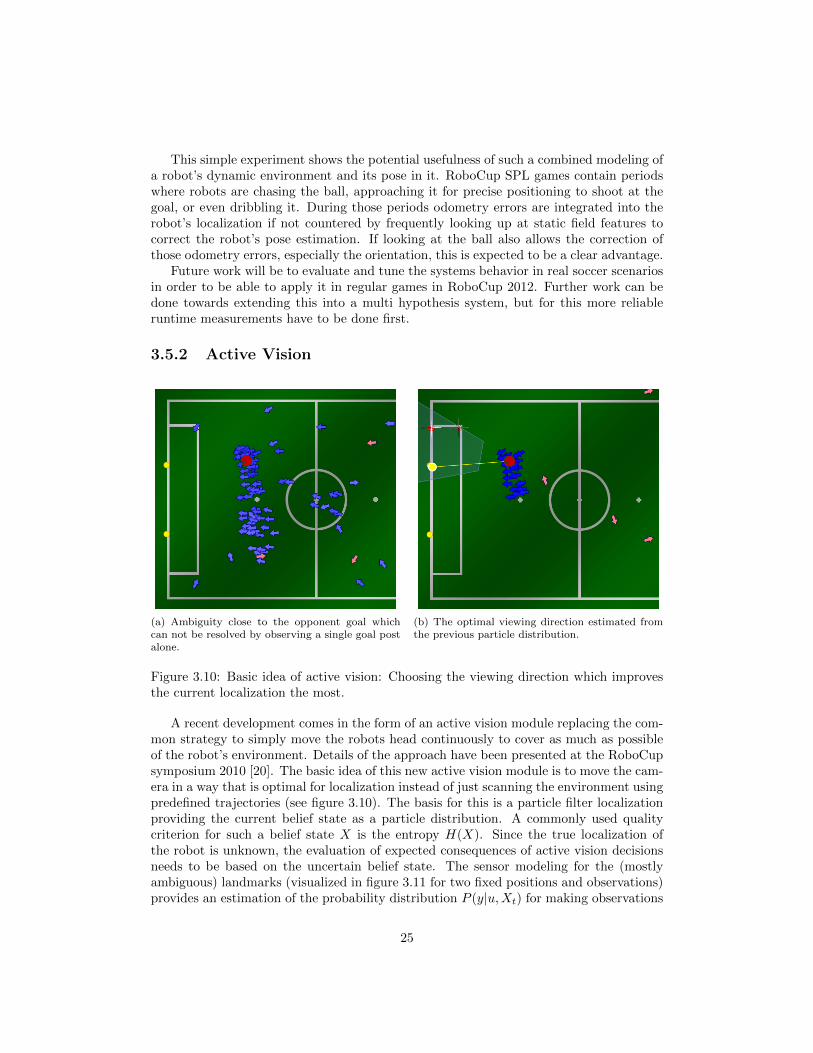
Figure 3.10: Basic idea of active vision: Choosing the viewing direction which improvesthe current localization the most.
A recent development comes in the form of an active vision module replacing the com-mon strategy to simply move the robots head continuously to cover as much as possibleof the robot’s environment. Details of the approach have been presented at the RoboCupsymposium 2010 [20]. The basic idea of this new active vision module is to move the cam-era in a way that is optimal for localization instead of just scanning the environment usingpredefined trajectories (see figure 3.10). The basis for this is a particle filter localizationproviding the current belief state as a particle distribution. A commonly used qualitycriterion for such a belief state X is the entropy H(X). Since the true localization ofthe robot is unknown, the evaluation of expected consequences of active vision decisionsneeds to be based on the uncertain belief state. The sensor modeling for the (mostlyambiguous) landmarks (visualized in figure 3.11 for two fixed positions and observations)provides an estimation of the probability distribution P (y|u,Xt) for making observations
25
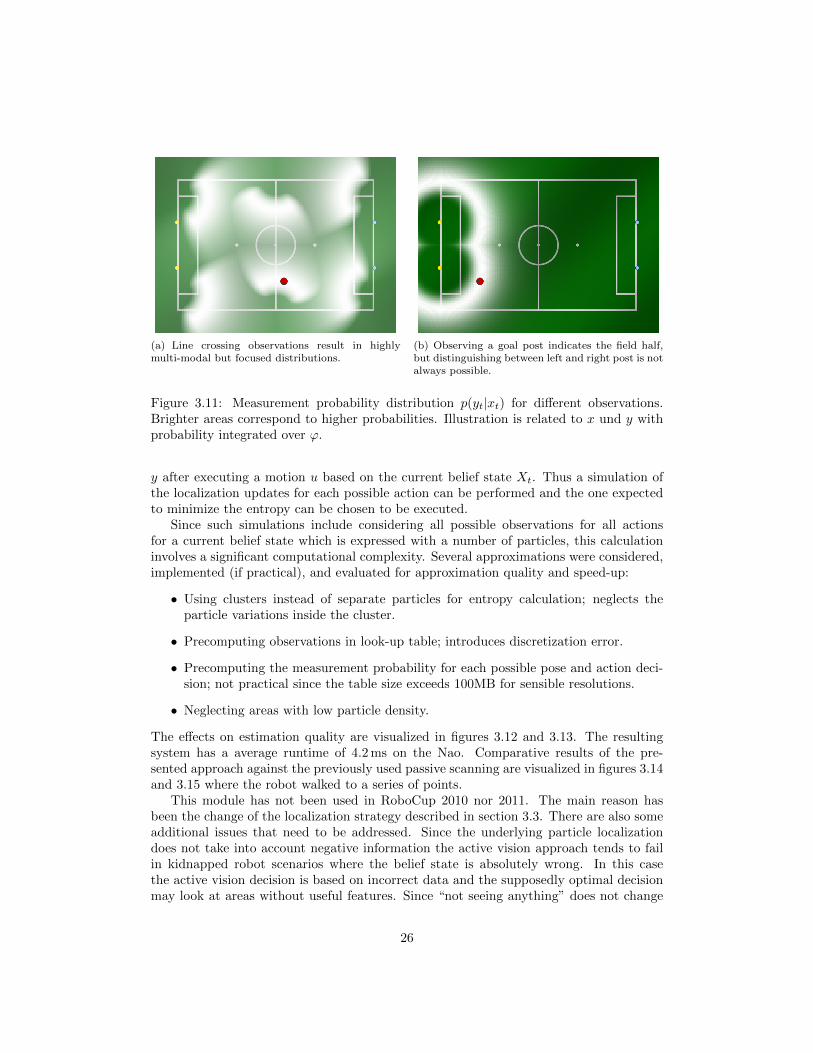
(a) Line crossing observations result in highlymulti-modal but focused distributions.
(b) Observing a goal post indicates the field half,but distinguishing between left and right post is notalways possible.
Figure 3.11: Measurement probability distribution p(yt|xt) for different observations.Brighter areas correspond to higher probabilities. Illustration is related to x und y withprobability integrated over ϕ.
y after executing a motion u based on the current belief state Xt. Thus a simulation ofthe localization updates for each possible action can be performed and the one expectedto minimize the entropy can be chosen to be executed.
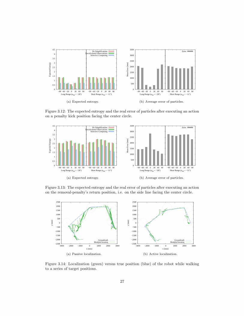
Since such simulations include considering all possible observations for all actionsfor a current belief state which is expressed with a number of particles, this calculationinvolves a significant computational complexity. Several approximations were considered,implemented (if practical), and evaluated for approximation quality and speed-up:
• Using clusters instead of separate particles for entropy calculation; neglects theparticle variations inside the cluster.
• Precomputing observations in look-up table; introduces discretization error.
• Precomputing the measurement probability for each possible pose and action deci-sion; not practical since the table size exceeds 100MB for sensible resolutions.
• Neglecting areas with low particle density.
The effects on estimation quality are visualized in figures 3.12 and 3.13. The resultingsystem has a average runtime of 4.2 ms on the Nao. Comparative results of the pre-sented approach against the previously used passive scanning are visualized in figures 3.14and 3.15 where the robot walked to a series of points.
This module has not been used in RoboCup 2010 nor 2011. The main reason hasbeen the change of the localization strategy described in section 3.3. There are also someadditional issues that need to be addressed. Since the underlying particle localizationdoes not take into account negative information the active vision approach tends to failin kidnapped robot scenarios where the belief state is absolutely wrong. In this casethe active vision decision is based on incorrect data and the supposedly optimal decisionmay look at areas without useful features. Since “not seeing anything” does not change
26
0
0.5
1
1.5
2
2.5
3
3.5
4
4.5
−90 −60 −30 0 30 60 90
Exp
ecte
d E
ntro
py
Long Range (utilt = −28°)
−90 −60 −30 0 30 60 90
Short Range (utilt = −11°)
No SimplificationsPrecalculated Observations
Selective Computing
(a) Expected entropy.
0
500
1000
1500
2000
2500
3000
3500
−90 −60 −30 0 30 60 90
Mea
n E
rror
[mm
]
Long Range (utilt = −28°)
−90 −60 −30 0 30 60 90
Short Range (utilt = −11°)
Error
(b) Average error of particles.
Figure 3.12: The expected entropy and the real error of particles after executing an actionon a penalty kick position facing the center circle.
0
0.5
1
1.5
2
2.5
3
3.5
4
4.5
−90 −60 −30 0 30 60 90
Exp
ecte
d E
ntro
py
Long Range (utilt = −28°)
−90 −60 −30 0 30 60 90
Short Range (utilt = −11°)
No SimplificationsPrecalculated Observations
Selective Computing
(a) Expected entropy.
0
500
1000
1500
2000
2500
3000
3500
−90 −60 −30 0 30 60 90
Mea
n E
rror
[mm
]
Long Range (utilt = −28°)
−90 −60 −30 0 30 60 90
Short Range (utilt = −11°)
Error
(b) Average error of particles.
Figure 3.13: The expected entropy and the real error of particles after executing an actionon the removal-penalty’s return position, i.e. on the side line facing the center circle.
−2500
−2000
−1500
−1000
−500
0
500
1000
1500
2000
2500
−3000 −2000 −1000 0 1000 2000 3000
y [m
m]
x [mm]
GroundtruthModeled location
(a) Passive localization.
−2500
−2000
−1500
−1000
−500
0
500
1000
1500
2000
2500
−3000 −2000 −1000 0 1000 2000 3000
y [m
m]
x [mm]
GroundtruthModeled location
(b) Active localization.
Figure 3.14: Localization (green) versus true position (blue) of the robot while walkingto a series of target positions.
27
0
500
1000
1500
2000
2500
3000
0 50 100 150 200 250
Dis
tanc
e E
rror
[mm
]
ActivePassive
0 10 20 30 40 50 60 70 80 90
0 50 100 150 200 250
Bea
ring
Err
or [°
]
Time [s]
ActivePassive
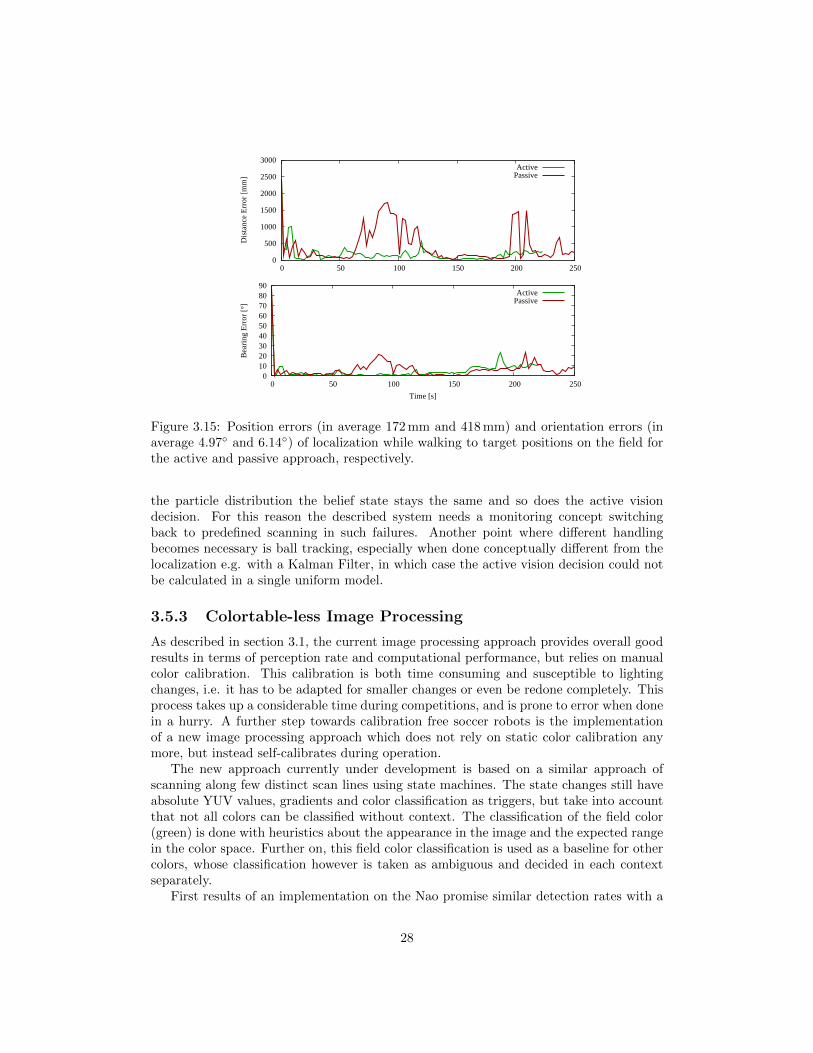
Figure 3.15: Position errors (in average 172 mm and 418 mm) and orientation errors (inaverage 4.97◦ and 6.14◦) of localization while walking to target positions on the field forthe active and passive approach, respectively.
the particle distribution the belief state stays the same and so does the active visiondecision. For this reason the described system needs a monitoring concept switchingback to predefined scanning in such failures. Another point where different handlingbecomes necessary is ball tracking, especially when done conceptually different from thelocalization e.g. with a Kalman Filter, in which case the active vision decision could notbe calculated in a single uniform model.
3.5.3 Colortable-less Image Processing
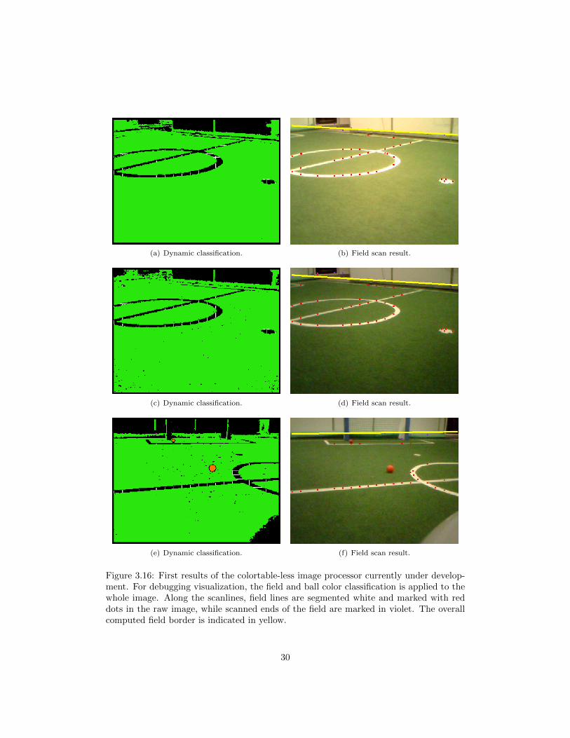
As described in section 3.1, the current image processing approach provides overall goodresults in terms of perception rate and computational performance, but relies on manualcolor calibration. This calibration is both time consuming and susceptible to lightingchanges, i.e. it has to be adapted for smaller changes or even be redone completely. Thisprocess takes up a considerable time during competitions, and is prone to error when donein a hurry. A further step towards calibration free soccer robots is the implementationof a new image processing approach which does not rely on static color calibration anymore, but instead self-calibrates during operation.
The new approach currently under development is based on a similar approach ofscanning along few distinct scan lines using state machines. The state changes still haveabsolute YUV values, gradients and color classification as triggers, but take into accountthat not all colors can be classified without context. The classification of the field color(green) is done with heuristics about the appearance in the image and the expected rangein the color space. Further on, this field color classification is used as a baseline for othercolors, whose classification however is taken as ambiguous and decided in each contextseparately.
First results of an implementation on the Nao promise similar detection rates with a
28

computational cost in the same range as the previous processing routines. Figure 3.16shows the classification and detection results of the current state of the implementation.
29
(a) Dynamic classification. (b) Field scan result.
(c) Dynamic classification. (d) Field scan result.
(e) Dynamic classification. (f) Field scan result.
Figure 3.16: First results of the colortable-less image processor currently under develop-ment. For debugging visualization, the field and ball color classification is applied to thewhole image. Along the scanlines, field lines are segmented white and marked with reddots in the raw image, while scanned ends of the field are marked in violet. The overallcomputed field border is indicated in yellow.
30
Chapter 4
Behavior
Nao Devils as well as previous Dortmund teams implemented behavior mostly by utilisingXABSL (Extensible Agent Behavior Specification Language). XABSL was developed inits original form in 2004 using XML syntax [21] in Darmstadt and Berlin and adaptedin 2005 to its current C-like syntax and a new ruby-based compiler by the MicrosoftHellhounds.
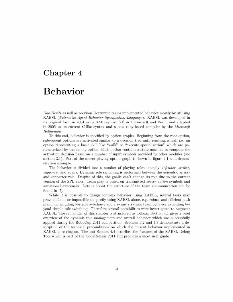
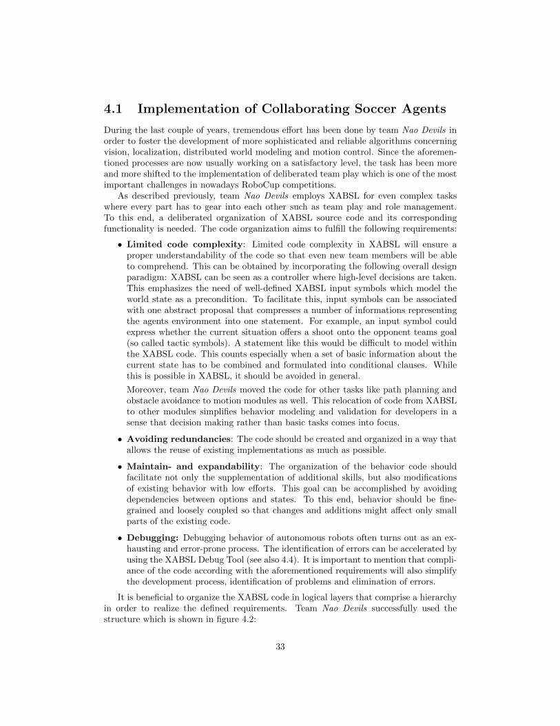
To this end, behavior is specified by option graphs. Beginning from the root option,subsequent options are activated similar to a decision tree until reaching a leaf, i.e. anoption representing a basic skill like “walk” or “execute special action” which are pa-rameterized by the calling option. Each option contains a state machine to compute theactivation decision based on a number of input symbols provided by other modules (seesection 3.1). Part of the soccer playing option graph is shown in figure 4.1 as a demon-stration example.
The behavior is divided into a number of playing roles, namely defender, striker,supporter and goalie. Dynamic role switching is performed between the defender, strikerand supporter role. Despite of this, the goalie can’t change its role due to the currentversion of the SPL rules. Team play is based on transmitted soccer action symbols andsituational awareness. Details about the structure of the team communication can befound in [7].
While it is possible to design complex behavior using XABSL, several tasks mayprove difficult or impossible to specify using XABSL alone, e.g. robust and efficient pathplanning including obstacle avoidance and also any strategic team behavior extending be-yond simple role switching. Therefore several possibilities were investigated to augmentXABSL: The remainder of this chapter is structured as follows: Section 4.1 gives a briefoverview of the dynamic role management and overall behavior which was successfullyapplied during the RoboCup 2011 competition. Sections 4.2 and 4.3 demonstrate a de-scription of the technical preconditions on which the current behavior implemented inXABSL is relying on. The last Section 4.4 describes the features of the XABSL DebugTool which is part of the CodeRelease 2011 and provides a short user guide.
31
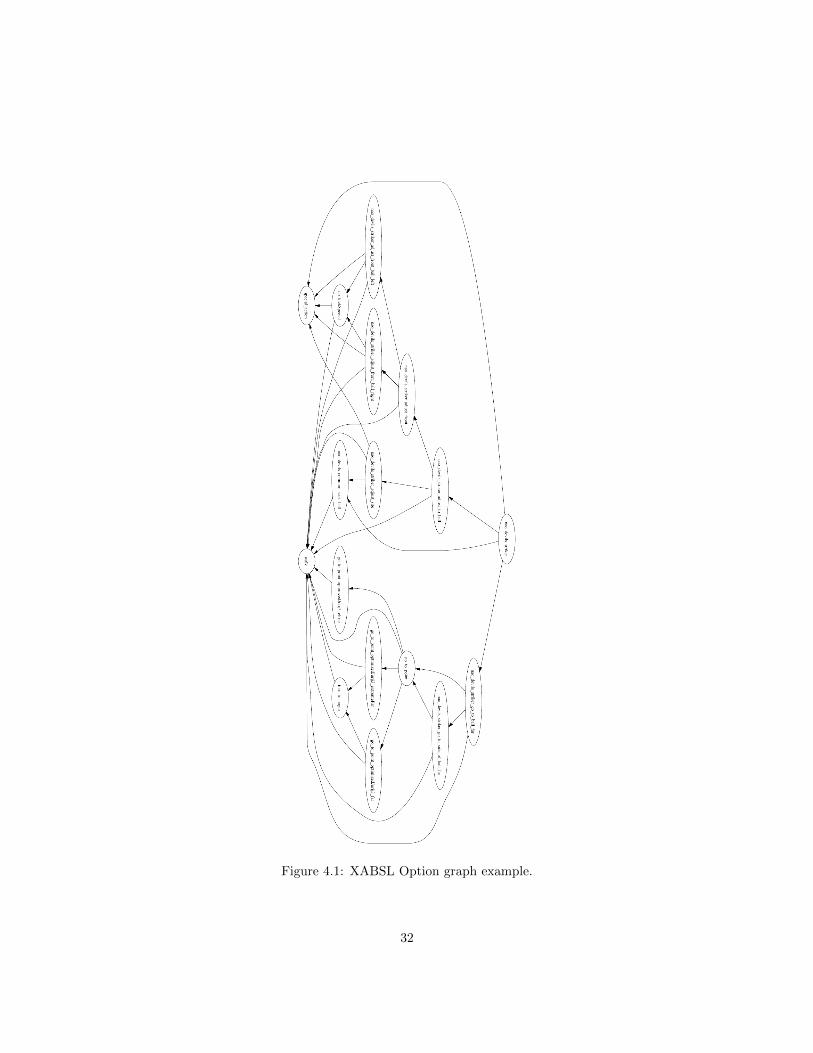
Figure 4.1: XABSL Option graph example.
32
4.1 Implementation of Collaborating Soccer Agents
During the last couple of years, tremendous effort has been done by team Nao Devils inorder to foster the development of more sophisticated and reliable algorithms concerningvision, localization, distributed world modeling and motion control. Since the aforemen-tioned processes are now usually working on a satisfactory level, the task has been moreand more shifted to the implementation of deliberated team play which is one of the mostimportant challenges in nowadays RoboCup competitions.
As described previously, team Nao Devils employs XABSL for even complex taskswhere every part has to gear into each other such as team play and role management.To this end, a deliberated organization of XABSL source code and its correspondingfunctionality is needed. The code organization aims to fulfill the following requirements:
• Limited code complexity: Limited code complexity in XABSL will ensure aproper understandability of the code so that even new team members will be ableto comprehend. This can be obtained by incorporating the following overall designparadigm: XABSL can be seen as a controller where high-level decisions are taken.This emphasizes the need of well-defined XABSL input symbols which model theworld state as a precondition. To facilitate this, input symbols can be associatedwith one abstract proposal that compresses a number of informations representingthe agents environment into one statement. For example, an input symbol couldexpress whether the current situation offers a shoot onto the opponent teams goal(so called tactic symbols). A statement like this would be difficult to model withinthe XABSL code. This counts especially when a set of basic information about thecurrent state has to be combined and formulated into conditional clauses. Whilethis is possible in XABSL, it should be avoided in general.
Moreover, team Nao Devils moved the code for other tasks like path planning andobstacle avoidance to motion modules as well. This relocation of code from XABSLto other modules simplifies behavior modeling and validation for developers in asense that decision making rather than basic tasks comes into focus.
• Avoiding redundancies: The code should be created and organized in a way thatallows the reuse of existing implementations as much as possible.
• Maintain- and expandability: The organization of the behavior code shouldfacilitate not only the supplementation of additional skills, but also modificationsof existing behavior with low efforts. This goal can be accomplished by avoidingdependencies between options and states. To this end, behavior should be fine-grained and loosely coupled so that changes and additions might affect only smallparts of the existing code.
• Debugging: Debugging behavior of autonomous robots often turns out as an ex-hausting and error-prone process. The identification of errors can be accelerated byusing the XABSL Debug Tool (see also 4.4). It is important to mention that compli-ance of the code according with the aforementioned requirements will also simplifythe development process, identification of problems and elimination of errors.
It is beneficial to organize the XABSL code in logical layers that comprise a hierarchyin order to realize the defined requirements. Team Nao Devils successfully used thestructure which is shown in figure 4.2:
33
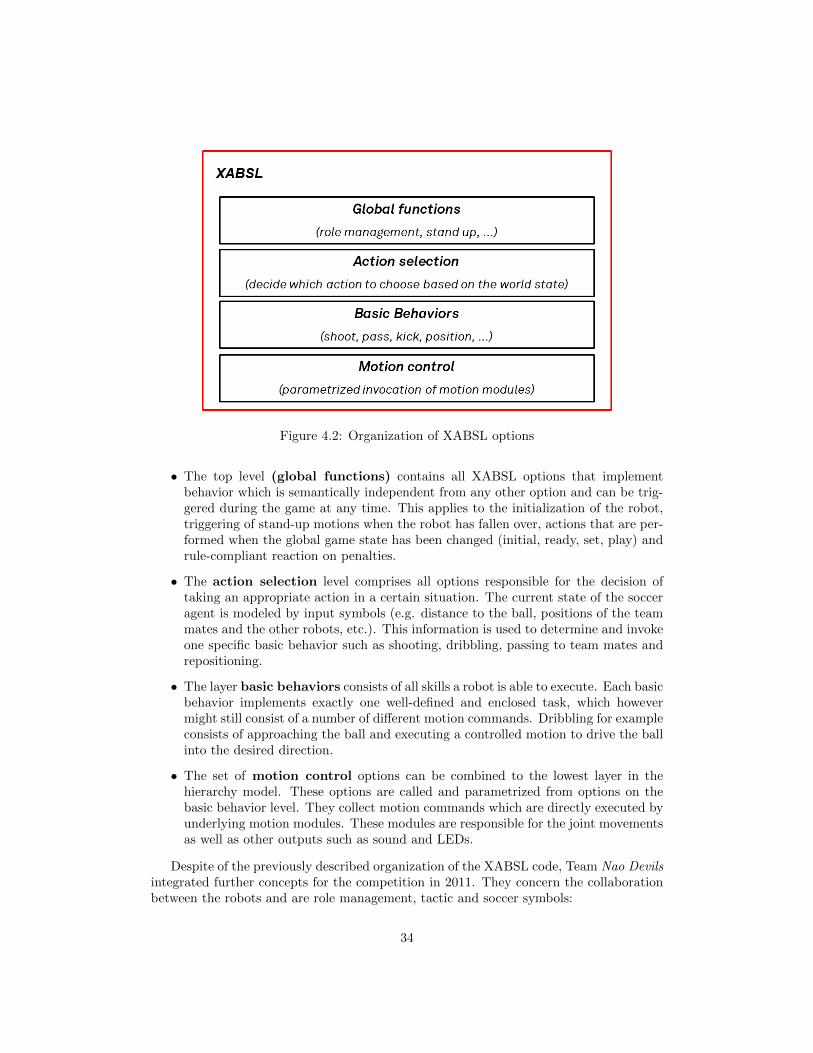
Figure 4.2: Organization of XABSL options
• The top level (global functions) contains all XABSL options that implementbehavior which is semantically independent from any other option and can be trig-gered during the game at any time. This applies to the initialization of the robot,triggering of stand-up motions when the robot has fallen over, actions that are per-formed when the global game state has been changed (initial, ready, set, play) andrule-compliant reaction on penalties.
• The action selection level comprises all options responsible for the decision oftaking an appropriate action in a certain situation. The current state of the socceragent is modeled by input symbols (e.g. distance to the ball, positions of the teammates and the other robots, etc.). This information is used to determine and invokeone specific basic behavior such as shooting, dribbling, passing to team mates andrepositioning.
• The layer basic behaviors consists of all skills a robot is able to execute. Each basicbehavior implements exactly one well-defined and enclosed task, which howevermight still consist of a number of different motion commands. Dribbling for exampleconsists of approaching the ball and executing a controlled motion to drive the ballinto the desired direction.
• The set of motion control options can be combined to the lowest layer in thehierarchy model. These options are called and parametrized from options on thebasic behavior level. They collect motion commands which are directly executed byunderlying motion modules. These modules are responsible for the joint movementsas well as other outputs such as sound and LEDs.
Despite of the previously described organization of the XABSL code, Team Nao Devilsintegrated further concepts for the competition in 2011. They concern the collaborationbetween the robots and are role management, tactic and soccer symbols:
34
• Changes in the role management: A major modification in the SPL was carriedout for 2011. The number of players increased from three to four players1. Thisforced major changes regarding dynamic role management between the agents. Inprevious years, three basic roles (keeper, supporter, striker) were defined and onewas assigned to each robot according to the position of the ball. Moreover, the rolesimplied different skills and, e.g. only the striker was able to kick the ball during thegame, and the robot which should kick the ball simply got assigned the striker role.
The current role management depends on the position of the team mates on thefield and whether several parts of the field are covered. The implication betweenrole and associated basic behaviors is dissolved.
• Employing tactic symbols: Deliberated tactic symbols contain information aboutthe current state of the game (e.g. whether an agent is the nearest to ball). Tocalculate this, additional input from the other agents is needed.
• Using soccer symbols: Soccer symbols show the action the robot is currentlyperforming, e.g. positioning, passing or kicking. This information is useful in teamplay since the other agents are able to apply supporting actions. Consider an agentwhich decides to pass the ball to a better positioned team mate: When the agentis passing the ball, the team mate could move his head to the direction where theball is expected to roll and is able to react quickly.
In summary, team Nao Devils worked mainly on the one hand on an appropriateXABSL code structure and on the other hand on mechanisms to improve team playaccording to the changed SPL rules in 2011, especially role management. Future workwill focus on the integration of machine learning algorithms concerning individual tasksto improve decision making.
4.2 Behavior Coordinate System
Past approaches to behavior planning of team Nao Devils were based on the robots currentview and thereby on the robot centric coordinate system. As described in chapter 2.1 thewalking engine applied by team Nao Devils is based on the concept of dynamic stability.Thus per definition it is impossible to stop the robot at any time during the execution ofa walking motion. This problem is coped with by introducing a preview phase containingthe next planned motion which has to be executed to ensure stability. Intuitively thiscorresponds to the inability to stop all motion while in the process of having one footlifted to bring forward when waling fast. In every case one has at least to execute thecurrent step to its end. But as a result a change of the walk request can only be executedwithin a given time, i.e. when the current swinging foot touches the ground and the nextfootstep is not yet planned into the current motion, thus resulting in a delay. This isespecially true for a complete stop, which is applied to position the robot next to theball. If a behavior is written to only set the target speed to zero the moment the targetposition is reached, the robot tends to overshoot and is likely to stumble against the ball.
In the past this problem was dealt with by stopping the robot some time beforeactually reaching the ball. But since the distance traveled after the stopping command is
1http://www.tzi.de/spl/pub/Website/Downloads/Rules2011.pdf
35
given differs depending on the speed and currently executed motion of the robot, findingthe right distance was a matter of time consuming manual tuning of the behavior andstill resulted in suboptimal results. Since XABSL itself does not address this problem, itis solved by introducing a new coordinate system, called after preview, centered on theexpected future robot position. Actually this coordinate system is not related to a fixedtime interval in the future, but rather to a dynamic offset depending on the executedmotion or walking phase, which might also be zero in case of statically stable motionswhich can be interrupted at any time.
Consequently also the representations available to the XABSL behavior module are nolonger the direct localization and tracking outputs, but those are transformed to the afterpreview coordinate system. This allows the behavior to make decisions based on the exactfuture state of the robot at which those behavior decisions actually have an impact. Allintermediate actions till this point will be executed independent of the current decision,so now the decisions will be based on the correct environmental circumstances on whichthis decision will be acting upon, resulting in more precise and reactive behavior planning.
When visualizing the corresponding representations (marked by “...AfterPreview”) inSimRobot, the origin for drawing first needs to be set using the following command:
vfd worldState origin:RobotPoseAfterPreview
4.3 GoTo Motion Command
The motion commands used in previous years till RoboCup 2009 have been based ondesired speed vectors which were updated with every behavior execution. This mode ofcontrol dates back to the AIBOs which could be controlled like omnidirectional vehicles.Additionally for an AIBO it was sufficient to walk straight to the ball to grab and turn withit. For humanoid robots however the the omnidirectional characteristic of the walkinggeneration is much less distinct, and at the same time a target position close to the ball hasto be reached with a certain target orientation which increases the difficulty for trajectorycontrol. While it is possible and also commonly done to generate omnidirectional walkingpatterns with the walking engine described in section 2.1, for a humanoid robot suchas the Nao it is far more convenient to walk straight than it is to walk sideways. Thisis reflected in the possible walking speeds in each direction. Generating smooth pathtrajectories following the characteristics optimal for those described walking capabilitiesis obviously not possible in an intuitive way using a state-based behavior descriptionlanguage such as XABSL.
To overcome those limitations and ultimately to achieve more precision and speedin positioning close to the ball, a more advanced approach to path planning has beendone for the Nao Devils’ robots for RoboCup 2010. The utilized Dortmund WalkingEngine is based on foot step planning (see section 2.1). In 2010, a basic behavior hasbeen introduced to XABSL allowing the trajectory planning to be done by the walkingengine which has much better control and feedback about the executed motion. Themotion request has been adapted accordingly to accept a target position and orientationand different XABSL go to commands have been implemented to cover common motiontasks.
In the current implementation of this basic behavior a target position relative to thecurrent behavior reference frame (compare section 4.2) can be specified. Compared to the
36

version from 2010, especially since there are now four robots on the field for each team,it was necessary to include some kind of obstacle avoidance into our path planning.
Due to the improvements in our world state model (see 3.4) a predictive path planningwas made possible. Still, the world around the robot will be changing in a way that ishard to predict, therefore we decided against the planning of a complete path and ratheruse a potential field, which also does not take away much of our already limited computingpower.
With the target position coming from our behavior as a positive potential, the poten-tial field is created. Then Robots from the Robotmap, the goalposts, the ball and, if therobot is a field player, the own penalty area are added as negative potentials.
The potential of robots is, using a gaussian distribution, modeled as an ellipse, whichlonger axis is aligned parallel to the line that connects the robot with its current tar-get. This enforces a straighter path around the obstacle than it would be possible witha circular modeling of the other robots, resulting in a overall higher speed around anobstacle.
Within this potential field a path is constructed by using the gradient at the robot’sposition, moving a fixed length into that direction and repeating the process several times,or until the destination is reached.
Along this path, a smoothed trajectory for the PatternGenerator (see section 2.1) iscreated, that fulfills the following criteria :
• move as fast as possible towards the target,
• keep the target and obstacles in sight and
• keep the motion as smooth as possible.
A potential field itself, if used for path planning, has some drawbacks, if only theresulting force is used as the direction for the robot to walk, especially the existence oflocal minima and the possibilty of flickering trajectories.
The first problem is solved by simply merging two obstacles, that could create a localminima into one bigger obstacle. The second problem is implicitly solved by constructingthe path and smoothing out the actual motion after that.
One of the remaining problems is the possibilty that the robot switches the side onthat he wants to avoid the obstacle, slowing down the whole evasion process. Anotherproblem is the inability to avoid large walls of obstacles since the path planning doesoperate only locally.
Despite that, in real game situations the time to reach the robots destination whenfaced with osbtacles could be reduced significantly.
The path through the potential field can be visualized using SimRobot. After settingthe origin for drawing to the behavior coordinate system as described in section 4.2, thefollowing command will display the corresponding drawing as can be seen in figure 4.3:
vfd worldState representation:Path
4.4 Debug Tool
Debugging programmed code is essential to identify flaws and finding solutions to errors.This is not only true for the code of the robotic framework, but also for the behavior
37
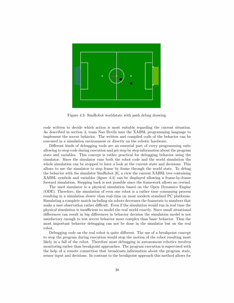
Figure 4.3: SimRobot worldstate with path debug drawing.
code written to decide which action is most suitable regarding the current situation.As described in section 4, team Nao Devils uses the XABSL programming language toimplement the soccer behavior. The written and compiled code of the behavior can beexecuted in a simulation environment or directly on the robotic hardware.
Different kinds of debugging tools are an essential part of every programming suiteallowing to stop code during execution and get step by step information about the programstate and variables. This concept is rather practical for debugging behavior using thesimulator. Since the simulator runs both the robot code and the world simulation thewhole simulation can be stopped to have a look at the current state and decisions. Thisallows to use the simulator to step frame by frame through the world state. To debugthe behavior with the simulator SimRobot [8], a view the current XABSL tree containingXABSL symbols and variables (figure 4.4) can be displayed allowing a frame-by-frameforward simulation. Stepping back is not possible since the framework allows no rewind.
The used simulator is a physical simulation based on the Open Dynamics Engine(ODE). Therefore, the simulation of even one robot is a rather time consuming processresulting in a simulation slower than real-time on most modern standard PC platforms.Simulating a complete match including six robots decreases the framerate to numbers thatmake a user observation rather difficult. Even if the simulation would run in real time thephysical simulation is insufficient to model the real world exactly. Since small situationaldifferences can result in big differences in behavior decision the simulation model is notsatisfactory enough to test soccer behavior more complex than basic behavior. Thus themost important behavior debugging can not be done in the simulator but on the realrobot.
Debugging code on the real robot is quite different. The use of a breakpoint conceptto stop the program during execution would stop the motion of the robot resulting mostlikely in a fall of the robot. Therefore most debugging in autonomous robotics involvesmonitoring rather than breakpoint approaches. The program execution is supervised withthe help of a remote connection that broadcasts information about the program state,sensor input and decisions. In contrast to the breakpoint approach this method allows for
38

Figure 4.4: Example of a XABSL tree.
a debugging in real game situations involving other autonomous robots but is prohibitedduring tournament game play. Unfortunately the nature of the supervision process resultsin a delay of information. Therefore the supervision cannot be matched exactly with thecurrent field situation. In addition the broadcast connection results in an disturbance ofthe the normal code execution. In general the disturbance is minor in scope but can resultin timing problems. The result would be a stuttering of the robot which changes the statethat should only be monitored. Especially for debugging of robot behavior supervision ofthe written code is a rather inadequate solution.
Since execution directly onto the robot is of special interest for behavior developmentteam Nao Devils developed a tool allowing a different debugging concept combining theconvenience of simulator debugging with code testing on the real robot. The concept isbased on logging each behavior decision during the execution. To allow a later analysisof the logged data the corresponding sensor information is also stored in addition to eachdecision. Since the complete sensor information, including the camera pictures, wouldresult in an unmanageable amount of data, only the resulting information about theworld model are saved.
With this stored data a playback of all behavior decisions and a debugging of decisionson given data can be done. But an analysis of the world model is not possible, since onlythe modeled gamestate is stored and cannot be compared with reality. But to allow eventhat comparison a video camera can be used to record the real gamestate in a movie file.
Based in these concepts team Nao Devils developed a tool with following features:
• The robot logs its internal state machine, the required symbols and hardware com-mands (motion, LED-Requests etc.) once per frame.
• A graphical user interface allows for an easy reading of the logfile and shows theinput/output symbols and current XABSL state tree.
39
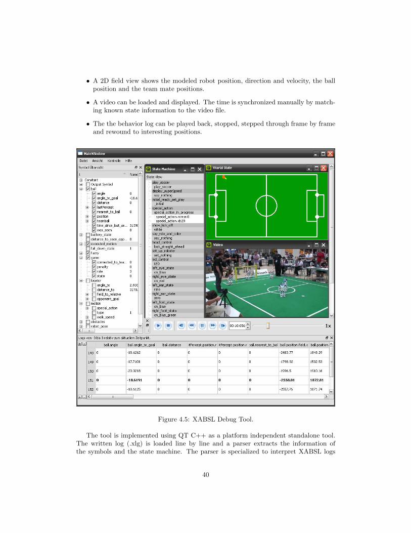
• A 2D field view shows the modeled robot position, direction and velocity, the ballposition and the team mate positions.
• A video can be loaded and displayed. The time is synchronized manually by match-ing known state information to the video file.
• The the behavior log can be played back, stopped, stepped through frame by frameand rewound to interesting positions.
Figure 4.5: XABSL Debug Tool.
The tool is implemented using QT C++ as a platform independent standalone tool.The written log (.xlg) is loaded line by line and a parser extracts the information ofthe symbols and the state machine. The parser is specialized to interpret XABSL logs
40

but due to clearly defined interfaces between the interpreter and the different widgetsan adaptation to another behavior language would be possibly by changing the parser.Additional debug views specialized for other description languages can also be addedeasily.
The progress bar allows an intuitive navigation within the log file. The current frameinformation is shown using the following widgets (see figure 4.5):
• Input/output Symbols-Treeview Widget: Displays an overview with all loggedsymbols and their values represented in a tree. It’s possible to select specific symbolsto display more detailed information.
• Detailed Symbols Widget: All symbols selected in the Symbols-Tree-View areshown as a table here, so that the user has a quick overview about the neededsymbols. The columns represent the symbol names, the rows represent differentframes. By highlighting current frame the user can see the chronological historyof the symbols. This is useful, if the user wants to judge the stability of a givensymbol.
• Woldstate Widget: A 2D-Field is painted, displaying the current modeled robotposition, direction, velocity and the latest ball position. This overview allows theuser to judge the internal robot world model and compare it to the reality repre-sented by the video file.
• Video Widget: Display of the video file synchronized to the internal robot state.
• Control Widget: The user can navigate within the logfile including jump for-ward, back step by step, play slow-motion etc.
• Statemachine Widget: This Widget shows the current option-state path.
All this is designed to enable a behavior designer to replay all the states and analyzethe decisions a robot made. It is therefore easy to find out,
• whether a decision was based on a false perception: If the robot would have correctlyseen a certain feature, it would have behaved correctly. This kind of error resultsfrom either a false perception or wrong interpretation and modeling.
• whether the decision was based on false decisions made on correct knowledge: Theuser observes a gamestate which resulted in an undesired decision. If the internalworld model matches the real world the wrong decision is a result of a decision erroror a coding bug.
The tool is still in an early state of development missing features such as synchronizinglog files of different robots to debug team decisions. But still the debugging tool has provenhelpful in replaying gamestate decisions and allowing expert programmers to judge anddebug errors thereby improving the written XABSL code. The most useful informationwas thereby gained from actual tournament games which were otherwise impossible tosupervise due to the given rules.
41
Chapter 5
Conclusion and Outlook
The Nao Devils Dortmund is a team from the TU Dortmund University with roots inseveral other teams which have competed in RoboCup competitions over the last years.This team report covered a short overview of the main ideas and concepts that wereemployed and successfully used in RoboCup2011 where the Nao Devils were able to takethe 2nd place with 36 obtained goals in 9 games.
One major change in the SPL rules this year was the increase of the number of playersper team by one. This greatly affected the development of team behavior with specialrespect to the role management. To this end, the role management has been completelyrewritten from the scratch. It contains a paradigm change from a simple, classical rolemanagement with three possible roles (striker, supporter and goalie) and their associatedbehavior to a more sophisticated zone-depending role management that makes team playmore flexible. Experience from last years competition has also revealed that a lot oftackling is involved during games. This emphasised the need of a deliberared strategy todeal with very situations. The Nao Devils were successfully able to speed-up basic taskssuch as approaching and kicking the ball by improving underlying Motion and Cognitionprocesses with respect to precision and stability.
Another major challenge was the integration of visual robot detection that comple-mented the awareness of opponent robots. This allowed the use of key aspects of thedistributed world modeling approach that was briefly proposed. This helped to enhancestrategical positioning, advanced tactical play of the robots and team ball localization. Inaddition part of the focus will still lie on motion generation, refining and extending theexisting walking algorithms and further develop the path planning and motion execution.
42
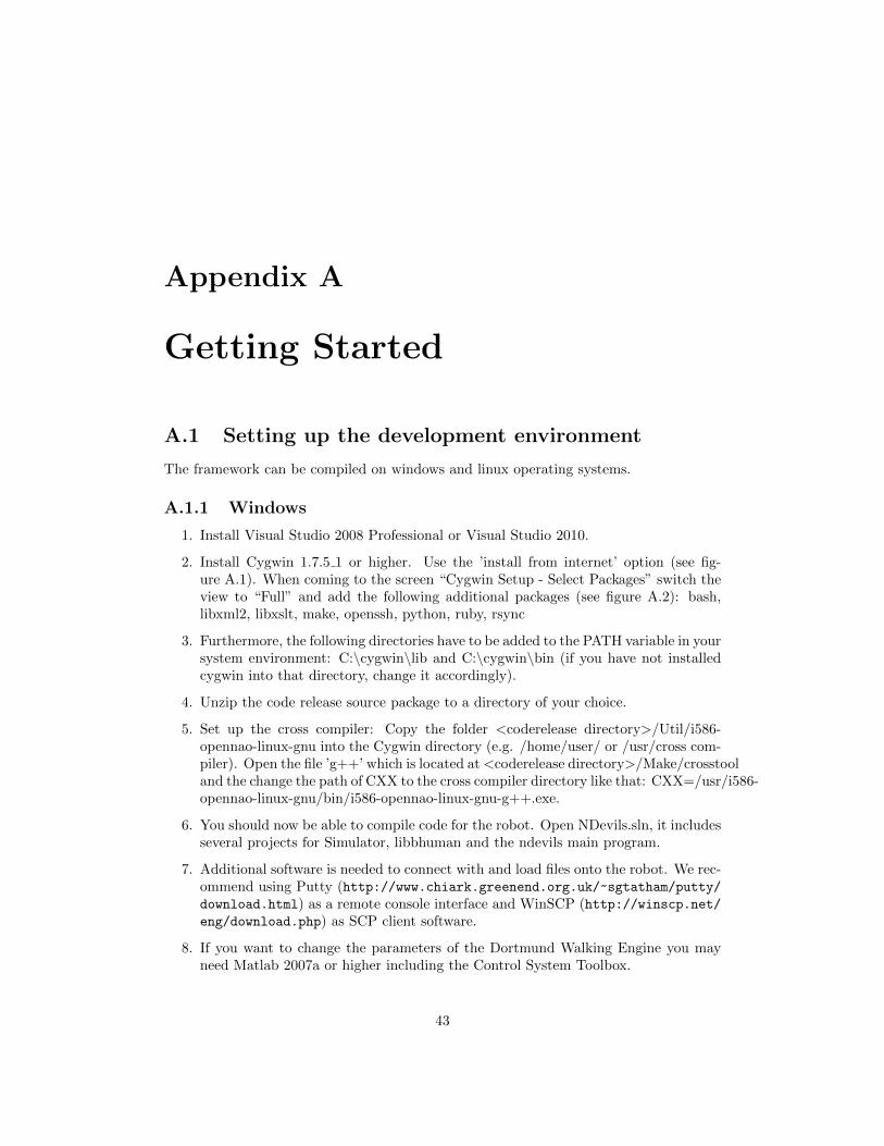
Appendix A
Getting Started
A.1 Setting up the development environment
The framework can be compiled on windows and linux operating systems.
A.1.1 Windows
1. Install Visual Studio 2008 Professional or Visual Studio 2010.
2. Install Cygwin 1.7.5 1 or higher. Use the ’install from internet’ option (see fig-ure A.1). When coming to the screen “Cygwin Setup - Select Packages” switch theview to “Full” and add the following additional packages (see figure A.2): bash,libxml2, libxslt, make, openssh, python, ruby, rsync
3. Furthermore, the following directories have to be added to the PATH variable in yoursystem environment: C:\cygwin\lib and C:\cygwin\bin (if you have not installedcygwin into that directory, change it accordingly).
4. Unzip the code release source package to a directory of your choice.
5. Set up the cross compiler: Copy the folder <coderelease directory>/Util/i586-opennao-linux-gnu into the Cygwin directory (e.g. /home/user/ or /usr/cross com-piler). Open the file ’g++’ which is located at <coderelease directory>/Make/crosstooland the change the path of CXX to the cross compiler directory like that: CXX=/usr/i586-opennao-linux-gnu/bin/i586-opennao-linux-gnu-g++.exe.
6. You should now be able to compile code for the robot. Open NDevils.sln, it includesseveral projects for Simulator, libbhuman and the ndevils main program.
7. Additional software is needed to connect with and load files onto the robot. We rec-ommend using Putty (http://www.chiark.greenend.org.uk/~sgtatham/putty/download.html) as a remote console interface and WinSCP (http://winscp.net/eng/download.php) as SCP client software.
8. If you want to change the parameters of the Dortmund Walking Engine you mayneed Matlab 2007a or higher including the Control System Toolbox.
43

Figure A.1: Cygwin Setup.
Figure A.2: Installing additional Cygwin packages.
44

A.1.2 Linux
You can use any Linux distribution as well to compile the robot code. Simply unzip thesource package into a directory of your choice. Like in the windows setup, bash, ruby, gnumake, ssh, rsync, an xslt parser software and python have to be installed. Adapt the g++file as described at the windows section. Switch to the Make directory of the codereleasedirectory and run make (e.g. with the parameters <Nao|libbhuman|Behavior|SpecialActions>Config=<Debug|Release>). The Linux makefiles for each project are generated automat-ically with zbuild. Note that the Simulator can not be compiled under Linux Platforms.
A.1.3 Build configurations
Our code release consists of two different build configurations, RELEASE and DEBUG.The DEBUG configuration makes it possible to connect with SimRobot. The actualstate of the robot can be shown and modified. Running the robot with the DEBUGconfiguration will result in frame drops which means that the Cognition and Motionthread can not be executed stable at 33 Hz and 100 Hz respectively. Use RELEASEwhen high performance is required. The RELEASE configuration ignores every sourcewhich is needed for debugging except Profiling features.
A.2 Setting up the robot
Setting up the robot to run the newly compiled code consists of several steps. The memorysticks of the Nao V3+ robots needs to be flashed once for each robot as described in thefollowing section. Each time a different user works with a robot he needs to set up hisconfiguration (see section A.2.2). Section A.2.3 and A.2.4 finally describe how to run anddebug code on the robot.
A.2.1 Preparing the memory stick
Linux is required in order to set up a new stick for the Nao robot. This only needs to bedone once per robot.
1. Download opennao-robocup-1.6.13-nao-geode.ext3.gz from the Aldebaran websiteand copy it into /images of the Install folder (or use -i ¡image.ext3¿).
2. Plug the flashstick in your pc USB socket.
3. Run ./flash-and-install.sh as an administrator, e.g.: sudo ./flash-and-install.sh un-der Ubuntu.
The script uses Connman to connect the wireless LAN. Therefore, a few more stepsare needed to configure the wireless connection:
1. After flash-and-install.sh is executed, the Nao should be booted with the new USB-stick and a connected network cable.
2. Press the chest button of the Nao in order to get the current IP of the robot.
45
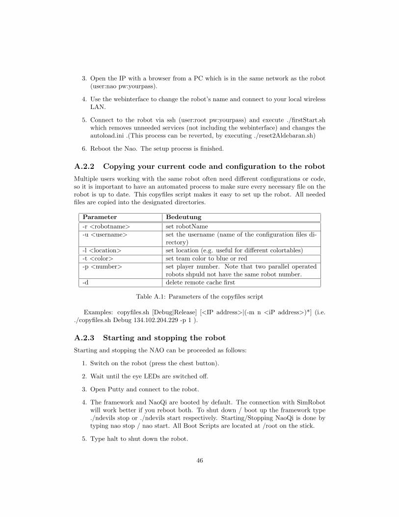
3. Open the IP with a browser from a PC which is in the same network as the robot(user:nao pw:yourpass).
4. Use the webinterface to change the robot’s name and connect to your local wirelessLAN.
5. Connect to the robot via ssh (user:root pw:yourpass) and execute ./firstStart.shwhich removes unneeded services (not including the webinterface) and changes theautoload.ini .(This process can be reverted, by executing ./reset2Aldebaran.sh)
6. Reboot the Nao. The setup process is finished.
A.2.2 Copying your current code and configuration to the robot
Multiple users working with the same robot often need different configurations or code,so it is important to have an automated process to make sure every necessary file on therobot is up to date. This copyfiles script makes it easy to set up the robot. All neededfiles are copied into the designated directories.
Parameter Bedeutung
-r <robotname> set robotName-u <username> set the username (name of the configuration files di-
rectory)-l <location> set location (e.g. useful for different colortables)-t <color> set team color to blue or red-p <number> set player number. Note that two parallel operated
robots shpuld not have the same robot number.-d delete remote cache first
Table A.1: Parameters of the copyfiles script
Examples: copyfiles.sh [Debug|Release] [<IP address>|(-m n <iP address>)*] (i.e../copyfiles.sh Debug 134.102.204.229 -p 1 ).
A.2.3 Starting and stopping the robot
Starting and stopping the NAO can be proceeded as follows:
1. Switch on the robot (press the chest button).
2. Wait until the eye LEDs are switched off.
3. Open Putty and connect to the robot.
4. The framework and NaoQi are booted by default. The connection with SimRobotwill work better if you reboot both. To shut down / boot up the framework type./ndevils stop or ./ndevils start respectively. Starting/Stopping NaoQi is done bytyping nao stop / nao start. All Boot Scripts are located at /root on the stick.
5. Type halt to shut down the robot.
46

A.2.4 How to connect with the robot and debug
SimRobot can be used to connect with the robot. Simply, you have to modify the fileconnect.con which is located under <Coderelease>/Config/Scenes. Replace the IP ad-dress in the command sc Remote 192.168.1.2. Boot up SimRobot and open the SceneRemoteRobot.con.The following table shows a set of basic Simulator commands which are useful for debug-ging purposes.
Parameter Description
log start starts recording a logfile.log stop stops recording a logfile.log save <filename> save the actual log to a specified file. The saved
file is located at <Coderelease>/Config/Logs.vi image raw Transmits uncompressed raw images from the
robot to the Simulator.vid raw representation:<class>: <element>
draws recognized elements on the image view. Itis useful in order to determine if the robot detectsballs, goal posts etc.
vf worldState creates a worldState view on which additional 2Dinformation can be drawn
vfd worldState representation:<class>: <element>
draws elements on the worldState view. This canbe e.g. ball percepts, robot poses etc.
Table A.2: Parameters of the copyfiles script
A detailed description of SimRobot and its commands can be found in [7] chapter 8.Please consult the manual for creating a colortable as well.
A.2.5 Using the XABSL Debug Tool
The XABSL debug logging can be activated in the ’behavior.cfg’ file which can be foundon the robot under ’[your Config]/Locations/[your location]’. Now create the directoryfor the log(s) : the debug tool expects a ’Logs’ folder in your config folder on the robot.As the last step add logging for your XABSL symbols by editing the respective .cpp fileas following :
• For static symbols (e.g. constant symbols or field symbols) add a methoddebugLogStatics() to your c++ symbol files (see Listing A.1).
• For every-frame-updated symbols add a debugLog() and debugLogPrintTitle()method to your c++ smybol files (see Listing A.2).
47
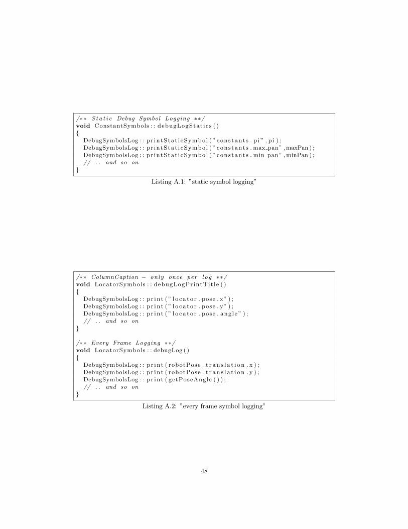
/∗∗ S t a t i c Debug Symbol Logging ∗∗/void ConstantSymbols : : debugLogStat ics ( ){
DebugSymbolsLog : : pr intStat i cSymbol ( ” cons tant s . p i ” , p i ) ;DebugSymbolsLog : : pr intStat i cSymbol ( ” cons tant s . max pan” ,maxPan ) ;DebugSymbolsLog : : pr intStat i cSymbol ( ” cons tant s . min pan” ,minPan ) ;// . . and so on
}
Listing A.1: ”static symbol logging”
/∗∗ ColumnCaption − only once per l o g ∗∗/void LocatorSymbols : : debugLogPrintTit le ( ){
DebugSymbolsLog : : p r i n t ( ” l o c a t o r . pose . x” ) ;DebugSymbolsLog : : p r i n t ( ” l o c a t o r . pose . y” ) ;DebugSymbolsLog : : p r i n t ( ” l o c a t o r . pose . ang le ” ) ;// . . and so on
}
/∗∗ Every Frame Logging ∗∗/void LocatorSymbols : : debugLog ( ){
DebugSymbolsLog : : p r i n t ( robotPose . t r a n s l a t i o n . x ) ;DebugSymbolsLog : : p r i n t ( robotPose . t r a n s l a t i o n . y ) ;DebugSymbolsLog : : p r i n t ( getPoseAngle ( ) ) ;// . . and so on
}
Listing A.2: ”every frame symbol logging”
48
Appendix B
Framework
The German Team Framework [6] was chosen to be the basis for all code being written.Since both B-Human and the Microsoft Hellhounds were using variations or predecessorsof this framework large amounts of already available modules (e.g. ImageProcessing,BallModelling) could be ported rapidly and with ease. A more detailed description of themost recent version of this framework can be found in [7].
The framework itself is based on a modular structure. A module can be seen as a pos-sible solution for a certain task. This could either be self-localization, image-processingor something else. Modules can be exchanged at runtime which simplifies the compar-ison and evaluation of different solutions for a specific task. The coupling between themodules is created by so called representations which can either be required or providedby a specific module. The modules itself are grouped in so called processes. For nowthere exist only two processes. The motion process encapsulates all modules concerningthe generation of motion trajectories. This includes for example the WalkingEngine orthe SpecialActionEngine. The cognition process however contains modules for imagepro-cessing, localization and bahavior control. The data exchange between the frameworkprocesses is done via means of Inter-Process Communication. For now the data is ex-changed via a shared-memory system.
B.1 Modules
As mentioned before modules are the essential elements of the framework. A moduleconsists of three parts:
• the module interface
• its actual implementation
• a statement that allows to instantiate the module.
The module interface defines the name of the module, the representations required by themodule to operate and the representations it provides/modifies. This interface basicallycreates a basis for the actual implementation. An example module definition can be seenin listing B.1.
49

/∗∗ Module De f i n i t i on ∗∗/MODULE(DemoImageProcessor )
/∗∗ Needs Image Representa t ion ∗∗/REQUIRES( Image )/∗∗ Needs CameraMatrix Representa t ion ∗∗/REQUIRES(CameraMatrix )/∗∗ Needs FrameInfo Representa t ion ∗∗/REQUIRES( FrameInfo )/∗∗ Provides Bal lModel Representa t ion ∗∗/PROVIDES( BallModel )/∗∗ Provides PointsPercept Representa t ionwi th debugg ing c a p a b i l i t i e s ∗∗/PROVIDESWITHMODIFY AND OUTPUT( PointsPercept )
ENDMODULE
Listing B.1: ”Example Module Definition”
The actual implementation of the module is done in a class derived from the moduledefinition. The implementation has class-wide read-only access to the required repre-sentations. For each provided representation an update method with a reference to therepresentation as parameter has to be implemented ( e.g. void update(BallModel&)).
At last the module needs to be instantiated, this is done via a call to MAKE MODULE,which takes a category as its second parameter allowing to specify a category for debuggingpurposes. Listing B.2 shows as an example how to implement an module from the previousmodule definition.
B.2 Representations
Representations are used to exchange data between modules. They are essentially lightweight data structures, which only contain the necessary information needed and providedby a module. Additionally all representations must implement an serialization interfacecalled Streamable which on the one hand enables the exchange of data between frameworkprocesses and on the other hand is used for debugging purposes. Listing B.3 shows anexample Representation.
B.3 Origin of Modules
The code released together with this report is based on the most recent version of theGermanTeam framework originating from the code release by BHuman in 2009. Asdescribed earlier this is used due to the Nao Devils’ history both in the GermanTeam andthe BreDoBrothers. Most of the code related to infrastructure and framework-internalsis left unchanged. The modules containing cognition and motion algorithms however aremostly developed in Dortmund. An overview about the origins of these modules is givenin tables B.1 and B.2. Infrastructure modules, e.g. those containing the code to obtainimages and sensor readings or to read or write joint angles, are omitted in those tables.
50

/∗∗ Module Implementation ∗∗//∗∗ Implement DemoImageProcessor de r i v ed from Module De f i n i t i on ∗∗/class DemoImageProcessor : public DemoImageProcessorBase{
void update ( BallModel& pBallModel ){
// update the Bal lModel r e p r e s en t a t i on}void update ( PointsPercept& pPointsPercept ){
// update the PointsPecept r e p r e s en t a t i on}
} ;
/∗∗ Module I n s t a n t i a t i o n ∗∗//∗∗ I n s t a n t i a t e Module DemoImageProcessor
in ca tegory ” ImageProcessing ” ∗∗/MAKEMODULE(DemoImageProcessor , ImageProcess ing )
Listing B.2: ”Example module implementation and instantiation”
Modules with origin in “Bremen” are kept from the BHuman code release for variousreasons, because they were either kept from the BreDoBrothers cooperation (e.g. the Par-ticleFilterBallLocator), equivalent in function (as the RobotModelProvider [7] comparedto the EgoModelProvider [22]) or providing new functionality (as the ObstacleModel-Provider for the sonar filtering). Origin “Dortmund” indicates Nao Devils’ developmentsor late Microsoft Hellhounds code. “GermanTeam” marks those parts of the code whichwere not necessarily in this exact modul form, but nevertheless date back to 2005 or beforeand were developed together by the GermanTeam of which both Bremen and Dortmundhave been members.
51
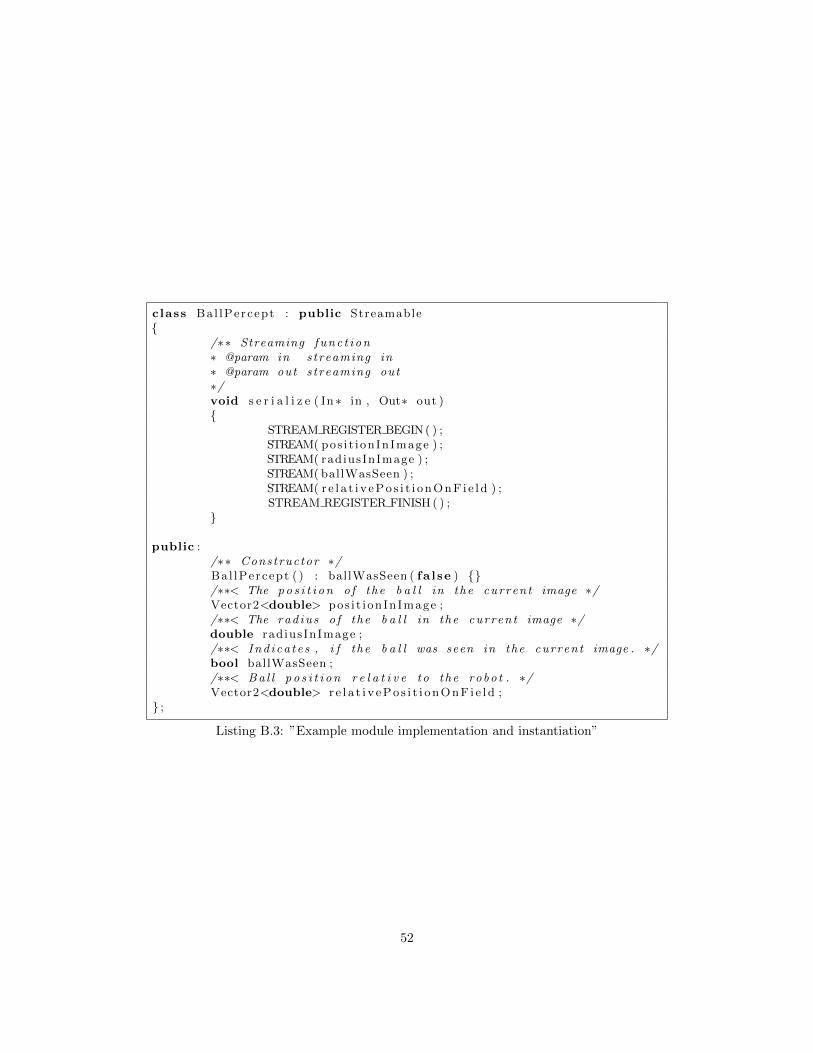
class Bal lPercept : public Streamable{
/∗∗ Streaming func t i on∗ @param in streaming in∗ @param out streaming out∗/void s e r i a l i z e ( In∗ in , Out∗ out ){
STREAM REGISTER BEGIN( ) ;STREAM( pos i t i onInImage ) ;STREAM( radiusInImage ) ;STREAM( ballWasSeen ) ;STREAM( r e l a t i v ePo s i t i onOnF i e l d ) ;STREAM REGISTER FINISH ( ) ;
}
public :/∗∗ Constructor ∗/Bal lPercept ( ) : ballWasSeen ( fa l se ) {}/∗∗< The po s i t i o n o f the b a l l in the curren t image ∗/Vector2<double> pos i t i onInImage ;/∗∗< The rad ius o f the b a l l in the curren t image ∗/double radiusInImage ;/∗∗< Ind i ca t e s , i f the b a l l was seen in the current image . ∗/bool ballWasSeen ;/∗∗< Ba l l p o s i t i o n r e l a t i v e to the robo t . ∗/Vector2<double> r e l a t i v ePo s i t i onOnF i e l d ;
} ;
Listing B.3: ”Example module implementation and instantiation”
52
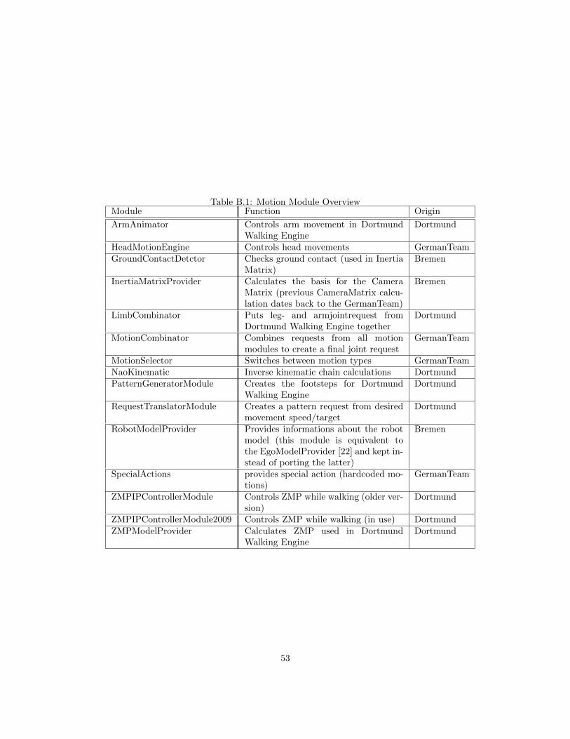
Table B.1: Motion Module OverviewModule Function Origin
ArmAnimator Controls arm movement in DortmundWalking Engine
Dortmund
HeadMotionEngine Controls head movements GermanTeamGroundContactDetctor Checks ground contact (used in Inertia
Matrix)Bremen
InertiaMatrixProvider Calculates the basis for the CameraMatrix (previous CameraMatrix calcu-lation dates back to the GermanTeam)
Bremen
LimbCombinator Puts leg- and armjointrequest fromDortmund Walking Engine together
Dortmund
MotionCombinator Combines requests from all motionmodules to create a final joint request
GermanTeam
MotionSelector Switches between motion types GermanTeamNaoKinematic Inverse kinematic chain calculations DortmundPatternGeneratorModule Creates the footsteps for Dortmund
Walking EngineDortmund
RequestTranslatorModule Creates a pattern request from desiredmovement speed/target
Dortmund
RobotModelProvider Provides informations about the robotmodel (this module is equivalent tothe EgoModelProvider [22] and kept in-stead of porting the latter)
Bremen
SpecialActions provides special action (hardcoded mo-tions)
GermanTeam
ZMPIPControllerModule Controls ZMP while walking (older ver-sion)
Dortmund
ZMPIPControllerModule2009 Controls ZMP while walking (in use) DortmundZMPModelProvider Calculates ZMP used in Dortmund
Walking EngineDortmund
53
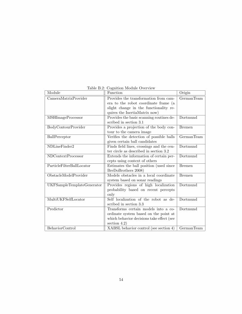
Table B.2: Cognition Module OverviewModule Function Origin
CameraMatrixProvider Provides the transformation from cam-era to the robot coordinate frame (aslight change in the functionality re-quires the InertiaMatrix now)
GermanTeam
MSHImageProcessor Provides the basic scanning routines de-scribed in section 3.1
Dortmund
BodyContourProvider Provides a projection of the body con-tour to the camera image
Bremen
BallPerceptor Verifies the detection of possible ballsgiven certain ball candidates
GermanTeam
NDLineFinder2 Finds field lines, crossings and the cen-ter circle as described in section 3.2
Dortmund
NDContextProcessor Extends the information of certain per-cepts using context of others
Dortmund
ParticleFilterBallLocator Estimates the ball position (used sinceBreDoBrothers 2008)
Bremen
ObstacleModelProvider Models obstacles in a local coordinatesystem based on sonar readings
Bremen
UKFSampleTemplateGenerator Provides regions of high localizationprobability based on recent perceptsonly
Dortmund
MultiUKFSelfLocator Self localization of the robot as de-scribed in section 3.3
Dortmund
Predictor Transforms certain models into a co-ordinate system based on the point atwhich behavior decisions take effect (seesection 4.2)
Dortmund
BehaviorControl XABSL behavior control (see section 4) GermanTeam
54
Appendix C
Walking Engine Parameters
In this section the most important parameters to control the Walking Engine are de-scribed. They can be found in the file <coderelease directory>/Config/walkingParams.cfg.Some parameters needed by the ZMP/IP-Controller are located in the file <codereleasedirectory>/Util/Matlab/NaoV3.m. The Matlab script writeParamsV3.m calculates thevalues used by the ZMP/IP-Controller using the parameters in this file and stores the re-sults to <coderelease directory>/Config/Robots/<robot name>/ZMPIPController.dat.To execute the script open Matlab, change the current directory to<coderelease directory>/Util/Matlab and enter the following command:
writeParamV3(NaoV3(’<robot name>’))
All values are expressed in SI units, unless otherwise stated.
C.1 File walkingParams.cfg
The file walkingParams.cfg consists of the following parameters:
footPitch
To avoid hitting the ground with the forward section of the foot an offset is applied tothe foot rotation around the y axis. The added value reaches its maximum at the middleof the single support phase. The maximum can be set using footPitch.
xOffset
The center of the feet can be shifted along the x axis by setting this value unequal to 0.This offset is constant for the whole walk.
stepHeight
Maximum z position of the foot during the single support phase, see section 2.1.4.
55
sensorControlRatio
The sensorControlRatio is multiplied with the difference between the target ZMP and themeasured ZMP. Legal values are [0 . . . 1], where 0 means ‘no sensor control’ and 1 ‘fullsensor control’.
doubleSupportRatio
Proportion of the double support phase during a step.
crouchingDownPhaseLength, startingPhaseLength, stoppingPhaseLength
These values define the duration of the transitions between a walk and special actions.
armFactor
The movement of an arm depends on the x coordinate of the opposite foot. The xcoordinate is multiplied with armFactor and applied to the ShoulderPitch.
arms1
This value is the angle of ShoulderRoll for both arms. It is constant during the walk.
zmpSmoothPhase
To avoid hard sensor feedback during transitions from special actions to walk and viceversa the ZMP error is faded in and out. This parameters sets the length in frames ofthis phase.
maxSpeedXForward, maxSpeedXBack, maxSpeedYLeft, maxSpeedYRight,maxSpeedR, maxSpeedXForwardOmni
These values define the maximum speed. All requests sent to the Walking Engine areclipped to these values.
stepDuration
The PatternGenerator defines the footsteps based on two single support phases and twodouble support phases. The duration of all together is the stepDuration.
footYDistance
Distance between the feet.
stopPosThresholdX, stopPosThresholdY, stopSpeedThresholdX, stopSpeed-ThresholdY
Stopping a walk and executing a special action is only possible when the Walking Enginesets a flag which indicates that it does not compromise the stability. The Walking Engineuses this 4 indicators to check if the speed of the center of mass is low enough and theposition within a stable range.
56
zmpLeft, zmpRight
Position of the target ZMP in the (left/right)foot coordinate system when the robotstands on one leg.
outFilterOrder
Before sending the angles to the robot they are low-pass filtered. This parameter definesthe order of the filter.
tiltControllerParams, rollControllerParams
Gains for the tilt/roll PID controller params implemented in the module GyroTiltCon-troller.
sensorDelay
The sensor control relies on a good comparison between the measured ZMP and the targetZMP. In most cases the measurements are some frames old and must be compared withthe target of the same frame.
halSensorDelay
Delay of the hal sensors used to measure the joint angles.
maxFootSpeed, fallDownAngle
The Walking Engine has an integrated check for instabilities to avoid breaking joints.Due to the sensor control the robot can react in an unexpected way resulting in very fastmovements. The maximum speed of the feet can be limited by using maxFootSpeed. Ad-ditionally all movements are stopped immediately when the robot exceeds the maximumtilt or roll angle defined by fallDownAngle.
polygonLeft, polygonRight
As mentioned in section 2.1.3 the reference ZMP is calculated using a Bezier curve.This parameters define the y coordinates of the control points in the corresponding footcoordinate system.
offsetLeft, offsetRight
Due to high torques acting on the joints during the single support phase large angle errorscan be observed. To compensate the effects a constant offset is added to each leg jointwhich can be configured using these parameters.
walkRequestFilterLen
To avoid abrupt speed changes a low-pass filter can be activated to filter the incomingspeed requests. A value of 1 means deactivated.
57

accXAlpha
Gain controlling the acceleration sensor feedback (see section 2.1.2).
maxAccX, accDelayX, maxAccY, accDelayY, maxAccR, accDelayR
Besides the low-pass filter there is an other way to limit speed changes. If the accelerationresulting from the new speed request is higher than maxAcc only maxAcc is applied untilaccDelay frames are elapsed.
speedApplyDelay
This is the third way to limit speed changes. If a speed change has been detected furtherspeed changes are ignored for speedApplyDelay frames.
legJointHardness
The stiffness parameter for the leg joints. The stiffness cannot be set for each leg sepa-rately.
heightPolygon
This five values are multiplied with stepHeight to get the z coordinates of the controlpolygon for the swinging leg as explained in section 2.1.4.
standRollFactor
A factor especially for standy on one leg. Instead of reaching he target center of massposition by translating the body, this factor allows to reach the target by rotating thebody.
C.2 File NaoNG.m
The following parameters can be found in the file NaoNG.m:
g
The Gravity.
z h
Target height of the center of mass over the ground.
dt
Length of one frame.
R
Controller-Parameter R [12].
58
N
Duration of the preview phase as explained in section 2.1.2.
Qx
Controller-Parameter Qx [12].
Qe
Controller-Parameter Qe [12].
Ql
Gain for calculating L [12].
RO
Gain for calculating L [12].
path
Path to the file ZMPIPController.dat.
59

Bibliography
[1] Czarnetzki, S., Kerner, S.: Nao Devils Dortmund Team Description for RoboCup2009. In Baltes, J., Lagoudakis, M.G., Naruse, T., Shiry, S., eds.: RoboCup 2009:Robot Soccer World Cup XII Preproceedings, RoboCup Federation (2009)
[2] Czarnetzki, S., Hebbel, M., Kerner, S., Laue, T., Nistico, W., Rofer, T.: BreDoBroth-ers Team Description for RoboCup 2008. In Iocchi, L., Matsubara, H., Weitzenfeld,A., Zhou, C., eds.: RoboCup 2008: Robot Soccer World Cup XII Preproceedings,RoboCup Federation (2008)
[3] Hebbel, M., Nistico, W., Kerkhof, T., Meyer, M., Neng, C., Schallabock, M.,Wachter, M., Wege, J., Zarges, C.: Microsoft hellhounds 2006. In: RoboCup 2006:Robot Soccer World Cup X RoboCup Federation, RoboCup Federation (2006)
[4] Rofer, T., Brunn, R., Czarnetzki, S., Dassler, M., Hebbel, M., Jungel, M., Kerkhof,T., Nistico, W., Oberlies, T., Rohde, C., Spranger, M., Zarges, C.: Germanteam2005. In Bredenfeld, A., Jacoff, A., Noda, I., Takahashi, Y., eds.: RoboCup 2005:Robot Soccer World Cup IX Preproceedings, RoboCup Federation (2005)
[5] Czarnetzki, S., Hebbel, M., Nistico, W.: DoH!Bots Team Description for RoboCup2007. In: RoboCup 2007: Robot Soccer World Cup XI Preproceedings. LectureNotes in Artificial Intelligence, Springer (2007)
[6] Rofer, T., Laue, T., Weber, M., Burkhard, H.D., Jungel, M., Gohring, D., Hoffmann,J., Altmeyer, B., Krause, T., Spranger, M., Schwiegelshohn, U., Hebbel, M., Nistico,W., Czarnetzki, S., Kerkhof, T., Meyer, M., Rohde, C., Schmitz, B., Wachter, M.,Wegner, T., Zarges, C., von Stryk, O., Brunn, R., Dassler, M., Kunz, M., Oberlies,T., Risler, M.: GermanTeam RoboCup 2005. Technical report (2005) Availableonline: http://www.germanteam.org/GT2005.pdf.
[7] Rofer, T., Laue, T., Muller, J., Bosche, O., Burchardt, A., Damrose, E., Gillmann,K., Graf, C., de Haas, T.J., Hartl, A., Rieskamp, A., Schreck, A., Sieverdingbeck, I.,Worch, J.H.: B-human team report and code release 2009 (2009) Only available on-line: http://www.b-human.de/file_download/26/bhuman09_coderelease.pdf.
[8] Laue, T., Spiess, K., Rofer, T.: Simrobot - a general physical robot simulator andits application in robocup. In Bredenfeld, A., Jacoff, A., Noda, I., Takahashi, Y.,eds.: RoboCup 2005: Robot Soccer World Cup IX. Number 4020 in Lecture Notesin Artificial Intelligence, Springer; http://www.springer.de/ (2006) 173–183
60

[9] Vukobratovic, M., Borovac, B.: Zero-moment point – Thirty five years of its life.International Journal of Humanoid Robotics 1 (2004) 157–173
[10] Kajita, S., Kanehiro, F., Kaneko, K., Fujiwara, K., Yokoi, K., Hirukawa, H.: Bipedwalking pattern generator allowing auxiliary zmp control. In: IROS, IEEE (2006)2993–2999
[11] Kajita, S., Kanehiro, F., Kaneko, K., Fujiwara, K., Harada, K., Yokoi, K., Hirukawa,H.: Biped walking pattern generation by using preview control of zero-moment point.In: ICRA, IEEE (2003) 1620–1626
[12] Czarnetzki, S., Kerner, S., Urbann, O.: Observer-based dynamic walking control forbiped robots. Robotics and Autonomous Systems 57 (2009) 839–845
[13] Czarnetzki, S., Kerner, S., Urbann, O.: Applying dynamic walking control for bipedrobots. In: RoboCup 2009: Robot Soccer World Cup XIII. Lecture Notes in ArtificialIntelligence, Springer (2010) 69 – 80
[14] Hebbel, M., Kruse, M., Nistico, W., Wege, J.: Microsoft hellhounds 2007. In:RoboCup 2007: Robot Soccer World Cup XI Preproceedings, RoboCup Federation(2007)
[15] Nistico, W., Hebbel, M.: Temporal smoothing particle filter for vision based au-tonomous mobile robot localization. In: Proceedings of the 5th International Con-ference on Informatics in Control, Automation and Robotics (ICINCO). VolumeRA-1., INSTICC Press (2008) 93–100
[16] Jochmann, G., Kerner, S., Tasse, S., Urbann, O.: Efficient multi-hypotheses un-scented kalman filtering for robust localization. In Rofer, T., Mayer, N.M., Savage,J., Saranli, U., eds.: RoboCup 2011: Robot Soccer World Cup XV. Lecture Notesin Computer Science. Springer Berlin / Heidelberg (2012) to appear
[17] Quinlan, M.J., Middleton, R.H.: Multiple model kalman filters: A localizationtechnique for robocup soccer. In: RoboCup 2009: Robot Soccer World Cup XIII.Lecture Notes in Artificial Intelligence, Springer (2010) 276–287
[18] Czarnetzki, S., Rohde, C.: Handling heterogeneous information sources for multi-robot sensor fusion. In: Proceedings of the 2010 IEEE International Conference onMultisensor Fusion and Integration for Intelligent Systems (MFI 2010), Salt LakeCity, Utah (2010) 133 – 138
[19] Hauschildt, D., Kerner, S., Tasse, S., Urbann, O.: Multi body kalman filtering witharticulation constraints for humanoid robot pose and motion estimation. In Rofer,T., Mayer, N.M., Savage, J., Saranli, U., eds.: RoboCup 2011: Robot Soccer WorldCup XV. Lecture Notes in Computer Science. Springer Berlin / Heidelberg (2012)to appear
[20] Czarnetzki, S., Kerner, S., Kruse, M.: Real-time active vision by entropy minimiza-tion applied to localization. In: RoboCup 2010: Robot Soccer World Cup XIV.Lecture Notes in Artificial Intelligence, Springer (2011) to appear
61
[21] Lotzsch, M., Bach, J., Burkhard, H.D., Jungel, M.: Designing agent behavior withthe extensible agent behavior specification language XABSL. In Polani, D., Brown-ing, B., Bonarini, A., eds.: RoboCup 2003: Robot Soccer World Cup VII. Volume3020 of Lecture Notes in Artificial Intelligence., Padova, Italy, Springer (2004) 114–124
[22] Czarnetzki, S., Kerner, S., Urbann, O., Abelev, J., Bokkerink, C., Hofmann, M.,Ibisch, A., Jalali, K., Kuhnert, M., Ollendorf, M., Schorlemmer, P., Stumm, S., ,Weber, M.A.: Nao devils dortmund team report for robocup 2009. Technical report,Robotics Research Institute, TU Dortmund University (2009)
62