NASA Contractor Report 172395NASA-CR-172395

I_E RE,PORT NO. 84-29 19840022747

ICASESPECTRAL METHODS FOR COMPRESSIBLE FLOW PROBLEMS

David Gottlleb

Contract No. NASI-17070

June 1984

INSTITUTE FOR COMPUTER APPLICATIONS IN SCIENCE AND ENGINEERINGNASA Langley Research Center, Hampton, Virginia 23665

Operated by the Universities Space Research Association

LIBRARYCOPY!,.,_n9 "I1984

National Aeronautics andSpace Administration LANGLEYRESEARCHCENTER

LIBRARY,NASALangley Research Center HAMPTON,VIRGINIAHampton.Virginia23665

https://ntrs.nasa.gov/search.jsp?R=19840022747 2018-08-28T17:45:27+00:00Z

i

SPECTRAL METHODS FOR COMPRESSIBLE FLOW PROBLEMS

David Gottlieb

Tel-Aviv University, Tel-Aviv, Israel

and

Institute for Computer Applications in Science and Engineering

Abstract

In this articlewe review recent results concerningnumericalsimulation

of shock waves using spectralmethods. We discussshock fittingtechniquesas

well as shock capturing techniques with finite difference artificial

viscosity. We also discuss the notion of the informationcontainedin the

numerical results obtained by spectral methods and show how this information

can be recovered.

Research was supported in part by the Air Force Office of ScientificResearch under Contract No. AFOSR 83-0089 and in part by the NationalAeronauticaland Space Administrationunder NASA ContractNo. NASI-17070whilethe author was in residenceat ICASE, NASA Langley Research Center,Hampton,VA 23665.

l

Introductlon

In the last decade spectral methods have been used very successfully in

the numerical simulations of incompressible flows. Spectral methods have also

emerged as a major tool in computational meteorology. This has led many

researchers to look into the posslblity of applying spectral methods to

simulate compressible flows that are of interest to aeronautical engineers.

The aim of this article is to give a brief review of the major developments in

thls field in the last few years. In particular we would llke to discuss the

notion of the information that is contained in the numerical result. We argue

that spectral methods yield more information about the exact solution than low

order methods. This information is hidden in the form of numerical

oscillations when the exact solution is discontinuous or contains extreme

gradients. The structure of these wiggles depends on the nature of the

discontinuity and, in some cases, a very accurate solution can therefore be

extracted.

2. Spectral Methods

There are basically two steps in obtaining a numerical approximation

UN(X) to a solution u(x) of a differential equation. First, an appropriate

finite or discrete respresentatlon of the solution must be chosen. This may

take the form of an interpolating function between the values u(xj) at some

suitable points xj or a series coefficient in the finite representation

N

UN(X ) = _ ak _k(X) (2.1)k=0

-2-

with given expansion functions Sk(X). The second step is to obtain equations

for the discrete values UN(Xj) or the coefficients ak from the original

equations. This second step involves finding an approximation for the

differential operator in terms of the grid point values of uN or,

equivalently, the expansion coefficients. For example, the pseudospectral

Chebyshev approximation to the equation

ut Ixl<I----Ux,

(2.2)

u(x,0) --u0(x) , u(l,t) = h(t)

is obtained in the following manner. For a given time t we assume that

UN(X j =[ ,t)} is known where xj cos . We then interpolate these values

to getN

UN(X,t) = [ UN(Xj,t) gj(x) (2.3)j=0

where

gj(x) = (-I)3+I (I -x2)T_(x)_ , CO = CN = 2N2 cj(x xj) c. = I, 0 < j < N.

3

Note that gj(xk) = _jk" Equivalently, since

2 N Tn(X j) Tn(X )gj (x) = _ [n=0 Cn

where Tn(X) = cos(n cos-I x) is the Chebyshev polynomial of degree n, one

-3-

getsN

UN(X,t ) = _ an Tn(X)n=0

(2.4)

= .__L2 NN _ u(xj,t) cos(_jnlN)an c_ ' J = 0,.-.,N.

C n j=0 3

The next step is to differentiate (2.3) to get the system of ordinary

differential equations

UN( k,t) N-- (xj gj( •.. ,N

jX=0 uN ,t) Xk), j = I,_t

(2.5)

Du N

(x0,t) = h'(t)

or using (2.4)

_UN(Xk,t) N , N-I Tn(Xk), j = I,.'',Nt = I an Tn(xk ) = _ bnn=0 n=0(2.6)

au N_-_-- (x0,t) = h'(t)

where

1

b N = 0, bN_ 1 = 2N aN, b n =-_--- bn+ 2 + 2(n+l)an+ 1 •n

Equations (2.5) and (2.6) are, in fact, identical. Equation (2.5) points out

the possibility of applying the pseudospectral Chebyshev method by mmlitplying

the vector u(xj,t) by the matrix g_(Xn) whereas the asymptotically

efficient implementation of (2.6) is by using a Fast Fourier Transform.r

-4-

In general, consider the system of equations

ut = L(u)

(2.7)

u(t=0) = u0,

where L is a nonlinear operator that involves only spatial derivatives. In

spectral methods we define a finite dimensional subspace BN which is the

space of polynomials (or trigonometric polynomials) of degree N, and a

projection operator PN that maps the original space to BN. An example of

such a PN is given in (2.3). In fact, given a function f(x), -I _ x _ I,N

then (2.3) defines PN f = _ f(xj)gj (x).j=0We then seek a solution uN belonging to BN such that

_uN

= PN L(UN)'

(2.8)

uN(tffi0)ffiPN u0"

For a more complete description of spectral methods we refer the reader to

[3], [6].

Spectral methods are global in nature, i.e., in order to get an expression

for _-_u N we use all the grid points xk, k = 0,...,N (see (2.5)). Together

with the choice of the points xk this explains their high order accuracy.

The accuracy of spectral methods depends on the total number of points N, and

the number of smooth derivatives of u. For smooth flows, great savings of

-5-

computer storage and time is gained by using spectral methods since only a

small number of grid points is required to get the same accuracy obtained by

other methods.

3. Spectral Hethods and Shock Waves

The use of any formal high order method for the numerical simulation of

flows with shocks poses theoretical and practical problems. The error

estimates obtained for spectral methods depend on the smoothness of the

solution and it is not clear at all that any degree of accuracy can be

achieved for discontinuous solutions. On the one hand, it has been proven

that for linear problems, high accuracy can be maintained within spectral

methods far away from the discontinuity; on the other hand, it may be thought

that for nonlinear problems the overall accuracy in the presence of

discontinuities is limited to first order. However, in [I0] Lax has argued

that more information about the solution is contained in high resolution

schemes, even in the nonlinear case. In fact, Lax has shown that the E-

capacity of the set of approximate solutions is closer to the €-capaclty of

the set that includes the projections of exact solutions if the numerical

scheme is a high order scheme. Typically, when a spectral method is used to

simulate flows with shocks it yields an oscillatory solution. The

oscillations are global, that is they occur not only in the neighborhood of

the shock but all over the flow field. Several methods of overcoming these

oscillations were suggested. Historically, the first attempts to get

nonoscillatory results concentrated on using finite difference type artificial

-6-

dissipation. Taylor, et al. [15] used the method of Boris and Book of adding

diffusion and antldlffusion terms for some model problems. Sakell [12] has

checked a version of the Von Neumann-Richtmyer artificial dissipation for the

wedge flow problem. Cornille [2] has used a version of the Lax-Wendroff

scheme with inherent dissipation. Zang and Hussainl [16] simulated slightly

viscous flows and treated the viscosity term by finite differences. Two real

llfe flows were simulated using the above ideas. Reddy [II] introduced

Fourier representation in the azimuthal direction in the three-dlmenslonal

Navler-Stokes code of Pulllam and Steger. In this problem there is enough

dissipation coming from the dlscretlzatlon in the other directions. Reddy

reports substantial improvement over the finite difference code. Streett [14]

simulated transonic flow around an airfoil. His code is a full potential

algorithm with retarded density. His results indicate that for subsonic

flows, spectral methods are superior to the finite difference codes, whereas

for transonic flow they are comparable. The results obtained by these methods

indicate that a highly structured flow field is well-represented along with

the front of the shock. However, the shock profiles are smeared and the

accuracy in the smooth part of the flow is perhaps no longer spectral.

A different approach advocated first by Hussalnl, Salas and Zang [9] is to

fit the shock. This approach has been used to simulate various physical

problems, most of them concerned with shock wave interactions. Since they were

interested in the behavior of the flow on only one side of the shock, a

coordinate transformation was employed so that the shock wave became a

coordinate boundary. The Ranklne-Hugonlot conditions were used both to

determine the flow variables immediately upstream of the shock and to

-7-

determine the shock position. Since all the physical quantities on the

downstream of the shock were prescribed the flow variables on the upstream

side were obtained from the Ranklne-Hugonlotrelations. Note that the shock

boundary is supersonicand thereforeall the quantities_st be specifiedand

no special boundary treatmentis necessary. The fluid motion was modeled by

the two-dlmenslonalEuler equation in nonconservatlonform. Also a spectral

filtering in which the high modes were filtered every fifty time steps was

employed to avoid nonlinearinstability. Beautifulresultswere obtained for

various shock interactionsand for the blunt body problem.

In the third approach proposed in a forthcomingpaper by Abarbanel and

Gottlleb, the oscillations are being used to recover accurate information

about the solution. Oscillationsmay arise from different sources; e.g.,

incorrect treatment of the boundaries in hyperbolic systems; nonlinear

instabilities,etc. Usually these oscillationsbuild up and finally cause

explosive instabilities. One interesting class of numerical oscillations

occur when flows with extreme gradients or local discontinuities are

simulated. This type of oscillationsdoes not cause instabilitieseven after

many time steps. It has been observed (see [7]) that the wiggles are caused

by the fact that the mesh is not fine enough to resolve the sharp gradients.

In the case of a finite gradienta local refinementof the mesh often gets rid

of the wiggles. For a very impressivedemonstrationof this fact, see [17].

Of course for a shock wave, no refinement of the mesh can remove the

oscillations.

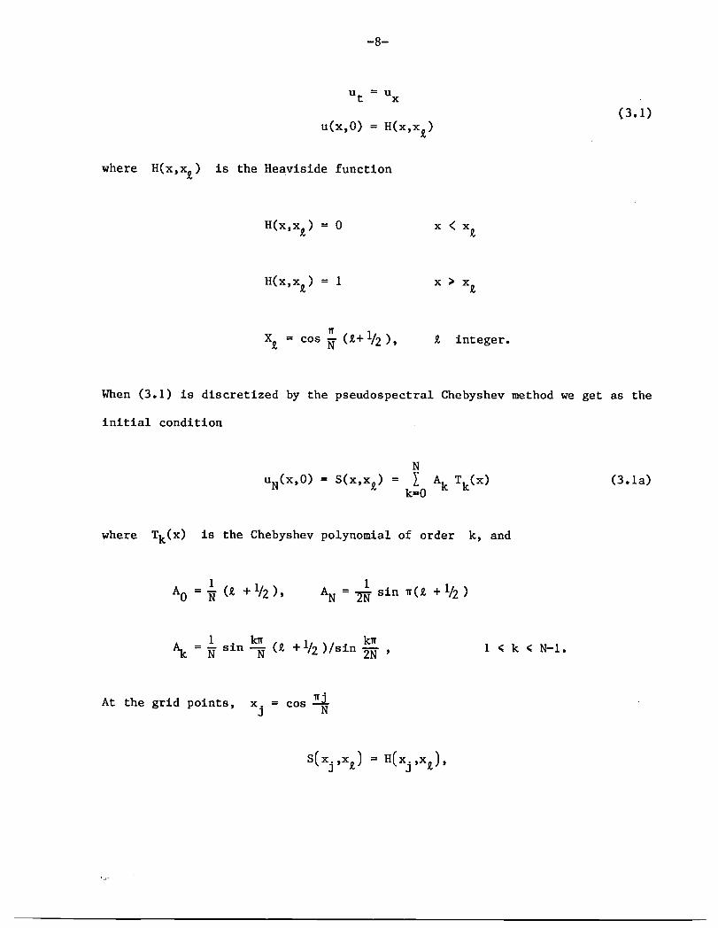
To better understandthe origin of the oscillatorysolution,considerthe

model equation

-8-

Ut ----UX

(3.1)

u(x,0) = H(x,x£)

where H(x,x£) is the Heavlslde function

H(x,x£) = 0 x < x£

H(x,x£) = 1 x ) x £

X£ = cos _ (£+1/2 ), £ integer.

When (3.1) is dlscretlzed by the pseudospectral Chebyshev method we get as the

initial condition

N

UN(X,0) = S(x,x£) = _ Ak Tk(X) (3.1a)k=0

where Tk(X) is the Chebyshev polynomial of order k, and

1 IA0 = _ (£ +1/2), AN = _-_ sln _(£ +1/2)

I _ k_=_ sln (£ +1/2)Isln_-_ , 1 • k • N-I.

At the grid points, x. = cos _j3 N

slxjx_)=Hixjx_)

-9-

Thus, no oscillations occur. However, after the numerical solution is

convected by equation (3.1), it becomes oscillatory. This is because

initially it is oscillatory between the grid points (see Fig. I). Observe

that the oscillations disappear when the discontinuity is exactly in the

middle betweentwo grid points. This demonstratesthe fact that the structure

of the oscillationsprovides informationabout the position and magnitude of

the shock.

3.7 -- 3.7

3.4 3.4 0

3.1 O0 3.1

0

2.8 2.8

• 2.5 • 2.5 0

2.2 2.2

1._ 0 0 0 0 0 0 1.9( 0 00 0

0

l.E 1.6

1.3 1.3

1.0 I I I I I I I I I I 1.0 I I I I I I I f I I-1.0 -.S -.6 -.4 -.2 0 .2 .4 .6 .8 1.0 -1.0 -.8 -.6 -.4 -.2 0 .2 .4 .6 .8 1.0

X axis X axis

3.7

3,4

3.1 0 O0

2.8

• 2.5 --

2.2

I._ 0 0 0 0 0

I._

1.3

z.ol I I I I I I I I I I-1,0 -.8 -.6 -.4 -.2 0 .2 .4 .6 .8 1.0

X axts.

Figure 1

-I0-

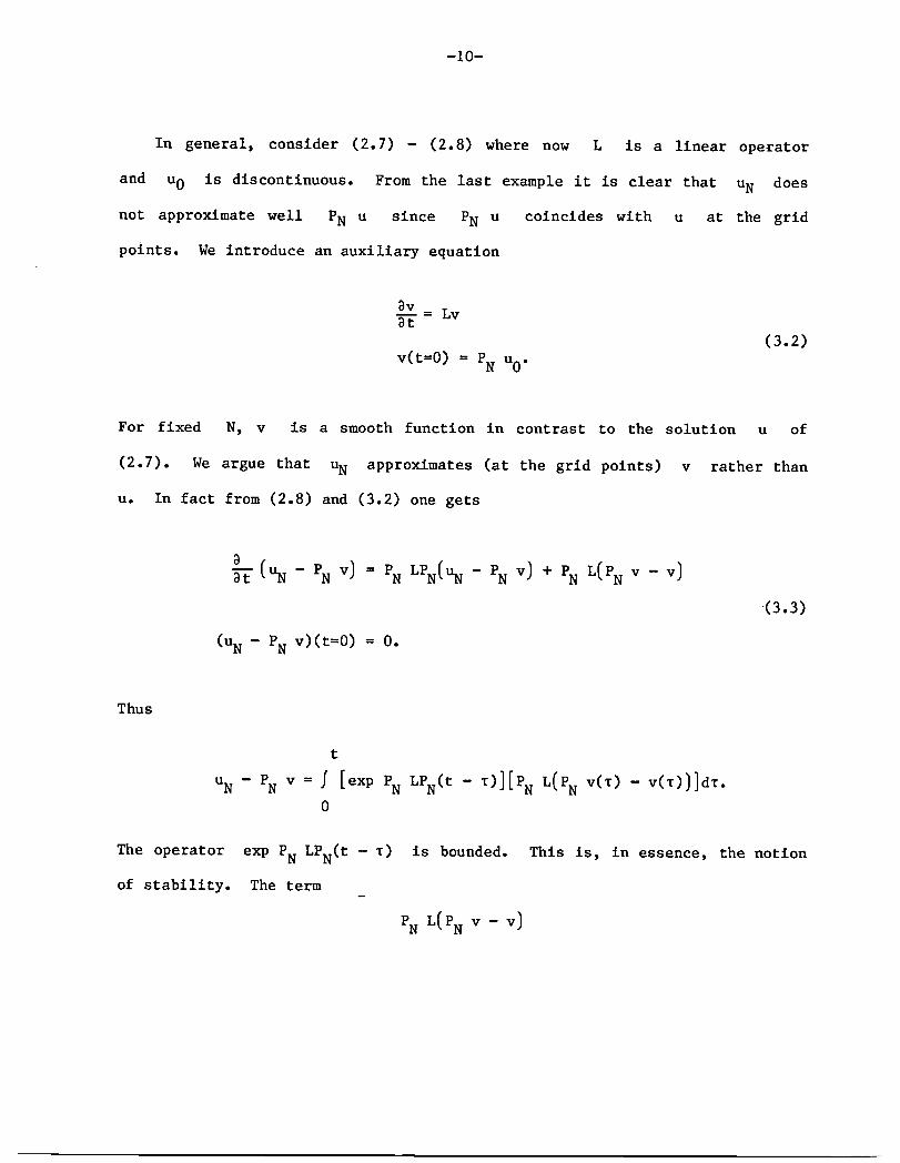
In general, consider (2.7) - (2.8) where now L is a linear operator

and u0 is discontinuous. From the last example it is clear that uN does

not approximate well PN u since PN u coincides with u at the grid

points. We introduce an auxiliary equation

Sv- Lv

St

(3.2)

v(t=0) = PN u0"

For fixed N, v is a smooth function in contrast to the solution u of

(2.7). We argue that uN approximates (at the grid points) v rather than

u. In fact from (2.8) and (3.2) one gets

S

S-_ (UN - PN v) = PN LPN(UN - PN v) + PN L(PN v - v)

(3.3)

(UN - PN v)(t=0) = 0.

Thus

t

UN - PN v = f [exp PN LeN(t - T)][PN L(PN v(_) - v(T))]dT.0

The operator exp PN LPN(t - T) is bounded. This is, in essence, the notion

of stability. The term

PN L(PN v - v)

-II-

is small because v is a smooth function. This shows that uN approximates

PN v, hence at the grid points uN approximates v.

In the last example we have demonstrated the fact the v is, in general,

oscillatory. It is therefore no surprise that uN is oscillatory. It is

also clear that the structure of the oscillations may be used to extract a

better approximation to u.

We will demonstrate now the possibility of extracting information from an

oscillatory solution even in the nonlinear case. The physical problem is the

well-known wedge flow. A plate is inserted in a uniform flow, and an oblique

shock develops. The time dependent Euler equations in two-space dimensions

were discretlzed by the pseudospectral Chebyshev method in space with

a 9×9 grid and a modified Euler scheme was used for the time dlscretlzation

(see [5]). Since we are interested in the steady state only, the accuracy of

the time integration is of no importance. In order to be sure that a steady

state is reached the code was run until all the physical quantities did not

change to II significant figures over a span of I00 time steps. The values of

the density in the steady state at the grid points together with the grid

points themselves are given in Fig. 2.

p Y

1.862 1.851 1.869 1.871 1.837 1.865 1.892 1.885 1.878 I.

1.862 1.870 1.867 1.820 1.870 1.954 1.899 1.803 1.759 .961

1.862 1.854 1.852 1.904 1.877 1.770 1.782 1.864 1.900 .853

1.862 1.871 1.876 1.812 1.838 1.969 1.975 1.884 1.841 .691

1.862 1.848 1.842 1.935 1.899 1.703 1.710 1.890 1.984 .5

1.862 1.883 1.894 1.729 1.832 2.429 2.994 3.255 3.316 .308

1.862 1.808 1.810 2.387 3.133 3.375 3.224 3.054 3.002 .146

1.862 2.115 2.868 3.288 3.176 2.965 3.006 3.136 3.187 .038

1.862 3.083 3.046 2.975 3.087 3.108 3.024 3.013 3.016 0

X 0 .038 .146 .308 .5 .691 .853 .961 I.

Figure2

-12-

Note that at the stations: x0 = I; xI = .9619; x2 = .85355, the jump takes

place between the grid points y = .3086 and y = .5, whereas the

corresponding correct shock location is y = .434 for x0, y = .417 for x1

and y = .370 for x2. Note also that the oscillatory behavior of the density

is very similar to the behavior of PN v, the solution of (3.2) at the grid

points (see Fig. i).

We therefore fit a step-function of the form dI + d2 S(y,y£) where

S(y,y£) is defined in (3.1a) to the numerical results p(y) in Fig. 2, at

any station xj, regarding dl, d2 and £ as unknowns. This yields three

equations

dl f0 + d2 fl = S1

dl fl + d2 f2 = S2 (3.4)

dl f4 + d2 f3 = S3

whe re

N N= 1 = _2 1

fo = N; fl I S(yj,y£) _. ; f2 _ S(yj,y£j _. ;j--0 j j--0 j

N N _S 1

f3 = _" SIyj Y£) _ 1' _£- SIyj'Y£ ) _. ; f4 = "_ (Yj'Y£) ;j=o j j o

N

S1 = _ p(yj) I N Ij 0 "_j ; $2 = I p(yj)S(yj,y£) _. ;j=O j

-13-

$3 p(yj) BS= _-_-(yj,y_)•

Equation (3.4) yields the following nonlinear equation for the shock location

Y%

f0 fl S1

fl f2 S2 = 0 (3.5)

f4 f3 S3

Surprisingly, from (3.5) we recover the correct location of the shock at each

x-station within the fourth significant digit. In this sense the information

is indeed hidden in the form of oscillations.

It should be noted that in (3.4) we do not use the point values of

p(y) but rather the quantities Sl, $2, S3 which are equivalent to the

integral of p(y) against I, S(y,y_) and -_ S(y,y%). If p(y) approxi-

mates well the first N modes of the solution Pext(Y), then

1

f (oCY) - Oext(Y)) _(Y) = 0

-I _1 - y2

_S

where _(y) is either I or S(y,y_) or -_ (y,y%). This may be the reason

for the highly accurate values of the location of the shock obtained by (3.4).

Finally, we would like to describe another way of recovering correct point

values from an oscillatory approximation. For simpiicity we consider the

spectral Legendre method although this idea has been generalized to other

-14-

spectral methods. Our approach is motivated by the work of Mock and Lax (see

[io])•

Suppose that f(x) is a C_ function at Ixl < 1 except for one point

of discontinuity. Suppose also that f(x) has the following expansion in

terms of the Legendre polynomials

oo

f(x) = _. ak Pk(X)k;O

and that

N

iN(x) = _ ak ek(x)•k=0

Even for large N, iN(x) is an oscillatory function• Let y be a point suchoo

that f(x) is C in the interval y-€ < x < y+€. Let

• p1 .q

(I - _2) _ (2k+l)Pk(0)Pk(_) I_I < 1 _ =x-y

k=O €

,(x)=

0 I I>

It is clear that

1 1 1

J fN(x)¢(x)dx --J f(x)*(x)dx + J (iN - f)¢dx.-1 -1 -1

The function _(x) has the expansion

GO

*(x) = _ bk Pk(X)k=O

-15-

and since _(x) has q-I continuous derivative the function _N(X)

N

9N(X) = _ _ Pk(x)k--0

approximates 9 with high accuracy. Moreover, since 9N(X) is a polynomial

of degree N

1 1

f IfN - f)_dx = f IfN - f)[_ - _N)dX ( flf- fNll It_- _N g-I -I

u,(q-l)n

Nq-1

The last estimate can be found in [I].

It is therefore clear that

fN @ dx = I f@ dx + E1

where E1 is small. Moreover,

1 1 P

f(x)_(x)dx = _ f(y+_)(l-_2) q _ (2k+l)ek(0)Pk(_)d_.-i -I k=0

Let

g(_) = f(y + E_)(I- _2)n .

g(_) is a C_ function for I_I < 1 and therefore has a rapidly converging

expansion of the form

-16-

g(_) = _ % Pk (_)"k=O

Therefore

I P p

J g(_) _ (2k+l)ek(0)Pk(_)d_ = _ ck ek (0)

-I k=0 k=0

= g(0) - _ ck = f(y) + E2.k=p+l

This shows that

fN _ dx

approximates f(y) to a high order of accuracy. This filter had been

successfully used by Gottlleb and Gruberger for several problems.

In conclusion we have demonstrated that numerical solutions obtained by

spectral methods contain information about the correct solution that may be

extracted to yield a high order approximation in the regular sense.

-17-

References

[I] Canuto, C. and Quarteroni, A., "Approximation results for orthogonal

polynomials in Sobolev spaces," Math. Comput., 38, 1982, pp. 67-86.

[2] Cornille, D., '_ pseudospectral scheme for the numerical calculation of

shocks," J. Comput. Phys., 47, 1982, pp. 146-159.

[3] Gottlieb, D,, Hussaini, M. Y., and Orszag, S. A., Theory and

Applications of Spectral Methods, Proc. of the Symposium of Spectral

Methods for Partial Differential Equations, SLAM, 1984, pp. 1-55.

[4] Gottlieb, D., Lustman, L. and Orszag, S. A., "Spectral calculations of

one-dimenslonal inviscid compressible flow," SlAM J. Sci. Statis.

Comput., 2, 1981, pp. 296-310.

[5] Gottlleb, D., Lustman, L. and Streett, C., "Spectral methods for two-

dimensional flows," Proc. of the Symposium on Spectral Methods for

Partial Differential Equations, SLAM, 1984, pp. 79-96.

[6] Gottlleb, D. and Orszag, S. A., Numerical Analysis of Spectral

Methods: Theory and Applications CBMS Regional ConferenceSeries in

AppliedMathematics,26, SIAM, 1977.

[7] Gresho,P. and Lee, R. L., "Don't surpressthe wiggles, they'retelling

you something,"Comput.& Fluids, 1981, pp. 223-254.

-18-

[8] Hussalni, M. Y., Koprlva, D. A., Salas, M. D., and Zang, T. A.,

"Spectral methods for Euler equations," AIAA-83-1942-CP, Proc. of the

6th AIAA Computational Fluid Dynamics Conference, Danvers, MA, July 13-

15, 1983.

[9] Hussainl, M. Y., Salas, M. D., and Zang, T. A., "Spectral methods for

invlscld, compressible flows," in Advances in Computational Transonlcs,

W. G. Habshl, ed., Pineridge Press, Swansea, UK, 1983.

[I0] Lax, P. D., "Accuracy and resolution in the computation of solutions of

linear and nonlinear equations," in Recent Advances in Numerical

Analysis, Proc. Symp., Mathematical Research Center, University of

Wisconsin, Academic Press, 1978, pp. 107-117.

[II] Reddy, K. C., "Pseudospectral approximation in three-dlmenslonal

Navier-Stokes code," AIAA J., Vol. 21, No. 8, 1983, pp. 1208-1210.

[12] Sakell, L., "Solution to the Euler equation of motion, pseudospectral

techniques," Proc. 10th IMACS World Congress System, Simulation and

Scientific Computing, 1982.

[13] Salas, M. D., Zang, T. A. and Hussalni, M. Y., "Shock-fltted Euler

solutions to shock-vortex interactions," Proc. of the 8th International

Conference on Numerical Methods in Fluid Dynamics, Lecture Notes in

Physics 170, (E. Krause, ed.), Sprlnger-Verlag, 1982, pp. 461-467.

-19-

[14] Streett, C. L., "A spectral method for the solution of transonic

potential flow about an arbitrary airfoil," AIAA-83-1949-CP, Proc. of

the 6th AIAA Computational Fluid Dynamics Conference, Danvers, MA, July

13-15, 1983.

[15] Taylor, T. D., Myers, R. B., and Albert, J. H., "Pseudospectral

calculations of shock waves, rarefaction waves and contact surfaces,"

Comput. Fluids, 9, 1981, pp. 469-473.

[16] Zang, T. A. and Hussalnl, M. Y., "Mixed spectral/flnltedifference

approximationsfor slightly viscous flows," Lecture Notes in Physics

141..___,Sprlnger-Verlag,1980, pp. 461-466.

[17] Zang, T. A, Kopriva, D. A. and Hussalnl, M. Y., "Pseudospectral

calculation of shock turbulence interactions," Proc. of the 3rd

InternationalConferenceon NumericalMethods in Laminar and Turbulent

Flow, (C. Taylor, ed.), PinerldgePress, 1983.

I. ReportNo. NASA CR-172395 2. GovernmentAccessionNo. 3. Recipient's'CatalogNo.ICASE Report No. 84-29

4. Title andSubtitle 5. ReportDateJune 1984

SPECTRAL METHODS FOR COMPRESSIBLE FLOW PROBLEMS 6. PerformingOrganizationCode

7. Author(s) 8. Performing Organization Report No.

David Gottlleb 84-2910. Work Unit No.

9. Performing Organization Name and Address

Institute for Computer Applications in Science '11. Contract or Grant No.and Engineering

Mail Stop 132C, NASA Langley Research Center NASI-17070

g=mnPnn VA 9"_665 13. Typeof ReportandPeriodCovered12. Sponsoring Agency NameandAddress Contractor Report

14. Sponsoring Agency CodeNational Aeronautics and Space Administration

Washington, D.C. 20546 505-31-83-0115. Supplementary Notes

Langley Technical Monitor: Robert H. Tolson

Final Report

16. Abstract

In this article we review recent results concerning numerical simulation of

shock waves using spectral methods. We discuss shock fitting techniques as well as

shock capturing techniques with finite difference artificial viscosity. We also

discuss the notion of the information contained in the numerical results obtained byspectral methods and show how this information can be recovered.

"17. Key Words (Sugg_ted by Authoris)) 18. Distribution Statement '

spectral methods, 64 - Numerical Analysiscompressible flow problems,shock waves

Unclassified - Unlimited

19. SecurityOassif.(ofthisreport) 20. SecurityClassif.(of this_ge) 21. No. of Pages 22. DiceUnclassified Unclassified 21 A02

ForsalebytheNationalTechnicalInformationService,Springfield,Virginia22161NASA-Langley,1984