nasa · in both cases, the optimization technique generated functions that modeled the test data...

m

NASATechnicalMemorandum

NASA TM - 108394

(NASA-TM-108394) THE ANALYTICAL

REPRESENTATION OF VISCOELASTIC

MATERIAL PROPERTIES USING

OPTIMIZATION TECHNIQUES (NASA)

23 p

G 3/39

N93-19972

Unclas

0150326

THE ANALYTICAL REPRESENTATION OF

VISCOELASTIC MATERIAL PROPERTIES

USING OPTIMIZATION TECHNIQUES

By S.A. Hill

Structures and Dynamics Laboratory

Science and Engineering Directorate

February 1993

iii!_

/

•, /!

NASANational Aeronautics andSpace Administration

George C. Marshall Space Flight Center

MSFC- Form 3190 (Rev. May 1983)

https://ntrs.nasa.gov/search.jsp?R=19930010783 2018-08-26T23:48:25+00:00Z

REPORT DOCUMENTATION PAGE

i

Form Approved

OMB No. 0704-0188

Pub c report ng burden for this collection of information is estimated to average I hour per response, including the time for reviewing instructions, searching existing data sources,

gathering and maintain ng the data needed, and completing and reviewing the collection of information. Send comments regarding this burden estimate or any other aspect of thiscollection of information, ncluding suggestions for reducing th s burden, to Washington Headquarters Serv ces, Directorate for information Operations and Reports, 1215 Jefferson

Davis Highway, Suite 1204, Arlington, VA 22202-4302, and to the Office of Management and Budget, Paperwork Reduct on Project (0704-0188), Wash ngton, DC 20503.

1. AGENCY USE ONLY (Leave blank) 2. REPORT DATE 3. REPORT TYPE AND DATES COVERED

February 1993 Technical Memorandum

4. TITLE AND SUBTITLE 5. FUNDING NUMBERS

The Analytical Representation of Viscoelastic Material Properties

Using Optimization Techniques

6. AUTHOR(S)

S.A. Hill

7. PERFORMINGORGANIZATIONNAME(S)ANDADDRESS(ES)

George C. Marshall Space Flight Center

Marshall Space Flight Center, Alabama 35812

9. SPONSORING/ MONITORINGAGENCYNAMEtS)AND ADDRESStES)

National Aeronautics and Space Administration

Washington, DC 20546

8. PERFORMING ORGANIZATIONREPORT NUMBER

10. SPONSORING / MONITORINGAGENCY REPORT NUMBER

NASA TM-I08394

11. SUPPLEMENTARY NOTES

Prepared by Structures and Dynamics Laboratory, Science and Engineering Directorate.

12a. DISTRIBUTION / AVAILABILITY STATEMENT

Unclassified -- Unlimited

12b. DISTRIBUTION CODE

13. ABSTRACT (Maximum 200words)

This report presents a technique to model viscoelastic material properties with a function of the form of

the Prony series. Generally, the method employed to determine the function constants requires assuming values

for the exponential constants of the function and then resolving the remaining constants through linear least-

squares techniques. The technique presented here allows all the constants to be analytically determined through

optimization techniques.

This technique is employed in a computer program named PRONY and makes use of commercially

available optimization tool developed by VMA Engineering, Inc. The PRONY program was utilized to compare

the technique against previously determined models for solid rocket motor TP-H1148 propellant and V747-75

Viton fluoroelastomer. In both cases, the optimization technique generated functions that modeled the test data

with at least an order of magnitude better correlation. This technique has demonstrated the capability to use

small or large data sets and to use data sets that have uniformly or nonuniformly spaced data pairs.

The reduction of experimental data to accurate mathematical models is a vital part of most scientific and

engineering research. This technique of regression through optimization can be applied to other mathematical

models that are difficult to fit to experimental data through traditional regression techniques.

14. SUBJECT TERMS

Optimization, Prony Series, Viscoleastic, Stress Relaxation

17. SECURITYCLASSIFICATION18. SECURITYCLASSIFICATION19. SECURITYCLASSIFICATIONOFREPORT OF THISPAGE OF ABSTRACT

Unclassified Unclassified Unclassified

NSN 7540-01-280-5500

15. NUMBER OF PAGES

2416. PRICE CODE

NTIS

20. LIMITATION OF ABSTRACT

Unlimited

Standard Form 298 (Rev. 2-89)

TABLE OF CONTENTS

INTRODUCTION .........................................................................................................................

DESCRIPTION OF THE TECHNIQUE .......................................................................................

COMPUTER IMPLEMENTATION .............................................................................................

NUMERICAL EXAMPLES .........................................................................................................

SRM TP-H1148 Propellant ................................................................................................V747-75 Viton Fluoroelastomer ........................................................................................

CONCLUSIONS ............................................................................................................................

REFERENCES ...............................................................................................................................

APPENDIX A - PRONY Source Code Listing ............................................................................

APPENDIX B - V747-75 Viton Stress Relaxation Data ..............................................................

APPENDIX C - PRONY Program Output Files ..........................................................................

SRM TP-H1148 Propellant ...............................................................................................V747-75 Viton Fluoroelastomer ........................................................................................

Page

1

2

4

5

56

9

11

13

15

16

16

17

%(. *

iii PRBOEDING P,_IG'E BLANK NOT FILM, ED

Figure

1.

2.

3.

4.

5.

LIST OF ILLUSTRATIONS

Title

Relation of constraints to an objective function ..........................................................

Comparison of Prony series functions, Rodriguez versus optimized methods ...........

Comparison of Prony series functions, Rodriguez versus optimized methods ...........

Comparison of Prony series functions, classical versus optimized methods ...............

Comparison of Prony series functions, classical versus optimized methods ...............

Page

3

7

7

10

10

Table

1.

,

3.

4.

LIST OF TABLES

Title

Stress relaxation results of SRM TP-H1148 propellant at-30 °F and

2-percent strain ............................................................................................................

Sensitivity study results for SRM TP-H1148 propellant .............................................

Classically derived Prony coefficients ........................................................................

Sensitivity study results for V747-75 Viton ................................................................

Page

iv

TECHNICAL MEMORANDUM

THE ANALYTICAL REPRESENTATION OF VISCOELASTIC MATERIAL

PROPERTIES USING OPTIMIZATION TECHNIQUES

INTRODUCTION

One of the purposes of performing tests--either static, dynamic, mechanical, or electrical--is to

determine the response of a system to a set of given test inputs. This test information can be reduced to a

function of the system response, the dependent variable, to the test inputs, or the independent variables.

This model can then be used to predict intermediate cases that are uneconomical to test. In the specific

case of modeling the time-dependent properties of viscoelastic materials, it is particularly important that

an accurate characterization of these properties be developed so that additional sources of error are not

introduced into the solutions of problems involving these properties.

A popular method used for formulating an analytical model for these time-dependent properties

is to curve fit the test data to a predefined model, such as the Prony series. The Prony series can bedefined as

f (t) = A +Y-d3ie _'it , (1)

where t is defined as the independent variable, f(t) as the dependent variable, and A, Bi, and _ are func-

tion constants. The difficulty in reducing test data to the Prony series model is that the number of

knowns in the model is exceeded by the number of unknowns. When this is encountered using tradi-

tional methods, usually the only recourse is to assume values for some of the unknowns.

In the case of the Prony series, the values for the exponential constants, _, are assumed to follow

a decade pattern (i.e., Yt = -1, Y2 = -10, _ = -100 .... ). With the ?_ terms defined, the constants A and Bi

can be solved for using least-squares regression techniques. The major drawback to this method is that

the function is only as accurate as the values assumed for _.

Rodriguez 1 presented a method in which the Prony series could be fit to test data using two

Prony terms. This method allowed for the analytical solution of all constant terms. The only drawback to

this method lay in the fact that the small number of Prony terms allowed for in this method may notcharacterize all the subtleties of the test data, thus the need for higher order terms in the function.

The technique presented in this report allows data to be fit to the Prony series without the need

for assuming values for the _ terms. This technique determines the "optimum" Prony series function

based on the input data and on minimizing the difference between the actual and calculated dependent

variable. This report will expand on the method employed to determine the "optimum" function and will

present some numerical examples to demonstrate the robustness, speed, and accuracy of the method.

The computer program that was developed to perform the analysis was written in FORTRAN 77,

and the analyses were performed on a 25-MHz 80386 PC with a math coprocessor installed.

DESCRIPTION OF THE TECHNIQUE

Recently, more and more emphasis has been placed on the design of structures that are light-

weight yet offer high strength of stiffness. In order to achieve the minimum weight designs, optimization

techniques and algorithms have been developed throughout the design community. One of the tools

employed by the Structural Development Branch at Marshall Space Flight Center (MSFC) is the Design

Optimization Tool (DOT) by VMA Engineering, Inc. 2

DOT is a general optimization code written in FORTRAN 77 that will perform either constrained

or unconstrained optimization, given the necessary design variables, constraints, and objective function.

In order to access the optimization routines located within the DOT code, a header program is written

that contains the definition of the initial DOT parameters; the initial value, lower bound, and upper

bound for all design variables; a description of the objective function; a description of the functions

required to constrain the design variables; and a calling statement to the DOT program.

There are three optimization algorithms available with the DOT code for the solution of opti-

mization problems. The first method, the Broydon-Fletcher-Goldfarb-Shanno (BFGS) algorithm, is

employed only in unconstrained optimization problems. The other two available methods, the modified

method of feasible directions (MMFD) and sequential linear programming (SLP), can be employed in

the solution of constrained optimization problems.

The technique developed in this report is an unconstrained optimization method and, therefore,

employs the BFGS algorithm to minimize the objective function. The term "unconstrained optimization"

means that the function being optimized (i.e., the objective function) is not restrained to any design

space. Although this technique employs an unconstrained optimization method, it is not truly uncon-

strained. The design variables (i.e., variables that can be manipulated in order to achieve a minimized ormaximized objective function) are restrained through the use of side constraints which limit the range of

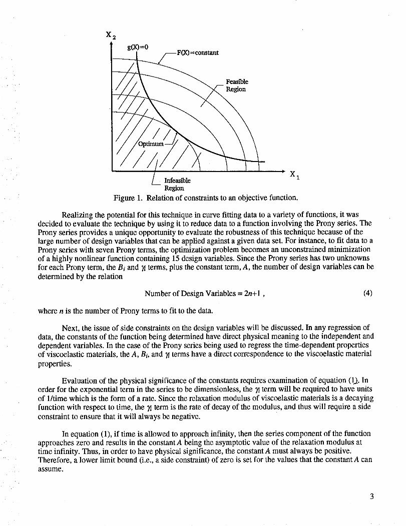
values any one design variable can assume. The relation of constraints and side constraints to the objec-

tive function are depicted in figure 1 (from ref. 2).

In the evaluation of analytical data for an unrelated problem, it was found that the correlation of a

function, derived through linear least-squares techniques, to a particular set of data could be improved

through slight manipulation of the constant terms of the function. This led to the implementation of the

DOT code to solve for the constants of a given function through the minimization of the sum of the

residuals squared. The sum of the residuals squared gives a direct measurement of the accuracy of thecurve fit and is defined as

Sr = _.(f(xi)_Yi) 2 , (2)

where f(xi) is defined as the value of the derived function at a given value of the independent variable,

and Yi is the value of the dependent variable at the same independent variable value. Basically':the sum

of the residuals squared reveals how close the function comes to passing through all the data points. Thisresult is then used to calculate the correlation coefficient of the function. The correlation coefficient is

also used to determine the accuracy of the curve fit, but reveals the percentage of error in the fit that is

not explained by the function. The correlation coefficient is given by

_/St-Str = St ' (3)

where St is defined as the variance of the data about its mean.

2

X 2

gO0--O nstant

_-- Feasible

L_. InfeasibleRegion

Figure 1.

X1

Relation of constraints to an objective function.

Realizing the potential for this technique in curve fitting data to a variety of functions, it was

decided to evaluate the technique by using it to reduce data to a function involving the Prony series. TheProny series provides a unique opportunity to evaluate the robustness of this technique because of the

large number of design variables that can be applied against a given data set. For instance, to fit data to a

Prony series with seven Prony terms, the optimization problem becomes an unconstrained minimization

of a highly nonlinear function containing 15 design variables. Since the Prony series has two unknowns

for each Prony term, the Bi and 7/terms, plus the constant term, A, the number of design variables can be

determined by the relation

Number of Design Variables = 2n+l, (4)

where n is the number of Prony terms to fit to the data.

Next, the issue of side constraints on the design variables will be discussed. In any regression of

data, the constants of the function being determined have direct physical meaning to the independent and

dependent variables. In the case of the Prony series being used to regress the time-dependent properties

of viscoelastic materials, the A, Bi, and 7/terms have a direct correspondence to the viscoelastic material

properties.

Evaluation of the physical significance of the constants requires examination of equation (U. In

order for the exponential term in the series to be dimensionless, the 7_term will be required to have units

of 1/time which is the form of a rate. Since the relaxation modulus of viscoelastic materials is a decaying

function with respect to time, the _ term is the rate of decay of the modulus, and thus will require a side

constraint to ensure that it will always be negative.

In equation (1), if time is allowed to approach infinity, then the series component of the function

approaches zero and results in the constant A being the asymptotic value of the relaxation modulus at

time infinity. Thus, in order to have physical significance, the constant A must always be positive.Therefore, a lower limit bound (i.e., a side constrain0 of zero is set for the values that the constant A can

assume.

3

Now, if time is allowedto approachzero,then all the exponential terms in the series component

will approach one. Thus, the relaxation modulus at time zero is the summation of the constant A and theBi terms. Therefore, the Bi terms are also directly related to the relaxation modulus and, thus, require a

side constraint on the lower bound to maintain positive values for all the Bi terms.

COMPUTER IMPLEMENTATION

Appendix A contains the FORTRAN 77 source code for the program PRONY which reduces

data to the Prony series form based on the implementation of the DOT optimization subroutines.

The program first initializes the variables necessary for the DOT subroutines to perform the

optimization. The program then prompts the user for a data input filename, an output filename, and the

number of Prony terms to be used.

Next, the side constraints for each of the design variables are set to zero and either a large posi-

tive or negative number, dependent upon whether the variable is allowed only positive or negative

values, respectively. Then a call is made to a subroutine where the input file is opened, the xi and Yi data

pairs are read, and the mean value and variance of the dependent variable are calculated. Next, the loop

is entered that controls the iterative process of performing the optimization task. Upon meeting the con-

vergence criteria, the loop is exited, and the subroutine EVAL is evaluated to ensure that the objectivefunction and the sum of the residuals squared are evaluated with the final values of the design ,_ariables.

Finally, the output subroutine is called to send the results of the optimization to disk file.

Now that the subject of design variables, constraints, side constraints, and the objective function

have been discussed, it is time to briefly mention some of the other parameters that are required to per-

form the optimization task through DOT. The first item to discuss is the convergence criteria. DOT uses

two user-definable variables to control the convergence, the first being an absolute criteria and thesecond a relative criteria.

If the initial value of the objective function is changed by less than the value for the absolute cri-

teria during the optimization process, then the optimization task is assumed to have converged and will

terminate. 2 The relative criteria will stop optimization when the relative change between the objective

function in any two successive iterations is less than or equal to this variable. Since the objective func-

tion generally assumes a large value on the initial calculation, because the initial values of the design

variables are usually far from the optimum values, the Prony ser;_- program relies on the relative criteria

to control convergence. .-

The other remaining item to discuss concerning the implementation of the DOT.code in the

reduction of data to a Prony series function is the variable that controls the number of consecutive itera-

tions that must satisfy the convergence criteria before optimization is terminated. By default, the DOT

code sets this variable equal to two, since it is common to make little progress on one iteration, only to

make significant progress on the next. It is suggested that if consistent progress is made on optimizing

the objective function and if computer time is inexpensive, then this value can be raised. The PRONY

program automatically overrides the default value and sets the variable equal to three, based upon test

runs that showed additional improvement with the increased number of iterations.

NUMERICAL EXAMPLES

_ii/ •

Solid Rocket Motor TP-Hl148 Propellant

Modeling the relaxation modulus of solid rocket motor (SRM) TP-H1148 propellant wasselected as the first case since it was used as a numerical example by Rodriguez, 1 thus giving a direct

comparison between the two methods. The data used by Rodriguez were obtained from a stress relax-

ation test of SRM TP-H1148 propellant that was tested at -30 °F and 2-percent strain. 3 The time varyingrelaxation moduli are listed in table 1.

Table 1. Stress relaxation results of SRMTP-H1148 propellant

at-30 °F and 2-percent strain.

Time (min) Er (lb/in 2)

1.66×10 -3

6.61x10-3

1.66×10 -2

4.17x10 -2

8.32x10 -2

1.26×10 -2

1.66×10 -1

1.66×100

1.66x101

21,114

12,913

10,99210,114

8,399

7,566

7,0883,568

1,981

Rodriguez plotted the data points and fit a third-order B-spline curve to the data using an

Intergraph computer-aided design (CAD) package called IGDS. Nineteen evenly spaced data points

were then selected from the portion of the B-spline curve between 0.002 and 0.020 min. (Note: One of

the requirements of the technique developed by Prony and used by Rodriguez is that the data points be

spaced at equal time increments.) The constants A, B1, _tl, B2, and _ were determined to be 10,973.3,

23,397.2, -380.8698, -79,056.7, and-1,971.8239, respectively.

Comparing this curve-fitted Prony function to the actual test data through equations (2) and (3)

yields a sum of residuals squared of 1.71 x 108 and a correlation coefficient of 0.566609. On initial

inspection, this method does not appear to generate a precise fit of the data points, but if the function is

compared to the data points that basically fall within the aforementioned 0.002- and 0.020-min timeinterval, then a sum of residuals squared of 1.18xl 06 and a more impressive correlation coefficient of

0.992128 are yielded.

As a comparison of the Rodriguez method and the optimization method, a series of runs was

made using the Prony program and the TP-H1148 test data. These runs were made in an effort to deter-

mine the sensitivity of the method to the initial starting point of the design variables and to the number

of Prony terms utilized in the analysis. The output file listing generated by the Prony program for eachof the cases listed in table 2 is contained within appendix C. Each file contains the date and time of the

run, the input parameters, the sum of the residuals squared, the values for the A, B i, and ?i terms, the

correlation coefficient, and the central processing unit (CPU) time required for the analysis.

Table2. Sensitivitystudyresultsfor SRMTP-H1148propellant.

i

Prony Terms

2

Sums of Residuals

Squared

CorrelationCoefficient Run Time (s)

1,427,300.1 0.99716 1.4

3 82,166.3 0.99984 3.0

4 82,201.7 0.99984 3.5

5 83,250.0 0.99983 6.6

Referring to table 2, it can be seen that the first case of two Prony terms yielded a sum of residu-

als squared that was 99.17 percent lower than that yielded by the Rodriguez method. The remainingthree cases of three, four, and five Prony terms appear to have reached a lower bound on the sum of

residuals squared that is approximately 94.24 percent lower than the case with two Prony terms. In all

four cases analyzed, the CPU time required to run the analyses was insignificant due to the small number

of data points available for the curve fit.

Figures 2 and 3 graphically depict the relationship between the data points, the second-order

Prony function derived from the Rodriguez method, and the second- and fourth-order Prony functions

derived through the optimization technique, respectively. The figures show that the Rodriguez Prony

function accurately models the propellant behavior over the time interval in which it was developed

(0.002 to 0.020 min). It does not accurately model the late time behavior of the propellant. The second-and fourth-order optimized Prony functions, on the other hand, appear to accurately model the subtle

fluctuations in the test data over the full-time interval. The apparent faceted nature of the curves in

figures 2 and 3 is a direct result of the respective functions being plotted only at the test data points.

V747-75 Viton Fluoroelastomer

The second example also involves the time-dependent relaxation modulus of a viscoelasticmaterial. This time the data were obtained from a stress relaxation test of the V747-75 Viton fluoro-

elastomer. The stress relaxation test was conducted by the Polymers and Composites Branch at MSFC

on an RDS-7700 dynamic spectrometer at 1-percent strain 4 and was shared with the author for thepurpose of evaluating the subject technique. The data generated from this test and then used by the

PRONY program are listed in appendix B.

The data were originally fit to a 14-term Prony function that was developed in the classical

method of assuming values for the _ terms, linearizing the resulting function, and then solvingfor the Aand B i terms through least-squares techniques. The values for the constants A, Bi, and _ terms

determined from this technique are given in table 3.

The resultant Prony function generated from applying these classically derived coefficients

yields a sum of residuals squared of 9.20×106 and a correlation coefficient of 0.968443 when compared

to the test data. This high correlation coefficient shows that the regressed function compares very wellwith the test data.

6

25000-

20000

v15000

0

2

o 10000'

0

W

50O0

Figure 2.

ii i i i i iii I i 1 i i i i ii I i i i i i i ii I i i i i i iii I

10 "= 10 -t 10Time (sec) - - Roa_q.,=- 2 _,rrr4

eeeso Test IRIIO -- Ol_tlmlzed 2 7orn_

Comparison of Prony series functions, Rodriguez versus optimized methods.

25000 ]

"_'20000 1 _ _

i' o°oi111- 50011 ........ , ........ , ....... i , ,

10 -3 10 -' 10Time(sec) - - R_q.,,- _,..,

ee_*• Tnt Doto -- Optlmtzed 24 1"•an=

Figure 3. Comparison of Prony series functions, Rodriguez versus optimized methods.

7

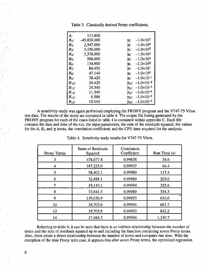
Table 3. Classically derived Prony coefficients.

A: 111.800

BI: -45,830.000 YI: -1.0x107

B2: 2,547.000 _2: -1.0x106

B3: 3,156.000 _: -1.0xl05

B4" 1,378.000 ?'4: -1.0x104

B5: 506.000 ?'5: -1.0×103

B6" 134.900 ?'6: -1.0 x102

BT: 86.450 O: -1.0xl01

Bs: 47.140 _8: -1.0xl0 °

B9: 38.420 _: -1.0xl0 -1

Blo: 26.420 ?'1o: -1.0x10 -2

Bll: 24.340 ?'11:-1.0xl0 -3

B12: 11.540 ?'12:-1.0×10 -4

B13: 6.586 ?'13:-1.0x10-5

B 14: 15.010 ?'14: -1.0x 10-6

A sensitivity study was again performed employing the PRONY program and the V747-75 Viton

test data. The results of the study are contained in table 4. The output file listing generated by the

PRONY program for each of the cases listed in table 4 is contained within appendix C. Each file

contains the date and time of the run, the input parameters, the sum of the residuals squared, the valuesfor the A, Bi, and 3 terms, the correlation coefficient, and the CPU time required for the analysis.

Table 4. Sensitivity study results for V747-75 Viton.

Sums of Residuals Correlation

PronyTerms Squared Coefficient Run Time(s)

3 478,677.4 0.99838 34.6

4 187,225.0 0.99937 64.4

5 58,402.1 0.99980 117.4

6 32,888.1 0.99989 205..0

7 19,110.1 0.99994 355.6

8 33,641.3 0.99989 334.3P

9 139,630.9 0.99953 610,6

10 19,703.0 0.99994 661.7

12 19,705.8 0.99993 842.2

14 17,484.3 0.99994 1,330.7

Referring to table 4, it can be seen that there is an indirect relationship between the number of

terms and the sum of residuals squared up to and including the function containing seven Prony terms.

Also, there exists a direct relationship between the number of terms and computer run time. With the

exception of the nine Prony term case, it appears that after seven Prony terms, the optimized regression

hasbasicallyreachedits lower limit for thesumof residualssquared.Thesmalldecreasesin thesumoftheresidualssquaredarenot worth theadditionalrun time of theprogram,but theCPUtime onaPCisvirtually free,and,if theuserhasthepatience,theadditionalaccuracyaffordedwith the 14thorderPronyfunction maybeworth thewait. An additionalconsiderationthatwill affecttheselectionof theorderof curveto useis the intendeduseof thefunction.If thefunctionis to beusedin "simple" handcalculationsor shortcomputerprograms,thenthehigher-ordercurvemaybeselected.However,if thefunctionis to beusedin nonlinearstressanalysisapplications(i.e.,applicationsin which asignificantnumberof calculationswill beperformedwith thefunction),oneof the lower-orderfunctionsshouldbeselectedto reduceanalysistimes.

Figures4 and5 graphicallydepicttherelationshipbetweenthedatapoints,theclassicallyderived14thorderPronyfunction,andthe7thand14thorderPronyfunctionsderivedthroughtheoptimizationtechnique,respectively.Thesetwo figuresrevealtheexcellentcorrelationbetweenthedataandtheoptimallydeterminedPronyfunctions.Thiscorrelationis mostpronouncedattheearlier timeintervalssincethehigherrelaxationmoduli atthesetimesartificially weight theoptimizationmethodandresultin a betterfit. At the latertimes,therelaxationmoduli aresmaller,and,thus,differencesbetweenthefunctionandthedataat thesetimeintervalscontributelessto thesumof theresidualssquared(equation(2)). Therefore,attheselater times,thefunctionhasmoreof atendencyto "wander"from theactualdatathanat theearliertimes.

CONCLUSIONS

Application of optimization techniques to the task of reducing experimental data to an equivalent

function of the form of the Prony series has been demonstrated. This technique generates functions that

show excellent correlation to their original experimental data, as shown in the previous two numerical

examples. It appears from the numerical examples that the technique is fairly robust, since it reduced

data sets as small as 18 data pairs and as large as 99 data pairs. Also, the technique displayed the

capability to reduce data sets containing data pairs spaced at varying time increments.

It has been previously noted that this regression through optimization technique can generate

functions that are artificially weighted to fit larger ordinate values more accurately than smaller ones.

This artificial weighting was most apparent in the V747-75 Viton numerical example in which the

function more closely approximated the experimental relaxation modulus at the early time intervals,where the modulus varied between 6,000 and 1,000 lb/in 2, than at later times, where the modulus was

less than 1,000 lb/in 2. A few techniques were employed to attempt to minimize this residual weighting

effect. Both normalization of the sum of residuals squared by the mean and changing the objective

function so that the sum of the residuals would be minimized were attempted and generated poorer

correlation of the resulting function to the experimental data. One method yet to be attempted is to

decrease the frequency at which the large ordinate data pairs appear in the data set. Bower 5 states that

this technique shows promise in a similar technique.

As was stated previously, the reduction of experimental data to accurate mathematical models is

a vital part of most scientific and engineering research. This technique of regression through optimiza-

tion can be applied to other mathematical models that are difficult to fit to experimental data through

traditional regression techniques. The author has also employed this technique to fit an n independent

variable power function to experimental data with a resultant function that more accurately predicts

values for the dependent variable than a function generated through traditional regression techniques. In

fact, the FORTRAN code for the program PRONY that is listed in appendix A would require minimal

changes to determine coefficients for a wide range of mathematical models.

6000.

5ooo,

_ooo ,\

__2000'

:i \

I000 1 -, : :-::

illlll l l lllllll l I I Illlll_ I Illllm I l l Illlll| l I lllll| I I lllll| I llmlll I m Illllll I Illllll[ I lllllll I l lllllll| lI10 .-4 10-= 1 10 z 10 `+ 10 °

Time(sec) - -c_,,_ - ,,T,_oeooo Telil 0¢1o -- OpUmized - 7 Tqrrrm

Figure 4. Comparison of Prony series functions, classical versus optimized methods.

6000

5000

._-4000

3000.0

U

2000

1000

Figure 5. Comparison of Prony series functions, classical versus optimized methods.

10

REFERENCES

1. Rodriguez, P.I.: "On the Analytical Determination of Relaxation Modulus of Viscoelastic Materials

by Prony's Interpolation Method." NASA TM-86579, December 1986.

2. Vanderplaats, G.N.: "DOT Users Manual." Version 2.04, Vanderplaats, Miura, and Associates, Inc.,1989. -

3. Harvey, A.R.: "Strain Evaluation Cylinder Study and Propellant Characterization for TP-H1148

SRM Propellant." TWR-14153, January 1984.

4. F.E. Ledbetter HI, private communication.

5. Dr. M.V. Bower, private communication.

11

APPENDIX A

PRONY Source Code Listing

C ****** Prony Curve Fit ******

C * Written By: Scott A. Hill *C *****************************

PARAMETER (converge=0.00001}PARAMETER (itermax = 999)

PARAMETER (itercon - 3)

DOUBLE PRECISION r2, sumt,obJ

CHARACTER*f2 In,Out

DIMENSION x(41),xl(41),xu(41)

DIMENSION a(2000),y(2000)DIMENSION wk(2200)

DIMENSION rprm(20)

DIMENSION g(1)DIMENSION iwk(120)

DIMENSION iprm(20)

C INITIALIZE REAL AND INTEGER WORKSPACE FORDOT

DO 10 i=1,20

rprm (i) =0.0

iprm (i) -010 CONTINUE

rprm(3) - converge

rprm(4) - converge

iprm(3) - Itermaxiprm(4) - itercon

C DEFINE # OF DESIGN VARIABLES, # OF CONSTRAINTS, AMT OF

C DOT OUTPUT & WHETHER PROBLEM IS MINIMIZATION OR

C MAXIMIZATION.

nrwk=2200

nrlwk=120

ncon=0

iprlnt=0mlnmax=-i

method=l

C. DEFINE INITIAL VALUES AND UPPER/LOWER BOUNDS FOR DESIGN

C VARIABLES

WRITE (*,15)

READ (*,' (A)') In

15 FORMAT (' Input File: '\)

WRITE (*,16)READ (*,'(A)') Out

16 FORMAT (' Output File: '\)

WRITE (*,17)

READ (*,*) ndv

17 FORMAT(' # of Prony Terms:'\)

ndv - 2*ndv + 1

x(1) - 150.0

xl(1) - 0.0

xu(1) - 1.0E+25

DO 20 i-2,ndv, 2

x(i) = 500.0

x(i+l) = -3000.020 CONTINUE

DO 25 i - 2,ndvxl(i) - 0.0

xu(i) = 1.0E+2525 CONTINUE

C READ IN DATA & PERFORM STATISTICAL FUNCTIONS

CALL InData (a,y, fen, sumt)

C READY TO OPTIMIZE

info-0

DO WHILE (.TRUE.}

CALL DOT (in fo, met hod, iprint, iprint, ndv,

ncon, x, xl, xu, obJ, minmax, g, rprm,iprm, wk, nrwk, iwk, nriwk)

CALL EVAL (obJ, x, y, a, sumt, fen, r2, ndv)

IF (info.EQ.0} EXIT

END DO

C OPTIMIZATION COMPLETE -- OUTPUT RESULTS

CALL EVAL (obJ, x, y, a, sumt, fen, r2, ndv)

CALL OutPut (obJ,x, ndv, r2, iprm (19), Type)

END

****************************************************

C SUBROUTINE TO EVALUATE FUNCTION AND CONSTRAINTS

****************************************************

SUBROUTINE EVAL (obJ, x, y, a, sumt, len, r2, n,dv)

REAL*8 sumt, r2,Value

REAL*8 obJ, fx

DIMENSION x (*)

DIMENSION y (*), a (*)

obJ - 0.0

DO 100 I = 1,1en

fx = Value (x,a (i),ndv)

obJ - obJ + (y(i) - fx)*(y(i) - fx)100 CONTINUE

r2 - (sumt - obJ)/sumt

RETURN

END

**********************************************

C FUNCTION TO CALCULATE VALUE OF PRONY SERIES

************************************************

REAL*8 FUNCTION Value (array, x, n)

REAL*8 dv

DIMENSION array (*) "

Value - array(1)

DO 200 i - 2,n-I,2

dv - array (i+l)*x

Value = Value + array (i)*DEXP (dv)200 CONTINUE

END

3O

DO 30 i-3, ndv, 2

xl(i) - -I.0E+25xu(i) - 0.0

CONTINUE

,'k_'_k;_k_,_J._.'.. , _,,..,P_E'_k'_D'!NG P,ak_-E B[.,A_.]K NOT FILIWED 13

C****************************************

C SUBROUTINE TO GET DATA FROM INPUT FILE*****************************************

SUBROUTINE InData(a,y, len, sumt)

REAL*8 mean, sumtCHARACTER*f2 In

DIMENSION a (*5 ,Y (*5

Io = 0

fen - 0

sum = 0.0sumt - 0.0

OPEN(I,FILE-In, STATUS-'OLD'5

DO 500 i - I, 1000

READ(1,*,END=5105 a(1),y(1)500 CONTINUE

510 CLOSE(1,STATUS='KEEP')

fen - i - 1

DO 520 i = 1,1en

sum = sum + y(i)520 CONTINUE

mean = sum/fen

DO 530 i - 1,1en

sumt - sumt + (y(i) - mean) * (y (i) - mean5530 CONTINUE

RETURNEND

613

620

630

640

FORMAT(/5X,'Prony Equation Form: y = A + ',AI,• 'Bxe^(',Al,'t) ' )

FORMAT(//5X,'Sum of the Residuals Squared: ',• FI4.4//',F14.4//12X,'A: ',F14.6)

FORMAT(10X,'B',I2,': ',FI4.6,15X,AI,I2,': ',F14.65

FORMAT(/5X,'Correlatlon Coefficient: ',F9.7//

5X,'# of Iterations:',I3)

CLOSE (2,STATUS='KEEP')

RETURN

END

*****************************************

C SUBROUTINE TO SEND DATA TO OUTPUT FILE*****************************************

SUBROUTINE OutPut(obJ,x, ndv, r2,iter)

REAL*8 obJ,r2CHARACTER*f2 In,Out

DIMENSION x(*)

OPEN (2,FILE-Out,STATUS='UNKNOWN'5

k - 0

WRITE (2,610} CHAR(228),CHAR(231)

WRITE (2,611) In

WRITE (2,612) 150.0,500.0,CHAR(231),-1000.0,CHAR(231),0.0,0.000001

WRITE(2,6205 obJ,x(1)

DO 600 i - 2, ndv-l,2k=k+l

WRITE (2,630) k,x(i),CHAR(231),k,x(i+15600 CONTINUE

WRITE(2,640) DSQRT(r2),Iter

610 FORMAT(/5X,'Prony Equation Form: y - A + ',

• AI,'Be^(',AI,'t5 ,}

611 FORMAT(/5X,'Input File: ',AS

612 FORMAT(//5X,'Initial Value for A: ',FI2.4/5X,

'Initial Value for B:',Fl2.4/SX,'Initial Value',

' for ',A,': ',Fl2.4/5X,'Upper Limit for ',A,': ',F12.4 //5X,'Convergence Criteria: '

,F12.10)

14

APPENDIX B

V747-75 Viton Stress Relaxation Data

Time (min)3.6700E-06

4.8090E-06

6.3000E-06

8.2550E-06

1.0820E-05

1.4170E-05

1.8570E-05

2.4330E-05

3.1880E-05

4.1770E-05

5.4720E-05

7.1700E-05

9.3950E-05

1.2310E-04

1.6130E-04

2.1130E-04

2.7690E-04

3.6280E-04

4.7530E-04

6.2280E-04

8.1600E-04

1.0690E-03

1.4010E-03

1.8350E-03

2.4050E-03

3.1510E-03

4.1290E-03

5.4090E-03

7.0880E-03

9.2870E-03

1.2170E-02

1.5940E-02

2.0890E-02

2.7370E-02

3.5860E-02

4.6990E-02

6.1560E-02

8.0660E-02

1.0570E-01

1.3850E-01

1.8140E-01

2.3770E-01

3.1150E-01

4.0810E-01

5.3470E-01

7.0060E-01

9.1800E-01

1.2030E+00

1.5760E+00

E__ (Dsi)5.6500E+03

5.3240E+03

4.8970E+03

4.4720E+03

4.1130E+03

3.7880E+03

3.4710E+03

3.1760E+03

2.8910E+03

2.6240E+03

2.3760E+03

2.1530E+03

1.9470E+03

1.7710E+03

1.6130E+03

1.4810E+03

1.3530E+03

1.1850E+03

1.0590E+03

9.4020E+02

8.5680E+02

7.8990E+02

7.3480E+02

6.8780E+02

6.4450E+02

6.0100E+02

5.5750E+02

5.2570E+02

4.9600E+02

4.6860E+02

4.4330E+02

4.2210E+02

4.0390E+02

3.8690E+02

3.7290E+02

3.6500E+02

3.5740E+02

3.4750E+02

3.3350E+02

3.2100E+02

3.1100E+02

3.0070E+02

2.9330E+02

2.8600E+02

2.7680E+02

2.7220E+02

2.6610E+02

2.5990E+02

2.5340E+02

Time (rain}2.0650E+00

2.7050E+00

3.5450E+00

4.6450E+00

6.0850E+00

7.9730E+00

1.0450E+01

1.3690E+01

1.7930E+01

2.3500E+01

3.0790E+01

4.0340E+01

5.2860E+01

6.9260E+01

9.0740E+01

1.1890E+02

1.5580E+02

2.0410E+02

2.6740E+02

3.5040E+02

4.5910E+02

6.0150E+02

7.8820E+02

1.0330E+03

1.3530E+03

1.7730E+03

2.3230E+03

3.0440E+03

3.9880E+03

5.2250E+03

6.8460E+03

8.9700E+03

1.1750E+04

1.5400E+04

2.0180E+04

2.6440E+04

3.4640E+04

4.5380E+04

5.9460E+04

7.7910E+04

1.0210E+05

1.3380E+05

1.7520E+05

2.2960E+05

3.0090E+05

3.9420E+05

5.1650E+05

6.7670E+05

8.8670E+05

E_. (psi)2.4780E+02

2.4250E+02

2.3740E+02

2.3130E+02

2.2750E+02

2.2220E+02

2. 1800E+02

2.1390E+02

2. 0900E+02

2. 0430E+02

2.0000E+02

I. 9600E+02

i. 9210E+02

i. 8770E+02

1.8630E+02

1.8490E+02

I. 8310E+02

1.7850E+02

1.7390E+02

1.7080E+02

i. 6780E+02

i. 6500E+02

i. 6060E+02

1.5820E+02

1.5670E+02

1.5310E+02

1.5140E+02

1.4950E+02

1.4680E+02

1.4510E+02

1.4330E+02

1.4160E+02

1.3980E+02

1.3810E+02

1.3650E+02

1.3600E+02

1.3450E+02

1.3350E+02

1.3230E+02

1.3130E+02

1.2990E+02

1.2910E+02

1.2830E+02

1.2770E+021.2660E+02

1.2540E+02

1.2430E+02

1.2320E+02

1.2160E+02

Time (min}1.1620E+06

1.5220E+06

E__ (psi)1.2050E+02

1.1900E+02

15

APPENDIX C

PRONY Program Output Files

TP-Hl148 SRM Propellant

07/28/1992

10:35:48

Prony Equation Form:

Input File: srm2.dat

y - A + _[BeXt I

Initial Value for A:

Initial Value for B:

Initial Value for _:

Upper Limit for z:

Convergence Criteria:

2700.0000

80OO.OOOO-300.0000

.0000

.0000000100

Sum of the Residuals Squared: 1427300.1201

A: 2779.583000

BI: 8.794046E+03 zl: -4.731266E+00

B2: 1.748029E+04 Z2: -3.604886E+02

Correlation Coefficient: .9971610

# of Iterations: 36

Optimization Time: 0hr 0mln 1.4sec

07/28/1992

10:49:23



y = A + Z[Be xt]



Initial Value for z:

Upper Limit for z:


i00.0000

i00.0000

-I00.0000

.0000

.0000010000


A: 1982.994000

BI: 5.718736E+03 zl: -9.948862E+00

B2: 4.273885E+03 T2: -5.971107E-01

B3: 7.629745E+03 _3: -3.896799E+02

B4: 1.012811E+04 z4: -3.969893E+02


# of Iterations: 45

Optimization Time: 0hr 0min 3.Ssec

07/28/1992

I0:44:01



y = A + Z[Be xt]




Upper Limit for T:


i000.0000

100.0000

-i00.0000

.0000

.0000010000


A: 1980.808000

BI: 1.775723E+04 _I: -3.946309E+02

B2: 4.318967E+03 T2: -6.028311E-01

B3: 5.687424E+03 z3: -I.008739E+01


# of Iterations: 54

Optimization Time: Ohr 0min 3.0see

07/28/1992

11:09:14



y = A + _[Be xt]



Initial Value for T:

Upper Limit for z:


1400.0000

131.0000

-i00.0000

.0000

.0000010000


A: 1984.816000 _-

BI: 3.686836E+03 _i: -1.063451E+01

B2: 2.206965E+03 z2: -7.734952E+00

B3: 4.170810E-01 T3: -2.230149E+03

B4: 4.079599E+03 z4: -5.694004E-01

BS: 1.772458E+04 TS: -3.917794E+02


# of Iterations: 65

Optimization Time: 0hr 0min 6.6see

16

V747-75 Viton Fluoroelastomer

01/22/1992

16:12:15


Input File: data.rlx

y - A + Z[BeTt I


Initial Value for B_

Initial Value for ¢:

Upper Limit for _:


150.0000

500.0000

-500.0000

.0000

.0000100000


A: 187.385400

BI: 3.819927E+03 ¢I: -7.623515E+04

B2: 4.861179E+02 ¢2: -2.872654E+01

B3: 1.974550E+03 ¢3: -3.894463E+03


# of Iterations: 93

Optimization Time: Ohr 0mln 34.6sec

01/23/1992

07:49:44



y - A + _[BeZt_




Upper Limit for z:


150.0000

500.0000

-I000.0000

.0000

.0001000000


A: 150.559100

BI: 3.135792E+03 zl: -1.681769E+05

B2: 3.978183E+02 %2: -8.580777E+01

S3: 1.601320E+02 _3: -I.008694E-01

B4: 1.298270E+03 _4: -2.538760E+03

B5: 2.147726E+03 zS: -2.467912E+04


# of Iterations: 154

Optimization Time: Ohr lmin 57.4sec

01/22/1992

16:15:53



y = A + Z[BeZt I



Initial Value for Z:

Upper Limit for %:


150.0000

500.0000

-500.0000

.0000

.0000100000


A: 159.108800

BI: 2.115458E+02 zl: -5.073118E-01

B2: 6.906992E+02 z2: -3.441239E+02

B3: 2.046774E+03 z3: -7.607188E+03

B4: 3.635521E+03 z4: -9.960206E+04



Optimization Time: 0hr imin 4.4sec

01/23/1992

07:53:54



y - A + Z[Be_t I




Upper Limit for T:


150.0000

500.0000

-i000.0000

.0000

.0000100000

Sum of the Residuals Squared:

A: 136.880500

BI: 8.903401E+01

B2: 3.241039E+03

B3: 1.139755E+03

B4: 1.876921E+03

B5: 3.799151E+02

B6: 1.491300E+02

Correlation Coefficient:


Optimization Time: 0hr

32888.0913

_I: -3.697306E-03

• 2: -1.343083E+05

Z3: -2.481861E+03

Z4: -1.908836E+04

zS: -1.512457E+02 _"

• 6: -2.062958E+00

.9998890

3min 25.0sec

]7

01/23/1992

08:00:47



y - A + _[Be_t I




Upper Limit for z:


150.0000

500.0000

-i000.0000

.0000

.0000100000

Sum of the Residuals Squared:

A: 137.237000

BI: 9.063905E+01

B2: 1.296831E+03

B3: 1.164508E+03

B4: 9.470085E+02

BS: 1.540934E+02

B6: 4.070435E+02

B7: 3.099127E+03

Correlation Coefficient:


Optimization Time: Ohr

19110.1326

TI: -4.059385E-03

• 2: -2.984362E+03

z3: -2.645348E+04

_4:-2.577721E+04

Z5: -2.360951E+00

Z6: -1.741451E+02

Z7: -1.704219E+05

.9999355

5min 55.6sec

01/23/1992

08:21:34



y = A + _[Be zt]




Upper Limit for z:


150.0000

500.0000

-i000.0000

.0000

.0000100000


A: 139.145000

BI: 8.233751E+01 _i: -7.876419E-03

B2: 4.220577E+02 _2: -1.708051E+02

B3: 1.098796E+03 Z3: -3.100827E+03

B4: 2.086049E+02 _4: -1.831882E+04

B5: 3.555962E+03 _5: -7.973099E+04

B6: 3.027768E+02 _6: -1.972911E+04

B7: 1.417834E+02 z7: -2.247524E+00

B8: 5.097406E+02 z8: -5.760359E+03

B9: I.IO0006E+01 " _9: -5.820372E-04



Optimization Time: Ohr 6mln 50.6sec

01/23/1992

08:07:17



y = A + _[BeZt I



Initial Value for T:

Upper Limit for z:


150.0000

500.0000

-i000.0000

.0000

.0000100000


A: 137.107400

BI: 1.521836E+02 zl: -2.256213E+00

B2: 1.499064E+03 Z2: -2.030280E+04

B3: 9.005947E+01 Z3: -3.925191E-03

B4: 3.887046E+02 T4: -1.622622E+02

B5: 3.163455E+01 _5: -1.420035E+04

B6: 1.140985E+03 _6: -2.566299E+03

B7: 3.298198E+02 _7: -1.568566E+04

B8: 3.214954E+03 _8: -1.324574E+05




01/23/1992

08:33:42



y = A + Z[Be Ct]



Initial Value for ¢:

Upper Limit for ¢:


150.0000

500.0000

-i000.0000

.0000

.0000100000


A: 132.907500

BI: 6.299915E+01 _i: -9.576948E-04

B2: 8.757581E+01 T2: -1.771211E-01

B3: 5.747751E+02 T3: -2.629937E+03

B4: 1.420293E+02 T4: -9.763288E+00

BS: 6.023077E+02 _5: -1.751084E+04

B6: 3.735197E+02 z6: -2.204888E+02

B7: 5.726660E+02 _7: -2.89067_E+03B8: 1.243688E+03 T8: -2.652360E+04

B9: 3.099371E+03 Z9: -1.429671E+05

BIO: 1.601951E+02 $10:-9.859158E+03


| of Iterations: 289

Optimization Time: 0hr llmin 1.7sec

01/23/199211:34:44



y - A + _[BeZt_




Upper Limit for z:


150.0000

500.0000

-1000.0000

.0000

.0000100000


A: 133.527800

BI: 1.482939E+02 _i: -I.012032E+01

B2: 8.787807E+01 z2: -1.609448E-01

B3: 6.217831E+01 z3: -8.913591E-04

B4: 3.951779E+02 Z4: -2.483659E+02

B5: 2.622941E+02 TS: -6.500080E+03

B6: 1.728592E+03 _6: -2.389782E+04

B7: 4.072714E+01 z7: -3.761625E+03

BS: 9.704579E+01 zS: -9.570082E+03

Bg: 9.301317E+02 z9: -2.696142E+03

BI0: 3.821681E+01 zl0: -3.602862E+03

BII: 1.437028E-03 zll: -2.693170E+04

BI2: 3.131319E+03 z12: -1.417388E+05



Optimization Time: 0hr 14min 2.2sec

01/23/199212:23:32



y-A+



Initial Value for Z:

Upper Limit for z:


150.0000

500.0000

-3000.0000

.0000

.0000100000


A: 136.978600

BI: 7.829514E+01 ZI: -6.173314E+03

B2: 1.521367E+02 Z2: -2.203388E+00

B3: 3.104636E+03 z3: -1.868573E+05

B4: 1.371974E-01 _4: -1.328096E+04

B5: 6.143808E+01 _5: -7.706898E+03

B6: 3.986375E+02 Z6: -1.654526E+02

B7: 2.540747E+01 z7: -4.293449E+03

B8: 1.882670E-03 _8: -5.806276E+03

B9: 8.968185E+01 Z9: -3.824855E-03

B10: 8.744885E+00 zl0:-1.269737E+04

Bl1: 1.186864E+03 z11:-2.782989E+03

B12: 9.729550E+02 z12:-2.831181E+04

BI3: 1.141888E+03 _13:-2.859916E+04

BI4: 7.512561E+01 _14:-1.803128E+04




19

APPROVAL

THE ANALYTICAL REPRESENTATION OF VISCOELASTIC MATERIAL

PROPERTIES USING OPTIMIZATION TECHNIQUES

By S.A. Hill

The information in this report has been reviewed for technical content. Review of any informa-

tion concerning Department of Defense or nuclear energy activities or programs has been made by the

MSFC Security Classification Officer. This report, in its entirety, has been determined to be unclassified.

J.C. BLAre

Director, Structures and Dynamics Laboratory

U.S. GOVERNMENT PRINTING OFFICE 1993--733-050/80027

20

i v i ' • I I _ ...... i _I

v?

nasa · in both cases, the optimization technique generated functions that modeled the test data...

Documents