NASA TECHNICAL NOTE

00

m Lm

I n z c

LOAN COPY: RETURN TO AFWL I W a - 2 )

)(\RTLAND AFB, N MkX

A UNIFIED FORM OF LAMBERT’S THEOREM

by E. R. Lancaster n~2dR. C. Blamhard

Goddaid Space Flight Center Greenbelt, M d ,

N A T I O N A L AERONAUTICS A N D SPACE A D M I N I S T R A T I O N W A S H I N G T O N , D . C . SEPTEMBER 1 9 6 9 /i

https://ntrs.nasa.gov/search.jsp?R=19690027552 2019-02-01T17:37:10+00:00Z

TECH LIBRARY KAFB, NM

Illllll111111111111111llll11111lllllllllIll1 0132294

1. Report No. 2. Government Accession No.

NASA T N D-5368 4. T i t l e and Subtitle

A Unified Form of Lambert 's Theorem

7. Author(s) E. R. Lancaster and R. C. Blanchard

9. Performing Orgonizotion Name and Address

Goddard Space Flight Center Greenbelt, Maryland 20771

.~ 2. Sponsoring Agency Name and Address

National Aeronautics and Space Administration Washington, D. C. 20546

5. Supplementary Notes

6. Abstract

._

3. Recipient 's Catalog No.

~

5. Report Date

September 196 9 6. Performing Organization Code

-8. Performing Organization Report

10. Work Un i t No.

~

11. Contract or Grant No.

13. Type of Report and Peiiod Cove

Technical Note __

14. Sponsoring Agency Code

A unified form of Lambert 's theorem is presented which is valid for elliptic, hyperbolic, and parabolic orbits. The key idea involves the selection of an inde­pendent variable x and a parameter q such that the normalized time of flight T is : single-valued function of x for each value of q . The parameter q depends only upc known quantities. For less than one revolution, T is a monotonic function of x for each q , making possible the construction of a simple algorithm for finding x, givei T and q . Detailed sketches are given for T( x. q ) and formulas developed for the velocity vectors at the initial and final times. Also included is a careful derivatic of the classical form of Lambert 's equations, including the multirevolution cases.

7. Key Words Suggested by Author 18. Distr ibution Statement

Lambert 's theorem orbit determination Unclassified- Unlimitedrendezvous targeting

9 . Security Clossif . (of th is report) Classi(. (of th is page) 21. No. of Pages 22. Price

Unclassified Unclassified 14 $3.00

*For sale by the Clearinghouse for Federal Scientific and Technical Information Springfield, Virginia 22151

I

.

CONTENTS

INTRODUCTION . . . . . . . . . . . . . . . . . . . . . . . . . 1

THE PROBLEM . . . . . . . . . . . . . . . . . . . . . . . . . 1

THE CLASSICAL FORM O F LAMBERT'S EQUATIONS . . . . . . . . . . . . . . . . . . . . . . . . . . . 2

A UNIFIED FORM O F LAMBERT'S EQUATIONS . . . 7

AUXILIARY FORMULAS . . . . . . . . . . . . . . . . . . . . 9

References . . . . . . . . . . . . . . . . . . . . . . . . . . . . . 13

iii

by E. R. Lancaster and R. C. Blanchard

Goddard Space Flight Center

INTRODUCTION

Lambert's problem, as it a r i s e s in most applications, is concerned with the determination of an orbit from two position vectors and the time of flight. It has important applications in the a reas of rendezvous, targeting, and preliminary orbit determination. In this paper a unified form of Lambert's theorem will be presented which is valid for elliptic, hyperbolic, and parabolic orbits.

The key idea involves the selection of an independent variable x and a parameter q such that the normalized time of flight T is a single-valued function of x for each value of 9. The parameter q depends only upon known quantities. The problem then is to find x for given values of q and the time of flight. For l e s s than one revolution, T is a monotonic function of x for each value of q. Thus it is an easy task to design an algorithm for finding X. For multirevolution cases, T( X) has a single minimum for each q .

This idea was presented in a previous paper (Reference l),where a unified formula was given for the computation of T from x and q . Detailed sketches were given for T(x, q ) , and a simple formula developed for the time derivative of the magnitude of the radius vector at the initial time in terms of x and given quantities.

The present paper expands upon the previous one by:

1. giving complete derivations which were only sketched before;

2. giving a careful derivation of the classical form of Lambert's equations, including the multirevolution cases;

3. deriving a number of useful auxiliary formulas, e.g., for the semilatus rectum and for the velocity vectors at the initial and final times.

THE PROBLEM

Suppose a particle in a gravitational inverse-square central force field has distances r l and r2 ,from the center of attraction at times t and t 2 . Let c be the distance and e the central angle between the positions of the particle a t the two times, where 0 5 e 5 2 ~ .

1

, ,,.,,..,.. ,,, ,.. ....- ...-..., . ..__..-. L-

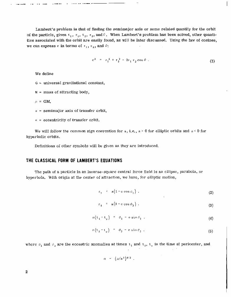
Lambert’s problem is that of finding the semimajor axis or some related quantity for the orbit of the particle, given t, , r l , t 2 , r2, and 8 . When Lambert’s problem has been solved, other quanti­ties associated with the orbit a r e easily found, as will be later discussed. Using the law of cosines, we can express c in t e rms of r l , r 2 , and 8:

We define

G = universal gravitational constant,

M = mass of attracting body,

P = GM,

a = semimajor axis of transfer orbit,

e = eccentricity of transfer orbit.

We will follow the common sign convention for a , i.e., a > 0 for elliptic orbits and a < 0 for hyperbolic orbits.

Definitions of other symbols will be given as they a r e introduced.

THE CLASSICAL FORM OF LAMBERT’S EQUATIONS

The path of a particle in an inverse-square central force field is an ellipse, parabola, or hyperbola. With origin at the center of attraction, we have, for elliptic motion,

r i = a ( l - e c 0 s 4 ~ ),

n ( t 2 - t p ) = 6,- e s i n & 2 , (5)

where 9,and b2 a r e the eccentric anomalies a t times t l and t , , t p is the time at pericenter, and

n = (,u/a3)1’2 .

2

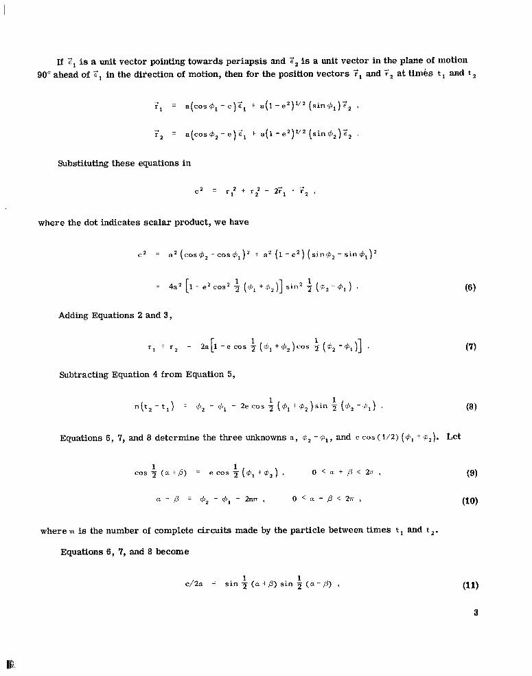
If 2, is a unit vector pointing towards periapsis and 2, is a unit vector in the plane of motion 90" ahead of Tl in the dil'ection of motion, then for the position vectors and ;2 at times t l and t ,

= a(cosc#J1- e);, + a ( 1 -e'"" ( s i n + , ) Z , ,

+r , = a ( c o s + , - e ) Z l + a ( l - e ' ) V ' ( s i n + , ) Z , .

Substituting these equations in

c 2 = r t -t r: - 27, * 7, ,

where the dot indicates scalar product, we have

c 2 = a2 (cos+2 - cos + 1 ) 2 -t a2 ( 1 - e') ( s in+ ' - s i n 4,)'

= 4a2 [I- e2 cos2 21 (b1+ +, )]s i n 2 21 ( + 2 - 9,) .

Adding Equations 2 and 3,

1 1r l + r , = 2a[l - e cos 3 ( + 1 + + 2 ) c o s 2 ( + 2 - + 1 ) ] .

Subtracting Equation 4 from Equation 5,

Equations 6, 7, and 8 determine the three unknowns a , 92- and e COS (1/2) ( + 1 + 4,). Let

where m is the number of complete circuits made by the particle between times t l and t , .

Equations 6 , 7, and 8 become

P

(0, -2lT

I Figure 1.

where we have defined

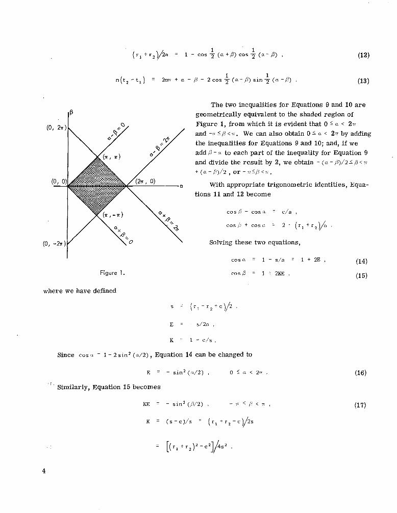
The two inequalities for Equations 9 and 10 a r e geometrically equivalent to the shaded region of Figure 1, from which it is evident that 0 a < 2 n and -n(P <n. We can also obtain 0 5 a < 271by adding the inequalities for Equations 9 and 10; and, i f we add P - a to each part of the inequality for Equation 9 and divide the result by 2, we obtain - ( a - P ) / 2 5 p < T

+ ( a - P ) / 2 , o r - n ( p < n .

With appropriate trigonometric identities, Equa­tions 11and 12 become

c o s p - cosu = c/a ,

c o s b + c o s a 2 - ( r l +r2)/a .

Solving these two equations,

cosu = 1 - s/a = 1 + 2E ,

c o s p = 1 + 2KE ,

E = - s/2a ,

K 1 - c / s .

Since cos a = 1- 2 s in’ ( a / 2 ) , Equation 14 can be changed to

E = - s i n ’ ( a / 2 ) , 0 5 a < 2 n .

. . Similarly, Equation 15 becomes

KE = - s i n 2 (P/z) , - 7 7 5 p < v ,

4

Introducing Equation 1,we have

K = ( r l r2 /2s2 ) (1 + c o s S )

= (r, r2/s*)cos2 ( ~ / 2 ) .

Substituting Equation 16 in Equation 17,

s i n (p/2) = q s i n (a/2) , - 7 r s p < 7 r ,

where

9 = * 7% = [ ( r , r*)1/2/5] cos (8/2)

Note that the sign of q is taken care of by the angle 0 :

We can introduce E into Equation 13, since

“ ( t , - t , ) = ( w / z I ~ ) ” ~( t , - t , ) = ( - E ) 3 ’ 2 T ~

where

T = ( ~ w / s ) ” ~( t , - t l ) /s .

This can also be written as

T = (-E)-3’2 [ 2 m 7 r + a - p - ( s i n a - s i n / J ) ] .

Substituting Equation 16 into Equation 22,

T s i n J ( a / 2 ) = 2 m + a - p - s i n a + s i n p

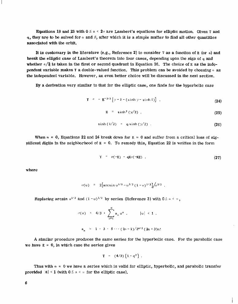
Equations 18 and 23 with 0 5 a < 27r a r e Lambert's equations for elliptic motion. Given T and 9, they arp to be salved for a and P, after which i t is a simple matter to find all other quantities a$soc/ated with the orbjt.

It is cpstomary in the literature (e.g., Reference 2) to consider T as a function of E (or a) and break the ellintic case of Lambert's theorem into four cases, depending upon the sign of q and whether a/q is taken in the first o r second quadrant in Equation 16. The choice of E as the indp­pendent variable makes T a double-valued function. This problem can be avoided by choosing a as the independent variable. However, an even better choice willbe discussed in the next section.

By a derivation very similar to that for the elliptic case, one finds for the hyperbolic case

E = s i n h 2 ( y / 2 ) , (25)

When m = 0, Equations 22 and 24 break down for E = 0 and suffer from a critical loss of sig­pificant dig-@ in the neighborhood of E = 0. To remedy this, Equation 22 is written in the form

T = a(-E) - qKa(-KE) , (27)

where

Replacing arcsin u112 and (1 - u)l12 by ser ies (Reference 3) with 0 5 a < 7r,

A similar proaedure produces the same ser ies for the hyperbolic case. For the parabolic case we have E = 0, in which case the ser ies gives

Thus with m = 0 we have a ser ies which is valid for elliptic, hyperbolic, and parabolic transfer provided ]El < 1 (with 0 5 a < 7r for the elliptic case),

6

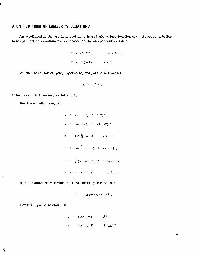
A UNIFIED FORM OF LAMBERT’S EQUATIONS

As mentioned in the previous section, T is a single-valued function of a . However, a better-behaved function is obtained if we choose as the independent variable

x = cos ( d 2 ) , - 1 5 x 5 1 ,

We then have, for elliptic, hyperbolic, and parabolic transfer,

i f for parabolic transfer, we let x = 1.

For the elliptic case, let

y = s i n ( a / 2 ) = ( - ~ ) ‘ / 2 ,

7. = cos ( P / 2 ) = (1 + K E ) ” 2 ,

1h = 3 ( s i n a - s inp) = y ( x - q z ) ,

A = a r c t a n ( f / g ) , O 5 A l n .

It then follows from Equation 21 for the elliptic case that

T = 2 ( m t A - h)/y3

For the hyperbolic case, let

7

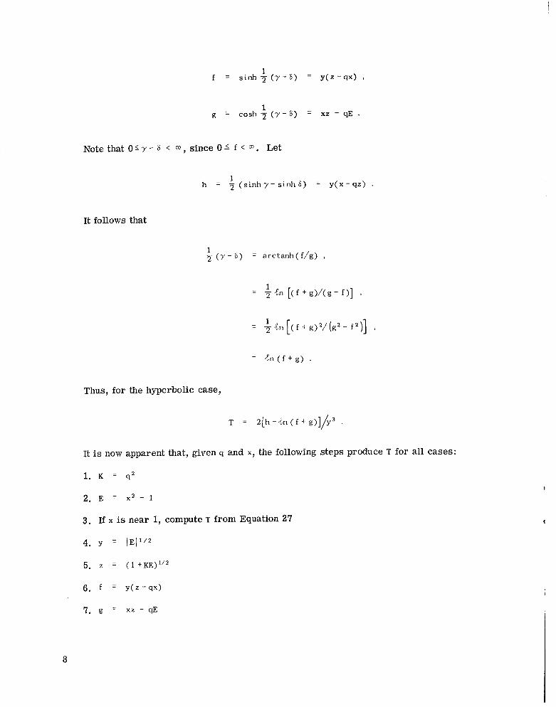
1 f = s i n h 2 ( y - S ) = y ( z - q x ) ,

1 g = cosh 3 ( y - 8 ) = xz - qE .

Note that O’Y - 6 < m, since 0’ f < a. Let

1 h = 2 ( s i n h y - s i n h 6 ) = y ( x - q z ) .

It follows that

1 ( y - 8 ) = a r c t a n h ( f/g) ,

Thus, for the hyperbolic case,

T = 2[h - i n ( f + g)]/y3

It is now apparent that, given q and x, the following steps produce T for all cases:

1. K = q 2

2. E = x z - 1

3. If x is near 1, compute T from Equation 27

4. Y = lE11/2

5. z = ( 1 ~ K E ) ” ~

6. f = ~ ( z - q x )

7. g = xz - qE

8

9. T = 2 ( x - qz -d/y)/E.

The following formula for the derivative holds for all cases except for x = 0 with K = 1, and for x = 1:

dT/dx = ( 4 - 4qKx/z - 3xT)/E .

If x is near 1, differentiate Equation 27 to obtain

dT/dx = 2x[qK2 c'(-KE) -0 ' (-E)] ,

m

~ ' ( u ) = du/du = z n a n u n - '

"= 1

The derivative in the case of x = 0 with k = 1will be discussed in the next section.

AUXILIARY FORMULAS

In this section we will show how to obtain a number of useful quantities associated with the two-body orbit, assuming Lambert's problem has been solved for x.

In the derivation of Lambert's equation for the elliptic case, J. and .A+ a r e defined in such a way that

4, - .p, a - ,A t 2 m = 2(X + m ) .

From Equation 22, the eccentric anomaly difference can also be written in the form

d', - = ( - E ) 3 ' 2 T + s i n a - s i n p

= y 3 T + 2 y ( x - q z )

From Equation 28 we have

9

4,.- - s i n (4,- = y 3 T - 4y3 q(z - 9x1 , (29)

1 - cos(q52-q51) = 2yZ(z-qx)Z . (3 0)

We now obtain a formula for the time derivative i at time t 1. Kepler’s equation in the elliptic case can be written in the form (Reference 4)

Substituting l / a = 2 y 2 / s , t, - t, = s3/’ T/(~P)”* ,and making use of Equations 29 and 30 gives

( 2 / p ~ ) ~ ” ( z - q x )r l ;, = 2q - ( 2 r l / s ) ( x z - q E ) .

Multiplying through by z + qx, we have, since ( z - qx) ( z + qx) = 1 - K = c/s and ( z + qx) ( x z - qE)

x + q z ,

( ~ / , L L S ) ~ / ~ C ~ , ; ~= 2 q s ( z + q x ) - 2 r l ( x + q z )

= 2 q z ( s - r l ) + 2 x ( K s - r l ) ;

K s - r l = ( l - c / s ) s - r l s - c - r l = r , - s

Thus we have finally that

At time t , we find

By a similar procedure we can show that Equations 3 1 and 3 2 hold also for the hyperbolic and parabolic cases.

Having X , we can find the semimajor axis a , or its reciprocal,

10

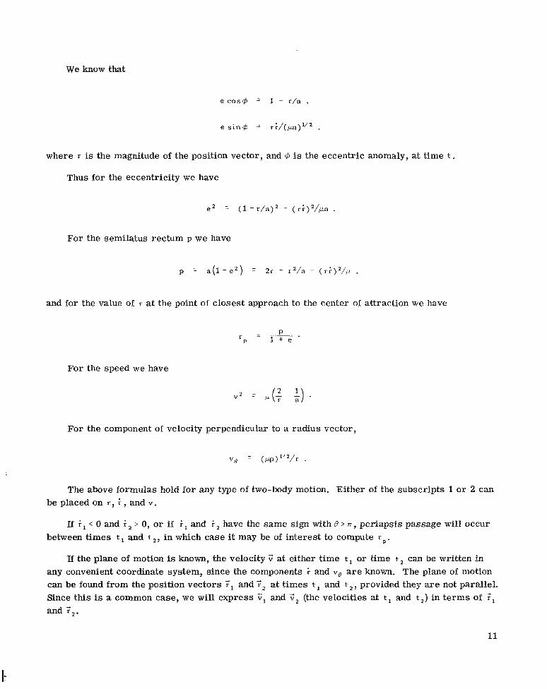
We know that

where r is the magnitude of the position vector, and 4 is the eccentric anomaly, at time t ,

Thus for the eccentricity we have

For the semilatus rectum P we have

and for the value of r at the point of closest approach to the center of attraction we have

For the speed we have

“ 2 = & -a, .

For the component of velocity perpendicular to a radius vector,

= (pp)”‘/r

The above formulas hold for any type of two-body motion. Either of the subscripts 1 or 2 can be placed on r , i ,and V.

If i, < 0 and i, > 0, or if i, and i, have the same sign with B > n , periapsis passage will occur between times t ,and t 2 , in which case it may be of interest to compute r p .

If the plane of motion is known, the velocity 5 at either time t ,or time t can be written in any convenient coordinate system, since the components i and vQ a r e known. The plane of motion can be found from the position vectors and 2’ at times t ,and t ’, provided they are not parallel. Since this is a common case, we will express 2 , and i;, (the velocities at t l and t,) in t e rms of y1 and 2‘.

11

- - -

- - -

For the velocity G1 we have

where G r l is along T1 and Gel is in the plane of motion perpendicular to ;1 and in the direction of motion, Le., in the direction of increasing true anomaly. We have

where c1 and c, a r e to be determined.

r l . vO1 ­

r~ . -

Figure 2.

+ *o = c1 r: + c, r l . r ,

+ + r , vO1s i n @ = c1 r l e r 2 + c 2 r g

r l c 1 + ( r , cos B ) C , = o ,

( r l c o s @ )c1 + r 2 c , = ve s i n 0 .

Solving for c1 and c 2 , we have

In a similar way, we find

Figure 2 shows T as a function of X . Note the discontinuity in the slope for x = 0 with K = 1. ForK = 1, z = 1x1. Thus w e a r e l e d to consider four cases: q = 51 with x 2 0, q = r t l with x 5 0. Examination of the formulas for dT/dx in these cases reveals that i f q = 1 we have a left-hand derivative of -8 and a right-hand derivative of 0 at x = 0. If q = -1 we have a left-hand derivative of 0 and a right-hand derivative of -8 at x = 0.

12

With further analysis we find that the cases (q = 1, x 5 0)and (q = -1, x 2 0) represent recti­linear orbits.

For m = 0, T is a monotone function of x, making possible a simple numerical procedure for solving Lambert's problem. Figure 2 is for the elliptic case, Figure 3 for the hyperbolic case, the parabolic case occurring at x = 1in both figures. Figure 4 shows a small region of Figure 2

9 0 " , I I

1 1.2 'i 1.4 1.6 1.8 2 X

e.

Figure 3.

where d2 T/dx2 is negative. If the Newton-Raphson method is being used to find x , a switch should be made in this region to the se­cant (regula falsi) method.

No solutions of Lambert's problem exist +

in the shaded regions of Figures 2 and 3. x = 1 (m > 0) and x = -1 a r e vertical asymp­totes. T - 0 as X - - J J .

Goddard Space Flight Center -0.20 -0.15 -0.10 -0.05 0 0.05 0.10 0.15 0.20 National Aeronautics and Space Administration X

Greenbelt, Maryland, May 28, 1969 188-48-01-05-5 1 Figure 4.

REFERENCES

1. Lancaster, E. R., Blanchard, R. C., and Devaney, R. A., "A Note on Lambert's Theorem," 7 Joumal of Spacecvaft and Rockets 3 (9):1436-1438, September 1966.

2. Breakwell, John V., Gillespie, Rollin W., and Ross, Stanley, "Researches in Interplanetary Transfer,' ' ARS J. 31:201-208, February 1961.

3. Gedeon, G. S., "Lambertian Mechanics,'' Proceedings of the X I t h Intevnntio?zal Astvonautical Congress (Springer-Verlag, Wien, and Academic P res s Inc., New York, 1963).

4. Battin, Richard H., "Astronautical Guidance," New York: McGraw-Hill Book Co., Inc., 1964, page 46.

13 NASA-Langley, 1969 -30

NATIONAL AND SPACE ADMINISTRATIONAERONAUTICS WASHINGTON,D. C. 20546

OFFICIAL BUSINESS FIRST CLASS MAIL

POSTAGE AND FEES PAID NATIONAL AERONAUTICS A N D

SPACE ADMINISTRATION

If Undelivtrdble (Section 156 Postal Manual) Do Not Return

“The aerotzrutticnl niad space nrtii’ities of ihe United Stntes shnll be . coizditcted so ns to coiztribute . . . t o the expnnsion of hitiiiaia kia01~1­

edge of pheuotiieizn iia the ntiiiosphere nizd spnce. The Adiiiiiaistratioiz shrill proi fide fo r the widest prncticnble ntzd nppropsinte disseiiiim!io?z . of iiiforiiintioiz coiicerizing its rrctiimitirs nitd the resnlts thereof.”

-NATIONALAERONAUTICSA N D SPACE ACT OF 1358

NASA SCIENTIFIC AND TECHNICAL PUBLICATIONS

TECHNICAL REPORTS: Scientific and technical information considered important, complete, and a lasting contribution to existing knowledge.

TECHNICAL NOTES: Inforrnation less broad in scope but nevertheless of importance as a contribution to existing knowledge.

TECHNICAL MEMORANDUMS: Information receiving limited distribution because of preliminary data, security classifica­tion, or other reasons.

CONTRACTOR REPORTS: Scientific and technical information generated under a NASA contract or grant and considered an important contribution to existing knowledge.

TECHNICAL TRANSLATIONS: Information published in a foreign language considered to merit NASA distribution in English.

SPECIAL PUBLICATIONS: Information derived from or of value to NASA activicies. Publications include conference proceedings, monographs, data compilations, handbooks, sourcebooks, and special bibliographies.

TECHNOLOGY UTILIZATION PUBLICATIONS: Information on technology used by NASA that may be of particular interest i n cornrnercial and other non-aerospace npplications. Publications include Tech Briefs, .,-echnctlogy Util ization Reports and Notes, and Technology Surveys.

Details on the availability of these publications may be obtained from:

SCIENTIFIC AND TECHNICAL INFORMATION DIVISION

NATI0NA L AERO NAUT1C S AND SPACE ADM INISTRATI0N Washington, D.C. 20546