Theory of Computing Systems manuscript No.(will be inserted by the editor)

Nash Equilibria and the Price of Anarchy for Flows Over

Time

Ronald Koch · Martin Skutella

Received: date / Accepted: date

Abstract We study Nash equilibria in the context of flows over time. Manyresults on static routing games have been obtained over the last ten years.In flows over time (also called dynamic flows), flow travels through a networkover time and, as a consequence, flow values on edges are time-dependent. Thismore realistic setting has not been tackled from the viewpoint of algorithmicgame theory yet; but there is a rich literature on game theoretic aspects offlows over time in the traffic community.

We present a novel characterization of Nash equilibria for flows over time.It turns out that Nash flows over time can be seen as a concatenation of specialstatic flows. The underlying flow over time model is the so-called deterministicqueuing model that is very popular in road traffic simulation and related fields.Based upon this, we prove the first known results on the price of anarchy forflows over time.

Keywords Flow over time · Nash equilibrium · Routing game · Deterministicqueuing model

1 Introduction

In a groundbreaking paper, Roughgarden and Tardos [42] (see also Roughgar-den’s book [41]) analyze the price of anarchy for selfish routing games in net-works. Such routing games are based upon a classical static flow problem withconvex latency functions on the edges of the network. In a Nash equilibrium,flow particles (infinitesimal flow units) selfishly choose an origin-destinationpath of minimum latency.

Supported by DFG Research Center Matheon “Mathematics for key technologies” in Berlin.An extended abstract of this work has been presented at the 2nd International Symposiumon Algorithmic Game Theory, see [25].

TU Berlin, Inst. f. Mathematik, MA 5-2, Str. des 17. Juni 136, 10623 Berlin, GermanyE-mail: koch,skutella@math.tu-berlin.de

2

One main drawback of this class of routing games is its restriction to staticflows. Flow variation over time is, however, an important feature in networkflow problems arising in various applications. As examples we mention roador air traffic control, production systems, communication networks (e. g., theInternet), and financial flows; see, e. g., [5,37]. In contrast to static flow models,flow values on edges may change with time in these applications. Moreover,flow does not progress instantaneously but travels at a certain pace throughthe network which is determined by transit times on the edges. Both temporalfeatures are captured by flows over time (sometimes also called dynamic flows)which were introduced by Ford and Fulkerson [15,16].

Another crucial phenomenon in many of those applications mentionedabove is the variation of time taken to traverse an edge with the current (andmaybe also past) flow situation on this edge. The latter aspect induces highlycomplex dependencies and leads to non-trivial mathematical flow models. Fora more detailed account and further references we refer to [5,11,19,30,37,38].In particular, all of these flow over time models have so far resisted a rigorousalgorithmic analysis of Nash equilibria and the price of anarchy.

We identify a suitable flow over time model that is based on the followingsimplifying assumptions. Every edge of a given network has a fixed free flowtransit time and a capacity. The capacity of an edge bounds the rate (flow pertime unit) at which flow can leave this edge. The free flow transit time denotesthe time that a flow particle needs to travel from the tail to the head of theedge. If, at some point in time, more flow wants to traverse an edge than itscapacity allows, the flow particles queue up at the end of the edge and wait inline before they actually enter the head node. When a new flow particle wantsto traverse an edge, the time needed to arrive at the head thus consists of thefixed free flow transit time plus the waiting time. In the traffic literature, thisflow over time model is known as deterministic queuing model.

Related Literature. Flows over time with fixed transit times were introducedby Ford and Fulkerson [15,16]. For more details and further references on theseclassical flows over time we refer, for example, to [14,43].

So far, Nash equilibria for flows over time were mostly studied within thetraffic community. Vickrey [48] and Yagar [51] are the first to introduce thistopic. Up to the middle of the 1980’s, nearly all contributions consider Nashequilibria on given small instances; see, e. g., [21,29,35,48]. Since then, thenumber of publications in this area has increased rapidly and Nash equilib-ria were modeled mathematically. Two main models are distinguished: Theroute-choice-model where a player only chooses an s-t-path for the controlledflow particle and the simultaneous departure-time-route-choice-model where inaddition the departure time is also chosen. For a survey see, e. g., [36]. Theconsidered models can be grouped into four categories: mathematical pro-gramming (e. g., [20,28]), optimal control (e. g., [18,39]), variational inequal-ities (e. g., [12,17,40,45,46]), and simulation-based approaches (e. g., [7,6,31,47,51]). Up to now, variational inequalities are the most common formulationfor analyzing Nash equilibria in the context of flows over time.

3

Many models mentioned above use a path-based formulation of flows overtime. Therefore they are often computationally intractable. Edge-based formu-lations are, for example, considered in [2,12,40]. Realistic assumptions on theunderlying flow model with respect to traffic are described by Carey [9,10].

In this paper the deterministic queuing model is considered. This model wasintroduced by Vickrey [48] and later by Hendrickson and Kocur [21]. Smith [44]shows the existence of an equilibrium for this model in a special case. Aka-matsu [1,2] presents an edge-based formulation of the deterministic queuingmodel on restricted single-source-instances. Akamatsu and Heydecker [3] studyBraess’s paradox for single-source instances. Braess’s paradox [8] states (forstatic flows) that increasing the capacity of one edge can increase the total costof all users in a Nash flow. It is well known that this paradox is extendable tothe dynamic case. Mounce [32,33] considers the case where the edge capaci-ties can vary over time and states some existence results. Again, it should bementioned that these results are based on strong assumptions.

Recently, Anshelevich and Ukkusuri [4] analyze discrete routing game mod-els for Nash equilibria in the context of flows over time. They consider howa single splittable flow unit present at source s at time 0 would traverse anetwork assuming every flow particle is controlled by a different player. Theunderlying flow model allows to send a positive amount of flow over an edgeat each integral points in time. Moreover the transit times are assumed to beconstant. Hoefer et. al [22] also consider a discrete routing game. They studyexistence and complexity properties of pure Nash equilibria and best-responsestrategies.

Our Contribution. In this paper, we characterize and analyze Nash equi-libria for flows over time. Although algorithmic game theory is a flourishingarea of research (see, e. g., the recent book [34]), network flows over time havenot been studied from this perspective in the algorithms community so far.The main purpose of this paper is to make first steps in this relevant direc-tion, present interesting and novel results, and stimulate further interestingresearch. We consider the deterministic queuing model in networks with a sin-gle source and a single sink. A player controls one flow particle and chooses ans-t-path (route-choice-model) but no departure time which is given a priori.

A precise description of a routing game over time and the underlying flowover time model is given in Section 2. The resulting model of Nash equilibriaalong with several equivalent characterizations is discussed in Section 3. Themain technical contribution of this paper is presented in Section 4. Here weshow that a Nash equilibrium can be characterized via a sequence of staticflows with special properties. The resulting static flow problems are of interestin their own right. The final Section 5 is devoted to results on the price ofanarchy. For the important class of shortest paths networks we prove that everyNash equilibrium is a system optimum. Moreover, a Nash flow over time canbe computed in polynomial time by a sequence of sparsest cut computations.Surprisingly, for arbitrary networks, the price of anarchy is not bounded by aconstant.

4

2 A model for routing games over time

In this section we present a model for Nash equilibria in the context of flowsover time. In Section 2.1 we define a routing game over time and elaborate onthe game theoretic aspect of the model. Then, in Section 2.2 we introduce anappropriate flow over time model which is known as the deterministic queuingmodel.

Throughout the paper we often use the term flow particle in order to referto an infinitesimal flow unit which corresponds to one player and travels alonga single path through the network. The terms flow rate and supply rate bothrefer to an amount of flow per time unit.

2.1 From static routing games to routing games over time

Consider a network consisting of a directed graph G := (V, E) with nodeset V and edge set E. Further, there is a source s ∈ V and a sink t ∈ V .Each flow particle is a player and the strategy set of each player is the set Pof all s-t-paths.

In a static routing game, the players’ decisions yield a static s-t-flow µ ofvalue d where d is the given supply at the source s. Moreover, there is a contin-uous cost (or payoff) function ℓP for each path P ∈ P such that ℓP (µ) is thecost that a player choosing path P has to pay. The static flow µ = (µP )P∈P is aNash flow if, for all P ∈ P with µP > 0, it holds that ℓP (µ) = minP ′∈P ℓP ′(µ).

The situation is considerably more complicated when we turn to routinggames over time. Here we assume that supply, i. e., players, occur at the sourcenode s over time at a fixed rate d. We can thus identify each player with thepoint in time θ at which its corresponding flow particle originates at the source.In particular, and in contrast to static routing games, players are not identical.The routing decisions of players yield a flow over time µ = (µP )P∈P whereµP is a function determining the flow rate µP (θ) at which flow enters path Pat time θ and it holds that

∑P∈P µP (θ) = d, for all θ. Thus, also ℓP (µ) is a

function which assigns a cost ℓP (µ)(θ) to every point in time θ. That is, thecost experienced by a flow particle that originates at the source at time θ andchooses path P is equal to ℓP (µ)(θ).

In this paper we restrict to cost functions where ℓP (µ)(θ), P ∈ P , is thetime when a flow originating at s at time θ arrives at the sink t. This timedepends upon the particular model of flows over time that we consider whichis described in Section 2.2 below.

Like in static routing games, a Nash equilibrium is characterized by a flowover time µ where no player has an incentive to change her chosen path inorder to reduce her cost.

Definition 1 (Nash flow over time) Let µ be a flow over time determiningthe routing decisions of the players in a routing game over time. Then, µ is aNash equilibrium (Nash flow over time) if, for almost all θ and for all P ∈ Pwith µP (θ) > 0, it holds that ℓP (µ)(θ) = minP ′∈P ℓP ′(µ)(θ).

5

This definition is an immediate generalization of the definition of staticNash flows under the assumption that the payoff functions are continuous. Acloser look at Definition 1 shows that the continuity of the payoff functions ℓP

is also essential here since it ensures the following. If an actual routing µ doesnot fit Definition 1, then some measurable set of players must have an incentiveto switch to a path P of minimum latency. Hence, the switching of the playersmust not imply a large increase of the payoff function ℓP .

2.2 An appropriate flow over time model

Although Definition 1 is an immediate generalization of static Nash flows, itis still a highly nontrivial problem to come up with an appropriate flow overtime model. Here the main issue are the cost functions ℓP , P ∈ P . For staticrouting games, these cost functions are not given explicitly, but implicitly viaedge latency functions. The cost of a path P ∈ P is the sum of the latenciesof its edges. The latency of an edge e is a function of the load µe of that edgewhich can easily be computed as follows: µe :=

∑P∈P:e∈E(P ) µP .

The situation is considerably more complicated for flows over time. Here,it is usually a highly nontrivial problem to compute the flow rate function µe

of edge e from given flow rate functions (µP )P∈P . Consider a flow particlethat enters a path P ∈ P at a certain time θ. Notice that the time at whichthis particle arrives at an edge e ∈ E(P ) depends on the latencies experiencedon the predecessor edges on path P . This fact induces involved dependenciesamong the flow rate functions (µe)e∈E of the edges. As a consequence, givena flow over time (µP )P∈P , determining the cost (overall latency) of a flowparticle entering path P at time θ is, in general, a highly nontrivial task.For more details on this so-called dynamic network loading problem we referto [49,50]. Nevertheless, for the deterministic queuing model described below,these difficulties can be handled at least for the case of Nash flows over time.

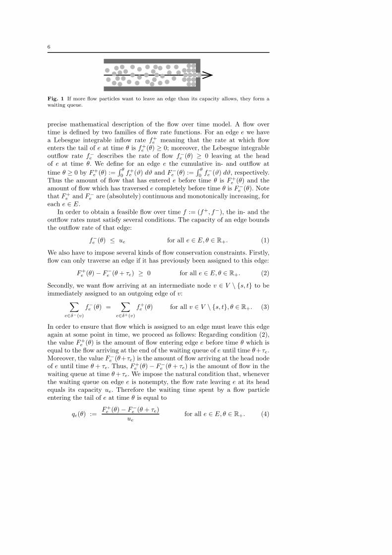
Let (G, u, τ, s, t) be a network consisting of a directed graph G := (V, E),edge capacities ue ∈ R+, e ∈ E, constant free flow transit times τe ∈ R+,e ∈ E, a source s ∈ V , and a sink t ∈ V . We assume without loss of generalitythat there are no incoming edges at the source s and no outgoing edges at thesink t and that every node v is reachable from s. The capacity ue of an edge ebounds the rate at which flow leaves edge e at its head node. The basic conceptof the considered flow over time model are waiting queues which build up atthe head (exit) of an edge if, at some point in time, more flow particles want toleave an edge than the capacity of the edge allows. The free flow transit timeof an edge determines the time for traversing an edge if the waiting queue isempty. Thus, the (flow-dependent) transit time on an edge is the sum of thefree flow transit time and the current waiting time. We think of the edges ascorridors with large entries and small exits, which are wide enough for storingall waiting flow particles (point-queue-model); see Fig. 1.

Every flow particle arriving at an intermediate node v immediately entersthe next edge on its path without any delay. In the following we give a more

6

Fig. 1 If more flow particles want to leave an edge than its capacity allows, they form awaiting queue.

precise mathematical description of the flow over time model. A flow overtime is defined by two families of flow rate functions. For an edge e we havea Lebesgue integrable inflow rate f+

e meaning that the rate at which flowenters the tail of e at time θ is f+

e (θ) ≥ 0; moreover, the Lebesgue integrableoutflow rate f−

e describes the rate of flow f−e (θ) ≥ 0 leaving at the head

of e at time θ. We define for an edge e the cumulative in- and outflow at

time θ ≥ 0 by F+e (θ) :=

∫ θ

0 f+e (ϑ) dϑ and F−

e (θ) :=∫ θ

0 f−e (ϑ) dϑ, respectively.

Thus the amount of flow that has entered e before time θ is F+e (θ) and the

amount of flow which has traversed e completely before time θ is F−e (θ). Note

that F+e and F−

e are (absolutely) continuous and monotonically increasing, foreach e ∈ E.

In order to obtain a feasible flow over time f := (f+, f−), the in- and theoutflow rates must satisfy several conditions. The capacity of an edge boundsthe outflow rate of that edge:

f−e (θ) ≤ ue for all e ∈ E, θ ∈ R+. (1)

We also have to impose several kinds of flow conservation constraints. Firstly,flow can only traverse an edge if it has previously been assigned to this edge:

F+e (θ) − F−

e (θ + τe) ≥ 0 for all e ∈ E, θ ∈ R+. (2)

Secondly, we want flow arriving at an intermediate node v ∈ V \ s, t to beimmediately assigned to an outgoing edge of v:

∑

e∈δ−(v)

f−e (θ) =

∑

e∈δ+(v)

f+e (θ) for all v ∈ V \ s, t, θ ∈ R+. (3)

In order to ensure that flow which is assigned to an edge must leave this edgeagain at some point in time, we proceed as follows: Regarding condition (2),the value F+

e (θ) is the amount of flow entering edge e before time θ which isequal to the flow arriving at the end of the waiting queue of e until time θ+τe.Moreover, the value F−

e (θ+τe) is the amount of flow arriving at the head nodeof e until time θ + τe. Thus, F+

e (θ) − F−e (θ + τe) is the amount of flow in the

waiting queue at time θ + τe. We impose the natural condition that, wheneverthe waiting queue on edge e is nonempty, the flow rate leaving e at its headequals its capacity ue. Therefore the waiting time spent by a flow particleentering the tail of e at time θ is equal to

qe(θ) :=F+

e (θ) − F−e (θ + τe)

ue

for all e ∈ E, θ ∈ R+. (4)

7

The interpretation of qe(θ) as the waiting time for flow particles arriving attime θ on edge e is based on the assumption that the first-in-first-out (FIFO)property holds on edge e. That is, no flow particle overtakes any other flowparticle within the waiting queue. Since the free flow transit times are constant,the FIFO property holds for the entire edge.

Proposition 1 For any edge e ∈ E, the following statements are valid:

(i) The function θ 7→ θ + qe(θ) is monotonically increasing and continuous.(ii) F+

e (θ) = F−e

(θ + τe + qe(θ)

)for all θ ∈ R+.

(iii) Consider two points in time θ2 > θ1 ≥ 0 such that∫ θ2

θ1f+(ϑ) dϑ = 0 and

qe(θ2) > 0. Then we have θ1 + qe(θ1) = θ2 + qe(θ2).

Proof Let θ2 > θ1 ≥ 0. For proving (i) note that F−e (θ2 + τe) − F−

e (θ1 +τe) ≤ ue(θ2 − θ1) because of (1). Hence qe(θ1) − qe(θ2) ≤ θ2 − θ1 is impliedby F+

e (θ1) − F+e (θ2) ≤ 0 and (4). The continuity follows from (4) and the

continuity of F+e and F−

e .Since we assume that, whenever the waiting queue on edge e is nonempty,

the flow rate leaving e at its head equals the capacity ue, statement (ii) isdirectly implied by (4).

It remains to prove statement (iii). Since we have F+e (θ1) = F+

e (θ2), weobtain F+

e (θ′) = F+e (θ2) for all θ′ ∈ [θ1, θ2) because F+

e is monotonicallyincreasing. Since F−

e is also monotonically increasing and qe(θ2) > 0, this im-plies F+

e (θ′) − F−e (θ′ + τe) ≥ F+

e (θ2) − F−e (θ2 + τe) > 0 for all θ′ ∈ [θ1, θ2).

Hence, there is a nonzero waiting queue on e for all times in [θ1, θ2), imply-ing that f−

e is equal to ue for all times in [θ1, θ2). Thus, we conclude thatqe(θ1) − qe(θ2) = θ2 − θ1. ⊓⊔

As already mentioned, the flow-dependent transit time τe(θ) experienced byflow particles entering e at time θ is τe(θ) := τe+qe(θ). Note, that the mappingf+

e 7→ τe, which maps an inflow rate f+e to the transit time function τe, is

continuous. This is due to the fact that additional flow of value ǫ > 0 can causeat most an additional delay of ǫ

ue. Therefore, for the case of the deterministic

queuing model, a Nash equilibrium of a routing game over time is well-definedin terms of Definition 1.

3 Characterizing Nash flows over time

The main aspect of Nash equilibria in flow models is the selfish routing of flowparticles which are identified with players. As mentioned in Section 2.1, weassume that flow occurs at the source s according to a fixed supply rate d ∈ R+.As soon as a flow particle pops up at the source, it decides by itself how totravel to the sink t. That is, it chooses an s-t-path and immediately enters thefirst edge of that path.

We consider two – apparently related – classes of flows over time. In thefirst class, every flow particle travels along “currently shortest paths” only.

8

In the second class, every flow particle tries to overtake as many other flowparticles as possible while not being overtaken by others. It turns out that thelatter condition leads to a flow where no particle overtakes any other particle.Moreover, we show that the two classes of flows over time coincide and are, infact, Nash flows over time.

We start by defining currently shortest s-t-paths in a given flow over time.To do so, we consider the problem of sending an additional flow particle attime θ ≥ 0 from the source s to the sink t as quickly as possible. Let ℓv(θ) bethe earliest point in time at which this flow particle can arrive at node v ∈ V .Then,

ℓv(θ) + τe + qe(ℓv(θ)) ≥ ℓw(θ) for each e = vw ∈ E. (5)

On the other hand, for each node w ∈ V \ s, there exists at least oneincoming edge e = vw ∈ δ−(w) such that equality holds in (5). That is, theflow particle can use edge e in order to arrive at node w as early as possible,i. e., at time ℓw(θ). Moreover, we have ℓs(θ) = θ for all θ ≥ 0. Therefore, wedefine the label functions ℓw : R+ → R+ as follows:

ℓw(θ) :=

θ for w = s,

mine=vw

ℓv(θ) + τe + qe(ℓv(θ)) for w ∈ V \ s.(6)

The label functions can be computed simultaneously for all times θ by adaptingthe shortest path algorithm of Bellman and Ford1. The next proposition followsfrom (6) and Proposition 1.

Proposition 2 For each node v ∈ V , the label function ℓv is monotonicallyincreasing and continuous.

Before proceeding with the main discussion of this section, we first con-sider an intuitive real-world example. This example will also illustrate thesubsequent definitions and results.

Example 1 Suppose you are at the airport and, since you are already late, youwant to get to your departure gate as quickly as possible. But first you haveto check-in. Afterwards, you head for the security check in order to finally getto your gate and board the aircraft. But there is a waiting queue in front ofthe check-in counter. The question is how quickly you should approach theend of the waiting queue at the check-in counter. Of course, as long as the lastperson in line remains the same, i. e., no one else enters the line, it does notmatter at what time you line up – you always leave the check-in counter at thesame time. However, if there are people behind you who want to check in atthe same counter, they could overtake you if you do not line up immediately.

1 The update procedure of Bellman-Ford for a certain label ℓw(θ) is applied for all times θ

simultaneously and, hence, is seen as an operation on functions. If we use Dijkstra’s algorithminstead, we have to maintain the set of already finalized nodes separately for each time θ.Thus, we also have to apply the update procedure of Dijkstra separately for each θ.

9

In a Nash equilibrium, flow should always be sent over currently short-est s-t-paths only. We say that edge e ∈ E is contained in a shortest pathat time θ ≥ 0 if and only if ℓw(θ) = ℓv(θ) + τe + qe(ℓv(θ)). Of course, if anedge e = vw ∈ E does not lie on a shortest s-t-path at a certain time θ ≥ 0,then no flow should be assigned to that edge at time ℓv(θ) in a Nash flow.

Definition 2 We say that flow is only sent along currently shortest pathsif, for each edge e = vw ∈ E, the following condition holds for almost alltimes θ ≥ 0:

ℓw(θ) < ℓv(θ) + τe + qe(ℓv(θ)) =⇒ f+e (ℓv(θ)) = 0 .

We emphasize the following aspect of a routing satisfying Definition 2: In astatic shortest path all subpaths are also shortest paths if the transit timesare positive. But this is no longer true if we consider the dynamic case asillustrated in Example 1. Here, as long as the last person in line remains thesame you always leave the check-in counter at the same time. So, in principle,you could decide to make a detour – maybe for buying a small present foryour family – and you can still leave the check-in counter as early as possible.However, in this case you will use at least one edge which does not lie on acurrently shortest path. Since Definition 2 forbids entering that edge, you haveto line up at the check-in counter as early as possible

As we see below the condition in Definition 2 is equivalent to the conditionthat every particle tries to overtake as much other flow as possible while notbeing overtaken. The latter condition is in fact a universal FIFO condition.That is, it is equivalent to the statement that no flow particle can possiblyovertake any other flow particle.

In order to model the universal FIFO condition more formally, we consideragain an additional flow particle originating at s at time θ ≥ 0. Of course, inorder to ensure that no flow particle has the possibility to overtake this particle,it is necessary to take a shortest s-t-path. Therefore, for each edge e = vw ∈ E,we define the amount of flow x+

e (θ) assigned to e before this particle can reach vand the amount of flow x−

e (θ) leaving e before this particle can reach w asfollows:

x+e (θ) := F+

e (ℓv(θ)) , x−e (θ) := F−

e (ℓw(θ)) for all θ ≥ 0. (7)

Thus, the amount of flow bs(θ) := d · θ that has originated at s before our flowparticle occurs at s and the amount of flow −bt(θ) arriving at t before our flowparticle can reach t satisfy

bs(θ) =∑

e∈δ+(s)

x+e (θ) and bt(θ) = −

∑

e∈δ−(t)

x−e (θ) . (8)

By definition, bs(θ) is always nonnegative and bt(θ) is always non-positive.If bs(θ) > −bt(θ), then the considered flow particle overtakes other flow par-ticles. And if bs(θ) < −bt(θ), then the flow particle is overtaken by other flowparticles. This motivates the following definition.

10

Definition 3 We say that no flow overtakes any other flow if, for each pointin time θ ≥ 0, it holds that bs(θ) = −bt(θ).

Intuitively, this definition must be satisfied by a Nash flow over time: Assumethat a flow particle p2 originating at the source at time θ2 overtakes an earlierflow particle p1 originating at the source at time θ1 < θ2. That is, p2 arrivesat the sink before p1. Because the function θ 7→ θ + τe + qe(θ) is monotonicallyincreasing for each edge e (see Proposition 1), flow particle p1 can avoid beingovertaken by p2 and improve its cost (arrival time at the sink) by choosing thesame path as p2.

Now we are able to prove the equivalence of the universal FIFO conditionand the condition that flow only uses currently shortest paths. Further, bothconditions characterize Nash flows over time. In addition, a further equivalentcharacterization is given. With respect to Example 1, Theorem 1 also tells youwhy you should line up immediately. It says that if you do not reach the end ofthe waiting queue as early as possible, then other persons may overtake you.

Theorem 1 For a given flow over time, the following statements are equiva-lent:

(i) Flow is only sent along currently shortest paths.(ii) For each edge e ∈ E and at all times θ ≥ 0, it holds that x+

e (θ) = x−e (θ).

(iii) No flow overtakes any other flow.(iv) The given flow over time is a Nash flow over time.

In the proof of Theorem 1, the following lemma plays an important role. Itgives a more global characterization of when flow is being sent only alongcurrently shortest paths (Definition 2 gives only a pointwise characterization).

Lemma 1 For a given flow over time, the following statements are equivalent:

(i) Flow is only being sent along currently shortest paths.(ii) For each edge e = vw ∈ E and for all θ ≥ 0, it holds that

F−e

(ℓv(θ) + τe + qe(ℓv(θ))

)= F−

e

(ℓw(θ)

). (9)

Proof Equation (9) is obviously fulfilled if edge e is contained in a shortestpath at time θ. In the following, it is thus enough to consider only edges e andtimes θ such that e does not lie on a shortest path at time θ.

(i)⇒(ii): Let θ ≥ 0 and e = vw ∈ E be an edge which is not contained ina shortest path at time θ, i. e., ℓw(θ) < ℓv(θ) + τe + qe(ℓv(θ)). Let

θ1 := max0, supθ′ ≥ 0 | ℓw(θ) ≥ ℓv(θ′) + τe + qe(ℓv(θ′))

.

be the latest point in time at which a flow particle is able to arrive at w via ebefore time ℓw(θ) (and 0 if no such point in time exists). By definition of θ1,

ℓw(θ′) ≤ ℓw(θ) < ℓv(θ′) + τe + qe(ℓv(θ

′)) for all θ′ ∈ (θ1, θ].

11

Thus, edge e does not occur in a shortest path within the time interval (θ1, θ].Because of Definition 2 and Proposition 1(ii), we get

0 = F+e

(ℓv(θ)

)− F+

e

(ℓv(θ1)

)

= F−e

(ℓv(θ) + τe + qe(ℓv(θ))

)− F−

e

(ℓv(θ1) + τe + qe(ℓv(θ1))

).

(10)

Equation (10) implies (ii) because

ℓv(θ1) + τe + qe(ℓv(θ1)) ≤ ℓw(θ) < ℓv(θ) + τe + qe(ℓv(θ))

and because F−e is monotonically increasing.

(ii)⇒(i): Let θ ≥ 0 and e = vw ∈ E an edge that is not contained in ashortest path at time θ, i. e., ℓw(θ) < ℓv(θ) + τe + qe(ℓv(θ)). By Propositions 1and 2, there exists an ǫ > 0 such that ℓw(θ + ǫ) < ℓv(θ− ǫ)+ τe + qe(ℓv(θ− ǫ)).Thus, the nonnegativity of the flow rate functions yields:

0 ≤

∫ ℓv(θ+ǫ)

ℓv(θ−ǫ)

f+e (ϑ) dϑ =

∫ ℓv(θ+ǫ)+τe+qe(ℓv(θ+ǫ))

ℓv(θ−ǫ)+τe+qe(ℓv(θ−ǫ))

f−e (ϑ) dϑ

≤

∫ ℓv(θ+ǫ)+τe+qe(ℓv(θ+ǫ))

ℓw(θ+ǫ)

f−e (ϑ) dϑ = 0 .

This yields statement (i). ⊓⊔

Within the proof of Theorem 1 we construct a static b-flow. For convenienceof the reader, we give the definition of b-flows here (for more details we referto [27]).

Definition 4 Let H be a graph with node set V (H) and edge set E(H) andb′v ∈ R be a real value for each node v ∈ V (H). The supply-demand vector(b′v)v∈V (H) has to satisfy

∑v∈V (H) b′v = 0. A static flow x′ := (x′

e)e∈E(H) ∈

RE(H)+ is called b′-flow if it satisfies the flow conservation constraint

∑

e∈δ+(v)

x′e −

∑

e∈δ−(v)

x′e = b′v for each v ∈ V (H).

If in addition, for each edge e ∈ E(H), an edge capacity ue ∈ R is given, afeasible b-flow has to satisfy x′

e ≤ ue for each e ∈ E(H).

Proof (of Theorem 1) The main observation we need is the following equationwhich we get from Proposition 1(ii) and the definitions of x+

e , x−e in (7):

x+e (θ) − x−

e (θ) = F+e

(ℓv(θ)

)− F−

e

(ℓw(θ)

)

= F−e

(ℓv(θ) + τe + qe(ℓv(θ))

)− F−

e

(ℓw(θ)

).

(11)

Because of Lemma 1, this equation implies the equivalence of (i) and (ii).In order to prove the equivalence of (ii) and (iii), we construct a static b-flow

instance. We replace each edge e = vw ∈ E by a new node ve and two edges vve

and vew; see Fig. 2. The supply-demand vector of the corresponding b-flow

12

v vw we

ve

00

x+e (θ)x

+e (θ) x

−

e (θ)x−

e (θ)

x−

e (θ) − x+e (θ)

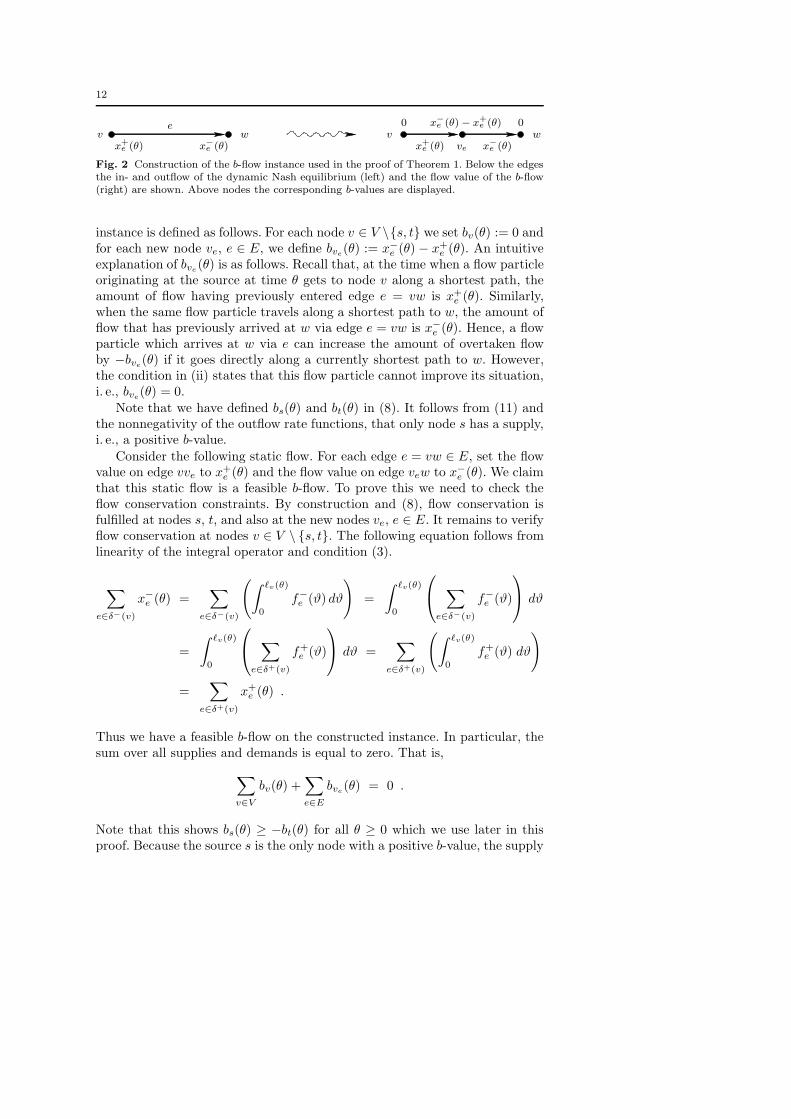
Fig. 2 Construction of the b-flow instance used in the proof of Theorem 1. Below the edgesthe in- and outflow of the dynamic Nash equilibrium (left) and the flow value of the b-flow(right) are shown. Above nodes the corresponding b-values are displayed.

instance is defined as follows. For each node v ∈ V \s, t we set bv(θ) := 0 andfor each new node ve, e ∈ E, we define bve

(θ) := x−e (θ) − x+

e (θ). An intuitiveexplanation of bve

(θ) is as follows. Recall that, at the time when a flow particleoriginating at the source at time θ gets to node v along a shortest path, theamount of flow having previously entered edge e = vw is x+

e (θ). Similarly,when the same flow particle travels along a shortest path to w, the amount offlow that has previously arrived at w via edge e = vw is x−

e (θ). Hence, a flowparticle which arrives at w via e can increase the amount of overtaken flowby −bve

(θ) if it goes directly along a currently shortest path to w. However,the condition in (ii) states that this flow particle cannot improve its situation,i. e., bve

(θ) = 0.Note that we have defined bs(θ) and bt(θ) in (8). It follows from (11) and

the nonnegativity of the outflow rate functions, that only node s has a supply,i. e., a positive b-value.

Consider the following static flow. For each edge e = vw ∈ E, set the flowvalue on edge vve to x+

e (θ) and the flow value on edge vew to x−e (θ). We claim

that this static flow is a feasible b-flow. To prove this we need to check theflow conservation constraints. By construction and (8), flow conservation isfulfilled at nodes s, t, and also at the new nodes ve, e ∈ E. It remains to verifyflow conservation at nodes v ∈ V \ s, t. The following equation follows fromlinearity of the integral operator and condition (3).

∑

e∈δ−(v)

x−e (θ) =

∑

e∈δ−(v)

(∫ ℓv(θ)

0

f−e (ϑ) dϑ

)=

∫ ℓv(θ)

0

∑

e∈δ−(v)

f−e (ϑ)

dϑ

=

∫ ℓv(θ)

0

∑

e∈δ+(v)

f+e (ϑ)

dϑ =

∑

e∈δ+(v)

(∫ ℓv(θ)

0

f+e (ϑ) dϑ

)

=∑

e∈δ+(v)

x+e (θ) .

Thus we have a feasible b-flow on the constructed instance. In particular, thesum over all supplies and demands is equal to zero. That is,

∑

v∈V

bv(θ) +∑

e∈E

bve(θ) = 0 .

Note that this shows bs(θ) ≥ −bt(θ) for all θ ≥ 0 which we use later in thisproof. Because the source s is the only node with a positive b-value, the supply

13

of s is equal to the demand of t if and only if the b-values of all other nodesare 0.

This proves the equivalence of (ii) and (iii). It remains to prove that (iv)is equivalent to the other statements.

(i)⇒(iv): The cost ℓP (θ) of a shortest s-t-path P at time θ (see Defini-tion 1) is equal to the label ℓt(θ) of t at time θ. This is due to the fact, that thedeterministic queuing model satisfies the FIFO condition on each edge. There-fore ℓt(θ) cannot be influenced by flow particles originating at the source aftertime θ. Thus, a flow over time which sends flow only along currently shortestpaths is a Nash flow over time.

(iv)⇒(iii): Assume that (iii) is violated, i. e., there exist a point in time θsuch that bs(θ) 6= −bt(θ). As mentioned above, this implies bs(θ) > −bt(θ).Hence, there exists flow of value bs(θ)+bt(θ) which originates at s until time θbut arrives at t strictly later than ℓt(θ). Since ℓt is monotonically increasing,this flow is not routed along paths with minimum latency, thus yielding acontradiction to (iv). ⊓⊔

Note that, whenever one of the four statements in Theorem 1 holds, then x+

and x− coincide. In this case, for all θ ≥ 0, setting xe(θ) := x+e (θ) for

each e ∈ E, yields a static s-t-flow x(θ) of value bs(θ). In the following, for aflow over time satisfying the universal FIFO condition, we refer to (xe(θ))e∈E

as the underlying static flow at time θ. This flow will be studied in more detailin the next section.

4 A special class of static flows

In this section we study the underlying static flows of a Nash flow over time.It turns out that these static flows have a special structure that can be used tocharacterize, compute, and analyze Nash flows over time. Further, the networkon which these flows are considered is a special subnetwork of the originalnetwork.

Definition 5 (Current Shortest Paths Network) Consider a flow overtime on a network (G, u, s, t, τ, d). For θ ≥ 0, the current shortest paths net-work Gθ is the subnetwork induced by the edges occurring in a currentlyshortest path, i. e., edges e = vw with ℓv(θ) + τe + qe(ℓv(θ)) = ℓw(θ).

Note, that every node v is contained in any current shortest path networksince we assume that every node is reachable from s. But in general there areedges which are not contained in a current shortest path network.

Definition 6 (Thin Flow with Resetting) Let (G, u, s, t, d) be a staticnetwork and E1 ⊆ E(G) a subset of edges. A static flow x′ with flow value F

14

s t

v

w

2 2

1 1

1

1 1

1

1

2 2

1 1

0 1 43

43

1

83

53

13

43

1

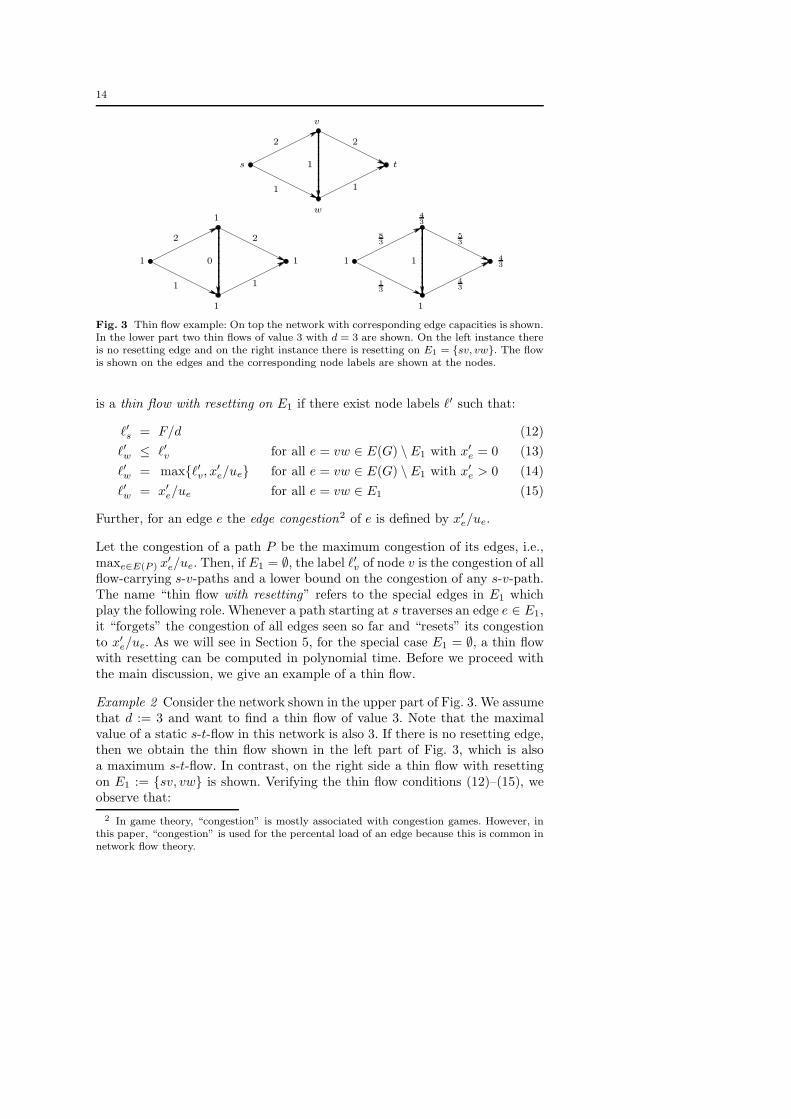
Fig. 3 Thin flow example: On top the network with corresponding edge capacities is shown.In the lower part two thin flows of value 3 with d = 3 are shown. On the left instance thereis no resetting edge and on the right instance there is resetting on E1 = sv, vw. The flowis shown on the edges and the corresponding node labels are shown at the nodes.

is a thin flow with resetting on E1 if there exist node labels ℓ′ such that:

ℓ′s = F/d (12)

ℓ′w ≤ ℓ′v for all e = vw ∈ E(G) \ E1 with x′e = 0 (13)

ℓ′w = maxℓ′v, x′e/ue for all e = vw ∈ E(G) \ E1 with x′

e > 0 (14)

ℓ′w = x′e/ue for all e = vw ∈ E1 (15)

Further, for an edge e the edge congestion2 of e is defined by x′e/ue.

Let the congestion of a path P be the maximum congestion of its edges, i.e.,maxe∈E(P ) x′

e/ue. Then, if E1 = ∅, the label ℓ′v of node v is the congestion of allflow-carrying s-v-paths and a lower bound on the congestion of any s-v-path.The name “thin flow with resetting” refers to the special edges in E1 whichplay the following role. Whenever a path starting at s traverses an edge e ∈ E1,it “forgets” the congestion of all edges seen so far and “resets” its congestionto x′

e/ue. As we will see in Section 5, for the special case E1 = ∅, a thin flowwith resetting can be computed in polynomial time. Before we proceed withthe main discussion, we give an example of a thin flow.

Example 2 Consider the network shown in the upper part of Fig. 3. We assumethat d := 3 and want to find a thin flow of value 3. Note that the maximalvalue of a static s-t-flow in this network is also 3. If there is no resetting edge,then we obtain the thin flow shown in the left part of Fig. 3, which is alsoa maximum s-t-flow. In contrast, on the right side a thin flow with resettingon E1 := sv, vw is shown. Verifying the thin flow conditions (12)–(15), weobserve that:

2 In game theory, “congestion” is mostly associated with congestion games. However, inthis paper, “congestion” is used for the percental load of an edge because this is common innetwork flow theory.

15

– the label of s satisfies (12),– the edges sw and wt satisfy (14), where the maximum is attained by the

congestion of the particular edge.– the edge vt satisfies (14), where the maximum is attained by the label of v.– the resetting edges sv and vw satisfy (15).

Also note that assuming there is no resetting edge, the right flow is not a thinflow without resetting, since vw does not satisfy (14). In fact, both thin flowsare unique on their particular instance.

Next we show that, for a Nash flow over time, the derivatives of the labelfunctions and of the underlying static flow define a thin flow with resetting.The following theorem is only applicable if the derivatives of the label andthe underlying static flow functions exist. However, both the label functionsand the underlying static flow functions are monotonically increasing implyingthat both families of functions are differentiable almost everywhere.

Theorem 2 Consider a Nash flow over time on a network (G, u, s, t, τ, d) withcorresponding label functions (ℓv)v∈V , edge waiting time functions (qe)e∈E andunderlying static flow (xe)e∈E . Let θ ≥ 0 such that dxe

dθ(θ) and dℓv

dθ(θ) exist for

each e ∈ E and v ∈ V . Then, on the current shortest paths network Gθ, thederivatives (dxe

dθ(θ))e∈E(Gθ) form a thin flow of value d with resetting on the

waiting edges E1 := e ∈ E | qe(ℓv(θ)) > 0. A corresponding set of nodelabels fulfilling (12) to (15) is given by the derivatives (dℓv

dθ(θ))v∈V (Gθ).

In order to prove Theorem 2, we need the following lemma.

Lemma 2 Let f be a flow over time which sends flow only along currentlyshortest paths on a network (G, u, τ, s, t, d). Further, let e = vw ∈ E be anedge and θ ≥ 0 be a time such that there exists a nonzero waiting queue on e,i. e., qe(ℓv(θ)) > 0. Then, edge e is contained in a shortest path at time θ.

Proof We have to show that ℓv(θ)+τe+qe(ℓv(θ)) = ℓw(θ). Let θ1 be the earliesttime such that no measurable amount of flow is assigned to e within the timeinterval [ℓv(θ1), ℓv(θ)). Then, for each ǫ > 0, there exists a θǫ ∈ [θ1 − ǫ, θ1)such that flow is assigned to e at time ℓv(θǫ). This means that e is containedin a shortest path at time θǫ. Let ǫ tend to zero. Since the label and edgewaiting time functions are continuous we get ℓv(θ1)+ τe + qe(ℓv(θ1)) = ℓw(θ1).But this implies ℓv(θ) + τe + qe(ℓv(θ)) = ℓw(θ1) because of Proposition 1(iii).Further, we know that the label functions are increasing which completes theproof because of the definition of the label functions in (6). ⊓⊔

Proof (of Theorem 2) We have to show that (dxe

dθ(θ))e∈E(Gθ) and the labels

(dℓv

dθ(θ))v∈V (Gθ) satisfy the thin flow with resetting conditions (12) to (15) with

respect to the edge set E1 := e ∈ E | qe(θ) > 0.Condition (12) for the label of s is implied by equation (6) defining the

label ℓs. In order to prove the other conditions, we distinguish three casesand show that conditions (13) to (15) are satisfied in every case. Consider an

16

edge e = vw ∈ E(Gθ) which is contained in a currently shortest s-t-path attime θ ≥ 0.

Case 1: Edge e fits this case if there exists an ǫ > 0 such that, for allθ′ ∈ (θ, θ + ǫ], we have qe(ℓv(θ′)) > 0. This means a waiting queue is built oroccurs which does not decrease to zero over a small time interval. In particular,if e ∈ E1, then e belongs to this case. Because e is used up to its capacity inthis case, we get:

xe(θ + ǫ) − xe(θ) =

∫ ℓw(θ+ǫ)

ℓw(θ)

f−e (ϑ) dϑ = ue ·

(ℓw(θ + ǫ) − ℓw(θ)

).

Dividing both sides of the last equation by ǫ and letting ǫ tend to zero, weobtain

dℓw

dθ(θ) =

dxe

dθ(θ) ·

1

ue

.

Therefore condition (15) is satisfied in this case. Further, condition (13) is alsosatisfied because the label functions are monotonically increasing. In orderto show that condition (14) is also valid in this case, we have to show thatdℓv

dθ(θ) ≤ dℓw

dθ(θ) if there is no waiting queue on e, i. e., ℓv(θ) + τe = ℓw(θ).

Because we know that e is contained in a shortest path for all times in (θ, θ+ǫ],we can conclude that

ℓv(θ + ǫ) − ℓv(θ) = ℓw(θ + ǫ) − ℓw(θ) − qe(ℓv(θ + ǫ)) ≤ ℓw(θ + ǫ) − ℓw(θ) .

This yields the desired result if we divide both sides by ǫ and let ǫ tend tozero.

Case 2: Here we consider the case that there exists an ǫ such that, for allθ′ ∈ (θ, θ + ǫ], we have ℓv(θ

′) + τe + qe(ℓv(θ′)) > ℓw(θ′). That is, edge e is not

contained in a shortest path for all times in (θ, θ + ǫ]. Note that this case isdisjoint from Case 1 because of Lemma 2. Further, we know that qe(ℓv(θ′)) = 0for all θ′ ∈ [θ, θ+ǫ]. Therefore, it holds that ℓv(θ+ǫ)−ℓv(θ) ≥ ℓw(θ+ǫ)−ℓw(θ).Moreover, we know that no flow is assigned to e during the time interval(ℓv(θ), ℓv(θ + ǫ)], i. e., xe(θ + ǫ) − xe(θ) = 0. Thus, dividing both sides of thelast inequality and of the last equation by ǫ and letting ǫ tend to zero, yields

dℓw

dθ(θ) ≤

dℓv

dθ(θ) and

dxe

dθ(θ) = 0 .

Thus, condition (13) is satisfied and the two other conditions are not relevantin this case.

Case 3: We first consider the complement of Case 2. This means, forevery ǫ > 0, there exists an θǫ ∈ (θ, θ + ǫ] such that ℓv(θǫ) + τe + qe(ℓv(θǫ)) =ℓw(θǫ). Because we can use the fact that we need not consider situations whichfall in Case 1, we can assume further that there exists a θ′ ∈ (θ, θǫ] suchthat qe(ℓv(θ

′)) = 0. Let θ′ǫ ∈ (θ, θǫ] be the supremum over these θ′. Becausethe edge waiting time functions are continuous, θ′ǫ is in fact a maximum,implying qe(ℓv(θ

′ǫ)) = 0. Further, we know that between the times θ′ǫ and θǫ

17

there is always a nonzero waiting queue. Lemma 2 and the continuity of thelabel functions show that e occurs also in a shortest path at time θ′ǫ, that is,ℓv(θ

′ǫ) + τe = ℓw(θ′ǫ). But this leads to ℓv(θ

′ǫ) − ℓv(θ) = ℓw(θ′ǫ) − ℓw(θ). If we

divide both sides of the last equation by θ′ǫ − θ and let ǫ tend to zero, we get

dℓw

dθ(θ) =

dℓv

dθ(θ) .

Therefore, condition (13) is satisfied. Because condition (15) does not applyin this case, we only show that condition (14) is valid. For this, we show thatdxe

dθ(θ) · 1

ue≤ dℓw

dθ(θ). From condition (1) in the flow over time model we get

xe(θ + ǫ) − xe(θ) =

∫ ℓw(θ+ǫ)

ℓw(θ)

f−e (ϑ) dϑ ≤

(ℓw(θ + ǫ) − ℓw(θ)

)· ue .

If we divide both sides by ǫ and let ǫ tend to zero, we get the desired result.This completes the proof. ⊓⊔

The reverse direction of Theorem 2 also holds. If, for all times θ, the deriva-tives of the underlying static flow functions and the label functions of a flowover time are thin flows with resetting in the current shortest paths network,then the flow over time is in fact a Nash flow over time. The following The-orem 3 is not the direct conversion of Theorem 2 but rather a corollary ofthe reverse direction. It shows that a Nash flow over time can be seen as theconcatenation of thin flows with resetting, which are static flows.

The scenario is the following. We assume that we already have a flowover time f := (f+, f−) showing the selfish routing behavior of flow particlesoriginating at s until a certain time θ. That is, f is a Nash flow for the “supply”function

d(ϑ) =

d for ϑ < θ

0 for ϑ ≥ θ.

Note that this does not really fit the model with a constant supply rate.But since the deterministic queuing model satisfies universal FIFO, all of theprevious results carry over to this case. We call such a flow f a restricted Nashflow over time on [0, θ).

In order to extend f , we compute a thin flow x′ on the current shortestpath network (Gθ, s, t, u) of value d with resetting on the waiting edges givenby E1 := e ∈ E | qe(ℓ(v)) > 0. Let ℓ′ be the corresponding node labels ofthe thin flow x′. For an α > 0, we extend the node label functions ℓ of f :

ℓv(ϑ) := ℓv(θ) + (ϑ − θ) · ℓ′v for all v ∈ V and ϑ ∈ [θ, θ + α) . (16)

Then, we also extend the flow rate functions:

f+e (ϑ) :=

x′e

ℓ′vfor all e = vw ∈ E and ϑ ∈ [ℓv(θ), ℓv(θ + α)) , (17)

f−e (ϑ) :=

x′e

ℓ′wfor all e = vw ∈ E and ϑ ∈ [ℓw(θ), ℓw(θ + α)) . (18)

18

The result is called an α-extension of f .We want to show that an α-extension is a feasible Nash flow over time. For

this we have to choose α appropriately such that:

ℓw(θ) − ℓv(θ) + α(ℓ′w − ℓ′v) ≥ τe for all e ∈ E1 , (19)

ℓw(θ) − ℓv(θ) + α(ℓ′w − ℓ′v) ≤ τe for all e ∈ E \ E(Gθ) . (20)

It is essential to show that α can be chosen strictly positive. In order to provethis, first observe that ℓw(θ) − ℓv(θ) − τe = qe(ℓv(θ)) > 0 for all edges e ∈ E1.Hence, there exists an α1 > 0 such that (19) is satisfied for all α ≤ α1. Thesecond condition (20) refers to edges e = vw which are not contained in theshortest path network at time θ, i. e., ℓw(θ) < ℓv(θ) + τe. Thus, there existsan α2 > 0 such that the second condition is satisfied for all α ≤ α2. This showsthe existence of an α > 0 satisfying both conditions simultaneously.

In order to extend a restricted flow as far as possible, α must be chosen aslarge as possible. That is, α > 0 can be interpreted as the largest number suchthat no waiting queue decreases to 0 and no new edge is added to the currentshortest path network. In particular, all edges satisfying (19) with equality areremoved from the set of resetting edges E1, and all edges satisfying (20) withequality are added to the current shortest path network at time θ + α.

If we insert the extension of the node labels in the two conditions on α, weobtain the following for all ϑ ∈ [θ, θ + α) (using (14) in addition):

ℓw(ϑ) ≥ ℓv(ϑ) + τe for all e = vw ∈ E(Gθ) with x′e > 0 ,

ℓw(ϑ) ≤ ℓv(ϑ) + τe for all e = vw ∈ E \ E(Gθ) .

This is used in the proof of the following theorem.

Theorem 3 Let f be a restricted Nash flow over time on [0, θ) and let α > 0be a positive real number satisfying (19) and (20). Then, the α-extension of fis a restricted Nash flow over time on [0, θ + α).

Proof We show first that the α-extension of f is a feasible flow over time.Afterwards we show that the α-extension of f is also a Nash flow over time.

In order to show that the α-extension is a feasible flow over time, we haveto show the validity of (1), (2), and (3). Since f is a restricted Nash flowover time on [0, θ), it is enough to check these conditions from time ℓv(θ) on.Further, conditions (1) and (2) are obviously satisfied if x′

e = 0. Let e = vw bean edge with x′

e > 0 and ϑ ∈ [θ, θ + α) be a point in time. From Definition 6we know that ℓ′w ≥ x′

e/ue if x′e > 0, and hence

f−e (ℓv(ϑ)) =

x′e

ℓ′w≤ ue .

This proves (1). In order to prove (2), we observe that

F+e (ℓv(ϑ)) = F+

e (ℓv(θ)) + (ℓv(ϑ) − ℓv(θ)) ·x′

e

ℓ′v

19

and

F−e (ℓw(ϑ)) = F−

e (ℓw(θ)) + (ℓw(ϑ) − ℓw(θ)) ·x′

e

ℓ′w.

Since f is a restricted Nash flow on [0, θ), we know that F+e (ℓv(θ)) = F−

e (ℓw(θ)).In addition, we obtain from the definition of the α-extension that

(ℓv(ϑ) − ℓv(θ)) ·x′

e

ℓ′v= (ϑ − θ) · ℓ′v ·

x′e

ℓ′v

= (ϑ − θ) · ℓ′w ·x′

e

ℓ′w= (ℓw(ϑ) − ℓw(θ)) ·

x′e

ℓ′w.

This yields F+e (ℓv(ϑ)) = F−

e (ℓw(ϑ)) and proves (2) since ℓw(ϑ) ≥ ℓv(ϑ) + τe ifx′

e > 0 (which is implied by (19)). Finally, (3) is satisfied because x′ satisfiesthe static flow conservation constraints which implies

∑

e∈δ−(v)

f−e (ℓ(ϑ)) =

∑

e∈δ−(v)

x′

ℓ′v=

∑

e∈δ+(v)

x′

ℓ′v=

∑

e∈δ+(v)

f+e (ℓ(ϑ)) .

Hence, the α-extension of f is a feasible flow over time.It remains to show that the α-extension is also a Nash flow over time. For

this, we show that the extended label functions coincide with label functionsdefined by (6) and we show that condition (ii) of Theorem 1 is satisfied. Ifx′

e > 0, Condition (ii) of Theorem 1 is already proved since, as shown above,we know that

x+e (ϑ) := F+

e (ℓv(ϑ)) = F−e (ℓw(ϑ)) =: x−

e (ϑ) .

For all other edges, condition (ii) of Theorem 1 is still valid because f is arestricted Nash flow.

Since ℓ′s = 1 because of (12), the first condition of (6) regarding the labelof s is obviously satisfied. If x′

e > 0, the equations F+e (ℓv(ϑ)) = F−

e (ℓw(ϑ))imply ℓv(ϑ)+τe+qe(ℓv(ϑ)) = ℓw(ϑ). Next, we consider edges e = vw containedin the shortest path network at time θ with x′

e = 0. It is not hard to see thatfor these edges we have qe(ℓv(θ)) = 0. But then condition (13) implies thatℓv(ϑ)+ τe ≥ ℓw(ϑ) for ϑ ≥ θ. Hence, it remains to show ℓv(ϑ)+ τe ≥ ℓw(ϑ) forall ϑ ≥ θ for edges which are not in the shortest path network at time θ. Butthis follows directly from the definition of α.

We have thus shown that the α-extension of f is a restricted Nash flowover time on [0, θ + α). ⊓⊔

Theorem 3 shows that a restricted Nash flow over time is extendable by aparticular thin flow with resetting. Hence, a dynamic Nash flow can be seen asthe concatenation of such static flows. In what follows, we exemplarily showhow the α-extension can be used in order to construct a Nash flow over time.

20

st

v

w

(2, 1) (2, 5)

(1, 6) (1, 1)

(1, 1)3

Fig. 4 The network used in Example 3 for which we construct a Nash flow over time. Onthe incoming edge of the source s the supply rate is shown. For all other edges e, the pair(ue, τe) denotes the capacity ue and the free flow transit time τe.

13

32

3

3

3

33

Fig. 5 The thin flow on the zigzag path.

Example 3 Consider the network (G, u, τ, s, t, d) shown in Fig. 4. In order toconstruct a Nash flow over time, we first start at time 0 with the zero flowand compute an α-extension for some suitable α > 0. Recalling Theorem 3,the α-extension results in a restricted Nash flow over time f . Next, we computeagain an α-extension for f implying that f remains a restricted Nash flow, butnow on a longer time interval. In the following we do not evaluate the in- andoutflow rate function explicitly since we want to focus on the intersting part ofthis Nash flow computation. Note, however, that they can be easily computedusing (17) and (18).

Before computing an α-extension for the zero flow, we have to identifythe current shortest path network G0 and need to evaluate the node labelfunctions at time 0. It is quite obvious that G0 is given by the zigzag pathsvwt and that (ℓs(0), ℓv(0), ℓw(0), ℓt(0)) = (0, 1, 2, 3). Since no waiting queueexists at this initial state, we have to find a thin flow x′ of value d = 3 on(G0, u, s, t) without resetting, i. e., E1 = ∅. Fig. 5 shows x′ together with thecorresponding node labels ℓ′. Next, we have to choose an α satisfying (19)and (20). Since there is no waiting edge, we have to verify condition (20) forthe edges sw and vt, which are not contained in G0. Hence, α has to satisfy:

2 + 2α = ℓw(0) − ℓs(0) + α(ℓ′w − ℓ′s) ≤ τsw = 6 ,

2 +3

2α = ℓt(0) − ℓv(0) + α(ℓ′t − ℓ′v) ≤ τvt = 5 .

Of course, we choose α as big as possible. Therefore we set α := 2. Thus theα-extension results in a restricted Nash flow on the time interval [0, 2).

In order to extend this flow further, first note that both inequalities aresatisfied with equality and hence, at time 2 both edges, sw and vt, enter thecurrent shortest path network, i. e., G2 = G. Using (16), the label functions at

21

time 2 are (ℓs(2), ℓv(2), ℓw(2), ℓt(2)) = (2, 4, 8, 9). This shows that on sv andvw the experienced travel time is greater than the free flow transit time. Thus,there must be a waiting queue on sv and vw at this state. Recalling Example 2,the thin flow x′ on (G2, u, s, t) with resetting on E1 = sv, vw is shown inthe right part of Fig. 3, and the corresponding node labels are (ℓ′s, ℓ

′v, ℓ

′w, ℓ′t) =

(1, 43 , 1, 4

3 ). Like in the first stage, we have to choose an α satisfying (19) and(20). But since G2 = G, we now have to verify condition (19) for the edges svand vw. Hence, α needs to satisfy

2 +1

3α = ℓv(2) − ℓs(2) + α(ℓ′v − ℓ′s) ≥ τsv = 1 ,

4 −1

3α = ℓw(2) − ℓv(2) + α(ℓ′w − ℓ′v) ≥ τvw = 1 .

Note that the first inequality is valid for all nonnegative α. Hence, we set α suchthat the second inequality is satisfied with equality, i. e., α := 9. Thus, the α-extension is a restricted Nash flow over time up to time 11. Using (16), the labelfunctions at time 11 are (ℓs(11), ℓv(11), ℓw(11), ℓt(11)) = (11, 16, 17, 21). Thisshows that the flow particle which start traversing the network at time 11 hasto wait on sv and wt. On the other hand, the waiting queue on vw disappearscompletely within the time interval [2, 11).

In the last iteration, we have to consider the current shortest path net-work G11 at time 11, which is again equal to G. Next we have to compute athin flow x′ on (G11, u, s, t) with resetting on sv and wt. We can easily see,that x′ is equal to the maximum s-t-flow, i. e., x′

e = ue for all edges e 6= vw,and the corresponding node labels are all equal to 1. Without going into de-tails, we note that we can set α to +∞ without violating (19) and (20). Hence,this α-extension results in a Nash flow over time on the network shown in Fig-ure 4 (defined for all nonnegative points in time). Since all node labels of x′

are equal to 1, the experienced travel time of each edge remains constant fromtime 11 on. In particular, the lengths of the waiting queues on sv and wt donot vary over time.

5 Nash flows over time and the price of anarchy

The characterization of Nash flows over time via thin flows with resettingenables us to completely analyze shortest paths networks where every s-t-pathhas the same total free flow transit time. An important subclass of shortestpaths networks are networks where the free flow travel times of each edgeis zero. We study the price of anarchy which, in general, is the worst caseratio of the cost of a Nash equilibrium and the cost of a system optimum.In the context of routing games over time, we define the price of anarchy ofan instance as the worst case ratio over all points in time θ regarding thefollowing objective:3 For given θ, maximize the amount of flow arriving atthe sink until time θ. In particular, according to this definition, earliest arrival

3 This objective is well motivated if we think of, e. g., modeling an evacuation situation.

22

flows that maximize the amount of flow at the sink simultaneously for all pointsin time, are system optima. In addition, an earliest arrival flow optimizes alsothe following objective functions simultaneously for all times θ and for eachdemand value F , respectively: the average inflow rate in t until time θ, thetotal time needed to send a demand of value F to t, the average arrival timefor a demand of value F (see, e. g., [23]). Hence, the following theorem showsthat, on shortest paths networks, the price of anarchy is 1 for each of theseobjective functions.

Theorem 4 For shortest paths networks, each Nash flow over time is an ear-liest arrival flow and thus a system optimum. Moreover, a Nash flow over timecan be computed in polynomial time.

For proving this, we analyze thin flows without resetting. Therefore we firstdiscuss the results related to this part before we give a proof of Theorem 4.The following is an equivalent definition of thin flows without resetting, i. e.,thin flows with resetting on E1 = ∅.

Definition 7 For a network (G, u, s, t), a static s-t-flow x′ ∈ RE(G) is calledthin flow if, for each node v, every flow carrying s-v-path has the same conges-tion ℓ′v and every s-v-path has congestion at least ℓ′v. If, in addition, a supply d

is given, we initialize ℓ′s := |x′|d

where |x′| is the flow value of x′.

In order to study thin flows, we can restrict to instances with infinite supplyrate d, i. e., ℓ′s = 0. This is due to the fact that we can model a finite supplysimply by adding a dummy source s0 and an edge s0s with capacity d to thenetwork. Then, of course, a thin flow on the new instance corresponds to athin flow on the original instance and vice versa. Further, the definition ofthin flows is directly generalizable to b-flow instances (G, u, b) where only onenode s has a positive supply, i. e., bs > 0 and bv ≤ 0 for all v ∈ V \ s. Nextwe prove some properties of thin flows. We define an edge label ℓ′e for each

edge e = vw ∈ E by ℓ′e := maxℓ′v,x′

e

ue.

Lemma 3 Let x′ be a thin b-flow on a network (G, u, b) where only one node shas a positive supply. Then, the maximum label ℓ′max of any edge is equal to thecongestion q∗ of a sparsest cut in (G, u, b), i. e., a node set X ⊂ V maximizing

b(X)u(δ+(X)) , where u(δ+(X)) :=

∑e∈δ+(X) ue.

Proof The relation ℓ′max ≥ q∗ is obvious because at least one edge in a sparsestcut must have congestion at least q∗ in any b-flow. Thus, we have to showthat ℓ′max ≤ q∗. Consider the cut s ∈ X V defined by the set of nodesX := v ∈ V | ℓ′v < ℓ′max. Since the labels of the nodes in X are strictlysmaller than the labels of the nodes not in X , there is no flow on any edgein δ−(X). Further, the congestion of any edge in δ+(X) is at least ℓ′max. Thisleads to

ℓ′max ≤x(δ+(X))

u(δ+(X))=

b(X)

u(δ+(X))≤ q∗ ,

because q∗ is the congestion of a sparsest cut. ⊓⊔

23

The last lemma shows that a thin s-t-flow of value equal to the maximums-t-flow value is also feasible with respect to edge capacities. The next lemmashows that thin flows are unique with respect to node labels. Moreover, thinflows without resetting can be computed in polynomial time by a sequence ofsparsest cut computations.

Lemma 4 Consider a pair of thin flows with the same s-t-flow value or thesame node balances b. Then, the node labels ℓ′v are identical. Moreover, a thinflow of given flow value can be computed in polynomial time.

Proof Consider two thin flows x′, x ∈ RE(G)+ . We prove by induction on the

number of nodes that the corresponding edge labels ℓ′, ℓ are identical. Then,this must also hold for the corresponding node labels. If there is only onenode s, nothing has to be proved. Let us thus assume that there are severalnodes. Lemma 3 shows that the maximum edge label ℓ′max is unique for x′

and x and equal to the congestion of a sparsest cut. Let δ+(X) be the sparsestcut where X ⊂ V is inclusionwise minimal. Then, the labels of the edges onand behind δ+(X) coincide for x′ and x, and are equal to ℓ′max. Further, weknow the flow values on edges contained in δ+(X), because the labels of suchedges must be defined by their congestion, i. e., x′

e = xe = ℓ′max · ue.Now we delete the node set V \X . Then, x′ and x ∈ RE(G) are thin b-flows

on the induced subgraph G[X ] according to the new node balances

b′(v) := b(v) − x′(δ+G(v) ∩ δ+(X)

)for all v ∈ X .

Since the graph G[X ] has less nodes than G, we can apply the inductionhypothesis and conclude this part of the proof.

We finally argue that we can compute a thin flow of given flow value inpolynomial time. Note that the induction above is constructive and describesan algorithm where, in each iteration, we have to compute a sparsest cut fora b-flow instance. This can be done in polynomial time. Moreover the numberof iterations is bounded by the number of nodes. Note that an algorithmfor computing a sparsest cut usually also computes a flow minimizing themaximum edge congestion. This flow is used to obtain the flow values foredges behind the sparsest cut. ⊓⊔

Next we give the proof of Theorem 4.

Proof (Proof of Theorem 4) First note that the current shortest path networkat time 0 is the entire network. Since at time 0 no waiting occurs, Theorem 3is valid for α = ∞ and shows that a thin flow x′ without resetting on theshortest path network results in a Nash flow over time f (defined for all times).Lemma 3 implies that f sends, at each point in time, the maximum possibleflow rate into t. This can be seen as follows. Let ℓ′ be the corresponding nodelabels of x′ and let F ∗ be the maximum static flow value on (G, u, s, t). Then,Lemma 3 shows that the label of t is ℓ′t = d

F∗. Hence, the definition of the flow

rate functions in an α-extension shows that the inflow rate in t is |x′|ℓ′

t

= F ∗.

24

s = vm v1 = tv2v3v4 e1 = e1

e2

e3

e4

em

e2e3em

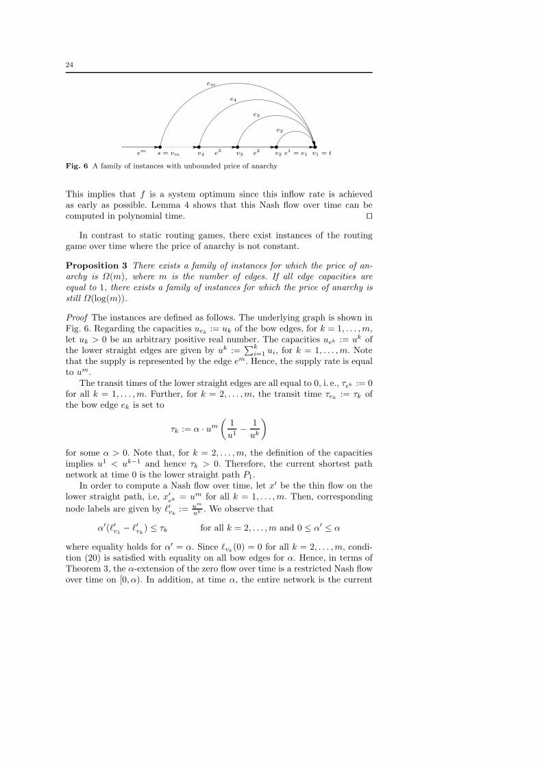
Fig. 6 A family of instances with unbounded price of anarchy

This implies that f is a system optimum since this inflow rate is achievedas early as possible. Lemma 4 shows that this Nash flow over time can becomputed in polynomial time. ⊓⊔

In contrast to static routing games, there exist instances of the routinggame over time where the price of anarchy is not constant.

Proposition 3 There exists a family of instances for which the price of an-archy is Ω(m), where m is the number of edges. If all edge capacities areequal to 1, there exists a family of instances for which the price of anarchy isstill Ω(log(m)).

Proof The instances are defined as follows. The underlying graph is shown inFig. 6. Regarding the capacities uek

:= uk of the bow edges, for k = 1, . . . , m,let uk > 0 be an arbitrary positive real number. The capacities uek := uk ofthe lower straight edges are given by uk :=

∑k

i=1 ui, for k = 1, . . . , m. Notethat the supply is represented by the edge em. Hence, the supply rate is equalto um.

The transit times of the lower straight edges are all equal to 0, i. e., τek := 0for all k = 1, . . . , m. Further, for k = 2, . . . , m, the transit time τek

:= τk ofthe bow edge ek is set to

τk := α · um

(1

u1−

1

uk

)

for some α > 0. Note that, for k = 2, . . . , m, the definition of the capacitiesimplies u1 < uk−1 and hence τk > 0. Therefore, the current shortest pathnetwork at time 0 is the lower straight path P1.

In order to compute a Nash flow over time, let x′ be the thin flow on thelower straight path, i.e, x′

ek = um for all k = 1, . . . , m. Then, corresponding

node labels are given by ℓ′vk:= um

uk . We observe that

α′(ℓ′v1− ℓ′vk

) ≤ τk for all k = 2, . . . , m and 0 ≤ α′ ≤ α

where equality holds for α′ = α. Since ℓvk(0) = 0 for all k = 2, . . . , m, condi-

tion (20) is satisfied with equality on all bow edges for α. Hence, in terms ofTheorem 3, the α-extension of the zero flow over time is a restricted Nash flowover time on [0, α). In addition, at time α, the entire network is the current

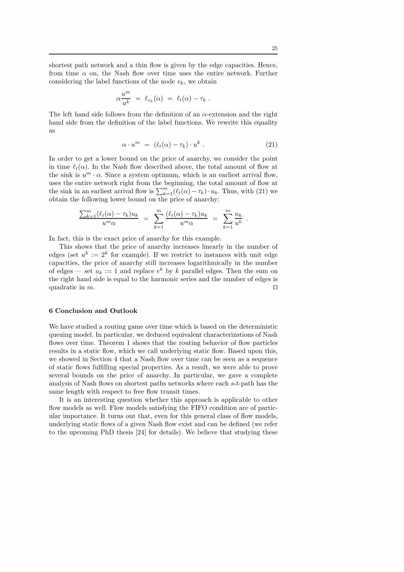
25

shortest path network and a thin flow is given by the edge capacities. Hence,from time α on, the Nash flow over time uses the entire network. Furtherconsidering the label functions of the node vk, we obtain

αum

uk= ℓvk

(α) = ℓt(α) − τk .

The left hand side follows from the definition of an α-extension and the righthand side from the definition of the label functions. We rewrite this equalityas

α · um = (ℓt(α) − τk) · uk . (21)

In order to get a lower bound on the price of anarchy, we consider the pointin time ℓt(α). In the Nash flow described above, the total amount of flow atthe sink is um · α. Since a system optimum, which is an earliest arrival flow,uses the entire network right from the beginning, the total amount of flow atthe sink in an earliest arrival flow is

∑m

k=1(ℓt(α)− τk) ·uk. Thus, with (21) weobtain the following lower bound on the price of anarchy:

∑m

k=1(ℓt(α) − τk)uk

umα=

m∑

k=1

(ℓt(α) − τk)uk

umα=

m∑

k=1

uk

uk.

In fact, this is the exact price of anarchy for this example.This shows that the price of anarchy increases linearly in the number of

edges (set uk := 2k for example). If we restrict to instances with unit edgecapacities, the price of anarchy still increases logarithmically in the numberof edges — set uk := 1 and replace ek by k parallel edges. Then the sum onthe right hand side is equal to the harmonic series and the number of edges isquadratic in m. ⊓⊔

6 Conclusion and Outlook

We have studied a routing game over time which is based on the deterministicqueuing model. In particular, we deduced equivalent characterizations of Nashflows over time. Theorem 1 shows that the routing behavior of flow particlesresults in a static flow, which we call underlying static flow. Based upon this,we showed in Section 4 that a Nash flow over time can be seen as a sequenceof static flows fulfilling special properties. As a result, we were able to proveseveral bounds on the price of anarchy. In particular, we gave a completeanalysis of Nash flows on shortest paths networks where each s-t-path has thesame length with respect to free flow transit times.

It is an interesting question whether this approach is applicable to otherflow models as well. Flow models satisfying the FIFO condition are of partic-ular importance. It turns out that, even for this general class of flow models,underlying static flows of a given Nash flow exist and can be defined (we referto the upcoming PhD thesis [24] for details). We believe that studying these

26

special flows is a promising direction for analyzing Nash flows in the corre-sponding flow model. Natural candidates for future research are flow modelswith linear load-dependent transit times (see [26]) as well as the flow modelof Daganzo (see [13]). The model of Daganzo is a generalization of the deter-ministic queuing model in which the size of the waiting queues are boundedby given constants.

Finally, we remark that the presented results remain true with tiny modi-fications if edge capacities are allowed to vary over time. This model is harderto analyze since the effective transit time of an edge is in general discontinuousif the capacity vanishes over a time interval.

Acknowledgments. The authors are much indebted to Jose Correa for inspiringdiscussions on the topic of this paper. The authors would also like to thank thereferees of [25] and the referees of this paper for numerous valuable suggestionsand comments that helped to improve the presentation of the paper.

References

1. T. Akamatsu. A dynamic traffic equilibrium assignment paradox. Transportation Re-

search B, 34(6):515–531, 2000.2. T. Akamatsu. An efficient algorithm for dynamic traffic equilibrium assignment with

queues. Transportation Science, 35(4):389–404, 2001.3. T. Akamatsu and B. Heydecker. Detecting dynamic traffic assignment capacity para-

doxes in saturated networks. Transportation Science, 37(2):123–138, 2003.4. E. Anshelevich and S. Ukkusuri. Equilibria in dynamic selfish routing. In M. Mavron-

icolas, editor, Proceedings of the 2nd International Symposium on Algorithmic Game

Theory, volume 5814 of Lecture Notes in Computer Science, pages 171–182. Springer,2009.

5. J. E. Aronson. A survey of dynamic network flows. Annals of Operations Research,20(1–4):1–66, 1989.

6. M. Balmer, M. Rieser, K. Meister, D. Charypar, N. Lefebvre, and K. Nagel. MATSim-T: Architecture and simulation times. In A. Bazzan and F. Klugl, editors, Multi-Agent

Systems for Traffic and Transportation Engineering, chapter III. Information ScienceReference, 2009.

7. M. J. Ben-Akiva, M. Bierlaire, H. N. Koutsopoulos, and R. Mishalani. Dynamit: Asimulation-based system for traffic prediction and guidance generation. In Proceedings

of the 3rd Triennial Symposium on Transportation Systems, 1998.8. D. Braess. Uber ein Paradoxon aus der Verkehrsplanung. Unternehmensforschung 12,

12:258–268, 1968. In German.9. M. Carey. Link travel times I: Properties derived from traffic-flow models. Networks

and Spatial Economics, 4(3):257–268, 2004.10. M. Carey. Link travel times II: Properties derived from traffic-flow models. Networks

and Spatial Economics, 4(4):379–402, 2004.11. H.-K. Chen. Dynamic Travel Choice Models: A Variational Inequality Approach.

Springer, 1999.12. H.-K. Chen and C.-F. Hsueh. A model and an algorithm for the dynamic user-optimal

route choice problem. Transportation Research B, 32(3):219–234, 1998.13. C. F. Daganzo. Queue spillovers in transportation networks with a route choice. Trans-

portation Science, 32(1):3–11, 1998.

14. L. K. Fleischer and E. Tardos. Efficient continuous-time dynamic network flow algo-rithms. Operations Research Letters, 23(3-5):71–80, 1998.

15. L. R. Ford and D. R. Fulkerson. Constructing maximal dynamic flows from static flows.Operations Research, 6(3):419–433, 1958.

27

16. L. R. Ford and D. R. Fulkerson. Flows in Networks. Princeton University Press, 1962.17. T. L. Friesz, D. Bernstein, T. E. Smith, R. L. Tobin, and B. W. Wie. A variational

inequality formulation of the dynamic network user equilibrium problem. Operations

Research, 41(1):179–191, 1993.18. T. L. Friesz, J. Luque, R. L. Tobin, and B. W. Wie. Dynamic network traffic assign-

ment considered as a continuous time optimal control problem. Operations Research,37(6):893–901, 1989.

19. H. W. Hamacher and S. A. Tjandra. Mathematical modelling of evacuation problems:A state of the art. In M. Schreckenberg and S. D. Sharma, editors, Pedestrian and

Evacuation Dynamics, pages 227–266. Springer, 2002.20. S. Han and B. G. Heydecker. Consistent objectives and solution of dynamic user equi-

librium models. Transportation Research B, 40(1):16–34, 2006.21. C. Hendrickson and G. Kocur. Schedule delay and departure time decisions in a deter-

ministic model. Transportation Science, 15(1):62–77, 1981.22. M. Hoefer, V. Mirrokni, H. Roglin, and S.-H. Teng. Competitive routing over time.

In S. Leonardi, editor, Proceedings of the 5th International Workshop on Internet and

Network Economics, volume 5929 of Lecture Notes in Computer Science, pages 18–29.Springer, 2009.

23. J. J. Jarvis and H. D. Ratliff. Some equivalent objectives for dynamic network flowproblems. Management Science, 28:106–108, 1982.

24. R. Koch. PhD thesis, TU Berlin. In preparation.25. R. Koch and M. Skutella. Nash equilibria and the price of anarchy for flows over

time. In M. Mavronicolas, editor, Proceedings of the 2nd International Symposium on

Algorithmic Game, volume 5814 of Lecture Notes in Computer Science, pages 323–334.Springer, 2009.

26. E. Kohler and M. Skutella. Flows over time with load-dependent transit times. SIAM

Journal on Optimization, 15:1185–1202, 2005.27. B. Korte and J. Vygen. Combinatorial Optimization: Theory and Algorithms. Springer,

4th edition, 2008.28. W. H. Lin and H. K. Lo. Are the objective and solutions of dynamic user-equilibrium

models always consistent? Transportation Research A, 34(2):137–144, 2000.29. H. S. Mahmassani and R. Herman. Dynamic user equilibrium departure time and route

choice on idealized traffic arterials. Transportation Science, 18(4):362–384, 1984.30. H. S. Mahmassani and S. Peeta. System optimal dynamic assignment for electronic

route guidance in a congested traffic network. In N. H. Gartner and G. Improta, editors,Urban Traffic Networks. Dynamic Flow Modelling and Control, pages 3–37. Springer,Berlin, 1995.

31. H. S. Mahmassani, H. A. Sbayti, and X. Zhou. DYNASMART-P Version 1.0 Users

Guide. Maryland Transportation Initiative, College Park, Maryland, 2004.32. R. Mounce. Convergence in a continuous dynamic queueing model for traffic networks.

Transportation Research B, 40(9):779–791, 2006.33. R. Mounce. Convergence to equilibrium in dynamic traffic networks when route cost is

decay monotone. Transportation Science, 41(3):409–414, 2007.

34. N. Nisan, T. Roughgarden, E. Tardos, and V. V. Vazirani. Algorithmic Game Theory.Cambridge University Press, 2007.

35. A. de Palma, M. Ben-Akiva, C. Lefevre, and N. Litinas. Stochastic equilibrium modelof peak period traffic congestion. Transportation Science, 17(4):430–453, 1983.

36. S. Peeta and A. K. Ziliaskopoulos. Foundations of dynamic traffic assignment: The past,the present and the future. Networks and Spatial Economics, 1(3–4):233–265, 2001.

37. W. B. Powell, P. Jaillet, and A. Odoni. Stochastic and dynamic networks and routing.In M. O. Ball, T. L. Magnanti, C. L. Monma, and G. L. Nemhauser, editors, Network

Routing, volume 8 of Handbooks in Operations Research and Management Science,chapter 3, pages 141–295. North-Holland, 1995.

38. B. Ran and D. E. Boyce. Modelling Dynamic Transportation Networks. Springer, 1996.39. B. Ran, D. E. Boyce, and L. J. Leblanc. A new class of instantaneous dynamic user-

optimal traffic assignment models. Operations Research, 41(1):192–202, 1993.40. B. Ran, R. W. Hall, and D. E. Boyce. A link-based variational inequality model for

dynamic departure time/route choice. Transportation Research B, 30(1):31–46, 1996.

28

41. T. Roughgarden. Selfish Routing and the Price of Anarchy. MIT Press, 2005.42. T. Roughgarden and E. Tardos. How bad is selfish routing? In Proceedings of the 41st

Annual IEEE Symposium on Foundations of Computer Science, pages 93–102, 2000.43. M. Skutella. An introduction to network flows over time. In W. Cook, L. Lovasz, and

J. Vygen, editors, Research Trends in Combinatorial Optimization, chapter 21, pages451–482. Springer, 2009.

44. M. J. Smith. The existence of a time-dependent equilibrium distribution of arrivals ata single bottleneck. Transportation Science, 18(4):385–394, 1984.

45. M. J. Smith. A new dynamic traffic model and the existence and calculation of dy-namic user equilibria on congested capacity-constrained road networks. Transportation

Research B, 27(1):49–63, 1993.46. W. Y. Szeto and Hong K. Lo. A cell-based simultaneous route and departure time

choice model with elastic demand. Transportation Research B, 38(7):593–612, 2004.47. N. B. Taylor. The CONTRAM dynamic traffic assignment model. Networks and Spatial

Economics, 3(3):297–322, 2003.48. W. S. Vickrey. Congestion theory and transport investment. The American Economic

Review, 59(2):251–260, 1969.49. J. H. Wu, Y. Chen, and M. Florian. The continuous dynamic network loading problem:

a mathematical formulation and solution method. Transportation Research Part B:

Methodological, 32(3):173–187, 1998.50. Y. W. Xu, J. H. Wu, M. Florian, P. Marcotte, and D. L. Zhu. Advances in the continuous

dynamic network loading problem. Transportation Science, 33(4):341–353, 1999.51. S. Yagar. Dynamic traffic assignment by individual path minimization and queuing.

Transportation Research, 5(3):179–196, 1971.