nathaniel e. helwig - school of statisticsusers.stat.umn.edu/~helwig/notes/mvmean-notes.pdf · t2...

Inferences about Multivariate Means

Nathaniel E. Helwig

Assistant Professor of Psychology and StatisticsUniversity of Minnesota (Twin Cities)

Updated 16-Jan-2017

Nathaniel E. Helwig (U of Minnesota) Inferences about Multivariate Means Updated 16-Jan-2017 : Slide 1

Copyright

Copyright c© 2017 by Nathaniel E. Helwig


Outline of Notes

1) Single Mean VectorIntroductionHotelling’s T 2

Likelihood Ratio TestsConfidence RegionsSimultaneous T 2 CIsBonferroni’s MethodLarge Sample InferencePrediction Regions

2) Multiple Mean VectorsIntroductionPaired ComparisonsRepeated MeasuresTwo PopulationsOne-Way MANOVASimultaneous CIsEqual Cov Matrix TestTwo-Way MANOVA


Inferences about a Single Mean Vector

Inferences about aSingle Mean Vector


Inferences about a Single Mean Vector Introduction

Univariate Reminder: Student’s One-Sample t Test

Let (x1, . . . , xn) denote a sample of iid observations sampled from anormal distribution with mean µ and variance σ2, i.e., xi

iid∼ N(µ, σ2).

Suppose σ2 is unknown, and we want to test the hypotheses

H0 : µ = µ0 versus H1 : µ 6= µ0

where µ0 is some known value specified by the null hypothesis.

We use Student’s t test, where the t test statistic is given by

t =x̄ − µ0

s/√

n

where x̄ = 1n∑n

i=1 xi and s2 = 1n−1

∑ni=1(xi − x̄)2.



Univariate Reminder: Student’s t Test (continued)

Under H0, the t test statistic follows a Student’s t distribution withdegrees of freedom ν = n − 1.

We reject H0 if |t | is large relative to what we would expectSame as rejecting H0 if t2 is larger than we expect

We can rewrite the (squared) t test statistic as

t2 = n(x̄ − µ0)(s2)−1(x̄ − µ0)

which emphasizes the quadratic form of the t test statistic.t2 gets larger as (x̄ − µ0) gets larger (for fixed s2 and n)t2 gets larger as s2 gets smaller (for fixed x̄ − µ0 and n)t2 get larger as n gets larger (for fixed x̄ − µ0 and s2)



Multivariate Extensions of Student’s t Test

Now suppose that xiiid∼ N(µ,Σ) where

xi = (xi1, . . . , xip)′ is the i-th observation’s p × 1 vectorµ = (µ1, . . . , µp)′ is the p × 1 mean vectorΣ = {σjk} is the p × p covariance matrix

Suppose Σ is unknown, and we want to test the hypotheses

H0 : µ = µ0 versus H1 : µ 6= µ0

where µ0 is some known vector specified by the null hypothesis.


Inferences about a Single Mean Vector Hotelling’s T 2

Hotelling’s T 2 Test Statistic

Hotellings T 2 is multivariate extension of (squared) t test statistic

T 2 = n(x̄− µ0)′S−1(x̄− µ0)

wherex̄ = 1

n∑n

i=1 xi is the sample mean vector

S = 1n−1

∑ni=1(xi − x̄)(xi − x̄)′ is the sample covariance matrix

1n S is the sample covariance matrix of x̄

Letting X = {xij} denote the n × p data matrix, we could write

x̄ = 1n∑n

i=1 xi = n−1X′1n

S = 1n−1

∑ni=1(xi − x̄)(xi − x̄)′ = 1

n−1X′cXc

Xc = CX with C = In − 1n 1n1′n denoting a centering matrix



Inferences using Hotelling’s T 2

Under H0, Hotelling’s T 2 follows a scaled F distribution

T 2 ∼ (n − 1)p(n − p)

Fp,n−p

where Fp,n−p denotes an F distribution with p numerator degrees offreedom and n − p denominator degrees of freedom.

This implies that α = P(T 2 > [p(n − 1)/(n − p)]Fp,n−p(α))

Fp,n−p(α) denotes upper (100α)th percentile of Fp,n−p distribution

We reject the null hypothesis if T 2 is too large, i.e., if

T 2 >(n − 1)p(n − p)

Fp,n−p(α)

where α is the significance level of the test.Nathaniel E. Helwig (U of Minnesota) Inferences about Multivariate Means Updated 16-Jan-2017 : Slide 9


Comparing Student’s t2 and Hotelling’s T 2

Student’s t2 and Hotelling’s T 2 have a similar form

T 2p,n−1 =

√n(x̄− µ0)′[S]−1√n(x̄− µ0)

= (MVN vector)′(

Wishart matrixdf

)−1

(MVN vector)

t2n−1 =

√n(x̄ − µ0)[s2]−1√n(x̄ − µ0)

= (UVN variable)

(scaled χ2 variable

df

)−1

(UVN variable)

where MVN (UVN) = multivariate (univariate) normal and df = n − 1.



Define Hotelling’s T 2 Test Function

T.test <- function(X, mu=0){X <- as.matrix(X)n <- nrow(X)p <- ncol(X)df2 <- n - pif(df2 < 1L) stop("Need nrow(X) > ncol(X).")if(length(mu) != p) mu <- rep(mu[1], p)xbar <- colMeans(X)S <- cov(X)T2 <- n * t(xbar - mu) %*% solve(S) %*% (xbar - mu)Fstat <- T2 / (p * (n-1) / df2)pval <- 1 - pf(Fstat, df1=p, df2=df2)data.frame(T2=as.numeric(T2), Fstat=as.numeric(Fstat),

df1=p, df2=df2, p.value=as.numeric(pval), row.names="")}



Hotelling’s T 2 Test Example in R

# get data matrix> data(mtcars)> X <- mtcars[,c("mpg","disp","hp","wt")]> xbar <- colMeans(X)

# try Hotelling T^2 function> xbar

mpg disp hp wt20.09062 230.72188 146.68750 3.21725> T.test(X)

T2 Fstat df1 df2 p.value7608.14 1717.967 4 28 0> T.test(X, mu=c(20,200,150,3))

T2 Fstat df1 df2 p.value10.78587 2.435519 4 28 0.07058328> T.test(X, mu=xbar)T2 Fstat df1 df2 p.value0 0 4 28 1



Hotelling’s T 2 Using lm Function in R

> y <- as.matrix(X)> anova(lm(y ~ 1))Analysis of Variance Table

Df Pillai approx F num Df den Df Pr(>F)(Intercept) 1 0.99594 1718 4 28 < 2.2e-16 ***Residuals 31---Signif. codes: 0 ‘***’ 0.001 ‘**’ 0.01 ‘*’ 0.05 ‘.’ 0.1 ‘ ’ 1

> y <- as.matrix(X) - matrix(c(20,200,150,3),nrow(X),ncol(X),byrow=T)> anova(lm(y ~ 1))Analysis of Variance Table

Df Pillai approx F num Df den Df Pr(>F)(Intercept) 1 0.25812 2.4355 4 28 0.07058 .Residuals 31---Signif. codes: 0 ‘***’ 0.001 ‘**’ 0.01 ‘*’ 0.05 ‘.’ 0.1 ‘ ’ 1

> y <- as.matrix(X) - matrix(xbar,nrow(X),ncol(X),byrow=T)> anova(lm(y ~ 1))Analysis of Variance Table

Df Pillai approx F num Df den Df Pr(>F)(Intercept) 1 1.8645e-31 1.3052e-30 4 28 1Residuals 31


Inferences about a Single Mean Vector Likelihood Ratio Tests

Multivariate Normal MLE Reminder

Reminder: the log-likelihood function for n independent samples froma p-variate normal distribution has the form

LL(µ,Σ|X) = −np2

log(2π)− n2

log(|Σ|)− 12

n∑i=1

(xi − µ)′Σ−1(xi − µ)

and the MLEs of the mean vector µ and covariance matrix Σ are

µ̂ =1n

n∑i=1

xi = x̄

Σ̂ =1n

n∑i=1

(xi − µ̂)(xi − µ̂)′



Multivariate Normal Maximized Likelihood Function

Plugging the MLEs of µ and Σ into the likelihood function gives

maxµ,Σ

L(µ,Σ|X) =exp(−np/2)

(2π)np/2|Σ̂|n/2

If we assume that µ = µ0 under H0, then we have that

maxΣ

L(Σ|µ0,X) =exp(−np/2)

(2π)np/2|Σ̂0|n/2

where Σ̂0 = 1n∑n

i=1(xi − µ0)(xi − µ0)′ is the MLE of Σ under H0.



Likelihood Ratio Test Statistic (and Wilks’ lambda)

Want to test H0 : µ = µ0 versus H1 : µ 6= µ0

The likelihood ratio test statistic is

Λ =maxΣ L(Σ|µ0,X)

maxµ,Σ L(µ,Σ|X)=

(|Σ̂||Σ̂0|

)n/2

and we reject H0 if the observed value of Λ is too small.

The equivalent test statistic Λ2/n = |Σ̂||Σ̂0|

is known as Wilks’ lambda.



Relationship Between T 2 and Λ

There is a simple relationship between T 2 and Λ

Λ2/n =

(1 +

T 2

n − 1

)−1

which derives from the definition of the matrix determinant.1

This implies that we can just use the T 2 distribution for Λ inference.Reject H0 for small Λ2/n ⇐⇒ large T 2

1For a proof, see p 218 of Johnson & Wichern (2007).Nathaniel E. Helwig (U of Minnesota) Inferences about Multivariate Means Updated 16-Jan-2017 : Slide 17


General Likelihood Ratio Tests

Let θ ∈ Θ denote a p × 1 vector of parameters, which takes values inthe parameter set Θ, and let θ0 ∈ Θ0 where Θ0 ⊂ Θ.

A likelihood ratio test rejects H0 : θ ∈ Θ0 in favor of H1 : θ 6∈ Θ0 if

Λ =maxθ∈Θ0 L(θ)

maxθ∈Θ L(θ)< cα

where cα is some constant and L(·) is the likelihood function.

For a large sample size n, we have that

−2 log(Λ) ≈ χ2ν−ν0

where ν and ν0 are the dimensions of Θ and Θ0.Nathaniel E. Helwig (U of Minnesota) Inferences about Multivariate Means Updated 16-Jan-2017 : Slide 18

Inferences about a Single Mean Vector Confidence Regions

Extending Confidence Intervals to Regions

A 100(1− α)% confidence interval (CI) for θ ∈ Θ is defined such that

P[Lα(x) ≤ θ ≤ Uα(x)] = 1− α

where the interval [Lα(x),Uα(x)] ⊂ Θ is a function of the data vector xand the significance level α.

A confidence region is a multivariate extension of a confidence interval.

A 100(1− α)% confidence region (CR) for θ ∈ Θ is defined such that

P[θ ∈ Rα(X)] = 1− α

where the region Rα(X) ⊂ Θ is a function of the data matrix X and thesignificance level α.Nathaniel E. Helwig (U of Minnesota) Inferences about Multivariate Means Updated 16-Jan-2017 : Slide 19


Confidence Regions for Normal Mean Vector

Before we collect n samples from a p-variate normal distribution

P[T 2 ≤ νn,pFp,n−p(α)] = 1− α

where T 2 = n(x̄− µ)′S−1(x̄− µ) and νn,p = p(n − 1)/(n − p).

The 100(1− α)% confidence region (CR) for a mean vector from ap-variate normal distribution is ellipsoid formed by all µ ∈ Rp such that

n(x̄− µ)′S−1(x̄− µ) ≤ νn,pFp,n−p(α)

where x̄ = 1n∑n

i=1 xi and S = 1n−1

∑ni=1(xi − x̄)(xi − x̄)′.



Forming Confidence Regions in R

● ● ● ●●

●●

●●

●●

●●

●●

●●

●●●●●

●●●●●●●●●

●●

●●

●●

●●

●●

●●

●●●●●●●●●

16 18 20 22 24

100

140

180

mpg

hp ***

● 0.990.950.9

●●

●●●●●●●●●

●●

●●

●●

●●

●●

●●

●●●●●●●●● ● ● ●

●●

●●

●●

●●

●●

●●

●●●●●

150 200 250 300

100

140

180

disp

hp ***

● 0.990.950.9

n <- nrow(X)p <- ncol(X)xbar <- colMeans(X)S <- cov(X)library(car)tconst <- sqrt((p/n)*((n-1)/(n-p)) * qf(0.99,p,n-p))id <- c(1,3)plot(ellipse(center=xbar[id], shape=S[id,id], radius=tconst, draw=F), xlab="mpg", ylab="hp")


Inferences about a Single Mean Vector Simultaneous T 2 Confidence Intervals

Linear Combinations of Normal Variables

Suppose that X = (X1, . . . ,Xp) ∼ N(µ,Σ) and let a = (a1, . . . ,ap) ∈ Rp

denote some linear transformation vector.

The random variable Z =∑p

j=1 ajXj = a′X has the properties

µZ = E(Z ) =

p∑j=1

ajE(Xj) = a′µ

σ2Z = Var(Z ) = a′Σa

and because Z is a linear transformation of normal variables, we know

Z ∼ N(µZ , σ2Z )

i.e., Z follows a univariate normal with mean µZ and variance σ2Z .



Linear Combinations of Multivariate Sample Means

Suppose that xiiid∼ N(µ,Σ) and zi = a′xi for i ∈ {1, . . . ,n}.

The sample mean and variance of the zi terms are

z̄ = a′x̄

s2z = a′Sa

where x̄ = 1n∑n


∑ni=1(xi − x̄)(xi − x̄)′.

Because z̄ is a linear transformation of normal variables, we know

z̄ ∼ N(µZ , σ2Z/n)

i.e., z̄ follows a univariate normal with mean µZ and variance σ2Z/n.



Confidence Intervals for Single Linear Combination

Fixing a and assuming σ2Z is unknown, the t test statistic is

t =z̄ − µZ

sz/√

n=

√n(a′x̄− a′µ)√

a′Sa

and the corresponding confidence interval has the form

z̄ − sz√n

tn−1(α/2) ≤ µZ ≤ z̄ +sz√

ntn−1(α/2)

a′x̄−√

a′Sa√n

tn−1(α/2) ≤ µZ ≤ a′x̄ +

√a′Sa√

ntn−1(α/2)

where tn−1(α/2) is the critical value that cuts off the upper (100α/2)%tail of the tn−1 distribution.



Limitation of CIs for Single Linear Combination

The confidence interval has level α separately for each CI we form.Each interval separately satisfies P[µj ∈ Rj(X)] = 1− α

For multiple CIs, the familywise significance level will exceed α.Intervals dot not satisfy P[µ1 ∈ R1(X) ∩ · · · ∩ µp ∈ Rp(X)] = 1− α

If we want to form a CI for each µj term, we need to consider someapproach that will control the familywise error rate.



Defining a Simultaneous Confidence Interval

For a fixed a, the t test statistic CI is the set of a′µ values such that

t2 =(z̄ − µZ )2

s2z/n

=n(a′x̄− a′µ)2

a′Sa≤ tn−1(α/2)

For a simultaneous CI, we want the above to hold for all choices of a.

Start by considering the maximum possible t2 that we could see

maxa

t2 = maxa

n[a′(x̄− µ)]2

a′Sa= n(x̄− µ)′S−1(x̄− µ) = T 2

which occurs when a ∝ S−1(x̄− µ).



Simultaneous Confidence Intervals Based on T 2

The fact that maxa t2 = T 2 leads to the following simultaneous CI

z̄ − sz√n

√νn,pFp,n−p(α) ≤ µZ ≤ z̄ +

sz√n

√νn,pFp,n−p(α)

a′x̄−√

a′Sa√n

√νn,pFp,n−p(α) ≤ µZ ≤ a′x̄ +

√a′Sa√

n

√νn,pFp,n−p(α)

which uses the fact that T 2 ∼ νn,pFp,n−p where νn,p = p(n− 1)/(n− p).

Simultaneously for all linear combination vectors a ∈ Rp, the aboveinterval will contain a′µ with probability 1− α.



R Function for Simultaneous T 2 Confidence Intervals

T.ci <- function(mu, Sigma, n, avec=rep(1,length(mu)), level=0.95){p <- length(mu)if(nrow(Sigma)!=p) stop("Need length(mu) == nrow(Sigma).")if(ncol(Sigma)!=p) stop("Need length(mu) == ncol(Sigma).")if(length(avec)!=p) stop("Need length(mu) == length(avec).")if(level <=0 | level >= 1) stop("Need 0 < level < 1.")cval <- qf(level, p, n-p) * p * (n-1) / (n-p)zhat <- crossprod(avec, mu)zvar <- crossprod(avec, Sigma %*% avec) / nconst <- sqrt(cval * zvar)c(lower = zhat - const, upper = zhat + const)

}



Example of Simultaneous T 2 Confidence Intervals

> X <- mtcars[,c("mpg","disp","hp","wt")]> n <- nrow(X)> p <- ncol(X)> xbar <- colMeans(X)> S <- cov(X)> xbar

mpg disp hp wt20.09062 230.72188 146.68750 3.21725> T.ci(mu=xbar, Sigma=S, n=n, avec=c(1,0,0,0))

lower upper16.39689 23.78436> T.ci(mu=xbar, Sigma=S, n=n, avec=c(0,1,0,0))



lower upper2.617584 3.816916



Compare Simultaneous T 2 CI to Classic t CI

TCI <- tCI <- NULLfor(k in 1:4){avec <- rep(0, 4)avec[k] <- 1TCI <- c(TCI, T.ci(xbar, S, n, avec))tCI <- c(tCI,

xbar[k] - sqrt(S[k,k]/n) * qt(0.975, df=n-1),xbar[k] + sqrt(S[k,k]/n) * qt(0.975, df=n-1))

}rtab <- rbind(TCI, tCI)

> round(rtab, 2)mpg.lower mpg.upper disp.lower disp.upper

TCI 16.40 23.78 154.76 306.68tCI 17.92 22.26 186.04 275.41

hp.lower hp.upper wt.lower wt.upperTCI 104.67 188.71 2.62 3.82tCI 121.97 171.41 2.86 3.57


Inferences about a Single Mean Vector Bonferroni’s Correction for Multiple Comparisons

More Precise Simultaneous Confidence Intervals

If p and/or the number of linear combinations a1, . . . ,aq is small, wemay be able to form better (i.e., narrower) simultaneous CIs.

Let Ck denote some confidence statement, and note that

P[all Ck true] = 1− P[at least one Ck false]

≥ 1−q∑

k=1

P(Ck false)

= 1−q∑

k=1

αk

where αk is the significance level for the k -th test.



Simultaneous CIs via Bonferroni’s Method

Result on the previous slide is a special case of Bonferroni’s inequality.

To control familywise error rate, we just need to adjust the error ratesof the individual tests, i.e., the αk terms.

If no prior knowledge is available,2 we simply set αk = α/q to controlthe familywise error rate at α when conducting q significance tests.

100(1−α)% CI for q tests: z̄ ± (sz/√

n)tn−1(αk/2) with αk = α/q

2If we have prior knowledge about the importance of the individual tests, we couldadjust each αk individually with the constraint that

∑qk=1 αk = α.



Simultaneous CIs via Bonferroni’s Method in RTCI <- tCI <- bon <- NULLalpha <- 1 - 0.05/(2*4)for(k in 1:4){avec <- rep(0, 4)avec[k] <- 1TCI <- c(TCI, T.ci(xbar, S, n, avec))tCI <- c(tCI,

xbar[k] - sqrt(S[k,k]/n) * qt(0.975, df=n-1),xbar[k] + sqrt(S[k,k]/n) * qt(0.975, df=n-1))

bon <- c(bon,xbar[k] - sqrt(S[k,k]/n) * qt(alpha, df=n-1),xbar[k] + sqrt(S[k,k]/n) * qt(alpha, df=n-1))

}rtab <- rbind(TCI, tCI, bon)> round(rtab, 2)

mpg.lower mpg.upper disp.lower disp.upperTCI 16.40 23.78 154.76 306.68tCI 17.92 22.26 186.04 275.41bon 17.27 22.92 172.62 288.82

hp.lower hp.upper wt.lower wt.upperTCI 104.67 188.71 2.62 3.82tCI 121.97 171.41 2.86 3.57bon 114.55 178.83 2.76 3.68Nathaniel E. Helwig (U of Minnesota) Inferences about Multivariate Means Updated 16-Jan-2017 : Slide 33

Inferences about a Single Mean Vector Large Sample Inference

Asymptotic Inference for Multivariate Means

Suppose that xi = (xi1, . . . , xip)′ is a random sample from somedistribution with finite mean µ and finite covariance matrix Σ.

As the sample size gets large, i.e, as n→∞, we have that√

n(x̄− µ) ≈ N(0,Σ)

n(x̄− µ)′S−1(x̄− µ) ≈ χ2p

where ≈ denotes “is approximately distributed as”.

Result holds for non-normal data too, as long as n − p is large!



Update T.test Function: Add asymp Option

T.test <- function(X, mu=0, asymp=FALSE){X <- as.matrix(X)n <- nrow(X)p <- ncol(X)df2 <- n - pif(df2 < 1L) stop("Need nrow(X) > ncol(X).")if(length(mu) != p) mu <- rep(mu[1], p)xbar <- colMeans(X)S <- cov(X)T2 <- n * t(xbar - mu) %*% solve(S) %*% (xbar - mu)Fstat <- T2 / (p * (n-1) / df2)if(asymp){pval <- 1 - pchisq(T2, df=p)

} else {pval <- 1 - pf(Fstat, df1=p, df2=df2)

}data.frame(T2=as.numeric(T2), Fstat=as.numeric(Fstat),

df1=p, df2=df2, p.value=as.numeric(pval),asymp=asymp, row.names="")

}



Compare Finite Sample and Large Sample p-values

# compare finite sample and large sample p-values (n=10)> set.seed(1)> XX <- matrix(rnorm(10*4), 10, 4)> T.test(XX)

T2 Fstat df1 df2 p.value asymp1.963739 0.3272899 4 6 0.8503944 FALSE

> T.test(XX, asymp=TRUE)T2 Fstat df1 df2 p.value asymp

1.963739 0.3272899 4 6 0.7424283 TRUE




4.348226 1.020502 4 46 0.3609251 TRUE




1.972616 0.47821 4 96 0.7407957 TRUE



Forming Large Sample Confidence Intervals

For large n, we have that T 2 ≈ χ2p, which implies

P[T 2 ≤ χ2p(α)] ≈ 1− α

where χ2p(α) is the upper (100α)th percentile of the χ2

p distribution.

The implied large sample CI has the form

z̄ − sz√n

√χ2

p(α) ≤ µZ ≤ z̄ +sz√

n

√χ2

p(α)

a′x̄−√

a′Sa√n

√χ2

p(α) ≤ µZ ≤ a′x̄ +

√a′Sa√

n

√χ2

p(α)



Forming Large Sample Confidence Intervals in R

chi <- NULLfor(k in 1:4){chi <- c(chi,

xbar[k] - sqrt(S[k,k]/n) * sqrt(qchisq(0.95, df=p)),xbar[k] + sqrt(S[k,k]/n) * sqrt(qchisq(0.95, df=p)))

}

> round(rtab, 2)mpg.lower mpg.upper disp.lower disp.upper

TCI 16.40 23.78 154.76 306.68tCI 17.92 22.26 186.04 275.41bon 17.27 22.92 172.62 288.82chi 16.81 23.37 163.24 298.21

hp.lower hp.upper wt.lower wt.upperTCI 104.67 188.71 2.62 3.82tCI 121.97 171.41 2.86 3.57bon 114.55 178.83 2.76 3.68chi 109.35 184.02 2.68 3.75


Inferences about a Single Mean Vector Prediction Regions

Prediction Regions for Future Observations

Suppose xiiid∼ N(µ,Σ) and x̄ and S have been calculated from a

sample of n independent observations.

If x∗ is some new observation sampled from N(µ,Σ), then

T 2∗ =

nn + 1

(x∗ − x̄)′S−1(x∗ − x̄) ∼ (n − 1)pn − p

Fp,n−p

given that Cov(x∗ − x̄) = Cov(x∗) + Cov(x̄) = [(n + 1)/n]Σ.

The 100(1− α)% prediction ellipsoid is given by all x∗ that satisfy

(x∗ − x̄)′S−1(x∗ − x̄) ≤ (n2 − 1)pn(n − p)

Fp,n−p(α)


Inferences about a Single Mean Vector Prediction Regions

Forming Prediction Regions in R

● ● ● ●●

●●

●●

●●

●●

●●

●●

●●●●●

●●●●●●●●●

●●

●●

●●

●●

●●

●●

●●●●●●●●●

0 10 20 30 40

−10

010

030

0

mpg

hp ***

● 0.990.950.9

●●

●●●●●●●●●

●●

●●

●●

●●

●●

●●

●●●●●●●●● ● ● ●

●●

●●

●●

●●

●●

●●

●●●●●

−200 0 200 400 600 800

−10

010

030

0

disp

hp ***

● 0.990.950.9

n <- nrow(X)p <- ncol(X)xbar <- colMeans(X)S <- cov(X)library(car)pconst <- sqrt((p/n)*((n^2-1)/(n-p)) * qf(0.99,p,n-p))id <- c(1,3)plot(ellipse(center=xbar[id], shape=S[id,id], radius=pconst, draw=F), xlab="mpg", ylab="hp")


Inferences about Multiple Mean Vectors

Inferences aboutMultiple Mean Vectors


Inferences about Multiple Mean Vectors Introduction

Univariate Reminder: Student’s Two-Sample t Tests

Remember: there are two types of two-sample t tests:Dependent samples: two repeated measures from same subjectIndependent samples: measurements from two different groups

For the dependent samples t test, we test

H0 : µd = µ0 versus H1 : µd 6= µ0

where µd = E(di) with di = xi1 − xi2 denoting a difference score.

For the independent samples t test, we test

H0 : µx − µy = µ0 versus H1 : µx − µy 6= µ0

where µx = E(xi) and µy = E(yi) are the two population means.Nathaniel E. Helwig (U of Minnesota) Inferences about Multivariate Means Updated 16-Jan-2017 : Slide 42

Inferences about Multiple Mean Vectors Introduction

Multivariate Extensions of Two-Sample t Tests

In this section, we will consider multivariate extensions of the(univariate) two-sample t tests.

Similar to the univariate case, the multivariate dependent samples T 2

test performs the one-sample test on a difference score.

The independent samples case involves a modification of the T 2

statistic, and can be extended to K > 2 samples.K > 2 is a multivariate analysis of variance (MANOVA) model


Inferences about Multiple Mean Vectors Paired Comparisons

Univariate Reminder: Dependent Samples t test

To test the hypotheses H0 : µd = µ0 versus H1 : µd 6= µ0 we use

t =d̄ − µ0

sd/√

n

where d̄ = 1n∑n

i=1 di and s2d = 1

n−1∑n

i=1(di − d̄)2 with di = xi1 − xi2.

The 100(1− α)% CI for the population mean of the difference score is

d̄ − tn−1(α/2)sd√

n≤ µd ≤ d̄ + tn−1(α/2)

sd√n



Multivariate Difference Scores

Let xijk denote the k -th repeated measurement of the j-th variablecollected from the i-th subject, and define xki = (xi1k , . . . , xipk )′.

The i-th subject’s vector of difference scores is defined as

di = x1i − x2i =

xi11 − xi12xi21 − xi22

...xip1 − xip2

and note that di

iid∼ N(µd ,Σd ) assuming the subjects are independent.



Hotelling’s T 2 for Difference Score Vectors

Given that diiid∼ N(µd ,Σd ), the T 2 statistic has the form

T 2d = n(d̄− µd )′S−1

d (d̄− µd ) ∼ (n − 1)pn − p

Fp,n−p

where d̄ = 1n∑n

i=1 di and Sd = 1n−1

∑ni=1(di − d̄)(di − d̄)′

We use the same inference procedures as before:

Reject H0 : µd = µ0 if (d̄− µ0)′S−1d (d̄− µ0) > (n−1)p

n(n−p)Fp,n−p(α)

Use same procedures for forming confidence regions/intervals


Inferences about Multiple Mean Vectors Repeated Measures

More than Two Repeated Measurements

In a repeated measures design units participate in q > 2 treatments.Assuming a single response variable at q treatmentsX = {xij} is the n units × q treatments data matrix

We can assume that xiiid∼ N(µ,Σ) where

µ = (µ1, . . . , µq) is the mean vectorΣ is the q × q covariance matrix

Could use Hotelling’s T 2, but we will consider a new parameterization.



Contrast Matrices

We could consider making contrasts of the component means such asµ1 − µ2µ1 − µ3

...µ1 − µq

=

1 −1 0 · · · 01 0 −1 · · · 0...

......

. . ....

1 0 0 · · · −1

µ1µ2...µq

= C1µ

or µ2 − µ1µ3 − µ2

...µq − µq−1

=

−1 1 0 · · · 0 00 −1 1 · · · 0 0...

......

. . ....

...0 0 0 · · · −1 1

µ1µ2...µq

= C2µ

which allows us to compare select mean differences.



Hotelling’s T 2 with Contrast Matrices

Note that a contrast matrix is any matrix Cj that1 Has linearly independent rows2 Satisfies Cj1q = 0 (i.e., rows sum to 0)

If µ ∝ 1q (i.e., µ1 = · · · = µq), then Cjµ = 0 for any contrast matrix Cj .

We can use T 2 to test H0 : µ ∝ 1q versus H1 : µ 6∝ 1q

T 2 = n(Cx̄)′(CSC′)−1Cx̄ ∼ (n − 1)(q − 1)

n − q + 1Fq−1,n−q+1(α)

where x̄ = 1n∑n


∑ni=1(xi − x̄)(xi − x̄)′



Simultaneous T 2 CRs and CIs with Contrast Matrices

Given C, a 100(1− α)% confidence region (CR) for Cµ is defined asthe set of all Cµ that satisfy

n(Cx̄− Cµ)′(CSC′)−1(Cx̄− Cµ) ≤ (n − 1)(q − 1)

n − q + 1Fq−1,n−q+1

This implies that a simultaneous 100(1− α)% confidence interval (CI)for a single contrast c′µ has the form

c′x̄±√

c′Scn

√(n − 1)(q − 1)

n − q + 1Fq−1,n−q+1(α)



R Function for T 2 with Contrast Matrices

RM.test <- function(X, mu=0, C=NULL){X <- as.matrix(X)n <- nrow(X)p <- ncol(X)df2 <- n - p + 1if(df2 < 1L) stop("Need nrow(X) > ncol(X).")if(length(mu) != p) mu <- rep(mu[1], p)xbar <- colMeans(X)S <- cov(X)if(is.null(C)){

C <- matrix(0, p-1, p)for(k in 1:(p-1)) C[k, 1:2 + 1*(k-1)] <- c(1, -1)

} else {if(nrow(C) != (p-1)) stop("Need [ncol(X)-1] == nrow(C).")if(ncol(C) != p) stop("Need ncol(X) == ncol(C).")if(any(rowSums(C)>0L)) stop("Need rowSums(C) == rep(0, nrow(C)).")

}T2 <- n * t(C %*% (xbar - mu)) %*% solve(C %*% S %*% t(C)) %*% (C %*% (xbar - mu))Fstat <- T2 / ((p-1) * (n-1) / df2)pval <- 1 - pf(Fstat, df1=p-1, df2=df2)data.frame(T2=as.numeric(T2), Fstat=as.numeric(Fstat),

df1=p-1, df2=df2, p.value=as.numeric(pval), row.names="")}



Example of T 2 with Contrast Matrices in R: H0 True

# RM.test example w/ H0 true (10 data points)> set.seed(1)> XX <- matrix(rnorm(10*4), 10, 4)> RM.test(XX)

T2 Fstat df1 df2 p.value1.832424 0.4750728 3 7 0.7094449







Example of T 2 with Contrast Matrices in R: H0 False# RM.test example w/ H0 false (10 data points)> set.seed(1)> XX <- matrix(rnorm(10*4), 10, 4)> XX <- XX + matrix(c(0,0,0,0.25), 10, 4, byrow=TRUE)> RM.test(XX)


# RM.test example w/ H0 false (100 data points)> set.seed(1)> XX <- matrix(rnorm(100*4), 100, 4)> XX <- XX + matrix(c(0,0,0,0.25), 100, 4, byrow=TRUE)> RM.test(XX)


# RM.test example w/ H0 false (500 data points)> set.seed(1)> XX <- matrix(rnorm(500*4), 500, 4)> XX <- XX + matrix(c(0,0,0,0.25), 500, 4, byrow=TRUE)> RM.test(XX)



Inferences about Multiple Mean Vectors Two Populations

Univariate Reminder: Independent Samples t test

To test H0 : µ1 − µ2 = µ0 versus H1 : µ1 − µ2 6= µ0 we use

t =x̄1 − x̄2 − µ0

sp

√1n1

+ 1n2

wherex̄k = 1

nk

∑nki=1 xik is the k -th group’s sample mean

s2p =

(n1−1)s21+(n2−1)s2

2n1+n2−2 is the pooled variance estimate

s2k = 1

nk−1∑nk

i=1(xik − x̄k )2 is the k -th group’s sample variance

The 100(1− α)% CI for the difference in population means is

(x̄1−x̄2)−tn1+n2−2(α/2)sp

√1n1

+1n2

≤ µ1−µ2 ≤ (x̄1−x̄2)+tn1+n2−2(α/2)sp

√1n1

+1n2



Multivariate Independent Samples T 2 Test

Let xkiiid∼ N(µk ,Σ) for k ∈ {1,2} and assume that the elements of

{x1i}n1i=1 and {x2i}n2

i=1 are independent of one another.

The pooled estimate of the covariance matrix has the form

Sp =n1 − 1

n1 + n2 − 2S1 +

n2 − 1n1 + n2 − 2

S2

where x̄k = 1nk

∑nki=1 xki and Sk = 1

nk−1∑nk

i=1(xki − x̄k )(xki − x̄k )′.

The T 2 test statistic for testing H0 : µ1 − µ2 = µ0 has the form

T 2 = (x̄1 − x̄2 − µ0)′[(

1n1

+1n2

)Sp

]−1

(x̄1 − x̄2 − µ0)



Multivariate Independent Samples T 2 Test (continued)

Assuming that xkiiid∼ N(µk ,Σ) for k ∈ {1,2}, we have that

T 2 = (x̄1 − x̄2 − [µ1 − µ2])′[(

1n1

+1n2

)Sp

]−1

(x̄1 − x̄2 − [µ1 − µ2])

∼ (n1 + n2 − 2)pn1 + n2 − p − 1

Fp,n1+n2−p−1

which is an analogue of the one sample T 2 statistic.

This implies that a 100(1− α)% confidence region can be formed from

P[T 2 ≤ (n1 + n2 − 2)p

n1 + n2 − p − 1Fp,n1+n2−p−1(α)

]= 1− α



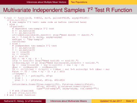
Multivariate Independent Samples T 2 Test R FunctionT.test <- function(X, Y=NULL, mu=0, paired=FALSE, asymp=FALSE){

if(is.null(Y)){# one-sample T^2 test: same code as before (omitted here)

} else {if(paired){

# dependent two-sample T^2 testX <- as.matrix(X)Y <- as.matrix(Y)if(!identical(dim(X),dim(Y))) stop("Need dim(X) == dim(Y).")xx <- T.test(X-Y, mu=mu, asymp=asymp)xx$type <- "dep-sample"return(xx)

} else {# independent two-sample T^2 testX <- as.matrix(X)Y <- as.matrix(Y)nx <- nrow(X)ny <- nrow(Y)p <- ncol(X)df2 <- nx + ny - p - 1if(p != ncol(Y)) stop("Need ncol(X) == ncol(Y).")if(min(nx,ny) <= p) stop("Need min(nrow(X),nrow(Y)) > ncol(X).")Sp <- ((nx-1)*cov(X) + (ny-1)*cov(Y)) / (nx + ny - 2)dbar <- colMeans(X) - colMeans(Y)T2 <- (1/((1/nx) + (1/ny))) * t(dbar - mu) %*% solve(Sp) %*% (dbar - mu)Fstat <- T2 / ((nx + ny - 2) * p / df2)if(asymp){

pval <- 1 - pchisq(T2, df=p)} else {

pval <- 1 - pf(Fstat, df1=p, df2=df2)}return(data.frame(T2=as.numeric(T2), Fstat=as.numeric(Fstat),

df1=p, df2=df2, p.value=as.numeric(pval),type="ind-sample", asymp=asymp, row.names=""))

} # end if(paired)} # end if(is.null(Y))

} # end T.test function



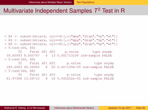
Multivariate Independent Samples T 2 Test in R

> X4 <- subset(mtcars, cyl==4)[,c("mpg","disp","hp","wt")]> X6 <- subset(mtcars, cyl==6)[,c("mpg","disp","hp","wt")]> X8 <- subset(mtcars, cyl==8)[,c("mpg","disp","hp","wt")]> T.test(X4, X6)

T2 Fstat df1 df2 p.value type asymp39.60993 8.045767 4 13 0.001713109 ind-sample FALSE> T.test(X4, X8)

T2 Fstat df1 df2 p.value type asymp185.6083 40.34963 4 20 2.627159e-09 ind-sample FALSE> T.test(X6, X8)

T2 Fstat df1 df2 p.value type asymp61.97388 13.04713 4 16 6.545202e-05 ind-sample FALSE



Comparing Finite Sample and Large Sample p-values

# compare finite sample and large sample p-values (n=10)> set.seed(1)> n <- 10> XX <- matrix(rnorm(n*4), n, 4)> YY <- matrix(rnorm(n*4), n, 4)> T.test(XX,YY)

T2 Fstat df1 df2 p.value type asymp3.582189 0.7462893 4 15 0.5754577 ind-sample FALSE

> T.test(XX,YY,asymp=T)T2 Fstat df1 df2 p.value type asymp

3.582189 0.7462893 4 15 0.4654919 ind-sample TRUE




3.286587 0.7964942 4 95 0.5110603 ind-sample TRUE




3.270955 0.8053489 4 195 0.5135473 ind-sample TRUE



Simultaneous CIs for Independent Samples T 2

A 100(1− α)% confidence interval of the form

a′(x̄1 − x̄2)±

√(1n1

+1n2

)a′Spa

√(n1 + n2 − 2)pn1 + n2 − p − 1

Fp,n1+n2−p−1(α)

covers a′(µ1 − µ2) with probability 1− α simultaneously for all a.

With a = ej (the j-th standard basis vector), we have

(x̄1j − x̄2j)±

√(1n1

+1n2

)sjj(p)

√(n1 + n2 − 2)pn1 + n2 − p − 1

Fp,n1+n2−p−1(α)

where sjj(p) is the j-th diagonal element of Sp.



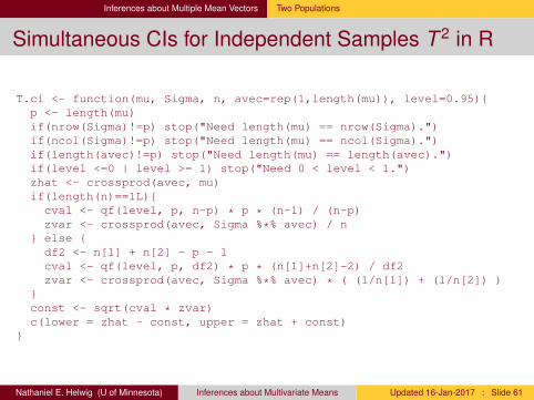
Simultaneous CIs for Independent Samples T 2 in R

T.ci <- function(mu, Sigma, n, avec=rep(1,length(mu)), level=0.95){p <- length(mu)if(nrow(Sigma)!=p) stop("Need length(mu) == nrow(Sigma).")if(ncol(Sigma)!=p) stop("Need length(mu) == ncol(Sigma).")if(length(avec)!=p) stop("Need length(mu) == length(avec).")if(level <=0 | level >= 1) stop("Need 0 < level < 1.")zhat <- crossprod(avec, mu)if(length(n)==1L){cval <- qf(level, p, n-p) * p * (n-1) / (n-p)zvar <- crossprod(avec, Sigma %*% avec) / n

} else {df2 <- n[1] + n[2] - p - 1cval <- qf(level, p, df2) * p * (n[1]+n[2]-2) / df2zvar <- crossprod(avec, Sigma %*% avec) * ( (1/n[1]) + (1/n[2]) )

}const <- sqrt(cval * zvar)c(lower = zhat - const, upper = zhat + const)

}



Example of Simultaneous CIs for Indep. Samples T 2

> X4 <- subset(mtcars, cyl==4)[,c("mpg","disp","hp","wt")]> X6 <- subset(mtcars, cyl==6)[,c("mpg","disp","hp","wt")]> n4 <- nrow(X4)> n6 <- nrow(X6)> dbar <- colMeans(X4) - colMeans(X6)> Sp <- ((n4-1)*cov(X4) + (n6-1)*cov(X6)) / (n4 + n6 - 2)> dbar

mpg disp hp wt6.9207792 -78.1779221 -39.6493506 -0.8314156

> T.ci(dbar, Sp, c(n4,n6), c(1,0,0,0))lower upper

-0.1082001 13.9497585> T.ci(dbar, Sp, c(n4,n6), c(0,1,0,0))

lower upper-141.59106 -14.76478> T.ci(dbar, Sp, c(n4,n6), c(0,0,1,0))

lower upper-82.189575 2.890874> T.ci(dbar, Sp, c(n4,n6), c(0,0,0,1))

lower upper-1.7885075 0.1256764



T 2 Test with Heterogenous Covariances (Σ1 6= Σ2)

Let xkiiid∼ N(µk ,Σk ) for k ∈ {1,2} and assume that the elements of

{x1i}n1i=1 and {x2i}n2


We cannot define a “distance” measure like T 2, whose distributiondoes not depend on the unknown population parameters Σ1 and Σ2.

Use the modified T 2 statistic with non-pooled covariance matrices

T 2 = (x̄1 − x̄2 − [µ1 − µ2])′[n−1

1 S1 + n−12 S2

]−1(x̄1 − x̄2 − [µ1 − µ2])

where x̄k = 1nk

∑nki=1 xki and Sk = 1

nk−1∑nk

i=1(xki − x̄k )(xki − x̄k )′.



Large and Small Sample T 2 Inferences when Σ1 6= Σ2

If min(n1,n2)− p is large, we can use the large sample approximation:

P[T 2 ≤ χ2p(α)] ≈ 1− α

which (asymptotically) works for non-normal multivariate data too!

If min(n1,n2)− p is small and we assume normality, we can use

T 2 ≈ νpν − p + 1

Fp,ν−p+1

where the degrees of freedom parameter ν is estimated as

ν =p + p2∑2

k=11nk

{tr[(

1nk

SkS−10

)2]

+(

tr[

1nk

SkS−10

])2}

with S0 = 1n1

S1 + 1n2

S2. Note that min(n1,n2) ≤ ν ≤ n1 + n2.Nathaniel E. Helwig (U of Minnesota) Inferences about Multivariate Means Updated 16-Jan-2017 : Slide 64


Add var.equal Option to T 2 Test R FunctionT.test <- function(X, Y=NULL, mu=0, paired=FALSE, asymp=FALSE, var.equal=TRUE){if(is.null(Y)){# one-sample T^2 test: same code as before (omitted here)

} else {if(paired){# dependent two-sample T^2 test: same code as before (omitted here)

} else {# independent two-sample T^2 testX <- as.matrix(X)Y <- as.matrix(Y)nx <- nrow(X)ny <- nrow(Y)p <- ncol(X)if(p != ncol(Y)) stop("Need ncol(X) == ncol(Y).")if(min(nx,ny) <= p) stop("Need min(nrow(X),nrow(Y)) > ncol(X).")dbar <- colMeans(X) - colMeans(Y)if(var.equal){

df2 <- nx + ny - p - 1Sp <- ((nx-1)*cov(X) + (ny-1)*cov(Y)) / (nx + ny - 2)T2 <- (1/((1/nx) + (1/ny))) * t(dbar - mu) %*% solve(Sp) %*% (dbar - mu)Fstat <- T2 / ((nx + ny - 2) * p / df2)

} else {Sx <- cov(X)Sy <- cov(Y)Sp <- (Sx/nx) + (Sy/ny)T2 <- t(dbar - mu) %*% solve(Sp) %*% (dbar - mu)SpInv <- solve(Sp)SxSpInv <- (1/nx) * Sx %*% SpInvSySpInv <- (1/ny) * Sy %*% SpInvnudx <- (sum(diag(SxSpInv %*% SxSpInv)) + (sum(diag(SxSpInv)))^2) / nxnudy <- (sum(diag(SySpInv %*% SySpInv)) + (sum(diag(SySpInv)))^2) / nynu <- (p + p^2) / (nudx + nudy)df2 <- nu - p + 1Fstat <- T2 / (nu * p / df2)

}if(asymp){pval <- 1 - pchisq(T2, df=p)

} else {pval <- 1 - pf(Fstat, df1=p, df2=df2)

}return(data.frame(T2=as.numeric(T2), Fstat=as.numeric(Fstat),

df1=p, df2=df2, p.value=as.numeric(pval),type="ind-sample", asymp=asymp, var.equal=var.equal, row.names=""))

} # end if(paired)} # end if(is.null(Y))

} # end T.test function



Example with var.equal Option

> X4 <- subset(mtcars, cyl==4)[,c("mpg","disp","hp","wt")]> X6 <- subset(mtcars, cyl==6)[,c("mpg","disp","hp","wt")]> T.test(X4, X6)

T2 Fstat df1 df2 p.value type asymp var.equal39.60993 8.045767 4 13 0.001713109 ind-sample FALSE TRUE> T.test(X4, X6, var.equal=FALSE)

T2 Fstat df1 df2 p.value type asymp var.equal46.04706 9.266334 4 12.38026 0.001067989 ind-sample FALSE FALSE

> set.seed(1)> n <- 100> XX <- matrix(rnorm(n*4), n, 4)> YY <- matrix(rnorm(n*4), n, 4)> T.test(XX,YY)

T2 Fstat df1 df2 p.value type asymp var.equal3.270955 0.8053489 4 195 0.5230921 ind-sample FALSE TRUE> T.test(XX,YY,var.equal=F)

T2 Fstat df1 df2 p.value type asymp var.equal3.270955 0.8053198 4 194.537 0.5231144 ind-sample FALSE FALSE


Inferences about Multiple Mean Vectors One-Way Multivariate Analysis of Variance (MANOVA)

Univariate Reminder: One-Way ANOVA

Suppose that xkiind∼ N(µk , σ

2) for k ∈ {1, . . . ,g} and i ∈ {1, . . . ,nk}.

The one-way analysis of variance (ANOVA) model has the form

xki = µ+ αk + εki

where µ is the overall mean, αk is the k -th group’s treatment effect withthe constraint that

∑gk=1 nkαk = 0, and εki

iid∼ N(0, σ2) are error terms.

The sample estimates of the model parameters are

µ̂ = x̄ and α̂k = x̄k − x̄ and ε̂ki = xki − x̄k

where x̄ = 1∑gk=1 nk

∑gk=1 nk x̄k and x̄k = 1

nk

∑nki=1 xki .



Univariate Reminder: One-Way ANOVA (continued)

We want to test the hypotheses H0 : αk = 0 for all k ∈ {1, . . . ,g}versus H1 : αk 6= 0 for some k ∈ {1, . . . ,g}.

The decomposition of the sums-of-squares has the formg∑

k=1

nk∑i=1

(xki − x̄)2

︸︷︷︸SS Total

=

g∑k=1

nk (x̄k − x̄)2

︸︷︷︸SS Between

+

g∑k=1

nk∑i=1

(xki − x̄k )2

︸︷︷︸SS Within

The ANOVA F test rejects H0 at level α if

F =SSB/(g − 1)

SSW/(n − g)> Fg−1,n−g(α)

where n =∑g

k=1 nk .Nathaniel E. Helwig (U of Minnesota) Inferences about Multivariate Means Updated 16-Jan-2017 : Slide 68


Multivariate Extension of One-Way ANOVA

Let xkiiid∼ N(µk ,Σ) for k ∈ {1, . . . ,g} and assume that the elements of

{xki}nki=1 and {x`i}n`


The one-way multivariate analysis of variance (MANOVA) has the form

xki = µ + αk + εki

where µk = µ+αk , µ is the overall mean vector, αk is the k -th group’streatment effect vector (with

∑gk=1 nkαk = 0p), and εki

iid∼ N(0p,Σ).


µ̂ = x̄ and α̂k = x̄k − x̄ and ε̂ki = xki − x̄k

where x̄ = 1∑gk=1 nk

∑gk=1 nk x̄k and x̄k = 1

nk

∑nki=1 xki .



Sums-of-Squares and Crossproducts Decomposition

The MANOVA sums-of-squares and crossproducts decomposition is

g∑k=1

nk∑i=1

(xki − x̄)(xki − x̄)′︸︷︷︸SSCP Total

=

g∑k=1

nk (x̄k − x̄)(x̄k − x̄)′︸︷︷︸SSCP Between

+

g∑k=1

nk∑i=1

(xki − x̄k )(xki − x̄k )′︸︷︷︸SSCP Within

and note that the within SSCP matrix has the form

W =

g∑k=1

nk∑i=1

(xki − x̄k )(xki − x̄k )′

=

g∑k=1

(nk − 1)Sk

where Sk = 1nk−1

∑nki=1(xki − x̄k )(xki − x̄k )′ is the k -th group’s sample

covariance matrix.Nathaniel E. Helwig (U of Minnesota) Inferences about Multivariate Means Updated 16-Jan-2017 : Slide 70


One-Way MANOVA SSCP Table

Similar to the one-way ANOVA, we can summarize the SSCPinformation in a table

Source SSCP Matrix D.F.Between B =

∑gk=1 nk (x̄k − x̄)(x̄k − x̄)′ g − 1

Within W =∑g

k=1∑nk

i=1(xki − x̄k )(xki − x̄k )′∑g

k=1 nk − gTotal B + W =

∑gk=1

∑nki=1(xki − x̄)(xki − x̄)′

∑gk=1 nk − 1

Between = treatment sum-of-squares and crossproductsWithin = residual (error) sum-of-squares and crossproducts



MANOVA Extension of ANOVA F Test

We want to test the hypotheses H0 : αk = 0p for all k ∈ {1, . . . ,g}versus H1 : αk 6= 0p for some k ∈ {1, . . . ,g}.

The MANOVA test statistic has the form

Λ∗ =|W||B + W|

which is known as Wilks’ lambda.

Reject H0 if Λ∗ is smaller than expected under H0.



Distribution for Wilks’ Lambda

For certain special cases, the exact distribution of Λ∗ is known

p g Sampling Distribution

p = 1 g ≥ 2(

n−gg−1

) (1−Λ∗

Λ∗

)∼ Fg−1,n−g

p = 2 g ≥ 2(

n−g−1g−1

)(1−√

Λ∗√Λ∗

)∼ F2(g−1),2(n−g−1)

p ≥ 1 g = 2(

n−p−1p

) (1−Λ∗

Λ∗

)∼ Fp,n−p−1

p ≥ 1 g = 3(

n−p−2p

)(1−√

Λ∗√Λ∗

)∼ F2p,2(n−p−2)

where n =∑g

k=1 nk .

If n is large and H0 is true, then

−(

n − 1− p + g2

)log(Λ∗) ≈ χ2

p(g−1)



Other One-Way MANOVA Test Statistics

There are other popular MANOVA test statisticsLawley-Hotelling trace: tr(BW−1)

Pillai trace: tr(B[B + W]−1)

Roy’s largest root: maximum eigenvalue of W(B + W)−1

Each of these test statistics has a corresponding (approximate)distribution, and all should produce similar inference for large n.

Some evidence that Pillai’s trace is more robust to non-normality



One-Way MANOVA Example in R> X <- as.matrix(mtcars[,c("mpg","disp","hp","wt")])> cylinder <- factor(mtcars$cyl)> mod <- lm(X ~ cylinder)> Manova(mod, test.statistic="Pillai")

Type II MANOVA Tests: Pillai test statisticDf test stat approx F num Df den Df Pr(>F)

cylinder 2 1.0838 7.9845 8 54 4.969e-07 ***---Signif. codes: 0 ‘***’ 0.001 ‘**’ 0.01 ‘*’ 0.05 ‘.’ 0.1 ‘ ’ 1> Manova(mod, test.statistic="Wilks")

Type II MANOVA Tests: Wilks test statisticDf test stat approx F num Df den Df Pr(>F)

cylinder 2 0.091316 15.01 8 52 4e-11 ***---Signif. codes: 0 ‘***’ 0.001 ‘**’ 0.01 ‘*’ 0.05 ‘.’ 0.1 ‘ ’ 1> Manova(mod, test.statistic="Roy")

Type II MANOVA Tests: Roy test statisticDf test stat approx F num Df den Df Pr(>F)

cylinder 2 7.7873 52.564 4 27 2.348e-12 ***---Signif. codes: 0 ‘***’ 0.001 ‘**’ 0.01 ‘*’ 0.05 ‘.’ 0.1 ‘ ’ 1> Manova(mod, test.statistic="Hotelling-Lawley")

Type II MANOVA Tests: Hotelling-Lawley test statisticDf test stat approx F num Df den Df Pr(>F)

cylinder 2 8.0335 25.105 8 50 5.341e-15 ***---Signif. codes: 0 ‘***’ 0.001 ‘**’ 0.01 ‘*’ 0.05 ‘.’ 0.1 ‘ ’ 1


Inferences about Multiple Mean Vectors Simultaneous Confidence Intervals for Treatment Effects

Variance of Treatment Effect Difference

Let αkj denote the j-th element of αk and note that

α̂kj = x̄kj − x̄j

where x̄j = 1∑gk=1 nk

∑gk=1 nk x̄kj and x̄kj = 1

nk

∑nki=1 xkij

x̄kj is the k -th group’s mean for the j-th variablex̄j is the overall mean of the j-th variable

The variance for the difference in the estimated treatment effects is

Var(α̂kj − α̂`j) = Var(x̄kj − x̄`j) =

(1nk

+1n`

)σjj

where σjj is the j-th diagonal element of Σ.



Forming Simultaneous CIs via Bonferroni’s Method

To estimate the variance for the treatment effect difference, we use

V̂ar(α̂kj − α̂`j) =

(1nk

+1n`

)wjj

n − g

where wjj denotes the j-th diagonal of W.

We can use Bonferroni’s method to control the familywise error rateHave p variables and g(g − 1)/2 pairwise comparisonsTotal of q = pg(g − 1)/2 tests to control forUse critical values tn−g(α/[2q]) = tn−g(α/[pg(g − 1)])



Get Least-Squares MANOVA Means in R

# get least-squares means for each variable> library(lsmeans)> p <- ncol(X)> lsm <- vector("list", p)> names(lsm) <- colnames(X)> for(j in 1:p){+ wts <- rep(0, p)+ wts[j] <- 1+ lsm[[j]] <- lsmeans(mod, "cylinder", weights=wts)+ }

> lsm[[1]]cylinder lsmean SE df lower.CL upper.CL4 26.66364 0.9718008 29 24.67608 28.651196 19.74286 1.2182168 29 17.25132 22.234398 15.10000 0.8614094 29 13.33822 16.86178

Results are averaged over the levels of: rep.measConfidence level used: 0.95

> lsm[[3]]cylinder lsmean SE df lower.CL upper.CL4 82.63636 11.43283 29 59.25361 106.01916 122.28571 14.33181 29 92.97388 151.59758 209.21429 10.13412 29 188.48769 229.9409




Form Simultaneous Confidence Intervals in R

# get alpha level for Bonferroni correction> q <- p * 3 * (3-1) / 2> alpha <- 0.05 / (2*q)

# Bonferroni pairwise CIs for "mpg"> confint(contrast(lsm[[1]], "pairwise"), level=1-alpha, adj="none")contrast estimate SE df lower.CL upper.CL4 - 6 6.920779 1.558348 29 1.6526941 12.1888644 - 8 11.563636 1.298623 29 7.1735655 15.9537076 - 8 4.642857 1.492005 29 -0.4009503 9.686665


# Bonferroni pairwise CIs for "hp"> confint(contrast(lsm[[3]], "pairwise"), level=1-alpha, adj="none")contrast estimate SE df lower.CL upper.CL4 - 6 -39.64935 18.33331 29 -101.6261 22.327444 - 8 -126.57792 15.27776 29 -178.2252 -74.930606 - 8 -86.92857 17.55281 29 -146.2668 -27.59031



Inferences about Multiple Mean Vectors Testing for Equal Covariance Matrices

Testing the Homogeneity of Covariances Assumption

The one-way MANOVA model assumes that Σ1 = · · · = Σg .

To test H0 : Σ1 = · · · = Σg versus H1 : Σk 6= Σ` for somek , ` ∈ {1, . . . ,g}, we use the likelihood ratio test (LRT) statistic

Λ =

g∏k=1

(|Sk ||SP |

)(nk−1)/2

where SP = 1n−g W is the pooled covariance matrix estimate.

It was shown (by George Box) that −2 log(Λ) ≈ 11−uχ

2ν where

u =

( g∑k=1

1nk− 1

n

)(2p2 + 3p − 1

6(p + 1)(g − 1)

)ν = p(p + 1)(g − 1)/2


Inferences about Multiple Mean Vectors Testing for Equal Covariance Matrices

Testing Homogeneity of Covariances in R

> library(biotools)> boxM(X, cylinder)

Box’s M-test for Homogeneity of Covariance Matrices

data: XChi-Sq (approx.) = 40.851, df = 20, p-value = 0.003892

We reject the null hypothesis that Σ1 = · · · = Σg , so our previousMANOVA results may be invalid.

M-test is sensitive to non-normality, so it may be ok to proceed with theMANOVA in some cases when the M-test rejects the null hypothesis.


Inferences about Multiple Mean Vectors Two-Way Multivariate Analysis of Variance (MANOVA)

Univariate Reminder: Two-Way ANOVA

x`kiind∼ N(µk`, σ

2) for k ∈ {1, . . . ,a}, ` ∈ {1, . . . ,b}, and i ∈ {1, . . . ,n}.

The two-way analysis of variance (ANOVA) model has the form

x`ki = µ+ αk + β` + γk` + ε`ki

whereµ is the overall meanαk is the main effect for factor 1 (

∑ak=1 αk = 0)

β` is the main effect for factor 2 (∑b

`=1 β` = 0)γk` is the interaction effect between factors 1 and 2(∑a

k=1 γk` =∑b

`=1 γk` = 0)

ε`kiiid∼ N(0, σ2) are error terms



Univariate Reminder: Two-Way ANOVA Estimation

The two-way ANOVA model implies the decomposition

x`ki = x̄︸︷︷︸µ̂

+ (x̄k · − x̄)︸︷︷︸α̂k

+ (x̄·` − x̄)︸︷︷︸β̂`

+ (x̄k` − x̄k · − x̄·` + x̄)︸︷︷︸γ̂k`

+ (x`ki − x̄k`)︸︷︷︸ε̂`ki

wherex̄ = 1

abn∑a

k=1∑b

`=1∑n

i=1 x`ki is the overall mean

x̄k · = 1bn∑b

`=1∑n

i=1 x`ki is the mean of k -th level of factor 1

x̄·` = 1an∑a

k=1∑n

i=1 x`ki is the mean of `-th level of factor 2

x̄k` = 1n∑n

i=1 x`ki is the mean of the k -th level of factor 1 and the`-th level of factor 2



Univariate Reminder: Two-Way ANOVA Sum-of-Sq

The two-way ANOVA sum-of-squares decomposition is

a∑k=1

b∑`=1

n∑i=1

(x`ki − x̄)2

︸︷︷︸SSTotal

=a∑

k=1

bn(x̄k · − x̄)2

︸︷︷︸SSA

+b∑`=1

an(x̄·` − x̄)2

︸︷︷︸SSB

+a∑

k=1

b∑`=1

n(x̄k` − x̄k · − x̄·` + x̄)2

︸︷︷︸SSAB

+a∑

k=1

b∑`=1

n∑i=1

(x`ki − x̄k`)2

︸︷︷︸SSError



Univariate Reminder: Two-Way ANOVA Inference

Source Sum-of-Squares D.F.Factor 1

∑ak=1 bn(x̄k · − x̄)2 a− 1

Factor 2∑b

`=1 an(x̄·` − x̄)2 b − 1Interaction

∑ak=1

∑b`=1 n(x̄k` − x̄k · − x̄·` + x̄)2 (a− 1)(b − 1)

Error∑a

k=1∑b

`=1∑n

i=1(x`ki − x̄k`)2 ab(n − 1)

Total∑a

k=1∑b

`=1∑n

i=1(x`ki − x̄)2 abn − 1

Reject H0 : α1 = · · · = αa = 0 if SSAa−1 > Fa−1,ab(n−1)(α)

Reject H0 : β1 = · · · = βb = 0 if SSBb−1 > Fb−1,ab(n−1)(α)

Reject H0 : γ11 = · · · = γk` = 0 if SSAB(a−1)(b−1) > F(a−1)(b−1),ab(n−1)(α)



Multivariate Extension of Two-Way ANOVA

x`kiind∼ N(µk`,Σ) for k ∈ {1, . . . ,a}, ` ∈ {1, . . . ,b}, and i ∈ {1, . . . ,n}.

The two-way multivariate analysis of variance (MANOVA) has the form

x`ki = µ + αk + β` + τ k` + ε`ki

where the terms are analogues of those in the two-way ANOVA model.


x`ki = x̄︸︷︷︸µ̂

+ (x̄k · − x̄)︸︷︷︸α̂k

+ (x̄·` − x̄)︸︷︷︸β̂`

+ (x̄k` − x̄k · − x̄·` + x̄)︸︷︷︸γ̂k`

+ (x`ki − x̄k`)︸︷︷︸ε̂`ki

where the terms are analogues of those in the two-way ANOVA model.



Two-Way MANOVA Table

Source SSCP D.F.Factor 1

∑ak=1 bn(x̄k · − x̄)(x̄k · − x̄)′ a− 1

Factor 2∑b

`=1 an(x̄·` − x̄)(x̄·` − x̄)′ b − 1Interaction

∑ak=1

∑b`=1 nx̃k`x̃′k` (a− 1)(b − 1)

Error∑a

k=1∑b

`=1∑n

i=1(x`ki − x̄k`)(x`ki − x̄k`)′ ab(n − 1)

Total∑a

k=1∑b

`=1∑n

i=1(x`ki − x̄)(x`ki − x̄)′ abn − 1where x̃k` = (x̄k` − x̄k · − x̄·` + x̄).

SSCPT = SSCPA + SSCPB + SSCPAB + SSCPE



Two-Way MANOVA Inference

Reject H0 : α1 = · · · = αa = 0p if νA log(Λ∗A) > χ2(a−1)p(α)

Λ∗A = |SSCPE ||SSCPA + SSCPE | and νA = −

[ab(n − 1)− p+1−(a−1)

2

]

Reject H0 : β1 = · · · = βb = 0p if νB log(Λ∗B) > χ2(b−1)p(α)

Λ∗B = |SSCPE ||SSCPB + SSCPE | and νB = −

[ab(n − 1)− p+1−(b−1)

2

]

Reject H0 : γ11 = · · · = γk` = 0p if νAB log(Λ∗AB) > χ2(a−1)(b−1)p(α)

Λ∗AB = |SSCPE ||SSCPAB + SSCPE | and νAB = −

[ab(n − 1)− p+1−(a−1)(b−1)

2

]

Use tab(n−1) distribution with Bonferroni correction for CIs.Nathaniel E. Helwig (U of Minnesota) Inferences about Multivariate Means Updated 16-Jan-2017 : Slide 88


Two-Way MANOVA Example in R (fit model)

# two-way manova with interaction> data(mtcars)> X <- as.matrix(mtcars[,c("mpg","disp","hp","wt")])> cylinder <- factor(mtcars$cyl)> transmission <- factor(mtcars$am)> mod <- lm(X ~ cylinder * transmission)> Manova(mod, test.statistic="Wilks")


cylinder 2 0.09550 12.8570 8 46 1.689e-09 ***transmission 1 0.43720 7.4019 4 23 0.0005512 ***cylinder:transmission 2 0.58187 1.7880 8 46 0.1040156---Signif. codes: 0 ‘***’ 0.001 ‘**’ 0.01 ‘*’ 0.05 ‘.’ 0.1 ‘ ’ 1

# refit additive model> mod <- lm(X ~ cylinder + transmission)> Manova(mod, test.statistic="Wilks")


cylinder 2 0.11779 11.9610 8 50 2.414e-09 ***transmission 1 0.49878 6.2805 4 25 0.001217 **---Signif. codes: 0 ‘***’ 0.001 ‘**’ 0.01 ‘*’ 0.05 ‘.’ 0.1 ‘ ’ 1



Two-Way MANOVA Example in R (get LS means)> p <- ncol(X)> lsm.cyl <- lsm.trn <- vector("list", p)> names(lsm) <- colnames(X)> for(j in 1:p){+ wts <- rep(0, p*2)+ wts[1:2 + (j-1)*2] <- 1+ lsm.cyl[[j]] <- lsmeans(mod, "cylinder", weights=wts)+ wts <- rep(0, p*3)+ wts[1:3 + (j-1)*3] <- 1+ lsm.trn[[j]] <- lsmeans(mod, "transmission", weights=wts)+ }

# print mpg LS mean for cylinder effect> lsm.cyl[[1]]cylinder lsmean SE df lower.CL upper.CL4 26.08183 0.9724817 28 24.08979 28.073876 19.92571 1.1653575 28 17.53858 22.312848 16.01427 0.9431293 28 14.08236 17.94618

Results are averaged over the levels of: transmission, rep.measConfidence level used: 0.95

# print mpg LS mean for transmission effect> lsm.trn[[1]]transmission lsmean SE df lower.CL upper.CL0 19.39396 0.7974085 28 17.76054 21.027381 21.95391 0.9283388 28 20.05230 23.85553

Results are averaged over the levels of: cylinder, rep.measConfidence level used: 0.95



Two-Way MANOVA Example in R (simultaneous CIs)

# get alpha level for Bonferroni correction> q <- p * (3 * (3-1) / 2 + 2 * (2-1) / 2)> alpha <- 0.05 / (2*q)

# Bonferroni pairwise CIs for "mpg" (cylinder effect)> confint(contrast(lsm.cyl[[1]], "pairwise"), level=1-alpha, adj="none")contrast estimate SE df lower.CL upper.CL4 - 6 6.156118 1.535723 28 0.7758311 11.5364044 - 8 10.067560 1.452082 28 4.9803008 15.1548186 - 8 3.911442 1.470254 28 -1.2394803 9.062364

Results are averaged over the levels of: transmission, rep.measConfidence level used: 0.9984375

# Bonferroni pairwise CIs for "mpg" (tranmission effect)> confint(contrast(lsm.trn[[1]], "pairwise"), level=1-alpha, adj="none")contrast estimate SE df lower.CL upper.CL0 - 1 -2.559954 1.297579 28 -7.105921 1.986014

Results are averaged over the levels of: cylinder, rep.measConfidence level used: 0.9984375


nathaniel e. helwig - school of statisticsusers.stat.umn.edu/~helwig/notes/mvmean-notes.pdf · t2...

Documents