national grid emr national grid electricity capacity … news...page 6 of 117 national grid emr...
TRANSCRIPT
Page 1 of 117 National Grid EMR Electricity Capacity Report 2016
National Grid
1.
National Grid EMRElectricity Capacity Report
31st May 2016 (submitted to DECC)
Report with results from work undertaken by National Grid for DECC in order to support thedevelopment of Capacity Market volume to secure.

Page 2 of 117 National Grid EMR Electricity Capacity Report 2016
Disclaimer
This Electricity Capacity Report (ECR) has been prepared solely for the purpose ofthe Electricity Market Reform (EMR) Capacity Market and is not designed or intendedto be used for any other purpose. Whilst National Grid Electricity Transmission(NGET), in its role as EMR Delivery Body and is thereafter referred to as NationalGrid in this report, has taken all reasonable care in its preparation, no representationor warranty either express or implied is made as to the accuracy or completeness ofthe information that it contains and parties using that information should make theirown enquiries as to its accuracy and suitability for the purpose for which they use it.Save in respect of liability for death or personal injury caused by its negligence orfraud or for any other liability which cannot be excluded or limited under applicablelaw, neither National Grid nor any other companies in the National Grid plc group, norany Directors or employees of any such company shall be liable for any losses,liabilities, costs, damages or claims arising (whether directly or indirectly) as a resultof the content of, use of or reliance on any of the information contained in the report.
Confidentiality
National Grid Electricity Transmission plc (“NGET”) has conducted this work inaccordance with the requirements of Special Condition 2N (Electricity MarketReform) of the NGET transmission licence and the Compliance Statementestablished under that condition that has been approved by the Gas and ElectricityMarkets Authority. This condition imposes on NGET obligations of confidentiality andnon-disclosure in respect of confidential EMR information. Non-compliance withSpecial Condition 2N or the Compliance Statement will constitute a breach of theNGET transmission licence.
Contact
Any enquiries regarding this publication should be sent to National Grid [email protected]
Page 3 of 117 National Grid EMR Electricity Capacity Report 2016
National Grid EMR Electricity CapacityReport
1. Executive Summary..............................................................61.1 Modelling Process .......................................................................61.2 National Grid Analysis Delivery Timeline 2016 ...................71.3 Results and Recommendations...............................................7
1.3.1 2020/21 T-4 Auction Recommendation........................................................81.3.2 2017/18 Early Auction Recommendation...................................................111.3.3 2018/19 Indicative Requirement for T-1 Auction ......................................13
1.4 Interconnected Countries De-rating factor Ranges .........152. The Modelling Approach .....................................................16
2.1 High Level Approach ................................................................162.2 Stakeholder Engagement ........................................................172.3 High Level Assumptions..........................................................18
2.3.1 Interconnector Assumptions .......................................................................182.3.2 Station Availabilities...................................................................................18
2.4 DDM Outputs Used in the ECR ..............................................222.5 PTE Recommendations............................................................222.6 Modelling Enhancements since Last Report .....................27
2.6.1 Data Input Assumptions..............................................................................272.6.2 Modelling Changes .....................................................................................292.6.3 Interpretation of Results..............................................................................31
2.7 Quality Assurance .....................................................................323. Scenarios & Sensitivities ....................................................33
3.1 Overview.......................................................................................333.2 Scenario Descriptions ..............................................................34
3.2.1 Gone Green .................................................................................................343.2.2 Slow Progression ........................................................................................353.2.3 No Progression............................................................................................353.2.4 Consumer Power.........................................................................................36
3.3 Demand Forecast until 2020/21..............................................363.4 Demand Forecast 2021/22 onwards .....................................373.5 Demand Methodology ..............................................................38
3.5.1 Domestic .....................................................................................................393.5.2 Industrial .....................................................................................................393.5.3 Commercial.................................................................................................393.5.4 Other/Sundry...............................................................................................403.5.5 Peak Demands.............................................................................................403.5.6 Calibration...................................................................................................403.5.7 Results.........................................................................................................403.5.8 Demand Side Response...............................................................................413.5.9 Power Responsive.......................................................................................43
3.6 Generation Capacity until 2020/21 ........................................44
Page 4 of 117 National Grid EMR Electricity Capacity Report 2016
3.7 Generation Capacity 2021/22 onwards ................................453.8 Distributed Generation .............................................................463.9 Generation Methodology .........................................................48
3.9.1 Contracted Background ..............................................................................483.9.2 Market Intelligence .....................................................................................483.9.3 FES Plant Economics..................................................................................493.9.4 Project Status ..............................................................................................503.9.5 Government Policy and Legislation............................................................503.9.6 Reliability Standard ....................................................................................51
3.10 Interconnector Capacity Assumptions..............................513.11 Sensitivity Descriptions and Justifications .....................54
3.11.1 Low Wind (at times of cold weather) .......................................................543.11.2 High Wind (at times of cold weather).......................................................553.11.3 High Plant Availabilities...........................................................................553.11.4 Low Plant Availabilities ...........................................................................553.11.5 Interconnector Assumptions & Sensitivities (2018/19 only)....................563.11.6 Weather – Cold Winter .............................................................................563.11.7 Weather – Warm Winter...........................................................................573.11.8 High Demand ............................................................................................573.11.9 Low Demand.............................................................................................583.11.10 Non-delivery of Contracted Coal Capacity.............................................583.11.11 Sensitivities Considered but Rejected.....................................................58
3.12 15 years horizon.......................................................................594. De-rating Factors for CM Auctions ......................................61
4.1 Conventional Plants ..................................................................614.2 DSR De-rating Factor ................................................................624.3 Interconnectors ..........................................................................63
4.3.1 Methodology...............................................................................................634.3.2 Baringa Pan-European Model Results ........................................................644.3.3 Validation/ Comparison/Other Analysis.....................................................664.3.4 Pöyry historical analysis .............................................................................674.3.5 Country de-ratings ......................................................................................68
5. Results and Recommendation for 2020/21 T-4 Auction .......765.1 Sensitivities to model ...............................................................765.2 Results ..........................................................................................765.3 Recommended Capacity to Secure ......................................77
5.3.1 Covered range .............................................................................................795.3.2 Adjustments to Recommended Capacity ....................................................79
6. Results and Recommendation for 2017/18 Early Auction ....816.1 Sensitivities to model ...............................................................816.2 Results ..........................................................................................816.3 Recommended Capacity to Secure ......................................82
6.3.1 Covered range .............................................................................................836.3.2 Adjustments to Recommended Capacity ....................................................84
7. Results and Indicative T-1 Requirement for 2018/19 Auction..............................................................................................85
Page 5 of 117 National Grid EMR Electricity Capacity Report 2016
7.1 Sensitivities to model ...............................................................857.2 Results ..........................................................................................857.3 Indicative Capacity to Secure.................................................86
7.3.1 Covered range .............................................................................................877.3.2 Adjustments to Indicative Capacity ............................................................887.3.3 Comparison with 2018/19 recommendation...............................................88
A. Annex ................................................................................91A.1 Future Energy Scenario Method ...........................................91A.2 Detailed Modelling Assumptions..........................................92
A.2.1 Demand (annual and peak) ........................................................................92A.2.2 Generation Mix ..........................................................................................93A.2.3 CM-ineligible Capacity..............................................................................95A.2.4 Station Availabilities..................................................................................96A.2.5 Reserve to cover largest infeed loss ...........................................................98
A.3 Detailed Modelling Approach ................................................98A.3.1 Using DDM to model capacity to secure ...................................................98A.3.2 Treatment of Generation Technologies....................................................102
A.4 Least Worst Regret .................................................................104A.4.1 Approach..................................................................................................104A.4.2 Worked Example......................................................................................105A.4.3 Capacity to Secure Charts ........................................................................107
A.5 Quality Assurance...................................................................110

Page 6 of 117 National Grid EMR Electricity Capacity Report 2016
1. Executive Summary
This Electricity Capacity Report (ECR) summarises the modelling analysisundertaken by National Grid in its role as the Electricity Market Reform (EMR)Delivery Body to support the decision by the Government on the amount of capacityto secure through the Capacity Market auctions for delivery in 2017/18 and 2020/21.
In addition we have been asked by Department of Energy and Climate Change(DECC) to provide, for information only, an early snapshot of an indicativerequirement for the 2018/19 T-1 auction that will improve transparency and helpmarket participants understand their options more clearly.
The Government requires National Grid to provide it with a recommendation for eachyear studied based on the analysis of a number of scenarios and sensitivities that willensure its policy objectives are achieved in a cost effective manner.
Chapter 2 of this report aims to describe the modelling approach and the toolsutilised. Chapter 3 of the report describes the individual scenarios and sensitivitiesmodelled. Chapter 4 covers the modelling and recommendation for the de-ratingfactors to apply to interconnectors and conventional plants. Chapter 5 containsresults from the scenarios modelled, along with a recommended capacity to securefor the 2020/21 T-4 auction. Chapter 6 provides recommended capacity to secure forthe 2017/18 early auction. Chapter 7 provides an indicative capacity requirement forthe 2018/19 T-1 auction. Finally the Annex contains the details behind theassumptions, the modelling approach, a least worst regret example and the qualityassurance process.
1.1 Modelling Process
A key aim of this analysis is to provide advice to the Government on how differentscenarios would impact on its objectives, so that it can take informed decisions. Themodelling approach adopted for the EMR Capacity Market analysis is described indetail in the Annex, including the data, assumptions and models utilised. Thescenarios and sensitivities run through the model are detailed in Chapter 3. Thescenarios and sensitivities investigated offer a range of likely demand and generationoutcomes which are intended to meet the required security of supply as set out byGovernment’s Reliability Standard.
The principal modelling tool National Grid has used is a fully integrated power marketmodel, the Dynamic Dispatch Model (DDM). The model enables analysis of electricitydispatch from power generators and investment decisions in generating capacity toat least 2035. The model performs runs based on sample days, including demandload curves for both business and non-business days. Investment decisions arebased on projected revenue and cash flows allowing for policy impacts and changesin the generation mix and interconnection capacity. The full lifecycle of powergeneration plant is modelled through to decommissioning endeavouring to replicatethe real world investment decisions without perfect foresight as the model isn’toptimised.
In order to provide the most complete view of the implications of the alternativescenarios and sensitivities (see the results in Chapter 5, 6 & 7), National Grid hasalso built a “Least Worst Regret (LWR)” tool to calculate the appropriate level of

Page 7 of 117 National Grid EMR Electricity Capacity Report 2016
capacity to secure to meet the Reliability Standard that minimises the regret costimplications of that decision.
National Grid has also considered the recommendations included in the Panel ofTechnical Experts (PTE) report on the 2015 process and adjusted and improved thisyear’s analysis appropriately to try to address their feedback. In addition there hasbeen a series of workshops with DECC, PTE and Office of Gas and ElectricityMarkets (Ofgem) to enable them to scrutinise the modelling approach andassumptions utilised.
1.2 National Grid Analysis Delivery Timeline 2016
The process and modelling analysis has been undertaken by National Grid withongoing discussions with DECC, Ofgem and DECC’s PTE during the development,modelling and result phases.
The work was carried out between September 2015 and May 2016 and builds on theanalysis that was undertaken for the previous ECRs. In addition to the analysisaround the recommended capacity to secure, the report also presents analysis onthe de-rating factors for interconnectors and conventional plants to use in theauctions.
The following timeline illustrates the key milestones over the different modellingphases of the work to the publication of the ECR:
Development plan produced in September 2015 Development projects completed by March 2016 Production plan developed in February 2016 Modelling analysis February to May 2016 National Grid’s ECR is sent to DECC before 1st June 2016 Publication of ECR in line with DECC publishing auction parameters planned by
1st July 2016
1.3 Results and Recommendations
National Grid has modelled a range of capacity options based around meeting theReliability Standard in different combinations of credible scenarios and sensitivities.The assumption is that the Future Energy Scenarios (FES) and the Base Case willcover uncertainty by incorporating ranges for annual and peak demand, DemandSide Response (DSR), interconnection capacity and generation with the sensitivitiescovering uncertainty in non-delivery of coal plant, station peak availabilities, weather,wind levels and peak demand forecast range (based on the Peak National DemandForecasting Accuracy (DFA) Incentive1) plus interconnector flow sensitivities (for2018/19 only). In addition to the four FES scenarios and National Grid’s Base Case(see Chapter 3), a DECC Scenario has been included for information but wasexcluded from the LWR calculation to ensure the recommendation is fullyindependent.
1 See Special Condition 4L athttps://epr.ofgem.gov.uk/Content/Documents/National%20Grid%20Electricity%20Transmission%20Plc%20-%20Special%20Conditions%20-%20Current%20Version.pdf
Page 8 of 117 National Grid EMR Electricity Capacity Report 2016
Scenarios & Base Case
Base Case (5 year forecast to 2020/21 then Slow Progression from 2021/22onwards
FES Gone Green (GG) FES Slow Progression (SP) FES No Progression (NP) FES Consumer Power (CP)
To provide the reference case which is being used to apply sensitivities, a Base Casehas been introduced. For the DFA incentive years up to 2020/21, this consists of aforecast of demand and a generation background which aligns with our DFAIncentive and aims to reduce the likelihood of over or under securing of the capacitythereby minimising the associated costs to consumers.
The Base Case also assumes that some capacity contracted in previous T-4 auctionsis not able to honour its awarded contracts. For example, the Base Case assumesearly closures of some contracted coal plants (due to the challenging economicclimate for coal station operators) and the slippage of some new build capacity. Thevolume of such capacity totals 4.3 GW in 2018/19 and 2.9 GW in 2020/21.
While the FES scenarios vary many variables (see list of primary assumptions inAnnex), the sensitivities vary only one variable at a time. Each of the sensitivities isconsidered credible and is evidence based i.e. it has occurred in recent history or isto address statistical uncertainty caused by the small sample sizes used for some ofthe input variables. Section 3.11 describes each sensitivity and how it has beenimplemented.
The LWR methodology is explained in the Annex. As per previous ECR analysis, ituses a cost of capacity of £49/kW/yr and an energy unserved cost of £17,000/MWhto select a scenario/sensitivity combination from which the recommended capacity tosecure is derived. Note that the Government’s Reliability Standard2 was derivedusing a slightly different capacity cost of £47/kW/yr based on the gross Cost of NewEntry (CONE) of an Open Cycle Gas Turbine (OCGT).
1.3.1 2020/21 T-4 Auction Recommendation
Sensitivities
The agreed sensitivities to model (see 3.11 for more details) for 2020/21 cover non-delivery of coal plant, weather, plant availability and demand:
Low Wind Output at times of cold weather (LOW WIND) High Wind Output at times of cold weather (HIGH WIND) Weather Cold Winter (COLD) Weather Warm Winter (WARM) High Plant Availabilities (HIGH AVAIL) Low Plant Availabilities (LOW AVAIL) High Demand (HIGH DEMAND) Low Demand (LOW DEMAND)
2See https://www.gov.uk/government/uploads/system/uploads/attachment_data/file/267613/Annex_C_-
_reliability_standard_methodology.pdf
Page 9 of 117 National Grid EMR Electricity Capacity Report 2016
Non Delivery (NON DEL): 9 sensitivities in 400 MW increments (forgranularity) up to 3600 MW.
Results
The outcome of the Least Worst Regret calculation applied to all of National Grid’sscenarios and sensitivities is an initial capacity to secure for 2020/21 of 49.5 GW(49.48 GW before rounding) based on the Consumer Power scenario. As this is aFES scenario, a small adjustment is required to bring it into line with the DFAIncentive by selecting the nearest Base Case sensitivity based on the DFA Incentivedemand level (See Section 2.6.3 for more details). In this case the nearest sensitivityis the 2000 MW non-delivery sensitivity (49.65 GW before rounding) that ismarginally closer than the 1600 MW non-delivery sensitivity (49.25 GW beforerounding)
This leads to a recommended capacity to secure for 2020/21 of 49.7 GW set by therequirement of the Base Case 2000MW non-delivery sensitivity. This does not takeaccount of a different clearing price to net CONE resulting from the auction as ourrecommended target capacity to secure corresponds to the value on the CM demandcurve for the net CONE capacity cost and also excludes any capacity secured inearlier auctions for 2020/21 that is assumed in the Base Case.
In general, when compared to the analysis for 2019/20 in the 2015 ECR, the 2016scenarios and sensitivities for 2020/21 contain higher levels of CM-ineligible de-ratedcapacity at peak due to higher contribution from renewables (see Annex forbreakdown), in part due to the new offshore power curve (see 2.6.1), as well ashigher levels of assumed ineligible autogeneration below 2 MW3. However thereduction in total CM-eligible capacity requirement due to higher levels of ineligiblecapacity is offset by using a wider range of non-delivery sensitivities that increasesthe requirement in the LWR analysis. The warm winter sensitivity is key to the LWRresult, as it is the sensitivity that sets the highest regret cost for the recommendedcapacity level (see Annex for more details on how regret costs are determined in theLWR calculation).
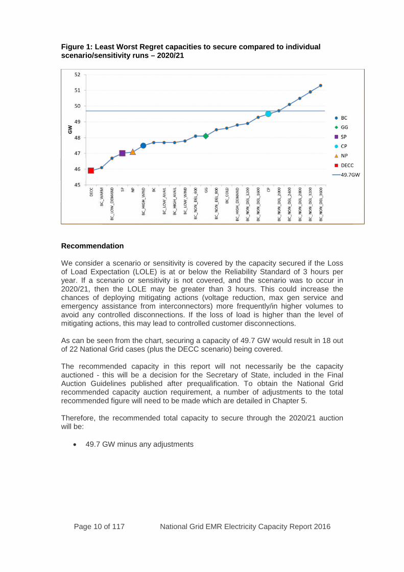
The following chart illustrates the full range of potential capacity levels (from NationalGrid scenarios, Base Case and sensitivities) plus the DECC scenario and identifiesthe Least Worst Regret recommended capacity. Note that National Grid’srecommendation concentrates on the target capacity alone. The values for all of theauction parameters will be determined by the Secretary of State.
3Note that unsupported capacity under 2 MW can enter the auction if it is combined with other capacity by an aggregator to give a
total above 2 MW.
Page 10 of 117 National Grid EMR Electricity Capacity Report 2016
Figure 1: Least Worst Regret capacities to secure compared to individualscenario/sensitivity runs – 2020/21
Recommendation
We consider a scenario or sensitivity is covered by the capacity secured if the Lossof Load Expectation (LOLE) is at or below the Reliability Standard of 3 hours peryear. If a scenario or sensitivity is not covered, and the scenario was to occur in2020/21, then the LOLE may be greater than 3 hours. This could increase thechances of deploying mitigating actions (voltage reduction, max gen service andemergency assistance from interconnectors) more frequently/in higher volumes toavoid any controlled disconnections. If the loss of load is higher than the level ofmitigating actions, this may lead to controlled customer disconnections.
As can be seen from the chart, securing a capacity of 49.7 GW would result in 18 outof 22 National Grid cases (plus the DECC scenario) being covered.
The recommended capacity in this report will not necessarily be the capacityauctioned - this will be a decision for the Secretary of State, included in the FinalAuction Guidelines published after prequalification. To obtain the National Gridrecommended capacity auction requirement, a number of adjustments to the totalrecommended figure will need to be made which are detailed in Chapter 5.
Therefore, the recommended total capacity to secure through the 2020/21 auctionwill be:
49.7 GW minus any adjustments
Page 11 of 117 National Grid EMR Electricity Capacity Report 2016
1.3.2 2017/18 Early Auction Recommendation
Sensitivities
The agreed sensitivities to model (see 3.11) for 2017/18 cover non-delivery, weather,plant availability and demand:
Low Wind Output at times of cold weather (LOW WIND) High Wind Output at times of cold weather (HIGH WIND) Weather Cold Winter (COLD) Weather Warm Winter (WARM) High Plant Availabilities (HIGH AVAIL) Low Plant Availabilities (LOW AVAIL) High Demand (HIGH DEMAND) Low Demand (LOW DEMAND) Non Delivery (NON DEL): 7 sensitivities in 400 MW increments up to 2800
MW.
Results
The outcome of the Least Worst Regret calculation applied to all of National Grid’sscenarios and sensitivities is a recommended capacity to secure for 2017/18 of 53.8GW set by the requirement of the Base Case Cold Winter sensitivity. This does nottake account of a different clearing price resulting from the auction.
In general, when compared to the analysis for 2018/19 in the 2014 ECR, the 2016scenarios and sensitivities for 2017/18 contain higher levels of CM-ineligible de-ratedcapacity at peak due to higher contribution from renewables (See Annex forbreakdown), in part due to the new offshore power curve, as well as higher levels ofassumed ineligible autogeneration below 2 MW. However the reduction in total CM-eligible capacity requirement due to higher levels of ineligible capacity is offset byhigher peak demands and by using a wider range of non-delivery sensitivities thatincreases the requirement in the LWR analysis. The 2800 MW non-deliverysensitivity is the key to the LWR result as it is the sensitivity that sets the highestregret cost for the recommended capacity level (see Annex for more details on howregret costs are determined in the LWR calculation).
The following chart illustrates the full range of potential capacity levels (from NationalGrid scenarios and sensitivities) plus the DECC scenario and identifies the LeastWorst Regret recommended capacity. Note that National Grid’s recommendationconcentrates on the target capacity alone.
Page 12 of 117 National Grid EMR Electricity Capacity Report 2016
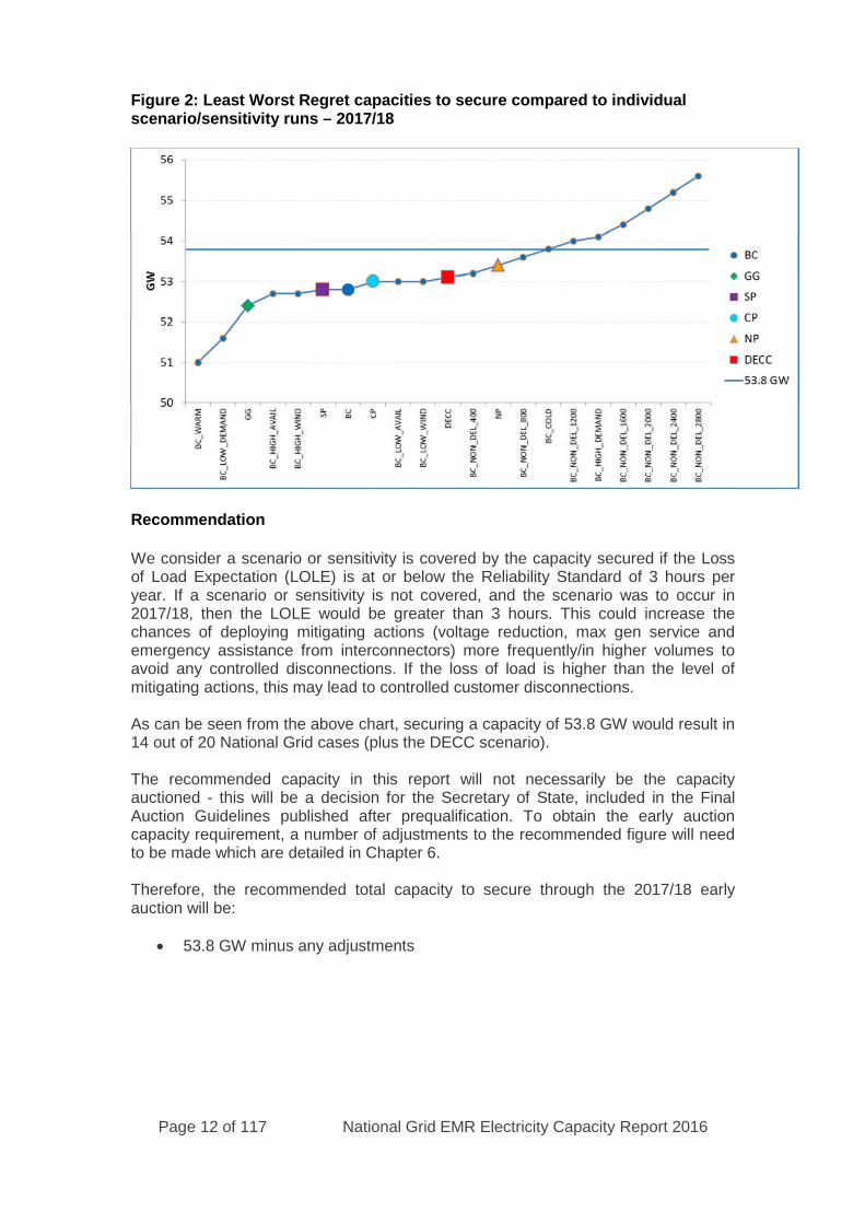
Figure 2: Least Worst Regret capacities to secure compared to individualscenario/sensitivity runs – 2017/18
Recommendation
We consider a scenario or sensitivity is covered by the capacity secured if the Lossof Load Expectation (LOLE) is at or below the Reliability Standard of 3 hours peryear. If a scenario or sensitivity is not covered, and the scenario was to occur in2017/18, then the LOLE would be greater than 3 hours. This could increase thechances of deploying mitigating actions (voltage reduction, max gen service andemergency assistance from interconnectors) more frequently/in higher volumes toavoid any controlled disconnections. If the loss of load is higher than the level ofmitigating actions, this may lead to controlled customer disconnections.
As can be seen from the above chart, securing a capacity of 53.8 GW would result in14 out of 20 National Grid cases (plus the DECC scenario).
The recommended capacity in this report will not necessarily be the capacityauctioned - this will be a decision for the Secretary of State, included in the FinalAuction Guidelines published after prequalification. To obtain the early auctioncapacity requirement, a number of adjustments to the recommended figure will needto be made which are detailed in Chapter 6.
Therefore, the recommended total capacity to secure through the 2017/18 earlyauction will be:
53.8 GW minus any adjustments
Page 13 of 117 National Grid EMR Electricity Capacity Report 2016
1.3.3 2018/19 Indicative Requirement for T-1 Auction
Sensitivities
The agreed sensitivities to model (see 3.11) for 2018/19 cover non-delivery, weather,plant availability, demand and peak interconnector flows:
Low Wind Output at times of cold weather (LOW WIND) High Wind Output at times of cold weather (HIGH WIND) Weather Cold Winter (COLD) Weather Warm Winter (WARM) High Plant Availabilities (HIGH AVAIL) Low Plant Availabilities (LOW AVAIL) High Demand (HIGH DEMAND) Low Demand (LOW DEMAND) Non Delivery (NON DEL): 9 sensitivities in 400 MW increments up to 3600
MW. 750 MW Continental interconnector imports (IC 750IMPORTS): 300 MW net
GB flow (including 450 MW exports to Ireland) 1500 MW Continental interconnector imports (IC 1500IMPORTS): 1300 MW
net GB flow (including 200 MW exports to Ireland) 2250 MW Continental interconnector imports (IC 2250IMPORTS): 2500 MW
net GB flow (including 250 MW imports from Ireland) 3000 MW Continental interconnector imports (IC 3000IMPORTS): 3500 MW
net GB flow (including 500 MW imports from Ireland)
Results
The outcome of the Least Worst Regret calculation applied to all of National Grid’sscenarios and sensitivities is an indicative capacity to secure for 2018/19 of 7.3 GWset by the requirement of the Base Case 1600MW sensitivity (and also the 750 MWContinental Imports sensitivity). This does not take account of a different clearingprice to net CONE resulting from the auction as our indicative target capacity tosecure corresponds to the value on the CM demand curve for the net CONE capacitycost.
In general, when compared to the analysis for 2018/19 in the 2014 ECR, the 2016scenarios and sensitivities for 2018/19 contain higher levels of CM-ineligible de-ratedcapacity at peak due to higher renewables contribution (see Annex for breakdown),higher levels of assumed opted-out or ineligible (below 2 MW) autogeneration, higherimports and over-securing in the 2018/19 T-4 auction. However the reduction in theT-1 CM-eligible capacity requirement due to higher levels of ineligible capacity ismore than offset by assumed non-delivery in the Base Case, the contracted capacityin the T-4 auction being greater than de-rated TEC, “opted out but operational” plantclosing and higher peak demands (See Chapter 7 for more details).
The following chart illustrates the full range of potential capacity levels (from NationalGrid scenarios and sensitivities) plus the DECC scenario and identifies the LeastWorst Regret indicative capacity. Note that this concentrates on the indicative targetcapacity alone.
Page 14 of 117 National Grid EMR Electricity Capacity Report 2016
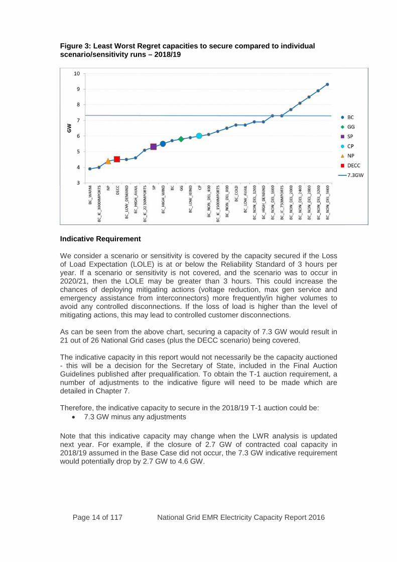
Figure 3: Least Worst Regret capacities to secure compared to individualscenario/sensitivity runs – 2018/19
Indicative Requirement
We consider a scenario or sensitivity is covered by the capacity secured if the Lossof Load Expectation (LOLE) is at or below the Reliability Standard of 3 hours peryear. If a scenario or sensitivity is not covered, and the scenario was to occur in2020/21, then the LOLE may be greater than 3 hours. This could increase thechances of deploying mitigating actions (voltage reduction, max gen service andemergency assistance from interconnectors) more frequently/in higher volumes toavoid any controlled disconnections. If the loss of load is higher than the level ofmitigating actions, this may lead to controlled customer disconnections.
As can be seen from the above chart, securing a capacity of 7.3 GW would result in21 out of 26 National Grid cases (plus the DECC scenario) being covered.
The indicative capacity in this report would not necessarily be the capacity auctioned- this will be a decision for the Secretary of State, included in the Final AuctionGuidelines published after prequalification. To obtain the T-1 auction requirement, anumber of adjustments to the indicative figure will need to be made which aredetailed in Chapter 7.
Therefore, the indicative capacity to secure in the 2018/19 T-1 auction could be: 7.3 GW minus any adjustments
Note that this indicative capacity may change when the LWR analysis is updatednext year. For example, if the closure of 2.7 GW of contracted coal capacity in2018/19 assumed in the Base Case did not occur, the 7.3 GW indicative requirementwould potentially drop by 2.7 GW to 4.6 GW.
Page 15 of 117 National Grid EMR Electricity Capacity Report 2016
1.4 Interconnected Countries De-rating factor Ranges
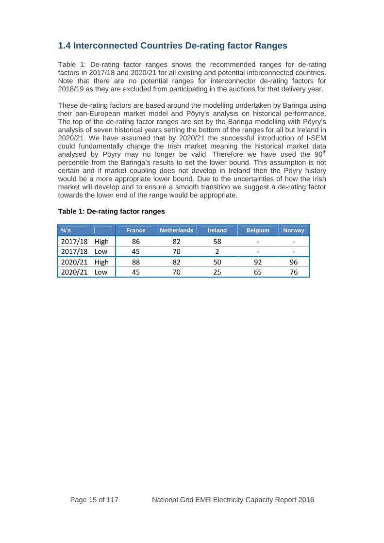
Table 1: De-rating factor ranges shows the recommended ranges for de-ratingfactors in 2017/18 and 2020/21 for all existing and potential interconnected countries.Note that there are no potential ranges for interconnector de-rating factors for2018/19 as they are excluded from participating in the auctions for that delivery year.
These de-rating factors are based around the modelling undertaken by Baringa usingtheir pan-European market model and Pöyry’s analysis on historical performance.The top of the de-rating factor ranges are set by the Baringa modelling with Pöyry’sanalysis of seven historical years setting the bottom of the ranges for all but Ireland in2020/21. We have assumed that by 2020/21 the successful introduction of I-SEMcould fundamentally change the Irish market meaning the historical market dataanalysed by Pöyry may no longer be valid. Therefore we have used the 90th
percentile from the Baringa’s results to set the lower bound. This assumption is notcertain and if market coupling does not develop in Ireland then the Pöyry historywould be a more appropriate lower bound. Due to the uncertainties of how the Irishmarket will develop and to ensure a smooth transition we suggest a de-rating factortowards the lower end of the range would be appropriate.
Table 1: De-rating factor ranges
%’s France Netherlands Ireland Belgium Norway
2017/18 High 86 82 58 - -
2017/18 Low 45 70 2 - -
2020/21 High 88 82 50 92 96
2020/21 Low 45 70 25 65 76

Page 16 of 117 National Grid EMR Electricity Capacity Report 2016
2. The Modelling Approach
The modelling analysis has been undertaken by National Grid with ongoingdiscussions with DECC, Ofgem and DECC’s EMR Panel of Technical Experts (PTE)throughout the whole process.
2.1 High Level Approach
The modelling approach is guided by the policy backdrop, in particular the objectivesset by Government regarding security of supply. The modelling looks to address thefollowing specific question:
What is the volume of capacity to secure that will be required to meet the security ofsupply reliability standard of 3 hours Loss of Load Expectation (LOLE)
4?
In order to answer this question it was agreed, following consultation with DECC andtheir PTE, that the Dynamic Dispatch Model (DDM)5 was an appropriate modellingtool. This maintains consistency with the modelling work undertaken by DECC. TheDDM has the functionality to model the Capacity Market with the following sectionsdescribing this modelling in more detail. It should also be noted that when comparedto National Grid’s capacity assessment model, developed to support Ofgem’sElectricity security of supply report6, the DDM has been shown to produce the sameresults, given the same inputs.
The inputs to the model are in the form of scenarios based on the Future EnergyScenarios (FES)7, and sensitivities around a Base Case which cover a credible andbroad range of possible futures. See Chapter 3 for details of the scenarios andsensitivities used in the modelling. A DECC Scenario has also been included in theanalysis, which provides a point of comparison between DECC’s own analysis andthat contained in this report. The DECC Scenario is based on the reference scenariofrom the 2015 Energy and Emissions Projections8 (EEP). Annual demand projectionsare still consistent with 2015 EEP, but for the purpose of the ECR there have beensome amendments to include the results of the December 2015 Capacity Auctionand to align with National Grid’s 2015 ACS peak.
The scenarios are comprised of assumptions around: Peak demand – Prior to any demand side response Generation capacity – Both transmission connected and distributed (within
the distribution networks) Interconnector assumptions – Capacity assumptions (note that flows at peak
are modelled directly within DDM)
Sensitivities are then created around the Base Case to ensure consistency withNational Grid’s Peak National Demand Forecasting Accuracy (DFA) Incentive9.
4 LOLE is the expected number of hours when demand is higher than available generation during the year but before anymitigating/emergency actions are taken but after all system warnings and SO balancing contracts have been exhausted.5
DDM Release 5.0.0.0 was used for this analysis6 https://www.ofgem.gov.uk/sites/default/files/docs/2015/07/electricitysecurityofsupplyreport_final_0.pdf7
http://fes.nationalgrid.com/8
https://www.gov.uk/government/publications/updated-energy-and-emissions-projections-20159 See Special Condition 4L athttps://epr.ofgem.gov.uk/Content/Documents/National%20Grid%20Electricity%20Transmission%20Plc%20-%20Special%20Conditions%20-%20Current%20Version.pdf
Page 17 of 117 National Grid EMR Electricity Capacity Report 2016
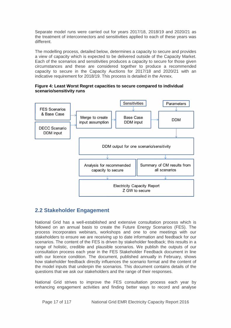
Separate model runs were carried out for years 2017/18, 2018/19 and 2020/21 asthe treatment of interconnectors and sensitivities applied to each of these years wasdifferent.
The modelling process, detailed below, determines a capacity to secure and providesa view of capacity which is expected to be delivered outside of the Capacity Market.Each of the scenarios and sensitivities produces a capacity to secure for those givencircumstances and these are considered together to produce a recommendedcapacity to secure in the Capacity Auctions for 2017/18 and 2020/21 with anindicative requirement for 2018/19. This process is detailed in the Annex.
Figure 4: Least Worst Regret capacities to secure compared to individualscenario/sensitivity runs
2.2 Stakeholder Engagement
National Grid has a well-established and extensive consultation process which isfollowed on an annual basis to create the Future Energy Scenarios (FES). Theprocess incorporates webinars, workshops and one to one meetings with ourstakeholders to ensure we are receiving up to date information and feedback for ourscenarios. The content of the FES is driven by stakeholder feedback; this results in arange of holistic, credible and plausible scenarios. We publish the outputs of ourconsultation process each year in the FES Stakeholder Feedback document in linewith our licence condition. The document, published annually in February, showshow stakeholder feedback directly influences the scenario format and the content ofthe model inputs that underpin the scenarios. This document contains details of thequestions that we ask our stakeholders and the range of their responses.
National Grid strives to improve the FES consultation process each year byenhancing engagement activities and finding better ways to record and analyse

Page 18 of 117 National Grid EMR Electricity Capacity Report 2016
stakeholder feedback. National Grid engages with stakeholders to explain its role inrelation to EMR through the CM Implementation workshops throughout the year.
2.3 High Level Assumptions
There are numerous assumptions which are required for the modelling process.
The starting point for the DDM input modelling assumptions was the set ofassumptions used in the latest DECC modelling e.g. generation levelised costs.However, the key inputs/assumptions are taken by aligning the modelling to the new2016 FES scenarios and agreed sensitivities. The key assumptions are those thatmaterially affect the capacity to secure, these are:
Demand Forecastso Peak demando Annual demand forecasts
Generation Capacityo Capacity eligible for the Capacity Marketo Capacity outside the Capacity Market (including capacity secured
via previous auctions)
For a detailed breakdown of these key input assumptions see the Annex.
2.3.1 Interconnector Assumptions
As part of the UK’s State aid approval for the Capacity Market, interconnectors areeligible to participate in the CM since the 2015 auction. As such, the UK hascommitted to include interconnectors in the 2017/18 early CM auction as they providean important contribution to security of supply through access to more diversegeneration capacity. This has resulted in an approach to modelling interconnectorswhere instead of estimating potential flows via scenarios and sensitivities as for2018/19, these will now be determined by probabilistic modelling in a similar way togeneration technologies i.e. based around a set of flow distributions obtained fromBaringa’s pan European electricity dispatch market model.
In addition to this modelling work, National Grid will provide a recommendation on thepotential range of de-rating factors to apply for each connected country participatingin the CM auction. See Chapter 4 for more detail around this process and therecommended de-rating factors.
2.3.2 Station Availabilities
This analysis has been split into three sections; firstly for conventional generation,secondly intermittent generation and then finally interconnectors.
Conventional generation capacity is not assumed to be available to generate 100%of the time, due to break downs and maintenance cycles. In order to determine whatavailability to assume for each generation type, National Grid considers what hasbeen delivered historically, based on the average on high demand days over the last
Page 19 of 117 National Grid EMR Electricity Capacity Report 2016
seven winter periods10. This approach has been used by National Grid in its entiremedium to long term modelling, as well as being used for the EMR Delivery Plan andOfgem’s Capacity Assessment. This methodology is described in detail in Annex 7.2of the 2014 ECR.11
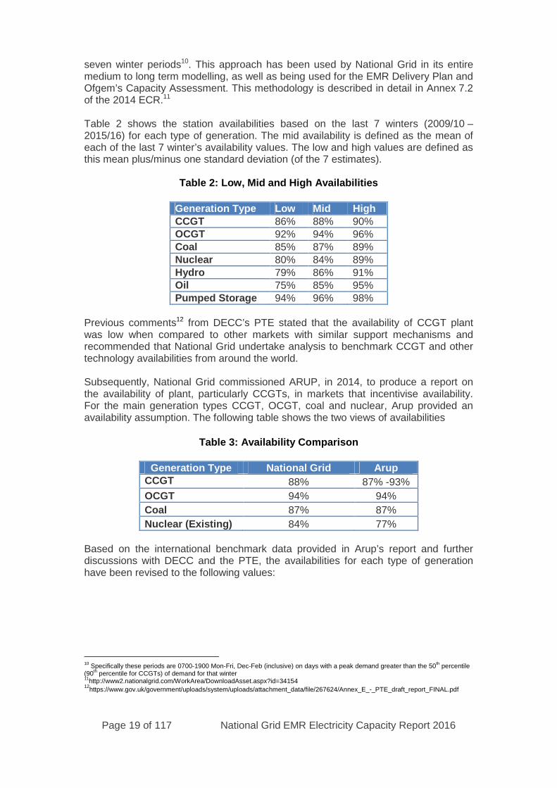
Table 2 shows the station availabilities based on the last 7 winters (2009/10 –2015/16) for each type of generation. The mid availability is defined as the mean ofeach of the last 7 winter’s availability values. The low and high values are defined asthis mean plus/minus one standard deviation (of the 7 estimates).
Table 2: Low, Mid and High Availabilities
Generation Type Low Mid HighCCGT 86% 88% 90%OCGT 92% 94% 96%Coal 85% 87% 89%Nuclear 80% 84% 89%Hydro 79% 86% 91%Oil 75% 85% 95%Pumped Storage 94% 96% 98%
Previous comments12 from DECC’s PTE stated that the availability of CCGT plantwas low when compared to other markets with similar support mechanisms andrecommended that National Grid undertake analysis to benchmark CCGT and othertechnology availabilities from around the world.
Subsequently, National Grid commissioned ARUP, in 2014, to produce a report onthe availability of plant, particularly CCGTs, in markets that incentivise availability.For the main generation types CCGT, OCGT, coal and nuclear, Arup provided anavailability assumption. The following table shows the two views of availabilities
Table 3: Availability Comparison
Generation Type National Grid ArupCCGT 88% 87% -93%
OCGT 94% 94%
Coal 87% 87%
Nuclear (Existing) 84% 77%
Based on the international benchmark data provided in Arup’s report and furtherdiscussions with DECC and the PTE, the availabilities for each type of generationhave been revised to the following values:
10 Specifically these periods are 0700-1900 Mon-Fri, Dec-Feb (inclusive) on days with a peak demand greater than the 50th percentile(90th percentile for CCGTs) of demand for that winter11
http://www2.nationalgrid.com/WorkArea/DownloadAsset.aspx?id=3415412
https://www.gov.uk/government/uploads/system/uploads/attachment_data/file/267624/Annex_E_-_PTE_draft_report_FINAL.pdf
Page 20 of 117 National Grid EMR Electricity Capacity Report 2016
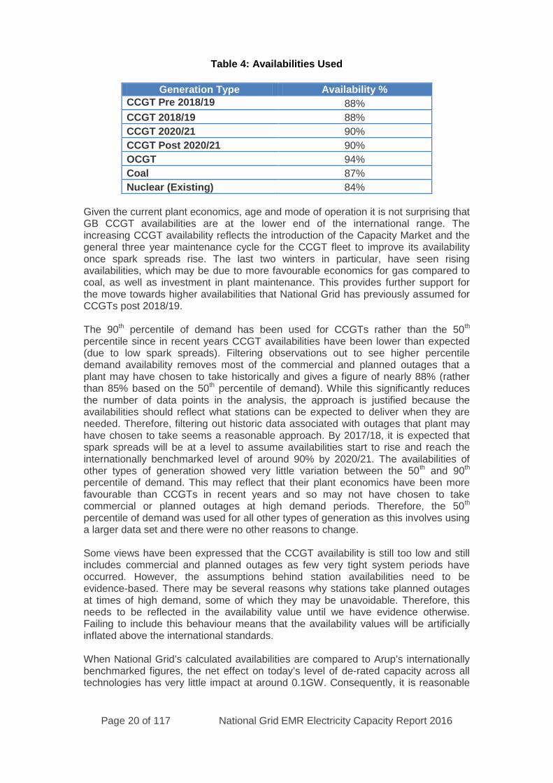
Table 4: Availabilities Used
Generation Type Availability %CCGT Pre 2018/19 88%
CCGT 2018/19 88%
CCGT 2020/21 90%
CCGT Post 2020/21 90%
OCGT 94%
Coal 87%
Nuclear (Existing) 84%
Given the current plant economics, age and mode of operation it is not surprising thatGB CCGT availabilities are at the lower end of the international range. Theincreasing CCGT availability reflects the introduction of the Capacity Market and thegeneral three year maintenance cycle for the CCGT fleet to improve its availabilityonce spark spreads rise. The last two winters in particular, have seen risingavailabilities, which may be due to more favourable economics for gas compared tocoal, as well as investment in plant maintenance. This provides further support forthe move towards higher availabilities that National Grid has previously assumed forCCGTs post 2018/19.
The 90th percentile of demand has been used for CCGTs rather than the 50th
percentile since in recent years CCGT availabilities have been lower than expected(due to low spark spreads). Filtering observations out to see higher percentiledemand availability removes most of the commercial and planned outages that aplant may have chosen to take historically and gives a figure of nearly 88% (ratherthan 85% based on the 50th percentile of demand). While this significantly reducesthe number of data points in the analysis, the approach is justified because theavailabilities should reflect what stations can be expected to deliver when they areneeded. Therefore, filtering out historic data associated with outages that plant mayhave chosen to take seems a reasonable approach. By 2017/18, it is expected thatspark spreads will be at a level to assume availabilities start to rise and reach theinternationally benchmarked level of around 90% by 2020/21. The availabilities ofother types of generation showed very little variation between the 50th and 90th
percentile of demand. This may reflect that their plant economics have been morefavourable than CCGTs in recent years and so may not have chosen to takecommercial or planned outages at high demand periods. Therefore, the 50th
percentile of demand was used for all other types of generation as this involves usinga larger data set and there were no other reasons to change.
Some views have been expressed that the CCGT availability is still too low and stillincludes commercial and planned outages as few very tight system periods haveoccurred. However, the assumptions behind station availabilities need to beevidence-based. There may be several reasons why stations take planned outagesat times of high demand, some of which they may be unavoidable. Therefore, thisneeds to be reflected in the availability value until we have evidence otherwise.Failing to include this behaviour means that the availability values will be artificiallyinflated above the international standards.
When National Grid’s calculated availabilities are compared to Arup’s internationallybenchmarked figures, the net effect on today’s level of de-rated capacity across alltechnologies has very little impact at around 0.1GW. Consequently, it is reasonable

Page 21 of 117 National Grid EMR Electricity Capacity Report 2016
to suggest that the two methods validate one another and the figures for GB areevidence-based, credible and auditable.
The nuclear availability from Arup was considered to be at the low end of the range.National Grid has gathered information from Grid Code obligations and stakeholderfeedback, not available to Arup, to inform the final discussion on nuclear availability.
National Grid has used the above approach to determine station availabilities for thelast few years. While informal consultations on the approach have been conductedthrough discussions at industry forums and bilateral meetings it is important that allstakeholders have an opportunity to engage in this process. This will help NationalGrid understand any concerns that stakeholders may have regarding this approachand help to inform any future changes to the methodology. Therefore, National Gridcontinues to welcome comments and questions on this approach either throughemail ([email protected]), industry forums or bilateral meetings.
During such consultations our assumptions of independence of generating units wasquestioned, in that the unavailability of one generating unit may be linked to theavailability of one or more other units. If some dependence is assumed, this could putdownward pressure on the availability figures. However, further detailed analysiswould need to be carried out in order to understand the implications of changing suchassumptions. This would require consultation with DECC and the PTE, with a view toundertaking a development project for next year.
Intermittent renewable plants run whenever they are able to, and so the availability ofthe fuel source is the most significant factor. When considering these plants, NationalGrid looks to their expected contribution to security of supply over the entire winterperiod. For wind, this is achieved by considering a history of wind speeds observedacross GB, feeding in to technology power curves, and running a number ofsimulations to determine its expected contribution. This concept is referred to asEquivalent Firm Capacity (EFC). In effect, it is the level of 100% reliable (firm) plantthat could replace the entire wind fleet and contribute the same to security of supply.The wind EFC depends on any factors that affect the distribution of available windgeneration. These include: the amount of wind capacity installed on the system;where it’s located around the country; and the amount of wind generation that mightbe expected at periods of high demand. It also depends on how tight the system. Asthe system gets tighter, the wind EFC increases for the same level of installedcapacity as there are more periods when wind generation is needed to meet demandrather than displacing other types of generation in the merit order. It should be notedthat the EFC is not an assumption of wind output at peak times and consequentlyshould not be considered as such.
In the DDM for years apart from 2018/19, we have modelled the contribution ofinterconnectors at peak times by assigning a probabilistic distribution to eachinterconnector, defining the probability of each import / export level for a given levelof net system margin. These distributions were derived from the analysis carried outby Baringa (see Chapter 4). The DDM calculated an EFC for interconnection whichwas used as an estimate of the aggregate interconnector de-rated capacity. Note thatthe modelled de-rating factor for interconnection has no impact on the total de-ratedcapacity (including interconnection), required to meet the Reliability Standard. In theauction, interconnection capacity will compete with other types of new/existingeligible capacity to meet the capacity requirement.
Page 22 of 117 National Grid EMR Electricity Capacity Report 2016
Given that the recommended capacity to secure is a de-rated value, the assumptionsaround availability of both conventional and renewable capacity have limited impacton the recommendation. Broadly the same level of de-rated capacity is required to hitthe 3 hours LOLE; however, the name-plate capacity required to achieve that level ofde-rated capacity will be slightly different. See Chapter 5, 6 & 7 for the details for thedetails of how de-rated capacity changes with variations in availability assumptions.
2.4 DDM Outputs Used in the ECR
For the purpose of the ECR, the key outputs utilised from the DDM for each yearmodelled from 2017/18 to 2030/31 are the aggregate capacity values, specifically:
A. Total de-rated capacity required to hit 3 hours LOLEB. De-rated capacity to secure in the Capacity Market auctionC. De-rated non-eligible capacity expected to be delivered outside the Capacity
Market auctionD. Total nameplate capacity split by CM and non-CM eligible technologies.E. De-rated capacity already contracted for, from previous auctions
Note that A = B + C. Further details on the modelling and aggregate capacities canbe found in Annex.
In addition to the aggregate capacity values, for the purpose of calculating therecommended capacity to secure in 2017/18, 2018/19 and 2020/21, the ECR alsoutilises the expected energy unserved (EEU) values for potential de-rated capacitylevels in all three years (see Chapters 5, 6 & 7 for more details).
No other outputs from the DDM are utilised directly in the ECR.
2.5 PTE Recommendations
In the PTE’s “Final Report on National Grid’s Electricity Capacity Report” – June201513 they identified a number key issues, themes and recommendations whichNational Grid agree need further investigation and have therefore undertaken anumber of development projects as part of this year’s process:
Additional analysis should be undertaken to understand the potentialcontribution from DSR and distribution connected generation(Recommendation 11):
As part of the 2016 FES process we have carried out extensive searchesacross a range of sources to obtain a more accurate figure for the levels ofinstalled distribution connected generation. This has provided detailedcapacity figures for all technologies but unfortunately not their levels ofgeneration. We are currently in negotiation with ElectraLink (a commercialcompany owned by a group of Distribution Network Operators (DNOs)) tosecure half hourly data for the last few years for each distribution connectedplant. This data should provide insight into how patterns of generation havechanged over the recent past as financial incentives have improved andshould deliver the increased knowledge and understanding the PTE sought.This latter point will address the follow up to the PTE’s Recommendation 10
13https://www.gov.uk/government/uploads/system/uploads/attachment_data/file/438714/PTE_2015_ECR_Report_final.pdf
Page 23 of 117 National Grid EMR Electricity Capacity Report 2016
from their 2014 report which requested more analysis on distributedgeneration availabilities.
National Grid has been working closely with industry via its PowerResponsive campaign to help inform and facilitate greater participation in bothtrue DSR (i.e. demand shifting or demand reduction) and distributedgeneration. This campaign has included extensive engagement, industryworkshops and published documents all highlighting the financial incentivesand ways to participate. This campaign appears to have successfullycontributed to the increased participation of both DSR and distributedgeneration seen in the market during 2015/16.
The PTE expressed concerns over the inclusion of extreme weather eventsas sensitivities within the LWR process as the LOLE calculation alreadyallows for such events and therefore there was a danger of double counting.
To help address this concern we commissioned academic consultants fromDurham University and Heriot Watt University (Zachary, Wilson & Dent) toinvestigate the statistical uncertainty around the non-linearity of impact onLOLE. This work centred on the fact that while LOLE is a long run averagemetric, it was only the most extreme observations that make made anysignificant contribution to it and hence uncertainty associated with theseestimates was crucial to understanding uncertainty as a whole. For example,a major source of uncertainty in statistical analysis results from the dramaticeffects of varying winter severity. It is far from clear that the probability of asevere winter in a future year under study is well approximated by the fractionof severe winters in the historical data (10 years), and for this reason alone itmakes sense to also report estimates of LOLE, etc., conditional on winterseverity (as it standard practice in many other countries). The academic workconcluded that this is not a case of double counting.
Consequently, it is fair to say that the PTE’s comments are valid when using along series of historical data (note for average weather conditions the METOffice uses 30 years of data); however, as we are only using 10 years it istherefore not long enough to say with any certainty (without some furtherdetailed analysis which could be addressed by a development project for nextyear) that it is representative of future years being studied. Hence weproposed to DECC and the PTE that we need to address this uncertainty inweather by including a cold weather sensitivity based on a recent non-extreme cold winter e.g. 2010/11. Given the supporting evidence of thisacademic research the PTE agreed to the inclusion of the cold and warmweather sensitivities in the 2016 analysis. Note that we wouldn’t considerusing a long series of demand as that wouldn’t be representative of demandin future years as the make-up of demand was considerably different 20 yearsago e.g. manufacturing versus service industries.
National Grid should expand its analysis of loss of load events to takeaccount of the volume, frequency, duration, forewarning and predictability ofloss of load events (Recommendation 12):
This recommendation can be addressed in two parts; the modelling of loss ofload events (for which in the past we have undertaken some work for Ofgem)and the details around emergency procedures that would be utilised leadingup to controlled disconnections by the DNOs.
Page 24 of 117 National Grid EMR Electricity Capacity Report 2016
The functionality of the DDM version currently utilised for the Capacity Marketwork doesn’t produce information on frequency and duration as it is timecollapsed rather than sequential. While a module of DDM has a sequentialcapability there are limited reliable data sources currently available to enablethe model to be effectively run. Also the run time of any sequential modelwould need to be carefully considered due to the practicality of delivering theanalysis given the limited time available to undertake and deliver the work.However, we have run our own time collapsed Capacity Assessment model ina way that enables an approximation of frequency and duration metrics to becalculated. When we shared this analysis with DECC and the PTE they feltthat while interesting the frequency metrics could be misinterpreted, asverification required sequential modelling, and as it doesn’t impact theresulting capacity to secure figure, we agreed not to re-produce the analysisin our report.
The PTE have presented work undertaken by Imperial College London thatmodelled the GB market sequentially using a range of data including aInstitute of Electrical & Electronic Engineers (IEEE) dataset to producefrequency and duration statistics. This work provided interesting insight in tothe potential shape of loss of load events under a 3 hour loss of loadexpectation Reliability Standard. Any future development projects will centreon how these findings could be potentially translated into running the DDM ina practical way and ensure appropriate model run times to enable timelydelivery of outputs. Consequently, we would be happy to work with the PTEand DECC to agree a development project for the autumn to review anypotential options.
To address the second part; in addition to providing information on themitigating actions the System Operator can take we also provided a summaryof the Demand Control operating code, Demand Control decision andcommunication process, Demand Control instruction formats, data on the lastoccasions when it was utilised, data on historical Notification of InadequateSupply Margin (NISMs) and an overall summary. The PTE also wereinterested in understanding the process by which DNOs disconnectconsumers which unfortunately we were unable to provide as that issomething each DNO will undertake (potentially using different approacheswhich best suit their particular network), not National Grid.
While all the above information is important, it has no effect on our capacityrequirement recommendation as that is measured before any mitigating oremergency actions are taken. There are two practical reasons for this; firstly,these actions aren’t firm and therefore can’t be guaranteed and secondly,these are emergency actions and shouldn’t be planned to be utilisedotherwise they are no longer emergency actions. Note all ancillary servicecontracts we have are assumed to be utilised in the calculation to meet theReliability Standard with these mitigating and emergency actions being on topof those.
Concerns over the value of lost load (VoLL) being utilised in the LWRcalculation not reflecting the lower cost of mitigating actions and thereforedistorting the calculation with a potential for securing too much capacity.
Page 25 of 117 National Grid EMR Electricity Capacity Report 2016
There are two aspects to consider around these concerns; firstly, the processby which VoLL was estimated and secondly, the wider context around howVoLL is used within the Reliability Standard.
We agree with the PTE that in reality the VoLL would start lower than thefigure used for the LWR analysis of £17,000/MWh as mitigating actions aretaken, e.g. voltage reduction, but would then progressively increase as furtheractions are taken before rises above £17,000/MWh, as loads aredisconnected. Consequently, when London Economics estimated theaverage VoLL they took account of the increasing cost of differentcomponents of VoLL at the level of customer disconnections. There isinherent uncertainty in setting the level of VoLL and it is dependent on thequestions asked of consumers and whether the wider economic impacts areconsidered. The determination of VoLL is currently outside the scope of thisanalysis.
The other metric utilised within the LWR calculation is the Cost of New Entry(CONE) which is also based on an average figure when in reality it would alsohave a cost/supply curve. Consequently, adjustments in VoLL cannot beconsidered in isolation without considering CONE. As a development projectwe asked our academic consultants from Durham University and Heriot WattUniversity (Zachary, Wilson & Dent) to review the LWR process and one oftheir conclusions was that the ratio of VoLL to CONE would need to remainconsistent with that used when defining the Reliability Standard (i.e. ratio ofclose to 3 (£47/kW/yr / £17,000/MWh). This means that if VoLL was reducedthen CONE would also need to be reduced to maintain the same ratiootherwise the analysis would be basing its calculations on a differentReliability Standard.
In addition to enable the LWR decision tool to run effectively we need a singlevalue for both VoLL and CONE. To try and use cost/supply curves that varythese values would prove difficult to implement as it would make thecalculation extremely complex but more importantly would have no impact onthe recommended capacity to secure as the ratio of the two would alwaysneed to be 3.
DECC undertook some analysis in this area and as a result of the academicresearch outlined above, concluded that any review of VoLL would need toalign with the review of the Reliability Standard to be undertaken which willconsider a more sophisticated representation of both VoLL and CONE.
Develop a pan-European dispatch model with the functionality to simulate thebehaviour of interconnectors in a variety of market coupled scenarios(Recommendation 13):
To support our interconnector modelling for FES and EMR we commissionedBaringa to undertake analysis of annual and peak flows acrossinterconnectors utilising their Plexos pan-European model with flows beingdetermined predominantly by the relativity of generation short run marginalcosts (SRMCs) in each country. This modelling was enhanced from that usedlast year by the inclusion of scarcity premia, number of historical years utilisedand a larger number of simulations. More detail on this can be found inChapter 4.
Page 26 of 117 National Grid EMR Electricity Capacity Report 2016
For our FES and EMR analysis in 2017 and to support our role in IntegratedTransmission Planning & Regulation (ITPR) we have procured a pan-European market and network model from Pöyry which will enable us to runEuropean demand and generation scenarios in a similar way to those run forGB with dispatch based on relative SRMCs.
Further work should be carried out on the methodologies to select a singlede-rating factor for each interconnected system (Recommendation 14) andin choosing these factors DECC should err on the high side(Recommendation 15):
Our report provides advice to DECC on the range of potential de-ratingfactors that could be used for each interconnected country. This analysis isbased on work from a range of consultants as well our own analysis ofweather and the benefits from connected systems. However, due to aperceived conflict of interest with our Business Development subsidiary thatowns and operates interconnectors it was determined to be inappropriate forus to recommend any de-rating factors for any individual existing or proposedinterconnectors. With regard to the ranges we provide for interconnectedsystems and countries we have taken on board these comments whendeveloping the higher end of the range for this year’s report.
Consequently, DECC with the support of the PTE undertook the analysis toproduce each interconnector de-rating factor last year, with input from uswhen requested. This means we are unable to comment on how theserecommendations will be addressed this year but are happy to support DECCin their analysis.
One recommendation from their 2014 report (Recommendation 2) which thePTE felt hadn’t been fully addressed last year related to the use of the relativelikelihood of scenarios and sensitivities used within the LWR decision tool. Inparticular they referred to the inclusion of the extreme weather eventssensitivities.
As part of last year’s analysis we undertook a series of stress tests of theLWR approach that considered various levels of probabilities or weightingsbeing applied to different sensitivities. All scenarios and sensitivities that wereincluded had to be credible and based on real examples, as with this year’smethodology. Notwithstanding the imprecise nature of assigning probabilitiesto most scenarios and sensitivities, the analysis found that to change theoutcome of the LWR required very low probabilities to be used which meantthey would need to be non-credible sensitivities and therefore wouldn’t havebeen included anyway. Academic analysis from our academics from DurhamUniversity and Heriot Watt University (Zachary, Wilson & Dent) supported thisconclusion; however, this work also suggested considering as part of anyfuture development work the potential use of a Bayesian approach14.Consequently, we will investigate this as a development project for nextyear’s analysis.
To provide some practical insight to the potential application of assigningprobabilities to sensitivities a recent example highlights the difficulty
14Bayesian analysis is a statistical procedure which endeavours to estimate parameters of an underlying distribution based on an
assessment of the observed relative likelihoods.
Page 27 of 117 National Grid EMR Electricity Capacity Report 2016
associated with such an exercise. When we were carrying out analysis on thecapacity to procure through the Contingency Balancing Reserve products for2016/17 we incorporated coal closure sensitivities up to 2.8GW within theLWR tool (similar to the non-delivery sensitivities used in this report). At thetime it was suggested that we should assign probabilities but it was decidedagainst it given the challenging economic climate for coal stations andfeedback from the station operators. This proved to be the correct actionbecause within a short time of that analysis two coal stations announcedclosure in line with that sensitivity. This reinforces the arbitrary nature ofassigning probabilities or weightings to credible sensitivities as they can in avery short timeframe be proved incorrect.
With regard to the inclusion of the extreme weather sensitivities which, intheory, can be apportioned a probability; firstly, we have addressed the PTE’sconcerns over their inclusion in our analysis in the response to the secondbullet above and secondly, their position within the previous ECR’s range ofpotential capacity requirements prevents them from affecting the outcome asthe sensitivities at the ends of the range determine the outcome of any LWRcalculation. Consequently, while providing important information that enablesnon-statisticians to assess risk unless these sensitivities are at the end of thepotential range of credible outcomes they don’t affect the recommendedcapacity to secure.
In conclusion National Grid is confident it has addressed, where possible, all thePTE’s concerns within the approach being used for the 2016 ECR.
2.6 Modelling Enhancements since Last Report
Section 2.5 describes a number of development projects carried out in response tothe PTE’s 2015 final report. In addition to these projects we have, in consultation withDECC, carried out or commissioned a number of modelling development projects toinform and improve the process. These projects include a review of the LWRmethodology, research on the non-linear nature of LOLE, enhancements to the DDM,an update to the interconnector modelling analysis, the calculation of an offshorepower curve and updated analysis to assess the relationship between windgeneration and demand at times of cold weather.
Following the completion of these development projects, a number of recommendedchanges were agreed with DECC and the PTE and incorporated into this year’s ECRmodelling. These recommendations can be split into three categories:
Data input assumptions Modelling changes Interpretation of LWR results
2.6.1 Data Input Assumptions
The main enhancements to the input data used by the DDM relate to the inclusion ofa separate wind stream for offshore wind derived from a new offshore wind powercurve, enhancements to the modelling of interconnector distributions and a widerrange of credible sensitivities as described below.
Page 28 of 117 National Grid EMR Electricity Capacity Report 2016
Offshore Wind Power Curve
Previously the DDM used a single wind stream (time series of historic hourly windload factors) derived from an onshore wind power curve as there was no reliable dataavailable to derive a separate offshore wind turbine power curve.
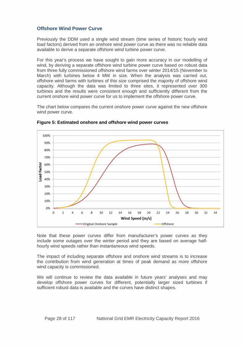
For this year’s process we have sought to gain more accuracy in our modelling ofwind, by deriving a separate offshore wind turbine power curve based on robust datafrom three fully commissioned offshore wind farms over winter 2014/15 (November toMarch) with turbines below 4 MW in size. When the analysis was carried out,offshore wind farms with turbines of this size comprised the majority of offshore windcapacity. Although the data was limited to three sites, it represented over 300turbines and the results were consistent enough and sufficiently different from thecurrent onshore wind power curve for us to implement the offshore power curve.
The chart below compares the current onshore power curve against the new offshorewind power curve.
Figure 5: Estimated onshore and offshore wind power curves
Note that these power curves differ from manufacturer’s power curves as theyinclude some outages over the winter period and they are based on average half-hourly wind speeds rather than instantaneous wind speeds.
The impact of including separate offshore and onshore wind streams is to increasethe contribution from wind generation at times of peak demand as more offshorewind capacity is commissioned.
We will continue to review the data available in future years’ analyses and maydevelop offshore power curves for different, potentially larger sized turbines ifsufficient robust data is available and the curves have distinct shapes.
Page 29 of 117 National Grid EMR Electricity Capacity Report 2016
Enhanced interconnector modelling
Baringa has updated and enhanced its interconnector modelling for this year’s ECR(see section 4.3 for more details). This analysis was used to create probabilisticinterconnector distributions for each country used in the 2017/18 and 2020/21 modelruns. For the 2018/19 runs, where interconnectors have been excluded from theCapacity Market, we have assumed a static peak flow that is consistent with the de-rating factors used in 2019/20 and a range of sensitivities similar to those used in theContingency Balancing Reserve (CBR) analysis.
A wider range of credible sensitivities
Academic work on LWR highlighted that effort should be concentrated on thesensitivities at the extreme ends of the range as these largely drive the outcome fromthe LWR calculation tool. In consultation with DECC and the PTE we have expandedthe range of credible sensitivities modelled in this year’s ECR to give a range for2017/18 that is similar to those used in the CBR analysis (see Chapter 3 for furtherdetails on the sensitivities modelled)
2.6.2 Modelling Changes
The main enhancements to the modelling relates to the DDM upgrades and analysisand improvements in the modelling of the relationship between wind generation anddemand at times of cold weather.
DDM Upgrades and Analysis
National Grid commissioned Lane, Clark & Peacock (LCP) to carry out upgrades tothe DDM and to carry out analysis on some of its outputs.
One key DDM upgrade focused on the modelling of T-1 auctions. Previously theDDM simulated the (T-4) CM auction to secure the capacity required for eachdelivery year. This upgrade extended the functionality for years where the results of aT-4 auction are known, whereby simulating the T-1 auction secures any additionalcapacity required above the contracted capacity assumed in the modelling. For thisupgrade the DDM calculates the previously contracted capacity using the modelledcapacity of contracted plants assumed to be operational – this may be different fromthe actual contracted capacity awarded in the T-4 auction e.g. if the plant wasassumed to close in the scenario modelled or if the modelled capacity value (basedon Transmission Entry Capacity (TEC)) is different to the connection capacitydeclared in the T-4 auction.
Another key upgrade provided functionality to allow for a variable level of correlationbetween wind output and demand to be modelled in line with the recommendationfrom academic research (see Chapter 3). In addition some outputs were added toimprove the reporting of de-rated capacity and to enable the impacts of capacitychanges on LOLE and EEU to be assessed without rerunning the model.
LCP also carried out analysis that confirmed that the DDM and National Grid’s ownprobabilistic capacity adequacy model (used to determine the requirement for CBR)will produce consistent metrics (e.g. LOLE) when given exactly the same(transmission level) inputs. In addition, the analysis showed there was a smalldifference in LOLE when modelling at a GB end-consumer level (as per the analysis
Page 30 of 117 National Grid EMR Electricity Capacity Report 2016
carried out for the Electricity Capacity Report) compared to a transmission level (asper the CBR analysis), but these differences were within the 95% confidence intervalof the LOLE calculation.
Note that in our modelling, we did not include attempt to quantify any whole systemcosts impacts as these do not directly determine the de-rated capacity required tomeet the Reliability Standard.
Relationship between Wind Generation and Demand
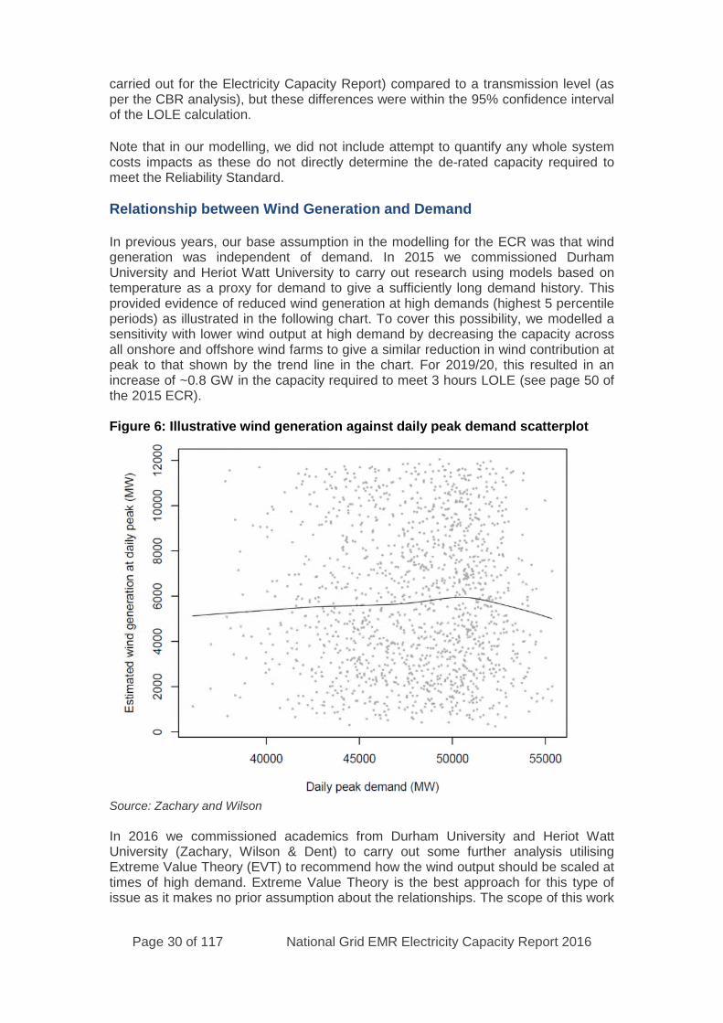
In previous years, our base assumption in the modelling for the ECR was that windgeneration was independent of demand. In 2015 we commissioned DurhamUniversity and Heriot Watt University to carry out research using models based ontemperature as a proxy for demand to give a sufficiently long demand history. Thisprovided evidence of reduced wind generation at high demands (highest 5 percentileperiods) as illustrated in the following chart. To cover this possibility, we modelled asensitivity with lower wind output at high demand by decreasing the capacity acrossall onshore and offshore wind farms to give a similar reduction in wind contribution atpeak to that shown by the trend line in the chart. For 2019/20, this resulted in anincrease of ~0.8 GW in the capacity required to meet 3 hours LOLE (see page 50 ofthe 2015 ECR).
Figure 6: Illustrative wind generation against daily peak demand scatterplot
Source: Zachary and Wilson
In 2016 we commissioned academics from Durham University and Heriot WattUniversity (Zachary, Wilson & Dent) to carry out some further analysis utilisingExtreme Value Theory (EVT) to recommend how the wind output should be scaled attimes of high demand. Extreme Value Theory is the best approach for this type ofissue as it makes no prior assumption about the relationships. The scope of this work

Page 31 of 117 National Grid EMR Electricity Capacity Report 2016
was shaped by discussions with the PTE and the recommendations were acceptedand agreed by the PTE.
This analysis was based on the last 10 years of winter (Nov-Mar) data as that is allthe paired wind and demand data that is available. The EVT analysis shows thatwind output does fall at times of high demand as shown by an increase in the LOLEcompared to the assumption of independence. The EVT approach modelled yearsindividually and averaged the results from the individual years whereas the previousmethodology used pooled (10 year) demand and (36 year) wind data15.
The longer-term recommendation of the research was to consider modelling eachyear separately, but that is not currently possible within DDM and would require adevelopment project for implementation in 2017 or later. However, functionality doesnow exist within DDM to use a scaling factor to reduce the wind output at times ofhigh daily peak demand to give results consistent with the EVT approach (seeChapter 3). For the 2016 ECR, the research recommended scaling wind outputbased on a 10 years pooled (Nov-Mar) wind history to give LOLE figures equivalentto the EVT approach. This results in a scaling of 0.9 (i.e. wind output is reducedlinearly from 100% to 90% for daily peak demands between the thresholds of 92%and 102% of ACS peak demand).
The research also suggested that a range for wind output at times of peak demandcould be obtained by assuming independence of wind and demand (the previousbase assumption) at one end and at the other a higher scaling than used for the basecase of 0.8 compared to 0.9. This range formed the basis of the high and low windsensitivities (See Chapter 3).
2.6.3 Interpretation of Results
Demand is a key element in the decision around the level of capacity to secure in theCM auctions along with the level of non-CM capacity assumed connected in the yearin question. To enable the most cost efficient level of capacity to be secured NationalGrid and Ofgem agreed the DFA Incentive covering demand forecasts that benefitsboth the consumer and National Grid (similar to the Balancing & Services IncentiveScheme (BSIS) scheme for operating the network)
In agreement with Ofgem, due to the impact of greater uncertainty in the deploymentaround non-CM eligible generation the decision was made not to develop anincentive around that metric.
The DFA Incentive applies to the demands associated with the scenario or sensitivitythat sets the recommendation on the capacity to secure in future capacity auctions.Hence the recommendation needs to be based on a scenario or sensitivity that usesour Base Case (produced specifically for DFA Incentive) and not some other FESscenario demand.
For this reason we have applied the sensitivities to the Base Case (see Chapter 3).We have also modelled a greater number of sensitivities to improve the granularity ofpotential capacity to secure values so that the gap between values is ideally no morethan the confidence interval of the calculation (±400 MW). Note all capacity to secure
15Previously 10 years of winter period demand values were pooled to create a single demand distribution and 36 years of winter
period wind speeds were used to create a single pooled wind distribution

Page 32 of 117 National Grid EMR Electricity Capacity Report 2016
figures in this report are quoted to the nearest 0.1 GW (100 MW), given the size ofthe 95% confidence interval as + or – 400 MW.
The model run results from the Base Case and sensitivities along with the four FESscenarios was input into the LWR decision tool which selects a volume (consistentwith one of the scenarios or sensitivities) to recommend for the year in question. Themost likely outcome, as sensitivities are based around the Base Case i.e. DFAIncentive level of demand, is that the LWR tool selects one of these sensitivities.However, it is still possible the LWR tool could select a FES scenario with a differentdemand and thus an adjustment would be required e.g. as per Chapter 6 for2020/21.
Given the inherent uncertainty in the calculation for the capacity requirement for eachdefined scenario or sensitivity, (as illustrated by a 95% confidence interval) the realanswer could be anywhere within that range. Hence any movement away from theLWR output is statistically valid so long as it remains within this range. In the eventthat the capacity requirement associated with a FES scenario is chosen by the LWRtool then a small adjustment would be required to bring it into line with the DFAIncentive. This would manifest itself as a small movement away from the LWRanswer to the nearest sensitivity that was based on the Base Case demandsproduced specifically for the DFA Incentive. This adjustment would be within theconfidence interval i.e. less than ±400 MW and therefore would be statisticallypermissible. See Chapter 6 for an example of where this adjustment has been used.
2.7 Quality Assurance
When undertaking any analysis National Grid looks to ensure that a robust QualityAssurance (QA) process has been implemented. National Grid has previouslyworked closely with DECC’s Modelling Integrity team to ensure that the QA processclosely aligned to DECC’s in house QA process.
The QA checks below are focussed on the points in the process where data istransferred from one model, or system, to another, together with the model outputs.These are:
1. Interconnector flows – Check the interconnector flowassumption/distribution
2. Scenario inputs – Check the model input assumptions3. Parameter Inputs / CM Results/ Historic Demand inc. distributed wind –
Check the model setup assumptions4. Scenarios to DDM Translation – Check the input from the FES process into
the DDM model5. DDM Outputs - Check model outputs are consistent with inputs and scenario
criteria6. Capacity to Secure Process – Check the inputs and outputs used to
determine a range and recommended capacity to secure
The process is overseen by the PTE and they review and report on the overallprocess. Internally the process has governance under Director UK SystemOperation. National Grid has also worked closely with LCP to check and verify theresults obtained as part this analysis to reinforce the robustness of the QA process.For details of the QA undertaken by National Grid see the Annex.
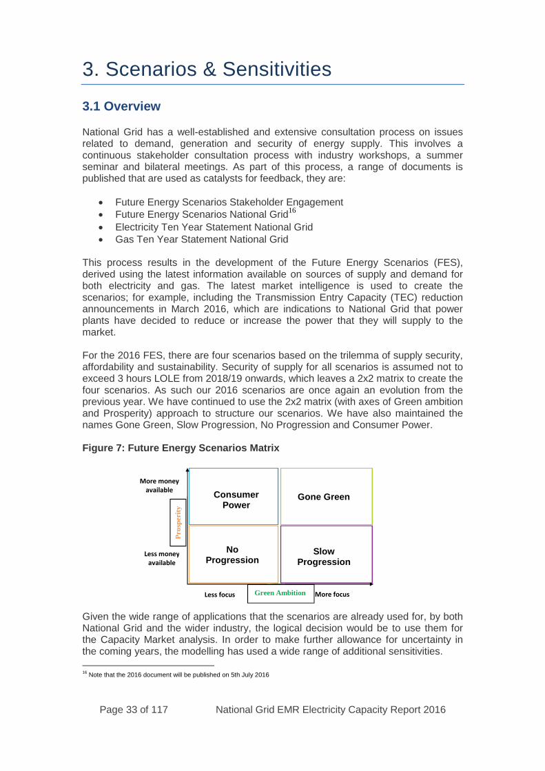
Page 33 of 117 National Grid EMR Electricity Capacity Report 2016
3. Scenarios & Sensitivities
3.1 Overview
National Grid has a well-established and extensive consultation process on issuesrelated to demand, generation and security of energy supply. This involves acontinuous stakeholder consultation process with industry workshops, a summerseminar and bilateral meetings. As part of this process, a range of documents ispublished that are used as catalysts for feedback, they are:
Future Energy Scenarios Stakeholder Engagement Future Energy Scenarios National Grid
16
Electricity Ten Year Statement National Grid Gas Ten Year Statement National Grid
This process results in the development of the Future Energy Scenarios (FES),derived using the latest information available on sources of supply and demand forboth electricity and gas. The latest market intelligence is used to create thescenarios; for example, including the Transmission Entry Capacity (TEC) reductionannouncements in March 2016, which are indications to National Grid that powerplants have decided to reduce or increase the power that they will supply to themarket.
For the 2016 FES, there are four scenarios based on the trilemma of supply security,affordability and sustainability. Security of supply for all scenarios is assumed not toexceed 3 hours LOLE from 2018/19 onwards, which leaves a 2x2 matrix to create thefour scenarios. As such our 2016 scenarios are once again an evolution from theprevious year. We have continued to use the 2x2 matrix (with axes of Green ambitionand Prosperity) approach to structure our scenarios. We have also maintained thenames Gone Green, Slow Progression, No Progression and Consumer Power.
Figure 7: Future Energy Scenarios Matrix
Given the wide range of applications that the scenarios are already used for, by bothNational Grid and the wider industry, the logical decision would be to use them forthe Capacity Market analysis. In order to make further allowance for uncertainty inthe coming years, the modelling has used a wide range of additional sensitivities.
16Note that the 2016 document will be published on 5th July 2016
More moneyavailable
Less moneyavailable
More focus
Gone GreenConsumerPower
SlowProgression
NoProgression
Less focus Green Ambition
Pro
sper
ity

Page 34 of 117 National Grid EMR Electricity Capacity Report 2016
For the purposes of modelling scenarios for the Capacity Market DECC’s DDMmodel has been used, as described in Chapter 2. Thus while the non-CapacityMarket technologies are fixed to the levels assumed in each of the FES scenarios,DDM calculates Capacity Market (CM) qualified capacity to ensure that the 3 hoursLOLE Reliability Standard is met. Hence over time the capacities shown in thisanalysis may diverge from those in the original FES scenarios.
Base Case
In addition to the four FES scenarios and to be compliant with the new DFA Incentiveagreed with Ofgem we have developed a new Base Case from which all thesensitivities will be run from. This Base Case follows exactly the same principlesusing the same modelling approach as the FES scenarios to give a 5 year demandand generation background that is within the four FES scenarios range. Due to theinherent uncertainty across the market beyond 2020/21 the Base Case then followsthe FES scenario that is closest to its DFA Incentive demand level in 2020/21thereafter, which for the 2016 FES is Slow Progression.
The Base Case assumes some closure or delay in CM contracted plant over the nextfive years due to, in particular, the challenging economic climate for coal stationoperators.
3.2 Scenario Descriptions
Descriptions of the four FES scenarios (for GB) are detailed below with a high levelsummary of the resulting capacity technology split between CM and non-CM plantfollowing the DDM runs shown in the Annex. While DDM generates the final capacityfigures required to meet the Reliability Standard for each scenario and sensitivity theFES scenarios are key inputs in determining the capacity to secure as they set thelevel of non-CM capacity which DDM then works around which explains the need todescribe the assumptions behind each scenario.
3.2.1 Gone Green
Gone Green is a world where policy intervention and innovation are both ambitiousand effective in reducing greenhouse gas emissions. The focus on long-termenvironmental goals, high level of prosperity and advanced European harmonisationensure that the 2050 carbon reduction target is achieved.
Demand
Policy and innovation is focused on energy efficiency across the residential, industrialand commercial sectors, due to greater political certainty over Green Ambitions. Non-binding policies such as EU’s 2030 Climate & Energy Framework, which seeks anappliance energy saving of 30%, are adopted. From 2020 carbon reduction policyfocuses more on the electrification of heating across all the three sectors.Technological innovation and a high level of prosperity leads to a high take up ofelectric vehicles. These all combine to initially reduce demand in the short term andthen to increase demand from the mid 2020s.
Page 35 of 117 National Grid EMR Electricity Capacity Report 2016
Generation
There is advanced innovation in green technologies with particular emphasis onrenewable generation. Sources of renewable generation include solar PV, wind andmarine. The sustained focus on environmental targets and favourable economicconditions, ensures continued support for the deployment of renewable and lowcarbon technologies with significant levels of Carbon Capture and Storage (CCS),renewable generation and nuclear into the future. EU aspirations regardinginterconnector capacity for each Member State remain applicable.
3.2.2 Slow Progression
Slow Progression is a world where economic conditions limit society’s ability totransition as quickly as desired to a renewable, low carbon world. Choices forresidential consumers and businesses are restricted, yet a range of new technologiesand policies do develop. This results in some progress towards decarbonisation butat a slower pace than society would like.
Demand
Policy is focused on energy efficiency, due to greater political certainty over levels ofGreen Ambition but efforts are constrained due to less prosperity, as such the EU’s2030 Climate & Energy Framework is less ambitious. Lower economic growth furtherhastens industrial demand decline. Both commercial demand and residentialdemand slowly increase due to an increasing population and slower uptake of energyefficiency measures. These all combine to leave demand remaining flat until around2030 after which there is a slight increase and demand returns to today’s level, by2040.
Generation
The sustainability agenda ensures that the generation landscape is dominated byrenewable technology. Ambition for innovation is constrained by financial limitations,which, in comparison to Gone Green, leads to a slower uptake of renewables.
3.2.3 No Progression
No Progression is a world where business as usual activities prevail. Society isfocused on the short term, concentrating on security of supply and affordability abovegreen ambition. Traditional sources of gas and electricity dominate the supply marketand there is little innovation altering how energy is used.
Demand
There is less political focus on energy efficiency due to political uncertainty overlevels of Green Ambition. Lower economic growth hastens industrial demand decline.Commercial demand slowly declines, as the relative cost of energy favours gas overelectric heating. Residential demand slowly increases due to an increasingpopulation and slower uptake of energy efficiency measures. These all combine toleave peak demand remaining flat until the early 2030’s after which there is a slowrise as the residential demand picks up.
Page 36 of 117 National Grid EMR Electricity Capacity Report 2016
Generation
There is less money available for innovation and so there are only incrementalimprovements in existing technology. Gas and existing coal feature in the generationmix over renewables and nuclear, with focus being on the cheapest sources ofenergy. The lack of focus on the green agenda and limited financial supportavailable for low carbon technologies results in a limited new build programme fornuclear and minimal deployment of less established technology e.g. CCS andmarine.
3.2.4 Consumer Power
Consumer Power is a market-driven world, with limited government intervention. Highlevels of prosperity allow for high investment and innovation. New technologies areprevalent and focus on the desires of consumers over and above reducinggreenhouse gas emissions.
Demand
Higher economic growth leads to increasing levels of innovation across the sectors,in particular being driven by consumers in the residential sector, including a stronguptake of electric vehicles. Policy is focused on energy efficiency, but efforts areconstrained by political uncertainty over levels of Green Ambition. Industry continuesto decline over the period. Commercial demand declines, as the relative cost ofenergy favours gas over electric heating, but it flattens off in the mid-2020s. Theseall combine to increase demand over the period
Generation
The favourable economic conditions encourage development of generation at alllevels. There is high renewable generation at a local level and high volumes ofnuclear and gas generation at a national level. There is minimal deployment of newlow carbon technologies, with these technologies not achieving commercial scaleoperation e.g. CCS and marine.
3.3 Demand Forecast until 2020/21
The demand forecast until 2020/21 has been created for the five year period 2016/17to 2020/21. It supports the DFA Incentive which is instrumental in recommending acapacity to secure. This forecast is based on a central economic view, current energypolicies, limited consumer behaviour change and the uptake of new technologies -such as electric vehicles and heat pumps.
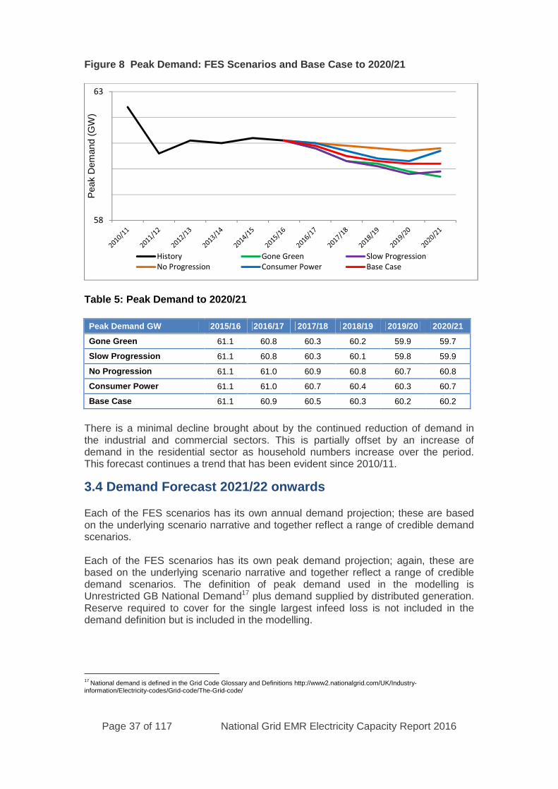
Page 37 of 117 National Grid EMR Electricity Capacity Report 2016
Figure 8 Peak Demand: FES Scenarios and Base Case to 2020/21
Table 5: Peak Demand to 2020/21
Peak Demand GW 2015/16 2016/17 2017/18 2018/19 2019/20 2020/21
Gone Green 61.1 60.8 60.3 60.2 59.9 59.7
Slow Progression 61.1 60.8 60.3 60.1 59.8 59.9
No Progression 61.1 61.0 60.9 60.8 60.7 60.8
Consumer Power 61.1 61.0 60.7 60.4 60.3 60.7
Base Case 61.1 60.9 60.5 60.3 60.2 60.2
There is a minimal decline brought about by the continued reduction of demand inthe industrial and commercial sectors. This is partially offset by an increase ofdemand in the residential sector as household numbers increase over the period.This forecast continues a trend that has been evident since 2010/11.
3.4 Demand Forecast 2021/22 onwards
Each of the FES scenarios has its own annual demand projection; these are basedon the underlying scenario narrative and together reflect a range of credible demandscenarios.
Each of the FES scenarios has its own peak demand projection; again, these arebased on the underlying scenario narrative and together reflect a range of credibledemand scenarios. The definition of peak demand used in the modelling isUnrestricted GB National Demand17 plus demand supplied by distributed generation.Reserve required to cover for the single largest infeed loss is not included in thedemand definition but is included in the modelling.
17National demand is defined in the Grid Code Glossary and Definitions http://www2.nationalgrid.com/UK/Industry-
information/Electricity-codes/Grid-code/The-Grid-code/
58
63P
eak
Dem
and
(GW
)
History Gone Green Slow ProgressionNo Progression Consumer Power Base Case
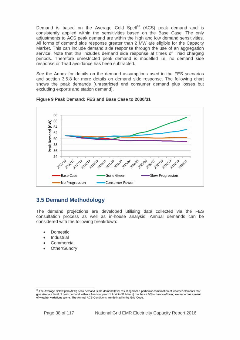
Page 38 of 117 National Grid EMR Electricity Capacity Report 2016
Demand is based on the Average Cold Spell18 (ACS) peak demand and isconsistently applied within the sensitivities based on the Base Case. The onlyadjustments to ACS peak demand are within the high and low demand sensitivities.All forms of demand side response greater than 2 MW are eligible for the CapacityMarket. This can include demand side response through the use of an aggregationservice. Note that this includes demand side response at times of Triad chargingperiods. Therefore unrestricted peak demand is modelled i.e. no demand sideresponse or Triad avoidance has been subtracted.
See the Annex for details on the demand assumptions used in the FES scenariosand section 3.5.8 for more details on demand side response. The following chartshows the peak demands (unrestricted end consumer demand plus losses butexcluding exports and station demand).
Figure 9 Peak Demand: FES and Base Case to 2030/31
3.5 Demand Methodology
The demand projections are developed utilising data collected via the FESconsultation process as well as in-house analysis. Annual demands can beconsidered with the following breakdown:
Domestic Industrial Commercial Other/Sundry
18 The Average Cold Spell (ACS) peak demand is the demand level resulting from a particular combination of weather elements thatgive rise to a level of peak demand within a financial year (1 April to 31 March) that has a 50% chance of being exceeded as a resultof weather variations alone. The Annual ACS Conditions are defined in the Grid Code.
54
56
58
60
62
64
66
68
Pe
akD
em
and
(GW
)
Base Case Gone Green Slow Progression
No Progression Consumer Power
Page 39 of 117 National Grid EMR Electricity Capacity Report 2016
3.5.1 Domestic
National Grid creates domestic demand by using a bottom up method. This looks atthe breakdown of the components of domestic demand. These components are listedbelow and each is projected individually which, when aggregated, form domesticdemand for each scenario.
Appliances – a regression trend method flexed by the application of primaryassumptions and appliance number caps.
Resistive heat – a new methodology has been applied with the use ofmodelling by Delta-ee. This produces a relatively gentle increase in demandconsistent with the growth in the number of new houses.
Resistive hot water – The current hot water electrical heat demand comesfrom published statistics. Due to the projected reduction in heat pumps weexpect the power demand for hot water to rise in line with the increase in thehousing stock.
Lighting – regression analysis to determine numbers and consumption bybulb type. This is flexed between scenarios by applying different future takeup rates based on the assumptions and possible further policy intervention.
Domestic annual demand reduction (smart effect) – deterministic modellingusing a smart meter roll out profile, project outcome data, such as theCustomer-Led Network Revolution19, and perceived customer engagementrates. This percentage is applied to the underlying domestic demand.
Heat pumps – using data from a bespoke Delta-ee model the assumption isnow that heat pumps, because of their associated infrastructural changes todomestic heating systems, will not be as prevalent as previously thought,except in the Gone Green scenario. Energy efficiency improvements areassumed annually based on manufacturer engagement feedback.
Electric Vehicles – a deterministic approach profiling purchase rates ofdifferent types of electric vehicles based on stakeholder feedback. This iscombined with statistics on journey length in order to assess the associatedelectrical demand.
3.5.2 Industrial
Industrial demand scenarios are created using a new model developed by Arup, inconjunction with Oxford Economics and National Grid. It is a modular model withthree basic components; the first being a macro-economic module which is aforecasting tool that generates long run forecasts for economic activity by sector, thesecond is an energy demand module which is a modelling tool which projects thesector energy demand based on measures of economic activity, prices andtemperature and the third is an energy technology module which is a bottom uptechnology investment simulation tool. This model is run four times, once for eachscenario, with the relevant scenario assumptions entered as inputs to give therequired outputs.
3.5.3 Commercial
The same new approach as in the industrial sector has been adopted this year,where the model is utilised to simulate the commercial sector.
19http://www.networkrevolution.co.uk/
Page 40 of 117 National Grid EMR Electricity Capacity Report 2016
3.5.4 Other/Sundry
These are the demand components which do not fall directly into the categoriesabove. For example, losses which are a function of the total demand figure,interconnector flows or micro-generation which is required in order to translate theFES total energy demand into a distribution or transmission demand definition.
3.5.5 Peak Demands
Once the assessment of underlying annual demand is created a recent historicalrelationship of annual to peak demand is applied. This creates an underlying peakdemand to which peak demand components that history cannot predict is added. Forexample, demand side response, electric vehicle charging or heat pump demand attimes of peak demand on the transmission system.The overlays to peak demand are;
Electric vehicles – based on the projected numbers, the potential user groupsare assessed, how and when they could be charging (constrained andunconstrained), and data from recently published trials are incorporated.
Heat pumps – using the number of heat pumps and heat demand, data frommanufacturers and trial within day profiles combined with performancestatistics and historical weather trends are used in order to determine theelectrical heat demand at peak.
Micro-generation – using the projection capacities by type and a peak loadfactor assumption, an assessment on the micro-generation levels at peak.
Losses – as with annual demand, this is a function of total peak demand. Industrial & Commercial Demand Side Response – created using desktop
research and assumptions of future efficiency improvements. Domestic peak response – as with annual demand this starts with the smart
meter roll out numbers, project outcome data and perceived customerengagement rates. From this results a percentage peak demand reduction.This percentage factor is then applied to the peak demand.
3.5.6 Calibration
Both annual and peak demands are calibrated. Annual demands are calibrated to theprevious year’s historical annual demand figures as published by DECC. Peakdemand is calibrated with weather corrected metered transmission demand.
3.5.7 Results
The results of the described methods provided are shown below in Annex. For amore detailed description of the FES scenarios please refer the FES document20;however, note that the demand is defined differently in the FES document to thatshown below which is unrestricted end consumer demand plus losses excludingexports and station demand.
20http://fes.nationalgrid.com/fes-document/

Page 41 of 117 National Grid EMR Electricity Capacity Report 2016
3.5.8 Demand Side Response
In the FES, DSR has been defined as a deliberate change to an end user’s naturalpattern of metered electricity consumption brought about by a signal from anotherparty. That is, demand shifting or demand reduction and not the use of generators tosubstitute the supply source. So, for instance, Triad avoidance is made up of bothdemand reduction (we estimate about 63%) and switching to an alternative supplysource. Within our definition of DSR we consider only the demand reductionelement.
The magnitude of the DSR will be dependent on what the market place offers andwhere the most value can be realised. As yet there is uncertainty as to what formthese value streams will take.
Modification to the Balancing and Settlement Code will require certain businesses tobe settled half hourly which should introduce a driver for businesses to use lesspower at peak, as power prices should be at their highest.
From winter 2017/18 those DSR providers which have an agreement under thecapacity market will be available and, it is assumed, they will remain in placethereafter. In the same year, we believe that DSR under Short Term OperatingReserve (STOR) will be available to the Capacity Market, where they will be able toaccess additional revenues. Thereafter new markets and revenue streams will openup, as a result of this changing environment, with profiles trending downwardstowards their maximum reduction values, which they all achieve by 2030. The rate ofchange depends upon the scenario’s conditions.
For the Gone Green scenario, a higher technical uptake rate and a higher utilisationrate of DSR is assumed. This is because the price of electricity will be high, there willbe greater peak demand and hence there will be relatively larger savings to be made.There will also be a greener ambition to encourage such behaviour changes.Batteries, in the latter half of the period, will pull down the requirement for true DSRas we view batteries as a form of generation when they are discharging. In NoProgression the cost of power will be lower and so the savings will be much less;consequently, a lower figure is assumed. For Slow Progression and ConsumerPower mid-ranges are assumed. However, Consumer Power sees significantincreases in battery storage and on-site generation. By the end of the period there isonly a residual amount of DSR available.
The projections of the industrial and commercial DSR profile reductions havechanged since the last FES publication. Figure 10 illustrates this year’s view.
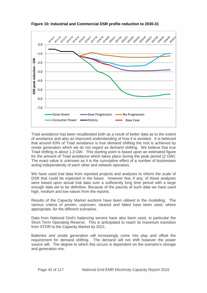
Page 42 of 117 National Grid EMR Electricity Capacity Report 2016
Figure 10: Industrial and Commercial DSR profile reduction to 2030-31
Triad avoidance has been recalibrated both as a result of better data as to the extentof avoidance and also an improved understanding of how it is avoided. It is believedthat around 63% of Triad avoidance is true demand shifting the rest is achieved byonsite generation which we do not regard as demand shifting. We believe that trueTriad shifting is about 1.3 GW. This starting point is based upon an estimated figurefor the amount of Triad avoidance which takes place during the peak period (2 GW).The exact value is unknown as it is the cumulative effect of a number of businessesacting independently of each other and network operators.
We have used trial data from reported projects and analyses to inform the scale ofDSR that could be expected in the future. However few, if any, of these analyseswere based upon actual trial data over a sufficiently long time period with a largeenough data set to be definitive. Because of the paucity of such data we have usedhigh, medium and low values from the reports.
Results of the Capacity Market auctions have been utilised in the modelling. Thevarious criteria of proven, unproven, cleared and failed have been used, whereappropriate, for the different scenarios.
Data from National Grid’s balancing service have also been used, in particular theShort Term Operating Reserve. This is anticipated to reach its maximum transitionfrom STOR to the Capacity Market by 2021.
Batteries and onsite generation will increasingly come into play and offset therequirement for demand shifting. The demand will not shift however the powersource will. The degree to which this occurs is dependent on the scenario’s storageand generation mix.
-7.0
-6.0
-5.0
-4.0
-3.0
-2.0
-1.0
0.0
DSR
pe
akre
du
ctio
n-
GW
Gone Green Slow Progression No Progression
Consumer Power History CentralBase Case
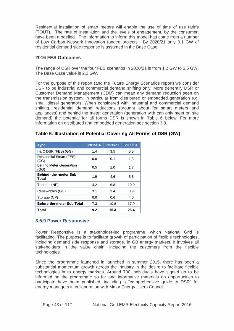
Page 43 of 117 National Grid EMR Electricity Capacity Report 2016
Residential installation of smart meters will enable the use of time of use tariffs(TOUT). The rate of installation and the levels of engagement, by the consumer,have been modelled. The information to inform this model has come from a numberof Low Carbon Network Innovation funded projects. By 2020/21 only 0.1 GW ofresidential demand side response is assumed in the Base Case.
2016 FES Outcomes
The range of DSR over the four FES scenarios in 2020/21 is from 1.2 GW to 3.5 GW.The Base Case value is 2.2 GW.
For the purpose of this report (and the Future Energy Scenarios report) we considerDSR to be industrial and commercial demand shifting only. More generally DSR orCustomer Demand Management (CDM) can mean any demand reduction seen onthe transmission system, in particular from distributed or embedded generation e.g.small diesel generators. When considered with industrial and commercial demandshifting, residential demand reductions (brought about for smart meters andappliances) and behind the meter generation (generation with can only meet on sitedemand) the potential for all forms DSR is shown in Table 6 below. For moreinformation on distributed and embedded generation see section 3.8.
Table 6: Illustration of Potential Covering All Forms of DSR (GW)
Type 2015/16 2020/21 2030/31
I & C DSR (FES) (GG) 1.4 3.5 5.5
Residential Smart (FES)(GG)
0.0 0.1 1.3
Behind Meter Generation(GG)
0.5 1.0 1.7
Behind -the -meter SubTotal
1.9 4.6 8.5
Thermal (NP) 4.2 6.8 10.0
Renewables (GG) 3.1 3.4 3.9
Storage (CP) 0.0 0.6 4.0
Before-the-meter Sub Total 7.3 10.8 17.9
Total 9.2 15.4 26.4
3.5.9 Power Responsive
Power Responsive is a stakeholder-led programme, which National Grid isfacilitating. The purpose is to facilitate growth of participation of flexible technologies,including demand side response and storage, in GB energy markets. It involves allstakeholders in the value chain, including the customers from the flexibletechnologies.
Since the programme launched in launched in summer 2015, there has been asubstantial momentum growth across the industry in the desire to facilitate flexibletechnologies in to energy markets. Around 700 individuals have signed up to beinformed on the programme so far and informative materials on opportunities toparticipate have been published, including a “comprehensive guide to DSR” forenergy managers in collaboration with Major Energy Users Council.

Page 44 of 117 National Grid EMR Electricity Capacity Report 2016
The impact we would expect as a result of activity is more interest in, and ultimatelygreater participation of flexible technologies in energy markets. Some evidence ofthis happening so far has been the increase in Triad Avoidance participation over thepast winter (up to 2GW from around 1GW) and procurement by National Grid of310MW Demand Turn Up, a new trial service run for the first time this year.
3.6 Generation Capacity until 2020/21
The generation forecast until 2020/21 has been created for the five year period2016/17 to 2020/21. It supports the DFA Incentive which is instrumental inrecommending a capacity to secure. This forecast is based on the latest marketintelligence and an economic assessment and provides a view of what thegeneration mix may look like over the five year period. The outcome is that the BaseCase sits within the envelope established by the Future Energy Scenarios; seeFigure 11.
Figure 11: FES 2016 Transmission connected nameplate capacity to 2020/21
Table 7: Transmission connected nameplate capacity (GW) to 2020/21
Capacity GW 2015/16 2016/17 2017/18 2018/19 2019/20 2020/21
Gone Green 70.5 67.9 64.9 65.3 63.5 61.1
Slow Progression 70.5 68.1 65.9 65.9 64.5 64.3
No Progression 70.5 68.7 67.3 66.7 67.5 65.2
Consumer Power 70.5 67.6 66.3 65.0 61.8 60.9
Base Case 70.5 67.8 66.6 65.4 64.1 61.4
56
58
60
62
64
66
68
70
72
2015/16 2016/17 2017/18 2018/19 2019/20 2020/21
Inst
alle
dC
apac
ity
(GW
)
Gone Green Slow Progression No Progression
Consumer Power Base Case
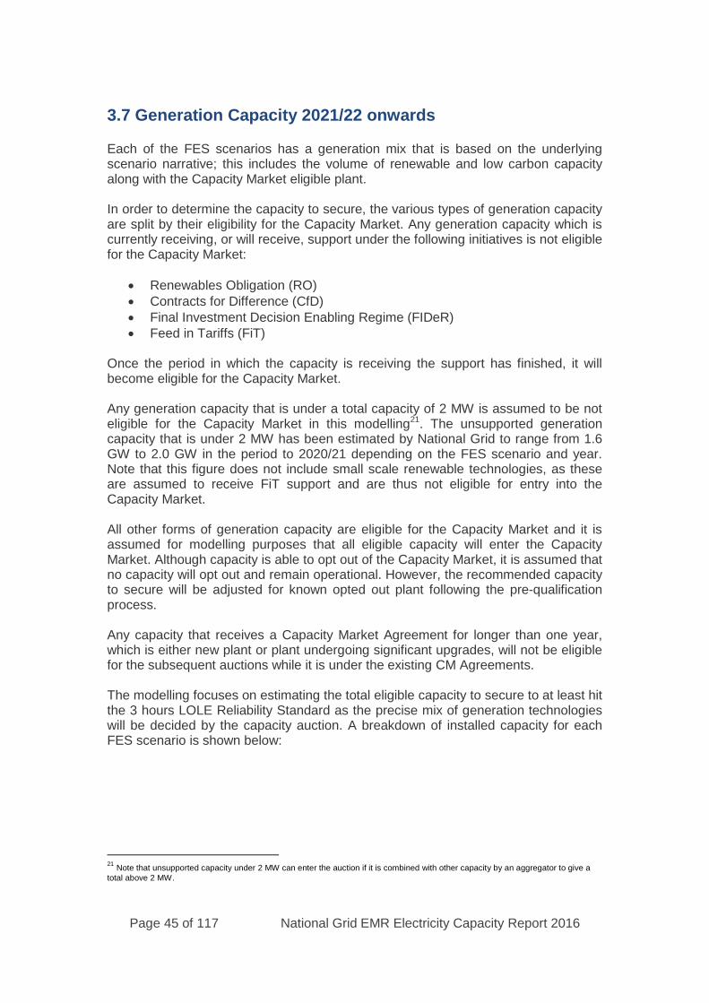
Page 45 of 117 National Grid EMR Electricity Capacity Report 2016
3.7 Generation Capacity 2021/22 onwards
Each of the FES scenarios has a generation mix that is based on the underlyingscenario narrative; this includes the volume of renewable and low carbon capacityalong with the Capacity Market eligible plant.
In order to determine the capacity to secure, the various types of generation capacityare split by their eligibility for the Capacity Market. Any generation capacity which iscurrently receiving, or will receive, support under the following initiatives is not eligiblefor the Capacity Market:
Renewables Obligation (RO) Contracts for Difference (CfD) Final Investment Decision Enabling Regime (FIDeR) Feed in Tariffs (FiT)
Once the period in which the capacity is receiving the support has finished, it willbecome eligible for the Capacity Market.
Any generation capacity that is under a total capacity of 2 MW is assumed to be noteligible for the Capacity Market in this modelling21. The unsupported generationcapacity that is under 2 MW has been estimated by National Grid to range from 1.6GW to 2.0 GW in the period to 2020/21 depending on the FES scenario and year.Note that this figure does not include small scale renewable technologies, as theseare assumed to receive FiT support and are thus not eligible for entry into theCapacity Market.
All other forms of generation capacity are eligible for the Capacity Market and it isassumed for modelling purposes that all eligible capacity will enter the CapacityMarket. Although capacity is able to opt out of the Capacity Market, it is assumed thatno capacity will opt out and remain operational. However, the recommended capacityto secure will be adjusted for known opted out plant following the pre-qualificationprocess.
Any capacity that receives a Capacity Market Agreement for longer than one year,which is either new plant or plant undergoing significant upgrades, will not be eligiblefor the subsequent auctions while it is under the existing CM Agreements.
The modelling focuses on estimating the total eligible capacity to secure to at least hitthe 3 hours LOLE Reliability Standard as the precise mix of generation technologieswill be decided by the capacity auction. A breakdown of installed capacity for eachFES scenario is shown below:
21Note that unsupported capacity under 2 MW can enter the auction if it is combined with other capacity by an aggregator to give a
total above 2 MW.
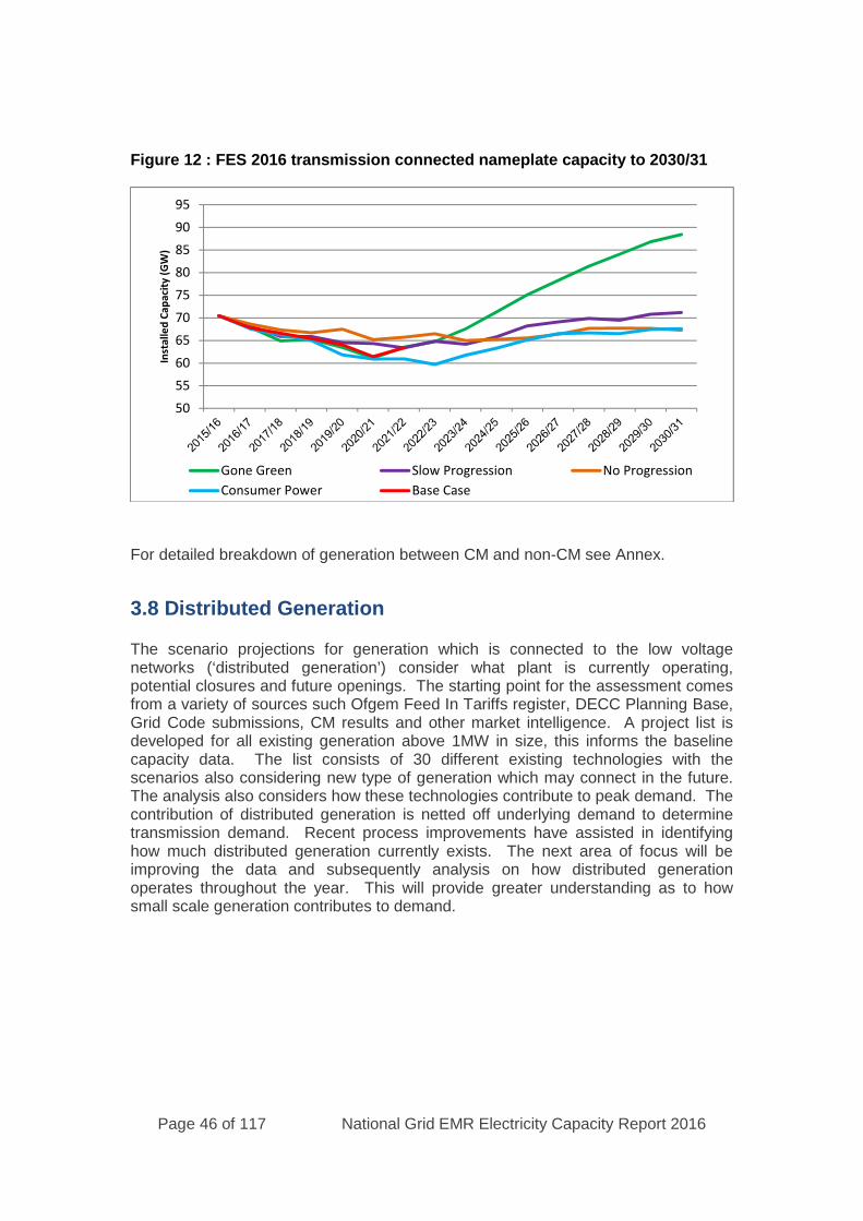
Page 46 of 117 National Grid EMR Electricity Capacity Report 2016
Figure 12 : FES 2016 transmission connected nameplate capacity to 2030/31
For detailed breakdown of generation between CM and non-CM see Annex.
3.8 Distributed Generation
The scenario projections for generation which is connected to the low voltagenetworks (‘distributed generation’) consider what plant is currently operating,potential closures and future openings. The starting point for the assessment comesfrom a variety of sources such Ofgem Feed In Tariffs register, DECC Planning Base,Grid Code submissions, CM results and other market intelligence. A project list isdeveloped for all existing generation above 1MW in size, this informs the baselinecapacity data. The list consists of 30 different existing technologies with thescenarios also considering new type of generation which may connect in the future.The analysis also considers how these technologies contribute to peak demand. Thecontribution of distributed generation is netted off underlying demand to determinetransmission demand. Recent process improvements have assisted in identifyinghow much distributed generation currently exists. The next area of focus will beimproving the data and subsequently analysis on how distributed generationoperates throughout the year. This will provide greater understanding as to howsmall scale generation contributes to demand.
50
55
60
65
70
75
80
85
90
95
Inst
alle
dC
apac
ity
(GW
)
Gone Green Slow Progression No Progression
Consumer Power Base Case

Page 47 of 117 National Grid EMR Electricity Capacity Report 2016
Figure 13: Distributed generation nameplate capacity (excluding Solar) to2020/21 (GW)
Table 8: Distributed generation nameplate capacity (GW)
Capacity GW 2015/16 2016/17 2017/18 2018/19 2019/20 2020/21
Gone Green 12.0 12.5 13.1 14.0 15.2 15.8
Slow Progression 12.0 12.5 13.3 14.3 15.1 15.3
No Progression 12.0 12.6 13.5 14.6 15.3 15.5
Consumer Power 12.0 12.6 13.6 15.2 16.2 16.8
Base Case 12.0 12.6 13.6 14.9 15.7 16.0
Figure 14: Distributed Generation (excluding Solar) to 2030/31 (GW)
10
11
12
13
14
15
16
17
18
2015/16 2016/17 2017/18 2018/19 2019/20 2020/21
Insta
lled
Cap
acit
y(G
W)
Gone Green Slow Progression No ProgressionConsumer Power Base Case
10
12
14
16
18
20
22
24
26
28
30
Gone Green Slow Progression No Progression
Consumer Power Base Case
Page 48 of 117 National Grid EMR Electricity Capacity Report 2016
3.9 Generation Methodology
The power supply transmission backgrounds use a rule based deterministicapproach. An individual assessment of each power station (at a unit level whereappropriate) is completed, taking into account a wide spectrum of information,analysis and intelligence from various sources.
The scenario narratives provide the uncertainty envelope that determines theemphasis placed on the different types of generation technology within eachscenario. Each power station will then be placed accordingly within their technologystack.
The placement of a power station will be determined by a number of factors, such asmarket intelligence, energy policy and legislation. Project status and economics,which are applicable to that particular power station, were also taken into account.The contracted background or Transmission Entry Capacity (TEC) Register22
provides the starting point for the analysis of power stations which require access tothe National Electricity Transmission System (NETS). It provides a list of powerstations which are using, or planning to make use, of the NETS. Although thecontracted background provides the basis for the majority of the entries into thegeneration backgrounds, the analysis is not limited to generators with a signedconnection agreement. Other projects where information has been received about inthe very early phases of scoping pre connection agreement are also taken intoaccount.
For power generation connecting to the distributed system alternative sources of datawill be used as the starting point for assessment, such as the Ofgem Feed In Tariffsregister or DECC Planning Base, as the starting point for the assessment.
The generation backgrounds are then built up to meet the Reliability Standard from2020/21 onwards.
3.9.1 Contracted Background
This contracted background provides a list of power stations which have anagreement to gain access rights to NETS; now and in the future. It provides valuableup to date information regarding any increase and decreases to a power stationTransmission Entry Capacity which provides an indication of how a particular plantmay operate in future years. This is then overlaid with market intelligence for thatparticular plant and/or generation technology type.
3.9.2 Market Intelligence
This section covers how market intelligence gathered through stakeholderengagement along with more general information is used to help determine whichgeneration is likely to connect during the FES study period.
22http://www2.nationalgrid.com/UK/Services/Electricity-connections/Industry-products/TEC-Register/

Page 49 of 117 National Grid EMR Electricity Capacity Report 2016
Developer Profile
This information relates to the developer of a certain project or portfolio of projectsand provides an insight into how and when these projects may develop. Examples ofinformation taken into account under this area are;
Is the developer a portfolio player who may have a number of potentialprojects at different stages of the process in which case intelligence isgathered on the developers “preferred” or “priority” projects, or is it amerchant developer who is looking to become active within the electricitymarket?
How active is the developer in the GB electricity market
Technology
This area looks specifically at future and developing technologies to gauge howmuch of a part certain emerging generation types may play in the generationbackgrounds. Examples of information taken into account in this area are:
At what stage of development or deployment is the technology, e.g. has thetechnology been proven as a viable source of electricity generation?
Have there been trial/pilot projects carried out as with technologies such aswave and tidal?
Has there been a commercial scale roll out of the technology followingsuccessful trial/pilot schemes?
Is there Government backing and support for the new technology? Are there any industry papers or research regarding the roll out of new
technologies in terms of the potential scale of deployment should thetechnology be proven?
Financial Markets
Information relating to the financial markets is also a consideration in terms of howeasy it will be for the developer to raise the capital to fully develop the project e.g. offthe balance sheet or via the capital markets.
Consideration is also given to the economics for different types of generation, interms of spark, dark and clean spreads, electricity wholesale prices and the impact ofthe carbon price which may impact the operational regime on a technology and/orplant specific basis
3.9.3 FES Plant Economics
This area is a key feed in to the power generation backgrounds and exploreseconomic viability and how a particular plant or group of plants could operate in themarket now and in the future. The Short Run Marginal Cost (SRMC) of the existingpower station fleet has been a focus of the 2016 analysis. The model calculates theSRMC for transmission connected power stations which will be used to inform thepower generation backgrounds:
Computed the SRMCs for each quarter at unit level Dispatched according to their SRMCs (low-carbon and CHP set as must-run) Profit and loss for each power station is calculated based on its running hours
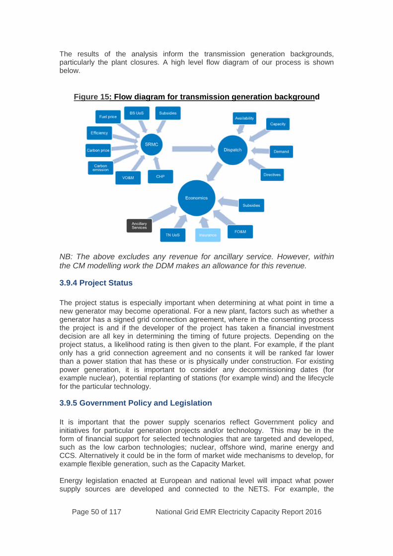
Page 50 of 117 National Grid EMR Electricity Capacity Report 2016
The results of the analysis inform the transmission generation backgrounds,particularly the plant closures. A high level flow diagram of our process is shownbelow.
Figure 15: Flow diagram for transmission generation background
NB: The above excludes any revenue for ancillary service. However, withinthe CM modelling work the DDM makes an allowance for this revenue.
3.9.4 Project Status
The project status is especially important when determining at what point in time anew generator may become operational. For a new plant, factors such as whether agenerator has a signed grid connection agreement, where in the consenting processthe project is and if the developer of the project has taken a financial investmentdecision are all key in determining the timing of future projects. Depending on theproject status, a likelihood rating is then given to the plant. For example, if the plantonly has a grid connection agreement and no consents it will be ranked far lowerthan a power station that has these or is physically under construction. For existingpower generation, it is important to consider any decommissioning dates (forexample nuclear), potential replanting of stations (for example wind) and the lifecyclefor the particular technology.
3.9.5 Government Policy and Legislation
It is important that the power supply scenarios reflect Government policy andinitiatives for particular generation projects and/or technology. This may be in theform of financial support for selected technologies that are targeted and developed,such as the low carbon technologies; nuclear, offshore wind, marine energy andCCS. Alternatively it could be in the form of market wide mechanisms to develop, forexample flexible generation, such as the Capacity Market.
Energy legislation enacted at European and national level will impact what powersupply sources are developed and connected to the NETS. For example, the
Page 51 of 117 National Grid EMR Electricity Capacity Report 2016
renewable energy target for 2020 is intended to reduce reliance on high carbon fossilfuels by promoting renewable sources, making it very likely that the NETS willexperience much more intermittent renewable capacity. Another example is the plantthat may have to be modified to comply with environmental directives, such as theLarge Combustion Plant Directive, Industrial Emissions Directive and potentiallyMedium Combustion Plant Directive. This legislation places restrictions on thenumber of running hours for fossil fuel power generation plants with regard to theharmful waste gases that they emit, unless investments are made to reduce thisimpact, and will affect decisions on whether to invest in new plants or maintainexisting facilities.
3.9.6 Reliability Standard
The power generation backgrounds were developed for each of the scenarios basedon the information gathered, as explained above. The 2016 power generationsbackgrounds are developed to both meet demand and to meet the ReliabilityStandard of 3 hours LOLE. In the years up to 2017/18, the generation backgroundsare driven by more granular intelligence and therefore LOLE can vary quitesignificantly year to year within this period. If 2016/17 LOLE is predicted to rise above3 hours then National Grid and Ofgem have agreed to meet the Reliability Standardfrom procurement of Contingency Balancing Reserve (CBR). From 2017/18 onwards,the backgrounds are developed to not exceed 3 hours LOLE under the CapacityMarket (CM).
3.10 Interconnector Capacity Assumptions
We derived our interconnector capacity assumptions from an analysis of individualprojects. We have anonymised the data by showing only the total capacity per year,due to commercial sensitivities.
We identified potential projects and their expected commissioning dates to connect toGB. This information was from a range of sources including the electricity EuropeanNetwork of Transmission System Operators (ENTSO-e) ten-year networkdevelopment plan, 4C Offshore and the European Commission. Where only acommissioning year was given we assumed the date to be 1 October of that year.We assessed each project individually against political, economic, social,technological and environmental factors to determine which interconnector projectswould be built under each scenario. If it did not meet the minimum criteria weassumed it will not be delivered in the given scenario, or that it will be subject to acommissioning delay. We calculated this delay using a generic accelerated high-voltage direct current (HVDC) project timeline. All projects which have reached finalsanction are delivered, though they may be subject to delays in some scenarios.
In all scenarios we assumed that the supply chain has enough capacity to deliver allinterconnector projects. We have assumed that the cap and floor regime is requiredfor all scenarios other than Consumer Power which is market driven. Additionally, weassumed that only one project between GB and another market can be delivered atany one time under No Progression. For the Base Case we have selected GoneGreen for the years to 2020/21 and Slow Progression for the later years.
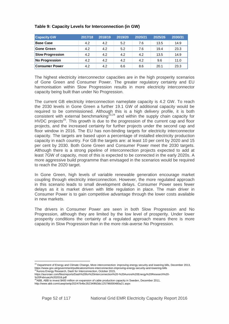
Page 52 of 117 National Grid EMR Electricity Capacity Report 2016
Table 9: Capacity Levels for Interconnection (in GW)
The highest electricity interconnector capacities are in the high prosperity scenariosof Gone Green and Consumer Power. The greater regulatory certainty and EUharmonisation within Slow Progression results in more electricity interconnectorcapacity being built than under No Progression.
The current GB electricity interconnection nameplate capacity is 4.2 GW. To reachthe 2030 levels in Gone Green a further 19.1 GW of additional capacity would berequired to be commissioned. Although this is a high delivery profile, it is bothconsistent with external benchmarking23,24 and within the supply chain capacity forHVDC projects25. This growth is due to the progression of the current cap and floorprojects, and the increased certainty for further projects under the second cap andfloor window in 2016. The EU has non-binding targets for electricity interconnectorcapacity. The targets are based upon a percentage of installed electricity productioncapacity in each country. For GB the targets are: at least 10 per cent by 2020 and 15per cent by 2030. Both Gone Green and Consumer Power meet the 2030 targets.Although there is a strong pipeline of interconnection projects expected to add atleast 7GW of capacity, most of this is expected to be connected in the early 2020s. Amore aggressive build programme than envisaged in the scenarios would be requiredto reach the 2020 target.
In Gone Green, high levels of variable renewable generation encourage marketcoupling through electricity interconnection. However, the more regulated approachin this scenario leads to small development delays. Consumer Power sees fewerdelays as it is market driven with little regulation in place. The main driver inConsumer Power is to gain competitive advantage through the lower costs availablein new markets.
The drivers in Consumer Power are seen in both Slow Progression and NoProgression, although they are limited by the low level of prosperity. Under lowerprosperity conditions the certainty of a regulated approach means there is morecapacity in Slow Progression than in the more risk-averse No Progression.
23Department of Energy and Climate Change, More interconnection: improving energy security and lowering bills, December 2013,
https://www.gov.uk/government/publications/more-interconnection-improving-energy-security-and-lowering-bills24
Aurora Energy Research, Dash for Interconnection, October 2015,https://auroraer.com/files/reports/Dash%20for%20interconnection%20-%20Aurora%20Energy%20Research%20-%20February%202016.pdf25
ABB, ABB to invest $400 million on expansion of cable production capacity in Sweden, December 2011,http://www.abb.com/cawp/seitp202/47b4bc352349fd3dc125796000480a21.aspx
Capacity GW 2017/18 2018/19 2019/20 2020/21 2025/26 2030/31
Base Case 4.2 4.2 5.2 7.6 13.5 14.9
Gone Green 4.2 4.2 5.2 7.6 19.4 23.3
Slow Progression 4.2 4.2 4.2 4.2 13.5 14.9
No Progression 4.2 4.2 4.2 4.2 9.6 11.0
Consumer Power 4.2 4.2 6.6 8.6 20.1 23.3

Page 53 of 117 National Grid EMR Electricity Capacity Report 2016
Figure 16: Annual interconnector net flows
As with all interconnector flows, annual flows, shown in
Figure 16, are driven by prices. Until the mid-2020s the carbon floor priceencourages cheaper continental generation to be imported into GB across all of thescenarios. Later in the period the increasing proportions of renewable generation andthe price coupling effects of electricity interconnection bring the market prices closertogether. While this reduces the net annual flows, GB retains a net import position.
Figure 17: Peak interconnector net flows
In FES 2016 we define peak flows, shown in Figure 17, as the flows which could berelied on to supply winter peak demand when Great Britain needs imports. This is a
Page 54 of 117 National Grid EMR Electricity Capacity Report 2016
more extreme measure than average flows at ACS (average cold spell) conditions.Actual flows at times of ACS peak demand could differ significantly from thesefigures due to the impact of other factors such as wind generation and the stresslevel of connected markets.
We commissioned external consultants (Baringa) to assess the flows between GBand connected countries for each scenario using a pan-European market model.Flows were modelled for each scenario based on FES 2015 demand and generationdata, FES 2016 electricity interconnector capacity, and the consultancy’s owndataset for non-GB countries.
However, it should be noted that these peak figures aren’t used in the CM modellingas that uses probabilistic distributions from Baringa’s pan-European market model(except for 2018/19 which uses, as a base assumption, the de-rating factors used inthe 2019/20 T-4 auction, set by DECC, applied to the interconnectors – see 3.11.5).
3.11 Sensitivity Descriptions and Justifications
The analysis assumes that the Future Energy Scenarios (FES) will cover uncertaintyby incorporating ranges for annual and peak demand, Demand Side Response(DSR), interconnection and generation. In addition to the FES scenarios, a DECCScenario has been included for information but hasn’t been included in the LWRcalculation to ensure the recommendation is fully independent by basing it on andaround National Grid’s Base Case and four FES scenarios.
While the FES scenarios vary many variables (see list of primary assumptions inAnnex 8.2) the sensitivities vary only one variable at a time. Each of the sensitivitiesis considered credible as it is evidence based i.e. it has occurred in recent history oris to address statistical uncertainty caused by the small sample sizes used for someof the input variables. The sensitivities cover uncertainty in station peak availabilities,weather, wind, peak demand forecast performance and non-delivery of contractedcoal capacity. In addition, for 2018/19 only, there are sensitivities covering a range ofinterconnector peak flows.
To provide the reference case to which the sensitivities have been applied, a BaseCase has been introduced. Up to 2020/21, the Base Case consists of our centralview of the demand and generation backgrounds which aligns with the DFA Incentiveand aims to reduce the likelihood of over or under securing capacity therebyminimising the associated costs to consumer. From 2021/22 the Base Case takesthe demand and generation mix from the Slow Progression scenario.
The sensitivities are described below. However, there are small differences in theway that these sensitivities were applied to each of the individual year runs: theelements that are different in each year are described in the chapters relating tothose years.
3.11.1 Low Wind (at times of cold weather)
As detailed in Section 2.6.2, recent statistical analysis undertaken by DurhamUniversity and Heriot-Watt University recommended the inclusion of a low windsensitivity. In line with the recommendation, this sensitivity models the impact oflower wind generation than the base assumption at times of cold weather (i.e. attimes of high demand). To model this sensitivity a scaling of 0.8 is used (i.e. wind
Page 55 of 117 National Grid EMR Electricity Capacity Report 2016
output is reduced linearly from 100% of its unscaled value to 80% for daily peakdemands between the thresholds of 92% and 102% of peak demand..
3.11.2 High Wind (at times of cold weather)
As detailed in Section 2.6.2, recent statistical analysis undertaken by DurhamUniversity and Heriot-Watt University recommended the inclusion of a high windsensitivity. In line with the recommendation, this sensitivity models the impact ofhigher wind generation than the base assumption at times of cold weather (i.e. attimes of high demand). To model this sensitivity a scaling of 1.0 is used i.e. thissensitivity assumes that wind output is independent of daily peak demand).
3.11.3 High Plant Availabilities
The high and low plant availability sensitivities address the statistical uncertaintyassociated with determining the mean availabilities of each fuel type. The meanavailabilities are determined based on the last 7 years, which is too small a samplesize (i.e. just 7 data points) to be confident that the means of these distributions willbe statistically representative of what could happen in the future. The plantavailability sensitivities are not intended to address concerns of whether the baseavailability assumptions are too high or too low, and nor are they intended to makepredictions as to what levels of plant availability we believe will occur. These arepurely statistical sensitivities to address the uncertainty in calculating mean valuesfrom a small number of points. To allow for this in the modelling it assumes for two ofthe largest contributing generation technologies (nuclear and CCGT) a higher meanavailability than the base assumption (see 2.3.2). This higher availability is alsoapplied to any capacity for these technologies contracted in previous auctions.
For existing nuclear the availability increases by over 4% from just 84% to ~89% andfor CCGTs by 2% from 90% to 92% in 2020/21 and from 88% to 90% in 2017/18 and2018/19. These higher availabilities are based on one standard deviation above themean of observed figures from the last seven years. Coal availabilities haven’t beenflexed as coal availabilities show very little variance over the last seven years. Inaddition, other technologies haven’t been flexed to allow for diversity as it would beunlikely all technologies would be simultaneously at their high availability levels.
In 2017/18 for example, adjusting availabilities has an impact on the diversity of plantand therefore a small impact on the de-rated total required. However, it clearly has alarge impact on the name plate capacity total. These adjustments have been appliedto the technologies that are both large in aggregate GWs and have shown varianceacross the sample. In addition to these sensitivities being the statistically correctthing to do, they also have the added advantage of providing greater granularity tothe LWR calculation.
3.11.4 Low Plant Availabilities
The low plant availability sensitivity assumes for two of the largest contributinggeneration technologies (nuclear and CCGT) a lower mean availability than the baseassumption (see 2.3.2). For nuclear the availability reduces from 84% to 80% and forCCGTs from 90% to 88% in 2020/21 and from 88% to 86% in 2017/18 and 2018/19.These lower availabilities are based on one standard deviation below the mean ofobserved figures from the last seven years.
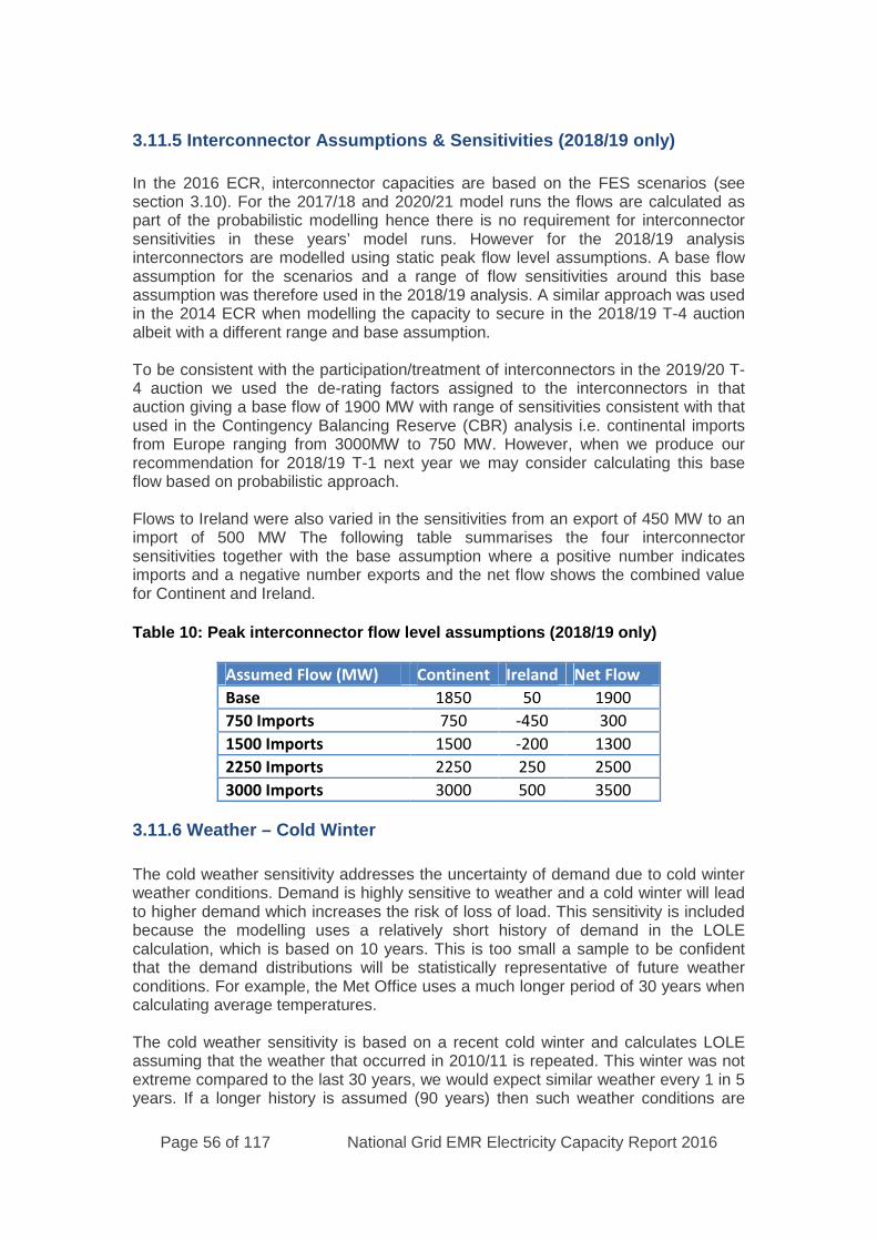
Page 56 of 117 National Grid EMR Electricity Capacity Report 2016
3.11.5 Interconnector Assumptions & Sensitivities (2018/19 only)
In the 2016 ECR, interconnector capacities are based on the FES scenarios (seesection 3.10). For the 2017/18 and 2020/21 model runs the flows are calculated aspart of the probabilistic modelling hence there is no requirement for interconnectorsensitivities in these years’ model runs. However for the 2018/19 analysisinterconnectors are modelled using static peak flow level assumptions. A base flowassumption for the scenarios and a range of flow sensitivities around this baseassumption was therefore used in the 2018/19 analysis. A similar approach was usedin the 2014 ECR when modelling the capacity to secure in the 2018/19 T-4 auctionalbeit with a different range and base assumption.
To be consistent with the participation/treatment of interconnectors in the 2019/20 T-4 auction we used the de-rating factors assigned to the interconnectors in thatauction giving a base flow of 1900 MW with range of sensitivities consistent with thatused in the Contingency Balancing Reserve (CBR) analysis i.e. continental importsfrom Europe ranging from 3000MW to 750 MW. However, when we produce ourrecommendation for 2018/19 T-1 next year we may consider calculating this baseflow based on probabilistic approach.
Flows to Ireland were also varied in the sensitivities from an export of 450 MW to animport of 500 MW The following table summarises the four interconnectorsensitivities together with the base assumption where a positive number indicatesimports and a negative number exports and the net flow shows the combined valuefor Continent and Ireland.
Table 10: Peak interconnector flow level assumptions (2018/19 only)
Assumed Flow (MW) Continent Ireland Net Flow
Base 1850 50 1900
750 Imports 750 -450 300
1500 Imports 1500 -200 1300
2250 Imports 2250 250 2500
3000 Imports 3000 500 3500
3.11.6 Weather – Cold Winter
The cold weather sensitivity addresses the uncertainty of demand due to cold winterweather conditions. Demand is highly sensitive to weather and a cold winter will leadto higher demand which increases the risk of loss of load. This sensitivity is includedbecause the modelling uses a relatively short history of demand in the LOLEcalculation, which is based on 10 years. This is too small a sample to be confidentthat the demand distributions will be statistically representative of future weatherconditions. For example, the Met Office uses a much longer period of 30 years whencalculating average temperatures.
The cold weather sensitivity is based on a recent cold winter and calculates LOLEassuming that the weather that occurred in 2010/11 is repeated. This winter was notextreme compared to the last 30 years, we would expect similar weather every 1 in 5years. If a longer history is assumed (90 years) then such weather conditions are
Page 57 of 117 National Grid EMR Electricity Capacity Report 2016
actually closer to the average but due to climate change a 30 year history may be amore suitable basis.
There are two further reasons why this sensitivity is included. Firstly, LOLE is ametric that is highly non-linear and excluding the sensitivity would fail to fully accountfor the non-linear impact of cold weather on LOLE and therefore understate itsimpact. This can be easily illustrated by considering two hypothetical scenarios bothof which meet the Reliability Standard but have significantly different impacts.
Over a ten year period this scenario has 3 hours LOLE in each year whichgives an average of 3 hours LOLE over the ten year period and thereforemeets the Reliability Standard and with mitigating actions could result in nocontrolled disconnections.
Over a ten year period this scenario has 30 hours LOLE in one year and 0hours LOLE in 9 other years which gives an average of 3 hours LOLE overthe ten year period and therefore meets the Reliability Standard but this timemitigating actions may not be able to prevent controlled disconnections –hence the impact on consumers is significantly different and demonstrateswhy LOLE as a first order measure fails to address this risk.
The final reason for including this sensitivity is reputational as this sensitivity is clearlycredible given that the winter was less than 6 years ago, wasn’t extreme and from apractical communications point it would be extremely difficult to defend a position thatdidn’t consider it in the calculation.
Section 2.5 contains further justification including academic research that supportsthe inclusion of the cold and warm winter sensitivities in the analysis.
3.11.7 Weather – Warm Winter
This warm weather sensitivity is included on the same statistical basis as coldweather, and ensures that the treatment of the uncertainty of demand due to weatheris unbiased. The warm weather sensitivity is based on a recent warm winter andcalculates LOLE assuming that the weather that occurred in 2006/07 is repeated.This winter was not extreme and when compared to the last 30 years, we wouldexpect similar weather every 1 in 15 years.
3.11.8 High Demand
In the 2015 ECR, the high and low demand sensitivities were based around therange of historical forecasting performance for Transmission level demand for thewinter ahead (see 2015 ECR for the rationale behind this). This produced anasymmetric range of demand sensitivities reflecting the tendency to overforecastdemand over recent years mainly due to the rapid growth in distributed generationand the lack of visibility of both capacity and generation data and secondly, theprolonged economic recession which suppressed demand longer than expected.These two factors may be less relevant in the future due to improved access to dataon distributed generation and the view by economists that a recession in GB of themagnitude seen recently is unlikely.
National Grid now has the DFA Incentive and an obligation to publish how it plans toimprove the demand forecasting process every year. Consequently, the demandsensitivities have been aligned with the ranges used within the incentives rather thanhistorical performance. The DFA Incentive for the T-1 auction has a symmetric range

Page 58 of 117 National Grid EMR Electricity Capacity Report 2016
of +/- 2% which forms the basis of the sensitivities in the 2016 ECR. We have notused the T-4 incentive range of +/- 4% as the incentive is weighted towards the T-1demand given that there is an opportunity (in the T-1 recommendation) to correctany forecast errors in the T-4 demand.
The high demand sensitivity covers the upper end of the range of uncertainty of theunderlying (i.e. weather-corrected) ACS peak demand forecast. This assumes peakdemand values that are 2% above the FES ACS peak demands.
3.11.9 Low Demand
The low demand sensitivity covers the lower end of the range of uncertainty of theunderlying (i.e. weather-corrected) ACS peak demand forecast. This assumes peakdemand values that are 2% below the FES ACS peak demands.
3.11.10 Non-delivery of Contracted Coal Capacity
Given the poor state of coal station economics, recent coal closure announcementsand the recent Government announcements around the future of coal, there is acredible risk that coal stations with CM contracts will close ahead of the delivery yearor coal stations opting out of the CM that had previous indicated they would beoperational will close. The Future Energy Scenarios already take account of “higherrisk non-delivery issues (”known knowns”) e.g. plants that have already announcedclosure or plants assumed to close under the conditions in the scenario frameworkfor particular scenarios.
In addition, the 2016 ECR includes a range of non-delivery sensitivities to cover thecredible risk of earlier than expected closures of coal stations assumed to begenerating in the FES. For example, stations with existing CM contracts (from the2018/19 or 2019/20 T-4 auctions) could close early; stations successful in futureauctions could close before the delivery year e.g. due to breakdowns beinguneconomic to repair; and there is a possibility that all coal stations could close withor without CM contracts.
If these adjustments for non-delivery are made prior to simulating the auctions in theDDM the model will assume a different new or existing plant is contracted instead,resulting in the same de-rated requirement as it is non-technology specific. Hencethese non-delivery sensitivities have been modelled by reducing the “outside CM”capacity after the DDM runs.
The non-delivery sensitivities deal with uncertain risks (“known unknowns”) for non-delivery and also assist with the granularity in the LWR calculation. A range of non-delivery sensitivities with incremental steps of 400 MW (around the de-rated capacityof a typical coal power station unit) have been modelled up to a maximum of 2800MW in 2017/18 (similar to the range modelled in the CBR analysis for 20167/17) and3600 MW in 2018/19 and 2020/21 (roughly equivalent to the de-rated capacity of two2 GW coal power stations).
3.11.11 Sensitivities Considered but Rejected
A number of alternative sensitivities were considered for inclusion but followingdiscussions with DECC and the PTE were rejected.

Page 59 of 117 National Grid EMR Electricity Capacity Report 2016
Dependence of Generating Units - The DDM implicitly assumes independencein availability of generating units. A number of commentators/consultancies havesuggested that this assumption is optimistic. For example, a fault in one unit canaffect the other units on site or a station transformer fault could affect more than oneunit or the operation of a station within a portfolio could be affected by the otherstations in that portfolio. However, the data available associated with these issues iseither very limited or difficult to interpret and translate for use into the future, makingit very difficult to quantify for modelling purposes. Hence this sensitivity was notincluded.
Renewable Plant Non-Delivery - This concept of this sensitivity was to reflectslippage in non-CM plants away from their connection and contract dates similar tothe CM non-delivery sensitivities. However, following discussions with DECC and thePTE it was agreed not to include this sensitivity since there is a credible range in thelevel of renewable generation connecting across the four FES scenarios and BaseCase.
Black Swan Events– These are defined as events that have low probability buthigh impact. Examples for GB would include large nuclear type faults, extremeweather e.g. Jan. 1986/7, significant technology closures due to economics or policyplus issues not yet identified (“unknown unknowns”). We have investigated nucleartype faults before and concluded that they were low probability and historically hadbeen rectified ahead of the following winter (albeit with stations operating at areduced capacity but this would be covered in the scenarios). We have alsoconsidered extreme cold weather (e.g. Jan.1986/87) combined with low wind, but thiswould involve changing more than one element which violates the principles behindthe sensitivities of only including credible outcomes and only changing one variable.Given this and given that economic or policy events relating to uncertainty aroundcoal will be addressed through the non-delivery sensitivities, we agreed with DECCand the PTE not to include any “black swan” event sensitivities.
3.12 15 years horizon
This section considers the overall level of de-rated capacity requirement in futureyears, not just the years of interest for this report (2017/18, 2018/29 and 2020/21). Itfocuses on the total requirement for CM-eligible capacity and does not split eachyear’s requirement into capacity secured in earlier years, T-1/transitional and T-4auctions. The requirement for 2017/18 was derived from the 2017/18 model runs(see chapter 6), the requirement in 2018/19 and 2019/20 from the 2018/19 modelruns (see Chapter 7) and the capacity requirement from 2020/21 to 2030/31 from themodel runs for 2020/21 (See Chapter 5). This section is included before the mainresults chapters to illustrate the ongoing requirement for CM-eligible capacity.
Figure 18 shows the range in modelled capacity requirement in future years includingany new / refurbished capacity secured in previous years.
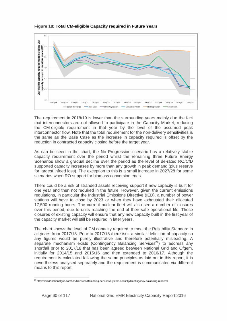
Page 60 of 117 National Grid EMR Electricity Capacity Report 2016
Figure 18: Total CM-eligible Capacity required in Future Years
The requirement in 2018/19 is lower than the surrounding years mainly due the factthat interconnectors are not allowed to participate in the Capacity Market, reducingthe CM-eligible requirement in that year by the level of the assumed peakinterconnector flow. Note that the total requirement for the non-delivery sensitivities isthe same as the Base Case as the increase in capacity required is offset by thereduction in contracted capacity closing before the target year.
As can be seen in the chart, the No Progression scenario has a relatively stablecapacity requirement over the period whilst the remaining three Future EnergyScenarios show a gradual decline over the period as the level of de-rated RO/CfDsupported capacity increases by more than any growth in peak demand (plus reservefor largest infeed loss). The exception to this is a small increase in 2027/28 for somescenarios when RO support for biomass conversion ends.
There could be a risk of stranded assets receiving support if new capacity is built forone year and then not required in the future. However, given the current emissionsregulations, in particular the Industrial Emissions Directive (IED), a number of powerstations will have to close by 2023 or when they have exhausted their allocated17,500 running hours. The current nuclear fleet will also see a number of closuresover this period, due to units reaching the end of their safe operational life. Theseclosures of existing capacity will ensure that any new capacity built in the first year ofthe capacity market will still be required in later years.
The chart shows the level of CM capacity required to meet the Reliability Standard inall years from 2017/18. Prior to 2017/18 there isn’t a similar definition of capacity soany figures would be purely illustrative and therefore potentially misleading. Aseparate mechanism exists (Contingency Balancing Services26) to address anyshortfall prior to 2017/18 that has been agreed between National Grid and Ofgem,initially for 2014/15 and 2015/16 and then extended to 2016/17. Although therequirement is calculated following the same principles as laid out in this report, it isnevertheless analysed separately and the requirement is communicated via differentmeans to this report.
26 http://www2.nationalgrid.com/UK/Services/Balancing-services/System-security/Contingency-balancing-reserve/
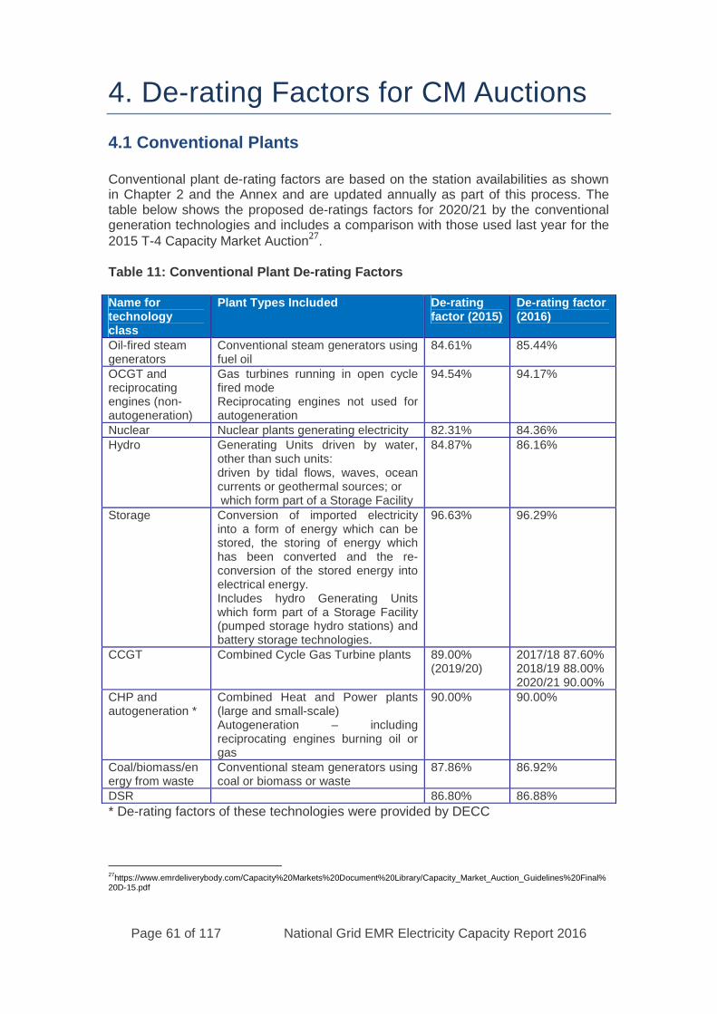
Page 61 of 117 National Grid EMR Electricity Capacity Report 2016
4. De-rating Factors for CM Auctions
4.1 Conventional Plants
Conventional plant de-rating factors are based on the station availabilities as shownin Chapter 2 and the Annex and are updated annually as part of this process. Thetable below shows the proposed de-ratings factors for 2020/21 by the conventionalgeneration technologies and includes a comparison with those used last year for the2015 T-4 Capacity Market Auction
27.
Table 11: Conventional Plant De-rating Factors
Name fortechnologyclass
Plant Types Included De-ratingfactor (2015)
De-rating factor(2016)
Oil-fired steamgenerators
Conventional steam generators usingfuel oil
84.61% 85.44%
OCGT andreciprocatingengines (non-autogeneration)
Gas turbines running in open cyclefired modeReciprocating engines not used forautogeneration
94.54% 94.17%
Nuclear Nuclear plants generating electricity 82.31% 84.36%Hydro Generating Units driven by water,
other than such units:driven by tidal flows, waves, oceancurrents or geothermal sources; orwhich form part of a Storage Facility
84.87% 86.16%
Storage Conversion of imported electricityinto a form of energy which can bestored, the storing of energy whichhas been converted and the re-conversion of the stored energy intoelectrical energy.Includes hydro Generating Unitswhich form part of a Storage Facility(pumped storage hydro stations) andbattery storage technologies.
96.63% 96.29%
CCGT Combined Cycle Gas Turbine plants 89.00%(2019/20)
2017/18 87.60%2018/19 88.00%2020/21 90.00%
CHP andautogeneration *
Combined Heat and Power plants(large and small-scale)Autogeneration – includingreciprocating engines burning oil orgas
90.00% 90.00%
Coal/biomass/energy from waste
Conventional steam generators usingcoal or biomass or waste
87.86% 86.92%
DSR 86.80% 86.88%
* De-rating factors of these technologies were provided by DECC
27https://www.emrdeliverybody.com/Capacity%20Markets%20Document%20Library/Capacity_Market_Auction_Guidelines%20Final%
20D-15.pdf
Page 62 of 117 National Grid EMR Electricity Capacity Report 2016
4.2 DSR De-rating Factor
The De-rating factor for DSR CMUs is the Average Availability of Non-BSC BalancingServices (“AABS”)
It is calculated by determining the mean average of the declared availabilitiesof all Non-BSC Balancing Services providers at real time in High DemandSettlement Periods over the three immediately preceding Core WinterPeriods, divided by their contracted volumes.
Short Term Operating Reserve (STOR) availability was chosen as a basis forthese calculations as this is the largest, most accurate and relevant data setavailable to National Grid. Availability information following settlement alsoincludes the effect of any utilisation failure, so this provides a more accurateview than declared availability. Note there is a low volume of other applicableBalancing Services data available such as FCDM (Frequency ControlDemand Management) and FFR services (Firm Frequency Response) butthese services are either not comparable to Capacity Market data, or the datais not sufficient to add value to the process.
Only Committed STOR units, where a service provider must make the serviceavailable for all availability windows within the contracted season, wereconsidered and used in the calculation. The availability of Flexible units isfound to be low due to the nature of the load and hence the reason for theflexible service. When including Flexible STOR the de-rating factor wasshown to decrease so was not used. The committed service also moreclosely reflects the capacity product than the other services. Currentlycontracted unit data was used as this reflects the current market rather thanunits that may have left the market due to low performance.
The following explains the methodology used to calculate the DSR De-ratingfigure (using Committed STOR availability over the most recent 3 winters at50th percentile demand):
1. The mean average of the declared availabilities:- The mean average of the STOR available volume or zero if not available,where the volume is as settled including any deemed unavailability followingan Event of Default, for the defined STOR units in the defined settlementperiods.- Units that have declared themselves unavailable will have zero availabilityfor the relevant period.- As per the STOR Standard Contract terms, units that have failed to deliverby the end of their defined response time following a utilisation instruction(<90% of expected volume in response time) will have zero availability for theperiods impacted.- Units that have delivered <90% expected volume for an instruction will havezero availability for the remainder of the window.- Units that have baseline generation/load at level other than agreed i.e. if agenerator metering >0MW, if a demand unit, metering < Contracted MW, willhave zero availability for the entire window.
2. Of all Non-BSC Balancing Services: Non-BM Committed STOR units thatwere contracted for the latest winter season.
Page 63 of 117 National Grid EMR Electricity Capacity Report 2016
3. Over the High Demand Settlement Periods: Settlement Periods insidedefined STOR windows between 7 am and 7pm where the GB peak demandfor the day was greater than the 50th percentile of demands for that winter(November to March).
4. For the three immediately preceding Core Winter Periods: on week daysbetween December and February.
5. Divided by their contracted volumes: settlement period STOR contractvolume.
4.3 Interconnectors
As part of the UK’s State aid approval for the Capacity Market, interconnectors havebeen eligible to participate in the CM since the 2015 auction. As such, the UK hascommitted to include interconnectors in the 2017/18 early auction. The future ofpotential flows through interconnectors is very uncertain and as a consequence thereis no one answer to the question of what can be assumed to flow through theinterconnectors at times of system stress. This section outlines the variousapproaches National Grid, in agreement with DECC, has considered in determiningan appropriate de-rating factor range for the Secretary of State to then decide thefactors to apply to interconnectors in the 2017/18 early auction and 2020/21 T-4auction.
4.3.1 Methodology
We commissioned Baringa to model flows between GB and connected countries foreach scenario using their pan-European market model. Flows from November toFebruary were modelled for each scenario based on FES 2015 demand andgeneration data, FES 2016 electricity interconnector capacity, and Baringa’s owndataset for non-GB countries. This year’s analysis has been enhanced incorporatingrecommendations from the PTE. The enhancements are:
Scarcity premia modelled Demand history increased to 9 years (2006 to 2014) correlated across
Europe and with wind generation Larger number of simulations
The modelling assumed that I-SEM would go live in October 2017 removing theincentive for flows from GB to Ireland during the peak winter hours. Ireland wasmodelled as a single price area so Ireland’s North/South constraint had no impact.
All hours with a GB capacity margin less than or equal to zero, from the modelsimulation, were selected to represent times when imports were required. Theaverage flow as a percentage of capacity was calculated for each connected countryand FES scenario. The average value across all four scenarios sets the top of therecommended range of de-rating factors. Percentiles of the distribution of thesesimulations were calculated to assess the variability in flows.
DECC commissioned Pöyry to update their analysis of historical de-rating factorsused to inform last year’s ranges. In all cases these set the bottom of the
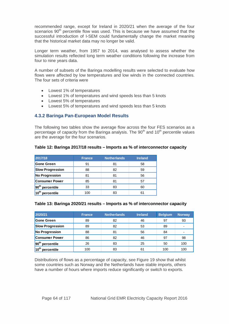
Page 64 of 117 National Grid EMR Electricity Capacity Report 2016
recommended range, except for Ireland in 2020/21 when the average of the fourscenarios 90th percentile flow was used. This is because we have assumed that thesuccessful introduction of I-SEM could fundamentally change the market meaningthat the historical market data may no longer be valid.
Longer term weather, from 1957 to 2014, was analysed to assess whether thesimulation results reflected long term weather conditions following the increase fromfour to nine years data.
A number of subsets of the Baringa modelling results were selected to evaluate howflows were affected by low temperatures and low winds in the connected countries.The four sets of criteria were
Lowest 1% of temperatures Lowest 1% of temperatures and wind speeds less than 5 knots Lowest 5% of temperatures Lowest 5% of temperatures and wind speeds less than 5 knots
4.3.2 Baringa Pan-European Model Results
The following two tables show the average flow across the four FES scenarios as apercentage of capacity from the Baringa analysis. The 90th and 10th percentile valuesare the average for the four scenarios.
Table 12: Baringa 2017/18 results – Imports as % of interconnector capacity
Table 13: Baringa 2020/21 results – Imports as % of interconnector capacity
Distributions of flows as a percentage of capacity, see Figure 19 show that whilstsome countries such as Norway and the Netherlands have stable imports, othershave a number of hours where imports reduce significantly or switch to exports.
2017/18 France Netherlands Ireland
Gone Green 91 81 58
Slow Progression 88 82 59
No Progression 81 81 56
Consumer Power 85 81 57
90th
percentile 33 83 60
10th
percentile 100 83 61
2020/21 France Netherlands Ireland Belgium Norway
Gone Green 89 82 46 97 93
Slow Progression 89 82 53 89 -
No Progression 88 81 56 84 -
Consumer Power 86 82 46 97 98
90th
percentile 26 83 25 50 100
10th
percentile 100 83 61 100 100
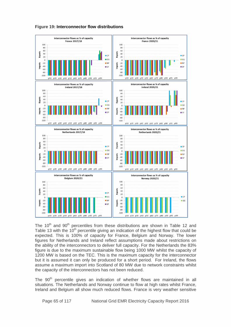
Page 65 of 117 National Grid EMR Electricity Capacity Report 2016
Figure 19: Interconnector flow distributions
The 10th and 90th percentiles from these distributions are shown in Table 12 andTable 13 with the 10th percentile giving an indication of the highest flow that could beexpected. This is 100% of capacity for France, Belgium and Norway. The lowerfigures for Netherlands and Ireland reflect assumptions made about restrictions onthe ability of the interconnectors to deliver full capacity. For the Netherlands the 83%figure is due to the maximum sustainable flow being 1000 MW whilst the capacity of1200 MW is based on the TEC. This is the maximum capacity for the interconnectorbut it is assumed it can only be produced for a short period. For Ireland, the flowsassume a maximum import into Scotland of 80 MW due to network constraints whilstthe capacity of the interconnectors has not been reduced.
The 90th percentile gives an indication of whether flows are maintained in allsituations. The Netherlands and Norway continue to flow at high rates whilst France,Ireland and Belgium all show much reduced flows. France is very weather sensitive

Page 66 of 117 National Grid EMR Electricity Capacity Report 2016
with a need for large net imports at high demand levels so the availability of importsfrom France is reduced when stress conditions coincide. As Ireland has a highproportion of wind generation its ability to export to GB depends on stress periods inIreland, caused by low wind and high demand, not coinciding with GB’s need forimports. Belgium is reliant on its nuclear power stations remaining operational.
4.3.3 Validation/ Comparison/Other Analysis
One concern with the analysis in 2015 was that there were only four historical yearsin the pan-European modelling. This year’s analysis increases the number ofhistorical years to nine (2006 to 2014). Comparing the temperature distributions forthese nine years with all years from 1957 produces small differences, as illustrated inFigure 20 but when these differences are used to scale the interconnector flows torepresent the longer time period the impact on mean flow percentages is minimal sono scaling to long term weather has been applied. Further analysis may identify ifthere are significant differences in extreme events but this will require a detailedproject which cannot be undertaken in time so will be considered as a developmentproject for next year.
Figure 20: Temperature distributions

Page 67 of 117 National Grid EMR Electricity Capacity Report 2016
4.3.4 Pöyry historical analysis
DECC commissioned Pöyry to update their analysis of historical flows. The historicaldata used was the top 50% of peak demand periods during the winter quarter, 7amto 7pm business days from 2009 to 2015. For the existing interconnectors theaverage de-rating factors are calculated for those periods where the price differentialwas positive and the interconnector was importing to GB. For new interconnectorsthe factors are calculated from the percentage of periods with a positive pricedifferential. In recent years interconnector flows have become more consistent withprice differentials. The main exception is Ireland where the relationship between flowdirection and prices remains poor.
For this analysis two sets of data are shown. The Pöyry report calculates the averagefor the last seven years. This sets the floor for the de-rating factors. In addition wehave also calculated the average of the last four years to reflect changes in themarket coupled era. However, the longer period represents a wider range of eventsand risks rather than just price. Examples of such events include droughts in Norwaywhich are better reflected by the longer period. Figure 21 shows the efficiency ofinterconnector flows measured as the percentage of time interconnector imports toGB are in line with positive price differentials. Ireland is expected to remain low untilthe introduction of I-SEM in October 2017. Table 14 compares the historical de-ratingfactors based on the seven year and four year historical averages.
Figure 21: Efficiency of interconnector flows
Table 14: Historical de-rating factors
% France Netherlands Ireland Belgium Norway
2009-2015 45 70 2 65 76
2012-2015 67 76 4 76 92
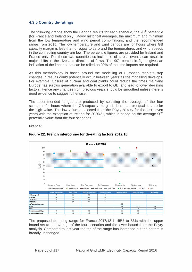
Page 68 of 117 National Grid EMR Electricity Capacity Report 2016
4.3.5 Country de-ratings
The following graphs show the Baringa results for each scenario, the 90th percentile(for France and Ireland only), Pöyry historical averages, the maximum and minimumfrom the low temperature and wind period combinations, and the recommendedrange from 2015. The low temperature and wind periods are for hours where GBcapacity margin is less than or equal to zero and the temperatures and wind speedsin the connecting country are low. The percentile figures are provided for Ireland andFrance only. For these two countries co-incidence of stress events can result inmajor shifts in the size and direction of flows. The 90th percentile figure gives anindication of the imports that can be relied on 90% of the time imports are required.
As this methodology is based around the modelling of European markets stepchanges in results could potentially occur between years as the modelling develops.For example, closure of nuclear and coal plants could reduce the times mainlandEurope has surplus generation available to export to GB, and lead to lower de-ratingfactors. Hence any changes from previous years should be smoothed unless there isgood evidence to suggest otherwise.
The recommended ranges are produced by selecting the average of the fourscenarios for hours where the GB capacity margin is less than or equal to zero forthe high value. The low value is selected from the Pöyry history for the last sevenyears with the exception of Ireland for 2020/21, which is based on the average 90th
percentile value from the four scenarios.
France:
Figure 22: French interconnector de-rating factors 2017/18
The proposed de-rating range for France 2017/18 is 45% to 86% with the upperbound set to the average of the four scenarios and the lower bound from the Pöyryanalysis. Compared to last year the top of the range has increased but the bottom isbroadly unchanged.
Consumer Power Gone Green Slow Progression No Progression 90th percentile Weather range 2015 range
GB margin<0 85 91 88 81
Average 86 86 86 86
2009-2015 45 45 45 45
2012-2015 67 67 67 67
90th percentile average 33
High 100 100 70
Low 0 70 50
Recommended High 86 86 86 86 86 86
Recommended Low 45 45 45 45 45 45
0
10
20
30
40
50
60
70
80
90
100
Consumer Power Gone Green Slow Progression No Progression 90th percentile Weather range 2015 range
De-
rati
ng
facto
r
France 2017/18
Recommended range GB margin<0 Average 2009-2015 2012-2015 90th percentile average High Low
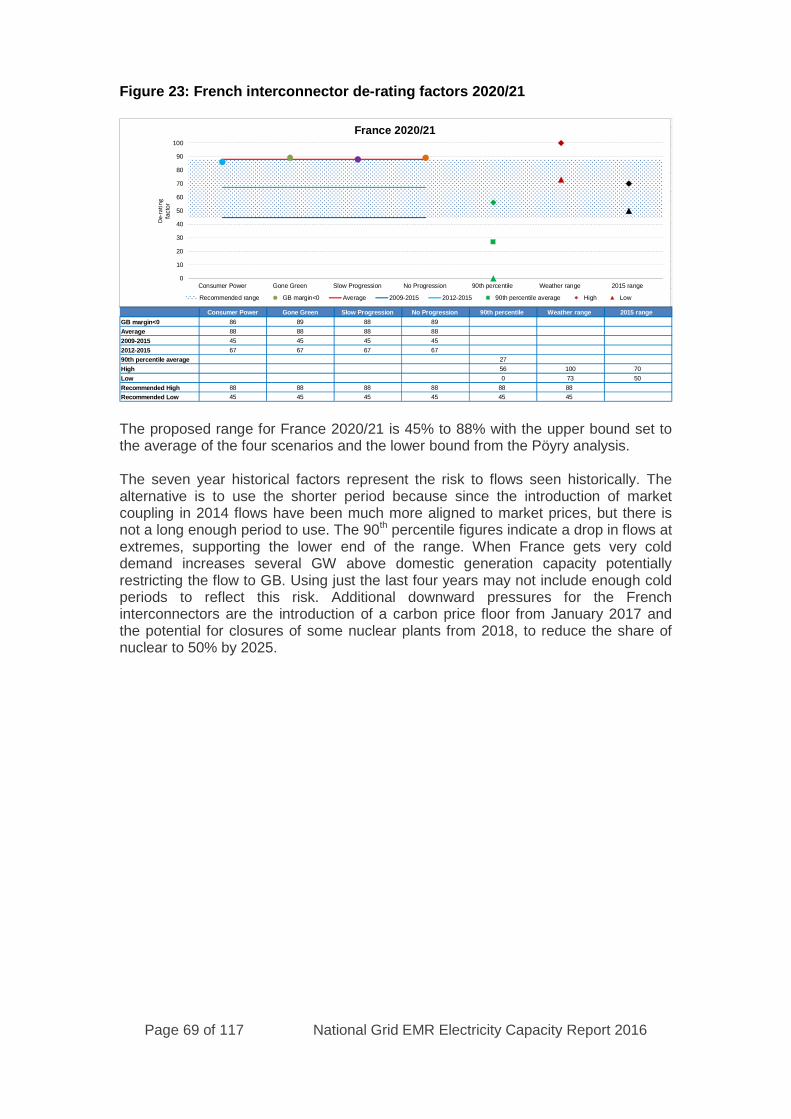
Page 69 of 117 National Grid EMR Electricity Capacity Report 2016
Figure 23: French interconnector de-rating factors 2020/21
The proposed range for France 2020/21 is 45% to 88% with the upper bound set tothe average of the four scenarios and the lower bound from the Pöyry analysis.
The seven year historical factors represent the risk to flows seen historically. Thealternative is to use the shorter period because since the introduction of marketcoupling in 2014 flows have been much more aligned to market prices, but there isnot a long enough period to use. The 90th percentile figures indicate a drop in flows atextremes, supporting the lower end of the range. When France gets very colddemand increases several GW above domestic generation capacity potentiallyrestricting the flow to GB. Using just the last four years may not include enough coldperiods to reflect this risk. Additional downward pressures for the Frenchinterconnectors are the introduction of a carbon price floor from January 2017 andthe potential for closures of some nuclear plants from 2018, to reduce the share ofnuclear to 50% by 2025.
Consumer Power Gone Green Slow Progression No Progression 90th percentile Weather range 2015 range
GB margin<0 86 89 88 89
Average 88 88 88 88
2009-2015 45 45 45 45
2012-2015 67 67 67 67
90th percentile average 27
High 56 100 70
Low 0 73 50
Recommended High 88 88 88 88 88 88
Recommended Low 45 45 45 45 45 45
0
10
20
30
40
50
60
70
80
90
100
Consumer Power Gone Green Slow Progression No Progression 90th percentile Weather range 2015 range
De-
rati
ng
facto
r
France 2020/21
Recommended range GB margin<0 Average 2009-2015 2012-2015 90th percentile average High Low
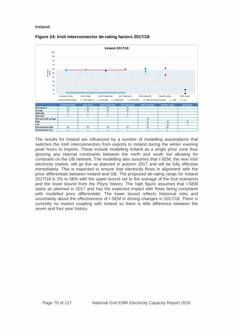
Page 70 of 117 National Grid EMR Electricity Capacity Report 2016
Ireland:
Figure 24: Irish interconnector de-rating factors 2017/18
The results for Ireland are influenced by a number of modelling assumptions thatswitches the Irish interconnectors from exports to Ireland during the winter eveningpeak hours to imports. These include modelling Ireland as a single price zone thusignoring any internal constraints between the north and south but allowing forconstraint on the GB network. The modelling also assumes that I-SEM, the new Irishelectricity market, will go live as planned in autumn 2017 and will be fully effectiveimmediately. This is expected to ensure that electricity flows in alignment with theprice differentials between Ireland and GB. The proposed de-rating range for Ireland2017/18 is 2% to 58% with the upper bound set to the average of the four scenariosand the lower bound from the Pöyry history. The high figure assumes that I-SEMstarts as planned in 2017 and has the expected impact with flows being consistentwith modelled price differentials. The lower bound reflects historical risks anduncertainty about the effectiveness of I-SEM in driving changes in 2017/18. There iscurrently no market coupling with Ireland so there is little difference between theseven and four year history.
Consumer Power Gone Green Slow Progression No Progression 90th percentile Weather range 2015 range
GB margin<0 57 58 56 59
Average 58 58 58 58
2009-2015 2 2 2 2
2012-2015 4 4 4 4
90th percentile average 59
High 61 61 10
Low 54 46 2
Recommended High 58 58 58 58 58 58
Recommended Low 2 2 2 2 2 2
0
10
20
30
40
50
60
70
80
90
100
Consumer Power Gone Green Slow Progression No Progression 90th percentile Weather range 2015 range
De-
rati
ng
facto
rIreland 2017/18
Recommended range GB margin<0 Average 2009-2015 2012-2015 90th percentile average High Low
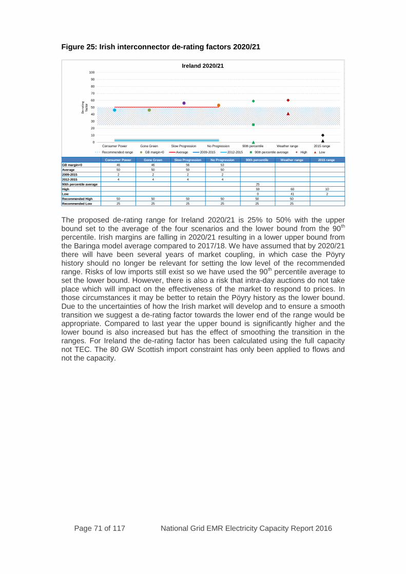
Page 71 of 117 National Grid EMR Electricity Capacity Report 2016
Figure 25: Irish interconnector de-rating factors 2020/21
The proposed de-rating range for Ireland 2020/21 is 25% to 50% with the upperbound set to the average of the four scenarios and the lower bound from the 90th
percentile. Irish margins are falling in 2020/21 resulting in a lower upper bound fromthe Baringa model average compared to 2017/18. We have assumed that by 2020/21there will have been several years of market coupling, in which case the Pöyryhistory should no longer be relevant for setting the low level of the recommendedrange. Risks of low imports still exist so we have used the 90th percentile average toset the lower bound. However, there is also a risk that intra-day auctions do not takeplace which will impact on the effectiveness of the market to respond to prices. Inthose circumstances it may be better to retain the Pöyry history as the lower bound.Due to the uncertainties of how the Irish market will develop and to ensure a smoothtransition we suggest a de-rating factor towards the lower end of the range would beappropriate. Compared to last year the upper bound is significantly higher and thelower bound is also increased but has the effect of smoothing the transition in theranges. For Ireland the de-rating factor has been calculated using the full capacitynot TEC. The 80 GW Scottish import constraint has only been applied to flows andnot the capacity.
41
45
54
52
Consumer Power Gone Green Slow Progression No Progression 90th percentile Weather range 2015 range
GB margin<0 46 46 56 53
Average 50 50 50 50
2009-2015 2 2 2 2
2012-2015 4 4 4 4
90th percentile average 25
High 59 60 10
Low 0 41 2
Recommended High 50 50 50 50 50 50
Recommended Low 25 25 25 25 25 25
0
10
20
30
40
50
60
70
80
90
100
Consumer Power Gone Green Slow Progression No Progression 90th percentile Weather range 2015 range
De-
rati
ng
facto
r
Ireland 2020/21
Recommended range GB margin<0 Average 2009-2015 2012-2015 90th percentile average High Low
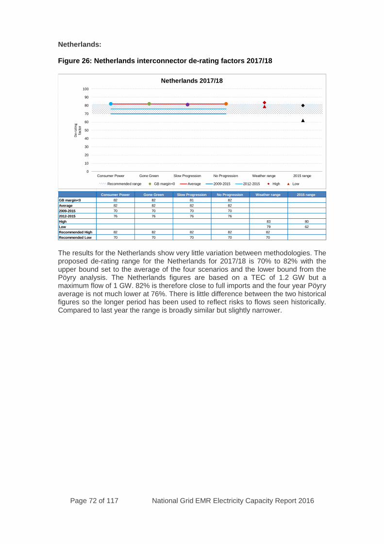
Page 72 of 117 National Grid EMR Electricity Capacity Report 2016
Netherlands:
Figure 26: Netherlands interconnector de-rating factors 2017/18
The results for the Netherlands show very little variation between methodologies. Theproposed de-rating range for the Netherlands for 2017/18 is 70% to 82% with theupper bound set to the average of the four scenarios and the lower bound from thePöyry analysis. The Netherlands figures are based on a TEC of 1.2 GW but amaximum flow of 1 GW. 82% is therefore close to full imports and the four year Pöyryaverage is not much lower at 76%. There is little difference between the two historicalfigures so the longer period has been used to reflect risks to flows seen historically.Compared to last year the range is broadly similar but slightly narrower.
Consumer Power Gone Green Slow Progression No Progression Weather range 2015 range
GB margin<0 82 82 81 82
Average 82 82 82 82
2009-2015 70 70 70 70
2012-2015 76 76 76 76
High 83 80
Low 79 62
Recommended High 82 82 82 82 82
Recommended Low 70 70 70 70 70
0
10
20
30
40
50
60
70
80
90
100
Consumer Power Gone Green Slow Progression No Progression Weather range 2015 range
De-
rati
ng
facto
rNetherlands 2017/18
Recommended range GB margin<0 Average 2009-2015 2012-2015 High Low
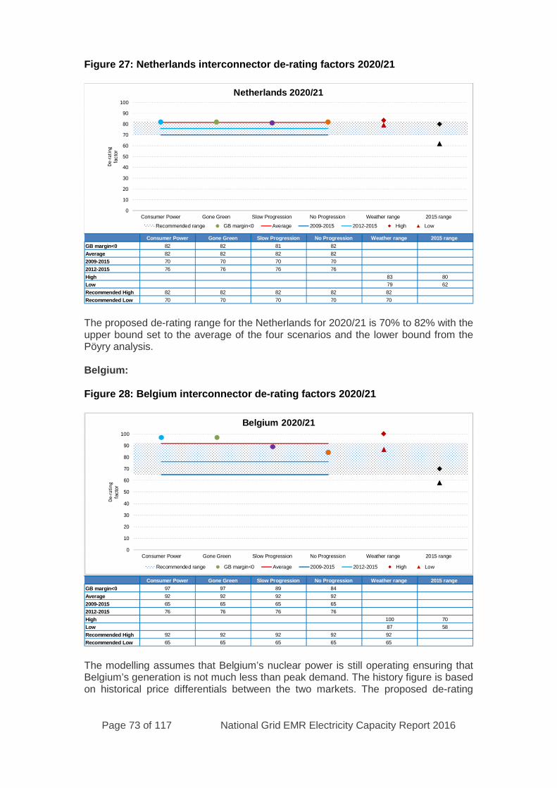
Page 73 of 117 National Grid EMR Electricity Capacity Report 2016
Figure 27: Netherlands interconnector de-rating factors 2020/21
The proposed de-rating range for the Netherlands for 2020/21 is 70% to 82% with theupper bound set to the average of the four scenarios and the lower bound from thePöyry analysis.
Belgium:
Figure 28: Belgium interconnector de-rating factors 2020/21
The modelling assumes that Belgium’s nuclear power is still operating ensuring thatBelgium’s generation is not much less than peak demand. The history figure is basedon historical price differentials between the two markets. The proposed de-rating
Consumer Power Gone Green Slow Progression No Progression Weather range 2015 range
GB margin<0 82 82 81 82
Average 82 82 82 82
2009-2015 70 70 70 70
2012-2015 76 76 76 76
High 83 80
Low 79 62
Recommended High 82 82 82 82 82
Recommended Low 70 70 70 70 70
0
10
20
30
40
50
60
70
80
90
100
Consumer Power Gone Green Slow Progression No Progression Weather range 2015 range
De-
rati
ng
facto
r
Netherlands 2020/21
Recommended range GB margin<0 Average 2009-2015 2012-2015 High Low
Consumer Power Gone Green Slow Progression No Progression Weather range 2015 range
GB margin<0 97 97 89 84
Average 92 92 92 92
2009-2015 65 65 65 65
2012-2015 76 76 76 76
High 100 70
Low 87 58
Recommended High 92 92 92 92 92
Recommended Low 65 65 65 65 65
0
10
20
30
40
50
60
70
80
90
100
Consumer Power Gone Green Slow Progression No Progression Weather range 2015 range
De-
rati
ng
facto
r
Belgium 2020/21
Recommended range GB margin<0 Average 2009-2015 2012-2015 High Low

Page 74 of 117 National Grid EMR Electricity Capacity Report 2016
range for Belgium for 2020/21 is 65% to 92% with the upper bound set to theaverage of the four scenarios and the lower bound from the Pöyry analysis. Thelonger history is used for the lower bound to reflect risks to flows seen historically.The alternative is to use a shorter historical period based on market coupling beingintroduced across Europe but as market coupling did not go live for Great Britain until2014 there is not a long enough period to use. Compared to last year the range iswider and higher. This range could be reduced to reflect lower availability duringcommissioning.
Norway:
Figure 29: Norway interconnector de-rating factors 2020/21
Norway only features in Consumer Power and Gone Green and was not part of the2015 analysis for the 2019/20 auction. The history figure is based on historical pricedifferentials between the two markets. The proposed de-rating range for Norway for2020/21 is 76% to 96% with the upper bound set to the average of the four scenariosand the lower bound from the Pöyry analysis. (The impact of market coupling on thePöyry figure is not relevant for Norway because there is not an existing link.) A keydriver of Norwegian prices is the level of water in the reservoirs. A longer period ofhistory ensures a greater range of weather events are represented so for Norway theseven year history should set the bottom of the range and the four year history isn’tconsidered as an appropriate alternative.
Summary
Table 15 shows the recommended ranges for de-rating factors in 2017/18 and2020/21 for all existing and potential interconnected countries. Note that there are nopotential ranges for interconnector de-rating factors for 2018/19 as they are excludedfrom participating in the auctions for that delivery year.
These de-rating factors are based around the modelling undertaken by Baringa usingtheir pan-European market model and Pöyry’s analysis on historical performance.The top of the de-rating factor ranges are set by the Baringa modelling with Pöyry’sanalysis of seven historical years setting the bottom of the ranges for all but Ireland in2020/21. We have assumed that by 2020/21 the successful introduction of I-SEM
Consumer Power Gone Green Slow Progression No Progression Weather range 2015 range
GB margin<0 98 93
Average 96 96
2009-2015 76 76
2012-2015 92 92
High 100
Low 89
Recommended High 96 96 96 96 96
Recommended Low 76 76 76 76 76
0
10
20
30
40
50
60
70
80
90
100
Consumer Power Gone Green Slow Progression No Progression Weather range 2015 range
De-
rati
ngfa
ctor
Norway 2020/21
Recommended range GB margin<0 Average 2009-2015 2012-2015 High Low
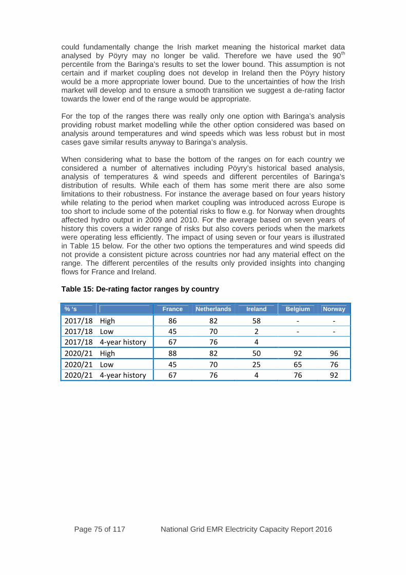
Page 75 of 117 National Grid EMR Electricity Capacity Report 2016
could fundamentally change the Irish market meaning the historical market dataanalysed by Pöyry may no longer be valid. Therefore we have used the 90th
percentile from the Baringa’s results to set the lower bound. This assumption is notcertain and if market coupling does not develop in Ireland then the Pöyry historywould be a more appropriate lower bound. Due to the uncertainties of how the Irishmarket will develop and to ensure a smooth transition we suggest a de-rating factortowards the lower end of the range would be appropriate.
For the top of the ranges there was really only one option with Baringa’s analysisproviding robust market modelling while the other option considered was based onanalysis around temperatures and wind speeds which was less robust but in mostcases gave similar results anyway to Baringa’s analysis.
When considering what to base the bottom of the ranges on for each country weconsidered a number of alternatives including Pöyry’s historical based analysis,analysis of temperatures & wind speeds and different percentiles of Baringa’sdistribution of results. While each of them has some merit there are also somelimitations to their robustness. For instance the average based on four years historywhile relating to the period when market coupling was introduced across Europe istoo short to include some of the potential risks to flow e.g. for Norway when droughtsaffected hydro output in 2009 and 2010. For the average based on seven years ofhistory this covers a wider range of risks but also covers periods when the marketswere operating less efficiently. The impact of using seven or four years is illustratedin Table 15 below. For the other two options the temperatures and wind speeds didnot provide a consistent picture across countries nor had any material effect on therange. The different percentiles of the results only provided insights into changingflows for France and Ireland.
Table 15: De-rating factor ranges by country
% ‘s France Netherlands Ireland Belgium Norway
2017/18 High 86 82 58 - -
2017/18 Low 45 70 2 - -
2017/18 4-year history 67 76 4
2020/21 High 88 82 50 92 96
2020/21 Low 45 70 25 65 76
2020/21 4-year history 67 76 4 76 92

Page 76 of 117 National Grid EMR Electricity Capacity Report 2016
5. Results and Recommendation for2020/21 T-4 Auction
This chapter presents the results for 2020/21 only from the modelling of thescenarios and sensitivities relevant to 2020/21. Results for 2017/18 and 2018/19 canbe found in chapters 6 and 7 respectively. Further information on capacityrequirements in years out to 2030/31 can be found in section 3.11.
5.1 Sensitivities to model
The analysis assumes that the FES scenarios will cover uncertainty by incorporatingranges for annual and peak demand, DSR, interconnection and generation with thesensitivities covering uncertainty in single variables. Chapter 3 describes thescenarios and sensitivities modelled for the 2016 ECR. The agreed sensitivities tomodel for 2020/21 cover non-delivery, weather, plant availability and demand:
Low Wind Output at times of cold weather (LOW WIND) High Wind Output at times of cold weather (HIGH WIND) Weather Cold Winter (COLD) Weather Warm Winter (WARM) High Plant Availabilities (HIGH AVAIL) Low Plant Availabilities (LOW AVAIL) High Demand (HIGH DEMAND) Low Demand (LOW DEMAND) Non Delivery (NON DEL): 9 sensitivities in 400 MW increments up to 3600
MW.
5.2 Results
The following table shows the modelling results sorted in order of de-rated capacityrequired to meet the 3 hours LOLE Reliability Standard. It also shows the capacityoutside of the CM (including previously contracted capacity assumed for each case),the total de-rated capacity and ACS peak demand.
The Base Case also assumes that some capacity contracted for 2020/21 in previousT-4 auctions is not able to honour its awarded contracts whereas the DECC scenarioassumes all previously contracted capacity honours its contracts.
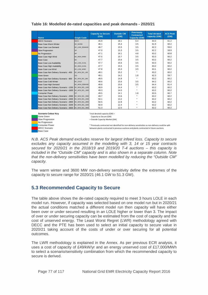
Page 77 of 117 National Grid EMR Electricity Capacity Report 2016
Table 16: Modelled de-rated capacities and peak demands - 2020/21
N.B. ACS Peak demand excludes reserve for largest infeed loss. Capacity to secureexcludes any capacity assumed in the modelling with 3, 14 or 15 year contractssecured for 2020/21 in the 2018/19 and 2019/20 T-4 auctions – this capacity isincluded in the “Outside CM” capacity and is also shown in a separate column. Notethat the non-delivery sensitivities have been modelled by reducing the “Outside CM”capacity.
The warm winter and 3600 MW non-delivery sensitivity define the extremes of thecapacity to secure range for 2020/21 (46.1 GW to 51.3 GW).
5.3 Recommended Capacity to Secure
The table above shows the de-rated capacity required to meet 3 hours LOLE in eachmodel run. However, if capacity was selected based on one model run but in 2020/21the actual conditions matched a different model run then capacity will have eitherbeen over or under secured resulting in an LOLE higher or lower than 3. The impactof over or under securing capacity can be estimated from the cost of capacity and thecost of unserved energy. The Least Worst Regret (LWR) methodology agreed withDECC and the PTE has been used to select an initial capacity to secure value in2020/21 taking account of the costs of under or over securing for all potentialoutcomes.
The LWR methodology is explained in the Annex. As per previous ECR analysis, ituses a cost of capacity of £49/kW/yr and an energy unserved cost of £17,000/MWhto select a scenario/sensitivity combination from which the recommended capacity tosecure is derived.
Name Graph Code
Capacity to Secure
(GW)
Outside CM
(GW)
Previously
Contracted
Capacity (GW)
Total derated
capacity (GW)
ACS Peak
(GW)
DECC Scenario DECC 45.9 18.1 6.4 64.0 61.2
Base Case Warm Winter BC_WARM 46.1 15.4 3.5 61.5 60.2
Base Case Low Demand BC_LOW_DEMAND 46.7 15.5 3.5 62.2 59.0
Slow Progression SP 47.0 15.3 3.5 62.2 59.9
No Progression NP 47.1 16.1 4.8 63.2 60.8
Base Case High Wind BC_HIGH_WIND 47.5 15.7 3.5 63.3 60.2
Base Case BC 47.7 15.6 3.5 63.2 60.2
Base Case Low Availability BC_LOW_AVAIL 47.7 15.6 3.5 63.3 60.2
Base Case High Availability BC_HIGH_AVAIL 47.7 15.5 3.5 63.2 60.2
Base Case Low Wind BC_LOW_WIND 47.8 15.3 3.5 63.1 60.2
Base Case Non Delivery Scenario: -400 BC_NON_DEL_400 48.1 15.2 * 63.2 60.2
Gone Green GG 48.1 14.2 1.8 62.3 59.7
Base Case Non Delivery Scenario: -800 BC_NON_DEL_800 48.5 14.8 * 63.2 60.2
Base Case Cold Winter BC_COLD 48.6 15.6 3.5 64.2 60.2
Base Case High Demand BC_HIGH_DEMAND 48.8 15.6 3.5 64.4 61.4
Base Case Non Delivery Scenario: -1200 BC_NON_DEL_1200 48.9 14.4 * 63.2 60.2
Base Case Non Delivery Scenario: -1600 BC_NON_DEL_1600 49.3 14.0 * 63.2 60.2
Consumer Power CP 49.5 14.1 1.8 63.5 60.7
Base Case Non Delivery Scenario: -2000 BC_NON_DEL_2000 49.7 13.6 * 63.2 60.2
Base Case Non Delivery Scenario: -2400 BC_NON_DEL_2400 50.1 13.2 * 63.2 60.2
Base Case Non Delivery Scenario: -2800 BC_NON_DEL_2800 50.5 12.8 * 63.2 60.2
Base Case Non Delivery Scenario: -3200 BC_NON_DEL_3200 50.9 12.4 * 63.2 60.2
Base Case Non Delivery Scenario: -3600 BC_NON_DEL_3600 51.3 12.0 * 63.2 60.2
Scenario Colour Key Total derated capacity (GW) =
Gone Green Capacity to Secure (GW)
Slow Progression + Outside Capacity Market (GW)
No Progression
Consumer Power * Previously contracted not identified for non-delivery sensitivities as non-delivery could be split
DECC Scenario between plants contracted in previous auctions and plants contracted in future auctions.
Base Case

Page 78 of 117 National Grid EMR Electricity Capacity Report 2016
The outcome of the Least Worst Regret calculation applied to all of National Grid’sscenarios and sensitivities is an initial capacity to secure for 2020/21 of 49.5 GW(49.48 GW before rounding) based on the Consumer Power scenario. As this is aFES scenario, a small adjustment is required to bring it into line with the DFAIncentive by selecting the nearest Base Case sensitivity based on the DFA Incentivedemand level (as per section 2.6.3). In this case the nearest sensitivity is the 2000MW non-delivery sensitivity (49.65 GW before rounding) that is marginally closerthan the 1600 MW non-delivery sensitivity (49.25 GW before rounding).
This leads to a recommended capacity to secure for 2020/21 of 49.7 GW derivedfrom the requirement of the Base Case 2000MW non-delivery sensitivity. This doesnot take account of a different clearing price to net CONE resulting from the auctionas our recommended target capacity to secure corresponds to the value on the CMdemand curve for the net CONE capacity cost. It also excludes any capacity securedin earlier auctions for 2020/21 that is assumed in the Base Case
In general, when compared to the analysis for 2019/20 in the 2015 ECR, the 2016scenarios and sensitivities for 2020/21 contain higher levels of CM-ineligible de-ratedcapacity at peak due to higher contribution from renewables (see Annex forbreakdown), in part due to the new offshore power curve, as well as higher levels ofassumed ineligible autogeneration below 2 MW28. However the reduction in totalCM-eligible capacity requirement due to higher levels of ineligible capacity is offsetby using a wider range of non-delivery sensitivities that increases the requirement inthe LWR analysis. The warm winter sensitivity is the key to the LWR result as it is thesensitivity that sets the highest regret cost for the recommended capacity level (seeAnnex for more details on how regret costs are determined in the LWR calculation).
The following chart illustrates the full range of potential capacity levels (from NationalGrid scenarios and sensitivities) plus the DECC scenario and identifies the LeastWorst Regret recommended capacity. Individual scenarios are highlighted with largermarkers and each scenario and sensitivity is colour coded. Note that National Grid’srecommendation concentrates on the target capacity alone.
28Note that unsupported capacity under 2 MW can enter the auction if it is combined with other capacity by an aggregator to give a
total above 2 MW
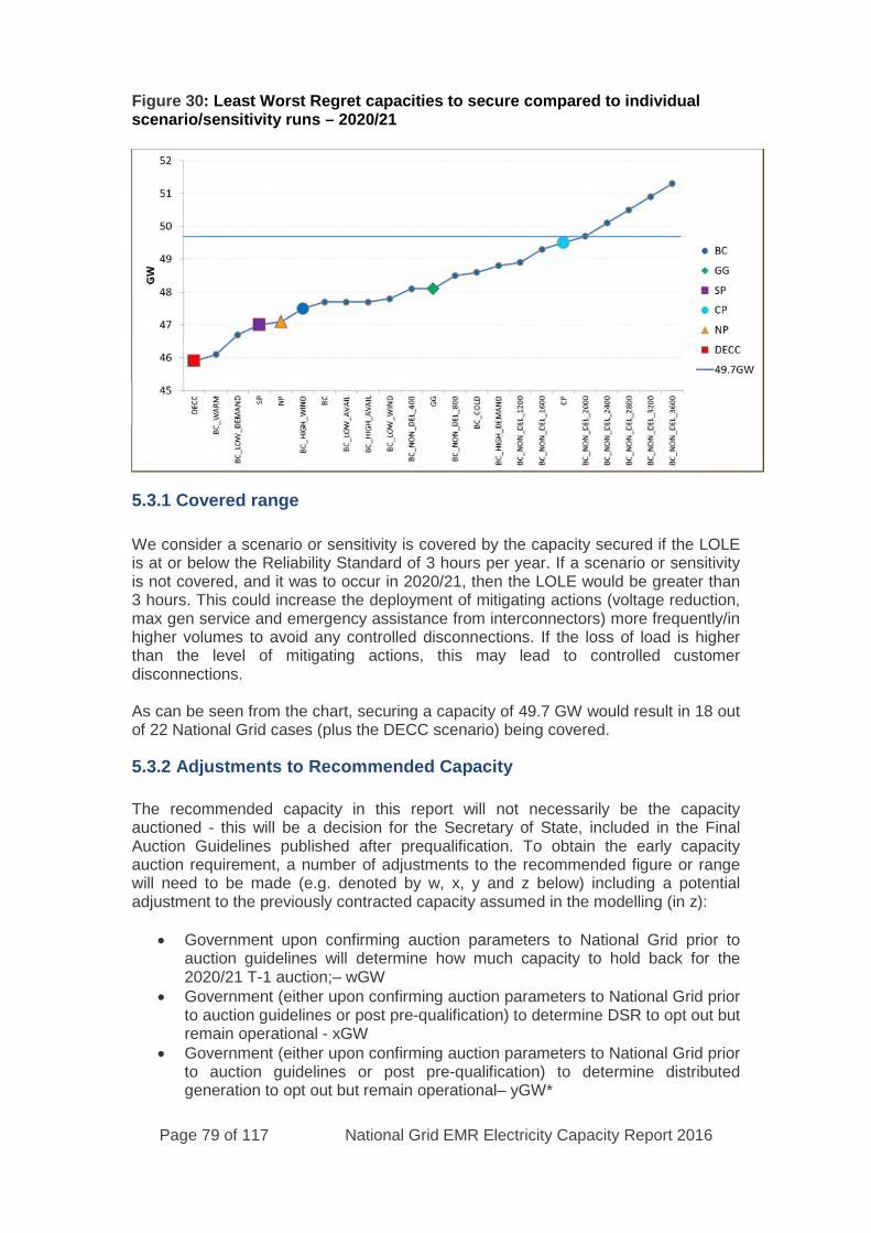
Page 79 of 117 National Grid EMR Electricity Capacity Report 2016
Figure 30: Least Worst Regret capacities to secure compared to individualscenario/sensitivity runs – 2020/21
5.3.1 Covered range
We consider a scenario or sensitivity is covered by the capacity secured if the LOLEis at or below the Reliability Standard of 3 hours per year. If a scenario or sensitivityis not covered, and it was to occur in 2020/21, then the LOLE would be greater than3 hours. This could increase the deployment of mitigating actions (voltage reduction,max gen service and emergency assistance from interconnectors) more frequently/inhigher volumes to avoid any controlled disconnections. If the loss of load is higherthan the level of mitigating actions, this may lead to controlled customerdisconnections.
As can be seen from the chart, securing a capacity of 49.7 GW would result in 18 outof 22 National Grid cases (plus the DECC scenario) being covered.
5.3.2 Adjustments to Recommended Capacity
The recommended capacity in this report will not necessarily be the capacityauctioned - this will be a decision for the Secretary of State, included in the FinalAuction Guidelines published after prequalification. To obtain the early capacityauction requirement, a number of adjustments to the recommended figure or rangewill need to be made (e.g. denoted by w, x, y and z below) including a potentialadjustment to the previously contracted capacity assumed in the modelling (in z):
Government upon confirming auction parameters to National Grid prior toauction guidelines will determine how much capacity to hold back for the2020/21 T-1 auction;– wGW
Government (either upon confirming auction parameters to National Grid priorto auction guidelines or post pre-qualification) to determine DSR to opt out butremain operational - xGW
Government (either upon confirming auction parameters to National Grid priorto auction guidelines or post pre-qualification) to determine distributedgeneration to opt out but remain operational– yGW*

Page 80 of 117 National Grid EMR Electricity Capacity Report 2016
Government (either upon confirming auction parameters to National Grid priorto auction guidelines or post pre-qualification) to determine large scalegeneration to opt out but remain operational or adjustment due to previouslycontracted plants with different closure assumptions to the Base Case –zGW*
Long Term STOR contracts (currently signed) need to be excluded (pre-qualification could change this) – 0.4GW**
Therefore, the recommended total capacity to secure through the 2017/18 earlyauction will be:
49.7 GW - w - x - y - z - 0.4GW
*National Grid’s modelling assumes no generation or DSR opts out as no data iscurrently available to inform the modelling process but will hopefully becomeavailable through the pre-qualification process. Furthermore, we expect DSR will bidinto the transitional auction.
** There is currently around 400MW signed up under long term STOR contracts
The auction will select from a range of capacity levels depending on the demandcurve, determined by the Government, and the cost of capacity which enters theauction.
Given that it is unlikely that the marginal capacity in the auction will result in an LOLEof exactly 3 hours the demand curve for the auction will result in a capacity from arange around the target capacity. Thus a recommended de-rated capacity of 49.7GW could result in a differing capacity volume depending on the clearing price set bythe marginal capacity. The tolerances are set by DECC based on the size of a typicalCMU and to limit gaming opportunities. Any issues with this value can be reconciledappropriately in the T-1 auction.

Page 81 of 117 National Grid EMR Electricity Capacity Report 2016
6. Results and Recommendation for2017/18 Early Auction
This chapter presents the results for 2017/18 only from the modelling of thescenarios and sensitivities relevant to 2017/18. Results for 2018/19 and 2020/21 canbe found in chapters 7 and 5 respectively. Further information on capacityrequirements in years out to 2030/31 can be found in Section 3.12.
6.1 Sensitivities to model
The analysis assumes that the FES scenarios will cover uncertainty by incorporatingranges for annual and peak demand, DSR, interconnection and generation with thesensitivities covering uncertainty in single variables. Chapter 3 describes thescenarios and sensitivities modelled for the 2016 ECR. The agreed sensitivities tomodel for 2017/18 cover non-delivery, weather, plant availability and demand:
Low Wind Output at times of cold weather (LOW WIND) High Wind Output at times of cold weather (HIGH WIND) Weather Cold Winter (COLD) Weather Warm Winter (WARM) High Plant Availabilities (HIGH AVAIL) Low Plant Availabilities (LOW AVAIL) High Demand (HIGH DEMAND) Low Demand (LOW DEMAND) Non Delivery (NON DEL): 7 sensitivities in 400 MW increments up to 2800
MW.
6.2 Results
The following table shows the modelling results sorted in order of capacity to secureto meet the 3 hours LOLE Reliability Standard. It also shows the capacity outside ofthe CM, the total de-rated capacity and ACS peak demand.

Page 82 of 117 National Grid EMR Electricity Capacity Report 2016
Table 17: Modelled de-rated capacities and peak demands – 2017/18
N.B. ACS Peak demand excludes reserve for largest infeed loss. Note that the non-delivery sensitivities have been modelled by reducing the “Outside CM” capacity.
The warm winter and 2800 MW non-delivery sensitivity define the extremes of thecapacity to secure range for 2017/18 (51.0 to 55.6 GW).
6.3 Recommended Capacity to Secure
The table above shows the capacity required to meet 3 hours LOLE in each modelrun. However, if capacity was selected based on one model run but in 2017/18 theactual conditions matched a different model run then capacity will have either beenover or under secured resulting in an LOLE higher or lower than 3. The impact ofover or under securing capacity can be estimated from the cost of capacity and thecost of unserved energy. The Least Worst Regret (LWR) methodology agreed withDECC and the PTE has been used to select a single capacity to secure value in2017/18 taking account of the costs of under or over securing for all potentialoutcomes.
The LWR methodology is explained in Annex. As per previous ECR analysis, it usesa cost of capacity £49/kW/yr and an energy unserved cost of £17,000/MWh to selecta scenario/sensitivity combination from which the recommended capacity to secure isderived.
The outcome of the Least Worst Regret calculation applied to all of National Grid’sscenarios and sensitivities is a recommended capacity to secure for 2017/18 of53.8 GW derived from the requirement of the Base Case Cold Winter sensitivity. This
Name Graph Code
Capacity to Secure
(GW)
Outside CM
(GW)
Total derated
capacity (GW)ACS Peak (GW)
Base Case Warm Winter BC_WARM 51.0 10.5 61.5 60.5
Base Case Low Demand BC_LOW_DEMAND 51.6 10.5 62.2 59.3
Gone Green GG 52.4 10.8 63.2 60.3
Base Case High Availability BC_HIGH_AVAIL 52.7 10.5 63.2 60.5
Base Case High Wind BC_HIGH_WIND 52.7 10.7 63.4 60.5
Slow Progression SP 52.8 10.6 63.4 60.3
Base Case BC 52.8 10.5 63.3 60.5
Consumer Power CP 53.0 10.3 63.3 60.7
Base Case Low Availability BC_LOW_AVAIL 53.0 10.6 63.6 60.5
Base Case Low Wind BC_LOW_WIND 53.0 10.3 63.3 60.5
DECC Scenario DECC 53.1 10.9 64.0 61.1
Base Case Non Delivery Scenario: -400 BC_NON_DEL_400 53.2 10.1 63.3 60.5
No Progression NP 53.4 10.1 63.5 60.9
Base Case Non Delivery Scenario: -800 BC_NON_DEL_800 53.6 9.7 63.3 60.5
Base Case Cold Winter BC_COLD 53.8 10.6 64.4 60.5
Base Case Non Delivery Scenario: -1200 BC_NON_DEL_1200 54.0 9.3 63.3 60.5
Base Case High Demand BC_HIGH_DEMAND 54.1 10.6 64.7 61.7
Base Case Non Delivery Scenario: -1600 BC_NON_DEL_1600 54.4 8.9 63.3 60.5
Base Case Non Delivery Scenario: -2000 BC_NON_DEL_2000 54.8 8.5 63.3 60.5
Base Case Non Delivery Scenario: -2400 BC_NON_DEL_2400 55.2 8.1 63.3 60.5
Base Case Non Delivery Scenario: -2800 BC_NON_DEL_2800 55.6 7.7 63.3 60.5
Scenario Colour Key Total derated capacity (GW) =
Gone Green Capacity to Secure (GW)
Slow Progression + Outside Capacity Market (GW)
No Progression
Consumer Power
DECC Scenario
Base Case
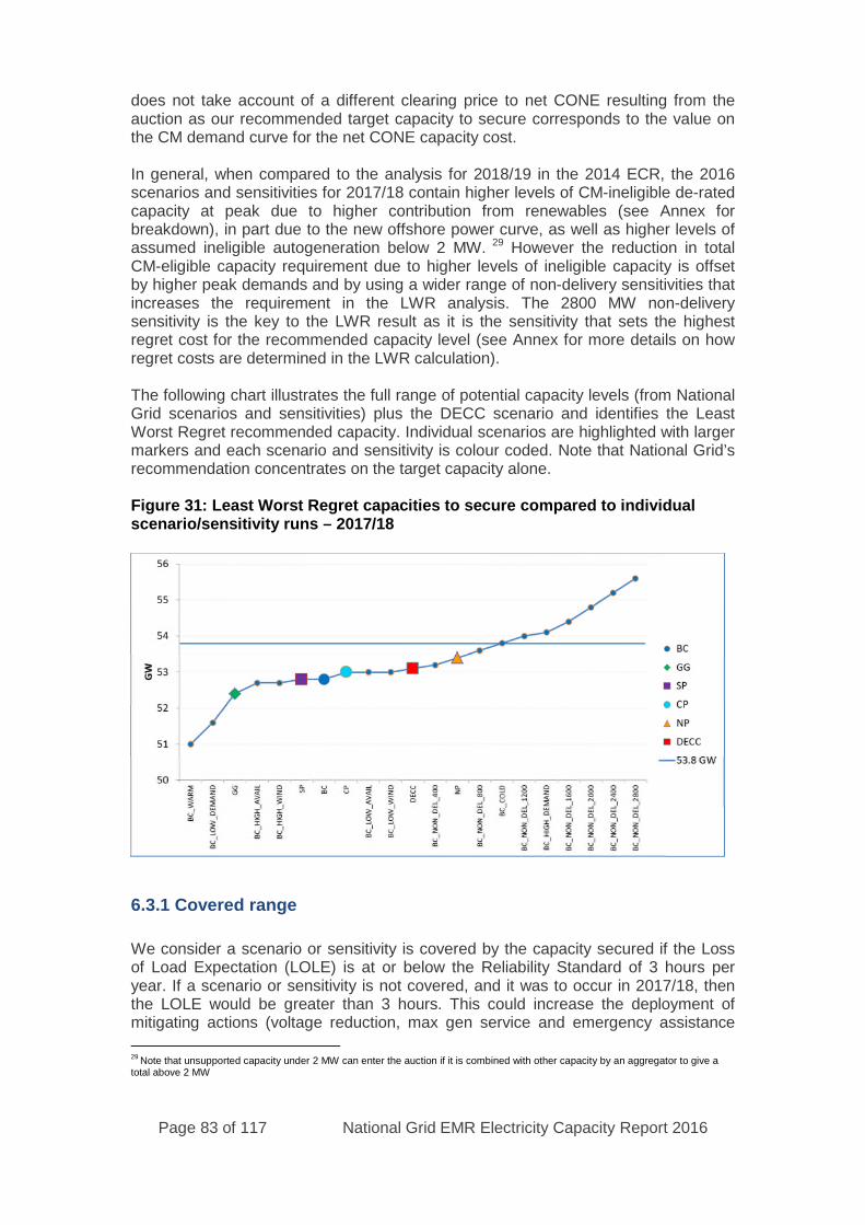
Page 83 of 117 National Grid EMR Electricity Capacity Report 2016
does not take account of a different clearing price to net CONE resulting from theauction as our recommended target capacity to secure corresponds to the value onthe CM demand curve for the net CONE capacity cost.
In general, when compared to the analysis for 2018/19 in the 2014 ECR, the 2016scenarios and sensitivities for 2017/18 contain higher levels of CM-ineligible de-ratedcapacity at peak due to higher contribution from renewables (see Annex forbreakdown), in part due to the new offshore power curve, as well as higher levels ofassumed ineligible autogeneration below 2 MW. 29 However the reduction in totalCM-eligible capacity requirement due to higher levels of ineligible capacity is offsetby higher peak demands and by using a wider range of non-delivery sensitivities thatincreases the requirement in the LWR analysis. The 2800 MW non-deliverysensitivity is the key to the LWR result as it is the sensitivity that sets the highestregret cost for the recommended capacity level (see Annex for more details on howregret costs are determined in the LWR calculation).
The following chart illustrates the full range of potential capacity levels (from NationalGrid scenarios and sensitivities) plus the DECC scenario and identifies the LeastWorst Regret recommended capacity. Individual scenarios are highlighted with largermarkers and each scenario and sensitivity is colour coded. Note that National Grid’srecommendation concentrates on the target capacity alone.
Figure 31: Least Worst Regret capacities to secure compared to individualscenario/sensitivity runs – 2017/18
6.3.1 Covered range
We consider a scenario or sensitivity is covered by the capacity secured if the Lossof Load Expectation (LOLE) is at or below the Reliability Standard of 3 hours peryear. If a scenario or sensitivity is not covered, and it was to occur in 2017/18, thenthe LOLE would be greater than 3 hours. This could increase the deployment ofmitigating actions (voltage reduction, max gen service and emergency assistance
29Note that unsupported capacity under 2 MW can enter the auction if it is combined with other capacity by an aggregator to give a
total above 2 MW
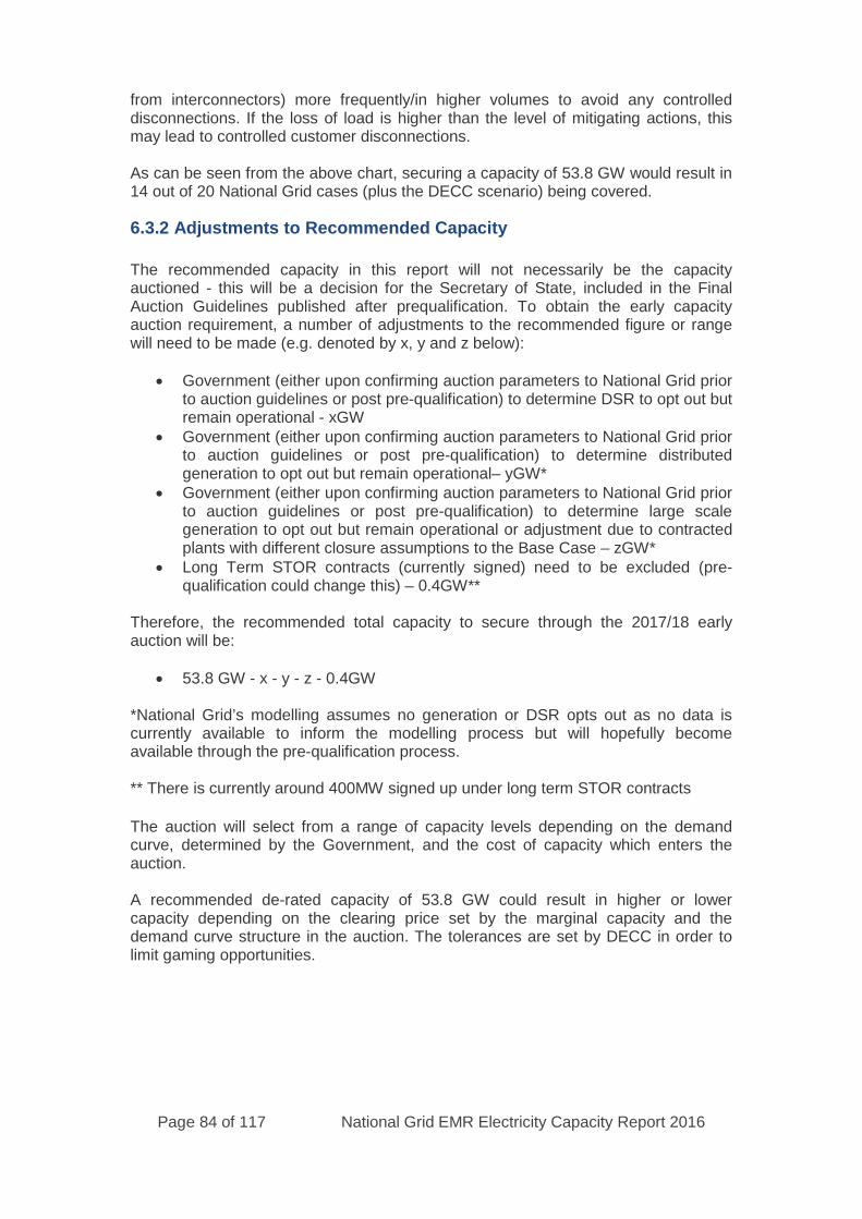
Page 84 of 117 National Grid EMR Electricity Capacity Report 2016
from interconnectors) more frequently/in higher volumes to avoid any controlleddisconnections. If the loss of load is higher than the level of mitigating actions, thismay lead to controlled customer disconnections.
As can be seen from the above chart, securing a capacity of 53.8 GW would result in14 out of 20 National Grid cases (plus the DECC scenario) being covered.
6.3.2 Adjustments to Recommended Capacity
The recommended capacity in this report will not necessarily be the capacityauctioned - this will be a decision for the Secretary of State, included in the FinalAuction Guidelines published after prequalification. To obtain the early capacityauction requirement, a number of adjustments to the recommended figure or rangewill need to be made (e.g. denoted by x, y and z below):
Government (either upon confirming auction parameters to National Grid priorto auction guidelines or post pre-qualification) to determine DSR to opt out butremain operational - xGW
Government (either upon confirming auction parameters to National Grid priorto auction guidelines or post pre-qualification) to determine distributedgeneration to opt out but remain operational– yGW*
Government (either upon confirming auction parameters to National Grid priorto auction guidelines or post pre-qualification) to determine large scalegeneration to opt out but remain operational or adjustment due to contractedplants with different closure assumptions to the Base Case – zGW*
Long Term STOR contracts (currently signed) need to be excluded (pre-qualification could change this) – 0.4GW**
Therefore, the recommended total capacity to secure through the 2017/18 earlyauction will be:
53.8 GW - x - y - z - 0.4GW
*National Grid’s modelling assumes no generation or DSR opts out as no data iscurrently available to inform the modelling process but will hopefully becomeavailable through the pre-qualification process.
** There is currently around 400MW signed up under long term STOR contracts
The auction will select from a range of capacity levels depending on the demandcurve, determined by the Government, and the cost of capacity which enters theauction.
A recommended de-rated capacity of 53.8 GW could result in higher or lowercapacity depending on the clearing price set by the marginal capacity and thedemand curve structure in the auction. The tolerances are set by DECC in order tolimit gaming opportunities.
Page 85 of 117 National Grid EMR Electricity Capacity Report 2016
7. Results and Indicative T-1Requirement for 2018/19 Auction
This chapter presents the results for 2018/19 only from the modelling of thescenarios and sensitivities relevant to 2018/19. We are not making arecommendation for 2018/19: these are provided for information only and have beenused to derive an indicative requirement for the 2018/19 T-1 auction Results andrecommendations for 2017/18 and 2020/21 can be found in chapters 5 and 6respectively. Further information on capacity requirements in years out to 2030/31can be found in section 3.11.
7.1 Sensitivities to model
The analysis assumes that the FES scenarios will cover uncertainty by incorporatingranges for annual and peak demand, DSR, interconnection and generation with thesensitivities covering uncertainty in single variables. In the modelling we haveassumed a net GB interconnector flow of 1900 MW in 2018/19 for the scenarios.Chapter 3 describes the scenarios and sensitivities modelled for the 2016 ECR. Theagreed sensitivities to model for 2018/19 cover non-delivery, weather, plantavailability, demand and interconnector peak flows:
Low Wind Output at times of cold weather (LOW WIND) High Wind Output at times of cold weather (HIGH WIND) Weather Cold Winter (COLD) Weather Warm Winter (WARM) High Plant Availabilities (HIGH AVAIL) Low Plant Availabilities (LOW AVAIL) High Demand (HIGH DEMAND) Low Demand (LOW DEMAND) Non Delivery (NON DEL): 9 sensitivities in 400 MW increments up to 3600
MW. 750 MW Continental interconnector imports (IC 750IMPORTS): 300 MW net
GB flow (including 450 MW exports to Ireland) 1500 MW Continental interconnector imports (IC 1500IMPORTS): 1300 MW
net GB flow (including 200 MW exports to Ireland) 2250 MW Continental interconnector imports (IC 2250IMPORTS): 2500 MW
net GB flow (including 250 MW imports from Ireland) 3000 MW Continental interconnector imports (IC 3000IMPORTS): 3500 MW
net GB flow (including 500 MW imports from Ireland)
7.2 Results
The following table shows the modelling results sorted in order of capacity to secureto meet the 3 hours LOLE Reliability Standard. It also shows the capacity outside ofthe CM, the total de-rated capacity and ACS peak demand.
The Base Case also assumes that some capacity contracted for 2018/19 in theprevious T-4 auction is not able to honour its awarded contracts. For example, the
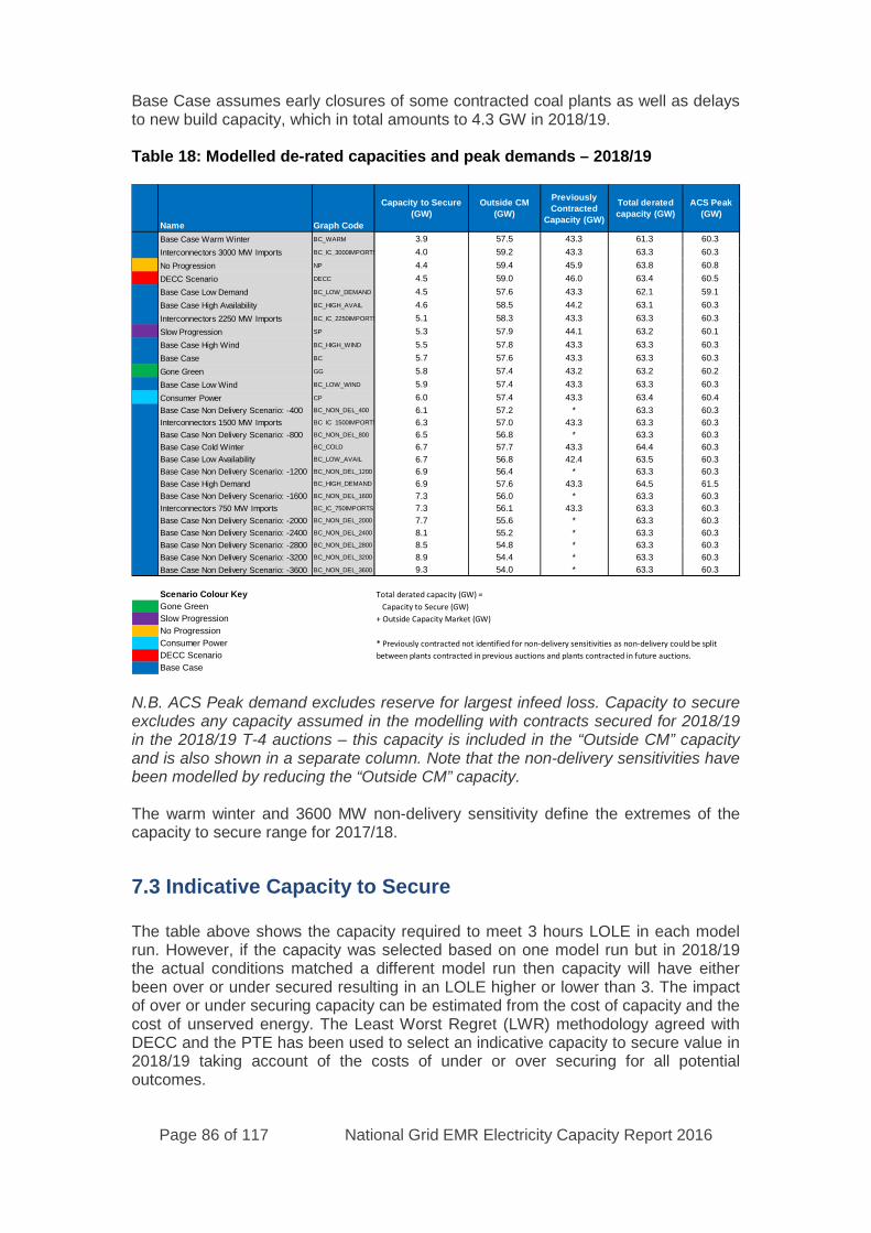
Page 86 of 117 National Grid EMR Electricity Capacity Report 2016
Base Case assumes early closures of some contracted coal plants as well as delaysto new build capacity, which in total amounts to 4.3 GW in 2018/19.
Table 18: Modelled de-rated capacities and peak demands – 2018/19
N.B. ACS Peak demand excludes reserve for largest infeed loss. Capacity to secureexcludes any capacity assumed in the modelling with contracts secured for 2018/19in the 2018/19 T-4 auctions – this capacity is included in the “Outside CM” capacityand is also shown in a separate column. Note that the non-delivery sensitivities havebeen modelled by reducing the “Outside CM” capacity.
The warm winter and 3600 MW non-delivery sensitivity define the extremes of thecapacity to secure range for 2017/18.
7.3 Indicative Capacity to Secure
The table above shows the capacity required to meet 3 hours LOLE in each modelrun. However, if the capacity was selected based on one model run but in 2018/19the actual conditions matched a different model run then capacity will have eitherbeen over or under secured resulting in an LOLE higher or lower than 3. The impactof over or under securing capacity can be estimated from the cost of capacity and thecost of unserved energy. The Least Worst Regret (LWR) methodology agreed withDECC and the PTE has been used to select an indicative capacity to secure value in2018/19 taking account of the costs of under or over securing for all potentialoutcomes.
Name Graph Code
Capacity to Secure
(GW)
Outside CM
(GW)
Previously
Contracted
Capacity (GW)
Total derated
capacity (GW)
ACS Peak
(GW)
Base Case Warm Winter BC_WARM 3.9 57.5 43.3 61.3 60.3
Interconnectors 3000 MW Imports BC_IC_3000IMPORTS 4.0 59.2 43.3 63.3 60.3
No Progression NP 4.4 59.4 45.9 63.8 60.8
DECC Scenario DECC 4.5 59.0 46.0 63.4 60.5
Base Case Low Demand BC_LOW_DEMAND 4.5 57.6 43.3 62.1 59.1
Base Case High Availability BC_HIGH_AVAIL 4.6 58.5 44.2 63.1 60.3
Interconnectors 2250 MW Imports BC_IC_2250IMPORTS 5.1 58.3 43.3 63.3 60.3
Slow Progression SP 5.3 57.9 44.1 63.2 60.1
Base Case High Wind BC_HIGH_WIND 5.5 57.8 43.3 63.3 60.3
Base Case BC 5.7 57.6 43.3 63.3 60.3
Gone Green GG 5.8 57.4 43.2 63.2 60.2
Base Case Low Wind BC_LOW_WIND 5.9 57.4 43.3 63.3 60.3
Consumer Power CP 6.0 57.4 43.3 63.4 60.4
Base Case Non Delivery Scenario: -400 BC_NON_DEL_400 6.1 57.2 * 63.3 60.3
Interconnectors 1500 MW Imports BC_IC_1500IMPORTS 6.3 57.0 43.3 63.3 60.3
Base Case Non Delivery Scenario: -800 BC_NON_DEL_800 6.5 56.8 * 63.3 60.3
Base Case Cold Winter BC_COLD 6.7 57.7 43.3 64.4 60.3
Base Case Low Availability BC_LOW_AVAIL 6.7 56.8 42.4 63.5 60.3
Base Case Non Delivery Scenario: -1200 BC_NON_DEL_1200 6.9 56.4 * 63.3 60.3
Base Case High Demand BC_HIGH_DEMAND 6.9 57.6 43.3 64.5 61.5
Base Case Non Delivery Scenario: -1600 BC_NON_DEL_1600 7.3 56.0 * 63.3 60.3
Interconnectors 750 MW Imports BC_IC_750IMPORTS 7.3 56.1 43.3 63.3 60.3
Base Case Non Delivery Scenario: -2000 BC_NON_DEL_2000 7.7 55.6 * 63.3 60.3
Base Case Non Delivery Scenario: -2400 BC_NON_DEL_2400 8.1 55.2 * 63.3 60.3
Base Case Non Delivery Scenario: -2800 BC_NON_DEL_2800 8.5 54.8 * 63.3 60.3
Base Case Non Delivery Scenario: -3200 BC_NON_DEL_3200 8.9 54.4 * 63.3 60.3
Base Case Non Delivery Scenario: -3600 BC_NON_DEL_3600 9.3 54.0 * 63.3 60.3
Scenario Colour Key Total derated capacity (GW) =
Gone Green Capacity to Secure (GW)
Slow Progression + Outside Capacity Market (GW)
No Progression
Consumer Power * Previously contracted not identified for non-delivery sensitivities as non-delivery could be split
DECC Scenario between plants contracted in previous auctions and plants contracted in future auctions.
Base Case
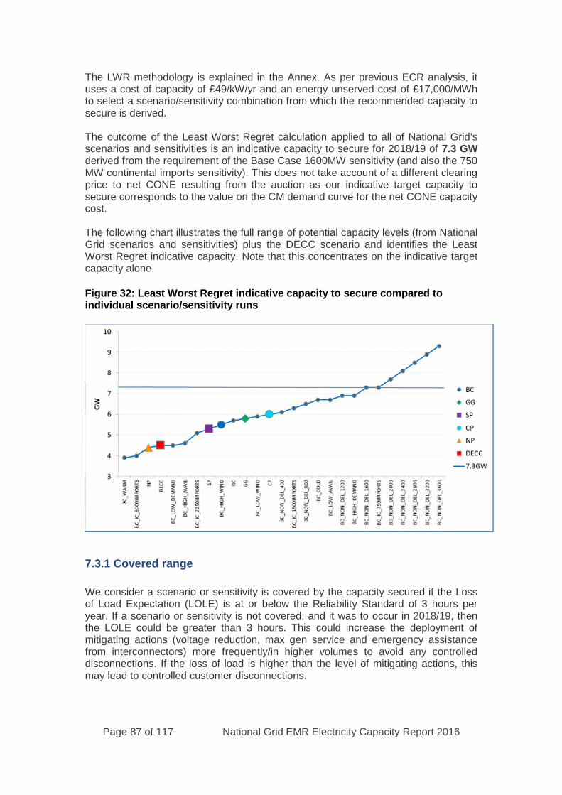
Page 87 of 117 National Grid EMR Electricity Capacity Report 2016
The LWR methodology is explained in the Annex. As per previous ECR analysis, ituses a cost of capacity of £49/kW/yr and an energy unserved cost of £17,000/MWhto select a scenario/sensitivity combination from which the recommended capacity tosecure is derived.
The outcome of the Least Worst Regret calculation applied to all of National Grid’sscenarios and sensitivities is an indicative capacity to secure for 2018/19 of 7.3 GWderived from the requirement of the Base Case 1600MW sensitivity (and also the 750MW continental imports sensitivity). This does not take account of a different clearingprice to net CONE resulting from the auction as our indicative target capacity tosecure corresponds to the value on the CM demand curve for the net CONE capacitycost.
The following chart illustrates the full range of potential capacity levels (from NationalGrid scenarios and sensitivities) plus the DECC scenario and identifies the LeastWorst Regret indicative capacity. Note that this concentrates on the indicative targetcapacity alone.
Figure 32: Least Worst Regret indicative capacity to secure compared toindividual scenario/sensitivity runs
7.3.1 Covered range
We consider a scenario or sensitivity is covered by the capacity secured if the Lossof Load Expectation (LOLE) is at or below the Reliability Standard of 3 hours peryear. If a scenario or sensitivity is not covered, and it was to occur in 2018/19, thenthe LOLE could be greater than 3 hours. This could increase the deployment ofmitigating actions (voltage reduction, max gen service and emergency assistancefrom interconnectors) more frequently/in higher volumes to avoid any controlleddisconnections. If the loss of load is higher than the level of mitigating actions, thismay lead to controlled customer disconnections.
Page 88 of 117 National Grid EMR Electricity Capacity Report 2016
As can be seen from the above chart, securing a capacity of 7.3 GW would result in21 out of 26 National Grid cases (plus the DECC scenario) being covered.
7.3.2 Adjustments to Indicative Capacity
The indicative capacity in this report (if it became the recommended capacity) wouldnot necessarily be the capacity auctioned - this will be a decision for the Secretary ofState, included in the Final Auction Guidelines published after prequalification. Toobtain the T-1 auction target, a number of adjustments to the indicative figure orrange may need to be made (e.g. denoted by x, y and z below) including a potentialadjustment to the previously contracted capacity assumed in the modelling (in z):
Government (either upon confirming auction parameters to National Grid priorto auction guidelines or post pre-qualification) to determine DSR to opt out butremain operational - xGW
Government (either upon confirming auction parameters to National Grid priorto auction guidelines or post pre-qualification) to determine distributedgeneration to opt out but remain operational– yGW*
Government (either upon confirming auction parameters to National Grid priorto auction guidelines or post pre-qualification) to determine large scalegeneration to opt out but remain operational or adjustment due to contractedplants with different closure assumptions to the Base Case – zGW*
Long Term STOR contracts (currently signed) need to be excluded (pre-qualification could change this) – 0.4GW**
Therefore, the indicative capacity to secure through the 2018/19 T-1 auction couldbe:
7.3 GW - x - y - z - 0.4GW
*National Grid’s modelling assumes no generation or DSR opts out as no data iscurrently available to inform the modelling process but will hopefully becomeavailable through the pre-qualification process. Furthermore, we expect DSR will bidinto the transitional auction.
** There is currently around 400MW signed up under long term STOR contracts
The auction will select from a range of capacity levels depending on the demandcurve, determined by the Government, and the cost of capacity which enters theauction.
An indicative de-rated capacity of 7.3 GW could result in a differing capacity volumebeing secured depending on the clearing price set by the marginal capacity and theshape of the demand curve. The tolerances are set by DECC in order to limit gamingopportunities.
7.3.3 Comparison with 2018/19 recommendation
In our 2014 Electricity Capacity Report, we recommended a capacity to secure for2018/19 of 53.3 GW of which the Secretary of State decided to hold back 2.5 GW forthe 2018/19 T-1 auction leaving a target capacity of 50.8 GW for the T-4 auction.Following pre-qualification, the 2018/19 T-4 auction target was reduced by 2.2 GW to48.6 GW to take account of 2.1 GW of transmission connected capacity that was

Page 89 of 117 National Grid EMR Electricity Capacity Report 2016
opted out but operational in 2018/19 and 0.1 GW of long-term STOR opted outcapacity. In the latest T-4 auction CM register for 2018/19, there is 49.2 GW of non-terminated awarded capacity, higher than the 48.6 GW target due to the low clearingprice.
In general, when compared to the analysis for 2018/19 in the 2014 ECR, the 2016scenarios and sensitivities for 2018/19 contain higher levels of CM-ineligible de-ratedcapacity at peak due to:
higher renewables contribution (see Annex for breakdown) in part due to thenew offshore power curve
higher levels of assumed opted-out or ineligible (below 2 MW)autogeneration30
1.9 GW higher assumed imports at peak in the Base Case over-securing in the 2018/19 T-4 auction.
However the reduction (compared to the 2014 ECR recommendation) in the T-1 CM-eligible capacity requirement due to higher levels of ineligible capacity is more thanoffset by:
a wider range of non-delivery sensitivities that increases the requirement inthe LWR analysis
assumed closures of contracted coal plants and delays to new build capacity,totalling 4.3 GW in 2018/19 in the Base Case.
the contracted capacity in the T-4 auction being greater than de-rated TEC “opted out but operational” plant closing higher peak demand in 2018/19 for the Base Case compared to the 2014
Slow Progression Low Availability sensitivity that set the 2014 ECRrecommendation
The Warm Winter sensitivity is key to the LWR result as it is the sensitivity that setsthe highest regret cost for the recommended capacity level (see Annex for moredetails on how regret costs are determined in the LWR calculation).
This indicative view highlights the risk of contracted coal plant defaulting throughclosures (up to 2.7 GW in the Base Case plus up to a further 3.6 GW in the mostextreme non-delivery sensitivity). However we note that by highlighting the risk in thisreport, some of these closures may be prevented which in turn would reduce thedemand curve target in the T-1 auction, which will be reassessed in the 2017 ECR.For example, if the 2.7 GW of coal closures assumed in the Base Case did not occur,the 7.3 GW indicative requirement would potentially drop by 2.7 GW to 4.6 GW.
The following waterfall chart shows how the original 2.5 GW requirement for the2018/19 T-1 auction (derived from the 2014 Slow Progression Low Availabilitysensitivity) has changed into an indicative requirement of 7.3 GW (derived from the2016 Base Case 1600 MW non-delivery sensitivity).
30Note that unsupported capacity under 2 MW can enter the auction if it is combined with other capacity by an aggregator to give a
total above 2 MW
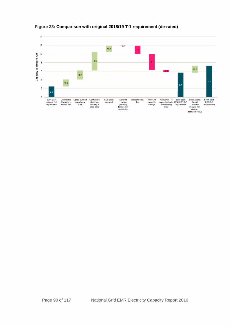
Page 90 of 117 National Grid EMR Electricity Capacity Report 2016
Figure 33: Comparison with original 2018/19 T-1 requirement (de-rated)
Page 91 of 117 National Grid EMR Electricity Capacity Report 2016
A. Annex
A.1 Future Energy Scenario Method
As part of our stakeholder engagement we received feedback to clearly demonstratehow we build our scenarios and in particular understand more about ourassumptions. We have created a new framework approach for 2016, detailing whatassumptions we have made in the four scenarios across the political, economic,social and technological themes. Environmental assumptions are integrated acrossthe four themes.
Scenario world
The first layer of our scenario framework is the scenario world. This contains thebuilding blocks and inputs which are consistent across all of the scenarios; thenumber of scenarios, the axes on which they are placed and the fixed rules regardingsecurity of supply. The two axes are, as last year, ‘Prosperity’ and ‘Green ambition’.The four scenario names are also the same as last year; Gone Green, SlowProgression, No Progression and Consumer Power. In 2015 there were three fixedrules across the four scenarios. The majority of stakeholders told us that the LevyControl Framework did not fit as a rule, as it is short term and can be changed. Assuch, for 2016 the Levy Control Framework is an assumption.
Electricity security of supply: In all scenarios, and across the whole study period,there will be sufficient electricity generation to meet the security of supply ReliabilityStandard. The government set a Reliability Standard for the GB market at a levelwhich balances the impact of failure to deliver sufficient energy with the cost of thecapacity required to provide that energy. This standard is three hours per year loss ofload expectation (LOLE). LOLE measures the risk across the whole winter ofdemand exceeding supply under normal operation. It does not mean that there willbe a loss of supply for three hours per year. It gives an indication of the amount oftime the System Operator will need to use balancing tools across the winter period.These tools include voltage reduction (reducing voltage to reduce demand),maximum generation (accessing capacity which is outside of the generator’s usualoperating range) and interconnector assistance (calling upon extra power flows fromthe continent). In most cases loss of load would be managed without significantimpact on end consumers. The electricity generation backgrounds used in all of theFES scenarios have been developed to ensure that this standard is always met.
Assumptions
The second layer of the scenario framework is the assumptions; these are thevariables which are flexed at high, medium or low in each scenario. They namespecific policies, technologies or behaviours. The assumptions are grouped intopolitical, economic, social and technological themes.
Model levers
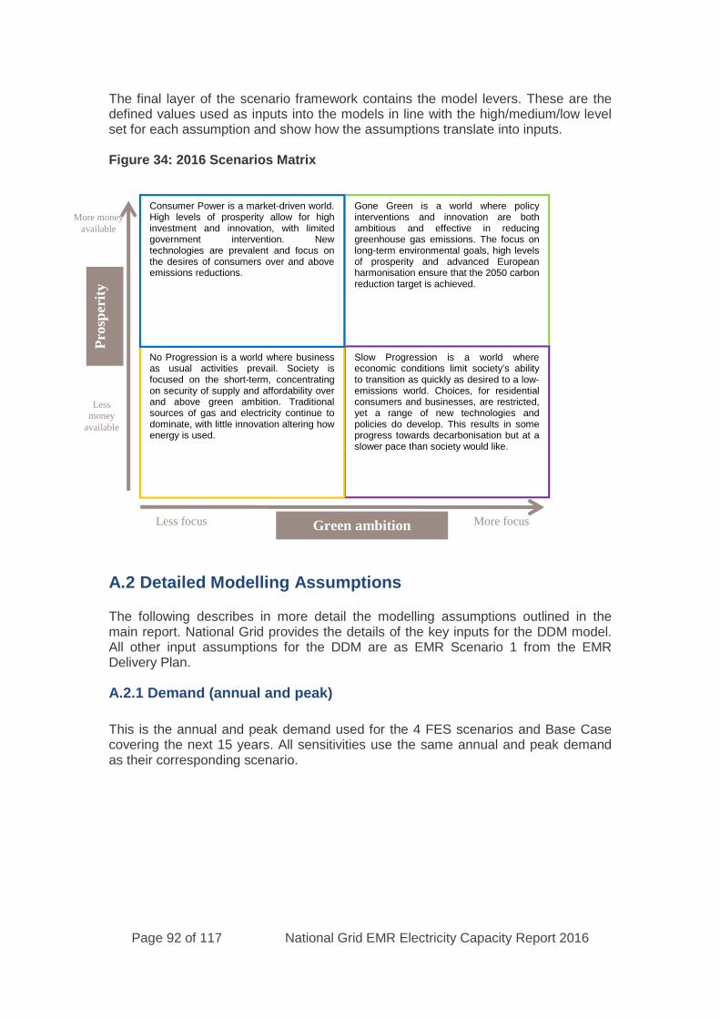
Page 92 of 117 National Grid EMR Electricity Capacity Report 2016
The final layer of the scenario framework contains the model levers. These are thedefined values used as inputs into the models in line with the high/medium/low levelset for each assumption and show how the assumptions translate into inputs.
Figure 34: 2016 Scenarios Matrix
Prosperity
A.2 Detailed Modelling Assumptions
The following describes in more detail the modelling assumptions outlined in themain report. National Grid provides the details of the key inputs for the DDM model.All other input assumptions for the DDM are as EMR Scenario 1 from the EMRDelivery Plan.
A.2.1 Demand (annual and peak)
This is the annual and peak demand used for the 4 FES scenarios and Base Casecovering the next 15 years. All sensitivities use the same annual and peak demandas their corresponding scenario.
Less focus More focusGreen ambition
Lessmoney
available
More moneyavailable
Pro
sper
ity
Gone Green is a world where policyinterventions and innovation are bothambitious and effective in reducinggreenhouse gas emissions. The focus onlong-term environmental goals, high levelsof prosperity and advanced Europeanharmonisation ensure that the 2050 carbonreduction target is achieved.
Slow Progression is a world whereeconomic conditions limit society’s abilityto transition as quickly as desired to a low-emissions world. Choices, for residentialconsumers and businesses, are restricted,yet a range of new technologies andpolicies do develop. This results in someprogress towards decarbonisation but at aslower pace than society would like.
No Progression is a world where businessas usual activities prevail. Society isfocused on the short-term, concentratingon security of supply and affordability overand above green ambition. Traditionalsources of gas and electricity continue todominate, with little innovation altering howenergy is used.
Consumer Power is a market-driven world.High levels of prosperity allow for highinvestment and innovation, with limitedgovernment intervention. Newtechnologies are prevalent and focus onthe desires of consumers over and aboveemissions reductions.
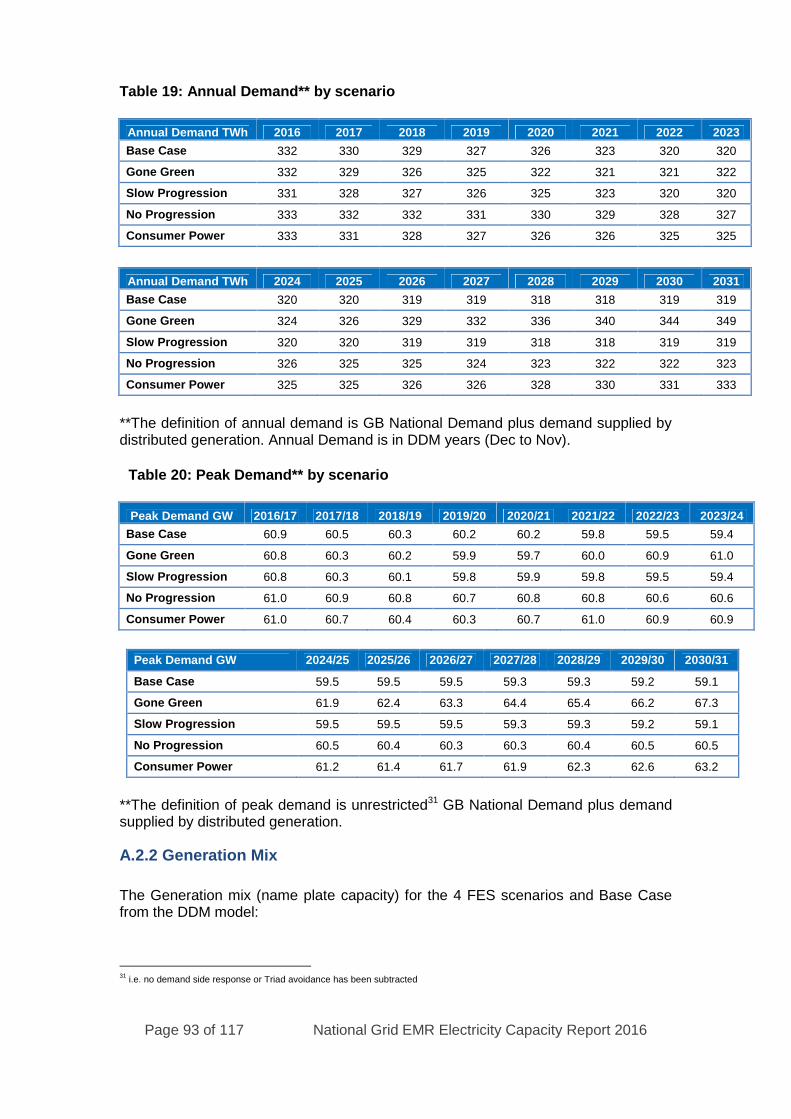
Page 93 of 117 National Grid EMR Electricity Capacity Report 2016
Table 19: Annual Demand** by scenario
Annual Demand TWh 2016 2017 2018 2019 2020 2021 2022 2023
Base Case 332 330 329 327 326 323 320 320
Gone Green 332 329 326 325 322 321 321 322
Slow Progression 331 328 327 326 325 323 320 320
No Progression 333 332 332 331 330 329 328 327
Consumer Power 333 331 328 327 326 326 325 325
Annual Demand TWh 2024 2025 2026 2027 2028 2029 2030 2031
Base Case 320 320 319 319 318 318 319 319
Gone Green 324 326 329 332 336 340 344 349
Slow Progression 320 320 319 319 318 318 319 319
No Progression 326 325 325 324 323 322 322 323
Consumer Power 325 325 326 326 328 330 331 333
**The definition of annual demand is GB National Demand plus demand supplied bydistributed generation. Annual Demand is in DDM years (Dec to Nov).
Table 20: Peak Demand** by scenario
Peak Demand GW 2016/17 2017/18 2018/19 2019/20 2020/21 2021/22 2022/23 2023/24
Base Case 60.9 60.5 60.3 60.2 60.2 59.8 59.5 59.4
Gone Green 60.8 60.3 60.2 59.9 59.7 60.0 60.9 61.0
Slow Progression 60.8 60.3 60.1 59.8 59.9 59.8 59.5 59.4
No Progression 61.0 60.9 60.8 60.7 60.8 60.8 60.6 60.6
Consumer Power 61.0 60.7 60.4 60.3 60.7 61.0 60.9 60.9
Peak Demand GW 2024/25 2025/26 2026/27 2027/28 2028/29 2029/30 2030/31
Base Case 59.5 59.5 59.5 59.3 59.3 59.2 59.1
Gone Green 61.9 62.4 63.3 64.4 65.4 66.2 67.3
Slow Progression 59.5 59.5 59.5 59.3 59.3 59.2 59.1
No Progression 60.5 60.4 60.3 60.3 60.4 60.5 60.5
Consumer Power 61.2 61.4 61.7 61.9 62.3 62.6 63.2
**The definition of peak demand is unrestricted31 GB National Demand plus demandsupplied by distributed generation.
A.2.2 Generation Mix
The Generation mix (name plate capacity) for the 4 FES scenarios and Base Casefrom the DDM model:
31i.e. no demand side response or Triad avoidance has been subtracted
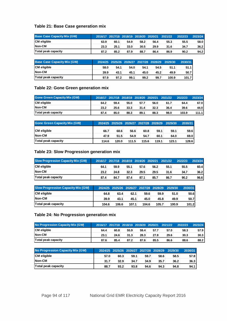
Page 94 of 117 National Grid EMR Electricity Capacity Report 2016
Table 21: Base Case generation mix
Table 22: Gone Green generation mix
Table 23: Slow Progression generation mix
Table 24: No Progression generation mix
Base Case Capacity Mix (GW) 2016/17 2017/18 2018/19 2019/20 2020/21 2021/22 2022/23 2023/24
CM eligible 63.9 60.1 54.9 58.2 56.4 55.3 55.5 58.0
Non-CM 23.3 25.1 33.0 30.5 29.9 31.6 34.7 36.2
Total peak capacity 87.2 85.2 87.9 88.7 86.4 86.9 90.2 94.2
Base Case Capacity Mix (GW) 2024/25 2025/26 2026/27 2027/28 2028/29 2029/30 2030/31
CM eligible 58.0 54.1 54.0 54.1 54.5 51.1 51.1
Non-CM 39.9 43.1 45.1 45.0 45.2 49.9 50.7
Total peak capacity 97.9 97.2 99.1 99.2 99.7 100.9 101.7
Gone Green Capacity Mix (GW) 2016/17 2017/18 2018/19 2019/20 2020/21 2021/22 2022/23 2023/24
CM eligible 64.2 59.4 55.0 57.7 56.0 61.7 64.4 67.0
Non-CM 23.2 25.6 33.3 31.4 32.3 36.4 39.6 44.0
Total peak capacity 87.4 85.0 88.3 89.1 88.3 98.0 103.9 111.1
Gone Green Capacity Mix (GW) 2024/25 2025/26 2026/27 2027/28 2028/29 2029/30 2030/31
CM eligible 66.7 68.6 56.6 60.8 59.1 59.1 59.6
Non-CM 47.9 51.5 54.9 54.7 60.1 64.0 69.0
Total peak capacity 114.6 120.0 111.5 115.6 119.1 123.1 128.6
Slow Progression Capacity Mix (GW) 2016/17 2017/18 2018/19 2019/20 2020/21 2021/22 2022/23 2023/24
CM eligible 64.1 59.9 55.1 57.6 56.2 55.1 55.5 60.4
Non-CM 23.2 24.8 32.3 29.5 29.5 31.6 34.7 36.2
Total peak capacity 87.4 84.7 87.4 87.1 85.7 86.7 90.2 96.6
Slow Progression Capacity Mix (GW) 2024/25 2025/26 2026/27 2027/28 2028/29 2029/30 2030/31
CM eligible 64.8 63.4 62.1 59.6 59.9 51.0 50.6
Non-CM 39.9 43.1 45.1 45.0 45.8 49.9 50.7
Total peak capacity 104.6 106.6 107.1 104.6 105.7 100.9 101.2
No Progression Capacity Mix (GW) 2016/17 2017/18 2018/19 2019/20 2020/21 2021/22 2022/23 2023/24
CM eligible 64.4 60.8 55.9 59.4 57.7 57.0 58.3 57.9
Non-CM 23.1 24.6 31.3 28.3 27.8 29.6 30.3 30.3
Total peak capacity 87.6 85.4 87.2 87.6 85.5 86.6 88.6 88.2
No Progression Capacity Mix (GW) 2024/25 2025/26 2026/27 2027/28 2028/29 2029/30 2030/31
CM eligible 57.0 60.3 59.1 59.7 58.6 58.5 57.8
Non-CM 31.7 32.9 34.7 34.9 35.7 36.2 36.3
Total peak capacity 88.7 93.2 93.8 94.6 94.3 94.8 94.1
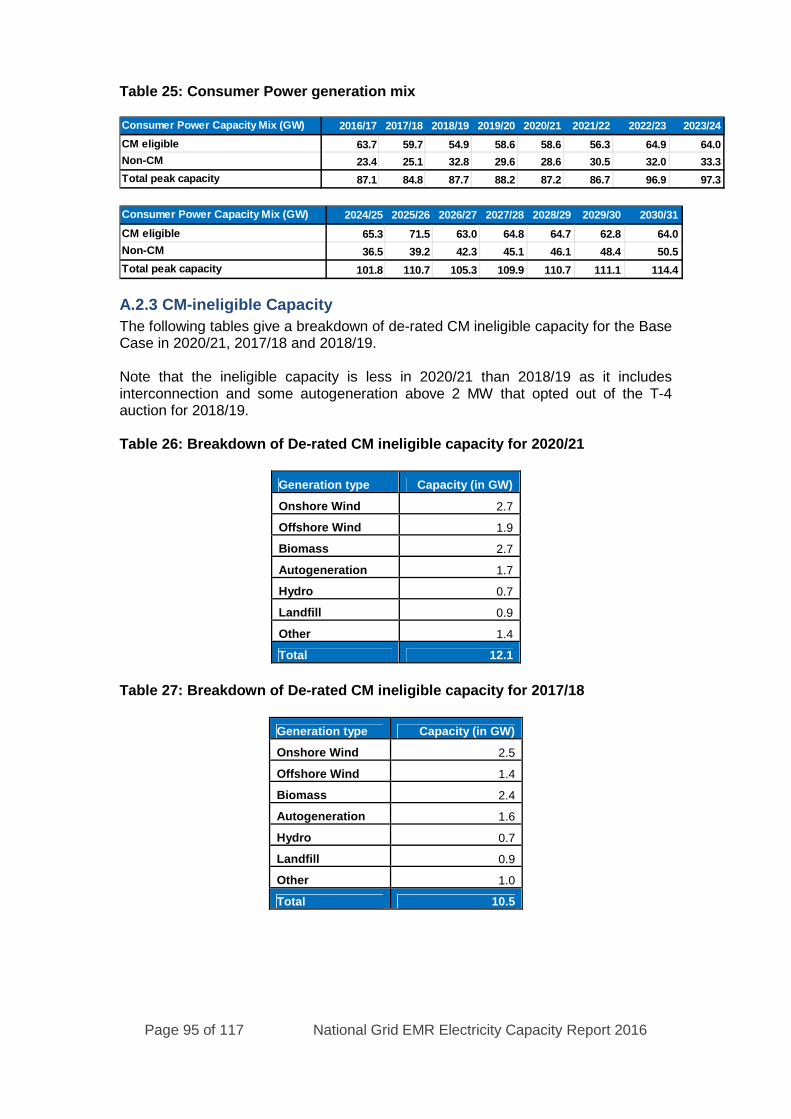
Page 95 of 117 National Grid EMR Electricity Capacity Report 2016
Table 25: Consumer Power generation mix
A.2.3 CM-ineligible Capacity
The following tables give a breakdown of de-rated CM ineligible capacity for the BaseCase in 2020/21, 2017/18 and 2018/19.
Note that the ineligible capacity is less in 2020/21 than 2018/19 as it includesinterconnection and some autogeneration above 2 MW that opted out of the T-4auction for 2018/19.
Table 26: Breakdown of De-rated CM ineligible capacity for 2020/21
Generation type Capacity (in GW)
Onshore Wind 2.7
Offshore Wind 1.9
Biomass 2.7
Autogeneration 1.7
Hydro 0.7
Landfill 0.9
Other 1.4
Total 12.1
Table 27: Breakdown of De-rated CM ineligible capacity for 2017/18
Generation type Capacity (in GW)
Onshore Wind 2.5
Offshore Wind 1.4
Biomass 2.4
Autogeneration 1.6
Hydro 0.7
Landfill 0.9
Other 1.0
Total 10.5
Consumer Power Capacity Mix (GW) 2016/17 2017/18 2018/19 2019/20 2020/21 2021/22 2022/23 2023/24
CM eligible 63.7 59.7 54.9 58.6 58.6 56.3 64.9 64.0
Non-CM 23.4 25.1 32.8 29.6 28.6 30.5 32.0 33.3
Total peak capacity 87.1 84.8 87.7 88.2 87.2 86.7 96.9 97.3
Consumer Power Capacity Mix (GW) 2024/25 2025/26 2026/27 2027/28 2028/29 2029/30 2030/31
CM eligible 65.3 71.5 63.0 64.8 64.7 62.8 64.0
Non-CM 36.5 39.2 42.3 45.1 46.1 48.4 50.5
Total peak capacity 101.8 110.7 105.3 109.9 110.7 111.1 114.4

Page 96 of 117 National Grid EMR Electricity Capacity Report 2016
Table 28: Breakdown of De-rated CM ineligible capacity for 2018/19
Generation type Capacity (in GW)
Onshore Wind 2.7
Offshore Wind 1.6
Biomass 2.7
Autogeneration 2.5
Interconnection 1.9
Hydro 0.7
Landfill 0.9
Other 1.2
Total 14.2
A.2.4 Station Availabilities
These are the station availabilities used for the 4 FES scenarios, base case, DECCScenario and the High and Low availability sensitivities (rounded to the nearest %).Note the two sensitivities cover the two most uncertain technologies of CCGT andNuclear.
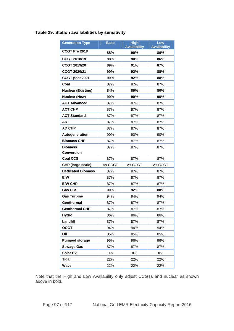
Page 97 of 117 National Grid EMR Electricity Capacity Report 2016
Table 29: Station availabilities by sensitivity
Generation Type Base HighAvailability
LowAvailability
CCGT Pre 2018 88% 90% 86%
CCGT 2018/19 88% 90% 86%
CCGT 2019/20 89% 91% 87%
CCGT 2020/21 90% 92% 88%
CCGT post 2021 90% 92% 88%
Coal 87% 87% 87%
Nuclear (Existing) 84% 89% 80%
Nuclear (New) 90% 90% 90%
ACT Advanced 87% 87% 87%
ACT CHP 87% 87% 87%
ACT Standard 87% 87% 87%
AD 87% 87% 87%
AD CHP 87% 87% 87%
Autogeneration 90% 90% 90%
Biomass CHP 87% 87% 87%
Biomass
Conversion
87% 87% 87%
Coal CCS 87% 87% 87%
CHP (large scale) As CCGT As CCGT As CCGT
Dedicated Biomass 87% 87% 87%
EfW 87% 87% 87%
EfW CHP 87% 87% 87%
Gas CCS 90% 92% 88%
Gas Turbine 94% 94% 94%
Geothermal 87% 87% 87%
Geothermal CHP 87% 87% 87%
Hydro 86% 86% 86%
Landfill 87% 87% 87%
OCGT 94% 94% 94%
Oil 85% 85% 85%
Pumped storage 96% 96% 96%
Sewage Gas 87% 87% 87%
Solar PV 0% 0% 0%
Tidal 22% 22% 22%
Wave 22% 22% 22%
Note that the High and Low Availability only adjust CCGTs and nuclear as shownabove in bold.
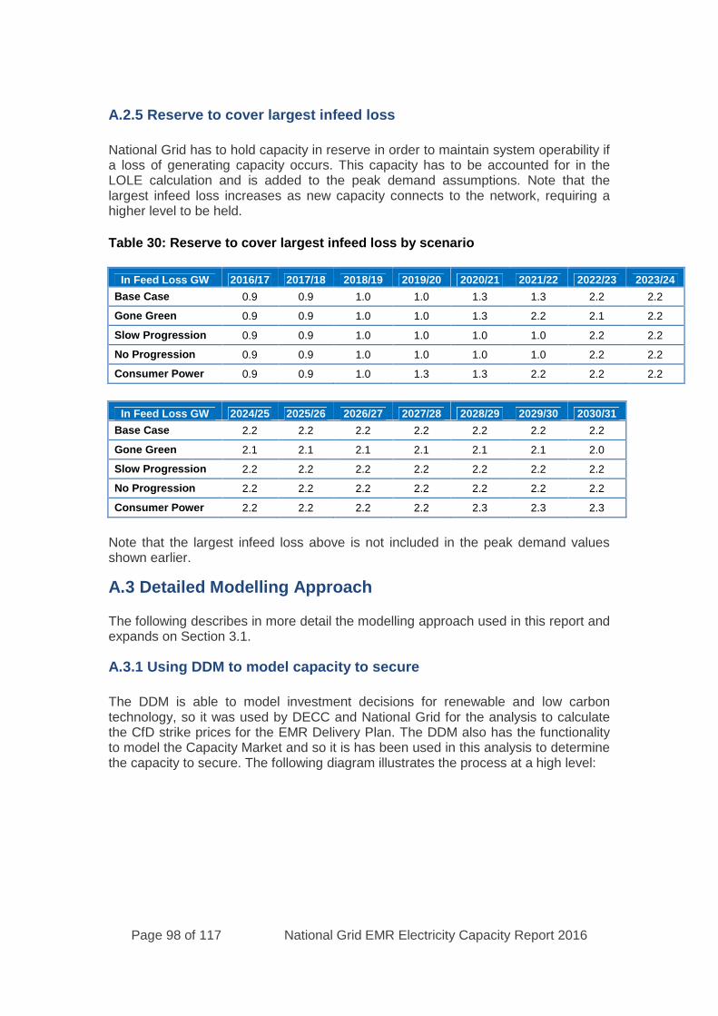
Page 98 of 117 National Grid EMR Electricity Capacity Report 2016
A.2.5 Reserve to cover largest infeed loss
National Grid has to hold capacity in reserve in order to maintain system operability ifa loss of generating capacity occurs. This capacity has to be accounted for in theLOLE calculation and is added to the peak demand assumptions. Note that thelargest infeed loss increases as new capacity connects to the network, requiring ahigher level to be held.
Table 30: Reserve to cover largest infeed loss by scenario
In Feed Loss GW 2016/17 2017/18 2018/19 2019/20 2020/21 2021/22 2022/23 2023/24
Base Case 0.9 0.9 1.0 1.0 1.3 1.3 2.2 2.2
Gone Green 0.9 0.9 1.0 1.0 1.3 2.2 2.1 2.2
Slow Progression 0.9 0.9 1.0 1.0 1.0 1.0 2.2 2.2
No Progression 0.9 0.9 1.0 1.0 1.0 1.0 2.2 2.2
Consumer Power 0.9 0.9 1.0 1.3 1.3 2.2 2.2 2.2
In Feed Loss GW 2024/25 2025/26 2026/27 2027/28 2028/29 2029/30 2030/31
Base Case 2.2 2.2 2.2 2.2 2.2 2.2 2.2
Gone Green 2.1 2.1 2.1 2.1 2.1 2.1 2.0
Slow Progression 2.2 2.2 2.2 2.2 2.2 2.2 2.2
No Progression 2.2 2.2 2.2 2.2 2.2 2.2 2.2
Consumer Power 2.2 2.2 2.2 2.2 2.3 2.3 2.3
Note that the largest infeed loss above is not included in the peak demand valuesshown earlier.
A.3 Detailed Modelling Approach
The following describes in more detail the modelling approach used in this report andexpands on Section 3.1.
A.3.1 Using DDM to model capacity to secure
The DDM is able to model investment decisions for renewable and low carbontechnology, so it was used by DECC and National Grid for the analysis to calculatethe CfD strike prices for the EMR Delivery Plan. The DDM also has the functionalityto model the Capacity Market and so it is has been used in this analysis to determinethe capacity to secure. The following diagram illustrates the process at a high level:

Page 99 of 117 National Grid EMR Electricity Capacity Report 2016
Figure 35: Capacity Market flow chart32
2020/21 Modelling Steps
The key steps in the modelling of the capacity to secure from 2020/21 are outlinedbelow:
1. The model first determines whether an auction should be run. For the2020/21 analysis, the first auction simulated is in 2016 for delivery in 2020/21.The model assumes that an auction is run in all subsequent years from 2016.
2. The generation capacity described in Chapter 3.6 generation (plus demandside response in 3.5) can be split into capacity that is eligible for the CapacityMarket and capacity that is not eligible for the Capacity Market. All of the non-eligible FES capacity is included in the modelling as this plant is determinedby the underlying scenario. The probabilistically modelled contribution ofinterconnection is included in the eligible capacity.
3. All of the non-eligible capacity has its de-rated capacity calculated, which mayinclude plants that have a Capacity Market agreement longer than a year ifthey are assumed to be operational in the scenario or sensitivity beingmodelled. This non-eligible capacity will be accounted for before any CapacityMarket auction is run. Note that the calculated de-rated capacity for acontracted plant may be different to the contracted capacity awarded in theauction.
32Chart supplied by Lane, Clark and Peacock LLP (LCP) http://www.lcp.uk.com/
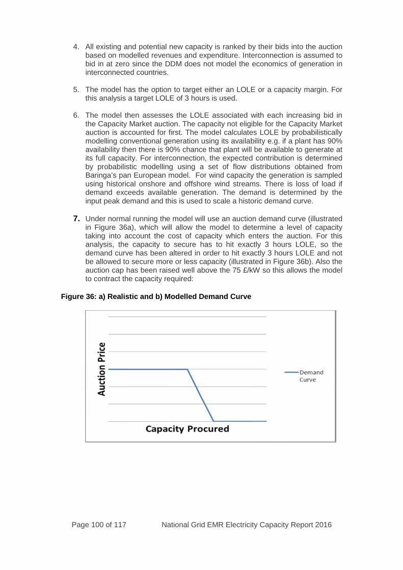
Page 100 of 117 National Grid EMR Electricity Capacity Report 2016
4. All existing and potential new capacity is ranked by their bids into the auctionbased on modelled revenues and expenditure. Interconnection is assumed tobid in at zero since the DDM does not model the economics of generation ininterconnected countries.
5. The model has the option to target either an LOLE or a capacity margin. Forthis analysis a target LOLE of 3 hours is used.
6. The model then assesses the LOLE associated with each increasing bid inthe Capacity Market auction. The capacity not eligible for the Capacity Marketauction is accounted for first. The model calculates LOLE by probabilisticallymodelling conventional generation using its availability e.g. if a plant has 90%availability then there is 90% chance that plant will be available to generate atits full capacity. For interconnection, the expected contribution is determinedby probabilistic modelling using a set of flow distributions obtained fromBaringa’s pan European model. For wind capacity the generation is sampledusing historical onshore and offshore wind streams. There is loss of load ifdemand exceeds available generation. The demand is determined by theinput peak demand and this is used to scale a historic demand curve.
7. Under normal running the model will use an auction demand curve (illustratedin Figure 36a), which will allow the model to determine a level of capacitytaking into account the cost of capacity which enters the auction. For thisanalysis, the capacity to secure has to hit exactly 3 hours LOLE, so thedemand curve has been altered in order to hit exactly 3 hours LOLE and notbe allowed to secure more or less capacity (illustrated in Figure 36b). Also theauction cap has been raised well above the 75 £/kW so this allows the modelto contract the capacity required:
Figure 36: a) Realistic and b) Modelled Demand Curve
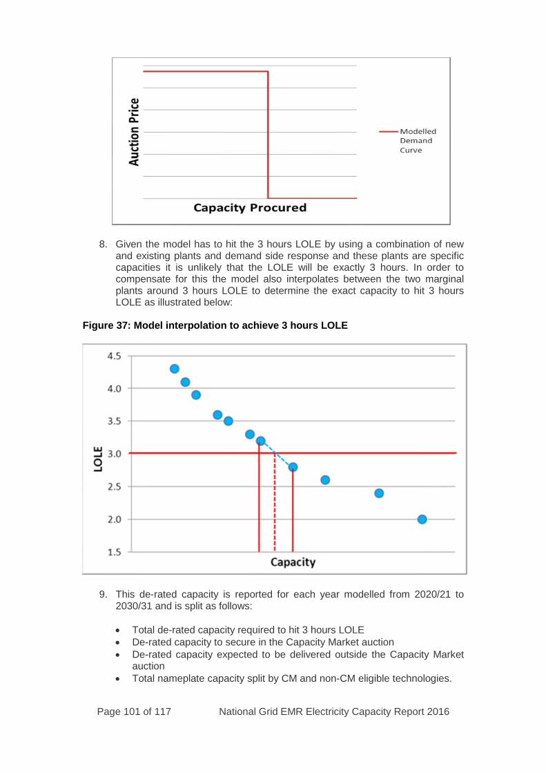
Page 101 of 117 National Grid EMR Electricity Capacity Report 2016
8. Given the model has to hit the 3 hours LOLE by using a combination of newand existing plants and demand side response and these plants are specificcapacities it is unlikely that the LOLE will be exactly 3 hours. In order tocompensate for this the model also interpolates between the two marginalplants around 3 hours LOLE to determine the exact capacity to hit 3 hoursLOLE as illustrated below:
Figure 37: Model interpolation to achieve 3 hours LOLE
9. This de-rated capacity is reported for each year modelled from 2020/21 to2030/31 and is split as follows:
Total de-rated capacity required to hit 3 hours LOLE De-rated capacity to secure in the Capacity Market auction De-rated capacity expected to be delivered outside the Capacity Market
auction Total nameplate capacity split by CM and non-CM eligible technologies.

Page 102 of 117 National Grid EMR Electricity Capacity Report 2016
2017/18 Modelling
For the 2017/18 analysis the modelling follows a similar process to the 2020/21analysis. The key differences in the modelling steps in A3.1.1 are highlighted below.
1. The first auction simulated is for delivery in 2017/18.
3. There is no previously contracted capacity for 2017/18.
9. Although the model assumes that auction is run in all subsequent years onlythe results for 2017/18 from this analysis have been used in this report.
2018/19 Modelling
For the 2018/19 analysis the modelling follows a similar process to the 2020/21analysis. The key differences in the modelling steps in A3.1.1 are highlighted below.
1. The first auction simulated is the T-1 auction for delivery in 2018/19.
3. The non-eligible capacity includes plants that have a Capacity Marketagreement for 2018/19 including (one year contracts as well as longercontracts if they are assumed to be operational in the scenario or sensitivitybeing modelled).
4. For interconnection in 2018/19, we have assumed a static peak flow that isconsistent with the de-rating factors used in the 2019/20 T-4 auction and arange of static flow sensitivities similar to those used in the ContingencyBalancing Reserve (CBR) analysis.
9. Although the model simulates auctions in later years only the results for2018/19 (and 2019/20) from this analysis have been used in this report.
A.3.2 Treatment of Generation Technologies
The DDM models a range of generation technology types. For this analysis they arethe same categories which were modelled in the EMR Delivery Plan. Most of thesetechnologies are assumed to either be eligible for the Capacity Market or not. Hydrocapacity is split between both categories.
For any technology receiving support, plants are eligible to participate in the CapacityMarket when this support has finished. Any unsupported generation capacity that isunder a total capacity of 2 MW is not eligible for the Capacity Market unless it iscombined with other capacity by an aggregator to give a total above 2 MW. Theunsupported generation capacity that is under 2 MW has been estimated by NationalGrid to range from 1.6 GW to 2.0 GW in the period to 2020/21 depending on the FESscenario and year.
The following table lists generation technologies modelled and whether they areassumed to be Capacity Market eligible or not (before support finishes).
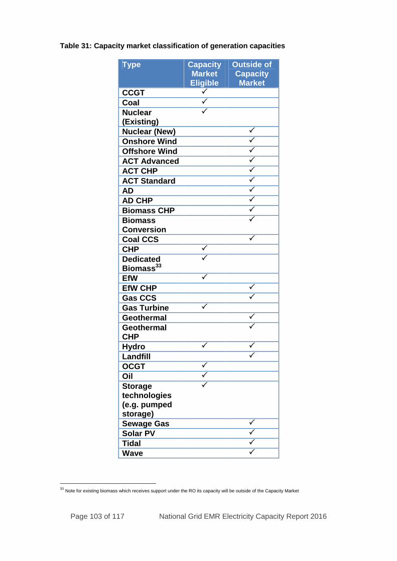
Page 103 of 117 National Grid EMR Electricity Capacity Report 2016
Table 31: Capacity market classification of generation capacities
Type CapacityMarketEligible
Outside ofCapacityMarket
CCGT
Coal
Nuclear(Existing)
Nuclear (New)
Onshore Wind
Offshore Wind
ACT Advanced
ACT CHP
ACT Standard
AD
AD CHP
Biomass CHP
BiomassConversion
Coal CCS
CHP
DedicatedBiomass33
EfW
EfW CHP
Gas CCS
Gas Turbine
Geothermal
GeothermalCHP
Hydro
Landfill
OCGT
Oil
Storagetechnologies(e.g. pumpedstorage)
Sewage Gas
Solar PV
Tidal
Wave
33Note for existing biomass which receives support under the RO its capacity will be outside of the Capacity Market
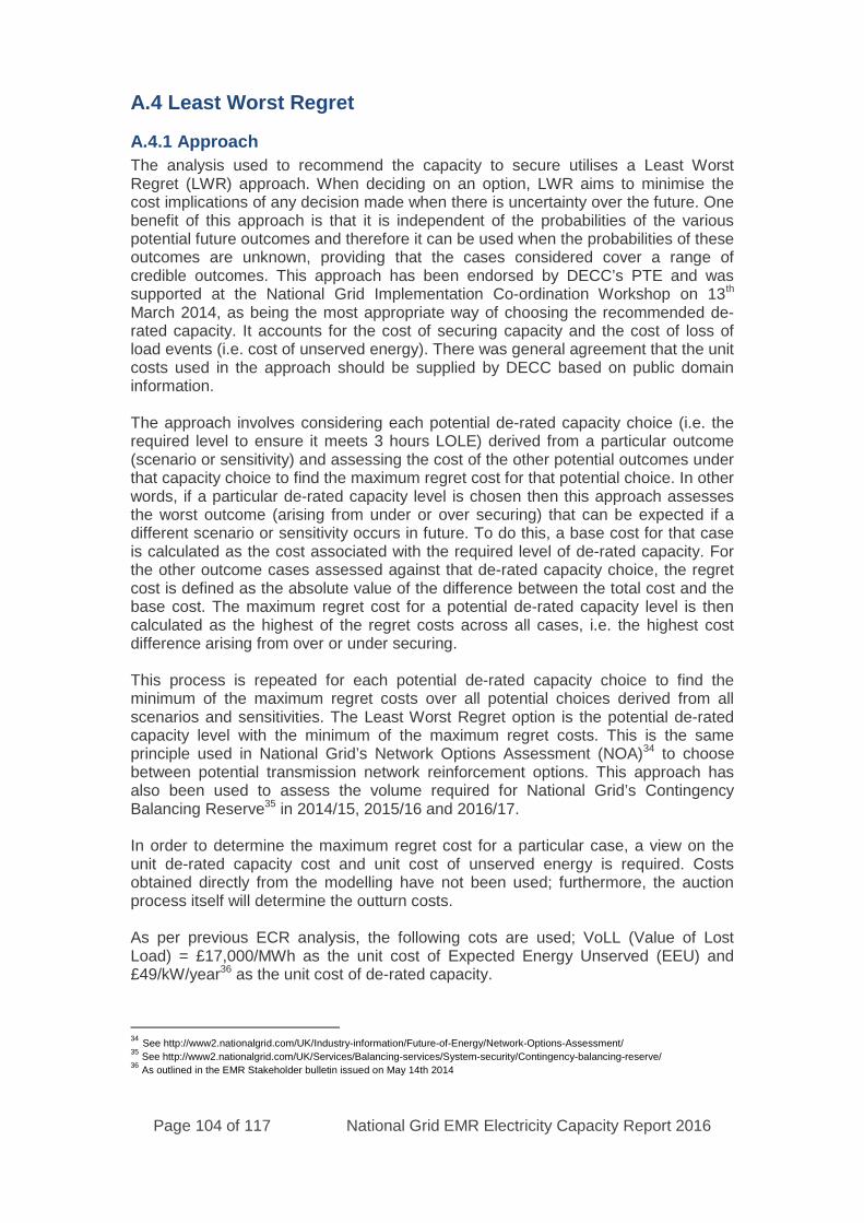
Page 104 of 117 National Grid EMR Electricity Capacity Report 2016
A.4 Least Worst Regret
A.4.1 Approach
The analysis used to recommend the capacity to secure utilises a Least WorstRegret (LWR) approach. When deciding on an option, LWR aims to minimise thecost implications of any decision made when there is uncertainty over the future. Onebenefit of this approach is that it is independent of the probabilities of the variouspotential future outcomes and therefore it can be used when the probabilities of theseoutcomes are unknown, providing that the cases considered cover a range ofcredible outcomes. This approach has been endorsed by DECC’s PTE and wassupported at the National Grid Implementation Co-ordination Workshop on 13th
March 2014, as being the most appropriate way of choosing the recommended de-rated capacity. It accounts for the cost of securing capacity and the cost of loss ofload events (i.e. cost of unserved energy). There was general agreement that the unitcosts used in the approach should be supplied by DECC based on public domaininformation.
The approach involves considering each potential de-rated capacity choice (i.e. therequired level to ensure it meets 3 hours LOLE) derived from a particular outcome(scenario or sensitivity) and assessing the cost of the other potential outcomes underthat capacity choice to find the maximum regret cost for that potential choice. In otherwords, if a particular de-rated capacity level is chosen then this approach assessesthe worst outcome (arising from under or over securing) that can be expected if adifferent scenario or sensitivity occurs in future. To do this, a base cost for that caseis calculated as the cost associated with the required level of de-rated capacity. Forthe other outcome cases assessed against that de-rated capacity choice, the regretcost is defined as the absolute value of the difference between the total cost and thebase cost. The maximum regret cost for a potential de-rated capacity level is thencalculated as the highest of the regret costs across all cases, i.e. the highest costdifference arising from over or under securing.
This process is repeated for each potential de-rated capacity choice to find theminimum of the maximum regret costs over all potential choices derived from allscenarios and sensitivities. The Least Worst Regret option is the potential de-ratedcapacity level with the minimum of the maximum regret costs. This is the sameprinciple used in National Grid’s Network Options Assessment (NOA)34 to choosebetween potential transmission network reinforcement options. This approach hasalso been used to assess the volume required for National Grid’s ContingencyBalancing Reserve35 in 2014/15, 2015/16 and 2016/17.
In order to determine the maximum regret cost for a particular case, a view on theunit de-rated capacity cost and unit cost of unserved energy is required. Costsobtained directly from the modelling have not been used; furthermore, the auctionprocess itself will determine the outturn costs.
As per previous ECR analysis, the following cots are used; VoLL (Value of LostLoad) = £17,000/MWh as the unit cost of Expected Energy Unserved (EEU) and£49/kW/year36 as the unit cost of de-rated capacity.
34See http://www2.nationalgrid.com/UK/Industry-information/Future-of-Energy/Network-Options-Assessment/
35See http://www2.nationalgrid.com/UK/Services/Balancing-services/System-security/Contingency-balancing-reserve/
36As outlined in the EMR Stakeholder bulletin issued on May 14th 2014
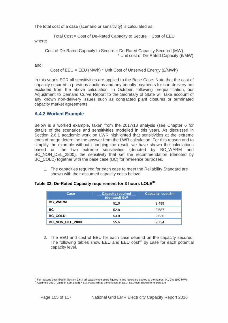
Page 105 of 117 National Grid EMR Electricity Capacity Report 2016
The total cost of a case (scenario or sensitivity) is calculated as:
Total Cost = Cost of De-Rated Capacity to Secure + Cost of EEUwhere:
Cost of De-Rated Capacity to Secure = De-Rated Capacity Secured (MW)* Unit cost of De-Rated Capacity (£/MW)
and:Cost of EEU = EEU (MWh) * Unit Cost of Unserved Energy (£/MWh)
In this year’s ECR all sensitivities are applied to the Base Case. Note that the cost ofcapacity secured in previous auctions and any penalty payments for non-delivery areexcluded from the above calculation. In October, following prequalification, ourAdjustment to Demand Curve Report to the Secretary of State will take account ofany known non-delivery issues such as contracted plant closures or terminatedcapacity market agreements.
A.4.2 Worked Example
Below is a worked example, taken from the 2017/18 analysis (see Chapter 6 fordetails of the scenarios and sensitivities modelled in this year). As discussed inSection 2.6.1 academic work on LWR highlighted that sensitivities at the extremeends of range determine the answer from the LWR calculation. For this reason and tosimplify the example without changing the result, we have shown the calculationsbased on the two extreme sensitivities (denoted by BC_WARM andBC_NON_DEL_2800), the sensitivity that set the recommendation (denoted byBC_COLD) together with the base case (BC) for reference purposes.
1. The capacities required for each case to meet the Reliability Standard areshown with their assumed capacity costs below:
Table 32: De-Rated Capacity requirement for 3 hours LOLE37
Case Capacity required(de-rated) GW
Capacity cost £m
BC_WARM 51.0 2,499
BC 52.8 2,587
BC_COLD 53.8 2,636
BC_NON_DEL_2800 55.6 2,724
2. The EEU and cost of EEU for each case depend on the capacity secured.The following tables show EEU and EEU cost38 by case for each potentialcapacity level.
37For reasons described in Section 2.6.3, all capacity to secure figures in this report are quoted to the nearest 0.1 GW (100 MW).
38Assumes VoLL (Value of Lost Load) = £17,000/MWh as the unit cost of EEU. EEU cost shown to nearest £m
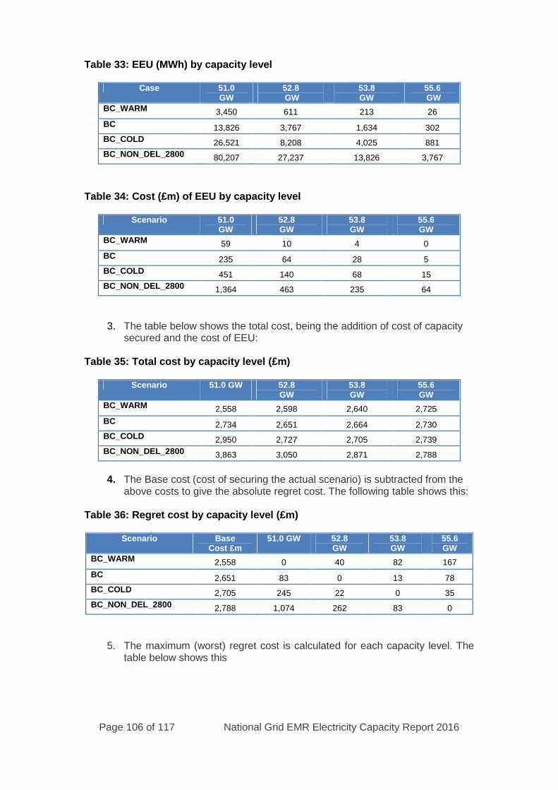
Page 106 of 117 National Grid EMR Electricity Capacity Report 2016
Table 33: EEU (MWh) by capacity level
Case 51.0GW
52.8GW
53.8GW
55.6GW
BC_WARM 3,450 611 213 26
BC 13,826 3,767 1,634 302
BC_COLD 26,521 8,208 4,025 881
BC_NON_DEL_2800 80,207 27,237 13,826 3,767
Table 34: Cost (£m) of EEU by capacity level
Scenario 51.0GW
52.8GW
53.8GW
55.6GW
BC_WARM 59 10 4 0
BC 235 64 28 5
BC_COLD 451 140 68 15
BC_NON_DEL_2800 1,364 463 235 64
3. The table below shows the total cost, being the addition of cost of capacitysecured and the cost of EEU:
Table 35: Total cost by capacity level (£m)
Scenario 51.0 GW 52.8GW
53.8GW
55.6GW
BC_WARM 2,558 2,598 2,640 2,725
BC 2,734 2,651 2,664 2,730
BC_COLD 2,950 2,727 2,705 2,739
BC_NON_DEL_2800 3,863 3,050 2,871 2,788
4. The Base cost (cost of securing the actual scenario) is subtracted from theabove costs to give the absolute regret cost. The following table shows this:
Table 36: Regret cost by capacity level (£m)
Scenario BaseCost £m
51.0 GW 52.8GW
53.8GW
55.6GW
BC_WARM 2,558 0 40 82 167
BC 2,651 83 0 13 78
BC_COLD 2,705 245 22 0 35
BC_NON_DEL_2800 2,788 1,074 262 83 0
5. The maximum (worst) regret cost is calculated for each capacity level. Thetable below shows this
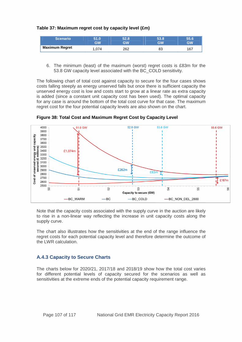
Page 107 of 117 National Grid EMR Electricity Capacity Report 2016
Table 37: Maximum regret cost by capacity level (£m)
Scenario 51.0GW
52.8GW
53.8GW
55.6GW
Maximum Regret 1,074 262 83 167
6. The minimum (least) of the maximum (worst) regret costs is £83m for the53.8 GW capacity level associated with the BC_COLD sensitivity.
The following chart of total cost against capacity to secure for the four cases showscosts falling steeply as energy unserved falls but once there is sufficient capacity theunserved energy cost is low and costs start to grow at a linear rate as extra capacityis added (since a constant unit capacity cost has been used). The optimal capacityfor any case is around the bottom of the total cost curve for that case. The maximumregret cost for the four potential capacity levels are also shown on the chart.
Figure 38: Total Cost and Maximum Regret Cost by Capacity Level
Note that the capacity costs associated with the supply curve in the auction are likelyto rise in a non-linear way reflecting the increase in unit capacity costs along thesupply curve.
The chart also illustrates how the sensitivities at the end of the range influence theregret costs for each potential capacity level and therefore determine the outcome ofthe LWR calculation.
A.4.3 Capacity to Secure Charts
The charts below for 2020/21, 2017/18 and 2018/19 show how the total cost variesfor different potential levels of capacity secured for the scenarios as well assensitivities at the extreme ends of the potential capacity requirement range.

Page 108 of 117 National Grid EMR Electricity Capacity Report 2016
Figure 39: Cost v Potential Capacity to Secure Levels 2020/21
Figure 40: Cost v Potential Capacity to Secure Levels 2017/18
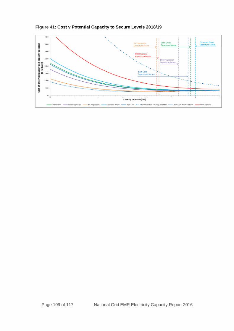
Page 109 of 117 National Grid EMR Electricity Capacity Report 2016
Figure 41: Cost v Potential Capacity to Secure Levels 2018/19
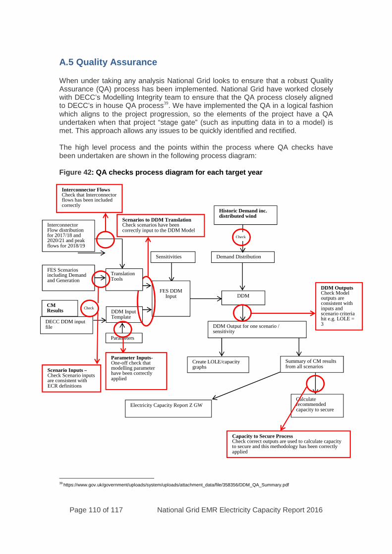
Page 110 of 117 National Grid EMR Electricity Capacity Report 2016
A.5 Quality Assurance
When under taking any analysis National Grid looks to ensure that a robust QualityAssurance (QA) process has been implemented. National Grid have worked closelywith DECC’s Modelling Integrity team to ensure that the QA process closely alignedto DECC’s in house QA process39. We have implemented the QA in a logical fashionwhich aligns to the project progression, so the elements of the project have a QAundertaken when that project “stage gate” (such as inputting data in to a model) ismet. This approach allows any issues to be quickly identified and rectified.
The high level process and the points within the process where QA checks havebeen undertaken are shown in the following process diagram:
Figure 42: QA checks process diagram for each target year
39https://www.gov.uk/government/uploads/system/uploads/attachment_data/file/358356/DDM_QA_Summary.pdf
Sensitivities
DDM InputTemplate
Parameters
DECC DDM inputfile
FES DDMInput
Scenario Inputs –Check Scenario inputsare consistent withECR definitions
Parameter Inputs-One-off check thatmodelling parameterhave been correctlyapplied
Create LOLE/capacitygraphs
Summary of CM resultsfrom all scenarios
Electricity Capacity Report Z GWCalculaterecommendedcapacity to secure
Capacity to Secure ProcessCheck correct outputs are used to calculate capacityto secure and this methodology has been correctlyapplied
DDM Output for one scenario /sensitivity
DDM
DDM OutputsCheck Modeloutputs areconsistent withinputs andscenario criteriahit e.g. LOLE =3
InterconnectorFlow distributionfor 2017/18 and2020/21 and peakflows for 2018/19
FES Scenariosincluding Demandand Generation
TranslationTools
Scenarios to DDM TranslationCheck scenarios have beencorrectly input to the DDM Model
Interconnector FlowsCheck that Interconnectorflows has been includedcorrectly
CMResults
Check
Historic Demand inc.distributed wind
Demand Distribution
Check

Page 111 of 117 National Grid EMR Electricity Capacity Report 2016
The QA checks above (bordered in red) are centred on the points in the processwhere data is transferred from one model, or system, to another along with the modeloutputs. The QA is undertaken in this way as it is more straight-forward to followwhich QA step is being applied at which step in the process. These steps are:
1. Interconnector flows – Check the interconnector flowassumption/distribution
2. Scenario inputs – Check the model input assumptions
3. Parameter Inputs / CM Results/ Historic Demand Including DistributedWind – Check the model setup assumptions
4. Scenarios to DDM Translation – Check the input from the FES processinto the DDM model
5. DDM Outputs - Check model outputs are consistent with inputs andscenario criteria
6. Capacity to Secure Process – Check the inputs and outputs used todetermine a range and recommended capacity to secure
Below is detailed QA process for each of these steps.
Interconnector flows
Interconnector flows assumption/distribution have been discussed with DECC, PTEand Ofgem at various bilateral meetings. We have also consulted the results with theindustry at various stakeholder events. For each scenarios, the modelledinterconnector flows and results are checked throughout the QA checklist process.
Scenario Inputs
The FES process is driven by extensive stakeholder engagement40, workshops andbilateral meetings; this engagement leads to the creation of the scenarios. Theconstituent parts of the scenarios, for example electricity demand, are subject tointernal challenge and review to ensure that they consistent and robust. Sign off isthen required at senior manager level and formal sign off is then required from theSO Executive Committee. The assumption and outputs will be published in theannual FES document on July 5th 2016.
For the purposes of the ECR process a check is undertaken that the inputs areconsistent with the requirements of the ECR process.
Parameter Inputs / CM Results/ Historic Demand Including DistributedWind
The parameters are set to ensure that the model runs as is required for the ECRprocess. These parameters are checked and documented by two analysts to ensurethat they are correct and then a final template is created (with a backup) which all
40http://www2.nationalgrid.com/UK/Industry-information/Future-of-Energy/FES/Engagement/
Page 112 of 117 National Grid EMR Electricity Capacity Report 2016
runs are then based on. This step also includes checking of the inputs like historicdemand, demand met by distributed wind and CM Results are correctly included inthe model.
Scenarios to DDM Translation
The tool for translating the FES scenarios into DDM has been documented andavailable for scrutiny by DECC and the PTE. The tool includes checks that thecorrect information has been inputted to the model.
DDM Outputs
Each run of the analysis, including inputs and outputs, has been checked anddocumented internally by an analyst not involved in the ECR modelling, but familiarwith the DDM and the ECR project. These documents and the associated files havebeen shared with DECC to allow it to perform its own QA process.
QA Check List Process
Each run of the analysis, including inputs and outputs, is checked and documentedinternally by an analyst through a QA Check List process.
Capacity to Secure Process
Once all the runs have been completed the key results are used to determine therecommended capacity to secure using Least Worst Regret (LWR) tool. This processhas been checked and documented internally by an analyst not involved in the ECRmodelling, but familiar with the DDM and ECR project. Again, these files have beenshared with DECC to allow it to perform its own QA process.
DDM model
In addition to checks described in above figure, DDM model has been reviewed andhad QA performed a number of times including:
A peer review by Prof. Newbery and Prof. Ralph A review of the code by PwC Internal reviews by DECC
Details of these can be found in the 2013 EMR Delivery Plan document. These implythat a further QA of the DDM is not required as part of the ECR QA process.However, to ensure that the DDM is the correct model to use, and that it is beingused correctly, the PTE have been specifically asked to QA the use of DDM for ECR.In previous years, the owners of DDM, consultants Lane Clarke Peacock (LCP41),were asked to ensure that National Grid was both using the model, and interpretingthe outputs, correctly. This involved a bilateral meeting between National Grid andLCP to discuss in detail the modelling being undertaken. This highlighted some minorissues which have been resolved. LCP produced a report of their QA process. Thereport concludes that National Grid is using the model correctly and correctlyinterpreting the output results.
41http://www.lcp.uk.com/

Page 113 of 117 National Grid EMR Electricity Capacity Report 2016
Process Overview and Governance
The process will be overseen by the PTE and they will review and report on theoverall process. Internally the process has governance under Director UK SystemOperator with final sign off by the Chief Executive.
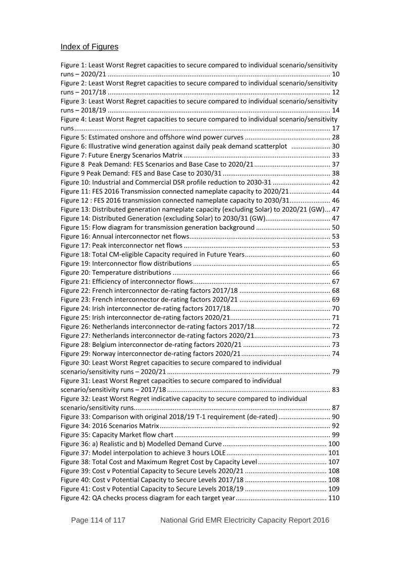
Page 114 of 117 National Grid EMR Electricity Capacity Report 2016
Index of Figures
Figure 1: Least Worst Regret capacities to secure compared to individual scenario/sensitivityruns – 2020/21 ........................................................................................................................ 10Figure 2: Least Worst Regret capacities to secure compared to individual scenario/sensitivityruns – 2017/18 ........................................................................................................................ 12Figure 3: Least Worst Regret capacities to secure compared to individual scenario/sensitivityruns – 2018/19 ........................................................................................................................ 14Figure 4: Least Worst Regret capacities to secure compared to individual scenario/sensitivityruns.......................................................................................................................................... 17Figure 5: Estimated onshore and offshore wind power curves .............................................. 28Figure 6: Illustrative wind generation against daily peak demand scatterplot ..................... 30Figure 7: Future Energy Scenarios Matrix ............................................................................... 33Figure 8 Peak Demand: FES Scenarios and Base Case to 2020/21......................................... 37Figure 9 Peak Demand: FES and Base Case to 2030/31 .......................................................... 38Figure 10: Industrial and Commercial DSR profile reduction to 2030-31 ............................... 42Figure 11: FES 2016 Transmission connected nameplate capacity to 2020/21...................... 44Figure 12 : FES 2016 transmission connected nameplate capacity to 2030/31...................... 46Figure 13: Distributed generation nameplate capacity (excluding Solar) to 2020/21 (GW)... 47Figure 14: Distributed Generation (excluding Solar) to 2030/31 (GW)................................... 47Figure 15: Flow diagram for transmission generation background ........................................ 50Figure 16: Annual interconnector net flows............................................................................ 53Figure 17: Peak interconnector net flows ............................................................................... 53Figure 18: Total CM-eligible Capacity required in Future Years.............................................. 60Figure 19: Interconnector flow distributions .......................................................................... 65Figure 20: Temperature distributions ..................................................................................... 66Figure 21: Efficiency of interconnector flows.......................................................................... 67Figure 22: French interconnector de-rating factors 2017/18 ................................................. 68Figure 23: French interconnector de-rating factors 2020/21 ................................................. 69Figure 24: Irish interconnector de-rating factors 2017/18...................................................... 70Figure 25: Irish interconnector de-rating factors 2020/21...................................................... 71Figure 26: Netherlands interconnector de-rating factors 2017/18......................................... 72Figure 27: Netherlands interconnector de-rating factors 2020/21......................................... 73Figure 28: Belgium interconnector de-rating factors 2020/21 ............................................... 73Figure 29: Norway interconnector de-rating factors 2020/21................................................ 74Figure 30: Least Worst Regret capacities to secure compared to individualscenario/sensitivity runs – 2020/21 ........................................................................................ 79Figure 31: Least Worst Regret capacities to secure compared to individualscenario/sensitivity runs – 2017/18 ........................................................................................ 83Figure 32: Least Worst Regret indicative capacity to secure compared to individualscenario/sensitivity runs.......................................................................................................... 87Figure 33: Comparison with original 2018/19 T-1 requirement (de-rated) ............................ 90Figure 34: 2016 Scenarios Matrix............................................................................................ 92Figure 35: Capacity Market flow chart .................................................................................... 99Figure 36: a) Realistic and b) Modelled Demand Curve ........................................................ 100Figure 37: Model interpolation to achieve 3 hours LOLE...................................................... 101Figure 38: Total Cost and Maximum Regret Cost by Capacity Level ..................................... 107Figure 39: Cost v Potential Capacity to Secure Levels 2020/21 ............................................ 108Figure 40: Cost v Potential Capacity to Secure Levels 2017/18 ............................................ 108Figure 41: Cost v Potential Capacity to Secure Levels 2018/19 ............................................ 109Figure 42: QA checks process diagram for each target year................................................. 110
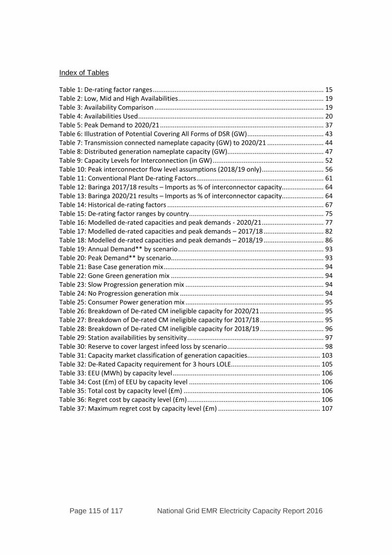
Page 115 of 117 National Grid EMR Electricity Capacity Report 2016
Index of Tables
Table 1: De-rating factor ranges.............................................................................................. 15Table 2: Low, Mid and High Availabilities................................................................................ 19Table 3: Availability Comparison ............................................................................................. 19Table 4: Availabilities Used...................................................................................................... 20Table 5: Peak Demand to 2020/21.......................................................................................... 37Table 6: Illustration of Potential Covering All Forms of DSR (GW).......................................... 43Table 7: Transmission connected nameplate capacity (GW) to 2020/21 ............................... 44Table 8: Distributed generation nameplate capacity (GW)..................................................... 47Table 9: Capacity Levels for Interconnection (in GW)............................................................. 52Table 10: Peak interconnector flow level assumptions (2018/19 only).................................. 56Table 11: Conventional Plant De-rating Factors...................................................................... 61Table 12: Baringa 2017/18 results – Imports as % of interconnector capacity....................... 64Table 13: Baringa 2020/21 results – Imports as % of interconnector capacity....................... 64Table 14: Historical de-rating factors ...................................................................................... 67Table 15: De-rating factor ranges by country.......................................................................... 75Table 16: Modelled de-rated capacities and peak demands - 2020/21.................................. 77Table 17: Modelled de-rated capacities and peak demands – 2017/18 ................................. 82Table 18: Modelled de-rated capacities and peak demands – 2018/19 ................................. 86Table 19: Annual Demand** by scenario................................................................................ 93Table 20: Peak Demand** by scenario.................................................................................... 93Table 21: Base Case generation mix........................................................................................ 94Table 22: Gone Green generation mix .................................................................................... 94Table 23: Slow Progression generation mix ............................................................................ 94Table 24: No Progression generation mix ............................................................................... 94Table 25: Consumer Power generation mix ............................................................................ 95Table 26: Breakdown of De-rated CM ineligible capacity for 2020/21 ................................... 95Table 27: Breakdown of De-rated CM ineligible capacity for 2017/18 ................................... 95Table 28: Breakdown of De-rated CM ineligible capacity for 2018/19 ................................... 96Table 29: Station availabilities by sensitivity........................................................................... 97Table 30: Reserve to cover largest infeed loss by scenario..................................................... 98Table 31: Capacity market classification of generation capacities........................................ 103Table 32: De-Rated Capacity requirement for 3 hours LOLE................................................. 105Table 33: EEU (MWh) by capacity level................................................................................. 106Table 34: Cost (£m) of EEU by capacity level ........................................................................ 106Table 35: Total cost by capacity level (£m) ........................................................................... 106Table 36: Regret cost by capacity level (£m)......................................................................... 106Table 37: Maximum regret cost by capacity level (£m) ........................................................ 107

Page 116 of 117 National Grid EMR Electricity Capacity Report 2016
Copyright © 2016 National Grid
All rights reservedNational Grid plcNational Grid HouseWarwick Technology ParkGallows HillWarwickCV34 6DA
http://www2.nationalgrid.com
