national medical expenditure survey with the national · expenditure survey with the national ......

Design Alternativesfor Integrating theNational MedicalExpenditure SurveyWith the NationalHealth InterviewSurveyResearch was undertaken to evaluate

alternative methods of selecting a sample

of eligible respondents for the National

Medical Expenditure Survey (NM ES) from

the National Health Interview Survey

(N HIS). This report presents estimates of

the effects of alternative design options,

obtained by statistical modeling

techniques, for linking the NMES with the

NH IS, The estimated survey costs for

alternative linked and unlinked design

options are compared for fixed precision.

The findings indicate that substantial

savings would be realized by linking the

NMES to the NHIS if a premium is put on

small-domain estimates.

Data Evaluation and Methods ResearchSeries 2, No. 101

DHHS Publication No. (PHS) 87–1375

U.S. Department of Health and Human

Services

Public Health Service

National Center for Health Statistics

Hyattsville, Md.

March 1987

Copyright information

All material appearing inthla report is Inthepubltc domatn and may

be reproduced or copied without permission; citation as to source,

however, is appreciated.

Suggested citation

National Center for Health Statistics, B. G. COX, R E. Folsom, T, G. Vlrag:

Design alternatives forintegrating the National Med!cal Expenditure

Survey With the National Health /ntewiew Suwey. Series2, No, 101,

DHHS Pub. No. 87-1375, Public Health Service. Washington. U.S.

Government Printing Office, Mar. 1987.

Libratyof Congress Cataloging-in-Publication Data

Cox, Brenda G

Design alternatives forintegratlng the National

Medical Expenditure Survey with the National Health

Interview Survey,

(Series 2, Data evaluation and methods research ;

no. 101) (DHHS publication ; no. (PHS) 87–1 375)

Written by Brenda G, Cox, Ralph E. Fulsom, Thomas

G, Virag.

“August 1986. ”

Bibliography p.

Supt. of dots. no.: HE20.6209:2/l 01

1. Medical care, Cost of—lJnited States— S?atlstlcal

methods. 2. Medical care—United States— Utillzation—

Statistical methods, 3. Health surveys-United States

4. National Health Interview Survey (U. S.) 5. National

Medical Expenditure Survey (U. S.) 1. Folsom, Ralph E.

Il. Virag, Thomas G, Ill, National Center for Health

Statistics (U. S.} IL. Title, V. Vital and health

statistics. Ser!es 2, Data e,Jaluation and methods

research ; no. 101 VI, Series: DHHS public attofi ;

no. (PHS) 87–1 375. [DNLM: 1. Data Collection—statistics

2. Health Surveys-United States—statistics. 3 Iriforma.

tion Systems—statistics, W2 A N1 48vb no. 101 j

RA409. U45 no. 101 362.1 ‘0723 S 86–600233

[RA407.3] [362.1 ‘0973]

ISBN 0–8406–0343–6

National Center for Health Statistics

Manning Feinleib, M.D., Dr. P.H., Director

Robert A. Israel, Deputy Director

Jacob J. Feldman, Ph.D., Associate Director for Analysisand Epidemiology

Gail Fisher, Ph.D., Associate Director for Planning andExtramural Programs

Peter L. Hurley, Associate Director for Vital and HealthStatistics Systems

Stephen E. Nieberding, Associate Director for Management

George A. Schnack, Associate Director for Data Processingand Services

Monroe G. Sirken, Ph.D., Associate Director for Researchand Methodology

Sandra S. Smith, Information Oficer

Office of Research and Methodology

Monroe G. Sirken, Ph.D., Associate Director

Kenneth W. Harris, Special Assistant for ProgramCoordination and Statistical Standards

Lester R Curtin, Ph.D., Acting ChieJ Statistical MethodsStafl

James T. Massey, Ph.D., Chiex Survey Design Stafl

Foreword

This is the second report presenting results of research onthe effects of integrating the designs of the National Center forHealth Statistics (NCHS) national household sample surveys,which heretofore were designed as independent surveys. Designintegration would be accomplished by using the fdes of theNational Health Interview Survey (NHIS), the largest and onlycontinuing NCHS population survey, as the sampling framefor NCHS’S other population surveys. Research findings withrespect to linking the 1987 National Survey of Family Growth(NSFG) to NHIS were presented in an earlier report in thispublication series, and the fiidings relating to the 1987 Na-tional Medical Expenditure Survey (NMES) are presented inthk report.

The earlier report indicated that significant economieswould be realized by linking NSFG to NHIS because NSFGrequires a substantial oversrunpling of households with blackfemales. However, it was unreasonable to assume that the

NSFG findings would necessarily apply to NMES becauseNSFG is a single-time retrospective survey and NMES is apanel survey. As such tie population domains of interest wouldbe different for NMES and NSFG. As it turned out, theNMES and NSFG research findingswere quite similar. Amongother things, this report concludes that substantial savings wouldbe realized by linkingNMES to NHIS ifNMES puts a premiumon small-domain estimates.

I provided technical oversight to this project which wasconducted under a contract with the Research Triangle Insti-tute. Dr. Andrew White was instrumental in guiding this reportthrough the publication process by working closely with theauthors and the editors.

Monroe G. SirkenAssociate Director for Research and Methodology

.Ill

Symbols

--- Data not available

. . . Categov not applicable

Quantity zero

0.0 Quantity more than zero but less than

0.05

z Quantity more than zero but less than

500 where numbers are rounded to

thousands

* Figure does not meet standard of

reliability or precision

# Figure suppressed to comply with

confidentiality requirements

iv

Chapter 1, Introduction . . . . . . . . . . . . . . . . . . . . . . . . . . . . . . . . . . . . . . . . . . . . . . . . . . . . . . . . . . . . . . . . . . . . . . . . . . . . . . . . . . . . .

Chapter 2. The unlinked National Medical Expenditure Survey . . . . . . . . . . . . . . . . . . . . . . . . . . . . . . . . . . . . . . . . . . . . . . . . . . .Definition . . . . . . . . . . . . . . . . . . . . . . . . ...!.. . . . . . . . . . . . . . . . . . . . . . . . . . . . . . . . . . . . . . . . . . . . . . . . . . . . . . . . . . . . . . . . . .Sample size determination . . . . . . . . . . . . . . . . . . . . . . . . . . . . . . . . . . . . . . . . . !, . . . . . . . . . . . . . . . . . . . . . . . . . . . . . . . . . . . . . .Variance modeling . . . . . . . . . . . . . . . . . . . . . . . . . . . . . . . . . . . . . . . . . . . . . . . . . . . . . . . . . . . . . . . . . . . . . . . . . . . . . . . . . . . . ...!Cost modeling . . . . . . . . . . . . . . . . . . . . . . . . . . . . . . . . . . . . . . . . . . . . . . . . . . . . . . . . . . . . . . . . . . . . . . . . . . . . . . . . . . . . . . . . . . .Other design considerations . . . . . . . . . . . . . . . . . . . . . . . . . . . . . . . . . . . . . . . . . . . . . . . . . . . . . . . . . . . . . . . . . . . . . . . . . . . . . . . .

Tables

1. Completed reporting unit interviews by round for the unlinked designs with 6,000- and 10,OOO-respondentoriginatingbasereporting units . . . . . . . . . . . . . . . . . . . . . . . . . . . . . . . . . . . . . . . . . . . . . . . . . . . . . . . . . . . . . . . . . . . . . . . . . . . . . . . . . . .

2, Proportions of National Medical Care Utilization and Expenditure Survey expenditures and utilization variation bydomain sndtype of service . . . . . . . . . . . . . . . . . . . . . . . . . . . . . . . . . . . . . . . . . . . . . . . . . . . . . . . . . . . . . . . . . . . . . . . . . . . . .

3. Estimated means and relative standard errors for the unlinked National Medical Expenditure Survey design with6,000- and 10,OOO-respondentoriginating base reporting units . . . . . . . . . . . . . . . . . . . . . . . . . . . . . . . . . . . . . . . . . . . . . . .

4, Summary of estimated costs of project tasks for the 6,000-respondent originating base reporting unit unlinked design . . .5. Summary of estimated costs of project tasks for the 10,OOO-respondentoriginating base reporting unit unlinked design. . .6. Overview of Research Triangle Institute (RTI) and National Opinion Research Center actual National Medical Care

Utilization and Expenditure Survey (NMCUES) Household Survey direct cost experience compared with a 1980NMCUESRTI-only design . . . . . . . . . . . . . . . . . . . . . . . . . . . . . . . . . . . . . . . . . . . . . . . . . . . . . . . . . . . . . . . . . . . . . . . . . . . .

Chapter 3, Thelinked dwelling unitdesign.. . . . . . . . . . . . . . . . . . . . . . . . . . . . . . . . . . . . . . . . . . . . . . . . . . . . . . . . . . . . . . . . . . . .Definition . . . . . . . . . . . . . . . . . . . . . . . . . . . . . . . . . . . . . . . . . . . . . . . . . . . . . . . . . . . . . . . . . . . . . . . . . . . . . . . . . . . . . . . . . . . . . . .Sample sizedetermination . . . . . . . . . . . . . . . . . . . . . . . . . . . . . . . . . . . . . . . . . . . . . . . . . . . . . . . . . . . . . . . . . . . . . . . . . . . . . . . . .Cost modeling . . . . . . . . . . . . . . . . . . . . . . . . . . . . . . . . . . . . . . . . . . . . . . . . . . . . . . . . . . . . . . . . . . . . . . . . . . . . . . . . . . . . . . . . . . .Other design considerations .. 0..,.. . . . . . . . . . . . . . . . . . . . . . . . . . . . . . . . . . . . . . . . . . . . . . . . . . . . . . . . . . . . . . . . . . . . . . . . .

Tables

7. Required segment size for the linked design to obtain the precision of the unlinked design by domain and type of service . . .8, Summary of estimated costs of project tasks for linked dwelling unit design A . . . . . . . . . . . . . . . . . . . . . . . . . . . . . . . . . .9, Summary of estimated costs of project tasks for linked dwelling unit design B. . . . . . . . . . . . . . . . . . . . . . . . . . . . . . . . . . .

10. Summary of estimated costs of project tasks for linked dwelling unit design C . . . . . . . . . . . . . . . . . . . . . . . . . . . . . . . . . .11, Summary of estimated costs of project tasks for linked dwelling unit design D . . . . . . . . . . . . . . . . . . . . . . . . . . . . . . . . . .

Chapter 4. Thelinked household design . . . . . . . . . . . . . . . . . . . . . . . . . . . . . . . . . . . . . . . . . . . . . . . . . . . . . . . . . . . . . . . . . . . . . . .Definition . . . . . . . . . . . . . . . . . . . . . . . . . . . . . . . . . . . . . . . . . . . . . . . . . . . . . . . . . . . . . . . . . . . . . . . . . . . . . . . . . . . . . . . . . . . . . . .Sample size determination . . . . . . . . . . . . . . . . . . . . . . . . . . . . . . . . . . . . . . . . . . . . . . . . . . . . . . . . . . . . . . . . . . . . . . . . . . . . . . . . .Costmodeling . . . . . . . . . . . . . . . . . . . . . . . . . . . . . . . . . . . . . . . . . . . . . . . . . . . . . . . . . . . . . . . . . . . . . . . . . . . . . . . . . . . . . . . . . . .Other design considerations . . . . . . . . . . . . . . . . . . . . . . . . . . . . . . . . . . . . . . . . . . . . . . . . . . . . . . . . . . . . . . . . . . . . . . . . . . . . . . . .

Tables

12, Sample sizes for the 1980 National Medical Care Utilization and Expenditure Survey design . . . . . . . . . . . . . . . . . . . . .13. Sample sizes for the National Medical Expenditure Survey linked household design . . . . . . . . . . . . . . . . . . . . . . . . . . . . .14, Summ~ofestimated costs ofproject tasks forlhked household desire A . . . . . . . . . . . . . . . . . . . . . . . . . . . . . . . . . . . . .

1

222355

7

8

101214

16

1717171819

2022

242628

3030303032

333334

v

15. Summery of estimated costs of project tasks for linked household design B . . . . . . . . . . . . . . . . . . . . . . . . . . . . . . . . . . . . . 3616. Summary of estimated costs of project tasks for linked household design C17.

. . . . . . . . . . . . . . . . . . . . . . . . . . . . . . . . . . . . .Summary of estimated costs of project tasks for linked household design D . . . . . . . . . . . . . . . . . . . . . . . . . . . . . . . . . . . . .

Chapter 5. An optimally allocated design . . . . . . . . . . . . . . . . . . . . . . . . . . . . . . . . . . . . . . . . . . . . . . . . . . . . . . . . . . . . . . . . . . . . . .Definition . . . . . . . . . . . . . . . . . . . . . . . . . . . . . . . . . . . . . . . . . . . . . . . . . . . . . . . . . . . . . . . . . . . . . . . . . . . . . . . . . . . . . . . . . . . . . . .Variance modeling . . . . . . . . . . . . . . . . . . . . . . . . . . . . . . . . . . . . . . . . . . . . . . . . . . . . . . . . . . . . . . . . . . . . . . . . . . . . . . . . . . . . . . . .Cost modeling . . . . . . . . . . . . . . . . . . . . . . . . . . . . . . . . . . . . . . . . . . . . . . . . . . . . . . . . . . . . . . . . . . . . . . . . . . . . . . . . . . . . . . . . . . .Optimization results . . . . . . . . . . . . . . . . . . . . . . . . . . . . . . . . . . . . . . . . . . . . . . . . . . . . . . . . . . . . . . . . . . . . . . . . . . . . . . . . . . . . . .Other design considerations . . . . . . . . . . . . . . . . . . . . . . . . . . . . . . . . . . . . . . . . . . . . . . . . . . . . . . . . . . . . . . . . . . . . . . . . . . . . . . . .

Tables

18. Sample sizes for the alternate optimally allocated designs . . . . . . . . . . . . . . . . . . . . . . . . . . . . . . . . . . . . . . . . . . . . . . . . . . .19. Stratum sampling rates for the alternate optimally allocated designs . . . . . . . . . . . . . . . . . . . . . . . . . . . . . . . . . . . . . . . . . . .20. Stratum originating base reporting unit sample sizes for the alternate optimally allocated designs . . . . . . . . . . . . . . . . . .

Chapter 6. Comparison of the designs and recommendations . . . . . . . . . . . . . . . . . . . . . . . . . . . . . . . . . . . . . . . . . . . . . . . . . . . . . .

Table

21. Sample size summary for the alternate National Medical Expenditure Survey design . . . . . . . . . . . . . . . . . . . . . . . . . . . .

References . . . . . . . . . . . . . . . . . . . . . . . . . . . . . . . . . . . . . . . . . . . . . . . . . . . . . . . . . . . . . . . . . . . . . . . . . . . . . . . . . . . . . . . . . . . . . . . .

Appendix. Description of cost modeling process . . . . . . . . . . . . . . . . . . . . . . . . . . . . . . . . . . . . . . . . . . . . . . . . . . . . . . . . . . . . . . . .

Tables

I. Summary of Research Triangle Institute cost experience for survey sampling for the National Medical Care Utilizationand Expenditure Survey Household Survey by month . . . . . . . . . . . . . . . . . . . . . . . . . . . . . . . . . . . . . . . . . . . . . . . . . . . . . .

II. Summary of Research Triangle Institute cost experience for survey sampling for the National Medical Care Utilizationand Expenditure Survey Household Survey, rounds 1–5 . . . . . . . . . . . . . . . . . . . . . . . . . . . . . . . . . . . . . . . . . . . . . . . . . . .,

III. Summary of Research Triangle Institute cost experience in percent for survey sampling for the National MedicalCare Utilization and Expenditure Survey Household Survey, rounds 1–5 . . . . . . . . . . . . . . . . . . . . . . . . . . . . . . . . . . . . . .

IV. Summary of Research Triangle Institute cost experience for survey sampling for the National Medical Care Utilizationand Expenditure Survey Household Suwey, rounds 1–5, by type of cost

v.. . . . . . . . . . . . . . . . . . . . . . . . . . . . . . . . . . . . . .

Summary of estimated costs for survey sampling with the Research Triangle Institute design component of the 1980NMCUES . . . . . . . . . . . . . . . . . . . . . . . . . . . . . . . . . . . . . . . . . . . . . . . . . . . . . . . . . . . . . . . . . . . . . . . . . . . . . . . . . . . . . . . . . . .

VI. Summary of estimated costs for survey sampling with the 6,000-respondent originating base reporting unit unlinkeddesign . . . . . . . . . . . . . . . . . . . . . . . . . . . . . . . . . . . . . . . . . . . . . . . . . . . . . . . . . . . . . . . . . . . . . . . . . . . . . . . . . . . . . . . . . . . . . . .

VII. Summary of estimated costs for survey sampling with the 10,OOO-respondentoriginating base reporting unit unlinkeddesign . . . . . . . . . . . . . . . . . . . . . . . . . . . . . . . . . . . . . . . . . . . . . . . . . . . . . . . . . . . . . . . . . . . . . . . . . . . . . . . . . . . . . . . . . . . . . . .

VIII. Summary of costs for survey sampling for the linked household design. . . . . . . . . . . . . . . . . . . . . . . . . . . . . . . . . . . . . . . . .IX. Summary of estimated costs for survey sampling for the linked household design A..... . . . . . . . . . . . . . . . . . . . . . . . . .x. Summary of estimated costs for survey sampling for the linked household design B . . . . . . . . . . . . . . . . . . . . . . . . . . . . . .XI. Summary of estimated costs for survey sampling for the linked household design C . . . . . . . . . . . . . . . . . . . . . . . . . . . . . .XII. Summary of estimated costs for survey sampling for the linked household design D. . . . . . . . . . . . . . . . . . . . . . . . . . . . . .

3840

424243444546

484848

49

51

52

53

54

55

56

58

60

62

646668707274

vi

Design Alternatives forIntegrating the NationalMedical Expenditure SurveyWith the National HealthInterview Surveyby Brenda G. Cox, Ralph E. Foisom, and Thomas G. Virag,

Research Triangle Institute

Chapter 1Introduction

Current planning for population-based surveys conductedby the National Center for Health Statistics (NCHS) suggeststhat the data systems can be integrated to save on data collec-tion costs, to reduce respondent burden, and to increase theutility of the resultant data. As part of the NCHS effort to

evaluate advantages of an integrated data system, ResearchTriangle Institute examined alternative designs for integratingthe National Medical Expenditure Survey (NMES) with thelarger National Health Interview Survey (NHIS). NMES willbe a longitudinal study of the 1987 health care utilization andexpenditures of civilian noninstitutionalized residents of theUnited States. This report summarizes the results of an in-vestigation to assess the feasibility of linking the two surveys.

As a baseline for comparison, specifications for an unlinkedNMES design were developed Selected independently of NHIS,this unlinked design results in a stratified clustered area samplesimilar to that of the 1980 National Medical Care Utilizationand Expenditure Survey. For flexibility of NCHS planning,two sample sizes were used 6,000 and 10,000 respondinghouseholds. The 6,000-household design is similar in size tothe 1980 National Medical Care Utilization and ExpenditureSurvey. The 10,OOO-householddesign was added so that NCHScould evaluate the improved precision for surveying smallerdomains with the larger sample against the increased surveycost, Survey costs for the two sample size alternatives weremodeled as well as the variances for selected statistics of in-terest.

The second design for which specifications were developedwas a linked dwelling unit design. The linked dwelling unitdesign selects the sample of individuals to be included inNMES by subsampling NHIS sample dwelling units. In round1 of NMES, the occupants of the subssmpled dwelling unitswould be interviewed. Rounds 2–5 of date collection woulduse the same procedures as the unlinked NMES design. Tomeasure the effect of the number of NHIS primary samplingunits (PSU’S) from which the NMES sample dwelling units areselected, both a 1OO-PSU and a 200-PSU linked dwelling unitdesign were investigated. For each design, two sample sizealternatives were also investigated. These two sample sizes arethose required to yield the same precision as the unlinked designwith 6,000 and 10,000 responding households.

The third set of specifications developed were for a linkedhousehold design. The linked household design selects a sampleof NHIS households for inclusion in NMES. The individualswithin the subsampled households are interviewed in round 1whether or not they live in the clustered NHIS sample dwellingunits. Rounds 2–5 data collection uses the same rules as theunlinked design. As in the linked dwelling unit design, to assessthe effect of the number of PSU’S, designs were developed forboth 100 PSU’S and 200 PSU’S; two sample sizes were in-vestigated. These sample sizes were determined as the sizesrequired to yield the same precision as the unlinked design with6,000 and 10,000 responding households.

Each of these designs is self-weighting that is, all sampleindividuals are selected with the same probability. In manyways this eliminates the chief advantage of linkage with NHIS.With knowledge of individual characteristics available forNHIS sample respondents, added precision can be obtainedfor small domains without proportionally increasing the size ofthe total sample. To evaluate this feature of NHIS linkage, afourth and final design type was investigated. This design is anoptimally allocated linked household design in which the pre-cision constraints set for the total population and the Medicaidpopulation were based on those achieved by the unlinked design.Instead of arbitrarily determining the number of NHIS PSU’Sand segments to include, optimal sizes were determined forthese components.

The development of these four designs is described in thefollowing chapters, An important finding of this investigation isthat there appears to be little relative gain from linkage whenthe final design is self-weighting. The principal gain from thelinked self-weighting design is in the elimination of costs as-sociated with counting and listing. Because the NMCUESinterview pattern for all rounds was adopted in this investiga-tion (personal interviews are used in the first two rounds andtelephone interviews in the third and fourth rounds), there islittle gained from the names, addresses, and telephone numbersof NHIS sample individuals. The optimrdly allocated design,however, uses characteristics of NHIS respondents to over-simple heavy users of health care services and to increase theprecision for small domains without proportionally increasingthe size of the total sample.

1

Chapter2The unlinked NationalMedical ExpenditureSurvey design

The unlinked National Medical Expenditure Survey(NMES) designs studied in this investigation were patternedafter the design used for the 1980 National Medical CareUtilization and Expenditure Survey (NMCUES), Specifically,an area sampling approach was used incorporating a self-weighting design in which each sample individual is selectedwith equal probability. The srunple sizes required to yield6,000 and 10,000 responding households were determined aswell as the survey costs associated with these designs. Thevariances achieved by the unweighed, unlinked NMES designwere modeled for use in sample size determination for the re-maining designs,

Definition

The unlinked sample design is a stratified, multistage areaprobability design in which each sample dwellingunit is selectedwith equal probability. (In this report, the term “dwelling unit”refers to either a housing unit or a group quarters listing unit.)The first-stage sample consists of primary sampling units(PSU’S) that are counties, parts of counties, or groups of con-tiguous counties. The second-stage sample consists of secondarysampling units that are census enumeration districts or blockgroups. Smaller area segments constitute the third stage. All ofthe dwelling units within these sample segments are listed.During the fourth stage of sampling, dwelling units within thesesample segments are designated for inclusion in the NMESsample.

All civilian noninstitutionalized individuals residing in thesampled dwelling units in round 1 are included in the survey.Single college students in the 17–22-year age range are linkedto their parents’ residence and included in the survey onlywhen their parents’ residence is selected. Round 1 data collec-tion uses personal interviews except for college students livingoutside a 2-hour, one-way drive of a sample PSU. In this case,telephone interviewing is used.

In round 2, these key persons are interviewed in theirround 2 location. Individuals and families that moved must betraced to determine their new addresses. Individuals who joinedthe family of a key individual by birth or return from an institu-tion, the military, or an overseas residence are included inNMES as a key person. Other individuals joining the familiesof key persons are classified as nonkey. Data are collected forboth key and nonkey persons. The data for key persons areneeded for person-level analyses. The data for nonkey personsare needed for family-level analyses only. Data collection inround 2 also uses personal interviews except for college stu-

dents and movers outside a 2-hour, one-way drive from asample PSU.

In round 3, data collection is primarily by telephone, withpersonal interviews conducted only for households withouttelephones and households requesting personal interviews.Key persons who move from their round 2 locations must betraced and interviewed at their new locations. Nonkey personswho moved are interviewed only when a key person moveswith them. Individuals who are born or who return from aninstitution, the militaxy, or overseas residence are included askey persons. Other individuals joining the families of key per-sons are classified as nonke~ data are gathered for them onlyduring the time in which they were members of a key person’sfamily.

The mode of data collection in round 4 follows that ofround 3 with similar guidelines for key and nonkey persons.Because December 31 is the end of the survey reference period,approximately 30 percent of the sample is not interviewed inround 4 but instead early in round 5 (that is, shortly after Jan-uary 1 of the next year).

The final round of data collection primarily uses personalinterviewing under the same guidelines used in previous roundsto define key and nonkey persons and to determine movers whowill be followed.

Sample size determination

Two sets of sample sizes were required for the unlinkedNMES desigm A sample size sufficient to yield 6,000 respond-ing households, and a sample size sufficient to yield 10,000responding households, To obtain these sizes, a precise defini-tion was needed for “responding household.” It was decided touse responding originating base reporting units (OBRU’S) andto describe the sample sizes needed as those yielding an OBRUdesign with 6,000 responding and an OBRU design with 10,000responding. These OBRU’S are the round 1 reporting units(RU’S) after college student RU’S are linked back to parentRU’S. Because data collection costs relate to reporting units(RU’S) and rounds, sample sizes in terms of these units weredeveloped.

The f~st step in this process was to model the 1980NMCUES experience starting with the set of control systemrecords generated by responding OBRU’S. (In the NMCUES,an OBRU was defined to be responding if it was linked to anRU that completed an interview in any of the five data collec-tion rounds.) The NMCUES contained 6,269 respondingOBRU’S. These responding OBRU’S generated 6,603 com-

2

pleted RU interviews in round 1, 6,519 completed RU inter-views in round 2, 6,528 completed RU interviews in round 3,4,559 completed RU interviews in round 4, and 6,561 com-pleted RU interviews in round 5. These were more RU inter-views than there were responding OBRU’S because OBRU’Scontaining college students required more than one RU assign-ment to handle the different addresses at which data collectionoccurred, The NMCUES intexwiewsoccurred in 135 PSU’Sand 809 segments.

Because the NMES should experience no worse than thenonresponse and attrition encountered by the 1980 NMCUES,the NMCUES experience was ratio adjusted to produce thesample sizes required for the OBRU designs with 6,000 and10,000 responding. These sample sizes are summarized intable 1, For modeling convenience, it was assumed that theResearch Triangle Institute (RTI) General Purpose Samplewould be used, which contains 102 PSU’S. The average seg-ment size was set to the 1980 NMCUES experience of eightresponding OBRU’S. With eight responding OBRU’S per seg-ment, the OBRU design with 6,000 responding would require750 segments, and the OBRU design with 10,000 respondingwould require 1,250 segments.

Variance modeling

As a baseline for comparison of the unlinked with the linkeddesigns, the precision of the linked designs was fixed to that ofthe unlinked design for selected key statistics and key domains.The designs were then compared with respect to sample sizesand costs. The domains of interest were the total population,those individuals below 150 percent of poverty, Medicare re-cipients, Medicaid recipients, and individuals from familieswith college-educated heads of households. The statistics ofinterest were as follows:

●

●

●

●

●

s

●

●

●

●

Average number of hospital visits.Average number of facility visits.Average number of ofice visits.Average annual expenditure for hospital visits.Average annual expenditure for facility visits.Average annual expenditure for ofiice visits.Average annual out-of-pocket expense for hospital visits.Average annual out-of-pocket expense for facility visits.Average annual out-of-pocket expense for ofilce visits.Proportion with large out-of-pocket expenditures.

To determine the sample sizes required for the linked designs,the variance was modeled for the OBRU unlinke~ self-weightingdesigns with 6,000 and 10,000 responding using the 1980NMCUES data.

The NMES estimation approach constructs means in termsof total person-years rather than in terms of all persons everexisting in the data collection year, For domain lG the meanutilizationor expenditureper person-yearis estimatedas

~ w(i)l$k(z-)Y(i)

Yk(NMES) = ‘es~W(i)T(i)c$k(i) (1)

iES

where W(i) = analysis weight for the ith person

d~(i) = 1 if the ithperson belongs to the kth domain andO if not

Y(i) = response of the ith person

T(i) = time-adjustmentfactor for the ith person

The numerator estimates total expenditures or utilization andthe denominator the average annual number of persons in thepopulation (that is, the total person-years). The time-adjustmentfactor T(i) is the total days that person i is eligible divided bythe number of days in the year.

Large out-of-pocket expenditures are defined as “annual-ized” out-of-pocket expenditures of $200 or more. The armual-ized out-of-pocket expenditure is the annual out-of-pocket ex-penditure divided by the fraction of the year during which theperson is eligible. For domain ~ the proportion with large out-of-pocket expenditures is estimated as

where Y(i) = 1 if the person had large out-of-pocket expendi-tures and Oif not.

The variables used in constructing these estimates wereinterim variables ffom the NMCUES analysis ffles and not thefinal variables contained in the public use fdes. For this reason,the estimates in this report may differ horn those in otherNMCUES reports.

The variance of ~k(NMES) was derived assuming a three-stage household survey design patterned after the 1980NMCUES sample design with PSU’S of standard metropolitanstatistical areaj or county-size and area segments (SEG’S)selected as noncompact clusters of dwelling units. The house-holds containing at least one RU response are designated asresponding OBRU’S. Using this approach, the variance of~~(NMES) maybe modeled as

where dk(PSU) = between-PSU, within-stratum variance com-ponent for domain k

r = number of PSU’S

a~(SEG) = between-segment,within-PSU variance com-ponent for domain k

F= average number of segments per PSU

~(OBRU) = between-OBRU, within-segment variancecomponent for domain k

7’= average number of responding OBRU’S persegment

3

The variance components were estimated using 1980NMCUES data.

The variance components estimation program, developedat RTI by Shah* for evaluating the efficiency of complex sampledesigns, was applied to the NMCUES data to produce thegeneralized composite components for PSU’S, segments(SEG’S), and OBRU’S. VMCPNLS estimates the compositevariance components in terms of an expression for the varianceof a multistage Horvitz-Thompson estimator derived by Gray.2For the NMCUES design, VMCPNLS yields a four-stageanalysis including a between-PSU component [~#PSU)]; abetween-segment, within-PSU component [~~(SEG)]; a be-tween-OBRU, within-segment component [~#(OBRU)]; anda between-person (PID), within-OBRU component [~~PID)].

Because there is no subsampling of household members inNMCUES, the four-stage decomposition produced byVMCPNLS must be converted to the three-stage decomposi-tion spec~led in equation (3). With the four-stage model, thePSU and segment components are equivalent to the corre-sponding parameters of the three-stage model. The OBRU-level component can be estimated from the four-stage com-ponents as ~~(OBRU) + ~~(PID)/E where n is the averagenumber of responding persons per responding OBRU. Usingthe 1980 NMCUES data, ii is estimated to be 2.73.

The variance components estimated using the 1980NMCUES data contain an effect due to unequal weighting ofthe NMCUES sample. To remove the unequal weighting effect,these components were converted to the variance proportionsAk(PSU), AJSEG), and A~(OBRU) by dividing by the totalvariation or

h )Psu

AJPSU) = :

~(TOT)k

3( )SEG

Ak(SEG) = :

~(ToT)k

(4)

(5)

2 2

~mw + ~(pID)/z

Ak(OBRU) = k , k (6)

~(ToT)k

where ~~(TOT) is defined as

&mv=&w.o+~(SEG) +&OBRu)k k k k

+k ii (7)

Table 2 displays these variance proportions for the 5 domainsof interest and the 10 outcome measures described earlier.

To obtain the & variance components used in modelingthe variance of the key statistics, the variance proportions weremultiplied by the estimated population variance for the kthdomain, denoted by S2(k). That is,

c$(PSU) = Ak(PSv~2(k) (8)

~(SEG) = Ak(SEG)S2(k) (9)

~(OBRU) = Ak(OBRU)~2(k) (lo)

A Taylor series approximation for the simple random samplingvariance of a combined ratio estimator was used to estimate5’2(k). The numerator was the Y total for domain k and thedenominator the total person-years for domain k (See equa-tions (1) and (2).)

These three-stage variance component estimates were usedto estimate the variances that would be achieved by self-weight-ing NMES OBRU designs with 6,000 and 10,000 responding.The terms remaining to be specified in the variance expressionpresented in equation(3) are the number of PSU’S, r; the averagenumber of segments sampled per PSU, F and the averagenumber of OBRU’S sampled per segment, Z For modeling pur-poses, the RTI’s General Purpose Sample was assumed, whichcontains 102 PSU’S (r= 102). Because the 1980 NMCUEShad been designed to be optimal with respect to the number ofselections per segment, the number of responding OBRU’S persegment was set to the value that the 1980 NMCUES achieved,or~= 8. Therefore, the total number of segments in the OBRUdesign with 6,000 responding would be 750 (r~ = 750) and1,250 for the OBRU designwith 10,000 responding(R = 1,250),

These estimated variances were used as precision criteriafor the other designs investigated in this study. Table 3 presentsthe results of this variance modeling activity for the 5 domainsof interest and the 10 outcome measures, For convenience,percent relative standard errors are used rather than the vari-ances. The percent relative standard error is 100 times thestandard error (the square root of the variance) divided by theparameter being estimated. The percent relative standard errorsachieved by the OBRU design with 6,000 responding are suf-ficient for the estimates based upon the total domain, but theincreased precision that the OBRU design with 10,000 re-sponding achieves for the small domain estimates is desirable.

Cost modeling

To establish cost comparisons between the unlinked andthe linked designs, a systematic method was developed to gen-erate.the costs for all designs. The approach used was to developunit costs by task for each design. The NMES tasks includedin the modeling were the basic sampling and weighting tasksand the data collecting and processing tasks:●

●

●

●

●

●

●

●

●

●

●

●

●

●

●

Survey sampling,Instrument and materials development.Field preparations.Survey training.Data collection.Control system development and production.Data receipt, editing and document control.Data coding operations.Data entry operations.Control card development, maintenance, and production.Summary development, maintenance, and production.Other data processing operations.Database construction.Counting and listing,Project administration.

The unit costs that were developed for each task were f~edcosts, PSU-level costs, segment-level costs, and reporting-unit-level costs.

The first step in the process was to document the RTI costexperience for the 1980 NMCUES. Because of insufficientdata for other contractors’ costs, modeling was conducted withonly RTI data, Only direct costs were included in the modelingbecause indirect costs, such as the costs for administration andbuilding maintenance, vary among contractors as do accountingprocedures used to recover these costs. Another step in doc-umenting RTI costs for NMCUES was to separate the NationalHousehold Survey (HHS) costs from the costs associated withthe four State Medicaid Household Surveys (SMHS). In mostcases, SMHS activity was conducted under task numbers dif-ferent fi’omthe HHS. In situations where HHS data and SMHSdata were processed simultaneously, the additional costs addedby SMHS were removed.

The next step was to use the 1980 NMCUES cost experi-ence to develop unit costs for each task. Derivation of the unitcosts by NMES task was a time-consuming process. The appendix includes a discussion of this process. The results aresummarized in tables 4 and 5. Table 4 presents the costs for

the OBRU design with 6,000 responding by category of costfor each of the 15 NMES tasks. Table 5 presents the costs forthe OBRU design with 10,000 responding. For the OBRU de-sign with 6,000 responding, direct costs are $4,963,013. Forthe OBRU design with 10,000 responding, direct costs are$7,209,409.

Other design considerations

Data for the 1980 NMCUES were collected by two con-tractors: RTI and the National Opinion Research Center(NORC), The cost modeling presented in this chapter wasbased on data from one contractor, however. There are ad-

vantages and disadvantages associated with using more thanone contractor in data collection. These differences includequality, timeliness, and cost considerations.

Whether the OBRU design with 10,000 responding ischosen over the OBRU design with 6,000 responding, NMESwill have time constraints on data collecting and processing,because data collection rounds are approximately 3 monthsapart. In the time between rounds 2 and 3, for instance, thedata for round 2 must be collected, keyed, edited, coded, andentered into the database. The database is then used to gen-erate a cumulative summary of household health care utilizationand expenditures. This summary must be mailed to each house-hold and interviewer before round 3. The volume of data col-lecting and processing required in this limited timeframe isbeyond the capability of all but the largest fins. Hence, manyfirms would need to work together to accomplish the task.

Another advantage of using more than one contractor isthe potential for improvements in work quality. Access to ex-perienced interviewing and supervisory staff is limited to thevolume of work performed. The inhouse staff needed to monitordata collection, to edit and to key the dat~ and to produce thefinal database is also limited. Merging the resources of morethan one contractor enlarges the pool of experienced staff whocan be assigned to a task.

The disadvantage of using more than one contractor is theinevitable duplication of effort. Each organization incurs thefixed costs associated with sampling, data collection, and dataprocessing. To determine the cost penalty of using two con-tractors, the cost model that had been developed to determinecosts for the 1980 NMCUES if only RTI had done the surveywas used. The sample sizes of the 1980 NMCUES were usedwith one exception. Although the survey included 135 PSU’S,only 108 were unique. Because overlapping of PSU’S betweenthe general purpose samples of the contractors was a duplicationof effo~ RTI-only 1980 NMCUES costs were modeled using108 PSU’S.

Table 6 summarizes the results of this comparison. RTIand NORC tasks were consolidated so that they correspondclosely therefore, the costs presented in this comparison areestimated costs. For example, many of the NORC tasks in-volved HHS and SMHS. Because the data collection instru-ment was the same for the surveys, both contractors combinedthe data entry and data processing tasks for HHS and SMHS.These tasks were adjusted by the number of the total that wereHHS. RTI was responsible for the development of many pro-cedures and materials used by both contractors. These devel-opment costs as well as the maintenance and production costsare contained in the RTI costs for the control system, controlcard, and summary. RTI keyed much of the data that NORCcollected Because this activity was performed under a separatecharge number, the costs for RTI keying of NORC data areentered in the NORC column. Both contractors used their gen-eral purpose half-samples, so there were minimal costs forcounting and listing. If RTI had done the full NMCUES, addl-tional counting and listing would have been required for theportion of the RTI half-sample not in routine use. These costshave been included under the data collection task. Finally,database construction was performed exclusively by RTI and

5

printing by NORC, so these tasks are listed as separate entries over the costs for one contractor, The primary reason for thewith zero costs for the other contractor. cost increase is that both contractors must incur fixed costs for

Examination of table 6 suggests that there is indeed a sub sampling, data collection, and data processing. However, thestantial cost penalty associated with the use of two contractors capabili~ of a single contractor to achieve results equivalentfor NMCUES. This examination estimates the cost of using to NMCUES must be considered in weighing the advantagestwo contractors for the 1980 NMCUES as a $1,157,658 in- and disadvantages of using one versus two contractors.crease in direct costs for the study or an 18-percent increase

Table 1. Completed reporting unit interviews by round for the unlinked designs with 6,000- and 10,000-respondent originating base reportingunits (OBRU’S)

Round 1980 NMCUES 6,000 respondent OBRLJ’S 10, OOO-respondent OBRU’S

1................................................ 6,603 6,3192

10,531. . . . . . . . . . . . . . . . . . . . . . . . . . . . . . . . . . . . . . . . . . . . . . . . 6,519 6,238 10,397

3 . . . . . . . . . . . . . . . . . . . . . . . . . . . . . . . . . . . . . . . . . . . . . . . 6,528 6,247 10,4114 . . . . . ...!.. . . . . . . . . . . . . . . . . . . . . . . . . . . . . . . . . . . . . . 4,659 4,363 7,2715 . . . . . . . . . .,, .,,.,. . . . . . . . . . . . . . . . . . . . . . . . . . . . . . . 6,561 6,278 10,464

7

Table 2. Proportions of National Madical Care Utilization and Expenditure Suwey (N MCU ES) expenditures and utilization variation by domainand type of sewice

Proportion of variationl

Domain and outcoma measure A(PSU) A(SEG) A(OBRU)

Tota I

Visits:Hospital . . . . . . . . . . . . . . . . . . . . . . . . . . . . . . . . . . . . . . . . . . . . . . . . . . . . . . . . . . . . . . . . . . . . . . . . . . . . .Facility . . . . . . . . . . . . . . . . . . . . . . . . . . . . . . . . . . . . . . . . . . . . . . . . . . . . . . . . . . . . . . . . . . . . . . . . . . . . . .Office . . . . . . . . . . . . . . . . . . . . . . . . . . . . . . . . . . . . . . . . . . . . . . . . . . . . . . . . . . . . . . . . . . . . . . . . . . . . . . .

ChargesHospital . . . . . . . . . . . . . . . . . . . . . . . . . . . . . . . . . . . . . . . . . . . . . . . . . . . . . . . . . . . . . . . . . . . . . . . . . . . . .Facility . . . . . . . . . . . . . . . . . . . . . . . . . . . . . . . . . . . . . . . . . . . . . . . . . . . . . . . . . . . . . . . . . . . . . . . . . . . . . .Office . . . . . . . . . . . . . . . . . . . . . . . . . . . . . . . . . . . . . . . . . . . . . . . . . . . . . . . . . . . . . . . . . . . . . . . . . . . . . . .

Expenses:Hospital, outofpocket (OOP) . . . . . . . . . . . . . . . . . . . . . . . . . . . . . . . . . . . . . . . . . . . . . . . . . . . . . . . . . . . .Facility, 00 P . . . . . . . . . . . . . . . . . . . . . . . . . . . . . . . . . . . . . . . . . . . . . . . . . . . . . . . . . . . . . . . . . . . . . . . . .Office, 00P . . . . . . . . . . . . . . . . . . . . . . . . . . . . . . . . . . . . . . . . . . . . . . . . . . . . . . . . . . . . . . . . . . . . . . . . . .

Proportion with large OOP expenses. . . . . . . . . . . . . . . . . . . . . . . . . . . . . . . . . . . . . . . . . . . . . . . . . . . . . . . .

150 percent of poverty population

Visits:Hospital . . . . . . . . . . . . . . . . . . . . . . . . . . . . . . . . . . . . . . . . . . . . . . . . . . . . . . . . . . . . . . . . . . . . . . . . . . . . .

Facility . . . . . . . . . . . . . . . . . . . . . . . . . . . . . . . . . . . . . . . . . . . . . . . . . . . . . . . . . . . . . . . . . . . . . . . . . . . . . .

Office . . . . . . . . . . . . . . . . . . . . . . . . . . . . . . . . . . . . . . . . . . . . . . . . . . . . . . . . . . . . . . . . . . . . . . . . . . . . . . .Charges:

Hospital, . . . . . . . . . . . . . . . . . . . . . . . . . . . . . . . . . . . . . . . . . . . . . . . . . . . . . . . . . . . . . . . . . . . . . . . . . . . .Facility . . . . . . . . . . . . . . . . . . . . . . . . . . . . . . . . . . . . . . . . . . . . . . . . . . . . . . . . . . . . . . . . . . . . . . . . . . . . . .Office . . . . . . . . . . . . . . . . . . . . . . . . . . . . . . . . . . . . . . . . . . . . . . . . . . . . . . . . . . . . . . . . . . . . . . . . . . . . . . .

Expenses:Hospital, OOP . . . . . . . . . . . . . . . . . . . . . . . . . . . . . . . . . . . . . . . . . . . . . . . . . . . . . . . . . . . . . . . . . . . . . . . .Facility, 00 P . . . . . . . . . . . . . . . . . . . . . . . . . . . . . . . . . . . . . . . . . . . . . . . . . . . . . . . . . . . . . . . . . . . . . . . . .Offica, 00 P . . . . . . . . . . . . . . . . . . . . . . . . . . . . . . . . . . . . . . . . . . . . . . . . . . . . . . . . . . . . . . . . . . . . . . . . . .

Proportion with large OOP expenses. . . . . . . . . . . . . . . . . . . . . . . . . . . . . . . . . . . . . . . . . . . . . . . . . . . . . . . .

Medicare recipients

Visits:

Hospital . . . . . . . . . . . . . . . . . . . . . . . . . . . . . . . . . . . . . . . . . . . . . . . . . . . . . . . . . . . . . . . . . . . . . . . . . . . . .Facility . . . . . . . . . . . . . . . . . . . . . . . . . . . . . . . . . . . . . . . . . . . . . . . . . . . . . . . . . . . . . . . . . . . . . . . . . . . . . .Office . . . . . . . . . . . . . . . . . . . . . . . . . . . . . . . . . . . . . . . . . . . . . . . . . . . . . . . . . . . . . . . . . . . . . . . . . . . . . . .

Charges:

Hospital . . . . . . . . . . . . . . . . . . . . . . . . . . . . . . . . . . . . . . . . . . . . . . . . . . . . . . . . . . . . . . . . . . . . . . . . . . . . .Facility . . . . . . . . . . . . . . . . . . . . . . . . . . . . . . . . . . . . . . . . . . . . . . . . . . . . . . . . . . . . . . . . . . . . . . . . . . . . . .

Office . . . . . . . . . . . . . . . . . . . . . . . . . . . . . . . . . . . . . . . . . . . . . . . . . . . . . . . . . . . . . . . . . . . . . . . . . . . . . . .Expenses:

Hospital, 00 P . . . . . . . . . . . . . . . . . . . . . . . . . . . . . . . . . . . . . . . . . . . . . . . . . . . . . . . . . . . . . . . . . . . . . . . .Facility, 00 P . . . . . . . . . . . . . . . . . . . . . . . . . . . . . . . . . . . . . . . . . . . . . . . . . . . . . . . . . . . . . . . . . . . . . . . . .Office, 00P . . . . . . . . . . . . . . . . . . . . . . . . . . . . . . . . . . . . . . . . . . . . . . . . . . . . . . . . . . . . . . . . . . . . . . . . .

Proportion with large OOP expenses, . . . . . . . . . . . . . . . . . . . . . . . . . . . . . . . . . . . . . . . . . . . . . . . . . . . . . . .

Medicaid recipients

Wits:Hospital . . . . . . . . . . . . . . . . . . . . . . . . . . . . . . . . . . . . . . . . . . . . . . . . . . . . . . . . . . . . . . . . . . . . . . . . . . . . .Facility . . . . . . . . . . . . . . . . . . . . . . . . . . . . . . . . . . . . . . . . . . . . . . . . . . . . . . . . . . . . . . . . . . ...!.... ,.. .Off ice . . . . . . . . . . . . . . . . . . . . . . . . . . . . . . . . . . . . . . . . . . . . . . . . . . . . . . . . . . . . . . . . . . . . . . . . . . . . . . .

Charges:Hospital . . . . . . . . . . . . . . . . . . . . . . . . . . . . . . . . . . . . . . . . . . . . . . . . . . . . . . . . . . . . . . . . . . . . . . . . . . . . .Facility . . . . . . . . . . . . . . . . . . . . . . . . . . . . . . . . . . . . . . . . . . . . . . . . . . . . . . . . . . . . . . . . . . . . . . . . . . . . . .Office . . . . . . . . . . . . . . . . . . . . . . . . . . . . . . . . . . . . . . . . . . . . . . . . . . . . . . . . . . . . . . . . . . . . . . . . . . . . . . .

Expenses:Hospital, 00 P . . . . . . . . . . . . . . . . . . . . . . . . . . . . . . . . . . . . . . . . . . . . . . . . . . . . . . . . . . . . . . . . . . . . . . . .Facility, 00 P . . . . . . . . . . . . . . . . . . . . . . . . . . . . . . . . . . . . . . . . . . . . . . . . . . . . . . . . . . . . . . . . . . . . . . . . .Office, 00P . . . . . . . . . . . . . . . . . . . . . . . . . . . . . . . . . . . . . . . . . . . . . . . . . . . . . . . . . . . . . . . . . . . . . . . . . .

Proportion with large OOP expenses, . . . . . . . . . . . . . . . . . . . . . . . . . . . . . . . . . . . . . . . . . . . . . . . . . . . . . . .

1PSU = primary sampling unit; SEG = area segment; OBRU = originating base reporting umt.

0.0061

0.01340.0066

0.00020.00590.0003

0.00020.00480.00020.0002

0.00020.00020.0038

0.00020.00030.0052

0.00020.00020,00020.0002

0.00390.00030.0114

0.00350.00030.0081

0.00020.00080.00950.0002

0.00070.00410.0049

0.00020.00030.0050

0.00190.00030.00020.0025

0.00070.05170.0202

0.00280.03380.0328

0.00650.00920.06310.0593

0.01170.05570.0279

0.01310.04560.0262

0.00020.01130.02770.0248

0.00020.00030.0003

0.00050.00030.0033

0.00020.00030.01980.0137

0.00730.03600.0056

0.00830.01530.0002

0.00030.00030.00200.0206

0.99320.93490.9732

0.99700.96030.9669

0.99330.98600.93670.9405

0.9881

0.94410.9683

0.98670.95410.9686

0.99960.98850.9721

0.9750

0.99590.99940.9883

0.99600.99940.9886

0.99960.99890.97070.9861

0.99200.95990.9895

0.99150.98440.9948

0.99780.9994

0.9978

0.9769

Table 2. Proportions of National Medical Cara Utilization and Expenditure Suwey (N MCUES) expenditures and utilization variation by domainand typa of sewice—Con.

Proportion of variation

Domain and outcome measure A(PSLJI A(SEG) A(OBRW

College head of household population

Office” . . . . . . . . . . . . . . . . . . . . . . . . . . . . . . . . . . . . . . . . . . . . . . . . . . . . . . . . . . . . . . . . . . . . . . . . . . . . . . .Charges:

Hospital . . . . . . . . . . . . . . . . . . . . . . . . . . . . . . . . . . . . . . . . . . . . . . . . . . . . . . . . . . . . . . . . . . . . . . . . . . . . .Facility . . . . . . . . . . . . . . . . . . . . . . . . . . . . . . . . . . . . . . . . . . . . . . . . . . . . . . . . . . . . . . . . . . . . . . . . . . . . . .Office . . . . . . . . . . . . . . . . . . . . . . . . . . . . . . . . . . . . . . . . . . . . . . . . . . . . . . . . . . . . . . . . . . . . . . . . . . . . . . .

Expenses:Hospital, 00 P . . . . . . . . . . . . . . . . . . . . . . . . . . . . . . . . . . . . . . . . . . . . . . . . . . . . . . . . . . . . . . . . . . . . . . . .Facility, 00 P . . . . . . . . . . . . . . . . . . . . . . . . . . . . . . . . . . . . . . . . . . . . . . . . . . . . . . . . . . . . . . . . . . . . . . . . .

Office, 00P . . . . . . . . . . . . . . . . . . . . . . . . . . . . . . . . . . . . . . . . . . . . . . . . . . . . . . . . . . . . . . . . . . . . . . . .Proportion wlthlarge OOP expenses, . . . . . . . . . . . . . . . . . . . . . . . . . . . . . . . . . . . . . . . . . . . . . . . . . . . . . . .

0.00170.00560.0002

0.00080.00530.0002

0.00010.00030.00020.0012

0.00200.03330.0155

0.00750.00030.0175

0.01190.02660.03290.0150

0.99630.96110.9843

0.99170.99440.9822

0.98800.97310,96690.9838

lPSU = primary sampling unn; SEG = area segment; 013RU = originating base reporting unit.

9

Table 3. Estimeted means and relative stendard errors for the unlinked National Medical Expenditure Suwey (NM ES) design with 6,000. and10, OOO-respondent originating base reporting units (OBRU’S)

Relative standard error

Domain and outcome measure Yk(NMES) 6,000-respondent OBRLJk 10,000-respondent OBRUk

Total

Visits:

Hospital . . . . . . . . . . . . . . . . . . . . . . . . . . . . . . . . . . . . . . . . . . . . . . . . . . . . .Facility . . . . . . . . . . . . . . . . . . . . . . . . . . . . . . . . . . . . . . . . . . . . . . . . . . . . . .

Office . . . . . . . . . . . . . . . . . . . . . . . . . . . . . . . . . . . . . . . . . . . . . . . . . . . . . . .Charges:


Off ice . . . . . . . . . . . . . . . . . . . . . . . . . . . . . . . . . . . . . . . . . . . . . . . . . . . . . . .Expenses:

Hospital, outofpocket (OOP) . . . . . . . . . . . . . . . . . . . . . . . . . . . . . . . . . . .Facility, 00 P . . . . . . . . . . . . . . . . . . . . . . . . . . . . . . . . . . . . . . . . . . . . . . . . .Office, 00 P . . . . . . . . . . . . . . . . . . . . . . . . . . . . . . . . . . . . . . . . . . . . . . . . . .

Proportion with large OOP expenses. . . . . . . . . . . . . . . . . . . . . . . . . . . . . . . .


Visits:Hospital . . . . . . . . . . . . . . . . . . . . . . . . . . . . . . . . . . . . . . . . . . . . . . . . . . . . .Facility . . . . . . . . . . . . . . . . . . . . . . . . . . . . . . . . . . . . . . . . . . . . . . . . . . . . . .Off ice . . . . . . . . . . . . . . . . . . . . . . . . . . . . . . . . . . . . . . . . . . . . . . . . . . . . . . .

Charges:


Office . . . . . . . . . . . . . . . . . . . . . . . . . . . . . . . . . . . . . . . . . . . . . . . . . . . . . . .Expenses:

Hospital, 00 P, . . . . . . . . . . . . . . . . . . . . . . . . . . . . . . . . . . . . . . . . . . . . . . .Facility, 00 P . . . . . . . . . . . . . . . . . . . . . . . . . . . . . . . . . . . . . . . . . . . . . . . . .Office, 00 P . . . . . . . . . . . . . . . . . . . . . . . . . . . . . . . . . . . . . . . . . . . . . . . . . .

Proportion with large OOP expenses, . . . . . . . . . . . . . . . . . . . . . . . . . . . . . . .

Medicare recipients

Visits:Hospital . . . . . . . . . . . . . . . . . . . . . . . . . . . . . . . . . . . . . . . . . . . . . . . . . . . . .

Facility . . . . . . . . . . . . . . . . . . . . . . . . . . . . . . . . . . . . . . . . . . . . . . . . . . . . . .

Off ice . . . . . . . . . . . . . . . . . . . . . . . . . . . . . . . . . . . . . . . . . . . . . . . . . . . . . . .Charges:

Hospml . . . . . . . . . . . . . . . . . . . . . . . . . . . . . . . . . . . . . . . . . . . . . . . . . . . . .Facility . . . . . . . . . . . . . . . . . . . . . . . . . . . . . . . . . . . . . . . . . . . . . . . . . . . . . .

Office . . . . . . . . . . . . . . . . . . . . . . . . . . . . . . . . . . . . . . . . . . . . . . . . . . . . . . .Expenses:

Hospltal, 00 P . . . . . . . . . . . . . . . . . . . . . . . . . . . . . . . . . . . . . . . . . . . . . . . .Facility, 00 P . . . . . . . . . . . . . . . . . . . . . . . . . . . . . . . . . . . . . . . . . . . . . . . . .

Office, 00 P . . . . . . . . . . . . . . . . . . . . . . . . . . . . . . . . . . . . . . . . . . . ...! . . .Proportion wlthlarge OOP expenses. . . . . . . . . . . . . . . . . . . . . . . . . . . . . . . .

Madicaid recipients

Vlslts:


Office . . . . . . . . . . . . . . . . . . . . . . . . . . . . . . . . . . . . . . . . . . . . . . . . . . . . . . .Chargea:

Hospital . . . . . . . . . . . . . . . . . . . . . . . . . . . . . . . . . . . . . . . . . . . . . . . . . . . . .

Facility . . . . . . . . . . . . . . . . . . . . . . . . . . . . . . . . . . . . . . . . . . . . . . . . . . . . . .

Off Ice . . . . . . . . . . . . . . . . . . . . . . . . . . . . . . . . . . . . . . . . . . . . . . . . . . . . . . .

Expenses:

HospNal, 00 P . . . . . . . . . . . . . . . . . . . . . . . . . . . . . . . . . . . . . . . . . . . . . . . .Faclllty, 00 P . . . . . . . . . . . . . . . . . . . . . . . . . . . . . . . . . . . . . . . . . . . . . . . . .Office, 00 P . . . . . . . . . . . . . . . . . . . . . . . . . . . . . . . . . . . . . . . . . . . . . . . . . .

Proportion wtthlsrge OOP expenses. . . . . . . . . . . . . . . . . . . . . . . . . . . . . . . .

0.180.864.18

3.11

4.92

2.02

2.614.25

1.69

362.0450.56

117.71

6.224.952,42

4.844.11

1.88

33.109.77

53.700.24

12.084.822.437.03

9.393.991.895.47

0.241.224.23

5.298.334.10

4.116.473.34

516.9366.65108.82

13.0410.87

4.79

10.14

8.45

3,95

40.409.70

38.82

0.20

15.316.505.46

13.55

11,91

6.614,24

10.53

0.401.45

7.27

5.749.974.38

472

7.76

3.83

1,164.1568.14

212.31

11.1812.81

7.17

9.149.!37

6.11

79.0213.4779.38

0.43

17.8210.47

5.50

4.82

13.878,23

4.70

3.75

0.331.36

5.21

6.637.70

5.59

5.20

6.27

4.63

10.55

5.806.04

691.56

76,09

139,60

13.56

7.45

7.27

36.187.39

23.10

0.11

29.9720.80

9.57

22.79

23.9816.19

7.44

18.32

10

Table 3. Estimated meana and ralative standard errors for tha unlinkad National Medical Expenditure Survey (N M ES) design with 6,000 and10,000 respondent originating base reporting unita (OBRU’a)—Con.

Relative standard errors

Domain andoutcome measure Yk(NMES) 6,000-respondent OBRU’S 10, 000-respondent OBRU’S


Visits:Hospital . . . . . . . . . . . . . . . . . . . . . . . . . . . . . . . . . . . . . . . . . . . . . . . . . . . . . 0.14 7.17 5.72Facility . . . . . . . . . . . . . . . . . . . . . . . . . . . . . . . . . . . . . . . . . . . . . . . . . . . . . . 0.75 9.91 8.20Office ,., ..,.,! . . . . . . . . . ,, .,.,.., . . . . . . . . . . . . . . . . . . . . . . . . . . . . 4.80 4.33 3.37

Chargea:

Hospital . . . . . . . . . . . . . . . . . . . . . . . . . . . . . . . . . . . . . . . . . . . . . . . . . . . . . 287.87 19.18 15.06Facility . . . . . . . . . . . . . . . . . . . . . . . . . . . . . . . . . . . . . . . . . . . . . . . . . . . . . . 45.17 8.66 7.22Office . . . . . . . . . . . . . . . . . . . . . . . . . . . . . . . . . . . . . . . . . . . . . . . . . . . . . . . 141.41 4.84 3.76

Expensers

Hospital, 00 P . . . . . . . . . . . . . . . . . . . . . . . . . . . . . . . . . . . . . . . . . . . . . . . . 40.34 42.30 32.84Facility, 00 P . . . . . . . . . . . . . . . . . . . . . . . . . . . . . . . . . . . . . . . . . . . . . . . . . 8.85 11.22 8.73Office, 00P . . . . . . . . . . . . . . . . . . . . . . . . . . . . . . . . . . . . . . . . . . . . . . . . . . 75.15 5.71 4.43

Proportion with large OOP expenses, . . . . . . . . . . . . . . . . . . . . . . . . . . . . . . . 0.30 14.48 11.45

11

Table 4, Summary of estimatad coata of project taska for the 6XJO0-respondent originating baae rePonin9 unit unlinked dasiw

Project taskl

Cost category Tote/ 1 2 3 4 5

01

02

03

04

05

06

07

08

09

10

11

12

13

14

15

16

17

18

19

Total . . . . . . . . . . . . . . . . . . . . . . . . . . . . . . . . . . . . . .

Direct technical labor

On-site . . . . . . . . . . . . . . . . . . . . . . . . . . . . . . . . . . . .Off-site . . . . . . . . . . . . . . . . . . . . . . . . . . . . . . . . . . . .

Other direct cost

Total . . . . . . . . . . . . . . . . . . . . . . . . . . . . . . . . . . . . . .

Materials and supplies . . . . . . . . . . . . . . . . . . . . . . .Services . . . . . . . . . . . . . . . . . . . . . . . . . . . . . . . . . . .Shipping and communications. . . . . . . . . . . . . . . . .Travel:

On-site. . . . . . . . . . . . . . . . . . . . . . . . . . . . . . . . . .Off-site . . . . . . . . . . . . . . . . . . . . . . . . . . . . . . . . . .

Consultants . . . . . . . . . . . . . . . . . . . . . . . . . . . . . . . .Computer services . . . . . . . . . . . . . . . . . . . . . . . . . . .Reports and reproductions . . . . . . . . . . . . . . . . . . . .Interviewer services . . . . . . . . . . . . . . . . . . . . . . . . .Interviewer expenses . . . . . . . . . . . . . . . . . . . . . . . .Respondent incentives . . . . . . . . . . . . . . . . . . . . . . .Clerical labor . . . . . . . . . . . . . . . . . . . . . . . . . . . . . . .

Clerical labor surcharge . . . . . . . . . . . . . . . . . . . . . .

Miscellaneous . . . . . . . . . . . . . . . . . . . . . . . . . . . . . .Overtime expenses . . . . . . . . . . . . . . . . . . . . . . . . . .

$4,963,013

1,242,967292,583

3,427,463

58,565183,871‘162,204

52,365219,079

27,825681,529166,369684,042439,080124,805379,626197,264

14,44136,398

$56,781

52,732

4,049

147311305

842

458

2

1,984

$185,500

20,078

165,422

1,0341,087

646

1,869139

159,748

561249

6029

$59,566

11,94323,669

23,954

8392,1636,161

1,0157,695

381,6043,718

2810

85598

$515,553

30,14450,291

435,118

47324,44911,289

10,479148,441

139,60795,608

1,8931,088

1521,639

$1,618,746

228,215797,350

1,193,181

24,22220,77974,541

8,87248,649

1,406502,782331,716124,805

27,98415,827

1,36710,231

1Legend for project tasks:

1 = Survey sampling.

2 = Instrument and materials development.

3 = Field preparations,

4 = Survey training.

5 = Data collection.

6 = Control system development and production.

7 = Data receipt, editing, and document control.

8 = Data coding operations.

9 = Data entry operations.

10= Control card development, maintenance, and production.

11 = Summary development, maintenance, and production.

12= Other data processing operations.

13 = Database construction.

14= Counting and listing (costs not incurred on tha National Medical Care

Utilization and Expenditure Survey).

15= Project administration.

12

Table 4. Summary of estimated costs of project tasks for the 6,000-respondent originating base reporting unit unlinked design—Con.

Prolect task 1— Con.—

6 7 8 9 10 11 12 13 14 15

$217.061 $280,462 $7~,4~ 7 $388.378 $104.271 $167.509 $613,673 $401,874 $57.842 $223,380 01

0203

04

050607

080910111213141516171819

—

81,099 42.188 1~,925 89 40,089 60.378 302,596 163,058 7.559 189,87321,273

33,507

1,675

6.701

135,962

95216

3

238,274 59,492 388,289

255126,173

18

64,182

5,174

107,131 311,077 238,816

65

29,009

473203

1.683

4,6636,467

56.677

1,4946599

6,85423

126

10,2442,1352,885225 845

4,449 150

236

237,381

20,104863 1.490 293 2 839 1,09814,155

81988,360

1,419

119,9323,971

49,067

21,380186,789

1516,6135,731

5,02633,436

2,307

7235

1497,288

35.57412,364

141,807

38 127,61240.072

1081,185

140,645 133

5529

44,69312,179

8661

115,406169

5,62112,329

410 554,890

13

Table 5. Summary of astimatad costs of project tasks for the 10,000-raspondant originating bese reporting unlinkad design

Project taskl

Cost category Total 1 2 3 4 5

01

02

03

04

05

06

07

08

09

10

11

12

13

14

15

16

17

18

19

Total . . . . . . . . . . . . . . . . . . . . . . . . . . . . . . . . . . . . . .

Dwecttechnlcal labor

On-sit e . . . . . . . . . . . . . . . . . . . . . . . . . . . . . . . . . . .

Off-site . . . . . . . . . . . . . . . . . . ...<... . . . . . . . . . .

Other dtrect cost

Total . . . . . . . . . . . . . . . . . . . . . . . . . . . . . . . . . . . . . .

Matenalsa nds applies . . . . . . . . . . . . . . . . . . . . . . .Serwces. . . . . . . . . . . . . . . . . . . . . . . . . . . . . . . . . . .Shlpplng and communtcatlons. . . . . . . . . . . . . . . . .Travel:

On-site . . . . . . . . . . . . . . . . . . . . . . . . . . . . . . . . . .Off-site . . . . . . . . . . . . . . . . . . . . . . . . . . . . . . . . . .

Consultants . . . . . . . . . . . . . . . . . . . . . . . . . . . . . . . .Computer sernces . . . . . . . . . . . . . . . . . . . . . . . . . . .Reports a~dreproductlons . . . . . . . . . . . . . . . . . . . .Interwewers ervlces . . . . . . . . . . . . . . . . . . . . . . . . .

Intervtawer expenses . . . . . . . . . . . . . . . . . . . . . . . .Respondent Incentives . . . . . . . . . . . . . . . . . . . . . . .Clencall abor . . . . . . . . . . . . . . . . . . . . . . . . . . . . . . .Clerical labor surcharge . . . . . . . . . . . . . . . . . . . . . .Miscellaneou s. . . . . . . . . . . . . . . . . . . . . . . . . . . . .

Overtime expenses . . . . . . . . . . . . . . . . . . . . . . . . . .

$7,209,409

1,591,977370,071

5,247,360

78,334285,138223,165

57,606254,534

27,9191,004,795

273,6041,113,807

708,756207,938616,264321,134

22,03852,328

$75,137

69,974

5,163

166383421

1,777

5172

2.497

$293,470

21,294

272,176

1,0971,153

685

1,983147

266,158

595264

64

30

$59,566

11,94323,669

23,954

8392,1636,161

1,0157,695

38

1,604

3,718

281085

598

$715,400

36,74761,415

617,238

57930,01314,319

14,253161,462

231,701159,134

2,2731,324

1821,998

$2,396,714

288,800249,532

1,858,382

30,80628,41794,459

8,87261,639

1,891

818,041

532,686207,938

37,66221,305

1,733

12,933

1Legend for project tasks:

1 = Sufvey sampl]ng.

2 = Instrument and mstanals development.

3 = Field preparations.

4 = Survey tralnnng.

5 = Data collactlon.

6 = Control system development and production,

7 = Data recalpt, adltmg, and document control.

8 = Data coding operations.

9 = Data entry operations.

10= Control card davelopmant, maintenance, and production.

11 = Summa~ development, maintenance, and production.

12= Other data processing operations.13= Oatabase construction.

14= Counting and listing (coata not incurred on the National Medical Care

Utilization and Expenditure Survay).

15= Project administration.

14

Tabla 5. Summary of estimated coats of project tacks for the 10,000-respondent originating base raporting unit unlinked design—Con.

Project taskl —Con.

6 7 8 9 10 11 12 13 74 15

$316,284 $438,640 $115,142 $646,941 $146,186 $251,632 $861,801 $562,075

117,295 52,116 16,785 147 56,:89 87,929 393,203 228,041

198,989

1,20326

3

863

1,419175,591

49

19,319516

386,524

5,8098,992

92,681

1,490

209,92665,992

1341,500

98,357

1,94091164

293

74,46220,293

131,101

646,794

417210,189

30

3

234,351192,302

2799,223

89,997

7,252

225

839

3,97170,169

174

7,520

163,703

9,80236

126

1,098

819136,238

3,666

9046

20811,574

468,598

15,7903,336

2.885

4,449

21,380290,764

51,440

56,21919,552

212,762

334,034

90

1.181

209

330332,033

7540

76

$96,403

12,59935,455

48,349

789339

2,804

23,591

25211,021

9,552

$234,018

198,915

35,103

1,755

7,021

21,062

5,265

01

02

03

04

05

06

07

08

09

10

11

12

13

14

15

16

17

18

19

15

Tabla 6. Ovarview of Rasaerch Triengla Instituta (RTI) and National Opinion Research Center (NORC) actual National Medical Care Utilizationand Expenditure Survay(NMCUES) Household Survey direct cost experience compared witha 1960 NMCUES RT1-only design

Estimated DifferenceConsolidation of costs to between

NORC RTI RTI and NORC conduct RTI and NORCdirect diract direct cost 1980 RTl- actuat versus RTl- Percent

Task description cost Costl experience only design only design difference

Total . . . . . . . . . . . . . . . . . . . . . . . . . . . . . . . . . . . . $3,194,209 $3,184,396 $6,378,605 $5,220,947 –$1 ,157,658 –79

Instrument development. . . . . . . . . . . . . . . . . . . . 116,106 24,644 140,750 25,857GPOprlnting (NORC only) . . . . . . . . . . . . . . . . . .

–1 14,893 –82133,565

Sampling . . . . . . . . . . . . . . . . . . . . . . . . . . . . . . . .133,565 166,883 33,318

61,822–25

44,291 106,113 58,147HHSdata collection . . . . . . . . . . . . . . . . . . . . . . .

-47,966 –451,163,065 1,006,363 2,169,428 1,814,496

HHS training . . . . . . . . . . . . . . . . . . . . . . . . . . . . .–354,932 -16

444,678 433,958 878,636 602,922Receipt and editing . . . . . . . . . . . . . . . . . . . . . . . .

-275,714 -31156,057 160,852

Coding . . . . . . . . . . . . . . . . . . . . . . . . . . . . . . . . . .316,909 290,655 –26,254 -8

64,368 ~2,066 106,434 75,280Data entry . . . . . . . . . . . . . . . . . . . . . . . . . . . . . . .

–31,154 -29198,105 204,731 402,836 405,725

Control system production ., . . . . . . . . . . . . . . . .2,889 1

135,147 146,581 281,728 223,711Control card production ..,...... . . . . . . . . . . . 96,507

-58,017 –2174,502 171,009 107,080

Summary production, . . . . . . . . . . . . . . . . . . . . . .–63,929 -37

80,797 107,851 188,648 173,175 -15,473 –8Other data processing . . . . . . . . . . . . . . . . . . . . . . 408,940 437,529 846,469 630,352Database construction (RTI only) . . . . . . . . . . . . .

–216,117 –26288,285 288,285 412,648

Project management . . . . . . . . . . . . . . . . . . . . . . .124,361 43

135,052 212,743 347,795 234,018 –1 13,777 –33

I RTI task cost experience alrsady ratio adjusted for the National Household Survey.

—

16

Chapter 3The linked dwellingunit design

The fwst National Health Interview Survey (NHIS) linkeddesign investigated was a linked dwelling unit design. Usingthis design, the National Medical Expenditure Survey (NMES)is selected from a frame of NHIS sample listings. For com-parison, four design options were developed based on twoprimary sampling unit (PSU) counts and two sample sizes.The variances achieved by the linked dwelling unit design weremodeled and compared with those achieved by the unlinkeddesigns. The sample sizes for the 100 and 200 PSU designswere set so that the resulting samples have the same precisionas that of the unlinked originating base reporting unit (OBRU)design with 6,000 and 10,000 responding. Costs were devel-oped for these four design options.

Definition

Lhdcage of NMES to NHIS makes available a list frameof names and addresses for NMES sample selection. Thesample units in this design are the addresses included in NHISrather than NHIS sample persons living at the addresses. Afterselecting a sample of addresses from the NHIS frame, NMESinterviews the occupants of the sample dwelling units in round1, NHIS sample members who move before round 1 of NMESare not followed instead, any new occupants of the dwellingare included in NMES. Except for the selection process of theround 1 sample, the linked dwelling unit design follows thesame procedures and definitions as those of the unlinkedNMES. That is, the first, second, and ffi data collectionrounds are conducted by personal interview; the third and fourthrounds, by telephone, Family members who are college stu-dents living away from home are interviewed at their temporaryaddresses. The round 1 sample individuals have data collectedfor them for the remaining four rounds of the survey whether ornot they continue living in the same dwelling,

Using the NHIS listings for NMES sample selection, itwas considered whether units that were nonresidential or non-responding should be excluded before selection of the NMESsample. Units used for nonresidential purposes only wouldlikely be nonresidential at the time of NMES. However, duringthe time between NHIS and NMES, the use of a nonresidentialstructure could change or residential spaces could be added.

Also, the NHIS interviewer might fail to note a residentialapartment attached to a nonresidential unit. These examplessuggest that undercoverage in the NMES sample is likely ifNHIS-identified nonresidential structures are omitted.

The second consideration for NMES sample selection is

whether to exclude residential listings for which NHIS couldnot obtain a response. Although the NHIS refusal rate is verylow, approximately 2.5 percen~ the short data collection period(2 weeks) results in more nonresponse due to absence than inNMES collection (2.5 percent versus 0.6 percent of the 1980NMCUES). Also, some of these nonresponding householdsmay move before round 1 of NMES and be replaced by morecooperative households. The response rate from new occupantsis assumed to be the same as that of the general population. Ifall nonresponding units were removed from the NMES frame,NMES would start with a 5.0 percent nonresponse rate beforedata collection and with the associated nonresponse bias.

Because nonresponding and ineligible NHIS listings arelikely to yield few responding NMES cases, but excludingthem would result in undercoverage of the NMES sample, thebest approach is to include them in the frame but sample themat a lower rate. The low cost of identifyiig a nonresidential unitmakes it feasible to include all nomesidential addresses in theframe to avoid undercoverage of the NMES frame. Nonre-sponding units are also included but the NHIS experience isused to determine the extent of followup for nonrespondingunits.

Therefore, the ihrne for NMES should include all of theNHIS sample addresses associated with the NMES samplePSU’S and segments. After selection of the round 1 sampleaddresses, the collection procedures are the same as those ofthe unlinked design. These include the use of the half-openinterval procedure for new construction to be included inNMEs.


To compare the linked designs with the unlinked designs,the sample size for the linked designs was set to the size yieldingthe same precision as the unlinked design. To determine thesample size for the linked dwelling unit design, the variance forthe design was modeled.

The redesigned NHIS has the same target population asNMES. To represent this target population, NHIS includes200 sample PSU’S and 8,750 segments from these PSU’S. Thesegments contain an average of 40 addresses, 6 of which areselected for inclusion in NHIS. The sample segments areseparated into 52 weekly sets, so that each weekly sample is avalid national sample. A feature of NHIS is that the blackpopulation is oversarnpled at a rate 1.4 times that of all otherraces.

17

To model the variance of NMES sample estimates. it isassumed that NHIS oversamples black persons by increasingselection of high concentration black segments, To produce aself-weighting NMES, the effect of this oversarnpling is re-moved by subsarnpling these segments. The estimation pro-cedures are similar to those presented for the unlinked design.That is. the sample estimate of mean utilization or expenditureper person-year is estimated by means of equation(1) as

~ W(i)f3,(i)Y(i)

Yk(NMES) = “es~Mi)~i)6,(i)

(11)

ies

and the proportion burdened with large out-of-pocket ex-penditures by means of equation (2) as

Using this approach, the variance of ~k(NMES) can againbe expressed as

@PSU) + @SEG) + @OBRU)Var [~k(NMES)] = ~ (13)

r; l-if

where &k(PSU) = between NHIS PSU, within NHIS segmentvariance component for domain k

r = number of NHIS PSU’S horn which NMESis selected

@SEG) = between NHIS segment, within NHIS PSUvariance component for domain k

F = average number of NHIS segments selectedfor NMES per sampled PSU

&~OBRU) = between NMES OBRU, within NHIS seg-ment variance component for domain k

T= average number of NHIS addresses selectedfor NMES per sampled segment

The specifications for the redesigned NHIS indicate that theNHIS PSU’S and segments are similar in definition and size tothose of the 1980 NMCUES. For this reason, the 1980NMCUES variance component estimates described earlierwere used to model the NHIS variance components.

The parameters remaining to be specified are ~ ~ and ZDepending on the design being modeled, the number of PSU’Sor r is 100 or 200. The NHIS samples 6 addresses out of 40 ina segment. NMCUES data were used to determine the numberof responding OBRU’S that could be derived from these sixaddresses. On the average, NMCUES obtained 1.045 re-sponding OBRU’S per address. With the same response andattrition rates for the linked design, six responding OBRU’S isthe maximum that could be obtained per sample segment.Because this is smaller than the optimal number of OBRU’S to

select per segment, it is assumed that all NHIS sample ad-dresses within NMES-subsampled segments are included inNMES so that ~= 6.

The total sample size is r~~ the term remaining to be speci-fied is F. This process is illustrated for the 1OO-PSUdesign setto achieve the same precision as that of the unlinked OBRUdesign with 6,000 responding. The variance for the unlinkedNMES OBRU design with 6,000 responding is modeled as

@PSU) + ~(SEG) + ~(OBRu)

102 750 6,000

and the variance for the 100-PSU 6,000-OBRU-equivalentlinked design is modeled as

~(Psu) + @sEG) + ~(OBRU)

100 100F 600F

These two expressions can be set equal for a specific domain kand a specific statistic, and the value of F derived will result inthe linked design achieving the same precision as that of theunlinked design. The required number of segments vary de-pending on the domain and the outcome measure, Therefore,an average over the 50 statistics formed by the 5 domains and10 outcome measures was used to determine the number ofsegments to be costed Table 7 presents the number of segmentsrequired to obtain the precision of the unlinked design for eachof the 5 domains and 10 outcome measures.

Cost modeling

The difference between the linked dwelling unit design andthe unlinked design is the selection procedure for sample dwell-ing units which may affect the response rates for the survey. Forexample, interviewing the occupants of the sample dwellingunits (except for new occupants), who have already been inter-viewed once, might have a negative effect on response. How-ever, lead letters can be sent before the NMES interview. Be-cause the use of lead letters tends to improve response, thelinked dwelling unit design should be able to achieve the sameresponse rates as the unlinked design.

Costs were developed for four linked dwelling unit designsbased on the two PSU size options and the two sample sizeoptions. These four designs are as follows:

●

●

●

●

Design A. 100 PSU’S and a sample size sufllcient to yieldestimates of the same precision as the unlinked design with6,000 responding OBRU’S.Design B. 200 PSU’S and a sample size sufilcient to yieldestimates of the same precision as the unlinked design with6,000 responding OBRU’S.Design C. 100 PSU’S and a sample size suftlcient to yieldestimates of the same precision as the unlinked design with10,000 responding OBRU’S.Design D. 200 PSU’S and a sample size sufficient to yieldestimates of the same precision as the unlinked design with10,000 responding OBRU’S.

18

Based on the procedures discussed in the previous section, thesample sizes for the four designs were determined, Design Ahas 100 PSU’S, 976 segments, and 5,856 responding OBRU’S;design B has 200 PSU’S, 921 segments, and 5,526 respondingOBRU’S; design C has 100 PSU’S, 1,629 segments, and 9,774responding OBRU’S; and design D has 200 PSU’S, 1,489segments, and 8,934 responding OBRU’S.

For each of these designs, all sample addresses are visitedregardless of their classitlcation by NHIS. Because the responserates are assumed to be the same as those of the 1980NMCUES, the unit costs for the linked dwelling unit designare similar to those of the urdinked design. Costs for lead letterswere added to the model, and the costs for counting and listingwere deleted fkomthe model.

Using these unit costs, the direct costs were estimated forthe four designs. These costs are summarized in tables 8–11.n- .-. -1 ----- c-- -11 .--1.. ---4 ..11 4 --- --11.. -.:-- --..-4. .-.--.-1 IIC LUIUI LXISLS lUI till ldb~ UUU till UUUd LW1lCW.IU1l 1UUUU> W G1 G

$4,871,106 for design A and $4,947,848 for design B. For theequivalent 6,000-OBRU unlinked design, the total cost was$4,963,013. The costs for design A are less due to not havingcounting and listing costs and sampling 100 instead of the 102PSU’S in the unlinked design. Design B is more costly becauseit samples 200 PSU’S. The direct cost estimate for designs Cand D are $7,147,752 and $6,930,673, respectively, comparedwith $7,209.409 for the eaivalent OBRU unlinked desire with

10,000 responding. Both designs have costs lower than thoseof the unlinked design, and the 200-PSU design has the lowesttotal cost, This suggests that increased precision constraintsmake it cost effective to increase the number of PSU’S in thedesign to 200. For reasons described in chapter 5, these results,instead, appear to be an indication of instability in the variancecomponent estimates.


The linked dwellingunit design, as descrhsd in this chapter,makes little use of the information collected for NHIS re-spondents. An alternative approach is to stratify NHIS dwellingunits based on the characteristics of the occupants. Strata arealso developed for the units that were unoccupied, nonresi-dential, and nonresponding. This stratification might improvethe eficiency of the designs described earlier. Such an approachinvolves an optimization to determine the appropriate samplesizes. Optimization requires modeling the effect of movementon stratification. Depending on the amount of movement, theremay be no advantage in strati~ing the NHIS addresses beforethe NMES sample selection. Because of the complexity of thevariance modeling and the assumption that the advantage ofstratitlcation is small as a result of movement, the stratificationapproach was not investigated in this study.

19

Table 7. Required a.sgment size for the linked design to obtain the precision of the unlinked design by domain and type of service

6,000-respondent OBRIJ% 10,000-respondent OBRU%

Domain and outcome measure 100PslYs 200 PSLJ’S 100 PslYs 200 PSLYS

Total

Vlslts:

Hospital . . . . . . . . . . . . . . . . . . . . . . . . . . . . . . . . . . . . . . . . . . . . . . . . . . . . . . . .

Facility . . . . . . . . . . . . . . . . . . . . . . . . . . . . . . . . . . . . . . . . . . . . . . . . . . . . . . . . .Off ice . . . . . . . . . . . . . . . . . . . . . . . . . . . . . . . . . . . . . . . . . . . . . . . . . . . . . . . . . .

Charges:Hospital . . . . . . . . . . . . . . . . . . . . . . . . . . . . . . . . . . . . . . . . . . . . . . . . . . . . . . . .

Facility . . . . . . . . . . . . . . . . . . . . . . . . . . . . . . . . . . . . . . . . . . . . . . . . . . . . . . . . .Off Ice . . . . . . . . . . . . . . . . . . . . . . . . . . . . . . . . . . . . . . . . . . . . . . . . . . . . . . . . . .

Expenses:

Hospital, out-of-pocket (OOP) . . . . . . . . . . . . . . . . . . . . . . . . . . . . . . . . . . . . . . .

Faclllty, 00 P . . . . . . . . . . . . . . . . . . . . . . . . . . . . . . . . . . . . . . . . . . . . . . . . . . . . .

Office, 00 P. . . . . . . . . . . . . . . . . . . . . . . . . . . . . . . . . . . . . . . . . . . . . . . . . . . . . .Proportion w]thlarge OOP expenses . . . . . . . . . . . . . . . . . . . . . . . . . . . . . . . . . . .


Visits:

Hospital . . . . . . . . . . . . . . . . . . . . . . . . . . . . . . . . . . . . . . . . . . . . . . . . . . . . . . . .Facility . . . . . . . . . . . . . . . . . . . . . . . . . . . . . . . . . . . . . . . . . . . . . . . . . . . . . . . . .

Off ice . . . . . . . . . . . . . . . . . . . . . . . . . . . . . . . . . . . . . . . . . . . . . . . . . . . . . . . . . .Charges:

Hospital . . . . . . . . . . . . . . . . . . . . . . . . . . . . . . . . . . . . . . . . . . . . . . . . . . . . . . . .Facllny . . . . . . . . . . . . . . . . . . . . . . . . . . . . . . . . . . . . . . . . . . . . . . . . . . . . . . . . .Off ice . . . . . . . . . . . . . . . . . . . . . . . . . . . . . . . . . . . . . . . . . . . . . . . . . . . . . . . . . .

Expenses:Hospltal, 00 P . . . . . . . . . . . . . . . . . . . . . . . . . . . . . . . . . . . . . . . . . . . . . . . . . . . .

Facility, 00P,,..........,....,.. . . . . . . . . . . . . . . . . . . . . . . . . . . . . . . . . .

Office, 00 P . . . . . . . . . . . . . . . . . . . . . . . . . . . . . . . . . . . . . . . . . . . . . . . . . . . . ,.Proportion with large OOP expenses . . . . . . . . . . . . . . . . . . . . . . . . . . . . . . . . . . .

Medicare recipients

Vlslts:

Hospital . . . . . . . . . . . . . . . . . . . . . . . . . . . . . . . . . . . . . . . . . . . . . . . . . . . . . . . .Faclltty . . . . . . . . . . . . . . . . . . . . . . . . . . . . . . . . . . . . . . . . . . . . . . . . . . . . . . . . .

Off ice...........,......,.. . . . . . . . . . . . . . . . . . . . . . . . . . . . . . . . . . . . . .Charges:

Hospital . . . . . . . . . . . . . . . . . . . . . . . . . . . . . . . . . . . . . . . . . . . . . . . . . . . . . . . .

Fac[llty . . . . . . . . . . . . . . . . . . . . . . . . . . . . . . . . . . . . . . . . . . . . . . . . . . . . . . . . .

Off ice . . . . . . . . . . . . . . . . . . . . . . . . . . . . . . . . . . . . . . . . . . . . . . . . . . . . . . . . . .Expenses:

Hospltal, 00 P. . . . . . . . . . . . . . . . . . . . . . . . . . . . . . . . . . . . . . . . . . . . . . . . . . . .

Faclltty, 00 P . . . . . . . . . . . . . . . . . . . . . . . . . . . . . . . . . . . . . . . . . . . . . . . . . . . . .Office, 00 P . . . . . . . . . . . . . . . . . . . . . . . . . . . . . . . . . . . . . . . . . . . . . . . . . . . . . .

Proportion wlthlarge OOP expenses . . . . . . . . . . . . . . . . . . . . . . . . . . . . . . . . . . .

Medicaid recipients

Vlslts:Hospital . . . . . . . . . . . . . . . . . . . . . . . . . . . . . . . . . . . . . . . . . . . . . . . . . . . . . . . .Faclllty . . . . . . . . . . . . . . . . . . . . . . . . . . . . . . . . . . . . . . . . . . . . . . . . . . . . . . . . .

Off ice . . . . . . . . . . . . . . . . . . . . . . . . . . . . . . . . . . . . . . . . . . . . . . . . . . . . . . . . . .

Charges:Hospital . . . . . . . . . . . . . . . . . . . . . . . . . . . . . . . . . . . . . . . . . . . . . . . . . . . . . . . .Facllny . . . . . . . . . . . . . . . . . . . . . . . . . . . . . . . . . . . . . . . . . . . . . . . . . . . . . . . . .Ofhce. . . . . . . . . . . . . . . . . . . . . . . . . . . . . . . . . . . . . . . . . . . . . . . . . . . . . . . . . .

Expenses:

Hospltal, 00 P. . . . . . . . . . . . . . . . . . . . . . . . . . . . . . . . . . . . . . . . . . . . . . . . . . .,

Fac]lny, 00 P. . . . . . . . . . . . . . . . . . . . . . . . . . . . . . . . . . . . . . . . . . . . . . . . . . . . .Offwe,OOP, . . . . . . . . . . . . . . . . . . . . . . . . . . . . . . . . . . . . . . . . . . . . . . . . . . . .

Proportion wnhlarge OOP Expenses . . . . . . . . . . . . . . . . . . . . . . . . . . . . . . . . . . .

See note at end of table.

1,006934971

995950947

988

988

913916

979920953

976931960

1,000

979954958

1,0041,0001,013

1,003

1,0001,003

1,0001,000

975975

987946995

985973

1,005

1,0021,000

996966

849718826

988831941

982

868

908912

973916949

971

926848

994

973

949953

898992

750

907

992

807

993976777969

968861870

978

966873

947992991906

1,6841,569

1,626

1,6581,5901,578

1,646

1,653

1,5211,528

1,6311,5331,589

1,6271,5521,606

1,667

1,632

1,5901,597

1,6791,667

1,704

1,677

1,667

1,682

1,667

1,6681,6351,626

1,6461,581

1,664

1,6411,6211,682

1,6721,6671,6611,614

1,2871,0411,257

1,6401,2821,562

1,630

1,342

1,5101,515

1,6151,5221,576

1,612

1,5371,316

1,6501,614

1,5761,583

1,4021,644

1,071

1,4241,644

1,196

1,648

1,6031,1461,609

1,5941,3561,341

1,6241,6031,343

1,5261,6441,6451.451

20

Table 7. Required segment size for the linked design to obtain the precision of the unlinked design by domain and type of service-Con.

Precision

6,000-respondent OBRIYs 10, 000-respondent OBRU’S

Domain and outcome measure 100 Psus 200 PS(YS 100 Psu’s 200 PSUS


Visits:Hospital . . . . . . . . . . . . . . . . . . . . . . . . . . . . . . . . . . . . . . . . . . . . . . . . . . . . . . . .Facility ,. ...,.. . . . . . . . . . . . . . . . . . . . . . . . . . . . . . . . . . . . . . . . . . . . . . . . .

Office . . . . . . . . . . . . . . . . . . . . . . . . . . . . . . . . . . . . . . . . . . . . . . . . . . . . . . . . . .Chargex

Hospital . . . . . . . . . . . . . . . . . . . . . . . . . . . . . . . . . . . . . . . . . . . . . . . . . . . . . . . .Facility . . . . . . . . . . . . . . . . . . . . . . . . . . . . . . . . . . . . . . . . . . . . . . . . . . . . . . . . .

Off ice . . . . . . . . . . . . . . . . . . . . . . . . . . . . . . . . . . . . . . . . . . . . . . . . . . . . . . . . . .Expenses:

Hospital, 00 P., . . . . . . . . . . . . . . . . . . . . . . . . . . . . . . . . . . . . . . . . . . . . . . . . . .Facility, 00 P . . . . . . . . . . . . . . . . . . . . . . . . . . . . . . . . . . . . . . . . . . . . . . . . . . . . .

998951

972

9871,006

969

978955

950836

967

966866963

976949

1,6661,5901.621

1,6451,6831,615

1,6301,593

1,5351,2931.606

1,5881,3241,599

1,6211,576

Office, 00 P . . . . . . . . . . . . . . . . . . . . . . . . . . . . . . . . . . . . . . . . . . . . . . . . . . . . . . 947 942 1,578 1,566Proponion with large OOP expenses . . . . . . . . . . . . . . . . . . . . . . . . . . . . . . . . . . . 974 943 1,625 1,539

IAverage

All outcome measures . . . . . . . . . . . . . . . . . . . . . . . . . . . . . . . . . . . . . . . . . . . . . . . 976 921 1,629 1,489

I NOTE: OBRU’S = originating base reporting units; PSU’S = primary sampling units.

21

Table 8. Summary of estimated costs of project tasks for linked dwelling unit design A

Project taskl

Cost catego~ Total 1 2 3 4 5

01

0203

04

050607

0809101112

1314151617

1819

Total . . . . . . . . . . . . . . . . . . . . . . . . . . . . .


On-site . . . . . . . . . . . . . . . . . . . . . . . . .,, .Off-site . . . . . . . . . . . . . . . . . . . . . . . . . . . .

Other direct cost

Total . . . . . . . . . . . . . . . . . . . . . . . . . . . . .

Materials and supplies. . . . . . . . . . . . . . .Services. , . . . . . . . . . . . . . . . . . . . . . . . . .Shipping and communications . . . . . . . .Travel:

On-site . . . . . . . . . . . . . . . . . . . . . . . . . .Off-site . . . . . . . . . . . . . . . . . . . . . . . . .,

Consultants . . . . . . . . . . . . . . . . . . . . . . . .Computer services . . . . . . . . . . . . . . . . . .Reports and reproductions. . . . . . . . . . , .Interviewer services . . . . . . . . . . . . . . . . .Interviewer expenses . . . . . . . . . . . . . . . .Respondent incentives. , . . . . . . . . . . . . .Clerical labor . . . . . . . . . . . . . . . . . . . . . . .Clerical labor surcharge . . . . . . . . . . . . . .Miscellaneous ,., ,. ..,, . . . . . . . . . ,,, .

Overtime expenses . . . . . . . . . . . . . . . . . .

$4,871,106

1,230,433274,965

3,365,708

58,681180,106160,572

52,738242,726

27,821669,623163,302

653,241415,764121,771374,985194,182

14,16636,029

$55,462

49,575

5,887

161327308

834

1,931361

1,965

$182,510

20,076

162,434

1,0511,076

645

1,872139

156,734

581248

6028

$52,723

13,16421,278

18,281

6581,5824,971

750

6,586

12608

2,514

207

67506

$560,811

30,41150,741

479,659

47524,67310,245

11,796186,203

143,30398,151

1,9081,098

1531,654

$1,587,592

232,589202,946

1,152,057

25,17520,85877,561

8,20149,798

1,530

476,550312,841121,771

29,44216,544

1,37410,412

1Legend for project tasks: 8 = Data coding operations.1 = Survey samplmg. 9 = Data entry operations.2 = Instrument and materials development. 10= Control card development, maintenance, and production,3 = Field preparat{ona. 11 = Summsry development, maintenance, and production.4 = Survey tralnlng. 12 = Other data processing operations.5 = Data collection. 13 = Database construction.

6 = Control system development and production. 14= Project administration.

7 = Data receipt, editing, and document control,

22

Table 8. Summary of estimated costs of project tasks for linked dwelling unit design A—Con.

Project task! —Con.

6 7 8 9 10 11 12 13 14

$213,374 .$278,007 $70,829 $378,794 $102,712 $164.423 $604,526 $395,963 $223,380 01

79,741 42,383 12,782 87 39,491 59,363 299,240 160,658 189,873 02

0 03

133,633 234,624 58,047 378,707 63,221 105,060 305,286 235,305

63

832

33,507 04

050607

94416

3

4,8766,369

55,956

1,476

6396

247123,031

18

5,092

225

6,74522

126

10,0432,0892,885

1,675

6,701

863 1,490 293 2 839

3,97148,282

1,098 4,449 147

232233,895

20,104 0809

10

11

12

13

14

15

16

17

18

19

1,419117,871

81986,609

21,380182,966

32,780

5,026

2,258

7035

1467,132

5329

54

38 125,34739,307

1071,172

43,58811,879

7645

137,183112,571

1655,490

134

4,795

34,81112,099

131,771

12.074405

23

Table9. Summa~of estimated costs ofproject tasks forlinked dwelling unit design B

Project taskl


01

02

03

04

05

06

07

08

09

10

11

12

13

14

15

16

17

16

19

Total . . . . . . . . . . . . . . . . . . . . . . . . . . . .


On-site . . . . . . . . . . . . . . . . . . . . . . . . . .Off-site . . . . . . . . . . . . . . . . . . . . . . . . . .

Other direct cost

Total . . . . . . . . . . . . . . . . . . . . . . . . . . . .

Materiala and supplies . . . . . . . . . . . . .Services . . . . . . . . . . . . . . . . . . . . . . . . .Shipping and communications. . . . . . .Trevel:

On-site . . . . . . . . . . . . . . . . . . . . . . . .Off-site . . . . . . . . . . . . . . . . . . . . . . . .

Consultants . . . . . . . . . . . . . . . . . . . . . .Computer services . . . . . . . . . . . . . . . . .Reports and reproductions. . . . . . . . . .Interviewer services . . . . . . . . . . . . . . .

Interviewer expenses . . . . . . . . . . . . . .Respondent incentives . . . . . . . . . . . . .Clerical labor . . . . . . . . . . . . . . . . . . . . .Clerical Iabor surcharge . . . . . . . . . . . .Miscellaneous . . . . . . . . . . . . . . . . . . . .Overtime expenaes . . . . . . . . . . . . . . . .

$4,947.848

1,268,244334,853

3,344,757

62,026176,378177,169

57,969248,748

27,814642,969155,062

644,907

423,965114,913369,841191,442

13,69237,655

$54,010

48,311

5,699

154316297

816

1,848345

1,923

$173,550

19,974

153,576

1,0451,071

642

1,862138

147,906

577247

6028

$93,672

22,39737,922

33,353

1,1523,1638,742

1,30211,659

24

1,217

5,027

4014

118

895

$535,022

29,79649,707

455,519

46524,160

9,857

11,558177,414

134,93192,416

1,8721,076

1501,620

.$1,742,799

281,442247,224

1,214,133

28,89523,14692,367

13,15159,537

2,108477,463324,376114,913

40,88322,944

1,64012,712

1Legend for project tasks 8 = Data coding operations.

1 = Survey sampling. 9 = Data entry operations.

2 = Instrument and materials development. 10= Control card development, maintenance, and production,

3 = Field preparations.

4= Survey training.

11 = Summary development, maintenance, and production.

5 = Data collection.12 = Other data processing operations.

13 = Database construction.

6 = Control system development and production. 14= Project administration.

7 = Data receipt, editing, and document control.

24

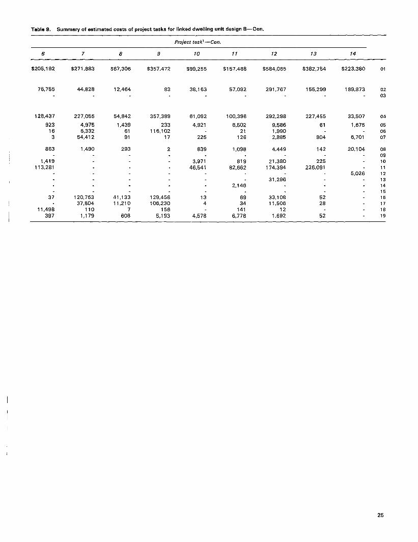
Table 9, Summary of astimatad costs of project taska for linked dwelling unit design B—Con.


6 7 8 9 10 11 12 13 14

$205.192 $271,883 $67,306 $357,472 $99,255 $157,488 $584,065 $382.754 $223,380 01

76,755 44,828 12,464 83 38,163 57,092 291,767 155,299 169,873 0203

128,437 227,055 54,842

1,4396191

357,389 61,092

4,921

225

100,396 292,298 227,455

61

804

33,507 04

050607

92316

3

4,9756,332

54,412

233116,102

17

6,50221

126

9,5861,9902,885

1,67.5

6,701

863

1,419

113,281

1,490 293 2 839

3,97146,541

1,098 4,449 142

225

226,091

5228

52

20,104 080910111213141516171819

81962,662

21,380174,394

5,026

41,13311,210

7608

31,2962,146

37 120,75337,804

1101,179

134

6934141

6,778

33,10811,506

121,692

129,456106,230

156

5,193

11,498397 4,578

25

Table IO. Summa~of estimated coats ofproject tasks forlinked dwelling unit design C

Project taskl


01

02

03

04

05

06

07

08

09

10

11

12

13

14

15

16

17

18

19

Total . . . . . . . . . . . . . . . . . . . . . . . . . . . .


On-site . . . . . . . . . . . . . . . . . . . . . . . . . .

Off-site . . . . . . . . . . . . . . . . . . . . . . . . . .

Other direct cost

Total . . . . . . . . . . . . . . . . . . . . . . . . . . . .

Materials and supplies . . . . . . . . . . . . .Services . . . . . . . . . . . . . . . . . . . . . . . . .Shipping and communications. , . . . . .Travel:

On-site . . . . . . . . . . . . . . . . . . . . . . . .Off-site . . . . . . . . . . . . . . . . . . . . . . . .

Consultants . . . . . . . . . . . . . . . . . . . . . .Computer services . . . . . . . . . . . . . . . . .Reports and reproductions. . . . . . . . . .Interviewer services . . . . . . . . . . . . . . .Interviewer expenses . . . . . . . . . . . . . .Respondent incentives . . . . . . . . . . . . .Clerical labor . . . . . . . . . . . . . . . . . . . . .Clerical labor surcharge . . . . . . . . . . . .Miscellaneous . . . . . . . . . . . . . . . . . . . .Overtime expensea . . . . . . . . . . . . . . . .

.$7,147,752

1,574,037344,486

5,229.229

79,277280,203225,072

56,813357,644

27,914986,252269,012

1,067,987673,587203,245611,365317,242

21,64251.974

$72,697

64,592

8,105

241455440

1,043

2,914544

2,468

$288,961

21,296

267,665

1,1271,134

684

1,986147

261,601

629263

6430

$52.723

13,16421,276

18,281

6581,5824,971

7506,586

12608

2,514

207

67506

$856,020

37,46062,579

755,981

58730,54114,679

14,530286,792

239,148163,797

2,3261,356

1872,038

$2,359,208

298,543260,529

1,800,036

32,79928,796

100,307

8,20164,119

2,134777,819503,687203,245

40,84322,969

1,76213,353

1Legend for project taakx

1 = Survey sampling.8 = Oata coding operations.

9 = Data entry operations.2 = Instrument and materials development. 10= Control card development, mamtenance, and production.3 = Field preparations. 11 = Summary development, maintenance, and production,4 = Survey training. 12= Other data processing operations.5 = Oata collection. 13 = Database construction.

6 = Control system development and production. 14= Project administration.7 = Dsta recaipt, editing, and document control.

26

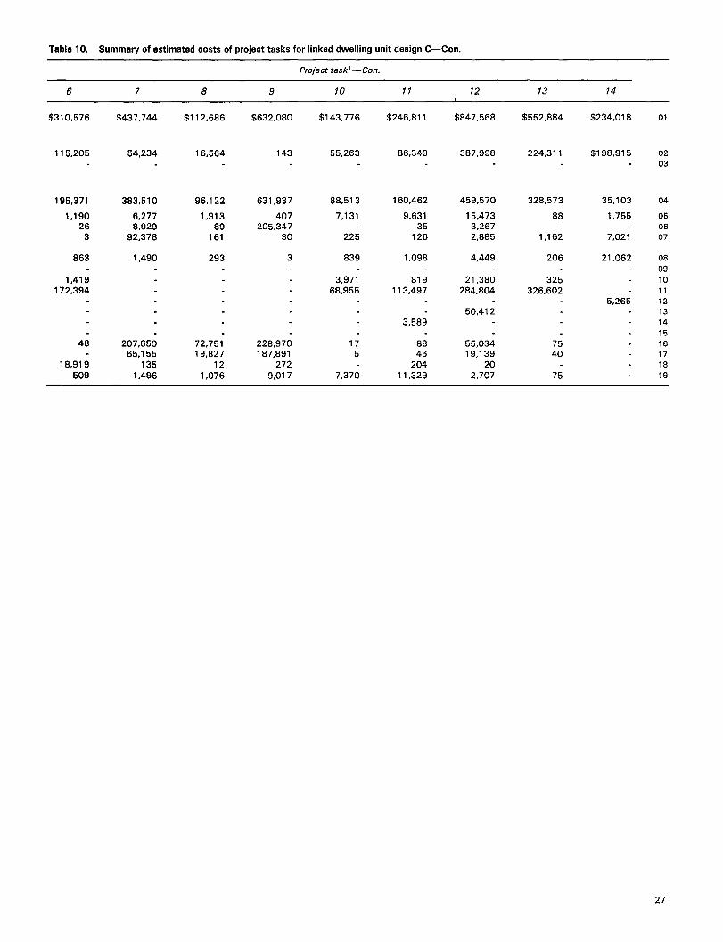
Table 10, Summary of estimeted costs of project tasks for linked dwelling unit design C—Con.

Project task~ —Con.

6 7 8 9 10 11 12 13 74

$310,576 $437,744 $112,686 $632,080 $143,776 $246,811 $847,568 $%!52,884 $234.018 01

115,205 54,234 16,564 143 55,263 86,349 387,998 224,311 $198,915 0203

195,371 383,510

6,2778,929

92,378

96,122

1,81389

161

631,937

407205,347

30

86,513

7,131

160,462 459,570 328,573

88

35,103

1,755

7,021

04

1,19026

3

9,63135126

15,4733,2672,885

050607225 1,162

839

3,97168,955

863 1,490 293 3 1,098 4,449 206

325326,602

21,062 0809

1011121314

15161716

19

1,419172,394

819113,497

21,380284,804

5,26550,412

207,65065,155

1351,496

72,75119,827

121,078

175

7,370

3,589

8846

20411,329

48

18,918509

228,970187,891

2729,017

55,03419,139

202,707

7540

75

27

Table 11. Summary of estimeted costs of project tasks for linked dwelling unit design D

Project taskl


01

02

03

04

05

06

07

08

09

10

11

12

13

14

15

16

17

18

19

Total . . . . . . . . . . . . . . . . . . . . . . . . . . . .

Dmect technical labor

On-sNe . . . . . . . . . . . . . . . . . . . . . . . . . .Off-site . . . . . . . . . . . . . . . . . . . . . . . . . .

Other direct cost

Total . . . . . . . . . . . . . . . . . . . . . . . . . . . .

Materials and supplies . . . . . . . . . . . . .Serwces . . . . . . . . . . . . . . . . . . . . . . . . .

Shlpplng and communications. . . . . . .

Travel:

On-site . . . . . . . . . . . . . . . . . . . . . . . .Off-site . . . . . . . . . . . . . . . . . . . . . . . .

Consultants . . . . . . . . . . . . . . . . . . . . . .

Computer services . . . . . . . . . . . . . . . . .

Reports and reproductions. . . . . . . . . .Interviewer services . . . . . . . . . . . . . . .Interviewer expenses . . . . . . . . . . . . . .Respondent incentives. . . . . . . . . . . . .

Clerical labor . . . . . . . . . . . . . . . . . . . . .

Clerlcal labor surcharge . . . . . . . . . . . .

Miscellaneous . . . . . . . . . . . . . . . . . . . .Overtime expenses . . . . . . . . . . . . . . . .

$6,930,673

1,568,321

395,372

4,966,980

79,954

263,471

233,331

61,649349,105

27,894

918,373

247,0431,006,041

648,487185,781

575,451298,481

20,39451,525

$69,003

61,373

7,630

224428

412

998

2,703

505

2,360

$266,142

21,034

245,108

1,111

1,122

676

1,962145

239,122

618

2606329

$93,672

22,39737,922

33,353

1,1523,163

8,742

1,38211,659

241,217

5,027

40

14118895

$792,966

35,954

60,050

696,962

563

29,288

13,732

13,946265,307

218,676149,776

2,2371,301

1801,956

$2.413.978

338,811

297,400

1,777,767

35,527

30,054

112,162

13,15171,994

2,632739,516490,381

185,781

60,800

28,5321.977

15,270

1Legend for pro]ect tasks 8 = Data coding operations.1 = Survey sampllng. 9 = Data entry operations.2 = Instrument and matenala development. 10= Control card development, maintenance, and production.3 = Field preparauons. 11 = Summary development, maintenance, and production.4 = Survey tralntng. 12 = Other data processing operations,5 = Data collection. 13 = Database construction.6 = Control system development and production. 14 = Project administration.7 = Oata receipt, ednmg, and document control.

28

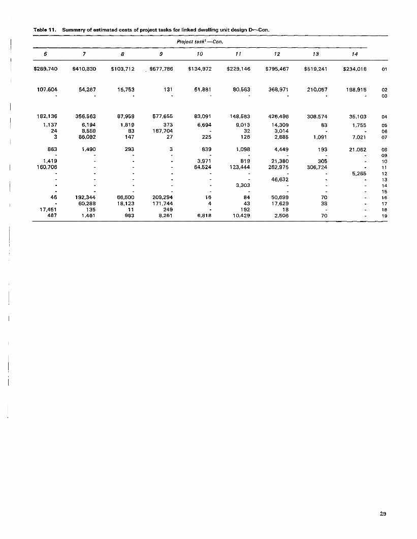
Table 11. Summary of estimated costs of project taaks for linked dwelling unit design D—Con.


6 7 8 9 10 11 12 13 14

$289,740 $410,830 $103,712 $577,786 $134,972 $229,146 $795,467 $519,241 $234,018 01

107,604 64,267 15,753 131 51,881 80,563 368,971 210,057 198,915 0203

182,136 356,!i63 87,959

1,81983

147

577,655

373187,704

27

83,091

6,694

225

148,583 426,496 308,574

83

35,103

1,755

7,021

04

050607

1,13724

3

6,1948,659

86,092

9,01332

126

14,309

3,0142,685 1,091

863 1,490 293 3 839

3,97164,524

1,098

819123,444

4,449 193

305306,724

21,062 06091011

1213141516171819

1,419160,706

21,380262,975

5,26546,632

3,303

46

17,451487

192,34460,288

1351,461

66,50018,123

11983

209,294171,744

2498,261

50,69917,629

182,506

7038

70

164

6,818

8443

19210,429

29

Chapter 4The linked household design

Another approach to linking the National Medical Ex-penditure Survey (NMES) to the National Health InterviewSurvey (NHIS) is to designate as sampling units the NHISsample households rather than the sample addresses. This ap-proach facilitates data collection because sample members areknown in advance. However, some sample members will movebefore round 1 and will have to be located. This approach wasinvestigated using the two primary sampling unit (PSU) sizeoptions and the two precision constraint sets of the originatingbase reporting unit (OBRU) unlinked designs with 6,000 and10,000 responding.

Definition

The linked household design selects NHIS householdsrather than dwelling units. However, the sampling units are theindividual members of these subsampled NHIS households.These individuals are key members of the NMES sample,These key individuals are interviewed in round 1 of NMESwhether or not they live at the same NHIS address, Thus, trac-ing and followup of movers is needed in the first round of datacollection. Because family-level analyses are conducted inNMES, the members of families formed by the sample indi-viduals need to be interviewed. Most households remain thesame in the time period between NHIS and NMES. Becauseindividuals within NHIS households are selected as a group,stable households are entirely composed of NMES key indi-viduals.

Movement into and out of established families is not un-common, however. The guidelines for handling this movementin round 1 are similar to those used in later rounds of NMESunder all design options. That is, individuals who join familiesformed by key individuals through birth or return from the mili-tary, an institution, or overseas residence are included as keyindividuals in NMES. Other individuals joining the families ofkey individuals are classified as nonkey. The distinctionbetween key and nonkey sample members is that only key in-dividuals are included in person-level analyses. Data for nonkeypersons are only used in developing family-level aggregates.Key individuals are followed through all five rounds of datacollection. Nonkey individuals have data collected only for thetime period in which they belong to a family containing a keyindividual.

The frame for the linked household design is a list ofNHIS sample households with names, addresses, and informa-tion needed for tracing, NHIS not-at-home cases are also in-cluded but not NHIS refusals. The frame is strat~led based on

characteristics related to NHIS oversampling to produce a self-weighting sample.

Because the short NHIS data collection period results in alarge percent of nonresponse due to failure to fmd someone athome, excluding these cases would adversely affect the NMESresponse rate. Including these addresses presents a problem,however, because residents present at the time of the NHISinterview may move prior to the NMES round 1 interview andbe replaced by new tenants. The movement problem can behandled by including special screening procedures for NHISnot-at-home cases. However, the problems associated withmovement from NHIS refusals led to their exclusion from theframe for this design.


In a procedure similar to that discussed in the previouschapter, sample sizes were developed for the four designs re-sulting from the two PSU size options and the two sets of vari-ance constraints. First the design variance was modeled, Theintent was not to build an optimal design so only NHIS over-sampling was removed and the design was not stratified priorto selection. Therefore, the variance modeling and sample sizedetermination are the same as those described for the linkeddwelling unit design. However, converting responding OBRU’Sinto the required number of reporting unit interviews is differentfrom the linked dwelling unit design.

Cost modeling

The target population for NMES is the civilian noninstitu-tionalized residents of the United States during the data collec-tion year. Sample individuals are eligible for NMES datacollection only during the time they are civilian, noninstitution-alized, and residing in the United States. Determining the costsfor NMES required modeling the rate at which NHIS indi-viduals leave the NMES target population through death, insti-tutionalization, or emigration, before the NMES data collectionperiod.

Response and attrition rates differ for the linked householddesign. Loss occurs due to movement before NMES as well asattrition effects associated with the previous NHIS interview,Tracing is needed in round 1, and more interviews need to beconducted outside the sample clusters, due to the additionalmovement occurring before round 1.

The first step in the costing process was to model the 1980NMCUES experience. Movement could only be detected forNMCUES when there was a change of ZIP code. First the

30

ZIP codes associated with the original clustered addresseswere determined. In each data collection round, the reportingunits (RU’S) were classified as to whether the interview oc-curred within the ZIP-code-defined clustered areas. Additionalintmiewer travel time and expenses are incurred for interviewsoutside clustered areas. The only interviews occurring outsidethe sample clusters in round 1 were for college students livingaway from home,

When a household moves, there is a one-time only tracingcost to determine the new address. To model this event, a movewas defined as when the ZIP code in a round differs from thatof the previous round. Both movement outside the clusters andtracing are expected to be greater for the linked householddesign,

Table 12 presents the results of this modeling of the 1980NMCUES, Because NMCUES costs occurred to the reportingunit level, these sample sizes are given for RU’S. Because the1980 NMCUES was a clustered area sample of addresses,many of the selectiom were ineligibleunits (vacant, nonresident,and so forth), which accounts for the large number of ineligibleRU’S in round 1, College students living away ftom home re-quire a separate interview and, thus, are assigned a separateRU number. These college students living away from homeaccount for the 92 RU interviews conducted outaide the sampleclusters in round 1. By definition, no tracing was needed inround 1. After round 1, there were costs associated with fol-lowing up sample members who were ineligible or lost to thesurvey population due to death, institutionalization, entranceinto the military, or migration out of the country. There werealso costs associated with attempting interviews with nonre-spondents. In round 2, for instance, 6,727 RU’S were fielded.Of these, 14 were ineligible for the study, 199 failed to respond,and 6,514 completed interviews. Of the 6,514 completing in-terviews, 395 had moved since round 1, requiring tracing andperhaps a reassignment of the RU to another interviewer. The6,514 completed interviews had 6,352 conducted within theZIP code areas associated with the initial sample selectionsand 162 outside these areas. The 395 RU’S requiring tracingmay or may not have moved outside the sample clustered ZIP”codes. After round 2, these cases did not require additionaltracing unless they moved again. However, those of the 395RU’S who moved outside the sample clusters required moreinterviewer traveltime and expenses to complete their inter-views,

The expected sample sizes needed to yield the requirednumber of completed OBRU interviews are given in table 13for the four linked household designs. Assumptions were madein deriving these sample sizes. First, the required number ofresponding OBRU’S were converted into RU costing units byassuming that the ratio of the number of completed interviewsin a round and the number of responding OBRU’S would be thesame for all designs. With this assumption, the number ofcompleted interviews in each round was estimated as the productof the number of responding OBRU’S times each round’s ratioof completed RU interviews to responding OBRU’S.

Because the linked household design will encounter move-ment in round 1, the percent of interviews outside the sampleclusters should be greater than that in round 1 of the unlinked

design. To estimate the extent of the movement, it was assumedthat the linked household design encounters similar movementoutside the clusters in round 1 to that of the unlinked design inround 2; that round 2 movement outside the clusters is simliarto that encountered by the unliiked design in round 3; and soforth. These projected rates were modified to account for lessinterviewing outside the clusters in round 4 when college stu-dents have returned home for the summer. The percent of thecompleted interviews where tracing is required should be similarin the linked and unlinked designs, except for round 1 of theunlinked design, which does not encounter movement. Theround 2 tracing rate for the unlinked design was used to modelthe round 1 tracing rate for the linked household design.

Modeling the response rate was the next step. The cumu-lative responses and attrition rates that the 1980 NMCUESencountered were 91.1 percent in round 1; 90.7 percent in round2; 89.7 percent in round 3; 89.3 percent in round 4; and 89.0percent in round 5. Excluding the 2.5 percent NHIS refusalsfrom the NMES frame allows the liied household survey betterroundwise response rate than that of the unlinked design. Thefact that the sample would have been interviewed once alreadywould have a negative effect. Balancing these two factors, thecumulative attrition and response rate expected in the field is92,5 percent in round 1; 91.5 percent in round 2; 91.1 percentin round 3; 90.8 percent in round 4; and 90.5 percent in round5. An additionrd 2.5 percent of the NMES sample would belost due to NHIS refusal and exclusion from the frame, resultingin effective cumulative response and attrition rates of 90.2,89.2, 88.8, 88.5, and 88.2 percent in rounds 1 through 5, re-spectively.

The rate at which sample members become ineligible wasmodeled in a procedure similar to that of the tracing rate model.That is, it was assumed that in every round after the fwst thepercent ineligible of the total sample fielded is the same for thelinked household design as for the 1980 NMCUES. The round1 ineligible rate for the linked household design was based onthe rate in round 2 of the 1980 NMCUES.

Unit costs were developed by round to include identifyingineligible RU’S, attempting to interview nonrespondlng RU’S,completing interviews within the sample clusters, completinginterviews outside the sample clusters, and tracing movers.These unit costs were used in modeling the costs for the fourlinked household designs. These costs are presented in tables14–17. The 6,000-OBRU-equivalent linked household designhas duect costs of $4,891,831 with 100 PSU’S and $4,967,406with 200 PSU’S, compared with $4,963,013 for the unlinked6,000-OBRU design. The 10,OOO-OBRU-equivalent linkedhousehold design has direct costs of $7,182,341 with 100PSU’S and $6,962,291 with 200 PSU’S, compared with$7,209,409 for the unlinked 1O,OOO-OBRUdesign. These re-sults suggest that 200 PSU’S are more cost efllcient for the1O,OOO-OBRUprecision constraints than 100 PSU’S, but aremore liiely a reflection of instability of the variance constraints.(See chapter 5.)

The cost savings associated with linkage are not substantial.Savings for the design, a slightly larger response rate, and nocounting and listing costs, are partly offset by added costs as-sociated with tracing movers.

31


Between the time of the NHIS interview and the beginningof the NMES data collection year, individuals enter the targetpopulation through birth or through return from the military, aninstitution, or overseas. The unlinked household design updatesthe sample in round 1 using the same procedure as that of allNMES designs. That is, individuals who joined families formedby NMES subsampled individuals enter the survey as key in-dividuals if they were born or returned from an ineligible stateafter the NHIS interview. This procedure results in under-coverage of the individuals entering the target population who

do not join preexisting families. All NMES designs encounterthis type of undercoverage in rounds 2–5 of the study, but onlythe linked household design encounters this in round 1. Thisundercoverage is not substantial enough to preclude the use ofthe linked household design, but the dwelling unit design ispreferable for optimum population coverage.

By restricting attention to self-weighting designs, thus far,many of the advantages associated with the liikage of NMESto NHIS have been eliminated. The next chapter departs nomthe self-weighting constraint to investigate optimal versions ofthe linked household design.

32

Table 12. Sampla sizes for the 1980 National Medical Care Utilization and Expenditure Survey (N MCUES) design

RU’S completing interviews

Reporting Inside Outsideunits (RU’S) RU’S sample

Roundsample

ineligible nonresponding Total Traced clusters clusters

1 .......................................... 1,115 643 6,601 6,509 922 . . . . . . . . . . . . . . . . . . . . . . . . . . . . . . . . . . . . . . . . . . 14 199 6,514 395 6,352 1623 . . . . . . . . . . . . . . . . . . . . . . . . . . . . . . . . . . . . . . . . . . 24 94 6,525 2464

6,355 170. . . . . . . . . . . . . . . . . . 3

5 : : : : : : : : : : : : : : : : : : : : : : ::....... . . . . . . . . . . .72 4,558 114 4,482 76

26 57 6,559 183 6,418 141

Teble 13. Sempla sizes for the Netional Medical Expenditure Survey (N MES) linked household design

RU’S completing interviews

Reporting inside Outsideunits (RU’S) RWS sample sample

Design type and round ineligible nonresponding Total Traced clusters clusters

Design A

Round . . . . . . . . . . . . . . . . . . . . . . . . . . . . . . . . . . . . 14 498 6,165 172 6,012 153Round . . . . . . . . . . . . . . . . . . . . . . . . . . . . . . . . . . . . 23 184 6,084 369 5,925 159Round . . . . . . . . . . . . . . . . . . . . . . . . . . . . . . . . . . . . 23 86 6,094 232 5,935 159Round . . . . . . . . . . . . . . . . . . . . . . . . . . . . . . . . . . . . 3 66 4,257 106 4,186 71Round . . . . . . . . . . . . . . . . . . . . . . . . . . . . . . . . . . . . 24 52 6,126 171 5,981 145

Design B

Round . . . . . . . . . . . . . . . . . . . . . . . . . . . . . . . . . . . . 13 470 5,818 162 5,674 144Round . . . . . . . . . . . . . . . . . . . . . . . . . . . . . . . . . . . . 22 174 5,741 348 5,591 150Round . . . . . . . . . . . . . . . . . . . . . . . . . . . . . . . . . . . . 22 81 5,751 219 5,601 150Round . . . . . . . . . . . . . . . . . . . . . . . . . . . . . . . . . . . . 3 62 4,017 100 3,950 67Round . . . . . . . . . . . . . . . . . . . . . . . . . . . . . . . . . . . . 23 49 5,781 161 5,644 137

Design C

Round I . . . . . . . . . . . . . . . . . . . . . . . . . . . . . . . . . . . . 23 831 10,290 287 10,035 255Round . . . . . . . . . . . . . . . . . . . . . . . . . . . . . . . . . . . . 38 307 10,154 616 9,889 265Round . . . . . . . . . . . . . . . . . . . . . . . . . . . . . . . . . . . . 38 144 10,172 387 9,907 265Round . . . . . . . . . . . . . . . . . . . . . . . . . . . . . . . . . . . . 5 110 7,105 177 6,986 119Round . . . . . . . . . . . . . . . . . . . . . . . . . . . . . . . . . . . . 40 87 10,225 285 9,983 242

Design D

Round . . . . . . . . . . . . . . . . . . . . . . . . . . . . . . . . . . . . 21 760 9,406 262 9,173 233Round . . . . . . . . . . . . . . . . . . . . . . . . . . . . . . . . . . . . 35 281 9,282 563 9,039 243Round . . . . . . . . . . . . . . . . . . . . . . . . . . . . . . . . . . . . 35 131 9,297 354 9,054 243Round . . . . . . . . . . . . . . . . . . . . . . . . . . . . . . . . . . 5 101 6,495 162 6,387 108Raund 5 . . . . . . . . . . . . . . . . . . . . . . . . . . . . . . . . . . . . 37 79 9,346 261 9,125 221

33

Table 14. Summary of astimated costs of project tasks for linkad household design A

Project taskl


01

02

03

04

05

06

07

08

09

10

11

12

13

14

15

16

17

18

19

Total . . . . . . . . . . . . . . . . . . . . . . . . . . . . .


On-site . . . . . . . . . . . . . . . . . . . . . . . . . . . .Off-site, . . . . . . . . . . . . . . . . . . . . . . . . . . .

Other direct cost

Total . . . . . . . . . . . . . . . . . . . . . . . . . . . . .

Materials and supplies. . . . . . . . . . . . . . .Services . . . . . . . . . . . . . . . . . . . . . . . . . . .Shipping and communication . . . . . . . .Travel:

On-site . . . . . . . . . . . . . . . . . . . . . . . . . .Off-site. . . . . . . . . . . . . . . . . . . . . . . . . .

Consultants . . . . . . . . . . . . . . . . . . . . . . . .

Computer services . . . . . . . . . . . . . . . . . .Reports and reproductions. . . . . . . . . . . .Interviewer services . . . . . . . . . . . . . . . . .Interviewer expenses . . . . . . . . . . . . . . . .Respondent incentives. . . . . . . . . . . . . . .Clerical labor. . . . . . . . . . . . . . . . . . . . ,,.Clerical Iebor surcharge . . . . . . . . . . . . . .

Miscellaneous . . . . . . . . . . . . . . . . . . . . . .Overtime expenses . . . . . . . . . . . . . . . . . .

$4,891,831

1,230,862275,026

3,385,943

58,620180,229

161,436

52,738243,404

27,821

669,623163,302662,362424,103121,771

375,848194,613

14,16635,906

$55,462 $182,510 $52,723 $560,811 $1,608,317

49,575 20,076 13,164 30,411 233,01821,278 50,741 203,007

5,887

161327

308

834

1,931361

1,965

162,434

1,051

1,076

645

1,872139

156,734

581248

6028

18,281

6581,582

4,971

7508,586

12608

2,514

207

67506

479,659

47524,673

10,245

11,796186,203

143,303

98,151

1,908

1,098153

1,654

1,172,292

25,11420,981

78,425

8,20150,476

1,530485,671321,180121,771

30,30516,975

1,37410,289

‘Legend for pro]ect tasks: 8 = Data coding operations.1 = Survey sampllng. 9 = Data entry operations.2 = Instrument and materials development. 10 = Control card development, maintenance, and pr~d”~tl~”,3 = Field preparations. 11 = Summary development, maintenance, and producoon.4 = Survey training. 12= Other data processing operations,5 = Data collection. 13 = Database construction.6 = Ccntrcl system development and productmn. 14= Project administration.7 = Data receapt, edltmg, and document control.

34

Tabla 14. Summary of estimated costs of project tasks for linked household design A—Con,

Project task~ —Con.

6 7 8 9 10 11 12 13 14

$213,374 $278,007 $70,829 $378,794 $102,712 $164,423 $604,526 $395,963 $223,380 01

79,741 42,383 12,782 87 39,491 59,363 299,240 160,658 189,873 02

0 03

133,633 234,624 58,047 378,707 63,221 105,060 305,286 235,305 33,507 04

944 4,876 1,476 247 5,092 6,745 10,043 63 1,675 05

16 6,369 63 123,031 22 2,089 063 65,956 96 18 225 126 2,885 832 6,701 07

863 1,490 293 2 839 1,098 4,449 147 20,104 0809

1,419 3,971 819 21,380 232 10

117,871 48,282 86,609 182,966 233,895 115,026 12

32,780 13

2,258 14

38 125s34715

43,688 137,183 13 7039,307 11,879

34,811 53 16

112,571 412,074

35 12,099 29 17107 7 165 146 13 18

405 1,172 645 5,490 4,795 7,132 1,771 54 19

35

Table 15. Summary of estimated costs of project tesks for linked household design B

Project task~


01

02

03

04

05

06

07

08

09

10

111213141516171819

Total . . . . . . . . . . . . . . . . . . . . . . . . . . . .

Direct technical Iebor

On-site. . . . . . . . . . . . . . . . . . . . . . . . . .Off-site . . . . . . . . . . . . . . . . . . . . . . . . . .

Other direct cost

Total . . . . . . . . . . . . . . . . . . . . . . . . . . . .

Materials and supplies . . . . . . . . . . . . .Services . . . . . . . . . . . . . . . . . . . . . . . . .Shipping end communications. . . . . . .

Travel:On-site . . . . . . . . . . . . . . . . . . . . . . . .Off-site . . . . . . . . . . . . . . . . . . . . . . . .

Consultants . . . . . . . . . . . . . . . . . . . . . .Computer services . . . . . . . . . . . . . . . . .Reports and reproductions. . . . . . . . . .Interviewer services . . . . . . . . . . . . . . .Interviewer expenses . . . . . . . . . . . . . .Respondent incentives. . . . . . . . . . . . .Clerical labor. . . . . . . . . . . . . . . . . . . . .

Clerical labor surcharge . . . . . . . . . . . .Miscellaneous . . . . . . . . . . . . . . . . . . . .Overtime expenses . . . . . . . . . . . . . . . .

$4,967,406

1,268,649334,910

3,363,847

61,968176,495177,983

57,969249,388

27,814642,969155,062653,515431,835114,913370,655191,849

13,89237,539

$54,010

46,311

5,699

154316297

816

1,848345

1,923

$173,550

19,974

153,576

1,0451,071

642

1,862138

147,906

577247

6028

$93,672

22,39737,922

33,353

1,1523,1638,742

1,30211,659

241,2175,027

4014

118895

$535,022

29,79649,707

455,519

46524,160

9.857

11,558177,414

134,93192,416

1,8721,076

1501,620

$1,762,357

281,847247,281

1,233,229

28,83723<26393,181

13,15160,177

2,106486,071332,246114,91341,69723,351

1,64012,596

1Legend for project tasks 8 = Data coding operations.1 = Survey sampllng. 8 = Data entry operationa.2 = Instrument and materials development.3 = Field preparations.

10= Control csrd development, maintenance, and productmn.

4 = Survey training.11 = Summary development, maintenance, and production.

5 = Data collection.12= Other data processing operations.13 = Databaae construction.

6 = Control system development and production. 14= Project administration.7 = Data receipt, editing, and dccument ccntrcl.

36

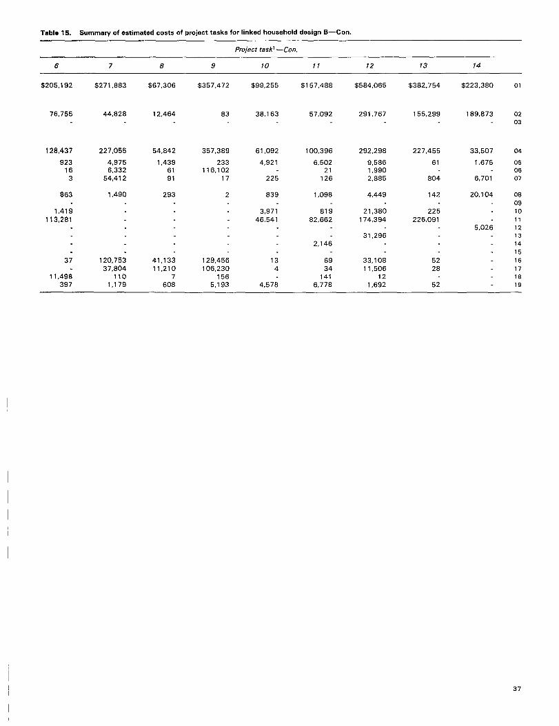
Table 15. Summa~ of estimated costs of project tasks for linked household dasign B—Con.

Project task’ —Con.

6 7 8 9 10 11 12 13 14

$205,192 $271,883 $67,306 $357,472 $99.255 $157,488 $584,065 $382,754 $223,380 01

76,755 44,828 12,464 83 38,163 57,092 291,767 155,299 189,873 0203

128,437 227,055 54,842 357,389 61,092 100,396 292,298

9,5861,9902,885

227,455 33,507

1,675

6.701

04

92316

3

4,9756,332

54.412

1,4396191

233116,102

17

4,921 6,50221

126

61 050607225 804

863

1,419

113,281

1,490 293 2 839 1,098

81982,662

4,449

21,380174,394

31,296

142

225226,091

20,104 0809101112

13

14

15

16

17

18

19

3,97146,541

5,026

2,146

37 41,13311,210

7608

129,456106,230

1565,193

134

4,578

5228

120,75337,804

1101,179

6934

141

6,778

33,10811,506

121,692

11,498397 52

37

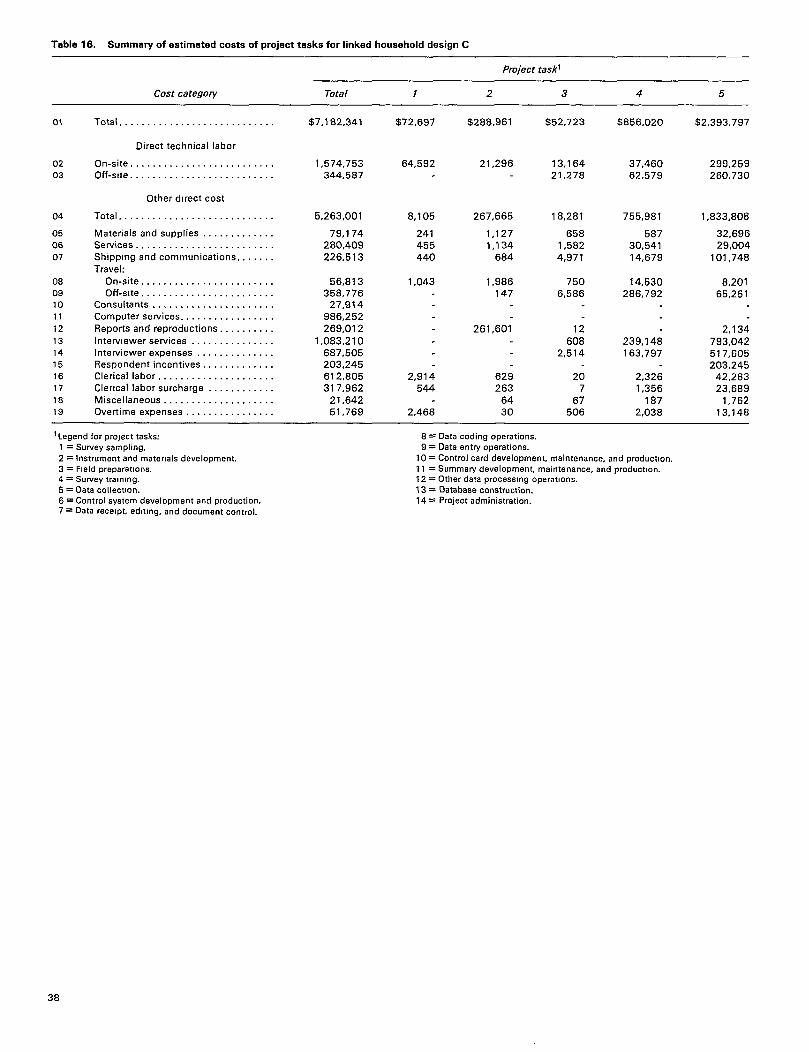
Table 16. Summa~of estimated costaof project tasks forlinked household deaign C

Project taskl


01

02

03

04

05

06

07

08

09

10

11

12

13

14

15

16

17

18

19

Total . . . . . . . . . . . . . . . . . . . . . . . . . . . .


on-site..........................Off-sit e . . . . . . . . . . . . . . . . . . . . . . . . .

Other direct coat

Total . . . . . . . . . . . . . . . . . . . . . . . . . . . .

Materials and supplies . . . . . . . . . . . . .Services . . . . . . . . . . . . . . . . . . . . . . . . .Shipping and communication. . . . . . .Travel:

On-site . . . . . . . . . . . . . . . . . . . . . . . .Off-site . . . . . . . . . . . . . . . . . . . . . . . .

Consultants . . . . . . . . . . . . . . . . . . . . . .Computer services . . . . . . . . . . . . . . . . .Reports and reproductions. . . . ., . . . .

Interwewers ervicea . . . . . . . . . . . . . . .Interviewer expenses . . . . . . . . . . . . . .Respondent incentives. . . . . . . . . . . . .Clerical labor . . . . . . . . . . . . . . . . . . . . .Clerical labor surcharge . . . . . . . . . . . .Miscellaneous . . . . . . . . . . . . . . . . . . . .

Overtime expenses . . . . . . . . . . . . . . . .

$7,182,341

1,574,753344,587

5,263,001

79,174280,409226,513

56,813358,776

27,914966,252269,012

1,083,210687,505203,245612,805317,962

21,64251,769

$72,697

64,592

8,105

241455440

1,043

2,914544

2.468

$288,961

21,296

267,665

1,1271,134

684

1,986147

261,601

629263

6430

S52,723

13,16421,278

18,281

6581,5824,971

7506,586

12

6082,514

207

67506

$856,020

37,46062,579

755,981

58730,54114,679

14,530286,792

239,148163,797

2,3261,356

1872,038

$.2,393,797

299,259260.730

1,833,808

32,69629,004

101,748

8,20165,251

2,134793,042517,605203,245

42,28323,689

1,76213,148

1Legend for project tasks: 8 = Data coding operations.1 = Survey sampling. 9 = Data entry operations.2 = Instrument and materials development. 10= Control card development, maintenance, and production.3 = Field preparations, 11 = Summary development, maintenance, and production.

4 = Survey tralnlng. 12 = Other data processing operations.

5 = Oata collection. 13 = Oatabaae construction.

6 = Control ayatem development and production. 14= Project administration.7 = Oata receipt, edltmg, and document control.

38

Table 16, Summary of estimated costs of projeot taska for linked household design C—Con,


6 7 8 9 10 11 12 13 14

$310,576 $437,744 $112,666 $632,080 $143,776 $246,611 $847,568 $552,884 $234,018 01

115,205 54,234 16,564 143 55,263 86,349 387,998 224,311 $198,915 0203

195,371 363,510 96,122 631,937 88,513 160,462 459,570 328,573 35,103 04

1,190 6,277 1,913 407 7,131 9,631 15,473 88 1,755 0526 8,929 89 205,347 35 3,267 06

3 92,378 161 30 225 126 2,885 1,162 7,021 07

863

1,419172,394

48

18,919509

1,490 293

207,65065,155

1351,498

72,75119,827

121,076

3

228,970187,891

2729,017

839

3,97168,955

175

7,370

1,098

819113,497

3,589

8846

20411,329

4,449

21,380284,804

50,412

55,03419,139

202,707

206

325326,602

7540

75

21,062

5,265

08091011

1213141516171819

39

Table 17. Summa~of estimated costs ofproject teskafor linked housahoIddasign D

Project taskl


01

02

03

04

05

06

07

08

09

10

11

12

13

14

15

16

17

18

19

Total . . . . . . . . . . . . . . . . . . . . . . . . . . . .


On-site . . . . . . . . . . . . . . . . . . . . . . . . . .Off-site . . . . . . . . . . . . . . . . . . . . . . . . . .

Other direct cost

Total . . . . . . . . . . . . . . . . . . . . . . . . . . . .

Materials and supplies . . . . . . . . . . . . .Services . . . . . . . . . . . . . . . . . . . . . . . . .Shipping and communications. . . . . . .Travel:

On-site . . . . . . . . . . . . . . . . . . . . . . ,,Off-site. . . . . . . . . . . . . . . . . . . . . . . .

Consultants . . . . . . . . . . . . . . . . . . . . . .Computer services . . . . . . . . . . . . . . . . .Reports and reproductions . . . . . . . . . .Interviewer services . . . . . . . . . . . . . . .Interwewerexpenses . . . . . . . . . . . . . .

Respondent incentives . . . . . . . . . . . . .Clerical labor . . . . . . . . . . . . . . . . . . . . .Clerical labor surcharge . . . . . . . . . . . .Miscellaneous . . . . . . . . . . . . . . . . . . . .Overtime expenses . . . . . . . . . . . . . . . .

$6,962,291

1,568,976395,464

4,997,851

79,859263,659234,648

61,649350,140

27,894918,373247,043

1,019,956

661,210185,781576,768299,140

20.39451,337

$69,003

61,373

7,630

224428412

998

2,703505

2,360

$266,142

21,034

245,108

1,1111,122

676

1,962

145

239,122

618260

6329

$93,672

22,397

37,922

33,353

1,1523,1638,742

1,30211,659

241,2175,027

4014

118895

$792,966

35,954

60,050

696,962

56329,28813,732

13,946

265,307

218,676149,776

2,2371,301

1801,956

$2,445,596

339,466297,492

1,808<638

35,432

30,242113,469

13,151

73,029

2,632753,431503,104185,781

52,11729,191

1,97715,082

1Legend for prolect tasks

1 = Suwey sampllng.8 = Data coding operations.

9 = Data entry operationa.2 = Instrument and materials development.

3 = Field preparations.10 = Control card development, maintenance, and production,

4 = Survey training.11 = Summary development, maintenance, and production.

5 = Data collection.12 = Other data processing operations.

13 = Database construction.6 = Control system development and production. 14= Project administration.7 = Data receipt, editing, and doc”mant contro\,

40

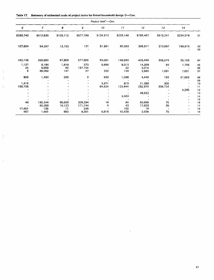
Tabla 17. Summary of estimated costs of project tasks for linked housahold design D—Con.

Project task’ —Con.

6 7 8 9 10 11 12 13 14

S289,740 $410,830 $103,712 $577,786 .$134,972 $229,146 $795,467 $519,241 $234,018 01

107,604 54,267 15,753 131 51,881 80,563 368,971 210,667 198,915 0203

182,136 356,563

6,1948,559

86,092

87,959 577,655

373187,704

27

83,091

6,694

148,583 426,496 308,574

83

35,103

1,755

7.021

04

1,13724

3

1,81983

147

9,01332

126

14,3093,0142,885

050607225 1,091

863 1,490 293 3 839

3,97164,524

1,098 4,449 193

305306,724

21,062 08091011

1213141516171819

1,419160,706

819123,444

21,380262,975

5,26546,632

192,34460,288

1351,461

209,294171,744

2498,261

164

6,818

3,303

46

17,451487

66,50018,123

11983

8443

19210,429

50,69917,629

182,506

7038

70

41

Chapter 5An optimally allocateddesign

Thedesigns previously described areself-weighting andselected by aggregating the National Health interview Survey(NHIS) sample over a short time period. Cost savings resultfrom linkingthese designs to NHIS, but they are not substantial.One reason for the lack of substantial cost savings is that thesedesigns include little of the available NHIS information. Usingthe characteristics of NHIS respondents, greater savings arepossible by stratification and optimal allocation of the sample.

To investigate this, five optimally allocated linked house-hold designs were studied. Two designs are optimally allocatedself-weighting designs, one with the precision of the 6,000originatingbase reporting unit (OBRU) unlinked design, the otherwith the precision of the 1O,OOO-OBRUdesign. Next, the self-weighting constraint was removed for two optimally allocateddesigns, one using the 6,000-OBRU constraints, the secondusing the 1O,OOO-OBRUconstraints. Because increasing thesample size to 10,000 OBRU’S improves precision for smallerdomains such as medicaid recipients, a fifth design was devel-oped using the 6,000-OBRU constraints for the total populationand the 10,000-OBRU constraints for the medicaid subpopu-lation.

Definition

Stratification of the sample is usually proportional tostratum size, except when oversampling of certain populationsubgroups is specified. However, because data collection costsand variances differ among strata, optimal allocation of thesample may result in substantial cost savings. For the NationalMedical Expenditure Survey (NMES), a multipurpose surveywith many outcome measures and reporting domains, the pre-ferred optimization strategy is one that minimizes total surveycost subject to multiple variance constraints. Separate varianceconstraints are set to control the precision of key survey sta-tistics for the total population and for important reportingdomains.

To optimally allocate the sample among strata, cost andvariance models are needed. The following linear function isused to model survey costs for a sample design with L sample

size levels, M(1):

L

c= co+ ~ C(l)tn(l)1=1

(14)

where C = total survey cost

CO= fixed administrative cost of the survey

C(l) = cost of surveying a unit from the lth design levelwhere 1may index a combination of design stages,phases, and strata

m(l) = sample size for the MI design level

The corresponding variance model for a particular statistic anddomain k is

L v’(l)v’=~m

where Vk ==variance of the domain k statistic

V,(l) = variance component associated

(15)

with the kth.. . .domain and s&pling from the kh design level

These cost and variance models illustrate that as the samplesize for each stratum increases, the variance decreases as thetotal cost of the survey increases.

To determine the optimum sample sizes for the L designlevels, the maximum variances (V:) allowed for the designateddomain k estimates must be specified. This maybe representedmathematically as the set of level-spec~lc sample sizes m(l)that minimize the total survey cost C subject to V~S ~ andm(l) 20 for all 1.For a single variance constraint problem, theoptimal allocation to level 1is

[1v(l) 1’2L [v(l)/c(l)]l/2m(l) = —

c(1) z v(16)

1=1

With optimum allocation, these level-specific sampling ratestend to increase as the associated variance increases or thedata collection cost decreases.

Few surveys are conducted to obtain a single estimate.For sample allocation based on the single variance constraintsolution, several estimates would be considered and the designwould be optimized for only one, The preferred strategy simul-taneously considers several estimates chosen by classifying thesurvey statistics according to their variance properties andselecting a typical variance model from each class, Unlike thesingle constraint case, optimization for multiple variance con-

42

straints does not have a closed form solutiow Cochran(pp.119-123)3 reviews a number of approaches to obtain solu-tions for these problems.

The NMES optimization was obtained using an optimiza-tion approach developed by Chromy, described in reference 4.Chromy’s optimization algorithm is an iterative approach thatprovides an optimal solution when the convergence criteria aremet.

NHIS household sampling units provide usefkl informationfor NMES. This information is generally person-level such asage, race, sex, relationship to head of household, limitation ofactivity, bed disability days, perceived health status, medicalconditions, education level, marital status, and employment.Because NMES samples entire households to facilitate family-level analysis, these data must be aggregated to the householdlevel for stratification.

Stratification of the NHIS sample before selection of theNMES sample provides control over the distribution of thesample while increasing the precision of survey estimates. Thevariance of estimates is reduced and the precision increased bysampling stratified to maximize the between-stratum variationand minimize the within-stratum variation. Variables used forstratification should result in homogeneity of the units withinstrata and heterogeneity between strata.

Time constraints prevented the examination of 1980 Na-tional Medical Care Utilization and Expenditure Survey(NMCUES) data to determine which variables should be usedfor stratification of the NHIS sample before NMES sampleselection. Instead, variables that are considered good predictorsof health care utilization and expenditures were used for strat-ification. These variables are black and all other races, agedand not aged, poor and not poor, and self-perceived healthstatus (healthy and not healthy). Sample size limitations of the1980 NMCUES database used to estimate variance com-ponents required collapsing of the black strata over the povertyvariable, resulting in eight all-other-race strata and four blackstrata,

To demonstrate the advantages of an optimum allocationapproach, five optimal designs were developed. The domainsthat were included in the optimization are the total populationand medicaid recipients. For use in stratification, dichotomousOBRU-level variables denoted race (black versus nonblack),poverty status (more or less than 150 percent of the oflicialpoverty index), age status (containing no person greater than orequal to 65 years versus containing at least one), and healthstatus (containing no person with poor or fair health versuscontaining at least one). The optimization was conducted fornine utilization and expenditure rates and for the subpopulationwith large out-of-pocket expenses. First, variance modeling fora stratified, linked household design drawn from the first phaseNHIS sample was conducted. Second, the cost component foreach second phase stratum and each stage of the first phaseNHIS design was modeled. Finally, optimization was con-ducted and its results assessed. The optirrdzation programcomputes the total survey costs for the optimal design based onthe unit costs. Because the total cost was available, full scalecosting to evaluate the design was not necessary. Therefore,this step was eliinated for all the optimally allocated designs.

Variance modeling

Using a stratified sampling approach, NMES would esti-mate the mean for domain k as

H

P~(NMES) = ~tik(h)~k(h)h=l

(17)

where ~~(h) = NMES estimated mean for stratum h

tik(h) = NHIS-estimated fraction of the kth subpopula-tion total person-years associated with the hthstratum

H = number of sample strata

For the nine utilization and expenditure measures, thestratum mean is estimated as

where W(i) = sampling weight of the ith person

6Ji) = 1 if the ith person belongs to the kth domain andOif not

Y(i) = response of the ith person

T(i) = fraction of the year that the ith person was eli-gible for NMES

For the proportion burdened with large out-of-pocket expenses,the stratum mean is estimated as

~FV(i)r3,(i)T(i)Y(i)

Yk(h) = ‘eh~ W(i)tlk(i)T(i)

(19)

iEh

where Y(i) = 1 if the annualized out-of-pocket expenses arelarge (more than $200) and O if not.

To simplfi modeling the variance, it is assumed that NHISoversampling of black persons is at the last stage and that blackand all other races is a stratification variable. Therefore, thevariance of the stratified estimate is modeled as

var [~k(NMES)] = Var~~ls {EIYk(NIIW)

+ ‘NHIS{V=[~JNWl)

‘VaI’NH1~[~&NHIS)]

H Il;(h)s;(h)[l –m)]+ ENHl~z

h=l m(h)

43

H 7r;(h)~(h)[l –fill)]+x (~o)

h=l E[m(h)]

where Dw(k) = design effect for NHIS unequal weighting forthe kth domain

~(PSU) = between NHIS primary sampling unit (PSU)variance component for domain k

~(SEG) = between NHIS segment, within NHIS PSUvariance component for domain k

~(OBRU) = between NHIS OBRU, within NHIS segmentvariance component for domain k

~(h) = stratum h variance for domain k

fib) = NMES subsampling rate for stratum h or m(h)/n(h)

m(h) = NMES stratum h OBRU sample size

n(h) = NHIS stratum h OBRU sample size

The variance components computed from the 1980 NMCUESwere used to estimate the NHIS components. A Taylor seriesapproximation for the simple random sampling variance of acombined ratio estimator was used to estimate fi(h).

The expected NMES sample size from the hth stratumcan be expressed as

E[wz(h)] = ri~h)n’(h) (21)

where i(h) = expected fraction of the NHIS sample from the

hth strata or

Jcf(h)o(h)d(h) = ~

~Af(h)o(h)h=l

(22)

and M(h) is the population count of OBRU’S in stratum h.Assuming that black and all other races is used as a strati-

fication variable with equal probability sampling within strata,the design effect for unequal weighting in domain k estimationis modeled as

(23)

where rr~ = proportion of black persons in the population

mAoR= proportion of all other races in the population

19~= proportion of black persons in the NHIS sample

0*OR = proportion of all other races in the NHIS sample

Because

and

‘AORe

‘OR = 1.41rB+ 7rAoR

Dw(k) may also be expressed as

O.16nB7rAoRDW(k)=l+ 14

.

(24)

(25)

(26)

For convenience, relative variance components are usedin the optimization. To model the relative variances,

Var [~’(NMES)]RVk(NMES) =

~(NMES)(27)

For domain k, the relative variance of a mean estimated usingthe linked household design can be expressed as

where 1= 1, 2,. ... H are the second phase strata used inselecting the NMES subsample, and H 4- 1 and H + 2 are thefirst phase segment and PSU sampling stages.

Cost modeling

If C(l) represents the variable unit cost for a selection fromlevel 1,then the optimization problem maybe stated as follows:Minimize

H- I-2

CV(NMES) = ~ nz(l)C(l)1=1

subject to

H+2Rvk(l)1“~ m(l)

—~RV~fork =1,2, . . ..K

2. m(l) ZOforl=l,2, . . ..H+2

3. 200S m(H+2)< m(H+ 1)

4. m(l)< m(H+l)for l=l,2,.. .,H

where CV(NMES) = total variable cost for NMES

R ~ = relative variance constraint fordomain

(29)

the kth

44

The wwiablecosts for the PSU stage of sampling [C(IZ + 2)]and the segment level of sampling [C(H + 1)] were obtainedby aggregating the task-level unit costs determined by the costmodeling of the self-weighting linked household design costmodeling (chapter 4). The unit costs for the subsampledOBRU’S within NHIS-defined strata vary depending on theresponse and movement rates within the strata. In a proceduresimilar to that described in chapter 4 for the total population,the 1980 NMCUES experience was used to estimate the ratesat which ineligibles, nonrespondents, and movers are en-countered and to develop the OBRU-level cost component foreach of the 12 strata. The unit costs developed for the self-weighting linked household design for tracing movers, inter-viewing ineligibles, and interviewing outside and inside theclusters were used in formingthe total unit costs for each stratum.

Optimization results

The first design investigated is a stratified, self-weightinglinked household design, Using this design, the variance is ex-pressed as in equation (20) wherej(h) =~\o(h). The factor~isthe subsampling rate desired for the NMES subsample ofNHIS after NHIS oversarnpling is removed. The Chromy op-timization procedure was used to obtain optimum values forthe number of PSU’S, the average number of segments tosample per PSU, and the NMES subsampling rate used withinthe sample segments (~ ~ andfl. For use in the optimization,the simplified variance function is recast in the form of equation(15) as

[%(~)u;(pwlVar [~.(NMES)] =

+

—

+

r

DW(k)cr:(SEG) + DW(k)a:(OBRU)/Z

K

&fi(h)S:(h)/n’(h)7h=]

rF

~m;(h)s;(h)~(h)/ti’(h)h=l

(30)r~f

Correspondingly recasting the linear cost model leads to Hsecond phase stratum cost parameters of the form

(31)

The optimization was performed twice. When the varianceconstraints associated with the 6,000-OBRU unlinked designwere used, the optimal solution was 102 PSU’S, 1,258 segments,and 5,980 responding OBRU’S. Wh.h a subsampliig rate ~ of83 percent, black strata are subsampled at a 59-percent rate

Wl .4) ~d all-other-race strata at the 83-percent rate. Thetotal cost for the desi~ is $4,844,013 compared with $4,963,013for the unlinked design with the same precision.

When the variance constraints associated with the 10,000-OBRU unlinked design are used, the optimal stratified linkedhousehold design has 103 PSU’S, 2,117 segments, 9,960 re-sponding OBRU’S, and a subsampling rate ~ of 82 percent.Allowing for the NMES oversampling, black strata are sub-sampled at a 58-percent rate and all-other-race strata at the 82-percent rate. The total cost for this design is $6,931,233 com-pared with $7,209,409 for the unlinked design with the sameprecision.

The stratified household design, with 1O,OOO-OBRUpre-cision, incorporates 103 PSU’S. The unstratified design, pre-viously described in chapter 3, is most cost efficient with 200PSU’S. This difference is the result of instability of the estimatedvariance components used to obtain the sample sizes for theunstratified designs.

The next set of designs investigated are the stratified linkedhousehold designs without the self-weighting constraint. Theadvantage of this type of design is that heavy utilizers of healthcare services can be identified and oversampled. For use in theoptimization, the variance given in equation (20) was recastfollowing equation (15 ).

Dw(k)cr~(Psu)Var[~k(NMES)] =

r

, DW(k)u;(SEG) + DW(k)~(OBRU)/T+

~ m;(h) S~(h)/t#(h)+~ (32)

h=l rif(h)

To optimize over PSU’S (r), segments (r~), and NMES strata(h=l,2,..., If), the stratified linked sample has H + 2 de-sign levels. Using expression (32) for the variance, revised unitcosts are computed for each of the H second phase strata or

c’(/) = C(l)fn’(1) (33)

The total population and medicaid recipients are used inthe optimization. Medicare recipients, the poor, and those infamilies with college educated heads of households were notincluded because an instability of the variance componentswas observed with negative segment-level variance componentsfor some domain estimates. Due to time constraints, examina-tion and correction of the negative components were not possible.

First, an optimally allocated design with the precisionconstraints of the unlinked 6,000-OBRU design for the totaland medicaid domains was investigated. The optimal solution

45

used 98 PSU’S, 1,152 segments, and 5,880 respondingOBRU’S with subsampling rates ranging from 57– 100 percent.In general, the not healthy and all-other-race groups aresampled at a higher rate than is the black group. Greater per-cents of NHIS all other race persons are selected than blackpersons because the number of black persons occurs at a rate1.4 times greater than that for persons of all other races in theNHIS sample. The total cost for this design is $4,770,353compared with $4,963,013 for the unlinked 6,000-OBRU de-sign and $4,844,013 for the self-weighting optimally allocateddesign.

Next, an optimrdly allocated design with the precision ofthe 1O,OOO-OBRUunlinked design for the total and the med-icaid domains was investigated. The optimal solution used 106PSU’S, 1,811 segments, and 9,717 responding OBRU’S withsubsampling rates ranging from 59–100 percent. The total costfor the design is $6,758,063 compared with $7,209,409 for the1O,OOO-OBRUunlinked design and $6,931,233 for the opti-mally allocated self-weighting design.

For household samples drawn from area frames, there islittle information available for use in sample stratification, Toobtain the required sample sizes for small domains, a samplesize larger than usual is frequently used. With household-levelstratification information, these small domains can be over-sarnpled without increasing the size of the total sample.

To illustrate this advantage, an optimally allocated design,with the precision of the unlinked 10,000-OBRU design for themedicaid domain and of the 6,000-OBRU design for total pop-ulation estimates, was developed. These constraints result inan optimal design with 95 PSU’S, 2,092 segments, and 7,228responding OBRU’S with NMES subsampling rates rangingfrom 32-100 percent. The total cost for the design with 6,000and 10,000 OBRU’S is $5,601,533, which compares well withthe $6,758,063 cost for the comparable not-self-weighting de-sign with 10,000-OBRU constraints for both the total andmedicaid domain statistics. Tables 18-20 summarize the re-sults of these comparisons.


NMES will have many small analysis domains includingthe medicaid, the medicare, the aged, the poor, and the blackpopulations. In the past, separate analyses have been madepossible by selecting self-weighting samples large enough toobtain adequate precision for these domains. This approachresults in precision greater than necessary for large domainssuch as the not-aged or white domains. Without linkage, how-ever, this is the best approach because household characteristicsare not available for use in sampling,

Although beyond the scope of this report, precision con-straints for the NMES should be set for a large group of policy-relevant domains. With linkage to NHIS, there is much infor-mation about households that can be used to create an optimallyaJlocated design with increased precision for selected domains.The stability of the variance components and the accuracy ofthe cost components should also be considered, Finally, costmodeling should include the effect of the aggregation length ofthe NHIS sample.

The reporting domains to be included in the optimizationneed carefid attention. Precision is assured for statistics anddomains included in the optimization, The precision for otherstatistics and domains will depend on their relation to the sta-tistics and domains included in the optimization.

The optimizations were designed for total utilization andexpenditure statistics for the total population and for the med-icaid population. The stratiiled self-weighting linked householddesign insures precision for these domains and statistics byselecting a self-weighting design with a sufficient sample size.In the stratified linked household designs without the self-weighting constraint, the precision for these statistics wasmaintained and the cost decreased by oversampling the poorand the not healthy and undersampling the not poor and thehealthy. For domains and statistics not included in the optimi-zation, neither of these optimal designs may yield statistics ofthe desired precision.

Examples from the optimization described in this chapterdemonstrate this point. The stratified self-weighting linked de-sign, optimized for the variance constraints of the 6,000-OBRUunlinked design, may not produce estimates of the desired pre-cision for small domains such as newborns. Using the varianceconstraints for the 1O,OOO-OBRUunlinked design, the samplesize for newborns still may not be sufficient to support detailedanalyses. Increasing the sample size of the self-weightingdesignyields increased precision for such small domains and greaterprecision than necessary for large domains.

Without the self-weighting constraint, an optimally allo-cated design can be created that obtains the desired precisionfor a small domain by oversampling ffom strata where domainmembers are concentrated. If the 10,000-OBRU unlinked de-sign yields the required variance constraints for the medicaiddomain, the self-weighting linked design to use is that whichyields the variance constraints of the 1O,OOO-OBRUunlinkeddesign for all domains. If the 6,000-OBRU unlinked designyields variance constraints acceptable for the total population,the not-self-weighting optimally allocated linked design canachieve both sets of variance constraints by oversamplingstrata with a high concentration of medicaid recipients. Thesurvey costs with the not-self-weighting approach (the not-self-weighting design with 6,000 total and 10,000 medicaidprecision constraints in table 19 are $5,601,533 compared with

$6,931,233 for the self-weighting design (the self-weightingdesign with 10,000 and 10,000 respondents in table 19).

The disadvantage of the optimally allocated not-self-weighting approach is that it may not yield estimates of thedesired precision for domains and statistics not included in theoptimization. The not-self-weighting design with 6,000 totaland 10,000 medicaid precision constraints produces estimatesof the desired precision for the total utilization and total ex-penditure statistics by oversarnpliig from the not healthy strata,If total income is being estimated instead, estimates of the de-sired precision can not be assured because the design does notcontrol for the precision of income estimates. Alternatively, iftotal utilization or total expenditures are being estimated fora domain not included in the optimization, such as the medicaredomain, the design may not yield estimates of the desired pre-cision. The precision of estimates for domains and statistics

46

not included in the optimization depends on their relation tothe statistics and domains included in the optimization.

Although most surveys include many domains and sta-tistics, this does not preclude use of a not-self-weighting optimally allocated design, A strategy using this design is to con-sider several estimates chosen by classi&ing their varianceproperties and splecting a typical variance model from eachclass,”Similarly, the domains to include in the optimization canbe chosen by listing the important domains and selecting thosethat represent diverse groups of the population.

Because extreme groups are usually rare, they must berepresented in the set of domains subject to optimization toobtain an adequate sample size. For example, a survey com-paring health expenditures for different income groups should

include the poor and the wealthy as domains in the optimization.It may not be necessary to include the large middle incomeportion of the population as a domain, particularly if the totalpopulation is included as a domain in the optimization.

Linkage of NMES to NHIS makes available the names,addresses, and personal characteristics of sample householdsbefore data collection. The design with the most potential forusing this information is the stratii3ed not-self-weighting op-timally allocated design. Research to produce this design woulddetermine the domains and statistics of interest to the surveyand the appropriate set to include in the optimization. The1980 NMCUES data could be used in constructing varianceand cost models. The advantages of implementing an optimallyallocated design should far exceed the costs of its development.

47

Table 18. Sample sizes for the alternata optimally allocated dasigna

Originating

base

Primary reporting

sampling unitsDesign type units Segments (OBRU’S) cost

Self-weighting, precision of6,0000BRU design . . . . . . . . . . . . . . . . . . . . . . . . . . . . . . . . . . . . 102 1,258 5,980 $4,844,013Self-waighting, precision ofl0,000 OBRU design . . . . . . . . . . . . . . . . . . . . . . . . . . . . . . . . . . . 103 2,117 9,960 6,931,233Not-self-weighting, precieion of 6,000 OBRU design. . . . . . . . . . . . . . . . . . . . . . . . . . . . . . . . . 98 1,152 5,880 4,770,353Not-self-weighting, precision of 10,000 OBRU design . . . . . . . . . . . . . . . . . . . . . . . . . . . . . . . 106 1,811 9$717 6,758,063Not-self-weighting, precision of 6,000 total OBRU and 10,000 madicaid OBRU designs ., . 95 2,092 7,228 5,601,533

Table 19. Stratum sampling ratas for tha altarnate optimally allocatad dasigne

Design type

Notself- weighting,

precision ofNot Not 6,000 total

Self-weighting, Self-weighting, self- weighting, self- weighting, OBRU andprecison of precision of precision of precision of 70,000

6,000 OBRU 10,000 OBRU 6,000 OBRU ?0, 000 OBRU medicaidStrata dasign design design design OBRU designs

All other races, not aged, not poor, healthy. . . . . . . . . . .

All other races, not aged, not poor, not healthy . . . . . . .

All other races, not aged, poor, healthy. , . . . . . . . . . . . .

All other races, not aged, poor, not healthy. . . . . . . . . . .All other races, aged, not poor, healthy. . . . . . . . . . . . . .All other races, aged, not poor, not healthy. . . . . . . . . . .All other races, aged, poor, healthy . . . . . . . . . . . . . . . . .All other races, aged, poor, not healthy. . . . . . . . . . . . . .Black, notaged, healthy . . . . . . . . . . . . . . . . . . . . . . . . . .81ack, notaged, not healthy . . . . . . . . . . . . . . . . . . . . . . .81ack, aged, heaIthy . . . . . . . . . . . . . . . . . . . . . . . . . . . . . .

81ack, aged, not healthy . . . . . . . . . . . . . . . . . . . . . . . . . .

83

83

838383838383

59595959

8282

828282828282

585858

58

8699

76100

83100

8887

617657

100

9499

79

10084

1009777

677959

100

4195

63100

32937272

597635

100

OBRU = originating baae reporting unit.

Table 20. Stratum originating base reporting unit (08RU) sampla sizes for the alternate optimally allocatad designs

Design type

Notself- weighting,

precision of

Not Not 6,000 total

Self-weighting, Self-weighting, self- weighting, self- weighting, OBRU and

precison of precision of precision of precision of 10,000

6,000 OBRU 10,000 OBRU 6,000 OBRU 10,000 OBRU

Strata

medicaiddasign design design design OBRU designs

All strata . . . . . . . . . . . . . . . . . . . . . . . . . . . . . . . . . . . . . . . 5,980 9,960 5,880 9,717 7,228All other racea, not aged, not poor, healthy. . . . . . . . . . . 2,826 4,707 2,697 4,622 2,328All other races, not aged, not poor, not healthy . . . . . . . 556 927 612 957 1,069All other races, not aged, poor, healthy. . . . . . . . . . . . . . 451 751 380 625 574All other races, not aged, poor, not healthy. ., . . . . . . . . 250 416 277 435 503

All other races, aged, not poor, healthy. . . . . . . . . . . . . . 461 768 422 674 298All other races, aged, not poor, not healthy. . . . . . . . . . . 279 464 309 486 524All other races, aged, poor, healthy . . . . . . . . . . . . . . . . . 268 446 262 454 390

All other races, aged, poor, not healthy. . . . . . . . . . . . . . 265 441 256 356 38381ack, notaged, healthy, ,,, . . . . . . . . . . . . . . . . . . . . . . 351 585 332 573 586Black, notaged, not healthy . . . . . . . . . . . . . . . . . . . . . . . 152 254 179 293 328Black, aged, healthy . . . . . . . . . . . . . . . . . . . . . . . . . . . . . . 52 87 47 75 5281ack, aged, not healthy, ,. . . . . . . . . . . . . . . . . . . . . . . . 69 114 107 167 193

OBRU = ongmating base reporting unit.

48

I

Chapter 6Comparison of the designsand recommendations

The National Medical Expenditure Survey (NMES) designtypes investigated in this study have similar features. Regardlessof how the sample is selected, all of the designs assume thateach sample household is interviewed personally in rounds 1,2, and 5, and that the telephone is used whenever possible inrounds 3 and 4.

Each design defines key persons to be followed for allrounds of data collection. The designs also define key personsas those who, in rounds 2-5, are either born or return from themilitary, overseas, or a long-term care institution and enter anexisting family, All other persons who are members of familiesformed by key persons are classified as nonkey. Nonkey per-sons have data collected for them only as long as they belong tofamilies with members who are key persons. The data for keypersons are used for person-level analyses; nonkey person dataare only used to construct aggregated data used in family-levelanalyses.

In round 1, a household roster is obtained, and health caredata are collected for all household members including collegestudents living away from home. During the first interview, thehousehold is given a calendar diary and instructed as to its use,Art incentive of $5 is paid to the household and its membersare advised that another $5 will be paid to them at the end ofthe survey. The household is advised that a summary of thereported health care data will be mailed to its members beforeeach interview so that erroneous or missing information can becorrected.

Round 2 is also conducted by personal interview for thedesign types investigated in this study. The advantages of asecond personal interview round are that the interviewer canreview the summary with the responden~ and, because the bulkof survey attrition occurs at round 2, a personal interview shouldreduce the level of attrition early in the survey and commit therespondent to the survey.

The next two rounds of data collection use the telephonewhenever possible. Because round 4 is at the end of the year,not all respondents are included. Because December 31 is theend of the survey reference period, approximately 30 percentof the sample is not interviewed in round 4 but, instead, early inround 5 (that is, shortly after January 1 of the next year).

The fifth and final round of data collection is conducted bypersonal interview. In addition to obtaining the health caredata through December 31 of the past year, the round 5 inter-view obtains annual income and other data that are not availableuntil aiter the end of the reference period.

The same target population definition is used by the Na-

tional Health Interview Survey (NHIS) and NMES, whichfacilitates using the NHIS sample as a frame for NMES. Bothsurveys define their target populations as the civilian noninsti-tutionalized residents of the United States. NHIS is based on anational area sample of housing units and group quarters and issimilar to the 1980 National Medical Care Utilization andExpenditure Survey (NMCUES) design except for the sam-pling of college students. NHIS includes college students in thesample when their college residence is sampled. Because of itsinterest in family-level analyses, NMES links college studentswho are single, 17–22 years of age, and living away from hometo their parents’ residence. Only when the parents’ residence isselected is the college student included in the sample. The dif-ference between the definitions does not present problems forlinkage of NMES to NHIS provided that NHIS identifies allcollege students who are single, 17–22 years of age, and livingaway from home and asks sample NHIS families to providename and address information for these college students.

Four types of sample designs were investigated in thisstudy, including two unlinked designs, four linked NHIS andNMES dwelling unit designs, four linked NHIS and NMEShousehold designs, and five optimally allocated linked house-hold designs. Table 21 summarizes the sample size and costfor the 1980 NMCUES and for the 14 designs investigated foruse in the 1987 NMES. The cost of the five optimally allocateddesigns compares well with that of the other designs. Thesecosts were constructed from the 1980 NMCUES experienceand are not adjusted for inflation.

Table 21 includes the months that the NHIS sample mustbe aggregated to obtain the required number of sample segmentsfrom the specified number of primary sampling units (PSU’S).These estimates of aggregation time are based on the assump-tions that NHIS includes 8,750 segments and 200 PSU’S foran average of 43.75 segments per PSU in a year and thatNMES is selected from the 90 percent consisting of personalinterviews. The aggregation times range from 1.5–6.7 months;the longer periods of aggregation are required for the optimallyallocated designs. Modeling of movement is only approximate,so the costs associated with movement may be understated,particularly for designs that aggregate over a longer period oftime. More attention needs to be given to cost modeling ofmovement as the time between NHIS and NMES increases.

In modeling the costs for the designs it is assumed that theNMES contractor selects the sample. The NHIS interviewerin the NMES-subsampled segments is given a three-put tear-sheet on which to record the information needed in the NMES

49

sample selection. This information includes names and ad-dresses, NHIS-identifiers, andperson characteristics neededfor stratification. The tearsheet is completed at the time ofNHIS data collection. The tearsheeta are distributed on a flowbasis, one copy to the contractor, one copy to the U.S. Bureauof the Census field office, and one copy to the interviewer’srecords. With this approach, the contractor constructs the frameon a flow basis. The Census field oftice also reviews the docu-ments on a flow basis and advises the contractor of any dis-crepancies. With the tearsheet approach, the NMES samplecan also be selected by the U.S. Bureau of the Census or theNational Center for Health Statistics.

For costing the sampling effort, it is assumed that the con-tractor does the frame construction and sampling. An advantageof selection by the contractor is quality control. NME S is acomplex study that requires integration of the effort of samplingstatisticians, survey operations specialists, and computer pro-grammers. To coordinate NMES activities and ensure thequality of the product, the contractor should have direct controlover all project activities.

The cost savings demonstrated by the optimally allocateddesigns, particularly the not-self-weighting designs, indicatethat there are signfiicant savings possible with NHIS linkage.Further study would be needed to construct such a design forNMES. It is recommended that a full scale design study beconducted before the 1987 NMES to determine the samplesize parameters of the design. This study should identfi pmtential high expenditure respondents from NHIS data and usethis information to improve the precision of survey estimates toreduce the data collection costs for the survey.

Proposed NMES design parameters should be tested in apilot study before implementation. This pilot study should testlinkage methods, data collection alternatives, and questionnairechanges since the 1980 NMCUES. The use of NHIS-derivedinformation should be considered as a means to reduce the data

collection costs of NMES. In this investigation the data col-lection pattern of the 1980 NMCUES was followed. However,this approach may not be necessary when an NHIS-based listfkame is available.

It appears possible that one or more of the personal inter-view rounds could be replaced by a telephone interview roundwithout adversely affecting response rates. The first roundshould use personal interviews whenever possible. Personalcontact is necessmy to establish the creditability of the study,to persuade the respondent to participate, and to instruct therespondent in the use of the calendar diary and the summary.Telephone numbers available from NHIS may be used tomake appointments, reducing data collection costs. Before im-plementing this, the procedure should be tested in a pilot studyto determine its impact on response.

Another strategy that could be tested is using NHIS toobtain round 1 data for NMES. Using this approach, NHISfamilies to be included in NMES would have the NHIS in-strument administered along with a supplement to obtain therequired NMES round 1 data not normally obtained by NHIS.For example, NHIS obtains health care expenditures and util-ization data for the week before data collection. The NMESsupplement would collect additional data for the period sinceJanuary 1. If this combined NHIS and NMES interview appreach were effective, one round of data collection could beeliminated. If this strategy is considered for NMES, a pilotstudy should be conducted to determine whether adding aNMES supplement to selected NHIS family interviews wouldcontaminate either NHIS or NMES data. This question ofNHIS contamination could be tested by comparing NHIS datacollected in the usual manner with NHIS data collected when aNMES supplement was used. The question of the effect onNMES could be tested by comparing NMES data obtained byNHIS interviewers with an NMES supplement with NMESdata obtained in an independent NMES interview.

50

Table 21. Sampla size summary for the alternete National Medical Expenditure Survey (NM ES) design

Sample size

Originating

Primary base reporting

sampling units

DesignAggregation Direct

untts Segments [OBRU’S] time cost

Unlinked designs

6,000 -respondent OBRU’s .,..... . . . . . . . . . . . . . . . . . . . . . . . . . . . . . .10,000 .respondent OBRU’s . . . . . . . . . . . . . . . . . . . . . . . . . . . . . . . . . . . . . .

Linked dwelling unit designs

Design A(6,000-respondent OBRU’s) . . . . . . . . . . . . . . . . . . . . . . . . . . . . . .Des!gn B(6,000-respondent OBRU’s) . . . . . . . . . . . . . . . . . . . . . . . . . . . . .

Design C(lO,OOO-respondent OBRU’s) . . . . . . . . . . . . . . . . . . . . . . . . . . . . .Design D(lO,OOO-respondent OBRU’s). . . . . . . . . . . . . . . . . . . . . . . . . . . . .

Linked household designs

Design A(6,000-respondent OBRU’s), . . . . . . . . . . . . . . . . . . . . . . . . . . . . .Design B(6,000-respondent OBRU’s) . . . . . . . . . . . . . . . . . . . . . . . . . . . . . .Design C(lO,OOO.respondent OBRU’s) . . . . . . . . . . . . . . . . . . . . . . . . . . . . .Design D(lO,OOO-respondent OBRU’s). . . . . . . . . . . . . . . . . . . . . . . . . . . . .

Linked stratlfted optimally allocated household designs

Self-weighting, pracision of 6,000 OBRU design. . . . . . . . . . , . . . . . . . . .

Self-weighting, precision of 10,000 OBRU design, . . . . . . . . . . . . . . . . . . .Not-self-weighting, precision of 6,000 OBRU design . . . . . . . . . . . . . . . . .Not-self-wsighting, pracision of 10,000 OBRU design . . . . . . . . . . . . . . . .Not+elf-weighting, precision of 6,000 total OBRU and 10,000 medicaid

OBRUdeslgns . . . . . . . . . . . . . . . . . . . . . . . . . . . . . . . . . . . . . . . . . . . . . . . .

102102

100200100200

100200100200

102

10398

106

95

7501,250

976921

1,6291.4B9

976921

1,6291,489

1,2582,1171,1521,811

2,092

6,00010.000

5,6565,5269,774B,934

5,8565,526987748,934

5,9B09,9605,8809,717

7,228

. . .

. . .

3.01.45.02.3

3.01.45.02.3

3.86.33.65.2

6.7

$4,963,0137,209,409

4,871,1064,947,8487,147,7526,930,673

4,891,8314,967,4067,182,3417,209,409

4,844,0136,931,2334,770,3536,758,063

5,601,533

51

References

1B. V. Shalx VMCPNLS: Program To Compute Variance Com-ponents. Research Triangle Institute. In-house report, 1979.

2G. B. Gray Component of variance model in multi-stage stratitiedsamples. Survey Methodology :27-43, 1975.

3W. G. Cochran: Sampling Techniques. New York. John Wiley andSons, 1977.

4NationaI Center for Health Statistics: R. E. Folsom, Jr., R L. Wil-liams, and J. R Chromy Optimum Design of a Medical Care Ex-penditwe and Utilization Survey Involving a Provider Record CheckReport No. 1725/01-06S. Research Triangle Park, N.C. ResearchTriangle Institute, 1980. .

52

AppendixDescriptionof costmodeling process

This appendix describes the steps required to perform thevarious cost modeling steps completed for the alternative de-signs, Examples provided in tables I-XII for this discussionare for the survey sampling operations task.

Table

I

N

111

IV

Description of activity

Step 1. Research Triangle Institute monthly cost ex-perience for each of the direct cost budget categorieswas abstracted from accounting records during the lifeof the project. The project activity spanned the periodOctober 1979 through the fall of 1981.Step 2. Using the monthly breakdown of projectspending, monthly costs were collapsed to correspondto presurvey setup activity, rounds 1–5, and post-survey wrapup activity periods of time.Step 3. Professional stail, providing the 1980 NationalMedical Care Utilization and Expenditure Surveyproject with fiscal leadership, reviewed the round-by-round cost experience to determine the level of ex-penditures to be associated with fixed and variablecost units of primary sampling units, segments, andreporting units (RU’S). Table III shows the percentsused to distribute the costs over the fixed and variablecategories.Step 4. Once percent allocations were determined,these percents were applied to the actual dollars ex-pended for each of the budget cost categories. TableIV shows actual dollar allocations for the fixed andvariable modeling categories.

v

VI

VII

VIII

IX

x

XI

XII

Step 5. Using various combinations of numbers ex-pected for completed RU’S, numbers of primary sam-pling units, and numbers of segments, the estimatedcosts of alternative designs were generated. Table Vpresents the estimated direct costs to have had onlyResearch Triangle Institute conduct the 1980 Na-tional Medicrd Care Utilization and ExpenditureSurvey design.Procedure designed in step 5 was repeated for the6,000-OBRU design.Procedure described in step 5 was repeated for the1O,OOO-OBRUdesign.Step 6. In preparation for modeling the linked house-hold unweighed design, staff reviewed the fixed andvariable percent allocations used in the modeling todetermine whether any refinements were to be madebased on operational differences of the designs. Theallocation rates for f~ed and variable cost componentswere generated. Presented in table VIII are the dollarallocations for the fried and variable cost categories.Step 7. Using the information prepared during step 6,staff generated the estimated costs to perform activitiesfor the linked household unweighed design A.Procedure described in step 7 was repeated for designB.Procedure described in step 7 was repeated for designc.Procedure described in step 7 was repeated for designD.

53

Tabla 1. Summary of Resaarch Triangle Institute (RTI) cost expariance for survay sampling for the National Medical Care Utilization and

Expenditure Suwey Household Suwey, by month

1979 1980

Prior

3

Cost category Total months Jan. Feb. Mar. Apr.

01

0203

04

050607

08091011

12

13141516171819

Total . . . . . . . . . . . . . . . . . . . . . . . . . . . . . . . . . . . . . . . . . . . . . . . . . . . . . . . . . . . . . . .

Diract technical labor

On-site . . . . . . . . . . .Off-site ynl:lnl jnYIIl:l Unj:n Hn: Y1ll J::: Y:ll:Y1: JI1::I:::: l... . . . . . . . .

Other direct cost

Total . . . . . . . . . . . . . . . . . . . . . . . . . . . . . . . . . . . . . . . . . . . . . . . . . . . . . . . . . . . . . . .

Materials and supplies . . . . . . . . . . . . . . . . . . . . . . . . . . . . . . . . . . . . . . . . . . . . . . . .Sewices . . . . . . . . . . . . . . . . . . . . . . . . . . . . . . . . . . . . . . . . . . . . . . . . . . . . . . . . . . . .

Shipping and communications . . . . . . . . . . . . . . . . . . . . . . . . . . . . . . . . . . . . . . . . . .

Travel:On-site . . . . . . . . . . . . . . . . . . . . . . . . . . . . . . . . . . . . . . . . . . . . . . . . . . . . . . . . . . .Off-site . . . . . . . . . . . . . . . . . . . . . . . . . . . . . . . . . . . . . . . . . . . . . . . . . . . . . . . . . . .

Consultants . . . . . . . . . . . . . . . . . . . . . . . . . . . . . . . . . . . . . . . . . . . . . . . . . . . . . . . . .Computer sewices . . . . . . . . . . . . . . . . . . . . . . . . . . . . . . . . . . . . . . . . . . . . . . . . . . . .Reports and reproductions . . . . . . . . . . . . . . . . . . . . . . . . . . . . . . . . . . . . . . . . . . . . .Interviewer services . . . . . . . . . . . . . . . . . . . . . . . . . . . . . . . . . . . . . . . . . . . . . . . . . .Interviewer expenses . . . . . . . . . . . . . . . . . . . . . . . . . . . . . . . . . . . . . . . . . . . . . . . . .Respondent incentives . . . . . . . . . . . . . . . . . . . . . . . . . . . . . . . . . . . . . . . . . . . . . . . .Clerical labor . . . . . . . . . . . . . . . . . . . . . . . . . . . . . . . . . . . . . . . . . . . . . . . . . . . . . . . .Clerical labor surcharge . . . . . . . . . . . . . . . . . . . . . . . . . . . . . . . . . . . . . . . . . . . . . . .Miscellaneous . . . . . . . . . . . . . . . . . . . . . . . . . . . . . . . . . . . . . . . . . . . . . . . . . . . . . . .Overtime expenses . . . . . . . . . . . . . . . . . . . . . . . . . . . . . . . . . . . . . . . . . . . . . . . . . . .

. . .

$41,138

3,152

98228213

690

3012

1,620

.,.

$7.086

387

4448

295

. . .

$637

55

55

,..

$663

77

467

24

. . .

$245

18

18

. . .

$304

81

81

NOTES: National Household Survey portion = 1.00; RTI portion= 1.00. Number of primary sampling units= 59; number of segments = 404.

Round Round Round Round RoundItem 1 2 3 4 5

Completed parsonal

Intetvews . . . . . . . . . . . . . 3,322 3,293 558 279 3,306Completed telephone

intetwewa. . . . . . . . . . . . . 2,722 2,047

Table 1. Summary of Research Triangle Institute (RTI) cost experianca for survey sampling for the National Medical Cara Utilization andExpenditure Survey Household Survey, by month—Con,

1980—Con. 1981

May June

Other

July Aug. Sept. Oct. Nov. Dec. Jan. Feb. Mar. ARr. Mav months

,..

$50

50

. . .

$666

10

10

.,,

$130

168

168

,..

$290

15

15

. . .

$1,645

. . . . . .

$2,158

. . .

$3,055

58

18

40

. . .

$239

168

30

138

. . .

$564

01

0203

04

05

06

07

08

09

10

11

12

13

14

15

16

17

18

19

.

$1,404

8

8

. . .

$621

311

311

. . . . . .

$1,358 $3,999 $16,074

6 31 1,709

6 6415

31 2

6

2

1,620

Table Il. Summary of Research Triangle lnstituta (RTl)cost experience forsumey sampling forthe National Medical Cara Utilization andExpandlture Survey Household Survey, rounds 1–5

Setup WrapupCost category Total activity Round 1 Round 2 Round 3 Round 4 Round 5 activity

—

Total . . . . . . . . . . . . . . . . . . . . . . . . . . . . . . . . . . . . . . . . . . . . . . . . . . . . . . . . . . . . . .

Dlrecttechnlcal labor

On-site .,. . . . . . . . . . . . . . . . . . . . . . . . . . . . . . . . . .otf-wl?,, . . . . . . . . . . . . . . . . . . . . . . . . . . . . . . . . . . . . .

$41,138 $6,732 $1,899 $970 $3,423 $5,213 $6,827 $16,074

Other direct costs

Total . . . . . . . . . . . . . . . . . . . . . . . . . . . . . . . . . . . . . . . . . 3,152

98228

213

368

4246

0

169

486442

141 189 58 518

830

0

1,709

M.+twmls andsupplles . . . . . . . . . . . . . . . . . . . . . . . . . .%rwces. . . . . . . . . . . . . . . . . . . . . . . . . . . . . . . . . . . . . .

Shlppmg and communications. . . . . . . . . . . . . . . . . . . .Tr.ivel:

On-sNe . . . . . . . . . . . . . . . . . . . . . . . . . . . . . . . . . . . . .Off-sltc . . . . . . . . . . . . . . . . . . . . . . . . . . . . . . . . . . . . .

Consultants . . . . . . . . . . . . . . . . . . . . . . . . . . . . . . . . . . .

Computer serwces. . . . . . . . . . . . . . . . . . . . . . . . . . . . . .Reports .indreproductlons, ..,.. . . . . . . . . . . . . . . . . .Intkrvlswers ervlces . . . . . . . . . . . . . . . . . . . . . . . . . . . . .Interviewer expenses . . . . . . . . . . . . . . . . . . . . . . . . . . . .Respondent incentives .,...... . . . . . . . . . . . . . . . . . .Clerical l~bor . . . . . . . . . . . . . . . . . . . . . . . . . . . . . . . . . .

Ckwcallaborsur charge . . . . . . . . . . . . . . . . . . . . . . . . . .

Mwcelltin@ous . . . . . . . . . . . . . . . . . . . . . . . . . . . . . . . . .Ov@lmee xpenses . . . . . . . . . . . . . . . . . . . . . . . . . . . . .

615

6415

18

0141

690 168 40 480 2

301

2

1,620

280 62

15

1,620

NOTE: Seo note to table 1.

55

Table I Il. Summary of Reseerch Triangle Institute cost experience in percent for survey sampIing for the National Medical Care Utilizationand Expenditure Survay Household Suwey, rounds 1-5

Round 1 Round 2

Fixed Psu Segment RU Fixed Psu Segment RU

Cost cetego~ cost cost cost cost cost cost cost cost

Percent’

. . . . . .Total . . . . . . . . . . . . . . . . . . . . . . . . . . . . . . . .01

02

03

04

. . . . . . . . . . . . . . . . . .


On-site . . . . . . . . . . . . . . . . . . . . . . . . . . . . . .Off-site . . . . . . . . . . . . . . . . . . . . . . . . . . . . . .

40 . . .. . . . . .

30. . .

30 50. . . . . .

50. . .

. . .

. . .. . .. . .

Other direct costs

Total . . . . . . . . . . . . . . . . . . . . . . . . . . . . . . . . . . . . . . . . . . . . . . . . . .

Materials and supplies . . . . . . . . . . . . . . . . .Services . . . . . . . . . . . . . . . . . . . . . . . . . . . . .Shipping and communications. . . . . . . . . . .Trevel:

On-site. . . . . . . . . . . . . . . . . . . . . . . . . . . .

Off-site. . . . . . . . . . . . . . . . . . . . . . . . . . . .Conaultenta . . . . . . . . . . . . . . . . . . . . . . . . . .Computer servicea . . . . . . . . . . . . . . . . . . . . .Reporta end reproductions. . . . . . . . . . . . . .Interviewer aervices . . . . . . . . . . . . . . . . . . .

Interviewer expensea . . . . . . . . . . . . . . . . . .Respondent incentives . . . . . . . . . . . . . . . . .Clerical labor . . . . . . . . . . . . . . . . . . . . . . . . .Clerical labor surcharge ., . . . . . , . . . . . . . .Miscellaneous . . . . . . . . . . . . . . . . . . . . . . . .Overtime expenses . . . . . . . . . . . . . . . . . . . .

40 ,..40 . . .40 . . .

303030

303030

05 . . . . . .. . ..,.

. . .

. . .

. . .

. . .06

“50.,.5007

08

0910111213141516171819

. . .

. . .

. . .

. . .

. . .

. . .

. . .

. . .

. . .

. . .

. . .

. . .

. . .

. . .

. . .

. . .

. . .

. . .

. . .

. . .

. . .

. . .

. . .

. . .

. . .

. . .

. . .

. . .

. . .

. . .

. . .

. . .

. . .

. . .,,.. . .

.,.

. . .

. . .

. . .

. . .

. . .

. . .

. . .

. . .

. . .,... . .

. . .

. . .

. . .

. . .

. . .

. . .

. . .

. . .

. . .

. . .

. . .

. . .

. . .

. . .

. . .,... . .,.,,,.. . .. . .. . .. . .. . .

. . .

. . .

. . .

. . .

. . .

. . .. . .

40......... .

. . .

30.........

,..

30...,.....

1Percents used to allocate fixed and per unit variable costs.

NOTE: PSU = prima~ sampling unit: RU = reporting unit,

Tabla II 1. Summary of Research Triangla Institute cost expariance in parcant for survay sampling for tha National Madical Cara Utilizationand Expenditure Survey Household Survay, rounda 1-5—Con.

Round 3 Round 4 Round 5

Fixed Psu Segment RU Fixed Psu Segment RU Fixed Psu Segment RUcost cost cost cost cost cost cost cost cost cost cost cost

Percentl

. . . 01

02

. . . . . . . . . . . . . . . . . . . . . . . . . . . . . . . . .

75,..

25.,.

85,..

15. . .

75. . .

25. . .

. . .,,.

. . .,..

. . .

. . .. . .. . .

. . .

. . .. . .. . . 03

04. . . . . . . . . .,. . . . . . . . . . . . . . . . . . . . . . . . .

252525

75

7575

05,.,7575

.,.

. . .

. . .

,... . .. . .

!..

2525

. . .85

. . .

. . .

.,.

. . .

. . .

. . .“1”5

. . .

. . .

. . .

. . .

. . .

. . .0607. . . . . .

75 25 85 15 75. . .

. . .

. . .

. . .

. . .

25. . .

. . .

. . .

08. . .,.,,... . .. . ..,.. . .. . .,,.. . .. . .. . .

. . .

. . .

. . .

. . .

. . .,... . .. . .,,.. . .. . .. . .. . .. . .. . .

. . .

. . .

. . .

. . .

. . .

. . .

. . .

. . .

. . .

. . .

. . .,..

. . .

. . .

. . .

. . .

. . .

.,.

. . .

. . .

. . .

. . .

. . .

. . .

. . .

. . .

. . .

. . .

. . .

. . .

. . .

. . .

. . .

. . .

.,.

. . .

09

10111213141516171819

. . .

. . .

. . .

. . .,,.. . .. . .,... . .. . ..,.

.,.

. . .

. . .

. . .

. . .

. . .

. . ..!.

. . .

. . .

. . .

. . .. . .. . .. . .. . .. . .. . .. . .. . .. . .. . .

. . .

. . .

.,,

. . .

. . .

.,,

. . .

. . .

.,.

. . .

. . .

.,.

. . .

. . .

. . .

. . .

. . .

. . .

. . .

. . .

2525. . .. . .

. . .

“7575,..

. . . .,. . . . . . .

57

Tabla IV. Summary of Raaaarch Triangla Inatituta cost experience for survey sampling for the National Medical Care Utilization and ExpenditureSurvay Houaahold Survey, rounds 1-5, by typa of cost

Round 1 Round 2

Fixed Psu Segment RU Fixed Psu Segment RU

Cost category cost cost cost cost cost cost cost cost

01

0203

04

050607

08

0910111213141516171819

Total . . . . . . . . . . . . . . . . . . . . . . . . . . . . . . . . . . .$3,667 .20 $6.81 .$0.83 $555.50 $0.17


On-site . . . . . . . . . . . . . . . . . . . . . . . . . . . . . . . . .Off-site . . . . . . . . . . . . . . . . . . . . . . . . . . . . . . . .

3,452.40 6.41 0.78 485.00 0.15

Other direct costs

Total . . . . . . . . . . . . . . . . . . . . . . . . . . . . . . . . . . 214.80

36.0044.0016.80

0.40

0.070.080.03

0.50 70.50 0.02

Materials andaupplies . . . . . . . . . . . . . . . . . . . .Services. . . . . . . . . . . . . . . . . . . . . . . . . . . . . . . .Shipping and communications . . . . . . . . . . . . .Travel:

On-site . . . . . . . . . . . . . . . . . . . . . . . . . . . . . . .

Off-site . . . . . . . . . . . . . . . . . . . . . . . . . . . . . .Consultants . . . . . . . . . . . . . . . . . . . . . . . . . . . . .Computer sewicea . . . . . . . . . . . . . . . . . . . . . . .Reports and reproductions. . . . . . . . . . . . . . . . .Interviewer services . . . . . . . . . . . . . . . . . . . . . .Interviewer expenaes . . . . . . . . . . . . . . . . . . . . .Respondent incentives . . . . . . . . . . . . . . . . . . . .Clerical labor . . . . . . . . . . . . . . . . . . . . . . . . . . . .Clerical labor surcharge . . . . . . . . . . . . . . . . . . .Miscellaneous . . . . . . . . . . . . . . . . . . . . . . . . . . .

Overtime expenaes . . . . . . . . . . . . . . . . . . . . . . .

0.010.01

0.0270.50

118.00 0.22 0.03

NOTES PSU = primary ssmpling unit; RU = reporting unit. Number of primary sampling units= 59; number of segments= 404.

Round1

3,322

100

40

3030

Round Round2 3

Round5

3,306

100

75

25

ItemCompletad personal

Intewfews . . . . . . . . . . . .Completed telephone

Interwews. . . . . . . . . . . .

cost

Total . . . . . . . . . . . . . . . . .

Fixed .,............,..Psu . . . . . . . . . . . . . . . . . .Segment . . . . . . . . . . . . . .Case. . . . . . . . . . . . . . . . . .

4

279

2,047

3,293 558

2,722

Percant

100 100

50 75

50 25

100

85

15

58

Table IV. Summary of Rasaarch Triangle Institute cost experience for suwey sampling for the Nstional Medical Care Utilization and ExpenditureSuway Houaahold Survey, rounds 1-5, by type of cost—Con.


Fixed Psu Segment RU Fixed Psu Segment RU Fixed Psu Segment RUcost cost cost cost cost cost cost cost cost cost cost cost

$2,709.00 - - $0.28 $4,480.35 - - $0.34 $18,846.00 - $1.90 01

0203

04

050607

080910111213141516171819—

2,567.25 - 0.26. .

4,431.05 - 0.34 17,175.75 - 1.73

141,75 - 0.01 49,30 1,670.25 0.17

6.0070.5011.25

. .4.50 -

11,25 -0.0115.30

126.00 0.01 34.00 361.50 0.04

4.501.50

1,215.00

. .

. .0.12

59

Table V. Summary of estimeted costs for survey sampling with the Research Triangle Institute design componant of tha 1980 NMCUES

Round 1 Round 2

Seg- Seg-Fixed PSU ment RIJ Fixed PSU ment RU

Cost category Total Total cost cost cost cost Total cost cost cost cost

01

02

03

04

05

06

07

08

09

10

11

12

13

14

15

16

17

18

19

Total. . . . . . . . . . . . . . . . . . . . . . . . .


On-site . . . . . . . . . . . . . . . . . . . . . . .Off-site. . . . . . . . . . . . . . . . . . . . . . .

Other direct costs

Total . . . . . . . . . . . . . . . . . . . . . . . . .

Materiala and supplies . . . . . . . . . .Services . . . . . . . . . . . . . . . . . . . . . .Shipping and communications . . .Travel:

On-site. c. . . . . . . . . . . . . . . . . . .

Off-site . . . . . . . . . . . . . . . . . . . . .Consultants . . . . . . . . . . . . . . . . . . .Computer servicea . . . . . . . . . . . . .Reports and reproductions. . . . . . .interviewer aarvices . . . . . . . . . . . .Interviewer expenaea . . . . . . . . . . .Respondent incentives. . . . . . . . . .Clerical labor . . . . . . . . . . . . . . . . . .Clerical labor surcharge . . . . . . . . .Miscellaneous . . . . . . . . . . . . . . . . .Overtime expenses . . . . . . . . . . . . .

$58,147

54,001

4,154

154322322

857

4793

2,019

$14,642

13,784

858

144176

67

471

$3,667

3,452

215

364417

118

$5,508

5,185

323

546625

177

$5,467

5,147

320

546625

176

$1,656

1,445

219

219

$556

485

71

71

$1,100

960

140

140

NOTES Number of prima~ sampling units (PSU’a) = 108; number of segments = 808; RU = reporting unit. Data are based on NMCUES fixed and per un!t allocatlona.


Completed personal

Interwewa . . . . . . . . . . . . 6,603 6,519 1,110 547 6,561

Completed telephone

mterwews . . . . . . . . . . . . 5,418 4,012

60

I Table V. Summary of astimated costs for survey sampling with the Research Triangle Institute design component of the 1980 NMCUES—Con.


Seg- Seg- Seg-Fixed PSU ment RIJ Fixed PSU ment RU Fixed PSU ment RU

Total cost cost cost cost Total cost cost cost cost Total cost cost cost cost

I .$4,506 $2,709 - - $1,797 $6,030 $4,480 - - $1,550 $31,313 $18,846 - - $12,467 01

4.270 2,567 - - 1,703 5,964 4,431 - - 1,533 28,538 17,176 - - 11,362 02. . . . . -. 03

236 142 - - 94 66 49 17 2,775

10118

18

1,670

67111

1,105

447

7

04

050607

080910111213141516171819—

816

. .5--11 - -

1537

20 5

210 126 - -. .. .. .. .

. .

. .

12 601 36284 46 34 239

31

804

. .

. .

. .

. .

. .

52

1,2152,019

61

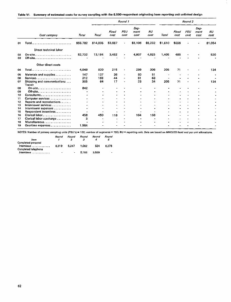
Table W. Summary of estimated costs for survay sampling with the 6,000-respondent originating base raporting unit unlinked design

Round 1 Round 2

Seg- Seg-Fixed Psu ment R.!) Fixed PSU ment W

Cost catego~ Total Total cost cost cost cost Total cost cost cost cost

01

0203

04

05

0607

080910

111213141516171818

Total . . . . . . . . . . . . . . . . . . . . . . . . .

Direct technical Isbor

On-sits . . . . . . . . . . . . .. c....... .Off-site . . . . . . . . . . . . . . . . . . . . . . .

Other direct costs

Total . . . . . . . . . . . . . . . . . . . . . . . . .

Materials and supplies. . . . . . . . . .Services . . . . . . . . . . . . . . . . . . . . . .Shipping and communications . . .Traval:

On-site . . . . . . . . . . . . . . . . . . . . .

Off-site . . . . . . . . . . . . . . . . . . . . .Consultants . . . . . . . . . . . . . . . . . . .

Computer sewices . . . . . . . .. o...Reports and reproductions. . . . . . .Interviewer sarvices . . . . . . . . . . . .Interviewer expenses . . . . . . . . . . .Respondent incentives. . . . . . . . . .Clerical labor . . . . . . . . . . . . . . . . . .

Clericsl labor surcharge . . . . . . . . .Miscellaneous . . . . . . . . . . . . . . . . .Overtime expenses . . . . . . . . . . . . .

$56,782

52,732

4,049

147312305

842

458

3

1,984

$14,005

13,184

820

137168

64

450

$3,667

3,452

215

364417

118

$5,106

4,807

299

506123

164

$5,232

4,925

306

516324

168

$1,610

1,405

205

205

$556

485

71

.

71

.

.

$1,054

920

134

134

NOTES Number of prima~ sampling units (PSU’S) = 102; number of segmsnts = 750; RU = reporting unit. Date are baaed on NMCUES fixed snd per unit allocations.


Completed personalinterviews . . . . . . . . . . . . . 6,319 6,247 1,062 524 6,278

Completed telephoneintewiews . . . . . . . . . . . . . 5,185 3,839

62

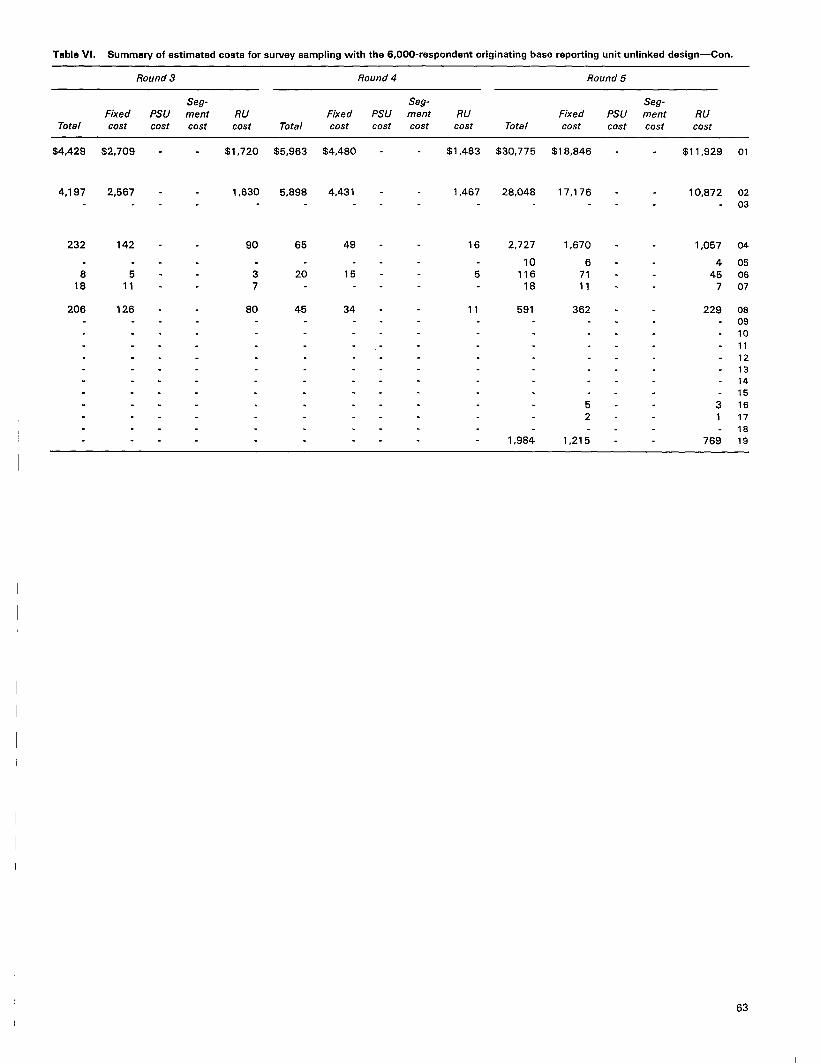
Table V1. Summary of estimated costs for survey sampling with the 6,000-respondent originating base reporting unit unlinked design—Con.


Seg- Seg- Seg-Fixed PSU ment RU Fixed PSU ment RU Fixed PSU ment RU


$4,429 $2,709

2,567

142

511

126

$1,720 $5,963

5,898

65

20

45

$4,480

4,431

49

15

34

$1,483 $30,775

28,048

2,727

10116

18

691

1,984

$18,846

17,176

1,670

67111

362

52

1,215

$11,929 01

0203

04

060607

080910111213141516171819—

4,197 1,630 1,467 10,872

232 90 16 1,057

445

7

818

37

5

206 80 11 229

,-

31

769

63

Table V1l. Summary of estimated costs for survey sampling with the 10,000 -reapondant originating base reporting unit unlinked design

Round 7 Round 2

Seg- Seg-Fixed Psu ment RU Fixed PSU ment RU


01

0203

04

050607

08091011

1213141516

171819

Total, . . . . . . . . . . . . . . . . . . . . . . .

Diract technical labor

On-site . . . . . . . . . . . . . . . . . . . . . . .Off-site . . . . . . . . . . . . . . . . . . . . . . .

Other direct costs

Total . . . . . . . . . . . . . . . . . . . . . . . . .

Msterials and supplias . . . . . . . . . .Services . . . . . . . . . . . . . . . . . . . . . .Shipping and communications . . .Travel:

On-site . . . . . . . . . . ...0.... . . .Off-site . . . . . . . . . . . . . . . . . . . . .

Consultants . . . . . . . . . . . . . . . . . . .Computer setvices . . . . . . . . . . ..cReports and reproductions. . . . . . .Interviewer services . . . . . . . . . . . .Interviewer expenses . . . . . . . . . . .Respondent incentives. . . . . . . . . .Clerical labor . . . . . . . . . . . . . . . . . .

Clerical labor surcharge . . . . . . . . .Miscellaneous . . . . . . . . . . . . . . . . .Overtime expenses . . . . . . . . . . . . .

$74,462

69,142

5,318

218429436

1,055

683

4

2,497

$20,896

19,671

1,224

206251

96

673

$3,667

3,452

215

364417

118

$8,510

8,011

498

84102

39

274

$8,719

8,208

511

86105

40

281

$2,310

2,016

294

294

$556

485

71

71

$1,754

1,531

223

223

.

NOTES Number of primaiy sampling units (PSUS) = 102; number of segments = 1,250; RU = reporting unit. Data sre baaed on NMCUES fixed and per unit allccatlona.


Ccmpletsd personalinterviews . . . . . ...<... 10,531 10,397 1,770 873 10,464

Completed telephone. .Interwewa. . . . . . . . . . . . 8,641 6,398

64

Table WI. Summary of estimated costs for survay sampling with tha 10,OOO-respondent originating baaa reporting unit unlinked design—Con.


Seg- Seg- Seg-Fixed PSU ment RU Fixed PSU ment RU Fixed PSU ment RU


$5,575

5,283

292

1023

259

.

.

.

.

.

$2,709

2,567

142

511

126

. $2,866 $6,952

6,875

76

23

53

$4<480

4,431

49

15

34

$2,472 $38,729

35,297

3,432

12145

23

743

104

2,497

$18,846

17,176

1,670

67111

362

52

1,215

$19,883 01

0203

04

050607

080910111213141516171819—

2,716 2,444 18,121

150 27 1,762

67412

512

8

133 19 381

52

1,282

65

Tabla VIII. Summary of costs for survay sampling for tha linked household dasign

Round 1 Round 2

Fixed Psu Segment RU Fixed PsuCost category

Segment RUcost cost cost cost cost cost cost cost

01

0203

04

050607

080910111213

141516171819

Total . . . . . . . . . . . . . . . . . . . . . . . . . . . . . . . . . . $3,111.20 $5.78 $0.70 $655.50 - $0.17


On-site . . . . . . . . . . . . . . . . . . . . . . . . . . . . . . . . .Off-site . . . . . . . . . . . . . . . . . . . . . . . . . . . . . . . .

2,471 .S0 4.59 0.56 485.00 - 0.15

Other diract costs

Total . . . . . . . . . . . . . . . . . . . . . . . . . . . . . . . . . . 639.60

36.0044.0016.80

1.19

0.070.080.03

0.14 70.50 0.02

Materials and supplies . . . . . . . . . . . . . . . . . . . .Services . . . . . . . . . . . . . . . . . . . . . . . . . . . . . . . .Shipping and communications . . . . . . . . . . . . .

Travel:

On-site . . . . . . . . . . . . . . . . . . . . . . . . . . . . . . .Off-site . . . . . . . . . . . . . . . . . . . . . . . . . . . . . .

Consultants . . . . . . . . . . . . . . . . . . . . . . . . . . . . .Computer services . . . . . . . . . . . . . . . . . . . . . . .Reports and reproductions. , . . . . . . . . . . . . . . .

Interviewer aervices . . . . . . . . . . ..c . . . . . . . . .Interviewer expenses . . . . . . . . . . . . . . . . . . . . .Respondent incentives . . . . . . . . . . . . . . . . . . . .Clerical labor . . . . . . . . . . . . . . . . . . . . . . . . . . . .Clerical labor surcharge . . . . . . . . . . . . . . . . . . .Miacellanaous . . . . . . . . . . . . . . . . . . . . . . . . . . .Overtime expensea . . . . . . . . . . . . . . . . . . . . . . .

0.010.01

70.50 0.02

457.6085.20

0.850.16

0.100.02

NOTES PSU = prima~ sampling unit; RU = reporting unit. Number of primary sampling units= 59; number of segments = 404.


Completed personalinterviews . . . . . . . . . . . . 3,322 3,293 558 279 3,306

Completed telephoneinterviews . . . . . . . . . . . . 2,722 2,047

66

Table WI 1. Summary of coats for survey sampling for the linked household design—Con.


Fixed Psu Segment RU Fixed Psu Segment RU Fixed Psu Segment RU

cost cost cost cost cost cost cost cost cost cost cost cost

$2,709.00 - $0.28 $4,480.35 - $0.34 $18,846.00 - $1.90 01

2,667,25 0.26 4,431.05 0.34 17,175.75 1.73 0203

04141.75 0.01 49.30 1,670.25

6.0070.50

11.25

0.17

0515.30 0.014,50

11.25

126.00

0607

0,01 34.00 361.50 0.04 0809101112

13

14

15

16

17

18

18

.

4.501.50

0.121,215.00.

Table IX. Summary of estimated costs for survey sampling for tha linkad housahold dasign A

Round 1 Round 2



01

0203

04

050607

080910111213141516

171819

Total . . . . . . . . . . . . . . . . . . . . . . . . .


On-site . . . . . . . . . . . . . . . . . . . . . . .Off-site . . . . . . . . . . . . . . . . . . . . . . .

Other direct costs

Total . . . . . . . . . . . . . . . . . . . . . . . . .

Materials and supplies . . . . . i . . . .Services . . . . . . . . . . . . . . . . . . . . . .Shipping and communications . . .Travel:

On-site. . . . . . . . . . . . . . . . . . . . .Off-site. . . . . . . . . . . . . . . . . . . . .

Consultant . . . . . . . . . . . . . . . . . . .Computer sewices . . . . . . . . . . . . .Reporta and reproductions. . . . . . .Interviewer services . . . . . . . . . . . .Intewiewer axpanses . . . . . . . . . . .Respondent incentives. ., . . . . . . .Clerical labor . . . . . . . . . . . . . . . . . .Clerical labor surcharge . . . . . . . . .Miscellaneous . . . . . . . . . . . . . . . . .Overtime expenses . . . . . . . . . . . . .

$55,461

49,575

5,887

161328

307

834

1,932361

1,965

$13,078

10,390

2,689

151185

70

1,924358

$3,111

2,472

640

364417

45885

$5,637

4,478

1,159

658030

829154

$4,330

3,440

890

506123

637119

$1,582

1,381

201

201

$556

485

71

71

$1,026

896

130

130

NOTES Number of primary sampling units (PSU’a) = 100; number of segments = 976; RU = reporting unit.


Complsted personalinterviews . . . . . . . . . . . . . 6,165 6,084 1,036 511 6,126

Completed telephoneinterviews . . . . . . . . . . . . . 5,058 3,746 -

68

Table IX. Summary of estimated costs for survey sampling for the linked household design A—Con.


Seg- Seg- Seg-

Fixed PSU ment RU Fixed PSU ment RU Fixed PSU ment RU

Tote/ cost cost cost cost Total cost cost cost cost Total cost cost cost cost

$4,387 .$2,709

2,587

142

511

126

$1,447 $30,487

27,785

2,702

10115

18

585

1,965

$18,846

17,176

1,670

67111

362

52

1,215

$11,641 01$1,678 $5,927

5,862

85

20

45

$4,480

4,431

49

15

34

4,157 1,431 10,6091,590 0203

230 88 16 1,032

444

7

04

050607

818

37

5

204.

78 11 223 08091011121314

15

16

17

18

19

31

750

69

Table X. Summary of aatirnated costs for survey sampling for the linked household design B

Round 1 Round 2

Seg- Seg-Fixed Psu ment RU Fixed PSLJ ment RU


01

02

03

04

05

06

07

08

09

10

11

12

13

14

15

16

17

18

19

Total . . . . . . . . . . . . . . . . . . . . . . . . . .

Oirect technical labor

On-site . . . . . . . . . . . . . . . . . . . . . . . .

Off-site, . . . . . . . . . . . . . . . . . . . . . . .

Other direct costs

ToteI . . . . . . . . . . . . . . . . . . . . . . . . . .

Materials and supplies. . . . . . . . . . . .

Sewices . . . . . . . . . . . . . . . . . . . . . . .Shipping and communications . . . . .Trevel:

On-site . . . . . . . . . . . . . . . . . . . . . .Off-site . . . . . . . . . . . . . . . . . . . . . .

Consultants . . . . . . . . . . . . . . . . . . . . .Computer servicas . . . . . . . . . . . . . . .Reports snd reproductions . . . . . . . .Interviewer services. . . . . . . . . . . . . .

Interviewer expenses. , . . . . . . . . . . .

Respondent incentives . . . . . . . . . . .Clerical labor . . . . . . . . . . . . . . . . . . .Clerical labor surcharge. . . . . . . . . . .Miscellaneous . . . . . . . . . . . . . . . . . .Overtima expenses . . . . . . . . . . . . . .

$54,009

48,310

5,701

154

317298

817

1,849346

1,923

$12,517

9,944

2,574

145

17768

1,841343

$3,111

2,472

640

36

4417

45B85

$5,319

4,226

1,094

62

7529

782146

$4,087

3,246

840

47

5822

601112

$1,524

1,331

194

194

. ..

5556

485

71

71

.

$988

846

123

123

NOTES: Number of prima~ sampling units (PSU’S) = 200; number of segments = 921; RU = reporting unm.


Completed personal. .mtetwews. . . . . . . . . . . . . 5,818 6,741 978 482 5,781

Complated telephoneinterviews . . . . . . . . . . . . . 4,773 3,535

70

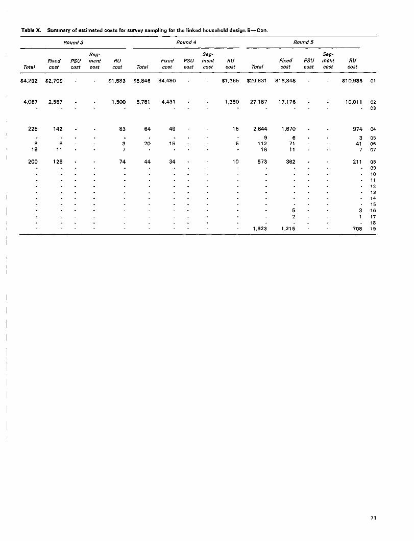
Table X. Summery of estimeted coste for survey sampling for the linked household design B—Con.


Seg- Seg- Seg-

Fixed PSU menr RU Fixed PSU ment RU Fixed PSU ment RU


$4,292 .$2,709 $1,583 $5,845 $4,480 - $1,365 $29,831 $18,846 $10,985 01

4,067 2,567 1,500 5,781 4,431 -. .

1,350 27,187 17,176 10,011 0203

225

818

200

.

142

511

126

83

37

74

49 - 15 2,644

9112

18

1,670

67111

362

52

1,215

64 974

341

7

211

31

708

04

05. .15 - 520 06

07. .

44 34 -. .. .. .. .. .. .. .. .. .. .. .

10 573 0809101112

13

14

15

16

17

18

191,923

71

Table Xl. Summary of estimated costs for survey sampling for the linked household design C

Round 1 Round 2



01

02

03

04

05

06

07

06

09

10

11

12

13

14

15

16

17

18

19

Total . . . . . . . . . . . . . . . . . . . . . . . .


On-sits . . . . . . . . . . . . . . . . . . . . . . .Off-site . . . . . . . . . . . . . . . . . . . . . . .

Othar direct costs

Total . . . . . . . . . . . . . . . . . . . . . . . . .

Materiala and supplies.. . . . . . . . .Services . . . . . . . . . . . . . . . . . . . . . .Shipping and communications . . .Travel:

On-site . . . . . . . . . . . . . . . . . ..i.

Off-site . . . . . . . . . . . . . . . . . . . . .Consultants . . . . . . . . . . . . . . . . . . .Computer services . . . . . . . . . . . . .Raporte and reproductions. . . . . . .Interviewer servicaa . . . . . . . . . . . .

Interviewer expenses ., . . . . . . . . .Respondent incentives. . . . . . . . . .Clarical labor . . . . . . . . . . . . . . . . . .Clerical labor surcharge . . . . . . . . .Miscellaneous . . . . . . . . . . . . . . . . .

Overtime expenses l., c.,.,.....

$72,690

64,593

8,105

241456441

1,043

2,915545

2,468

$19,742

15,688

4,060

229279107

2,905

541

$3,111

2,472

640

71

45885

$9,909

7,474

1,934

109133

51

1,384258

$7,228

5,742

1,486

84102

39

1,063

198

$2,269

1,981

288

2S8

$556

485

71

71

$1,713

1,496

217

217

NOTES Number of primary sampling units (PSU’S) = 100; numbar of segments = 1,629; RU = reporting unit.

Round Round Round Round Round[tern 1 2 3 4 5

Completad personsl

interviews. . . . . . . . . . . . 10,290 10,154 1,729 853 10,225

Completed telephone

interviews . . . . . . . . . . . . 8,443 6,252

72

Table Xl. Summary of astimatad costs for survey sampling for the linked household design C—Con.


Seg- Sep Seg-

Fixed PSU ment RU Fixed PSU ment RU Fixed PSU ment RU


$5,509

5,221

289

1023

256

$2,709

2,567

142

511

126

$2,600 $6,895

6,820

76

23

52

$4,480

4,431

49

15

34

$2,415 $38,275

34,883

3,392

12

14423

735

104

2,468

$18,846 $19,429 01

0203

04

05

0607

080910111213141516171819

2,654 2,389 17,176 17,707

147 27 1,670 1,722

6

7312

6

7111

8512

130 16 362 373

52

1,215

52

1,253

73

Table X11. Summary of estimated costs for survey sempling for the Iinkad household design D

Round 1 Round 2

Seg- Seg-

Fixed Psu ment RU Fixed PSU ment RU


01

0203

04

050607

0809101112

13141516171819

Total . . . . . . . . . . . . . . . . . . . . . . . . .


On-site . . . . . . . . . . . . . . . . . . . . . . .Off-site . . . . . . . . . . . . . . . . . . . . . . .

Other direct costs

Total. . . . . . . . . . . . . . . . . . . . . . . . .

Materials and supplies . . . . . . . . . .Services . . . . . . . . . . . . . . . . . . . . . .Shipping and communication . . .Travel:

On-sits . . . . . . . . . . . . . . . . . . . . .Off-site . . . . . . . . . . . . . . . . . . . . .

Consultants . . . . . . . . . . . . . . . . . . .Computer services . . . . . . . . . . . . .Reporta and reproductions. , , . . . .Interviewer services . . . . . . . . . . . .Interviewer expenaea ., . . . . . . . . .Respondent incentives. . . . . . . . . .Clerical labor . . . . . . . . . . . . . . . . . .Clerical labor surcharge . . . . . . . . .Miscellaneous . . . . . . . . . . . . . . . . .Overtime expensaa . . . . . . . . . . . . .

$69,002

61,373

7,632

226428413

999

2,704505

2,360

$18,318

14,553

3,766

214259

99

2,695502

$3,111

2,472

640

364417

45885

$8,600

6,832

1,768

100122

46

1,265236

$6,607

5,249

1,358

769336

972181

$2,122

1,852

270

270

$556

485

71

71

$1,566

1,367

199

.

199

.

.

.

NOTES Number of prima~ sampling units (PSU’S) = 200; number of segments = 1,469; RU = reporting unit.


Completed perscmalinterview s. . . . . . . . . . . . 9,406 9,262 1,580 779 9,346

Completed telsphoneinterviews .,.,......,.. 7,717 5,716 -

74

Table XII. Summary of estimated costs for survey sampling for the linked household design D—Con.


Seg- Seg- Seg-

Fixed PSU ment RU Fixed PSLJ ment RU Fixed PSU ment RUTotal cost cost cost cost Total cost cost cost cost Total cost cost cost cost

$5,269 $2,709

2,567

142

511

126

$2,560

2,426

$6,688

6,614

76

23

51

$4,480 $2,208

2,183

24

8

17

$36,605 $18,846 - -

17,176 - -

$17,759 01

0203

04

4,993 4,431 33,361 16,185. .

276 49 3,244

12

13722

703

2,360

134 1,670

6

7111

1,574

6

6611

341

41

1,145

05

411

15922

0607

08245 119 34 36209

10

111213141516171819

.

52

1,215

75

Our warehouses here at the GovernmentPrinting Office contain more than 16,000different Government publications. Nowwe’ve put together a catalog of nearly1,000 of the most popular books in ourinventory. Books like Infant Care,National Park Guide and Map, TheSpace Shuttle at Work, Federal Benefits

Talents, and The Back-Yard Mechanic.Books on subjects ranging fromagriculture, business, children,and diet to science, space exploration,transportation, and vacations. Find outwhat the Government’s books are allabout. For your free copy of ournew bestseller catalog, write—

for Veterans and Dependents,~e~g~~e;;Merchandising Your Job

&@##@zw.?w&lw:..

..-.

. ...—.. — .. .. .. .. ..

,/”4

ISN’T EASY!

In today’s health worldg nohealth professional can affordto fall behind. Let us help.Public Health Reports - the journal of theU.S. Public Health Service - brings together inone convenient source information you need onFederal health policies, innovative programs andservices of public and private agencies, researchin health fields and public health around the world.

Your subscription will bring you six wide-ranging issues a year-each one includingmore than a dozen peer-reviewed papers byrecognized authorities in health and relatedfields, thought-provoking commentary on healthissues and timely information on the preventionand control of disease,The cost of all this? Only $21 a year.Don’t miss an issud Subscribe now. Justcomplete and mail the coupon below,

To:mwyK*nt of Documents

US. “GovwnrrmtPrintingOfficeWasbirtgton,D.c.20402

NunO-mst I.ml

I II IllSwmtmMr0a8

I II 1111 I IJcmww-u~addmum

1111 HHll Hl~JJ._LL..Clly

II I I II I 111(w CumtfYi

1 Ill II I Ill

El YES!— ——!iertdmePUtWCHEALIHREPORTS(HSMHA) for m year.

Cl ldere’smy check for $ , rm% out to “mdti of DOWmmta”@@ctiPibn$ we $21 per year dorne$itiq $2(3.75 f@##rU

Cl Charge my— WC) DepositAccount mIII13a

—wa— Maetemard ~ ~-

Vital and Health Statisticsseries descriptions

SERIES 1.

SERIES 2.

SERIES 3.

SERIES 4.

SERIES 5.

SERIES 10.

SERIES 11.

SERIES 12.

SERIES 13.

Programs and Collection Procedures—Reports describing

the general programs of the National Center for Health

%3dStlCS and its offices and divisions and the data COI.

Iection methods used. They also include definitions and

other material necessary for understanding tha data.

Data Evaluation and Methods Research—Studies of new

statistical methodology including experimental tests of

new survey methods, studies of vital statistics collection

methods, new analytical techniques, objective evaluations

of reliability of collected data, and contributions to

statistical theory. Studies also include comparison of

U.S. methodology with those of other countries.

Analytical and Epidemiological Studies-Reports pre-

senting analytical or interpretive studies baaed on vital

and health statistics, carrying the analysis further than

the expository types of reports in the other series.

Documents and Committee Reports-Final reports of

mtqor committees concerned with vital and health sta-

tistics and documents such as recommended model vital

mglstration laws and revised birth and death certificates.

Compwativa International Vital and Health Statistics

Rapmts—Analytical and descriptwe reports comparing

U.S. vital and health statistics with those of other countnes.

Data From the National Health Intarview Survey- Statm-

tics on illness, accidental Injuries, disability, use of hos-

pital, medical, dental, and other services, and other

health-related topics, all based on data collected in the

continuing national household interview survey.

Data From the National Health Examination Survay and

the National Health and Nutrition Examination Survey—

Data from direct examination, tasting, and measurement

of national samples of the civilian noninstitutlona lized

population provide the basis for (1) estimates of the

medically daflned prevalence of specific diseases m the

United States and the distributions of the population

with respect to physical, physiological, and psycho-

logical characteristics and (2) analysis of relatlonshlpa

among the varioua measurements without reference to

cm explicit finite universe of persons.

Data From the Institutionalized Population Surveya-Dls-

contlnued in 1975. Reports from these surveys are in-

cluded in Series 13.

Data on Health Resources Utilization—Statistics on the

utilization of health manpower and facilities provldlng

long-term care, ambulato~ care, hospital csre, and fam[ly

planning swvices.

SERIES 14.

SERIES 15.

SERIES 20.

SERIES 21.

SERIES 22.

SERIES 23.

Data on Health Resources: Menpower and Facilities—

Statmtlcs on the numbers, geographic distribution, and

characteristics of health resources mcludlng physicians,

dentists, nurses, other health occupations, hospitals,

nursing homes, and outpatient facilities.

Data From Special Surveys-Statistics on health and

health-relatad topics collected In special surveys that

are not a part of the continuing data systems of the

National Center for Health Statistics.

Date on Mortality-Various statistics on mortal[ty other

than aa included m regular annual or monthly reports.

Special analyses by cause of death, age, and other demo-

graphic variables; geographic and time series analyses;

end statistics on characteristics of deaths not availablefrom the vital records based on sample surveys of those

records.

Data on Natelity, Merriage, and Divorca—Various sta-

W.tics on natal[ty, marriage, and divorce other than as

included In regular annual or monthly reports. Special

analyses by demographic variables; geographic and time

series analyses; studlea of fertlllty; and statistics on

characterratlcs of births not available from the wtal

records based on sample surveys of those records.

Data From the National Mortelity and Natality Surveys—

Discontinued In 1975. Reports from these sample surveys

based on vital records are included in Series 20 and 21,

respectwely.

Data From the National Survey of Family Grovvth—

Stattstlcs on ferollty, fam!ly formatton and dissolution,

family plannlng, and related maternal and infant health

topics darived from a periodic survey of a nattonwlde

probability sample of women 15–44 years of age.

For answers to quest!ons about this report or for a Ilst of titles of

reports published In these series, contace

Sclent[flc and Technical Information Branch

National Center for Health Stat] sttcsPubllc Health Serwce

Hyattsville, Md. 20782

301-436-8500

U.S. DEPARTMENT OF HEALTH ANDHUMAN SERVICES

Public Health SewiceNational Center for Health Statistics3700 East-West HighwayHyattsville, Maryland 20782

OFFICIAL 8USINESSPENALTY FOR PRIVATE USE, $300

THIRD CLASS MAIL8ULK RATE

POSTAGE & FEES PAIDPHS/NCHS

PERMIT No. G-281

DHHS Publication No. (PHS) 87-1375, Series 2, No. 101