national open university of nigeria school …nouedu.net/sites/default/files/2017-03/fmt 312.pdf ·...
TRANSCRIPT

NATIONAL OPEN UNIVERSITY OF NIGERIA
SCHOOL OF SCIENCE AND TECHNOLOGY
COURSE CODE: FMT 312
COURSE TITLE: MATHEMATICAL PROGRAMMING II

MATHEMATICAL PROGRAMMING II
FMT 312
Course Guide
Course Developer/Writer: Prof. U.A.OSISIOGU Mathematics Department,
Eboyin State University,
Eboyin State
Course Editor: Dr. AJIBOLA Saheed. O
School of Science and Technology
National Open University of Nigeria.
and
Prof. M.O. Ajetunmobi
Mathematics Department,
Lagos State University, Ojo.
Programme Leader: Dr. AJIBOLA Saheed. O
School of Science and Technology
National Open University of Nigeria.
Course Coordinator:

CONTENT
Introduction
Course Aim
Course Objectives
Study Units
Assignments
Tutor Marked Assignment
Final Examination and Grading
Summary

INTRODUCTION
You are holding in your hand the course guide for FMT 312 (Linear Programming II). The
purpose of the course guide is to relate to you the basic structure of the course material you
are expected to study. Like the name ‘course guide’ implies, it is to guide you on what to expect
from the course material and at the end of studying the course material.
COURSE CONTENT
Non – linear programming, quadratic programming Kuhntucker methods, optimality criteria
simple variable optimization. Multivariable techniques, Gradient methods.
COURSE AIM
The aim of the course is to bring to your cognizance the different methods of solving (Non-LPP)
thus Non-Linear programming models in Finance as mentioned in the course content to handle
Financial problems via the use of Statistics and calculations.
COURSE OBJECTIVES
At the end of studying the course material, among other objectives, you should be able to: (i) Define continuous functions, differentiability and continuous differentiable function
in Rn. (ii) Define and use the concept of partial derivatives and directional derivatives.
(iii) Find Higher order Derivatives of a function defined on a subset S of Rn.
(iv) Define quadratic forms and Definiteness.
(v) Identify definiteness and semidefiniteness.
COURSE MATERIAL
The course material package is composed of:
The Course Guide
The study units
Self-Assessment Exercises
Tutor Marked Assignment
References/Further Reading
THE STUDY UNITS
There are two modules and four units in this course material.
These study units are as listed below:
MODULE I
CLASSICAL OPTIMIZATION THEORY IN RN

UNIT I Basic Concepts of Rn
UNIT 2
Optimization in Rn UNIT 3
MODULE II
Unconstrained Optimization
UNIT 4
Constrained Optimization TUTOR MARKED ASSIGNMENTS
The Tutor Marked Assignments (TMAs) at the end of each unit are designed to test your
knowledge and application of the concepts learned. Besides the preparatory TMAs in the
course material to test what has been learnt, it is important that you know that at the end of
the course, you must have done your examinable TMAs as they fall due, which are marked
electronically. They make up to 30 percent of the total score for the course.
SUMMARY Having gone through this course, you now know
(i) A Typical Optimization Problem is
Minimize(or Maximize) f(x) Subject to: x ∈ D
where f : D ⊂ R → R is called the objective function and D is called the constraint set.
(ii) Optimization problems are of two types, namely Constrained and Unconstrained
Prob- lems. It is constrained if the constraint set D is made up of a set of inequalities
and/or equations (iii) If for example in the problem min( or max) f(x) subject to x ∈ D that f is continuous and D is a bounded and closed subset ofRn, the there exist a solution
for the problem. This is the Weierstrass Existence theorem theorem. (iv) A real valued
function f : Rn → R is coercive if you have
lim kxk→+∞
f(x) = +∞.

(v) If f is continuous and coercive on a closed set D ⊂ R then there exist ¯ x ∈ D such
that f(¯ x) ≤ f(x) for all x ∈ D.
(ii) the existence theorems for solution of an optimization problem.
Good luck.

FMT 313
MATHEMATICAL PROGRAMMING II
Prof.U.A. OSISIOGU

1
CONTENTS
I CLASSICAL OPTIMIZATION THEORY IN RN 4
1 Basic Concepts of Rn 5
1.1 Introduction . . . . . . . . . . . . . . . . . . . . . . . . . . . . . . . . . . . . 5
1.2 Objectives . . . . . . . . . . . . . . . . . . . . . . . . . . . . . . . . . . . . . 5
1.3 Functions . . . . . . . . . . . . . . . . . . . . . . . . . . . . . . . . . . . . . 6
1.3.1 Continuous Functions . . . . . . . . . . . . . . . . . . . . . . . . . . 6
1.3.2 Differentiable and Continuously Differentiable Functions . . . . . . . . 7
1.3.3 Partial Derivatives and Differentiability . . . . . . . . . . . . . . . . . 10
1.3.4 Directional Derivatives and Differentiability . . . . . . . . . . . . . . . 12
1.3.5 Higher Order Derivatives . . . . . . . . . . . . . . . . . . . . . . . . . 13
1.4 Quadratic Forms: Definite and Semidefinite Matrices . . . . . . . . . . . . . . 14
1.4.1 Quadratic Forms and Definiteness . . . . . . . . . . . . . . . . . . . . 14
1.4.2 Identifying Definiteness and Semidefiniteness . . . . . . . . . . . . . . 17
1.5 Some Important Results . . . . . . . . . . . . . . . . . . . . . . . . . . . . . . 19
1.5.1 Separation Theorems . . . . . . . . . . . . . . . . . . . . . . . . . . . 19
1.5.2 The Intermediate and Mean Value Theorems . . . . . . . . . . . . . . 21
1.5.3 The Inverse and Implicit Function Theorems . . . . . . . . . . . . . . 25
1.6 Conclusion . . . . . . . . . . . . . . . . . . . . . . . . . . . . . . . . . . . . 27
1.7 Summary . . . . . . . . . . . . . . . . . . . . . . . . . . . . . . . . . . . . . 27
1.8 Tutor Marked Assignments . . . . . . . . . . . . . . . . . . . . . . . . . . . . 27
Ref erences . . . . . . . . . . . . . . . . . . . . . . . . . . . . . . . . . . . . . . . . 30

2
CONTENTS CONTENTS
2 Optimization in Rn 32
2.1 Introduction . . . . . . . . . . . . . . . . . . . . . . . . . . . . . . . . . . . . 32
2.2 Objectives . . . . . . . . . . . . . . . . . . . . . . . . . . . . . . . . . . . . . 32
2.3 Main Content . . . . . . . . . . . . . . . . . . . . . . . . . . . . . . . . . . . 32
2.3.1 Optimization problems in Rn . . . . . . . . . . . . . . . . . . . . . . . 32
2.3.2 Types of Optimization problem . . . . . . . . . . . . . . . . . . . . . 35
2.3.3 The Objectives of Optimization Theory . . . . . . . . . . . . . . . . . 36
2.4 Existence of Solutions: The Weierstrass Theorem . . . . . . . . . . . . . . . . 36
2.4.1 The Weierstrass Theorem . . . . . . . . . . . . . . . . . . . . . . . . 37
2.5 Conclusion . . . . . . . . . . . . . . . . . . . . . . . . . . . . . . . . . . . . 41
2.6 Summary . . . . . . . . . . . . . . . . . . . . . . . . . . . . . . . . . . . . . 42
2.7 Tutor Marked Assignments(TMAs) . . . . . . . . . . . . . . . . . . . . . . . 42
References . . . . . . . . . . . . . . . . . . . . . . . . . . . . . . . . . . . . . . . . 43
3 Unconstrained Optimization 44
3.1 Introduction . . . . . . . . . . . . . . . . . . . . . . . . . . . . . . . . . . . . 44
3.2 Objectives . . . . . . . . . . . . . . . . . . . . . . . . . . . . . . . . . . . . . 44
3.3 Main Content . . . . . . . . . . . . . . . . . . . . . . . . . . . . . . . . . . . 45
3.3.1 Gradients and Hessians . . . . . . . . . . . . . . . . . . . . . . . . . . 45
3.3.2 Local, Global and Strict Optima . . . . . . . . . . . . . . . . . . . . . 46
3.3.3 Optimality Conditions For Unconstrained Problems . . . . . . . . . . . 46
3.3.4 Coercive functions and Global Minimizers . . . . . . . . . . . . . . . 53
3.4 Convex Sets and Convex Functions . . . . . . . . . . . . . . . . . . . . . . . . 54
3.4.1 Convex Sets . . . . . . . . . . . . . . . . . . . . . . . . . . . . . . . . 54
3.4.2 Convex Functions . . . . . . . . . . . . . . . . . . . . . . . . . . . . . 56
3.4.3 Convexity and Optimization . . . . . . . . . . . . . . . . . . . . . . . 57
3.5 Conclusion . . . . . . . . . . . . . . . . . . . . . . . . . . . . . . . . . . . . 63
3.6 Summary . . . . . . . . . . . . . . . . . . . . . . . . . . . . . . . . . . . . . 63
3.7 Tutor Marked Assignments (TMAs) . . . . . . . . . . . . . . . . . . . . . . . 64
References . . . . . . . . . . . . . . . . . . . . . . . . . . . . . . . . . . . . . . . . 66
4 Constrained Optimization 67
4.1 Introduction . . . . . . . . . . . . . . . . . . . . . . . . . . . . . . . . . . . . 67
4.2 Objectives . . . . . . . . . . . . . . . . . . . . . . . . . . . . . . . . . . . . . 67

3
CONTENTS CONTENTS
4.3 Constrained Optimization Problem . . . . . . . . . . . . . . . . . . . . . . . . 67
4.4 Equality-Constraint . . . . . . . . . . . . . . . . . . . . . . . . . . . . . . . . 69
4.4.1 Lagrangian . . . . . . . . . . . . . . . . . . . . . . . . . . . . . . . . 71
4.4.2 General Formulation . . . . . . . . . . . . . . . . . . . . . . . . . . . 73
4.5 Inequality Constraints . . . . . . . . . . . . . . . . . . . . . . . . . . . . . . . 76
4.6 Conclusion . . . . . . . . . . . . . . . . . . . . . . . . . . . . . . . . . . . . 76
4.7 Summary . . . . . . . . . . . . . . . . . . . . . . . . . . . . . . . . . . . . . 77
4.8 Tutor Marked Assignments(TMAs) . . . . . . . . . . . . . . . . . . . . . . . 77
References . . . . . . . . . . . . . . . . . . . . . . . . . . . . . . . . . . . . . . . . 78

4
Module I
CLASSICAL OPTIMIZATION THEORY
IN RN

5
UNIT 1
BASIC CONCEPTS OF RN
1.1 Introduction
In this unit and subsequent units, you shall be considering another aspect of optimization prob-
lems, different from the linear programming problem you have seen in previous units. The
theorems you shall develop here are more general to any given mathematical programming in
which the objective function f : S ⊂ Rn → R defined on a subset S of Rn is nonlinear. Also the constraints may or may not be linear in the decision variables and the non-negativity condition is also relaxed.
For a better understanding of optimization in Rn, you shall, in this unit, be introduced to
some basic concepts and notions of the space Rn (also known as the real n-space). These no-
tions, can also be referred to as the topology of Rn. Thus, you shall be considering notions like, Continuous functions, differentiability, partial derivatives, directional derivatives and higher or-
der derivatives. You will also consider quadratic forms: definite and semidefinite matrices and also see some results.
1.2 Objectives
At the end of this unit, you should be able to
(i) Define continuous functions, differentiability and continuous differentiable function in
Rn.
(ii) Define and use the concept of partial derivatives and directional derivatives.
(iii) Find Higher order Derivatives of a function defined on a subset S of Rn.
(iv) Define quadratic forms and Definiteness.

6
UNIT 1. BASIC CONCEPTS OF RN 1.3 Functions
(v) Identify definiteness and semidefiniteness.
1.3 Functions
Let S, T be subsets of Rn and Rl , respectively. A function f from S to T denoted by f : S → T ,
is a rule that associates with each element of S, one and only one element of T . The set S is
called the domain of the function f, and the set T is the range of the function f .
1.3.1 Continuous Functions
Definition 1.3.1 Let f : S → T , where S ⊂ Rn and T ⊂ Rl . Then, f is said to be continuous
at x ∈ S if for all > 0, there exists a δ > 0 such that y ∈ S and d(x, y) < δ implies that d(f (x), f (y)) < . (Note that d(x, y) is the distance between x and y in Rn, while d(f (x), f (y))
is the distance in Rl .)
Another way you can define continuous function is by using sequences.
Definition 1.3.2 The function f : S → T is continuous at x ∈ S if for all sequences {xk } such
that xk ∈ S for all k, and lim xk = x, then lim f (xk ) = f (x). k→∞ k→∞
Intuitively, f is continuous at x if the value of f at any point y that is “close” to x is a good
approximation of the value of f at x.
Definition 1.3.3 (Discontinuous Function) f : S → T is called discontinous at x ∈ S if it is
not continuous at x.
Example 1.3.1 (Continuous function) The identity function f (x) = x for all x ∈ R is contin-
uous at each x ∈ R
Example 1.3.2 The function f : R → R given by
0, x ≤ 0
f (x) = 1, x > 0
is continuous everywhere except at x = 0. At x = 0, every open ball B(x, δ) with center x
and radius δ > 0 contains at least one point y > 0. At all such points, f (y) = 1 > 0 = f (x),
and this approximation does not get better, no matter how close y gets to x (i.e., no matter how
small you take δ to be).
Definition 1.3.4 A function f : S → T is said to be continuous on S if it is continuous at each
point in S.
Observe that if f :⊂ Rn → Rl , then f consists of l “component functions” (f 1 , . . . , f l ),
i.e., there are functions f i : S → R, i = 1, . . . , l, such that for each x ∈ S, you have f (x) = (f 1(x), . . . , f l (x)).

7
UNIT 1. BASIC CONCEPTS OF RN 1.3 Functions
Proposition 1.3.1 f is continuous at x ∈ S (resp. f is continuous on S) if and only if each f i is continuous at x (resp. if and only if each f i is continuous on S).
Theorem 1.3.1 A function f : S ⊂ Rn → Rl is continuous at a point x ∈ S if and only if for
all open set V ⊂ Rl such that f (x) ∈ V, there is an open set U ⊂ Rn such that x ∈ U, and f (z) ∈ V for all z ∈ U ∩ S.
Proof. Suppose f is continuous at x, and V is an open set in Rl containing f (x). Suppose, by contradiction, that the theorem was false, so for any open set U containing x, there is y ∈ U ∩ S such that f (y) ∈ V. Let k ∈ {1, 2, 3, . . . }, let Uk be the open ball with center
x and radius 1/k. Let yk ∈ Uk ∩ S be such that f (yk ) ∈ V. The sequence {yk } is clearly
well defined, and since yk ∈ Uk for all k, you have d(x, yk ) < 1/k for each k, so yk → x as k
→ ∞. Since f is continuous at x by hypothesis, you also have f (yk ) → f (x) as k → ∞.
However f (yk ) ∈ V for any k, and since V is open, V c is closed, so f (x) = lim f (yk )
∈ V c which contradicts
f (x) ∈ V. k→∞
Conversely, suppose that for each open set V containing f (x), there is an open set U con- taining x such that f (y) ∈ V for all y ∈ U ∩ S. You will show that f is continuous at x. Let
> 0 be given. Define V to be the open ball in Rl with center f (x) and radius . Then, there exists an open set U containing x such that f (y) ∈ V for all y ∈ U ∩ S. Pick any δ > 0
so that B(x, δ) ∈ U . Then, by construction, it is true that y ∈ S and d(x, y) < δ implies f (y) ∈ V , i.e., that d(f (x), f (y)) < . Since > 0 is arbitrary, you have shown precisely that f is continuous at x.
As an immediate corollary, you have the following statement, which is usually abbreviated
as: “a function is continuous if and only if the inverse image of every open set is open.”
Corollary 1.3.1 A function f : S ⊂ Rn → Rl is continuous on S if and only if for each open
set V ⊂ Rl , there is an open set U ⊂ Rn such that f − 1 (V ) = U ∩ S where f − 1 (V ) is defined by
f − 1 (V ) = {x ∈ S|f (x) ∈ V }
In particular, if S is an open set in Rn, f is continuous on S if and only if f − 1 (V ) is an open
set in Rn for each open set V in Rl .
Finally, some observation. Note that continuity of a function f at a point x is a local prop-
erty, i.e., it relates to the behaviour of f near x. but tells you nothing about the behaviou of f
elsewhere. In particular, the continuity of f at x has no implicatioin even for the continuity of
f at points “close” to x. Indeed, it is easy to construct functions that are continuous at a given
point x, but that are discontinous at every neighbourhood of x. It is also important to note that,
in general, functions need not be continuous at even a single point in their domain. Consider
f : R+ → R+ given by f (x) = 1, if x is a rational number, and f (x) = 0, otherwise. This function is discontinuous everywhere on R+ .
1.3.2 Differentiable and Continuously Differentiable Functions
Throughout this subsection, S will denote an open set in Rn

8
UNIT 1. BASIC CONCEPTS OF RN 1.3 Functions
Definition 1.3.5 (Differentiability) A function f : S → Rm is said to be differentiable at a
point x ∈ S if there exists an m × n matrix A such that for all > 0, there is δ > 0 such that
y ∈ S and x − y < δ implies
f (x) − f (y) − A(x − y) < x − y
.
Equivalently, f is differentiable at x ∈ S if
( \
lim y→x
f (y) − f (x) − A(y − x) = 0
y − x
(The notation “y → x” is shorthand for “ for all sequences {yk } such that yk → x.”)
The matrix A in this case is called derivative of f at x and is denoted Df (x). Figure 1.1
provides a graphical illustration of the derivative. In keeping with standard practice, you shall,
in the sequel, denote Df (x) by f !(x) whenever n = m = 1, i.e., whenever S ⊂ R and f : S → R.
g ( y )=a +by f ( y)
f ( x )
x
Figure 1.1: The Derivative
Remark 1.3.1 The definition of the derivative Df may be motivated as follows. An affine func-
tion from Rn to Rm is a function g is of the form
g(y) = Ay + b,

9
UNIT 1. BASIC CONCEPTS OF RN 1.3 Functions
x2
where A is an m × n matrix, and b ∈ Rm. (When b = 0, the function g is called linear.)
Intuitively, the derivative of f at a point x ∈ S is the best affine approximation to f at x, i.e.,
the best approximation of f around the point x by an affine function g. Here, “best” means that
the ratio
( \ f (y) − g(y)
y − x
goes to zero as y → x. Since the values of f and g must coincide at x (otherwise g would be hardly be a good approximation to f at x), you must have g(x) = Ax + b = f (x), or b = f (x) − Ax. Thus, you may write this approximating function g as
g(y) = Ay − Ax + f (x) = A(y − x) + f (x).
Given this value for g(y), the task of identifying the best affine approximation to f at x now
amounts to identifying a matrix A such that
( \ ( f (y) − g(y)
= y − x
f (y) − (A(y − x)) + f (x)
y − x
\
→ 0 as y → x.
This is precisely the definition of the derivative you have given.
If f is differentiable at all points in S, then f is said to be differentiable on S. When f is differentiable on S, the derivative Df itself forms a function from S to Rm×n. If Df : S →
Rm×n is a continuous function, then f is said to be continuously differentiable on S, and you
write f is C 1.
The following observations are immediate from the definitions. A function f : S ⊂ Rn → Rm is differentiable at x ∈ S if and only if each of the m componet functions f i : S → R of f is differentiable at x, in which case you have Df (x) = (Df 1(x), . . . , Df m(x)). Moreover, f is
C 1 on S if and only if each f i is C 1 on S.
The difference between differentiability and continuous differentiability is non-trivial. The
following example shows that a function may be differentiable everywhere, but may still not be
continuously differentiable.
Example 1.3.3 Let f : R → R be given by
f (x) = 0, if x = 0
( ) x2 sin 1
if x = 0.
For x = 0, you have
( \ ( \
f ! (x) = 2x sin 1 2 1
x2 −
x cos
x2 .
Since | sin(·)| ≤ 1 and | cos(·)| ≤ 1, but (2/x) → ∞ as x → 0, it is clear that the limit as x → 0
of f !(x) is not well defined. However, f !(0) does exist! Indeed, (
f !(0) = lim x→0
\ f (x) − f (0)
x − 0
( \ 1
= lim x sin . x→0 x2

UNIT 1. BASIC CONCEPTS OF RN 1.3 Functions
1
Since | sin(1/x2 )| ≤ 1, you have |x sin(1/x2 )| ≤ |x|, so x sin(1/x2 ) → 0 as x → 0. This means f !(0) = 0. Thus, f is not C 1 on R+ .
This example notwithstanding, it is true that the derivative of everywhere differentiable
function f must possess a minimal amount of continuity. This you shall see in the intermediate
value theorem later in this unit.
You shall close this subsection with a statement of two important properties of the derivative. First, given two functions f : Rn → Rm and g : Rn → Rm, define their sum (f + g) to be the
function from Rn to Rm whose value at any x ∈ Rn is f (x) + g(x).
Theorem 1.3.1 If f : Rn → Rm and g : Rn → Rm are both differentiable at a point x ∈ Rn,
so is (f + g) and, in fact,
D(f + g)(x) = Df (x) + Dg(x).
Proof. Obvious from the definition of differentiability.
Next, given functions f : Rn → Rm and h : Rk → Rn, define, their composition f ◦ h to
be the function from Rk to Rm whose value at any x ∈ Rk is given by f (h(x)), that is, by the
value of f evaluated at h(x).
Theorem 1.3.2 Let f : Rn → Rm and h : Rk → Rn. Let x ∈ Rk . If h is differentiable at x,
and f is differintiable at h(x), the f ◦ h is itself differetiable at x, and its derivative may be
obtained throughout the “chain rule” as:
D(f ◦ h)(x) = Df (h(x))Dh(x).
Proof. See Rudin (1976, theorem 9.15, p.214).
Theorems 1.3.1 and 1.3.2 are only one-way implications. For instance, while the differen- tiability of f and g at x implies the differentiability of (f + g) at x, (f + g) can be differentiable
everywhere (even C 1) without f and g being differentiable anywhere. For an example, let
f : R → R be given by f (x) = 1 if x is rational, and f (x) = 0 otherwise, and let g : R → R be given by g(x) = 0 if x is rational, and g(x) = 1 otherwise. Then, f and g are discontinuous everywhere, so are certainly not differentiable anywhere. However, (f + g)(x) = 1 for all x, so
(f + g)!(x) = 0 at all x, meaning (f + g) is C 1. Similarly, the differeintiability of f ◦ h has no implications for the differentiability of f at h(x) or the differentiability of h at x.
1.3.3 Partial Derivatives and Differentiability
Definition 1.3.6 Let f : S → R, where S ⊂ Rn is an open set. Let ej denote the vector in Rn
that has a 1 in the j − th place and zeros elsewhere (j = 1, . . . , n). Then the j − th partial derivative of f is said to exist at a point x if there is a number ∂ f (x)/∂xj such that
(
lim t→0
\ f (x + tej ) − f (x)
t
∂f =
∂xj
(x)
Among the more pleasant facts of life are the following:

UNIT 1. BASIC CONCEPTS OF RN 1.3 Functions
1
Theorem 1.3.3 Let f : S → R, where S ⊂ Rn is open.
1. If f is differentiable at x, then all partials ∂ f (x)/∂ xj exist at x, and
Df (x) = [∂ f (x)/∂ x1 , . . . , ∂ f (x)/∂ xn]
2. If all the partials ∂f (x)/∂ xj exist and are continuous at x, then Df (x) exists and
Df (x) = [∂ f (x)/∂ x1 , . . . , ∂ f (x)/∂ xn]
3. f is C 1 on S if and only if all partial derivatives of f exist and are continuous on S.
Proof. See Rudin (1976, Theorem 9.21, p219).
Thus, to check if f is C 1, you only need figure out if (a) the partial derivatives exist on S,
and (b) if they are all continuous on S. On the other hand, the requirement that the partials not
only exist but be continuous at x is very important for the coincidence of the vector of partials
with Df (x). In the absence of this condition, all partials could exist at some point without the
function itself being differentiable at that point. Consider the following example:
Example 1.3.4 Let f : R2 → R be given by f (0, 0) = 0, and for (x, y) = (0, 0)
xy f
(x, y) = ψ . x2 + y2
You will show that f has all partial derivatives everywhere (including at (0, 0)), but that these
partials are not continuous at (0, 0). Then you have to show that f is differentiable at (0, 0).
☞ Solution. Since f (x, 0) = 0 for any x = 0, it is immediate that for all x = 0,
∂f (x, 0) = lim
f (x, y) − f (x, 0) x = lim = 1.
∂y y→0 y y→0 x2 + y2
Similarly, at all points of the form (0, y) for y = 0, you have ∂ f (0, y)/∂x = 1. However, note
that ∂f
(0, 0) = lim f (x, 0) − f (0, 0)
= lim 0 − 0
= 0, ∂x x→0 x x→0 x
so ∂ f (0, 0)/∂ x exists at (0, 0), but is not the limit of ∂f (0, y)/∂ x as y → 0. Similarly, you also have ∂ f (0, 0)/∂y = 0 = 1 = lim ∂ f (x, 0)/∂y.
x→0
Suppose f were differentiable at (0, 0). Then, the derivatives Df (0, 0) must conicide with
the vector of partials at (0, 0) so you must have Df (0, 0) = (0, 0). However, from the definition
of the derivative, you must also have
lim (x,y)→(0,0)
f (x, y) − f (0, 0) − Df (0, 0) · (x, y) = 0 (x, y) − (0, 0)
but this is impossible if Df (0, 0) = 0. To see this, take any point (x, y) of the form (a, a) for
some a > 0, and note that every neighbourhood of (0, 0) contains at least one such point. Since
f (0, 0) = 0, Df (0, 0) = (0, 0), and (x, y) = x2 + y2, it follows that
f (a, a) − f (0, 0) − Df (0, 0) · (a, a) a2 1 = =
(a, a) − (0, 0) 2a2 2

UNIT 1. BASIC CONCEPTS OF RN 1.3 Functions
1
l
so the limit of this fraction as a → 0 cannot be zero. ✍
Intuitively, the feature that drives this example is that in looking at the partial derivative of f with respect to (say) x at a point (x, y), you are moving along only the line through (x, y)
parallel to the x-axis (see the line denoted l1 in Figure 1.2). Similarly, the partial with derivative
with respect to y involves holding the x variable fixed, and moving only on the line through
(x, y) parallel to the y-axis (see the line denoted l2 in Figure 1.2). On the other hand, in looking
at the derivative Df , both the x and y variables are allowed to vary simultaneously (for instance, along the dotted curve in Figure 1.2).
Lastly, it is worth stressing that although a function must be continuous in order to be dif-
ferentiable (this is easy to see from the definitions), there is no implication in the other direction
whatsoever. Extreme examples exist of functions which are continuous on all of R, but fail to be
differentiable at even a single point. Such functions are by no means pathological; they play, for
instance, a central role in the study of Brownian motion in probability theory (with probability
one, a Brownian motion path is everywhere continuous and nowhere differentiable).
y
l 2
l
1 1
x
Figure 1.2: Partial Derivatives and Differentiability
1.3.4 Directional Derivatives and Differentiability
Let f : S → R, where S ⊂ Rn is open. Let x be any point in S, and let h ∈ Rn. The directional
derivative of f at x in the direction h is defined as
lim
( \ f (x + th) − f (x)
t→0+ t

UNIT 1. BASIC CONCEPTS OF RN 1.3 Functions
1
i
1
n
when this limit exists, and is denoted Df (x; h). (The notation t → 0+ is shorthand for t > 0,
t → 0.)
When the condition t → 0+ is replaced with t → 0, you obtain what is sometimes called
the “two-sided directional derivative.” Observe that partial derivatives are a special case of two- sided directional derivatives: when h = ei for some i, the two-sided directional derivative at x
is precisely the partial derivative ∂ f (x)/∂ xi.
In the privious subsection, it was pointed out that the existence of all partial derivatives at
a point x is not sufficient to ensure that f is differentiable at x. It is actually true that no even
the existence of all two-sided directional derivatives at x implies that f is differentiable at x.
However, the following relationship in the reverse direction is easy to show.
Theorem 1.3.4 Suppose f is differentiable at x ∈ S. Then, for any h ∈ Rn, the (one-sided)
directional derivative Df (x; h) of f at x in the direction h exists, and, in fact, you have Df (x; h) = Df (x) · h.
An immediate corollary is
Corollary 1.3.2 If Df (x) exists, then Df (x; h) = − Df (x; −
h). Remark 1.3.2 What is the relationship between Df (x) and the two-sided directional deriva-
tive of f at x in an arbitrary direction h?
1.3.5 Higher Order Derivatives
Let f be a function from S ⊂ Rn to R, where S is an open set. Throughout this sub-
section, you will assume that f is differentiable on all of S, so that the derivative Df =
[∂ f /∂ x1 , . . . , ∂ f /∂ xn] itself defines a function from S to Rn.
Suppose now that there is x ∈ S such that the derivative Df is itself differentiable at x, i.e.,
such that for each i, the function ∂ f /∂ xi : S → R is differentiable at x. Denote the partial of
∂f /∂ xi in the direction ej at x by ∂2 f (x)/∂ xj ∂xi, if i = j, and ∂2 f (x)/∂ x2 , if i = j. Then,
you say that f is twice-differentiable at x, with second derivative D2 f (x), where
∂2 f (x)
∂x2
∂2 f (x) · · · ∂x1∂xn
D2 f (x) = . . . . .
∂2 f (x) ∂2 f (x)
∂xn∂x1 · · ·
∂x2
Once again, you shall follow standard practice and denote D2 f (x) by f !!(x) whenever n = 1 (i.e., if S ⊂ R).
If f is twice-differentiable at each x in S, you say that f is twice-differentiable on S. When
f is twice-differentiable on S, and for each i, j = 1, . . . , n the cross-partial ∂2 f /∂ xi∂ xj is a
1
1.4 Quadratic Forms: Definite and Semidefinite MaUtrNicITes1. BASIC CONCEPTS OF RN
continuous function from S to R, you say that f is twice continuously differentiable on S, and
you write f is C 2.
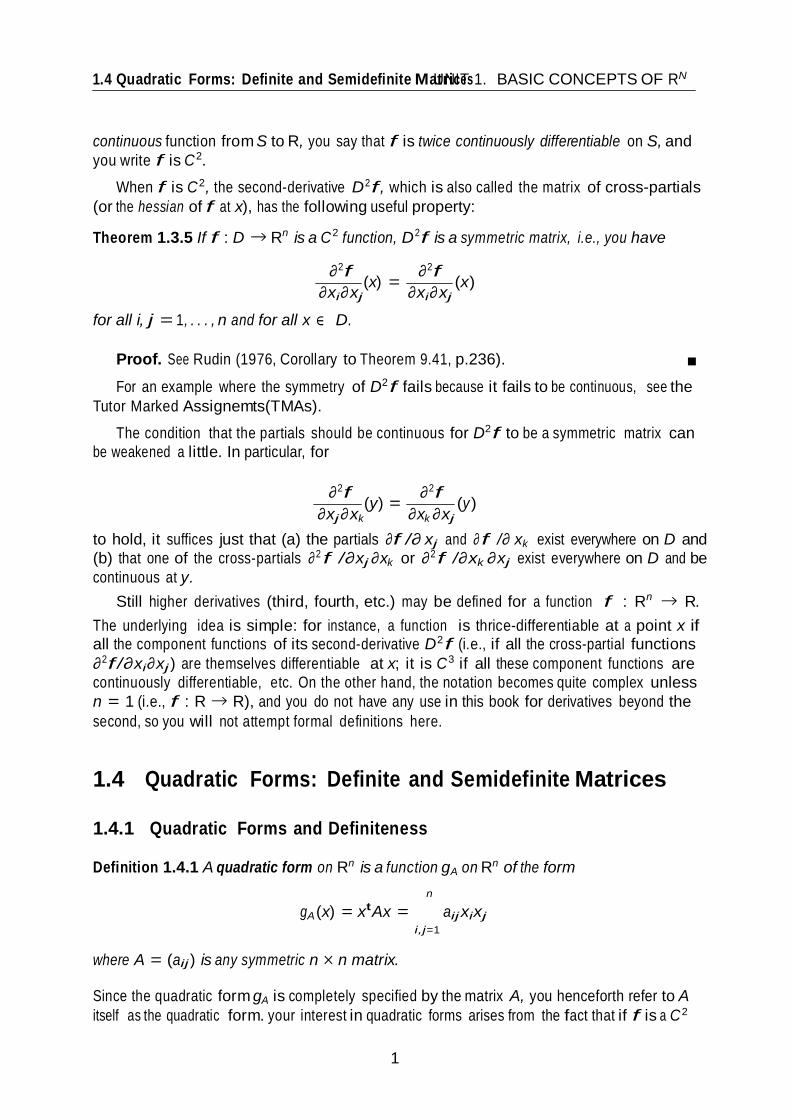
When f is C 2, the second-derivative D2 f , which is also called the matrix of cross-partials
(or the hessian of f at x), has the following useful property:
Theorem 1.3.5 If f : D → Rn is a C 2 function, D2 f is a symmetric matrix, i.e., you have
∂2 f
∂xi∂ xj
for all i, j = 1, . . . , n and for all x ∈ D.
(x) = ∂2 f
∂xi∂ xj
(x)
Proof. See Rudin (1976, Corollary to Theorem 9.41, p.236).
For an example where the symmetry of D2 f fails because it fails to be continuous, see the
Tutor Marked Assignemts(TMAs).
The condition that the partials should be continuous for D2 f to be a symmetric matrix can
be weakened a little. In particular, for
∂2 f
∂xj ∂ xk
(y) = ∂2 f
∂xk ∂xj
(y)
to hold, it suffices just that (a) the partials ∂f /∂ xj and ∂ f /∂ xk exist everywhere on D and
(b) that one of the cross-partials ∂2 f /∂xj ∂xk or ∂2 f /∂xk ∂xj exist everywhere on D and be
continuous at y.
Still higher derivatives (third, fourth, etc.) may be defined for a function f : Rn → R.
The underlying idea is simple: for instance, a function is thrice-differentiable at a point x if all the component functions of its second-derivative D2 f (i.e., if all the cross-partial functions
∂2 f /∂xi∂ xj ) are themselves differentiable at x; it is C 3 if all these component functions are
continuously differentiable, etc. On the other hand, the notation becomes quite complex unless
n = 1 (i.e., f : R → R), and you do not have any use in this book for derivatives beyond the second, so you will not attempt formal definitions here.
1.4 Quadratic Forms: Definite and Semidefinite Matrices
1.4.1 Quadratic Forms and Definiteness
Definition 1.4.1 A quadratic form on Rn is a function gA on Rn of the form
n
gA (x) = xt Ax = aij xixj
i,j=1
where A = (aij ) is any symmetric n × n matrix.
Since the quadratic form gA is completely specified by the matrix A, you henceforth refer to A
itself as the quadratic form. your interest in quadratic forms arises from the fact that if f is a C 2

1
1.4 Quadratic Forms: Definite and Semidefinite MaUtrNicITes1. BASIC CONCEPTS OF RN
1 2
function, and z is a point in the domain of f, then the matrix of second partials D2 f (z) defines
a quadratic form (this follows from Theorem 1.3.5 on the symmetry property of D2 f for a C 2
function f ).
Definition 1.4.2 A quadratic form A is said to be
1. positive definite if you have xt Ax > 0 for all x ∈ Rn, x = 0.
2. positive semidefinite if you have xt Ax ≥ 0 for all x ∈ Rn, x = 0.
3. negative definite if you have xt Ax < 0 for all x ∈ Rn, x = 0.
4. negative semidefinite if you have xt Ax ≤ 0 for all x ∈ Rn, x = 0
The terms “non-negative definite” and “nonpositive definite” are often used in place of “positive
semidefinite” and “negative semidefinite” respectively.
For instance, the quadratic form A defined by
A = 1 0
0 1
is positive definite, since for any x = (x1, x2) ∈ R2 , you have xt Ax = x2 + x2, and this quantity is positive whenever x = 0. On the other hand, consider the quadratic form
A = 1 0
0 0
2 t
For any x = (x1, x2) ∈ R2, you have xt Ax = x1 , so x Ax can be zero even if x = 0. (For
example, xt Ax = 0if x = (0, 1).) Thus, A is not positive definite. On the other hand, it is certainly true that you always have xt Ax ≥ 0, so A is positive semidefinite.
Observe that there exist matrices A which are neither positive semidefinite nor negative
semidefinite, and that do not, therefore, fit into any of the four categories you have identified.
Such matrices are called indefinite quadratic forms. As an example of an indefinite quadratic
form A, consider
A = 0 1
1 0
For x = (1, 1), xtAx = 2 > 0, so A is not negative semidefinite. But for x = (− 1, 1), xt Ax =
− 2 < 0, so A is positive semidefinite either.
Given a quadratic form A and any t ∈ R, you have (tx)t A(tx) = t2 xtAx, so the quadratic
form has the same sign along lines through the origin. Thus, in particular, A is positive definite (resp. negative definite) if and only if it satisfies xt Ax > 0 (resp. xtAx < 0) for all x in the unit sphere C = {u ∈ Rn | u = 1}. You will use this observation to show that if A is a positive definite (or negative definite) n × n matrix, so is any other quadratic form B which is sufficiently close to A.

1
1.4 Quadratic Forms: Definite and Semidefinite MaUtrNicITes1. BASIC CONCEPTS OF RN
Theorem 1.4.1 Let A be a positive definite n × n matrix. Then there is γ > 0 such that if B is any symmetric n × n matrix with |bj k − aj k | < γ for all j, k ∈ {1, . . . , n}, then B is also positive definite. A similar statement holds for negative definite matrices A.
Proof. You will make use of the Weierstrass Theorem, which will be proved later. The
Weierstrass Theorem states that if K ⊂ Rn is compact, and f : K → R is a continuous function, then f has both maximum and minimum on K, i.e., there exist points k! and k∗ in K such that f (k!) ≥ f (k) ≥ f (k∗ ) for all k ∈ K.
Now, the unit sphere C is clearly compact, and the quadratic form A is continuous on this
set. Therefore, by the Weierstrass Theorem, there is z ∈ C such that for any x ∈ C, you have
ztAz ≤ xt Ax.
If A is positive definite, then z t Az must be strictly positive, so there must exists > 0 such that
xt Ax ≥ > 0 for all x ∈ C .
Define γ = /2n2 > 0. Let B be any symmetric n×n matrix, which is such that |bj k − aj k | < γ for all j, k = 1, . . . , n. Then for any x ∈ C ,
|xt (B − A)x| = n
(b − aj k)x x
j k j k
j,k=1
n
≤ j,k=1
|bj k − aj k ||xj ||xk |
L.n
< γ j,k=1 |xj ||xk |
Therefore, for any x ∈ C ,
< γn2 = /2.
xtB x = xtAx + xt (B − A)x ≥ − /2 =
/2
so B is positive definite, and the desired result is establised.
A particular implication of this result, which you will use in the study of unconstrained
optimization problems, is the following: Corollary 1.4.1 If f is a C 2 function such that at some point x, D2 f (x) is a positive definite matrix, then there is a neighbourhood B(x, r) of x such that for all y ∈ B(x, r), D2 f (y) is also
a positive definite matrix. A similar statement holds if D2 f (x) is instead, a negative definite
matrix.
Finally, it is important to point out that Theorem 1.4.1 is no longer true if “positive definite”
is replaced with “positive semidefinite.” Consider, as a counter example, the matrix A defined
by

1
1.4 Quadratic Forms: Definite and Semidefinite MaUtrNicITes1. BASIC CONCEPTS OF RN
1 2
A = 1 0
. 0 0
You have seen above that A is positive semidefinite (but not positive definite). Pick any γ > 0.
Then, for = γ/2, the matrix
B = 1 0 0 −
satisfies |aij − bij | < γ for all i, j. However, B is not positive semidefinite: for x = (x1, x2), you
have xtB x = x2 − x2, and this quantity can be negative (for instance, if x1 = 0 and x2 = 0).
Thus, there is no neighbourhood of A such that all quadratic forms in that neighbourhood are
also positive semidefinite.
1.4.2 Identifying Definiteness and Semidefiniteness From a practical standpoint, it is of interest to ask: what restrictions on the structure of A
are imposed by the requirement that A be a positive (or negative) definite quadratic from? The
answers to this questions is provided in this section. These results are, in fact, equivalence state-
ments; that is, quadratic forms possess the required definiteness or semidefiniteness property if
and only if they meet the condition outlined.
The first result deals with positive and negative definiteness. Given an n × n symmetric
matrix A, let Ak denote the k × k submatrix of A that is obtained when only the first k rows and
columns are retained, i.e., let
a11 · · · a1k
Ak = . . . . .
ak1 · · · akk
You will refer to Ak as the k-th natural ordered principal minor of A.
Theorem 1.4.2 An n × n symmetric matrix A is
1. negative definite if and only if (− 1)k |Ak | > 0 for all k ∈ {1, . . . , n}.
2. positive definite if and only if |Ak | > 0 for all k ∈ {1, . . . , n}.
Moreover, a positive semidefinite quadratic form A is positive definite if and only if |A| = 0,
while a negative semidefinite quadratic form is negative definite if and only if |A| = 0.
Proof. See Debreu (1952, Theorem 2, p.296).
A natural conjecture is that this theorem would continue to hold if the words “negative defi-
nite” and “positive definite” were replaced with “negative semidefinite” and “positive semidef-
inite,” respectively, provided the strict inequalities were replaced with weak ones. This conjec-
ture is false. Consider the following example.

1
1.4 Quadratic Forms: Definite and Semidefinite MaUtrNicITes1. BASIC CONCEPTS OF RN
2
k
k
Example 1.4.1 Let
0 0 A =
0 1 and B =
0 0
0 − 1
Then, A and B are both symmetric matrices. Moreover, |A1 | = |A2 | = |B1 | = |B2 | = 0, so if the conjecture were true, both A and B would pass the test for positive semidefiniteness, as well as the test for negative semidefiniteness. However, for any x ∈ R2, xt Ax = x2 and
xt Bx = − x2 2. Therefore, A is positive semidefinite but not negative seimidefinite, while B is negative semidefinite, but not positive semidefinite.
Roughly speaking, the feature driving this counterexample is that, in both the matrices A
and B, the zero entries in all but the (2, 2)-place of the matrix make the determinants of order
1 and 2 both zero. In particular, no play is given to the sign of the entry in the (2, 2)-place, which is positive in one case, and negative in the other. On the other hand, an examination
of the expression xt Ax and xtB x reveals that in both cases, the sign of the quadratic form is determined precisely by the sign of the (2, 2)-entry.
This problem points to the need to expand the set of submatrices that you are considering, if
you are to obtain an analog of Theorem 1.4.2 for positive and negative semidefiniteness. Let an
n × n symmetric matrix A be given, and let π = (π1, . . . , πn) be a permutation of the integers {1, . . . , n}. Denote by Aπ the symmetric n × n matrix obtained by applying the permutation π to both the rows and columns of A :
aπ1 π1 · · · aπ1 πn
Aπ = . . . . .
aπn π1 · · · aπn πn
π π
For k ∈ {1, . . . , n}, let Ak denote the k × k symmetric submatrix of A obtained by retaining
only the first k rows and columns:
aπ1 π1 · · · aπ1 πn
π . .
Ak = .. . . .
aπk π1 · · · aπk πk
Finally, let Π denote the set of all possible permutations of {1, . . . , n}
Theorem 1.4.3 A symmetric n × n matrix A is
1. positive semidefinite if and only if |Aπ | ≥ 0 for all k ∈ {1, . . . , n} and for all π ∈ Π.
2. negative semidefinite if and only if (− 1)k |Aπ | ≥ 0 for all k ∈ {1, . . . , n} and for all
π ∈ Π.
Proof. See Debreu (1952, Theorem 7, p298).

1
UNIT 1. BASIC CONCEPTS OF RN 1.5 Some Important Results
1 2
One final remark is important. The symmetry assumptions is crucial to the validity of these
results. If it fails, a matrix A might pass all the tests for (say) positive semidefiniteness without
actually being positive semidefinite. Here are two examples:
Example 1.4.2 Let
A = 1 − 3 0 1
Note that |A1 | = 1, and |A2 | = (1)(1) − (− 3)(0) = 1, so A passes the test for positive
definiteness. However, A is not a symmetric matrix, and is not, in fact, positive definite: you have xt Ax = x2 + x2 − 3x1 x2 which is negative for x = (1, 1).
Example 1.4.3 Let
A = 0 1
. 0 0
There are only two possible permutations of the set {1, 2}, namely, {1, 2} itself, and {2, 1}.
This gives rise to four different submatrices, whose determinants you have to consider:
a11 a12 a11 a12
[a11], [a22 ], a21 a22 , and
a21
a22
You can easily check that the determinants of all four of these are non-negative, so A passes the
test for positive semidefiniteness. However, A is not positive semidefinite: you have xt Ax =
x1 x2, which could be positive or negative.
1.5 Some Important Results
This section brings together some results of importance for the study of optimization theory.
These are, the separation theorems for convex sets in Rn, consequences of assuming continu-
ity and/or differentiability of real-valued functions defined on Rn and two fundamental results known as the Inverse Function Theorem and the Implicit Function Theorem.
1.5.1 Separation Theorems
Let p = 0 be a vector in Rn, and let a ∈ R. The set H defined by
H = {x ∈ Rn|p · x = a}
is called a hyperplane in Rn, and will be denoted H (p, a).
A hyperplane in R2, for example, is simply a straight line: if p ∈ R2 and a ∈ R, the
hyperplane H (p, a) is simply the set of points (x1, x2) that satisfy p1 x1 + p2 x2 = a. Similary, a
hyperplane in R3 is a plane.
A set D in Rn is said to be bounded by a hyperplane H (p, a) if D lies entirely on one side
of H (p, a), i.e., if either

UNIT 1. BASIC CONCEPTS OF RN 1.5 Some Important Results
2
+
p · x ≤ a, for all x ∈ D
or
p · x ≥ a, for all x ∈ D
If D is bounded by H (p, a) and D ∩ H (p, a) = ∅ , then H (p, a) is said to be a supporting hyperplane for D.
Example 1.5.1 Let D = {(x, y) ∈ R2 |xy ≥ 1}. Let p be the vector (1, 1), and let a = 2. Then
the hyperplane
H (p, a) = {(x, y) ∈ R2 |x + y = 2}
bounds D : if xy ≥ 1 and x, y ≥ 0, then you must have (x + y) ≥ (x + x− 1) ≥ 2.
In fact,
H (p, a) is a supporting hyperplane for D since H (p, a) and D have the point (x, y) = (1, 1) in common.
Two sets D and E in Rn are said to be separated by the hyperplane H (p, a) in Rn if D and
E lie on opposite sides of H (p, a), i.e., if you have
p · y ≤ a, for all y ∈ D
p · z ≥ a, for all y ∈ D
If D and E are separated by H (p, a) and one of the sets (say, E ) consists of just a single point x, you will indulge in a slight abuse of terminology and say that H (p, a) separates the set D and
the point x.
A final definition is required before you would state the main results of this section. Given a set X ⊂ Rn, the closure of X , denoted X ◦, is defined to be the intersection of all closed sets
containing X , i.e., if
then
∆(X ) = {Y ⊂ Rn|X ⊂ Y }
n X ◦ = Y .
Y ∈ ∆(X )
Intuitively, the closure of X is the “smallest” closed set that contains X . Since the arbitrary
intersection of closed sets is closed, X ◦ is closed for any set X ◦ . Note that X ◦ = X if and only
if X is itself closed.
The following results deal with the separation of convex sets by hyperplanes. They play a
significant role in the study of inequality-constrained optimization problems under convexity
restriction.
Theorem 1.5.1 Let D be a nonempty convex set in Rn, and let x∗ be a point in Rn that is not in
D. Then, there is a hyperplane H (p, a) in Rn with p = 0 which separates D and x∗ . You may, if you desire choose p to also satisfy p = 1.
Proof. See Sundaram (1999, Theorem 1.67, p56)

UNIT 1. BASIC CONCEPTS OF RN 1.5 Some Important Results
2
Theorem 1.5.2 Let D and E be convex sets in Rn such that D ∩ E = ∅ . Then, there exists a
hyperplane H (p, a) in Rn which separates D and E . You may, if you desire, choose p to also
satisfy p = 1.
Proof. Let F = D + (− E ), where, in obvious notation, − E is the set
{y ∈ Rn | − y ∈ E
}.
Since D and E are convex sets, F is also convex. You can claim that 0 ∈ F . For if you had
0 ∈ F , then there would exist points x ∈ D and y ∈ E such that x − y = 0. But this implies x = y, so x ∈ D ∩ E , which contradicts the assumption that D ∩ E is empty. Therefore, 0 ∈ F
.
By 1.5.1, there exists p ∈ Rn such that
p · 0 ≤ p · z, z ∈ F .
This is the same thing as
p · y ≤ p · x, x ∈ D, y ∈ E
It follows that sup p · y ≤ inf p · x. If a ∈ {supy ∈ E p · y, inf x∈ D p · x}, the hyperplane H (p, a) y∈ E
separates D and E .
x∈ D
That p can also be chosen to satisfy p = 1 is established in the same way as in 1.5.1
1.5.2 The Intermediate and Mean Value Theorems
The Intermediate Value Theorem asserts that a continuous real function on an interval assumes
all intermediate values on the interval. Figure 1.3 illustrates the result. Theorem 1.5.3 (Intermediate Value Theorem) Let D = [a, b] be an interval in R and let f : D → R be continuous function. If f (a) < f (b), and if c is a real number such that
f (a) < c < f (b), then there exists x ∈ (a, b) such that f (x) = c. A similar statement holds if f (a) > f (b).
Proof. See Rudin (1976, Theorem 4.23, p.93).
Remark 1.5.1 It might appear at first glance that the intermediate value property actually char-
acterizes continuous functions is and only if for any two points x1 < x2 and for any real number
c lying between f (x1) and f (x2), there is x ∈ (x1 , x2) such that f (x) = c. The Intermediate Value Theorem shows that the “only if ” part is true. You can show that the converse, namely the “if ” part, is actually false.
You have seen in Example 1.3.3 that a function may be differentiable everywhere, but may
fail to be continuously differentiable. The following result (which may be regarded as an In-
termediate Value Theorem for the derivative) states, however, that the derivative must still have
some minimal continuity properties, viz., that the derivative must assume all intermediate val-
ues. In particular, it shows that the derivative f ! of an everywhere differentiable function f

UNIT 1. BASIC CONCEPTS OF RN 1.5 Some Important Results
2
cannot have jump discontinuities.

UNIT 1. BASIC CONCEPTS OF RN 1.5 Some Important Results
2
y
f (c )
f (b)
f (a )
x a b c
Figure 1.3: The Intermediate Value Theorem Theorem 1.5.4 (Intermediate Value Theorem for the Derivative) Let D = [a, b] be an interval in R, and let f : D → R be a function that is differentiable everywhere on D. If f !(a) < f !(b), and if c is a real number such that f !(a) < c < f !(b), then there is a point x ∈ (a, b) such that
f ! (x) = c. A similar statement holds if f ! (a) > f !(b).
Proof. See Rudin (1976, Theorem 5.12, p.108)
It is very important to emphasize that Theorem 1.5.4 does not assume that f is a C 1 func-
tion. Indeed, if f were C 1, the result would be a trivial consequence of the Intermediate Value
Theorem, since the derivative f ! would then be a continuous function on D.
The next result, the Mean Value Theorem, provides another property that the derivative must
satisfy. A graphical representation of this result is provided in Figure 1.4. As with theorem
1.5.4, it is assumed only that f is everywhere differentiable on its domain D, and not that it is
C 1.
Theorem 1.5.5 (Mean Value Theorem) Let D = [a, b] be an interval in R, and let f : D → R
be a continuous function. Suppose f is differentiable on (a, b). Then there exists x ∈ (a, b) such that
f (b) − f (a) = (b − a)f ! (x).
Proof. See Rudin (1976, Theorem 5.10, p.108)

UNIT 1. BASIC CONCEPTS OF RN 1.5 Some Important Results
2
slope= f ' ( x )
f (x )
slope= f (b )− f (a)
b−a
a x c
Figure 1.4: The Mean Value Theorem
The following generalizatioin of the Mean Value Theorem is known as the Taylor’s Theo- rem. It may be regarded as showing that a many-times differentiable function can be approx-
imated by a polynomial. The notation f (k)(z) is used in the statement of Taylor’s Theorem
to denote the k-th derivative of f evaluated at the point z. When k = 0. f (k)(x) should be
interpreted simply as f (x).
Theorem 1.5.6 Taylor’s Theorem Let f : D → R be a C m function, where D is an open
interval in R, and m ≥ 0 is a non-negative integer. Suppose also that f (m+1) (z ) exists for every
point z ∈ D. Then, for any x, y ∈ D, there is z ∈ (x, y) such that
m
f (y) = ( f (k)
(x)(y \
− x)k
f (m+1)
+ (z)(y − x)
m+1
. k
k=0 (m + 1)!
Proof. See Rudin (1976, Theorem 5.15, p.110)
Each of the results you have stated in this subsection, with the obvious exception of the
Intermediate Value Theorem for the Derivative, also has an n-dimensional version. These ver-
sions you will state here, deriving their proofs as consequences of the corresponding result in
R.
Theorem 1.5.7 (The Intermediate Value Theorem in Rn) Let D ⊂ Rn be a convex set, and let
f : D → R be continuous on D. Suppose that a and b are points in D such that f (a) < f (b).
Then for any c such that f (a) < c < f (b), there is λ ∈ (0, 1) such that f ((1 − λ)a + λb) = c.

UNIT 1. BASIC CONCEPTS OF RN 1.5 Some Important Results
2
Proof. You could derive this result as a consequence of the intermediate Value Theorem in
R. Let g : [0, 1] → R be defined by g(λ) = f ((1 − λ)a + λb), λ ∈ [0, 1]. Since f is a continuous function, g is evidently continuuous on [0, 1]. Moreover, g(0) = f (a) and g(1) = f (b), so
g(0) < c < g(1). By the Intermediate Value Theorem in R, there exists λ
g(λ) = c. Since g(λ) = f ((1 − λ)a + λb), you are done with the proof.
∈ (0, 1) such that
An n-dimensional version of the Mean Value Theorem is similarly established:
Theorem 1.5.8 (The Mean Value Theorem in Rn) Let D ⊂ Rn be open and convex, and let
f : S → R be a function that is differentiable everywhere on D. Then, for any a, b ∈ D, there
is λ ∈ (0, 1) such that
f (b) − f (a) = Df ((1 − λ)a + λb) · (b −
a).
Proof. For notational ease, let z(λ) = (1 − λ)a + λb. Define g : [0, 1] → R by
g(λ) = f (z(λ)) for λ ∈ [0, 1]. Note that g(0) = f (a) and g(1) = f (b). Since f is every-
where differentiable by hypothesis, it follows that g is differentiable at all λ ∈ [0, 1], and in
fact, g!(λ) = Df (z(λ)) · (b − a). By the Mean Value Theorem for functions of one variable,
therefore, there is λ! ∈ (0, 1) such that
g(1) − g(0) = g! (λ!)(1 − 0) = g!(λ!).
Substituting for g in terms of f, this is precisely the statement that f
(b) − f (a) = Df (z(λ! )) · (b − a).
You have proved the theorem.
Finally, is the Taylor’s Theorem in Rn. A complete statement of this result requires some
new notation, and is also irrelevant for the remainder of this book. So you are confined to stating
two special cases that are useful for your purposes.
Theorem 1.5.9 (Taylor’s Theorem in Rn) Let f : D → R, where D is an open set in Rn. If f
is C 1 on D, then it is the case that for any x, y ∈ D, you have
f (y) = f (x) + Df (x)(y − x) + R1(x, y),
where the remainder term R1(x, y) has the property that
lim ( \
R1(x, y)
= 0. y→x x − y
If f is C 2, this statement can be strengthened to
1 t 2
f (y) = f (x) + Df (x)(y − x) + 2
(y − x) D f (x)(y − x) +
R2
where the remainder term R2(x, y) has the property that
(x, y).
( lim y→x

UNIT 1. BASIC CONCEPTS OF RN 1.5 Some Important Results
2
\
R2(x, y)
= 0 x − y 2

UNIT 1. BASIC CONCEPTS OF RN 1.5 Some Important Results
2
Proof. Fix any x ∈ D, and define the function F (·) on D by
F (y) = f (x) + Df (x) · (y − x).
Let h(y) = f (y) − F (y). Since f and F are C 1, so is h. Note that h(x) = Dh(x) = 0. The
first-part of the theorem will be proved if you show that
h(y)
y − x → 0
as y → x,
or, equivalently, if you show that for any > 0, there is δ > 0 such that
y − x < δ implies |h(y)| < x − y .
So let > 0 be given. By the continuity of h and Dh, there is δ > 0 such that
|y − x| < δ implies|h(y)| < and Dh(y) < .
Fix any y satisfying |y − x| < δ. Define a function g on [0, 1] by
g(t) = h[(1 − t)x + ty].
Then g(0) = h(x) = 0. Moreover, g is C 1 with g!(t) = Dh[(1 − t)x + ty](y − x).
Now note that |(1 − t)x + ty − x| = t|(y − x)| < δ for all t ∈ [0, 1], since |x − y| < δ. Therefore, Dh[(1 − t)x + ty] < for all t ∈ [0, 1], and it follows that |g!(t)| ≤ y
− x for all t ∈ [0, 1].
By Taylor’s Theorem in R, there is t∗ ∈ (0, 1) such that
g(1) = g(0) + g!(t∗ )(1 − 0) = g!(t
∗
).
Therefore,
|h(y)| = |g(1)| = |g! (t∗ )| ≤ |y − x|.
Since y was an arbitrary point satisfying |y − x| < δ, the first part of the theorem is proved.
You can establish the second part analogously.
1.5.3 The Inverse and Implicit Function Theorems
Here, you will state two results of much importance especially for “comparative statics” exer-
cises. The second of these results (The Implicit Function Theorem) also plays a central role in
proving Lagrange’s Theorem on the first-order conditions for equality-constrained optimization
problems. Some new terminology is, unfortunately, required first.
Given a function f : A → B, you will say that the function f maps A onto B, if for every
b ∈ B, there is some a ∈ A such that f (a) = b. You will say that f is a one-to-one function if
for any b ∈ B, there is at most one a ∈ A such that f (a) = b. If f : A → B is both one-to-one
and onto, then it is easy to see that there is a (unique) function g : B → A such that f (g(b)) = b
for all b ∈ B. (Note that you also have g(f (a)) = a for all a ∈ A.) The function g is called the

UNIT 1. BASIC CONCEPTS OF RN 1.5 Some Important Results
2
inverse function of f .

UNIT 1. BASIC CONCEPTS OF RN 1.5 Some Important Results
2
++
Theorem 1.5.10 (Inverse Function Theorem) Let f : S → Rn be a C 1 function, where S ⊂ Rn is open. Suppose there is a point y ∈ S such that n × n matrix Df (y) is invertible. Let x = f (y). Then:
1. There are open sets U and V in Rn such that x ∈ U, y ∈ V, f is one-to-one on V, and
f (V ) = U.
2. The inverse function g : U → V of f isC 1 function on U, whose derivative at any point
x ∈ U satisfies
Dg(x) = (Df (y))− 1 , where f (y) = x
Proof. See Rudin (1976, Theorem 9.24, p.221).
Turning to the Implicit Function Theorem, the question this result addresses may be moti- vated by a simple example. Let S = R2 , and let f : S → R be defined by f (x, y) = xy. Pick any point (x , y ) ∈ S, and consider the “level set”
C (x , y ) = {(x, y) ∈ S|f (x, y) = f (x, y)}.
If you now define the function h : R++ → R by h(y) = f (x, y )/y, you have
f (h(y), y) ≡ f (x, y )m y ∈ R++ .
Thus, the values of the x-variable on the level set C (x, y ) can be represented explicitly in terms
of the values of the y-variable on this set, through the function h.
In general, an exact form for the original function f may not be specified-for instance, you
may only know that f is an increasing C 1 function on R2-so you may not be able to solve for h explicitly. The question arises whether at least an implicit representation of the function h
would exist in such a case.
The Implicit Function Theorem studies this problem in a general setting. That is it looks at sets of functions f from S ⊂ Rm to Rk , where m > k, and asks when the values of some of
the variable in the domain can be represented in terms of the others, on a given level set. Under
very general conditions, it proves that at least a local representatioin is possible.
The statement of the theorem requires a little more notation. Given integers m ≥ 1 and
n ≥ 1, let a typical point in Rm+n be denoted by (x, y), where x ∈ Rm and y ∈ Rn. For
a C 1 function F mapping some subset of Rm+n into Rn, let DFy (x, y) denote that portion of the derivative matrix DF (x, y) corresponding to the last n variables. Note that DFy (x, y) is an n × n matrix. DFx (x, y) is defined similarly.
Theorem 1.5.11 Implicit Function Theorem Let F : S ⊂ Rm+n → Rn be a C 1 function,
where S is open. Let (x∗ , y∗ ) be a point in S such that DFy (x∗ , y∗ ) is invertible,
and let F (x∗ , y∗ ) = c. Then, there is a neighbourhood U ⊂ Rm of x∗ and a C 1 function g : U → Rn such that (i) (x, g(x)) ∈ S for all x ∈ U, (ii) g(x∗ ) = y∗ , and (iii) F (x, g(x)) ≡ c
for all x ∈ U. The derivative of g at any x ∈ U may be obtained from the chain rule:
Dg(x) = (DFy (x, y))− 1 · DFx (x, y)
Proof. See Rudin (1976, Theorem 9.28, p.224)

2
UNIT 1. BASIC CONCEPTS OF RN 1.6 Conclusion
1.6 Conclusion
In this unit, you have considered some basic concepts as regards to function in Rn, namely,
continuity, differentiable and continuous differentiable functions, Partial derivatives and Differ-
entiability, Directional Derivative and Differentiability and Higher Order Derivatives. You also
considered Quadratic forms, definite and semidefinite matrices ans some useful results, namely
Separation Theorems, The intermediate and Mean value theorem and the inverse and implicit
function theorems . All these are great tools which you will use in optimization theory in Rn .
1.7 Summary
Having read through this unit, you are able to
(i) Define Continuous functions, differentiable and continuous differentiable functions, Par-
tial derivatives and Differentiability, Directional derivatives and Differentiability and Higher
Order Derivatives.
(ii) Define Quadratic forms and definiteness.
(iii) Identity Definiteness and Semidefiniteness.
(iv) State and Use the Separation Theorems, the Intermediate and Mean Value Theorems, and
the Inverse and Implicit Function theorems.
1.8 Tutor Marked Assignments
Exercise 1.8.1
1. Let f : Rn → R be continuous at a point p ∈ Rn. Assume f (p) > 0. Which of the
following statements is correct?
(a) For all open ball B ⊂ Rn such that p ∈ B, and for all x ∈ B, you have f (x) > 0.
(b) There is an open ball B ⊂ Rn such that p ∈ B, and for all x ∈ B, you have
f (x) > 0.
(c) For all open ball B ⊂ Rn such that p ∈ B, and there exists x ∈ B, for which f (x) < 0.
(d) There is an open ball B ⊂ Rn such that p ∈ B, and for all x ∈ B, you have f (x) < 0.
2. Suppose f : Rn → R is continuous function. Then the set
{x ∈ Rn|f (x) = 0}
is

2
UNIT 1. BASIC CONCEPTS OF RN 1.8 Tutor Marked Assignments
(a) a closed set
(b) an open set
(c) both open and closed
(d) none of the above.
3. Let f : R → R be defined by
f (x) =
1 if 0 ≤ x ≤ 1
0 otherwise.
Find an open set O such that f − 1(O) is not open and find a closed set C such that f − 1 (C )
is not closed.
4. Give an example of a function f : R → R which is continuous at exactly two points (say,
at 0 and 1), or show that no such function can exists.
5. Show that it is possible for two function f : R → R and g : R → R to be continuous, but
for their product f · g to be continuous. What about their composition f ◦ g?
6. Let f : R → R be a function which satisfies
f (x + y) = f (x)f (y) for all x, y ∈ R.
Show that if f is continuous at x = 0, then it is continuous at every point of R. Also show
that if f vanishes at a single point of R, then f vanishes at every point of R.
7. Let f : R+ → R be defined by
f (x) =
0, x = 0
x sin(1/x), x = 0
Show that f is continuous at 0.
8. Let D be the unit square [0, 1] × [0, 1] in R2. For (s, t) ∈ D, let f (s, t) be defined by
f (s, 0) = 0, for all s ∈ [0, 1],
and for t > 0,
2s s ∈ 0, t
t 2
(
f (s, t) = 2 −
2s t
s ∈ , t t 2
0 s ∈ (t, 1].

2
UNIT 1. BASIC CONCEPTS OF RN 1.8 Tutor Marked Assignments
(Drawing a picture of f for a fixed t will help). Show that f is a separately continuous
function, i.e., for each fixed value of t, f is continuous as a function of s, and for each
fixed value of s, f is continuous in t. Show also that f is not jointly continuous in s and
t, i.e., show that there exists a point (s, t) ∈ D and a sequence (sn, tn ) in D converging to (s, t) such that limn→ f (sn, tn ) = f (s, t).
9. Let f : R → R be defined as
f (x) =
x If x is irrational
1 − x if x is rational
At what point x ∈ R is f continuous?
(a) x = 0
(b) x = 1
1
(c) x = 2
(d) x = x0, x0 ∈ R
10. Let f : Rn → R and g : R → R be continuous functions. Define h : Rn → R by
h(x) = g[f (x)]. Show that h is continuous. Is it possible for h to be continuous even if f and g are not?
11. Show that if a function f : R → R satisfies
|f (x) − f (y)| ≤ M (|x −
y|)a
for some fixed M > 0 and a > 1, then f is a constant function, i.e., f (x) is identically equal to some real number b at all x ∈ R.
12. Let f : R2 → R be defined by f (0, 0) = 0, and for (x, y) = (0, 0),
xy f (x, y) = .
x2 + y2
Show that the two-sided directional derivative of f evaluated at (x, y) = (0, 0) exists in
all directions h ∈ R2, but that f is not differentiable at (0, 0).
13. Let f : R2 → R be defined by f (0, 0) = 0 and for (x, y) = (0, 0)
xy(x2 − y2 ) f (x, y) = .
x2 + y2
Show that the cross-partials ∂2 f (x, y)/∂ x∂ y and ∂2 f (x, y)/∂ y∂x exist at all (x, y) ∈ R2, but that these partials are not continuous at (0, 0). Show also that
∂2 f
∂x∂ y
(0, 0) = ∂2 f
∂y∂ x
(0, 0).

UNIT 1. BASIC CONCEPTS OF RN 1.8 Tutor Marked Assignments
3
1
++
+
+
+
14. Show that an n × n symmetric matrix A is a positive definite matrix if and only if − A is a
negative definite matrix. (− A referes to the matrix whose (i, j)-th entry is − aij .)
15. Prove the following statements or provide a counterexample to show it is false: If A is a
positive definite matrix, then A− 1 is a negative definite matrix.
16. Give an example of matrices A and B which are each negative semidefinite but not nega-
tive definite, and which are such that A + B is negative definite.
17. Is it possible for a symmetric matrix A to be simultaneously negative semidefinite and
positive semidefinite? If yes, give an example. If not, provide a proof.
18. Examine the definiteness or semidefiniteness of the following quadratic forms:
0 0 1 1 2 3
A = 0 1 0 A = 2 4 6
1 0 0 3 6 0
1 0 1 − 1 2 − 1
A = 0 1 0 A = 1 0 1
2 − 4 2 − 1 2 − 1
19. Find the hessians D2 f of each of the following functions. Evaluate the hessians at the
specified points, and examine if the hessian is positive definite, negative definite, positive
semidefinite, negative semidefinite, or indefinite.
(a) f : R2
→ R, f (x) = x2 + √ x2, at x = (1, 1)
2
(b) f : R2 → R, f (x) = (x1 x2 )1/2 , at an arbitrary point x ∈ R++ .
(c) f : R2 → R, f (x) = (x1 x2)2, at an arbitrary point x ∈ R2 .
(d) f : R3 → R, f (x) = √
x1 + √
x2 + √
x3, at x = (2, 2, 2)
(e) f : R3 → R, f (x) = 3
√ x1 x2 x3 , at x = (2, 2, 2).
(f) f : R+ → R, f (x) = x1 x2 + x2 x3 + x3 x1, at x = (1, 1, 1).
(g) f : R3 → R, f (x) = ax1 + bx2 +cx3 for some constants a, b, c ∈ R, at x = (2, 2, 2).
References
1. Sundaram, R. K., A First Course In Optimization Theory, New York University, 1996.
2. Murtagh, B. A., Advanced Linear Programming, McGraw-Hill, New York, 1981.
3. Luenberger D. G. Introduction to Linear and Nonlinear Programming, Addison-Wesley,
Reading, Mass., 1973.
4. Rockafeller, R. T. Convex Analysis, Princeton University Press, Princeton N. J., 1970.

UNIT 1. BASIC CONCEPTS OF RN 1.8 Tutor Marked Assignments
3
5. Djitte N., Lecture Notes on Optimization Theory in Rn, Gaston Berger University, Sene- gal., 2006.
6. Freund R. M., Introduction to Optimization, and Optimality Condtions for Unconstrained
Problems, MIT, 2004.
32
UNIT 2
OPTIMIZATION IN RN
2.1 Introduction
This unit constitutes the starting point of your investigation into optimization theory. You will
first be introduced to the notation that you will use to represent abstract optimization problems
and their solutions and afterwards, address the chief question of interest that will be examined
over the book.
2.2 Objectives
At the end of this unit, you should be able to;
(i) Define an optimization problem.
(ii) Give the two types of optimization problems.
(iii) identify a set of conditions on f and D under which the existence of solutions of opti-
mization problems is guaranteed.
2.3 Main Content
2.3.1 Optimization problems in Rn
Definition 2.3.1 An optimization problem in Rn, or simply an optimization problem, is one when the values of a given function f : Rn → R are to be maximized or minimized over a given
set D ⊂ Rn. The function f is called the objective function, and the set D the contraint set.
33
UNIT 2. OPTIMIZATION IN RN 2.3 Main Content
Notationally, you will represent these problems by and
Maximizef (x) subject to x ∈ D
Minimzef (x) subject to x ∈ D
respectively. Alternatively, and more compactly, you could also write and
max{f (x)|x ∈ D},
min{f (x)|x ∈ D}.
Problems of the first sort are termed maximization problems and those of the second sort are
called minimization problems.
Definition 2.3.2 (Solution of an Optimization Problem) A solution to the problem max{f (x)|x ∈ D} is a point x in D such that
f (x) ≥ f (y) for all y ∈ D
You will say that f attains a maximum on D at x, and also refer to x as a maximizer of f on D.
Similarly, a solution to the problem min{f (x)|x ∈ D} is a point z in D such that
f (z) ≤ f (y) for all y ∈ D.
You will say in this case that f attains a minimum on D at z, and also refer to z as a minimizer of f on D.
Definition 2.3.3 (Set of Attainable Values) The set of attainable values of f on D, denoted
f (D), is defined by
f (D) = {w ∈ R| there is x ∈ D such that f (x) = w}.
You will also refer to f (D) as the image of D under f . Observe that f attains a maximum on D (at some x) if and only if the set of real numbers f (D) has a well defined maximum, while f
attains a minimum on D (at some z) if and only if f (D) has a well-defined minimum. (This is
simply a restatement of the definitions).
The following simple examples reveal two important points: first, that in a given maximiza-
tion problem, a solution may fail to exist (that is, the problem may have no solution at all),
and secondly, that even if a solution does exist, it need not necessarily be unique (that is, there
could exist more than one solution). Similar statements obviously also hold for minimization
problems.

34
UNIT 2. OPTIMIZATION IN RN 2.3 Main Content
Example 2.3.1 Let D = R+ and f (x) = x for x ∈ D. Then, f (D) = R+ and sup f (D) = +∞, so the problem max{f (x)|x ∈ D} has no solution.
Example 2.3.2 Let D = [0, 1] and let f (x) = x(1 − x) for x ∈ D. Then, the problem of
maximizing f on D has exactly one solution, namely the point x = 1/2.
Example 2.3.3 Let D = [− 1, 1] and f (x) = x2 for x ∈ D. The problem of maximizing f on
D now has two solutions: x = − 1 and x = 1.
Thus in the sequel, you will not talk of the solution of a given optimization problem, but
of a set of solutions of the problem, with the understanding that this set could, in general, be
empty. The set of all maximizers of f on D will be denoted arg max{f (x)|x ∈ D} :
arg max{f (x)|x ∈ D} = {x ∈ D|f (x) ≥ f (y) for all y
∈
D}.
The set, arg min{f (x)|x ∈ D} of minimizers of f on D is defined analogously. This section
shall be closed with two elementary, but important, observations, which is stated in form of theorems for ease of future reference. The first shows that every maximization problem may be
represented as a minimzation problem, and vice versa. The second identifies a transformation
of the optimization problem under which the solution set remains unaffected.
Theorem 2.3.1 Let − f denote the function whose value at any x is − f (x). Then x is a maxi-
mum of f on D if and only if x is a minimum of − f on D and z is a minimizer of f on D if and
only if z is maximum of − f on D.
Proof. The point x maximizes f over D if and only if f (x) ≥ f (y) for all y ∈ D, while
x minimizes − f over D if and only if − f (x) ≤ − f (y) for all y ∈ D. Since f (x) ≥ f (y) is the same as − f (x) ≤ − f (y), the first part of the theorem is proved. The second
part of the theorem follows from the first simply by noting that − (− f ) = f .
Theorem 2.3.2 Let ϕ : R → R be a strictly increasing function, that is, a function such that
x > y implies ϕ(x) > ϕ(y).
Then x is a maximum of f on D if and only if x is also a maximum of the composition ϕ ◦ f on D; and z is a minimum of f on D, if and only if z is also a minimum of ϕ ◦ f on D.
Remark 2.3.1 As will be evident from the proof, it suffices that ϕ be a strictly increasing func- tion on just the set f (D), i.e., that ϕ only satisfy ϕ(z1) > ϕ(z2) for all z1, z2 ∈ f (D) with
z1 > z2 . Proof. You are dealing with the maximization problem here; the minimization problem is
easily deduced using Theorem 2.3.1. Suppose first that x maximizes f over D. Pick any y ∈ D. Then f (x) ≥ f (y), and since ϕ is strictly increasing, ϕ(f (x)) ≥ ϕ(f (y)). Since y ∈ D was arbitrary, this inequality holds for all y ∈ D, which states precisely that x is a maximum of ϕ
◦ f on D.
Now suppose that x maximizes ϕ ◦ f on D, so ϕ(f (x)) ≥ ϕ(f (y)) for all y ∈ D. If x did

35
UNIT 2. OPTIMIZATION IN RN 2.3 Main Content
not also maximize f on D, there would exist y∗ ∈ D such that f (y∗ ) > f (x). Since ϕ is

36
UNIT 2. OPTIMIZATION IN RN 2.3 Main Content
a

37
UNIT 2. OPTIMIZATION IN RN 2.3 Main Content
strictly increasing function, it follows that ϕ(f (y∗ )) > ϕ(f (x)), so x does not maximize ϕ ◦ f over D, a contradiction, completing the proof.
2.3.2 Types of Optimization problem In general, There are two types of optimization problem, namely;
1. Unconstrained Optimization problem and
2. Constrained optimization problem.
Unconstrained Optimization problem.
An Optimization problem is called unconstrained if it is of the form
min x∈ D
or
f (x)
min(or max) f (x)
Subject to: x ∈ D
where x = (x1, . . . , xn) ∈ Rn, f : D ⊂ Rn → R, and D is an open set in Rn
Constrained Optimization Problem
An optimization problem is called constrained if it is of the form
min(or max) f (x)
Subject to: gi(x) ≥ 0 i = 1, . . . , m
hi(x) = 0, i = 1, . . . , l
x ∈ D
where f : D ⊂ Rn → R is called the Objective function, g1 , . . . , gm , h1 , . . . , hl : D ⊂ Rn → R are the constraint functions.
Let g = (g1 , . . . , gm ) : Rm → Rm, and h = (h1, . . . , hl ) : R
n → Rl , then you can rewrite
the constrained problem as follows

38
UNIT 2. OPTIMIZATION IN RN 2.4 Existence of Solutions: The Weierstrass Theorem
min(or max) f (x)
Subject to: g(x) ≥ 0
h(x) = 0
x ∈ D
A detail study of each of the above problems is seen in the next two units.
2.3.3 The Objectives of Optimization Theory
Optimization theory has two main objectives.
1. The first is to identify a set of conditions on f and D underwhich the existence of solutions
to optimization problems is guaranteed.
2. Second objective lies in obtaining a characterization of the set of optimal points. Broad
categories of questions of interest here include the following:
(a) The identification of conditions that every solution to an optimization problem must
satisfy, that is, of conditions that are necessary for an optimum point.
(b) The identification of conditions such that any point that meets these conditions is a
solution, that is, of conditions that are sufficient to identify a point as being optimal.
(c) The identification of conditions that ensure only a single solution exists to a given
optimization problem, that is, of condition that guarantee uniqueness of solutions.
2.4 Existence of Solutions: The Weierstrass Theorem
You will begin the study of optimization with the fundamental question of existence: under what
conditions on the objective function f and the constraint set D are you guaranteed that solutions will always exist in optimization problems of the form max{f (x)|x ∈ D} or min{f (x)|x ∈ D}? Equivalently, under what conditions on f and D is it the case that the set of attainable
values f (D) contains it supremum and/or infimum?. The answer to these questions is given
in this section. You will be introduced to two main theorems that gaurantees the existence
of solution of an optimization problem. But before that, the following definitions are very
important.
Definition 2.4.1 Let f : D ⊂ Rn → R and let {xn} be a sequence of elements in D. {xn} is
called a minimizing sequence of f in D if
lim n→+∞
f (xn) = inf f (x) x∈ D

39
UNIT 2. OPTIMIZATION IN RN 2.4 Existence of Solutions: The Weierstrass Theorem
Similarly {xn } would be called a maximizing sequence of f in D if
lim n→+∞
f (xn) = sup f (x). x∈ D
Proposition 2.4.1 If D is a non-empty subset of Rn, then there exists a minimizing (resp. max-
imizing) sequence {xn } of f in D.
2.4.1 The Weierstrass Theorem
The following result, a powerful theorem credited to the mathematician Karl Weierstrass, is the
main result that answers the questions on existence.
Theorem 2.4.1 (The Weierstrass Theorem) Let D ⊂ Rn be compact (i.e., closed and bounded),
and let f : D → R be a continuous function on D. Then f attains a maximum and a minimum
on D, i.e., there exists points z1 and z2 on D such that
f (z1) ≥ f (x) ≥ f (z2), x ∈ D
Or you can write;
f (z1) = max f (x) and f (z2) = min f (x) x∈ D x∈ D
Proof. The theorem is proved for minimization problem, analogous proof for the maxi- mization problem is readily deduced using Theorem 2.3.1. To proceed, Let, {xn} be a mini-
mizing sequence of f in D. Since D is bounded, by Bolzano-Weierstrass theorem, {xn } has a
subsequence {xnk } which converges to some point z1 ∈ Rn. Since D is closed, you have that z1 ∈ D. Using the continuity of f at z1 , it follows that
lim k→+∞
f (xnk ) = f (z1) (2.1)
On the other hand, since {f (xnk )} is a subsequence of {f (xn)}, you have
lim k→+∞
f (xnk ) = inf f (x) (2.2)
x∈ D
Using (2.1) and 2.2 and the uniqueness of limit, it follows that
f (z1) = inf f (x) = min f (x) x∈ D x∈ D
So z1 is a global minimum of f in D.
It is of the utmost importance to realize that the Weierstrass Theorem only provides sufficient
conditions for the existence of optima. The theorem has nothing to say about what happens if
these conditions are not met, and, indeed, in general, nothing can be said, as the following
examples illustrate.
Example 2.4.1 Let D = R, and f (x) = x3 for all x ∈ R. The f is continuous but D is
not compact (it is closed, but not bounded). Since f (D) = R, f evidently attains neither a
maximum nor a minimum on D.

40
UNIT 2. OPTIMIZATION IN RN 2.4 Existence of Solutions: The Weierstrass Theorem
Example 2.4.2 Let D = (0, 1) and f (x) = x for all x ∈ (0, 1). Then f is continuous, but D again noncompact (this time it is bounded, but not closed). The set f (D) is the open interval
(0, 1), so, once again, f attains neither a maximum nor a minimum on D.
Example 2.4.3 Let D = [− 1, 1], and let f be given by
(
f (x) = 0, if x = − 1 or x = 1 x, if − 1 < x < 1
Then D is compact but f fails to be continuous at just the two points -1 and 1. In this case, f (D)
is the open interval (− 1, 1); consequently, f fails to attain either a maximum or a minimum on
D.
Example 2.4.4 Let D = R++ , and let f : D → R be defined by
( 1, if x is rational
f (x) =
0, otherwise
Then D is not compact (it is neither closed nor bounded), and f is discontinuous at every single point in R (it “chatters” back and forth between the values 0 and 1). Nonetheless, f attains a maximum (at every rational number) and a minimum (at every irrational number).
To restate the point: if the conditions of the Weierstrass Theorem are met, a maximum and a
minimum are guaranteed to exist, On the other hand, if one or more of the theorem’s conditions
fails, maxima and minima may or may not exist, depending on the specific structure of the
problem in question.
Next is the second theorem of existence. But before that, here is an important definition and
some propostions that will help you to prove it.
Definition 2.4.2 Let f : Rn → R be a real valued function. f is said to be coercive if
lim l/xl/→+∞
f (x) = +∞
Examples
(a) Let f (x, y) = x2 + y2 = x 2. Then
Thus f (x, y) is coercive
lim l/xl/→∞
f (x) = lim l/xl/→∞
x 2 = ∞
(b) Let f (x, y) = x4 + x4 − 3xy. Note that ( \
f (x, y) = (x4 + y4) 1 − 3xy
. x4 + y4
If x is large, then 3xy/(x4 + y4) is very small. Hence
lim l/(x,y)l/→∞
f (x, y) = lim l/(x,y)l/→∞
(x4 + y4)(1 − 0) = +∞

41
UNIT 2. OPTIMIZATION IN RN 2.4 Existence of Solutions: The Weierstrass Theorem
0
(c) Let f (x, y, z) = ex2 + ey2
+ ez 2 − x100 − y100− z100 then because exponential growth is
much faster than the growth of any polynomial, it follows that
Thus f (x, y, z) is coercive.
lim l/(x,y ,z)l/→∞
f (x, y, z) = ∞
(d) Linear functions on R2 ar never coercive. Such functions can be expressed as follows:
f (x, y) = ax + by + c
where either a = 0 or b = 0. To see that f (x, y) is not coercive, simply observe f (x, y) is
constrantly equal to c on the line
ax + by = 0.
Since this line is unbounded on this line, the function f (x, y) is not coercive.
(e) If f (x, y, z) = x4 + y4 + z4 − 3xyz − x2 − y2 − z2 , then as
(x, y, z) = x2 + y2 + z2 → ∞
the higher degree terms dominate and force
lim l/(x,y ,z)l/→∞
f (x, y, z) = ∞.
Thus f (x, y, z) is coercive. The following example helps us avoid some misleadings.
(f) Let f (x, y) = x2 − 2xy + y2. Then
(i) for each fixed y0, you have lim |x|→∞
(ii) for each fixed x0, you have lim |y|→∞
f (x, y) = ∞.
= ∞;
(iii) but f (x, y) is not coercive.
Properties (i) and (ii) above are more or less clear because in each case the quadratic term
dominates. For example, in case (i), you have for a fixed y0.
f (x, y0) = x2 − xy0 + y2 .
This function of x is a parabola that opens upward. Therefore
lim |x|→∞
f (x, y0) = ∞.
To see that f (x, y) is not coercive, factor to learn
f (x, y) = x2 − 2xy + y2 = (x − y)2 .
Therefore if (x, y) goes to ∞ on the line y = +x, you will see that f (x, y) = (x− x)2 =
0 and hence f (x, y) = 0 on the unbounded line y = x. Therefore,
so f (x, y) is not coercive.
lim l/(x,y)l/→∞
f (x, y) = ∞

42
UNIT 2. OPTIMIZATION IN RN 2.4 Existence of Solutions: The Weierstrass Theorem
The point of this last example is very important. For f (x) to be coercive, it is not sufficient that f (x) → ∞ as each coordinate tends to ∞. Rather f (x) must become infinite along any
path for which x becomes infinite.
The reason why coercive functions are important in optimization theory is seen in the next
theorem stated shortly.
Proposition 2.4.2 Let D be a nonempty close subset of Rn. If f is coercive and continuous on
some open set containing D, then
1. the function f is bounded below (resp. bounded above) on D.
2. any minimizing (resp. maximizing) sequence of f in D is bounded.
Proof. The proof is given for minimization problem.
1. Suppose that f is not bounded below on D. Then for all n ∈ N, there exists xn ∈ D such
that f (xn) < − n. So you get a sequence {xn } in D satisfying:
f (xn) < − n, for all n ∈ N. (2.3)
This sequence must be bounded because of the coercivity of f, otherwise it has a subse-
quence {xnk } such that
Since f is coercive, you have
But from (2.3), it follows that
lim k→∞
lim k→+∞
xnk = +∞.
f (xnk ) = +∞.
lim f (xnk ) = − ∞
k→∞
and this is a contradiction by the uniqueness of limit. Therefore {xn} is bounded. So by
Bolzano-Weierstrass, there exists a subsequence {xnk } of {xn } that converges to some
point x ∈ D. Using the continuity of f at x it follows that
From (2.3) you get
lim f (xnk ) = f (x).
k→∞
lim f (xnk ) = − ∞
k→∞
Therefore, by uniqueness of the limit, it follows that
f (x) = − ∞,
a contradiction, so f is bounded below on D and this ends the proof of 1.

43
UNIT 2. OPTIMIZATION IN RN 2.5 Conclusion
2. Let {xn } be a minimizing sequence of f in D, that is
lim f (xn) = inf f (x). (2.4) n→∞ x∈ D
You have to show that {xn } is bounded. By contradiction assume that {xn } is not
bounded, then there exists a subsequence {xnk } of {xn } such that
Since f is coercive, you have
lim k→∞
xnk = +∞.
Using (2.4), you have
and this leads to
lim f (xnk ) = +∞.
k→∞
lim f (xnk
) = inf f (x). k→∞ x∈ D
inf f (x) = +∞. x∈ D
This is a contradiction because of the fact that f is bounded below on D.
Theorem 2.4.2 Let D be a nonempty closed subset of Rn (not necessary bounded). Suppose f
is continuous on some open set containing D. Then f has a global minimum on D. That is there
exists at least one point x ∈ D such that
f (x) = min f (x) x∈ D
Proof. Let {xn} be a minimizing sequence of f in D. By 2.4.2, {xn} is bounded, so by
Bolzano-Weierstrass theorem {xn } has a subsequence {xnk } which converges to some
point x ∈ Rn. Since D is closed you have x ∈ D. Using the continuity of f at x, it follows that
lim k→+∞
f (xnk ) = f (x). (2.5)
On the other hand since {f (xnk )} is a subsequence of {f (xn )}, you have
lim k→+∞
f (xnk ) = inf f (x). (2.6)
x∈ D
Using (2.5), (2.6) and the uniqueness of limit, it follows that
f (x) = inf f (x) x∈ D
So x is a global minimum of f in D.
2.5 Conclusion
In this unit you studied optimization in Rn. You looked at what a solution to an optimization
problem means and consider two main theorems that guaranteed existence of solution of an
optimization problem.

44
UNIT 2. OPTIMIZATION IN RN 2.6 Summary
2.6 Summary
Having gone through this unit, you now know
(i) A Typical Optimization Problem is
Minimize(or Maximize) f (x) Subject to: x ∈ D
where f : D ⊂ R → R is called the objective function and D is called the constraint set.
(ii) Optimization problems are of two types, namely Constrained and Unconstrained Prob-
lems. It is constrained if the constraint set D is made up of a set of inequalities and/or equations
(iii) If for example in the problem
min( or max) f (x) subject to x ∈ D
that f is continuous and D is a bounded and closed subset of Rn, the there exist a solution
for the problem. This is the Weierstrass Existence theorem theorem.
(iv) A real valued function f : Rn → R is coercive if you have
lim l/xl/→+∞
f (x) = +∞.
(v) If f is continuous and coercive on a closed set D ⊂ R then there exist x ∈ D such that
f (x) ≤ f (x) for all x ∈ D.
(ii) the existence theorems for solution of an optimization problem.
2.7 Tutor Marked Assignments(TMAs)
Exercise 2.7.1
1. Prove the following statement or provide a counter example. If f is a continuous function on a bounded (but not necessarily closed) set D, then sup f (D) is finite.
2. Give an example of an optimization problem with an infinite number of solutions.
3. Let D = [0, 1], Describe the set f (D) in each of the following cases, and identify
sup f (D) and inf f (D). In which cases does f attain its supremum? What about its
infimum?
(a) f (x) = 1 + x for all x ∈ D
(b) f (x) = 1, if x < 1/2, and f (x) = 2x otherwise.
(c) f (x) = x, if x < 1 and f (1) = 2.

45
UNIT 2. OPTIMIZATION IN RN 2.7 Tutor Marked Assignments(TMAs)
(d) f (0) = 1, f (1) = 0, and f (x) = 3x for x ∈ (0, 1).
4. Let D = [0, 1]. Suppose f : D → R is increasing on D, i.e., for x, y ∈ D if x > y, then
f (x) > f (y). [Note that f is assumed to be continuous on D.] If f (D) a compact set?
Prove your answer, or provide a counterexample.
5. Find a function f : R → R and a collection sets Sk ⊂ R, k = 1, 2, 3, . . . such that f n∞
attains a maximum on each Sk , but not on
n=1
Sk .
6. Give an example of a function f : [0, 1] → R such that f ([0, 1]) is an open set.
7. Give an example of a set D ⊂ R and a continuous function f : D → R such that f attains
its maximum, but not a minimum, on D.
8. Let D = [0, 1], Let f : D → R be an increasing function on D, and let g : D → R be a
decreasing function on D. (That is, if x, y ∈ D with x > y then f (x) > f (y) and g(x) <
g(y).) Then, f attains a minimum and a maximum on D (at 0 and 1, respectively), as does g (at 1 and 0, respectively). Does f + g necessarily attain a maximum and minimum on D?
9. Identify the coercive function in the following list:
(a) On R3, let
(b) On R3, let
(c) On R3, let
(d) On R3, let
(e) On R3, let
(f) On R3, let
f (x, y, z) = x3 + y3 + z3 − xy
f (x, y, z) = x4 + y4 + z2 − 3xy − z.
f (x, y, z) = x4 + y4 + z2 − 7xyz2 f
(x, y, z) = x4 + y4 − 2xy2 .
f (x, y, z) = ln(x2y2 z2 ) − x − y −
z.
f (x, y, z) = x2 + y2 + z2 − sin(xyz).
References
1. Sundaram, R. K., A First Course In Optimization Theory, New York University, 1996.
2. Murtagh, B. A., Advanced Linear Programming, McGraw-Hill, New York, 1981.
3. Luenberger D. G. Introduction to Linear and Nonlinear Programming, Addison-Wesley,
Reading, Mass., 1973.
4. Rockafeller, R. T. Convex Analysis, Princeton University Press, Princeton N. J., 1970.

46
UNIT 3
UNCONSTRAINED OPTIMIZATION
3.1 Introduction
In the last unit, you defined an unconstrained optimization problem as follows
min(or max)f (x) x ∈ D
where f : D ⊂ Rn → R is called the objective function. In this unit, you shall be dwelling in
this kind of problem in detail.
3.2 Objectives
At the end of this unit, you should be able to
(i) Give the definition of the Local, Global and Strict Optima of an optimization problem.
(ii) State and proof and apply the first order optimality condition for unconstrained optimiza-
tion problems.
(iii) State, and prove the second order necessary and sufficient condition for an optimization
problem. And also use it to solve optimization problems.
(iv) Define Convex sets.
(v) Give the definitions of a Convex function and a Concave function.
(vi) Apply convexity to optimization problems.

47
3.3 Main Content UNIT 3. UNCONSTRAINED OPTIMIZATION
1 2 2 3
2 1 2 3 1 3
3.3 Main Content
The notions, definitions and results you will be seeing hence forth is on the minimization prob-
lem.
min f (x) x ∈ D (3.1)
Obvious modifications can be made to yield similar results for maximization problem. But
for the sake of simplicity, you will always limit your discussion to minimizers while the minor
task of interpreting the results for maximization problems by replacing f (x) by − f (x)
3.3.1 Gradients and Hessians
Let f : D → R, where D ⊂ Rn is open, f is differentiable at x ∈ D if there exists a vector
∇f (x) (called the gradient of f at x) such that for each x ∈ D
f (x) = f (x) + ∇f (x)t (x − x) + x − x α(x , x − x) (3.2)
and lim α(x, y) = 0. f is differentiable on D if f is differentiable for all x ∈ D. The gradient y →0
vector is the vector of partial derivatives:
∇f (x) = ( ∂ f
(x), . . . , ∂x1
∂f \t
(x) (3.3) ∂xn
Example 3.3.1 Let f (x) = 3x2 x3 + x2 x3. Then
( ) t
∇f (x) = 6x1 x3 , 9x2 x2 + 2x2 x
3, 3x2 x2
The directional derivative of f at x in the direction d ∈ Rn is given by
lim f (x + λd) − f (x)
= ∇f (x)td (3.4) λ→0 λ
The function f is twice differentiable at x ∈ D if there exists a vector ∇f (x) and an n × n symmetric matrix H f (x) (called the Hessian of f at x) such that for each x ∈ D
f (x) = f (x) + ∇f (x)t (x − x) + 1(x − x)t H f (x)(x − x) + x
− 2x
2α(x, x − x), (3.5)
and lim α(x, y) = 0. f is twice differentiable on D if and only if f is twice differentiable for all
y→0
x ∈ D. The Hessian is a matrix of second partial derivatives:

48
3.3 Main Content UNIT 3. UNCONSTRAINED OPTIMIZATION
1
2
2 2
2 1 3 3
3 2
∂2 f
∂x2
∂2 f
∂2 f
∂x1∂x2
∂2 f
· · · ∂2 f
∂x1∂xn
∂2 f
∂x2 ∂x1
H f =
..
∂2 f
∂xn ∂x1
∂x2 · · ·
. · · ·
∂2 f
∂xn∂x2
· · ·
∂x2∂xn
..
∂2 f
∂xn ∂xn
(3.6)
Example 3.3.2 Continuing Example 1, you have
6x3 18x1 x
2 0
H f (x) = 18x1 x2 18x2 x2 + 2x3 6x2 x
2
0 6x2 x2 6x2 x3
3.3.2 Local, Global and Strict Optima
Definition 3.3.1 Suppose that f : D ⊂ Rn → R is a real-valued function defined on a subset
D of Rn. A point x in D is:
(a) a global minimizer for f on D if f (x) ≤ f (x) for all x ∈ D;
(b) a strict global minimizer for f on D if f (x) < f (x) for all x ∈ D such that x = x;
(c) a local minimizer for f on D if there is a positive number δ such that f (x) ≤ f (x) for
all x ∈ D for which x ∈ B(x, δ); (d) a strict local minimizer for f if there is a positive number δ such that f (x) < f (x) for all x ∈ D for which x ∈ B(x, δ) and x = x;
(e) a critical point for f if f is differentiable at x and
∇f (x) = 0.
3.3.3 Optimality Conditions For Unconstrained Problems
Before stating the first order optimality condition for the unconstrained problem, the following
definition and theorem is needful.
Definition 3.3.2 (Descent Direction) The direction d is called a descent direction of f at x = x
if
f (x + d) < f (x) for all > 0 and sufficiently small

49
3.3 Main Content UNIT 3. UNCONSTRAINED OPTIMIZATION
A necessary condition for local optimality is a statement of the form: “If x is a local min-
imum of (3.1), then x must satisfy...” Such a condition will help you to identify all candidates
for local optima.
Theorem 3.3.1 Suppose that f is differentiable at x. If there is a vector d such that ∇f (x)td <
0, then for all λ > 0 and sufficiently small, f (x + λd) < f (x), and hence d is a descent direction of f at x.
Proof. Suppose there is a vector d ∈ Rn such that ∇f (x)td < 0. Since f is differentiable
at x, you have
f (x + λd) = f (x) + λ∇f (x)td + λ d α(x, λd).
where α(x, λd) → 0 as λ → 0. Rearranging, you have
f (x + λd) − f (x) = f (x)td + d α(x, λd).
λ ∇
Since ∇f (x)t d < 0 and α(x, λd) → 0 as λ → 0, f (x + λd) − f (x) < 0 for all λ > 0 sufficiently
small. Thus f (x + λd) < f (x) for all λ > 0 sufficiently small.
Corollary 3.3.1 (First Order necessary Optimality condition) Suppose f is differentiable at x. If x is a local minimum then ∇f (x) = 0
Proof. Suppose for contradiction that ∇f (x) = 0, then d = − ∇f (x) would be a descent
direction, whereby x would not be a local minimum. Hence, you must have ∇f (x) = 0
The above corollary is a first order neccessary optimality condition for an unconstrained
problem. The following theorem is second order necessary optimality condition.
Theorem 3.3.2 (Second Order necessary Optimality Condition) Suppose that f is twice con-
tinuously differentiable at x
positive semidefinite. ∈ D. I f x is a local minimum, then ∇f (x) = 0 and H f (x) is
Proof. From the first order necessary condition, ∇f (x) = 0. Suppose H f (x) is not positive semidefinite. Then there exists d such that dt H f (x)d < 0 you have:
f (x + λd) = f (x) + λ∇f (x)td + 1 λ2 dt H f (x)d + λ2 d 2α(x, λd) 2
1 2 t 2 2
= f (x) + 2 λ d H f (x)d + λ
where α(x, λd) → 0 as λ → 0. Rearranging, gives you
d α(x, λd).
f (x + λd) − f (x) 1 t 2
λ2 =
2 d H f (x)d + d α(x , λd).
Since dt H f (x)d < 0 and α(x, λd) → 0 as λ → 0, f (x + λd) − f (x) < 0 for all λ > 0 sufficiently small, yielding the desired condtradition.
Example 3.3.3 Let
f (x) = 1
x2 + x x
+ 2x2 − 4x
− 4x
− x3 .
2 1 1 2 2
1 2 2

50
3.3 Main Content UNIT 3. UNCONSTRAINED OPTIMIZATION
k
Then
∇f (x) =
x1 + x2 − 4
2
and
x1 + 4x2 − 4 − 3x2
1 1
H f (x) =
1 4 − 6x2
∇f (x) = 0 has exactly two solutions: x = (4, 0) and x = (3, 1). But
H f (x) =
1 1
1 − 2
is indefinite, therefore, the only possible candidate for a local minimum is x = (4, 0).
A sufficient condition for local optimality is a statement of the form: “If x satisfies...,
then x is a local minimum of 3.1.” Such a condition allows you to automatically declare
that x is indeed a local minimum.
Theorem 3.3.3 (Second Order Sufficient Conditon) Suppose that f is twice differentiable at x. If ∇f (x) = 0 and H f (x) is positive definite, then x is a strict local minimum.
Proof.
f (x) = f (x) + 1
(x − x)t H f (x)(x − x) + x − x 2
2
Suppose that x is not a strict local minimum. Then there exists a sequence {xk } which xk → x
as k → ∞ such that x
= x and f (x ) ≤ f (x) for all k. Define d =
xk − x
, then
k k k
( 1
xk − x
\
and so
f (xk ) = f (x) + xk − x 2 dt H f (x)dk + α(x, xk − x) . 2 k
1 dt f (xk ) − f (x)
2 k H f (x)dk + α(x, xk − x) = x − x 2
≤ 0.
Since dk = 1 for every k, there exists a subsequence of {dk } converging to some point d such
that d = 1. Assume without loss of generality that dk → d, then
0 ≥ lim 1
dt H f (x)dk + α(x, xk − x) = 1 dt H f (x)d,
k→∞ 2 k 2
which is a contradiction of the positive definiteness of H f (x). Remark 3.3.1 Note that
• If ∇f (x) = 0 and H f (x) is negative definite, then x is a local maximum.

51
3.3 Main Content UNIT 3. UNCONSTRAINED OPTIMIZATION
1 2 2
1
1 2
1
1 2
2
1
• If ∇f (x) = 0 and H f (x) is positive semidefinite, you cannot be sure if x is a local minimum.
Example 3.3.4 Continuing Example 3.3.3, by computing you have
1 1
H f (x) =
1 4
is positive definite. To see this, note that for any d = (d1 , d2), you have
dt H f (x)d = d2 + 2d1 d2 + 4d2 = (d1 + d2)2 + 3d2 > 0 for all d = 0
Therefore, x satifies the sufficient conditions to be a local minimum, and so x is a local mini-
mum.
Example 3.3.5 Let Then
f (x) = x3 + x2 .
3x2
and
∇f (x) =
H f (x) =
2x2
6x1 0
0 2
At x = (0, 0), you have ∇f (x) = 0 and
0 0
H f (x) =
0 2
is positive semi-definite, but x is not a local minimum, since f (− , 0) = − 3 < 0 = f (0, 0) = f (x) for all > 0.
Example 3.3.6 Let Then
f (x) = x4 + x2 .
4x3
and
∇f (x) =
H f (x) =
2x2
12x2 0
0 2

52
3.3 Main Content UNIT 3. UNCONSTRAINED OPTIMIZATION
1 2 3
At x = (0, 0), you have ∇f (x) = 0 and
0 0
H f (x) =
0 2
is positive semidefinite. Futhermore, x is a local minimum, since for all x you have f (x) ≥ 0 = f (0, 0) = f (x).
FURTHER EXAMPLES
The following examples apply to problems on global minimization whose results are stated in
the following theorem.
Theorem 3.3.4 Suppose that x is a critical point of f (i.e., ∇f (x) = 0) is a critical point of
a function f with continuous first and second partial derivatives on Rn and that H f (x) is the Hessian matrix of f . Then x is:
(a) global minimizer for f if H f (x) is positive semidefinite on Rn; (b)
a strict global minimizer of f if H f (x) is positive definite on Rn; (c) a
global maximizer for f if H f (x) is negative semidefinite on Rn; (d) a
strict global maximizer for f if H f (x) is negative definite on Rn .
Here are four examples that summarizes the above result you now know.
Example 3.3.7
(a) Minimize the function f : R3 → R defined by
f (x) = x2 + x2 + x2 − x1 x2 − x2 x3 − x1 x3, for all x = (x1, x2, x3) ∈ R3
☞ Solution. The critical points of f are the solutions of the system
2x1 − x2 − x3 0
∇f (x) = − x1 + 2x2 + x3 = 0
− x1 + x2 + 2x3 0
The one and only solution to the system is x1 = 0, x2 = 0, x3 = 0 The Hessian of f (x) is
a constant marix
2 − 1 − 1
H f (x) = − 1 2 1
− 1 1 2

53
3.3 Main Content UNIT 3. UNCONSTRAINED OPTIMIZATION
2
2
Note that ∆1 = 2, ∆2 = 3, ∆3 = 4 so H f (x) is positive definite everywhere on every-
where on R3. It follows for Theorem 3.3.4 that the critical point (0, 0, 0) is a strict global minimizer for f.
Since f is defined and has continuous first partial derivatives everywhere on R3 and since (0, 0, 0) is the only critical point of f, it follows for Corollary 3.3.1 that f has no other minimizers or maximizers. ✍
(b) Find the global minimizer of
f (x, y, z) = ex− y + ey − x + ex2
+ z2 .
☞ Solution. To this end, compute
ex− y − ey − x + 2xex
∇f (x, y, z) = − ex− y + ey − x
and
2z
ex− y + ey − x + 4x2 ex2 + 2ex2
− ex− y− ey − x
0
H f (x, y, z) = − ex− y − ey − x ex− y + ey − x 0
0 0 2
Clearly, ∆1 > 0 for all x, y, z because all the terms of it are positive. Also
2 2
∆2 = (ex− y + ey − x )2 + (ex− y + ey − x)(4x2 ex + 2ex ) − (ex− y + ey − x )2
= (ex− y + ey − x)(4x2 ex2 + 2ex2
) > 0.
because both factors are always positive. Finally, ∆3 = 2∆2 > 0. Hence H f (x, y, z) is
positive definite at all points. Therefore by Theorem 3.3.4 f is strictly globally minimized by any critical point (x, y , z). To find (x, y , z), solve
ex− y − ey − x + 2xex
0 = ∇f (x, y , z) = − ex− y + ey − x
2z
This leads to z = 0, ex− y = ey− x , hence 2xex2
= 0. Accordingly, x − y = y
−
x; that is,
x = y and x = 0. Therefore (x, y , z) = (0, 0, 0) is the strict global minimizer of f. ✍
(c) Find the global minimizers of
f (x, y) = ex− y + ey − x

54
3.3 Main Content UNIT 3. UNCONSTRAINED OPTIMIZATION
☞ Solution. To this end, compute
∇f (x, y) =
ex− y − ey − x
− ex− y + ey − x
and
H f (x, y) =
ex− y + ey − x − ex− y − ey − x
− ex− y − ey − x ex− y + ey − x
Since ex− y + ey − x > 0 for all x, y and det H f (x, y) = 0, then, by the Hessian H f (x, y) is
positive semidefinite for all x, y. Therefore, by 3.3.4, f (x, y) is minimized at any critical
point (x, y ) of f (x, y). To find (x, y ), solve
This gives
0 = ∇f (x, y ) = ex− y − ey− x
− ex− y + ey− x
or
that is,
ex− y = ey− x
x − y = y − x;
2x = 2y.
This shows that all points of the line y = x are global minimizers of f (x, y). ✍
(d) Find the global minimizers of
f (x, y) = ex− y + ex+y
☞ Solution. In this case,
∇f (x, y) =
ex− y + ex+y
− ex− y + ex+y
H f (x, y) =
ex− y + ex+y − ex− y + ex+y
.
− ex− y + ex+y ex− y + ex+y
Since ex− y +ex+y > 0 for all x, y and det H f (x, y) > 0, then H f (x, y) is positive definite
for all x, y. Therefore, by Theorem 3.3.4, f (x, y) is minimized at any critical point (x, y ).
To find (x, y ), write
0 = ∇f (x, y ) = ex− y + ex+y
ex− y + ex+y

55
3.3 Main Content UNIT 3. UNCONSTRAINED OPTIMIZATION
Thus
and
ex− y + ex+y = 0
− ex− y + ex+y = 0
But ex− y > 0 and ex+ y > 0 for all x, y . Therefore the equality ex− y + ex+y = 0 is im-
possible. Thus f (x, y) has no critical points and hence f (x, y) has no global minimizers.
✍
3.3.4 Coercive functions and Global Minimizers
You could remember that in the preceeding unit, you said that a function f : Rn → R is coercive
if
lim l/xl/→+∞
f (x) = +∞
and you also stated a very important result on existence of global minimizers for coercive func- tions in Theorem 2.4.2 which says that if D is a closed set and f : D ⊂ Rn → R is continuous
and coercive on some open set containing D, then there exists a global minimizer of f in D.
In addition to this theorem, is that if the first partial derivatives of f exist on all of Rn, then
these global minimizers can be found among the critical points of f. Here is an example to
illustrate this notion.
Example 3.3.8 Minimize
on R2.
f (x, y) = x4 − 4xy + y4
☞ Solution. To this end, compute
∇f (x, y) =
and
H f (x, y) =
Note that
4x3 − 4y
− 4x +
4y3
12x2 − 4
− 4 12y2
( \ 1 1
H f , = 3 − 4
2 2 − 4 3
which is certainly not positive definite since det H ( )
1 , 1 = 9 − 16 < 0. Therefore the tests 2 2
from the last section are not applicable. But all is not lost because f is coercive!
To see that f is coercive, note that
( \
f (x, y) = x4 + y4 1 − 4xy
x4 + y4

56
3.4 Convex Sets and Convex Functions UNIT 3. UNCONSTRAINED OPTIMIZATION
As (x, y) = x2 + y2 → +∞, the term 4xy/(x4 + y4) → 0. Hence
lim l/(x,y)l/→∞
f (x, y) = lim l/(x,y)l/→∞
(x4 + y4)(1 − 0) = +∞.
Thus f is coercive. According to Theorem 2.4.2 f has a global minimizer at one of the critical points. Setting ∇f (x, y) = 0, you get y = x3, and x = y3. Hence x = x9 and x(x8 − 1) = 0.
This produces three critical points
Now
(0, 0), (1, 1), (− 1, − 1)
f (0, 0) = 0, f (1, 1) = − 2 f (− 1, − 1) =
−
2
Therefore ( − 1, − 1) and (1, 1) are both global minimizers of f
.
✍
3.4 Convex Sets and Convex Functions
It is necessary at this point that you study convexity briefly because of some of its important
considerations in optimization theory. Which include First, Convex functions occur frequently
and naturally in many optimization problems that arise in statistical, economical, or industrial
applications. Second, convexity often make it unnecessary to test the Hessians of functions for
positive definiteness, a test which can be difficult in practice as you have seen in the preceding
section.
You will be introduced to a very basic concept of Convexity and then state some important
results which will help you minimize a function.
3.4.1 Convex Sets
Definition 3.4.1 A set C in Rn is convex if for every x, y ∈ C, the line segment joining x and y
remains inside C .
The line segment [x, y] joining x and y is defined by
[x, y] = {λx + (1 − λ)y : 0 ≤ λ
≤
1}.
Therefore, a subset C in Rn is convex if and only if for every x and y in C and every λ with
0 ≤ λ ≤ 1, the vector λx + (1 − λ)y is also
in

57
3.4 Convex Sets and Convex Functions UNIT 3. UNCONSTRAINED OPTIMIZATION
C .
Examples of Convex Sets

58
3.4 Convex Sets and Convex Functions UNIT 3. UNCONSTRAINED OPTIMIZATION
(a) Let x and v be vectors in Rn. The line L through x in the direction of v
L = {x + λv, λ ∈ R}
is convex set in Rn .

59
3.4 Convex Sets and Convex Functions UNIT 3. UNCONSTRAINED OPTIMIZATION
(b) Any linear subspace M of Rn is a convex set since linear subspaces are closed under addition and scalar multiplication.
(c) If x ∈ Rn and α ∈ R, then the closed half-spaces
F + = {y ∈ Rn : x · y ≥ α}F − = {y ∈ Rn : x · y ≤
α}
determined by x and α are all convex sets.
(d) If x ∈ Rn and r > 0 then the ball centered at x with radius r
B !(x, r) = {x ∈ Rn : x − x ≤
r}
is a convex set in Rn.
Theorem 3.4.1 Let C be a convex subset in Rn. Let x1, . . . , xm be points in C . If λ1, . . . , λm are non-negative numbers whose sum is 1 then the conves combination
λx1 + · · · + λm xm
is also in C .
Proof. Assume that the nonempty set C is convex, you have to show that C contains all
its convex combinations. You can proceed by induction as follows. Define the property Pn as
follows;
n
Pn : λi xi ∈ C for all x1, ..., xn ∈ C, λi
≥
n
λi = 1
i=1 0, i=1
1. The property obviously hold for n = 1, i.e., (P1 ) is fulfilled.
2. Assume that properties (P1), ..., (Pn) holds. Let x1, ..., xn, xn+1 ∈ C, λ1 ≥ , λ2 ≥ 0, ..., λn
≥
0, λn+1 ≥ 0with
n+1
i=1
λi = 1
Of course, if λn+1 = 1, then
n+1
i=1
λixi = xn+1 ∈ C ,

60
3.4 Convex Sets and Convex Functions UNIT 3. UNCONSTRAINED OPTIMIZATION
because λ1 = · · · = λn = 0 in this case. And so
n+1
i=1
λixi ∈ C .

61
3.4 Convex Sets and Convex Functions UNIT 3. UNCONSTRAINED OPTIMIZATION
i
λ
Assume that λn+1 = 1. This allows you to write
n+1
i=1
λixi =
n
i=1
λi xi + λn+1 xn+1
\ n
(3.7)
You have
n λ
= (1 − λ
1 n
n+1 )
i=1
1
λ i x
1 − λn+1
+ λn+1
xn+1.
n+1
i=1
i =
1 − λn+1 1 − λn+1
λi = i=1
1 − λn+1 (1 − λn+1 ) = 1, since λi = 1
i=1
and
λi
1 − λn
≥ 0 and x1, ..., xn ∈ C ,
hence by induction assumption,
n
x! :=
i xi ∈ C
i=1 1 − λn+1
Since y! := xn+1 ∈ C by assumption you get that
(1 − λn+1 )x! + λn+1y ! ∈ C (3.8)
because λn+1 ∈ [0, 1]. Combining (3.7) and (3.8) you can conclude that
n+1
i=1
λixi ∈ C
This completes the proof.
The preceeding argument demonstrates that if C contains any convex combination of two of
its points, then it must also contain any convex combination of three of its points.
3.4.2 Convex Functions
Definition 3.4.2 Let C be a convex nonempty subset of Rn and f a real-valued function from
C to R. Then
(a) the function f is a convex function if
f (λx + (1 − λ)y) ≤ λf (x) + (1 − λ)f (y)
for all x, y ∈ C, and all λ with 0 ≤ λ ≤ 1.

62
3.4 Convex Sets and Convex Functions UNIT 3. UNCONSTRAINED OPTIMIZATION
(b) the function f is a strictly convex function if
f (λx + (1 − λ)y) ≤ λf (x) + (1 − λ)f (y)
for all x, y ∈ C with x = y and all λ with 0 < λ < 1.
(c) the function f is concave function if
f (λx + (1 − λ)y) ≥ λf (x) + (1 − λ)f (y)
for all x, y ∈ C and for all λ with 0 ≤ λ ≤ 1.
(d) the function f is a strictly concave function if
f (λx + (1 − λ)y) ≥ λf (x) + (1 − λ)f (y)
for all x, y ∈ C with x = y and all λ with 0 < λ < 1
Remark 3.4.1 Note that f is convex (resp. strictly convex) on a convex set C if and only if
− f is a concave (resp. strictly concave) on C. Because of this close connection, all results are formulated in terms of convex functions only. Corresponding results for concave functions will be clear.
Example 3.4.1
1. Any linear function of n variables is both convex and concave on Rn .
2. The function f (x) = (a · x)2 where a is a fixed vector in Rn is convex on Rn .
Theorem 3.4.2 Suppose that f is a convex function defined on a convex subset C of Rn. If
λ1, . . . , λm are non-negative numbers with sum 1 and if x1, . . . , xm are points of C, then \
m
f
k=1
λk xk ≤ m
k=1
λk f (xk ) (3.9)
If f is strictly convex on C and if all the λk ’s are positive then equality holds in (3.9) if and only if all the xk ’s are equal.
3.4.3 Convexity and Optimization
The results proved in this section link convexity to optimization.
Theorem 3.4.3 Suppose C is a convex subset of Rn, f : C → R is a convex function and x is
a local minimum of f. Then x is also a global minimum of f in C . In addition, if f is a strictly
convex function, then x is a unique global minimum of f in C .

63
3.4 Convex Sets and Convex Functions UNIT 3. UNCONSTRAINED OPTIMIZATION
Proof. Suppose that x is a local minimizer of f in C . Then there exists a positive number r such that
f (x) ≤ f (x), for all x ∈ C ∩ B(x, r)
Given x ∈ C, you have to show that f (x) ≤ f (x). To this end, select λ, with 0 < λ < 1 and so small that
Then
x + λ(x − x) = λx + (1 − λ)x ∈ C ∩
B(x,
r)
f (x) ≤ f (x + λ(x − x)) = f (λx + (1 − λ)x) ≤ λf (x) + (1 −
λ)f
(x) because f is convex. Now subtract f (x) from both sides of the preceeding inequality and divide the result by λ to obtain 0 ≤ f (x) − f (x). This establishes that x is a global minimum.
Now suppose f is strictly convex. Let x1 and x2 be two different minimizers of f and let λ
with 0 < λ < 1. Because of the strict convexity of f and the fact that
you have
f (x1) = f (x2) = min f (x) x∈ C
f (x1) ≤ f (λx1 + (1 − λ)x2) < λf (x1) + (1 − λ)f (x2) = f (x1
)
which is a contradiction, therefore, x1 = x2 .
Remark 3.4.2
• If f is a concave function, then a local maximum is a global maximum.
• If f is a strictly concave function, then a local maximum is a unique global maximum. Theorem 3.4.4 (Gradient Inequality) Suppose that f has continuous first partial derivatives on some open set containing the convex set C . Then
1. The function f is convex if and only if
f (y) ≥ f (x) + ∇f (x)t (y − x) for all x, y ∈ C (3.10)
2. The function f is strictly convex if and only if
f (y) > f (x) + ∇f (x)t (y − x) for all x, y ∈ C (3.11)
Proof. The proof of no. 1 is given here. Suppose that f is convex on C . Let x, y ∈ C and λ
with 0 < λ < 1. Then
f (x + λ(y − x)) = f (λy + (1 − λ)x) ≤ λf (y) + (1 −
λ)f
(x)

64
3.4 Convex Sets and Convex Functions UNIT 3. UNCONSTRAINED OPTIMIZATION
so that
f (x + λ(y − x)) − f (x)
λ ≤ f (y) − f (x).
If you let λ → 0, you obtain

3.4 Convex Sets and Convex Functions UNIT 3. UNCONSTRAINED OPTIMIZATION
61
∇f (x) · (y − x) ≤ f (y) −
f (x)

3.4 Convex Sets and Convex Functions UNIT 3. UNCONSTRAINED OPTIMIZATION
2 62
Therefore
for all x, y ∈ C .
f (y) ≥ f (x) + ∇f (x)t (y − x)
Conversely, suppose that inequality (3.10) holds for all x, y ∈ C. Let w and z be any two
points in C. Let λ ∈ [0, 1], and set x = λw + (1 − λ)z. Then
f (w) ≥ f (x) + ∇f (x)t (w − x) and f (z) ≥ f (x) + ∇f (x)t(z
−
x)
Taking a convex combination of the above inequalities, you obtain
λf (w) + (1 − λ)f (z) ≥ f (x) + ∇f (x)t (λ(w − x) + (1 − λ)(z
−
x))
= f (x) + ∇f (x)t 0
which shows that f is convex.
= f (λw + (1 − λ)z),
The following striking result is an immediate consequence of Theorem 3.4.4. It is the most
important and useful result in this chapter.
Corollary 3.4.1 If f is a convex function with continuous first partial derivatives on some open set containing the convex set C , then any critical point of f in C is a global minimizer of f .
Proof. Suppose that x ∈ C is a critical point of f. Let x ∈ C. Then ∇f (x) = 0 and (3.10)
imply that
f (x) = f (x) + ∇f (x)t (x − x) ≤ f (x).
Consequently, x is a global minimizer of f on C .
Although the definitions of convex and strictly convex functions and the gradient inequal-
ities provide useful tools for deriving important information concerning their properties, they
are not very useful for recognizing convex and strictly convex functions in concrete examples.
For instance, the function f (x) = x2 is certainly convex (even strictly convex) function on Rn,
yet it is cumbersome to verify this fact by using definition or the gradient inequality of con-
vex function. The next two theorems will provide you with an effective means for recognizing
convex functions in specific examples.
Theorem 3.4.5 Suppose that f has continuous second partial derivatives on some open convex set C in Rn. Let H f (x) be the Hessian matrix of f. then f is convex on C if and only if H f (x)
is positive semidefinite for all x ∈ C .
Proof. Suppose f is convex. Let x ∈ C and d be any direction. Then for λ > 0 sufficiently
small, x + λd ∈ C. You have:
f (x + λd) = f (x) + ∇f (x)t(λd) + 1 (λd)t H f (x)(λd) + λd 2α(x, λd),
2 where α(x, y) → 0 as y → 0. Using the gradient inequality, you obtain

3.4 Convex Sets and Convex Functions UNIT 3. UNCONSTRAINED OPTIMIZATION
2 62
( \ 1
λ2 dt H f (x)d + d 2α(x, λd) ≥ 0.

3.4 Convex Sets and Convex Functions UNIT 3. UNCONSTRAINED OPTIMIZATION
63
1 2 3
Dividing by λ2 > 0 and letting λ → 0, you obtain dt H f (x)d ≥ 0, i.e., H f (x) is positive semidefinite. This completes the proof of this direction.
Conversely, suppose that H f (z) is postive semidefinite for all z ∈ C. Let x, y ∈ C be
arbitrary. Invoking the second-order version of Taylor’s theorem, you have:
f (y) = f (x) + ∇f (x)t (y − x) + 1(y − x)t H f (z)(y − x) 2
for some z which is a convex combination of x and y (and hence z ∈ C). Since H f (z) is
positive semidefinite, this means that
f (y) ≥ f (x) + ∇f (x)t (y − x).
Therefore the gradient inequality holds, and hence f is convex.
The following example illustrates how Theorem 3.4.5 can be applied to test convexity.
Example 3.4.2 Consider the function f defined on R3 by
f (x1, x2, x3) = 2x2 + x2 + x2 + 2x2 x3 .
The Hessian of f is
4 0 0
H f (x) = 0 2 2 .
0 2 2
The principal minors of H f (x) are ∆1 = 4, ∆2 = 8, ∆3 = 0, Which implies that H f (x)
is positive semidefinite, and so f is convex by Theorem 3.4.5. Since H f (x) is not positive
definite, it is not possible to conclude from Theorem 3.4.5 that f is strictly convex on R3. As a matter of fact, since
2 2
f (x1, x2, x3) = 2x1 + (x2 + x3 ) ,
you see that f (x) = 0 for all x on the line where x1 = 0 and x3 = − x2, so f is not strictly convex.
The discussion above shows that many of the results of the preceeding section, are subsumed
under the general heading of convex functions. But you must note that verifying that the Hessian
is postive semidefinite is sometimes difficult. For instance, the function
f (x, y, z) = ex2 +y+z − ln(x + y) + 3z2
is convex on R3 but its Hessian is a mess. Fortunately, there are ways other then checking the
Hessian to show that a function is convex. The next group of results points in this direction.
The following theorem shows that convex functions can be combined in a variety of ways to
produce new convex functions.
Theorem 3.4.6
(a) If f1 , . . . , fm are convex functions on a convex set C in Rn, then
f (x) = f1 (x) + · · · + fm (x)
is convex. Moreover, if at least one fi(x) is strictly convex on C , then the sum f is strictly
convex.

3.4 Convex Sets and Convex Functions UNIT 3. UNCONSTRAINED OPTIMIZATION
64
2 2 2
(b) If f is convex (resp. strictly convex) on a convex set C in Rn and if α is a positive number,
then αf is convex (resp. strictly convex) on C .
(c) If f is convex (resp. strictly convex) function defined on a convex set C in Rn, and if ϕ is
an increasing (resp. strictly increasing) convex function defined on the range of f in R,
then the composite function ϕ ◦ f is convex (resp. strictly convex).
Proof.
(a) To show that any finite sum of convex function on C is convex on C , it suffices to show
that the sum (f1 + f2 ) of two convex functions f1 and f2 on C is again convex on C. If,
y, z belong to C and 0 ≤ λ ≤ 1, then
(f1 + f2 )(λy + (1 − λ)z) = f1 (λy + (1 − λ)z) + f2 (λy + (1 − λ)z)
≤ λf1(y) + (1 − λ)f1 (z) + λf2(y) + (1 − λ)f2 (z)
= λ(f1 + f2 )(y) + (1 − λ)(f1 + f2 )(z).
Hence, (f1 + f2 ) is convex on C . Moreover, it is clear from this computation that if either
f1 or f2 is strictly convex, then (f1 + f2 ) is strictly convex because strict convexity of
either function introduces a strict inequality at the right place.
(b) This result follows by an argument similar to that used in (a).
(c) If y, z belong to C and 0 ≤ λ ≤ 1, then
f (λy + (1 − λ)z) ≤ λf (y) + (1 − λ)f
(z)
since f is convex on C. Consequently, since ϕ is an increasing, convex function on the
range of f, it follows that
ϕ(f (λy + (1 − λ)z)) ≤ ϕ(λf (y) + (1 − λ)f (z))
≤ λϕ(f (y)) + (1 − λ)ϕ(f (z)).
Thus, the composite function ϕ ◦ f is convex on C . If f is strictly convex and ϕ is strictly
increasing, the first inequality in the preceding computation is strict for y = z and 0 <
λ < 1, so ϕ ◦ f is strictly convex on C .
Examples
(a) The function f defined on R3 by
f (x1, x2, x3) = ex1 +x2 +x3
is strictly convex.

3.4 Convex Sets and Convex Functions UNIT 3. UNCONSTRAINED OPTIMIZATION
65
1 1 2 1 3
2
1 2 3
i
At first glance, it might semm that the most direct path to verify that f is strictly convex
on R3 would be to show that the Hessian H f (x) of f is positive definite on R3. However,
the Hessian turns out to be
2 2 2
4x x e 2 2 2
4x x e 2 2 2
(2 + 4x2 )ex 1 +x2 +x3 x1 +x2 +x3 x1 +x2 +x3
2 2 2
2 2 2
2 2 2
H f (x) = 4x1 x2 ex1 +x2 +x3 (2 + 4x2 )ex1 +x2 +x3 4x 2x 3e
x1 +x2 +x3
2 2 2
2 2 2
2 x 2+x 2+x 2
4x1 x3 ex
1 +x
2 +x
3 4x2 x3 ex
1 +x
2 +x
3 (2 + 4x 3)e 1 2 3
Obviously, proving that the Hessian is positive definite for all x ∈ Rn will involve quite
tedious algebra. No matter there is much simpler way to handle the problem.
First note that
h(x1, x2, x3) = x2 + x2 + x2
is strictly convex since its Hessian
2 0 0
H h(x1, x2, x3) = 0 2 0
0 0 2
is obviously positive definite. Also, ϕ(t) = et is strictly increasing (since ϕ!(t) = et > 0 for all t ∈ R) and strictly convex (since ϕ!!(t) = et > 0 for all t ∈ R). Therefore by Theorem 3.4.6(c), f = ϕ ◦ h is strictly convex on R3.
(b) Suppose a(1), . . . , a(m) are fixed vectors in Rn and that c1, . . . , cm are positive real num-
bers. Then the function f defined on Rn by
is convex.
f (x) =
m
i=1
ci ea
(i) ·x
To prove this statement, first observe that the functions gi on Rn defined by
gi(x) = a(i) · x, i = 1, . . . , m
are linear and therefore convex on Rn. Since h(t) = et is increasing and convex on R, it follows from theorem 3.4.6(c) that the functions
h(g (x)) = ea(i) ·x , i = 1, . . . , m
are all convex on Rn. Since c1, . . . , cm are positive real numbers, you can apply Theorem
3.4.6(a) and (b) to conclude that
is convex on Rn.
f (x) =
m
i=1
ci ea
(i) ·x

66
3.5 Conclusion UNIT 3. UNCONSTRAINED OPTIMIZATION
1 2
1 2
(c) The function f defined on R2 by
f (x1, x2) = x2 − 4x1 x2 + 5x2 − ln x1 x2
is strictly convex on C = {x ∈ R2 : x1 > 0, x2 > 0}.
In fact f (x) = g(x) + h(x) where
g(x1 , x2) = x2 − 4x1 x2 + 5x2, h(x1, x2) = − ln(x1 x2 )
so Theorem 3.4.6(a) will imply that f is strictly convex once you are able to show that
g and h are convex and at least one of these functions is strictly convex on C . But the Hessian of g is
2 − 4
− 4 10
principal minors of this matrix are ∆1 = 2, ∆2 = 4, g is strictly convex on R2. Conse- quently, all that you need to do now is to show that h is convex on C . But
h(x1, x2) = − ln x1 − ln x2
and the function ϕ(t) = − ln t (t > 0) is strictly convex since ϕ!!(t) = 1/t2 , so h is
convex on C by Theorem 3.4.6(c).
3.5 Conclusion
In this section, you looked at Unconstrained optimization problem. You learnt the first order
necessary optimality condition and the second order necessary and sufficient optimality con-
dition. You were also introduced to the notion of convex sets and convex functions. And you
proved some results in optimization problems defined on a convex set.
3.6 Summary
Having gone through this unit, you now know the following
(i)
(ii)
x is a local minimizer of f in D if there exists r > 0 such that
f (x) ≤ f (x) for all x ∈ D ∩ B(x, r)
x is a global minimizer of f in D if
f (x) ≤ f (x) for all x ∈ D
Reversing the inequalities in (i) and (ii) gives you the the definitions of local maximizer
and global maximizer respectively of f . You also have the definition of strict optimas’ if
the inequalities are made to be strict.

67
3.7 Tutor Marked Assignments (TMAs) UNIT 3. UNCONSTRAINED OPTIMIZATION
(iii) If x is a local minimizer, then x is a critical point, (i.e., ∇f (x) = 0). This is the first order necessary optimality condition.
(iv) x is a local minimizer if and only if the hessian of f at x i.e., H f (x) is semipositive
definite. This the second order necessary and sufficient optimality condition.
(v) If f is a convex function, then every local minimizer is also a global minimizer. In
addition if f is a strictly convex function, then x is a unique global minimizer
3.7 Tutor Marked Assignments (TMAs)
Exercise 3.7.1
1. Find the local and global minimizers and maximizers of the following functions
(a) f (x) = x2 + 2x.
(b) f (x) = x2 e− x2 .
(c) f (x) = x4 + 4x3 + 6x2 + 4x.
(d) f (x) = x + sin x.
2. Classify the following matrices according to whether they are positive or negative definite
or semidefinite or indefinite.
1 0 0
(a) 0 3 0
0 0 5
− 1 0 0
(b) 0 − 3 0 0 0 − 2
7 0 0
(c)
(d)
0 − 8 0 0 0 5
3 1 2
1 5 3
2 3 7
− 4 0 1
(e) 0 − 3 2 1 2 − 5
2 − 4 0
(f) − 4 8 0 0 0 − 3
3. Write the quadratic form QA(x) associated with each of the following matrices A :

68
3.7 Tutor Marked Assignments (TMAs) UNIT 3. UNCONSTRAINED OPTIMIZATION
1 2
1 3
1 2 3
1 2 3
2
1 2
1 2 3
1 2 3
1 2 2
1 2 1 2
1 2
1 2
(
(a) A =
(
\ − 1 2
2 3 \
(b) A = 2 − 3 − 3 0
1 − 1 0
(c) − 1 − 2 0 0 2 3
− 3 1 2
(d) 1 2 − 1 2 − 1 4
4. Write the following quadratic forms in the form xT Ax where A is an appropriate sym- metric matrix.
(a) 3x2 − x1 x2 + 2x2.
(b) x2 + 2x2 − 3x2 + 2x1 x2 − 4x1 x3 + 6x2 x3.
(c) 2x2 − 4x2 + x1 x2 − x2 x3 .
5. Suppose f is defined on R3 by
f (x) = c1 x2 + c2 x
2 + c3 x2 + c4 x1 x2 + c5 x1 x3 + c6 x2 x3 .
Show that f is the quadratic form associated with 1 H f . Discuss generalizations to higher
dimensions.
6. Show that the principal minors of the matrix ( \
A = 1 − 8 1 1
are positive, but that there are x = 0 in R2 such that xT Ax < 0. What conclusion can you
draw from this?
7. Use the principal minor criteria to determine (if possible) the nature of the critical points
of the following functions:
(a) f (x1, x2) = x3 + x3 − 3x1 − 12x2 + 20.
(b) f (x1, x2, x3) = 3x2 + 2x2 + 2x2 + 2x1 x2 + 2x2 x3 + 2x1 x3.
(c) f (x1, x2, x3) = x2 + x2 + x2 − 4x1 x2.
(d) f (x1, x2) = x4 + x4 − x2 − x2 + 1.
(e) f (x1, x2) = 12x3 − 36x1 x2 − 2x3 + 9x2 − 72x1 + 60x2 + 5.
8. Show that the functions
and
f (x1, x2) = x2 + x3 ,
g(x1 , x2) = x2 + x4 .
both have a critical point at (0, 0), both have positive semidefinite Hessians at (0, 0), but
(0, 0) is a local minimizer for g(x1 , x2) but not for f (x1, x2 ).

69
3.7 Tutor Marked Assignments (TMAs) UNIT 3. UNCONSTRAINED OPTIMIZATION
1 2 2 2
1 2
1 2
1 3 2
1 2
9. Find the global maximizers and minimizers, if they exist, for the following functions:
(a) f (x1, x2) = x2 − 4x1 + 2x2 + 7.
(b) f (x1, x2) = e− (x1 +x2 ) .
(c) f (x1, x2) = x2 − 2x1 x2 + 1 x3 − 4x2.
(d) f (x1, x2, x3) = (2x1 − x2)2 + (x2 − x3)2 + (x3 − 1)2.
(e) f (x1, x2) = x4 + 16x1 x2 + x8 .
10. Show that although (0, 0) is a critical point of f (x1, x2) = x5 − x1 x6, it is neither a local
maximizer nor a local minimizer of f (x1, x2 ).
11. Define f (x, y) on R2 by
f (x, y) = x4 + y4 − 32y2
(a) Find a point in R2 at which H f is indefinite.
(b) Show that f (x, y) is coercive.
(c) Minimize f (x, y) on R2.
12. Define f (x, y, z) on R3 by
f (x, y, z) = ex + ey + ez + 2e− x− y − z
(a) Show that H f (x, y, z) is positive definite at all points of R3.
(b) Show that (ln 2/4, ln 2/4, ln 2/4) is the strict global minimizer of f (x, y, z) on R3.
13. (a) Show that no matter what values of a is chosen, the function
f (x1, x2) = x3 − 3ax1 x2 + x3
has no global maximizers.
(b) Determine the nature of the critical points of this function for all values of a.
References
1. Sundaram, R. K., A First Course In Optimization Theory, New York University, 1996.
2. Murtagh, B. A., Advanced Linear Programming, McGraw-Hill, New York, 1981.
3. Luenberger D. G. Introduction to Linear and Nonlinear Programming, Addison-Wesley,
Reading, Mass., 1973.
4. Rockafeller, R. T. Convex Analysis, Princeton University Press, Princeton N. J., 1970.
5. Djitte N., Lecture Notes on Optimization Theory in Rn, Gaston Berger University, Sene- gal., 2006.
6. Freund R. M., Introduction to Optimization, and Optimality Condtions for Unconstrained
Problems, MIT, 2004.

67
UNIT 4
CONSTRAINED OPTIMIZATION
4.1 Introduction
It is not often that optimization problems have unconstrained solutions. Typically, some or all
of the constraints will matter. Through out this unit, you will be concerned with examining
necessary conditions for optima in such a context.
4.2 Objectives
At the end of this unit, you should be able to
(i) Give the definition of a constrained optimization problem.
(ii) Solve Equality constained problems.
(iii) Apply the Lagrange’s theorem.
(iv) State and apply the first order necessary conditions.
(v) State and apply the second order necessary and sufficient conditions.
(vi) Solve Inequality constrained problems
4.3 Constrained Optimization Problem
Just as defined in unit 10, An optimization problem is called constrained if it is of the form

68
4.3 Constrained Optimization Problem UNIT 4. CONSTRAINED OPTIMIZATION
+
min(or max) f (x) Subject to: hi(x) = 0, i = 1, . . . , m gi(x) ≥ 0, i = 1, . . . , l
x ∈ U.
(4.1)
Where f : U → R, U is an open set of Rn is called the Objective function, g1, . . . , gk , h1 , . . . , hl : U ⊂ Rn → are the constraint functions.
If you define g = (g1 , . . . , gk ) : Rn → Rk and h = (h1, . . . , hl ) : R
n → Rl , then you can rewrite the constrained problem as follows
min(or max) f (x)
Subject to: h(x) = 0 g(x) ≥ 0 x ∈ U.
If you define in the sequel that the constraint set D as
(4.2)
D = U ∩ {x ∈ Rn : h(x) = 0, g(x) ≥ 0}, (4.3)
Then, Problem (4.2) reduces to
min(or) max) f (x)
Subject to: x ∈ D (4.4)
Many problems in economic theory can be written in this form. For example you can readily
see that if f, g and h are linear functions, then the problem (4.2) becomes a linear programming
problem, to which, if solution exist, you can use the simplex method, discussed in previous
units, to solve. Nonnegativity constraints are easily handled: if a problem requires that x ∈ Rn , this may be accomplished by defining the function hj : R
n → R
gj (x) = xj , j = 1, . . . , n,
and using the n inequality constraints
gj (x) ≥ 0
More generally, requirements of the form α(x) ≥ a, β(x) ≤ b, or ψ(x) = c (where a, b and c
are constants), can all be expressed in the desired form by simply writing them as α(x) − a ≥ 0,
b − β(x) ≥ 0, or c − ψ(x) = 0.
Your study in this unit, is divided into two parts namely;
1. Equality-Constrained optimization problems.
2. Inequality-constrained optimization problems.
You will now take it one after the other and study them.
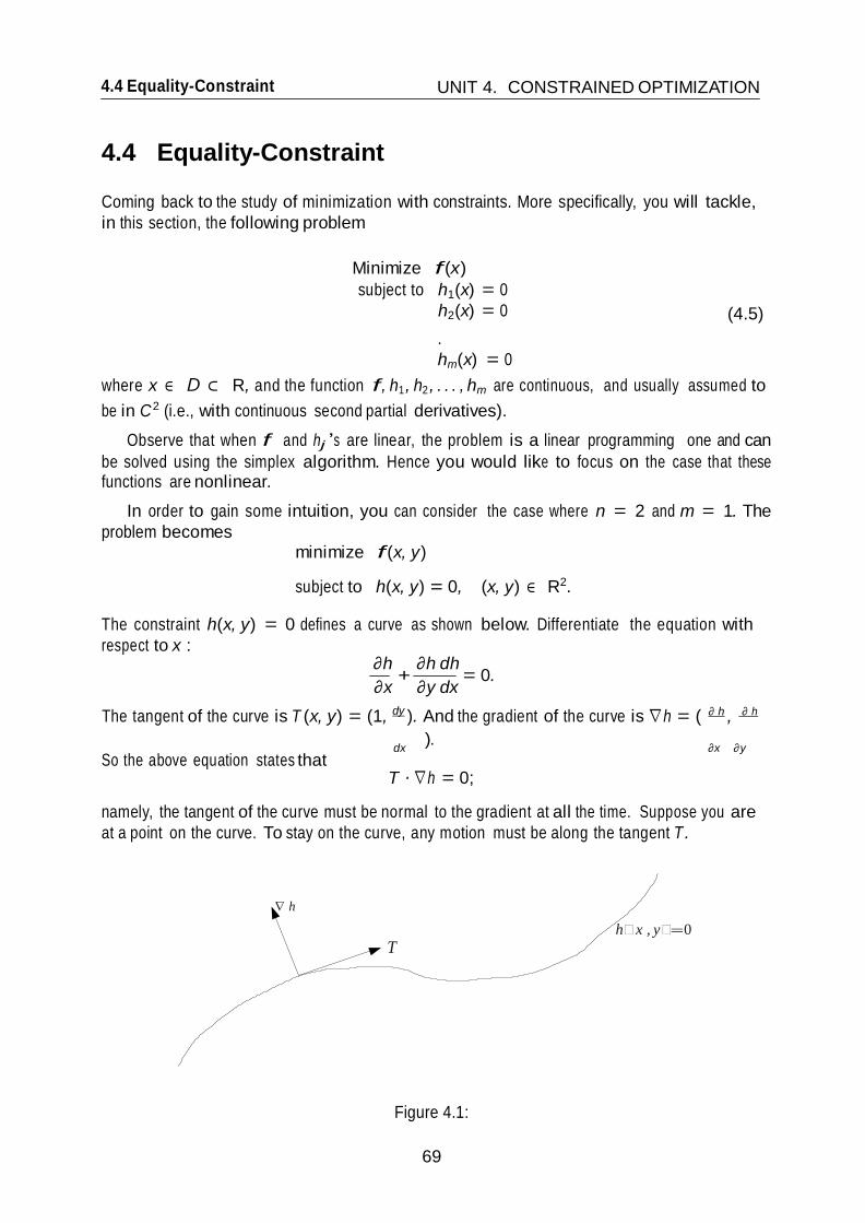
69
4.4 Equality-Constraint UNIT 4. CONSTRAINED OPTIMIZATION
4.4 Equality-Constraint
Coming back to the study of minimization with constraints. More specifically, you will tackle,
in this section, the following problem
Minimize f (x)
subject to h1(x) = 0
h2(x) = 0
.
hm(x) = 0
(4.5)
where x ∈ D ⊂ R, and the function f, h1 , h2 , . . . , hm are continuous, and usually assumed to
be in C 2 (i.e., with continuous second partial derivatives).
Observe that when f and hj ’s are linear, the problem is a linear programming one and can
be solved using the simplex algorithm. Hence you would like to focus on the case that these functions are nonlinear.
In order to gain some intuition, you can consider the case where n = 2 and m = 1. The
problem becomes minimize f (x, y)
subject to h(x, y) = 0, (x, y) ∈ R2.
The constraint h(x, y) = 0 defines a curve as shown below. Differentiate the equation with
respect to x : ∂h
+ ∂h dh
= 0. ∂x ∂y dx
The tangent of the curve is T (x, y) = (1, dy ). And the gradient of the curve is ∇h = ( ∂ h , ∂ h
).
So the above equation states that dx
T · ∇h = 0;
∂x ∂ y
namely, the tangent of the curve must be normal to the gradient at all the time. Suppose you are
at a point on the curve. To stay on the curve, any motion must be along the tangent T .
h
T
Figure 4.1:
h x , y 0
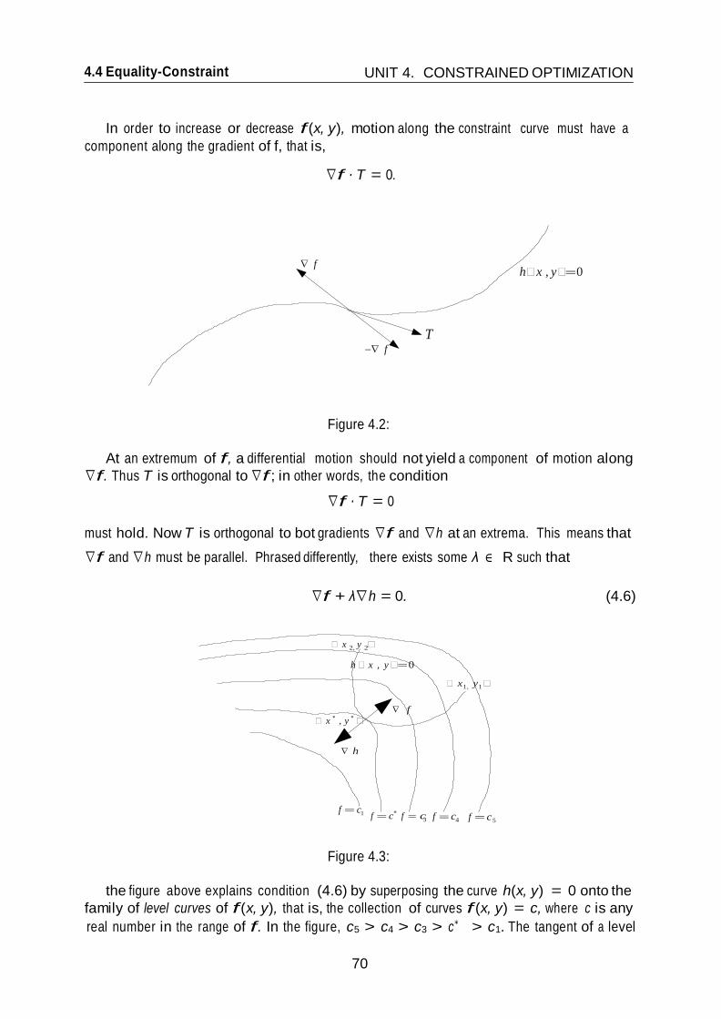
4.4 Equality-Constraint UNIT 4. CONSTRAINED OPTIMIZATION
70
3 4
In order to increase or decrease f (x, y), motion along the constraint curve must have a
component along the gradient of f, that is,
∇f · T = 0.
f h x , y 0
T f
Figure 4.2:
At an extremum of f, a differential motion should not yield a component of motion along
∇f. Thus T is orthogonal to ∇f ; in other words, the condition
∇f · T = 0
must hold. Now T is orthogonal to bot gradients ∇f and ∇h at an extrema. This means that
∇f and ∇h must be parallel. Phrased differently, there exists some λ ∈ R such that
∇f + λ∇h = 0. (4.6)
x 2, y 2
h x , y 0
f
x
, y
h
x1, y1
f c1 f c
f c f c
f c5
Figure 4.3:
the figure above explains condition (4.6) by superposing the curve h(x, y) = 0 onto the
family of level curves of f (x, y), that is, the collection of curves f (x, y) = c, where c is any
real number in the range of f. In the figure, c5 > c4 > c3 > c∗ > c1. The tangent of a level

4.4 Equality-Constraint UNIT 4. CONSTRAINED OPTIMIZATION
71
+ λ
∂y ∂ y
curve is always orthogonal to the gradient ∇f. Otherwise moving along the curve would result in an increase or decrease of the value of f. Imagine a point moving on the curve h(x, y) = 0
from (x1, y1) to (x2, y2). Initially, the motion has a component along the negative gradient direction − ∇f, resulting in the decrease of the value of f. This component becomes smaller
and smaller. When the moving point reaches (x ∗ , y ∗ ), the motion is orthogonal to the gradient. From that point on, the motion starts having a component along the gradient ∇f so the value of f increases. Thus at (x∗ , y ∗ ), f achieves its local minimum. The motion is in the tangential direction of the curve h(x, y) = 0, which is orthogonal to the gradient ∇h. Therefore at the point (x∗ , y∗ ) the two gradients ∇f and ∇h must be collinear. This is what equation (4.6) says. Let c∗ be the local minimum achieved at (x∗ , y∗ ). It is clear that the two curves f (x, y) = c∗ and h(x, y) = 0 are tangent at (x∗ , y∗ ).
Suppose you find the set S of points satisfying the equations
h(x, y) = 0
∇f + λ∇h = 0 for some λ
Then S contains the external points of f to the constraints h(x, y) = 0. The above two equa-
tions constitute a nonlinear system in the variables x, y, λ. It can be solved using numerical
techniques, for example, Newton’s method.
4.4.1 Lagrangian
It is convenient to introduce the Lagrangian associated with the constrained problem, defined
as
Note
F (x, y, λ) = f (x, y) + λh(x, y)
∂ f ∂ h T
∂x ∂ x
∇F = ∂ f + λ ∂ h = (∇f + λh, h).
h
Thus setting ∇F = 0 yields the same system of nonlinear equations you derived earlier.
The value λ is known as the Lagrange multiplier. The approach of constructing the La-
grangians and setting its gradient to zero is know as the method of Lagrange multipliers.
Example 4.4.1 Find the extremal values of f (x, y) = xy subject to the constraint
h(x, y) = x2 y2
+ 8 2
− 1 = 0
☞ Solution. First construct the Lagrangian and find its gradient:
( 2
F (x, y, λ) = xy + λ x y2
\ + − 1 ,
∇F (x, y, λ) =
8 2
y + λ x 4 x + λy = 0
x2 y 2
8 +
2 − 1

4.4 Equality-Constraint UNIT 4. CONSTRAINED OPTIMIZATION
72
The above leads to three equations
λx y + = 0, (4.7)
4 x + λy = 0, (4.8)
x2 + 4y2 = 8. (4.9)
combining (4.7) and (4.8) yields
λ2 = 4 and λ = ±2
Thus x = ±2y. Substituting this equation into (4.9) gives you
y = ±1 and x = ±2.
So there are four extremal points of f subject to the constraint h : (2, 1), (− 2, − 1), (2, − 1), and
(− 2, − 1). The maximum value 2 is achieved at the first two points while the minimum value − 2 is achieved at the last two points.
Figure 4.4:
Graphically, the constraint h defines an ellipse. The constraint contours of f are the hyper- bolas xy = c, with |c| increasing as the curves move out from the origin. ✍

4.4 Equality-Constraint UNIT 4. CONSTRAINED OPTIMIZATION
73
if
dt
h(x1, x2) = x 1
4.4.2 General Formulation Now you would generalize to the case with multiple constraints. Let h = (h1, . . . , hm)T be a
function from Rn to Rm. Consider the constrained optimization problem below.
minimize f (x)
subject to h(x) = 0
Each constraint equation hj (x) = 0 defines a constraint hypersurface S in the space Rn. And this surface is smooth provided hj (x) ∈ C 1.
A curve on S is a family of points x(t) ∈ S with a ≤ t ≤ b. The curve is dx(t) dx
differentiable
dt exists, and twice differentiable if
x∗ = x∗ (t) for some t∗ , a ≤ t∗ ≤ b.
dt2 exists. The curve passes through a point x∗ if
The tangent space at x∗ is the subspace of Rn spanned by the tangents dx (t∗ ) of all curves x(t) on S such that x(t∗ ) = x∗ . In other words, the tangent space is the set of the derivatives at x∗ of all surface curves through x∗ . Denote this subspace as T .
A point x satisfying h(x) = 0 is a regular point of the constraint if the gradient vectors
∇h1 (x), . . . , ∇hm (x) are linearly independent.
From your previous intuition, you would expect that ∇f · v = 0 for all v ∈ T at an
extremum. This implies that ∇f lies in the orthogonal complement T ⊥ of T . Claim that ∇f
can be composed from a linear combination of the ∇hi’s. This is only valid provided that these
gradients span T ⊥ , which is true when the extremal point is regular.
Theorem 4.4.1 At a regular point x of the surface S defined by h(x) = 0, the tangent space is
the same as
where the matrix
{y = |∇h(x)y = 0}
∇h1
∇ h = .
∇hm
The rows of the matrix ∇h(x) are the gradient vectors ∇hj (x), j = 1, . . . , m. The theo-
rem says that the tangent space at x is equal to the nullspace of ∇h(x). Thus its orthogonal
complement T ⊥ must equal the row space of ∇h(x). Hence the vectors ∇hj (x) span T ⊥ .
Example 4.4.2 Suppose h(x1, x2) = x1. Then h(x) = 0 yields the x2 axis. And ∇h = (1, 0) at all
points. So every x ∈ R2 is regular. The tangent space is also the x2 axis and has dimension 1. If instead 2, then h(x) = 0 still defines the x2 axis. On this ∇h = (2x1, 0) = (0, 0). Thus no
point is regular. The dimension of T , which is the x2 axis, is still one, but the dimension of the space
{y|∇h · y = 0} is two.
Lemma 4.4.1 Let x∗ be a local extremum of f subject to the constraints h(x) = 0. Then for all y in the tangent space of the constraint surface at x∗ ,
∇f (x∗ )y = 0.

4.4 Equality-Constraint UNIT 4. CONSTRAINED OPTIMIZATION
74
The next theorem states that the Lagrange multiplier method as a necessary condition on an
extremum point.
Theorem 4.4.2 (First-Order Necessary Conditions) Let x∗ be a local extremum point of f subject to the constraints h(x) = 0. Assume further that x∗ is a regular point of these con- straints. Then there is a λ ∈ Rn such that
∇f (x∗ ) + λT ∇h(x∗ ) = 0.
The first order necessary conditions together with the constraints
h(x∗ ) = 0
give a total of n + m equations in n + m variables x∗ and λ. Thus a unique solution can be
determined at least locally.
Example 4.4.3 You can construct a cardboard box of maximum volume, given a fixed area of card-
board.
Denoting the dimension of the box by x, y, z, the problem can be expressed a
maximize xyz c
subject to xy + yz + xz = 2 ,
where c > 0 is the given area of cardboard. Consider the Lagrangian xyz + λ(xy + yz + xz − c ). The 2
first-order necessary conditions are easily found to be
yz + λ(y + z) = 0, (4.10)
xz + λ(x + z) = 0, (4.11)
xy + λ(x + y) = 0. (4.12)
together with the original constraint. Before solving the equation above, note that their sum is
(xy + yz + xz) + 2λ(x + y + z) = 0,
which, given the constraint, becomes
c/2 + 2λ(x + y + z) = 0.
Hence it is clear that λ = 0. Neither of x, y, z can be zero since if either is zero, all must be so according
to (4.10)-(4.12).
To solve the equations (4.10)-(4.12), multiply (4.10) by x and (4.11) by y, and then subtract the two to
obtain
λ(x − y)z = 0
Operate similarly on the second and third to obtain
λ(y − z)x = 0.
Since no variables can be zero, it follows that
x = y = z = c 6
is the unique solution to the necessary conditions. The box must be a cube.

4.4 Equality-Constraint UNIT 4. CONSTRAINED OPTIMIZATION
75
1 2 3
You can derive the second-order conditions for constrained problems, assuming f and h are
twice continuously differentiable.
Theorem 4.4.3 (Second-Order Necessary Conditions) Suppose that x ∗ is a local minimum of f subject to h(x) = 0 and that x∗ is a regular point of these constraints. Then there is a λ ∈ Rm such that
The matrix
∇f (x∗ ) + λT ∇h(x∗ ) = 0.
m
L(x∗ ) = H f (x∗ )
+ i=1
λiH hi (x) (4.13)
is positive semidefinite on the tangent space {y|∇h(x∗ )y = 0}.
Theorem 4.4.4 (Second-Order Sufficient Conditions) Suppose there is a point x∗ satisfying
h(x∗ ) = 0, and a λ such that
∇f (x∗ ) + λT h(x∗ ) =
0.
Suppose also that the matrix L(x∗ ) defined in (4.13) is positive definite on the tangent space
{y|∇h(x∗ )y = 0}. Then x∗ is a strict local minimum of f subject to h(x) = 0.
Example 4.4.4 Consider the problem
minimize x1 x2 + x2 x3 + x1 x3
subject to x1 + x2 + x3 = 3
The first order necessary conditions become
x2 + x3 + λ = 0
x1 + x3 + λ = 0
x1 + x2 + λ = 0.
You can solve these equations together with the one constraint equation and obtain
x1 = x2 = x3 = 1 and λ = − 2
Thus x∗ = (1, 1, 1)T .
Now you need to resort to the second-order sufficient conditions to determine if the problem
achieves a local maximum and minimum at x1 = x2 = x3 = 1. You will find the matrix
L(x∗ ) = H f (x∗ ) + λH h(x∗
)
0 1 1
= 1 0 1
1 1 0
is neither positive nor negative definite. On the tangent space M = {y|y1 + y2 + y3 = 0},
however, you note that
yT Ly = y1(y2 + y3) + y2(y1 + y3) + y3(y1 + y2 )
= − (y2 + y2 + y2)
< 0, for all y = 0.
Thus L is negative definite on M and the solution 3 you found is atleas a local maximum.

76
4.5 Inequality Constraints UNIT 4. CONSTRAINED OPTIMIZATION
4.5 Inequality Constraints
Finally, you will address the problems of the general form
Minimize f (x)
subject to h(x) = 0
g(x) ≥ 0
where h = (h1, . . . , hm)T and g = (g1 , . . . , gp )T .
A fundamental concept that provides a great deal of insight as well as simplifies the required theoretical development is that of an active constraint. An inequality constraint gi(x) ≤ 0 is
said to be active at a feasible point x if gi (x) = 0 and inactive at x if gi(x) = 0. By convention
you refer to any equality constraint hi(x) = 0 as active at any feasible point. The constraints
active at a feasible point x restrict the domain of feasibility in neighbourhood of x. Therefore, in studying the properties of a local minimum point, it is clear that attention can be restricted to the active constraints. This is illustrated in the figure below where local properties satisfied by
the solution x∗ obviously do not depend on the inactive constraints g2 and g3 .
Assume that the function f , h = (h1, . . . , hm)T , g = (g1 , . . . , gp)T are twice continuously
differentiable. Let x∗ be a point satisfying the constraint.
h(x∗ ) = 0 and g(x∗ )
≤
0,
and let J = {j|gj (x∗ ) = 0}. Then x∗ is said to be a regular point of the above constraints if
the gradient vectors ∇hi (x∗ ), ∇gj (x
∗ ), 1 ≤ i ≤ m, j ∈ J are linearly independent.
Now suppose this regular point x∗ is also a relative minimum point for the original problem (4.6). Then it is shown that there exists a vector λ ∈ Rm and a vector µ ∈ Rp with µ ≥ 0 such that
∇f (x∗ ) + λT ∇h(x∗ ) + µT ∇g(x∗ ) =
0
µT g(x∗ ) = 0
Since µ ≥ 0 and g(x∗ ) ≤ 0, the second constraint above is equivalent to the statement
that
a component of µ may be nonzero only if the corresponding constraint is active. To find a solu- tion, you can enumerate various combinations of active constraints, that is, constraints where
equalities are attained at x∗ , and check the signs of the resulting Lagrangian multipliers.
There are a number of distinct theories concerning this problem, based on various regular-
ity conditions or constraint qualifications, which are directed toward obtaining definite general
statements of necessary and sufficient conditions. One can by no means pretend that all such re-
sults can be obtained as minor extensions of the theory for problems having equality constraints
only. To date, however, their use has been limited to small-scale programming problems of two
or three variables.

77
4.5 Inequality Constraints UNIT 4. CONSTRAINED OPTIMIZATION
4.6 Conclusion

78
4.5 Inequality Constraints UNIT 4. CONSTRAINED OPTIMIZATION
In this unit, you were introduced to constrained optimization problems, which could be equality,
inequality, or mixed constraints. You looked at the theorem of Lagrange for local optimum of a

79
4.7 Summary UNIT 4. CONSTRAINED OPTIMIZATION
constrained problem.
4.7 Summary
Having gone through this unit, you now
(i) define equality and inequality constrained optimization problem.
(ii) state and use the lagrange theorem.
(iii) State and apply the First-Order Necessary Conditions.
(iv) State and apply the second-order necessary and sufficient conditions.
4.8 Tutor Marked Assignments(TMAs)
Exercise 4.8.1
1. Find the minimum and maximum of f (x, y) = x2 − y2 on the unit circle x2 + y2 = 1
using the Lagrange multipliers method. Using the substitution y2 = 1 − x2, solve the
same problem as a single variable unconstrained proble. Do you get the same results? Why or Why not?
2. Show that the problem of maximizing f (x, y) = x3 + y3 on the constraint set D =
{(x, y)|x + y = 1} has no solution. Show also that if the Lagrangian method were used on this problem, the critical points of the Lagrangian have a unique solution. Is the point identified by this solution either a local maximum or a (local or global) minimum?
3. Find the maxima and minima of the following functions subject to the specified con-
straints:
(a) f (x, y) = xy subject to x2 + y2 = 2a2.
(b) f (x, y) = 1/x + 1/y subject to (1/x)2 + (1/y)2 = (1/a)2 .
(c) f (x, y, z) = x + y + z subject to (1/x) + (1/y) + (1/z) = 1.
(d) f (x, y, z) = xyz subject to x + y + z = 5 and xy + xz + yz = 8.
(e) f (x, y, z) = x + y for xy = 16
(f) f (x, y, z) = x2 + 2y − z2 subject to 2x − y = 0 and x + z = 6.
4. Maximize and minimize f (x, y) = x + y on the lemniscate (x2 − y2)2 = x2 + y2.
5. Consider the problem
min x2 + y2 subject to (x − 1)3 − y2 = 0.
(a) Solve the problem geometrically.

80
4.8 Tutor Marked Assignments(TMAs) UNIT 4. CONSTRAINED OPTIMIZATION
(b) Show that the method of Lagrange multipliers does not work in this case. Can you
explain why?
6. Consider the following problem where the objective function is quadratic and the con-
straints are linear
max cT x + 1
xT Dx subject to Ax = b x 2
where c is a given n-vector. D is a given n × n symmetric, negative definite matrix, and A is a given m × n matrix.
(a) Set up the Lagrangean and obtain the first-order condtions.
(b) Solve for the optimal vector x∗ as a function of A, b, c and D.
7. Solve the problem
max f (x) = xT Ax subject to x · x = 1
where A is a given symmetric matrix.
8. Solve the following maximization problem:
Maximize ln x + ln y
Subject to x2 + y2 = 1 with x, y ≥ 0.
References
1. Sundaram, R. K., A First Course In Optimization Theory, New York University, 1996.
2. Murtagh, B. A., Advanced Linear Programming, McGraw-Hill, New York, 1981.
3. Luenberger D. G. Introduction to Linear and Nonlinear Programming, Addison-Wesley,
Reading, Mass., 1973.
4. Rockafeller, R. T. Convex Analysis, Princeton University Press, Princeton N. J., 1970.
5. Djitte N., Lecture Notes on Optimization Theory in Rn, Gaston Berger University, Sene- gal., 2006.
6. Freund R. M., Introduction to Optimization, and Optimality Conditions for Unconstrained
Problems, MIT, 2004.