EPA/600/R-19/076

August 2019

NATIONAL STORMWATER CALCULATOR WEB APP USER’S GUIDE – VERSION 3.2.0

By

Lewis A. Rossman (retired) Water Systems Division

National Risk Management Research Laboratory Cincinnati, OH 45268

Jason T. Bernagros Water System Division

National Risk Management Research Laboratory Cincinnati, OH 45268

ii

OFFICE OF RESEARCH AND DEVELOPMENT U.S. ENVIRONMENTAL PROTECTION AGENCY

CINCINNATI, OH 45268

DISCLAIMER

The information in this document has been funded wholly by the U.S. Environmental Protection Agency (EPA). It has been subjected to the Agency’s peer and administrative review, and has been approved for publication as an EPA document. Mention of trade names or commercial products does not constitute endorsement or recommendation for use.

Although a reasonable effort has been made to assure that the results obtained are correct, the computer programs described in this manual are experimental. Therefore the author and the U.S. Environmental Protection Agency are not responsible and assume no liability whatsoever for any results or any use made of the results obtained from these programs, nor for any damages or litigation that result from the use of these programs for any purpose.

iii

ACKNOWLEDGEMENTS

Paul Duda, Paul Hummel, Jack Kittle, and John Imhoff of Aqua Terra Consultants developed the data acquisition portions of the National Stormwater Calculator desktop application under Work Assignments 4-38 and 5-38 of EPA Contract #EP-C-06-029. They, along with Alex Foraste (EPA/OW), provided many useful ideas and feedback throughout the development of the calculator. Scott Struck, Dan Pankani, and Kristen Ekeren of Geosyntec, and Marion Deerhake of RTI International developed the cost estimation components of the Stormwater Calculator under Task Orders 0019 (PR-ORD-14-00308) and 026 (PR-ORD-15-00668). Jason Bernagros served as the Task Order Contracting Officer’s Representative (TOCOR) for the cost estimation task order and the TOCOR for the mobile web application (a.k.a., app). Jason Bernagros served as the Work Assignment Manager for the maintenance of the mobile web app. Michael Tryby and Michelle Simon, in EPA’s Office of Research and Development (ORD), provided project guidance and valuable feedback throughout the development of the cost estimation procedures and the mobile web app. Dawn Bontempo, Fahim Chowdhury, Marie Calvo, Martina Donati, Jason Lowengrub, Anthony Passamonti, Seth Pennington, Catherine Sweeney, and Natasha Virdy of Attain, LLC., Uyen Tran of Tetra Tech, and developed the mobile web app version of the Stormwater Calculator under Task Order HHSN316201200117W (EP-G15H-01113). Colleen Barr, was supported in part by an appointment to the Postdoctoral Research Program at the U.S. Environmental Protection Agency, Office of Research and Development, National Risk Management Research Laboratory, administered by the Oak Ridge Institute for Science and Education through Interagency Agreement No. (DW-8992433001) between the U.S. Department of Energy and the U.S. Environmental Protection Agency, and provided programming support for the maintenance of the mobile web application. Brad Cooper, Mike Liadov, and Naveen Tharalla of Eastern Research Group (ERG) (under Work Assignment 0-52 (EP-C-17-041) also provided some programming support for the mobile application for the Stormwater Calculator.

iv

ACRONYMS AND ABBREVIATIONS

ASCE = American Society of Civil Engineers BLS = United States Bureau of Labor Statistics CMIP3 = Coupled Model Intercomparison Project Phase 3 CREAT = Climate Resilience Evaluation and Awareness Tool EPA = United States Environmental Protection Agency GCM = General Circulation Model GEV = Generalized Extreme Value GI = Green Infrastructure HSG = Hydrologic Soil Group IMD = initial moisture deficit IPCC = Intergovernmental Panel on Climate Change Ksat = saturated hydraulic conductivity LID = low impact development NCDC = National Climatic Data Center NRCS = Natural Resources Conservation Service NWS = National Weather Service OW = Office of Water SCS = Soil Conservation Service SSURGO = Soil Survey Geographic Database SWAT = Soil and Water Assessment Tool SWC = Stormwater Calculator SWMM = Storm Water Management Model UDFCD = Urban Drainage and Flood Control District US = United States USDA = United States Department of Agriculture WCRP = World Climate Research Programme

v

TABLE OF CONTENTS DISCLAIMER................................................................................................................................................... ii

ACKNOWLEDGEMENTS ................................................................................................................................ iii

ACRONYMS AND ABBREVIATIONS ............................................................................................................... iv

TABLE OF CONTENTS ..................................................................................................................................... v

LIST OF FIGURES ........................................................................................................................................... vi

List of Tables .............................................................................................................................................. viii

1. Introduction .............................................................................................................................................. 9

2. How to Run the Calculator ...................................................................................................................... 11

Location ................................................................................................................................................... 12

Soil Type .................................................................................................................................................. 16

Soil Drainage ........................................................................................................................................... 18

Topography ............................................................................................................................................. 19

Precipitation/Evaporation ....................................................................................................................... 20

Climate Change ....................................................................................................................................... 23

Land Cover .............................................................................................................................................. 25

LID Controls (including cost estimation options) .................................................................................... 27

Results ..................................................................................................................................................... 32

3. Interpreting the Calculator’s Results ...................................................................................................... 35

Summary Results..................................................................................................................................... 35

Rainfall / Runoff Events ........................................................................................................................... 37

Rainfall / Runoff Frequency .................................................................................................................... 38

Rainfall Retention Frequency .................................................................................................................. 39

Runoff by Rainfall Percentile ................................................................................................................... 41

Extreme Event Rainfall/Runoff ............................................................................................................... 42

Cost Summary ......................................................................................................................................... 44

Printing Output Results ........................................................................................................................... 48

4. Applying LID Controls .............................................................................................................................. 49

vi

5. Example Application ............................................................................................................................... 53

Pre-Development Conditions .................................................................................................................. 53

Post-Development Conditions ................................................................................................................ 57

Post-Development with LID Practices ..................................................................................................... 59

Cost Summary ......................................................................................................................................... 65

Climate Change Impacts ......................................................................................................................... 69

6. Computational Methods ......................................................................................................................... 75

SWMM’s Runoff Model .......................................................................................................................... 75

SWMM’s LID Model ................................................................................................................................ 76

Site Model without LID Controls ............................................................................................................. 78

Site Model with LID Controls .................................................................................................................. 81

Precipitation Data ................................................................................................................................... 82

Evaporation Data .................................................................................................................................... 85

Climate Change Effects ........................................................................................................................... 86

Cost Estimation ....................................................................................................................................... 89

Post-Processing ..................................................................................................................................... 102

7. References ............................................................................................................................................ 104

LIST OF FIGURES

Figure 1. The calculator's (a) opening page and (b) Location icon page. .................................................... 11 Figure 2. The calculator’s Location icon page. ............................................................................................ 13 Figure 3. Bird’s eye map view with a bounding circle. ................................................................................ 14 Figure 4. Bird’s eye map view with a bounding polygon. ........................................................................... 15 Figure 5. The calculator’s Soil Type page. ................................................................................................... 17 Figure 6. The calculator's Soil Drainage icon page. ..................................................................................... 19 Figure 7. The calculator's Topography icon page. ...................................................................................... 20 Figure 8. The calculator's Precipitation/Evaporation icon page. ................................................................ 21 Figure 9. The calculator's Precipitation/Evaporation icon page (weather station). ................................... 22 Figure 10. The calculator's Climate Change icon page. .............................................................................. 24 Figure 11. The calculator's Land Cover page. ............................................................................................. 26 Figure 12. The calculator’s LID Controls icon page. .................................................................................... 28 Figure 13. The Calculator’s Project Cost icon page showing the Re-Development pop-out window (shown by clicking Re-Development) ....................................................................................................................... 29

vii

Figure 14. The Calculator’s Project Cost icon page showing the Site Suitability - Poor pop-out window (shown by clicking Poor). ............................................................................................................................ 30 Figure 15. Map of BLS Regional Cost Centers (pop-out window) used for computing regional multipliers. A multiplier for each Regional Center applied within a 100-mile radius (inside blue circles). A National value of 1 used otherwise (in green areas). ................................................................................................ 31 Figure 16. Drop down list of closest BLS Regional Cost Centers and national value. ................................. 32 Figure 17. The calculator’s Results page icon. ............................................................................................ 33 Figure 18. An example of the calculator’s Summary Results report. ......................................................... 36 Figure 19. The calculator's Rainfall / Runoff Event report. ......................................................................... 38 Figure 20. The calculator’s Rainfall / Runoff Frequency report. ................................................................. 39 Figure 21. The calculator’s Rainfall Retention Frequency report. .............................................................. 40 Figure 22. The calculator’s Runoff by Rainfall Percentile report. ............................................................... 41 Figure 23. The calculator’s Extreme Event Rainfall / Runoff report. .......................................................... 43 Figure 24. Graphical output option of the calculator's estimate of average capital costs. ........................ 46 Figure 25. Graphical output option of the calculator's estimate of average annual maintenance costs. .. 48 Figure 26. Example of an LID Design dialog for a street planter. ................................................................ 51 Figure 27. Pre-development conditions land cover. ................................................................................... 54 Figure 28. Runoff from different size storms for pre-development conditions on the example site. ....... 56 Figure 29. Rainfall retention frequency under pre-development conditions for the example site. .......... 57 Figure 30. Rainfall retention frequency for pre-development (Baseline) and post-development (Current) conditions.................................................................................................................................................... 59 Figure 31. Low Impact Development controls applied to the example site. .............................................. 60 Figure 32. Design parameters for Rain Harvesting and Rain Garden controls. .......................................... 61 Figure 33. Design parameters for the Infiltration Basin and Permeable Pavement controls ..................... 62 Figure 34. Daily runoff frequency curves for pre-development (Baseline) and post-development with LID controls (Current) conditions. ..................................................................................................................... 64 Figure 35. Contribution to total runoff by different magnitude storms for pre-development (Baseline) and post-development with LID controls (Current) conditions. ................................................................. 64 Figure 36. Retention frequency plots under pre-development (Baseline) and post-development with LID controls (Current) conditions. ..................................................................................................................... 65 Figure 37. Graphical output option of the calculator's estimate of capital costs. ...................................... 67 Figure 38. Graphical output option of the calculator's estimate of maintenance costs. ........................... 69 Figure 39. Climate change scenarios for the example site. ........................................................................ 70 Figure 40. Daily rainfall and runoff frequencies for the historical (Baseline) and Warm/Wet climate scenarios. .................................................................................................................................................... 72 Figure 41. Target event retention for the historical (Baseline) and Warm/Wet climate scenarios. .......... 73 Figure 42. Extreme event rainfall and runoff for the Warm/Wet climate change scenario and the historical record (Baseline). ........................................................................................................................ 74 Figure 43. Conceptual representation of a bio-retention cell. ................................................................... 76 Figure 44. NWS rain gage locations included in the calculator. ................................................................. 83 Figure 45. NRCS (SCS) 24-hour rainfall distributions (USDA, 1986). ........................................................... 84 Figure 46. Geographic boundaries for the different NRCS (SCS) rainfall distributions (USDA, 1986). ....... 84

viii

Figure 47. Locations with computed evaporation rates (Alaska and Hawaii not shown). ......................... 85 Figure 48. CMIP3 2060 projected changes in temperature and precipitation for Omaha, NE (EPA, 2012). .................................................................................................................................................................... 87 Figure 49. Conceptual overview of cost estimate ranges derived from cost curves. ................................. 98 Figure 50. Sample regression cost curve for Rain Gardens. ....................................................................... 99

List of Tables

Table 1. Definitions of Hydrologic Soil Groups (USDA, 2010). .................................................................... 18 Table 2. Tabular representation of the calculator's estimate of capital costs. .......................................... 45 Table 3. Tabular output option of the calculator's estimate of annual maintenance costs. ...................... 47 Table 4. Descriptions of LID practices included in the calculator. .............................................................. 50 Table 5. Editable LID parameters. ............................................................................................................... 52 Table 6. Void space values of LID media. .................................................................................................... 52 Table 7. Summary results for pre-development conditions on the example site. ..................................... 55 Table 8. Land cover for the example site in developed state. .................................................................... 57 Table 9. Comparison of runoff statistics for post-development (Current) and pre-development (Baseline) conditions.................................................................................................................................................... 58 Table 10. Runoff statistics for pre-development (Baseline) and post-development with LID controls (Current) scenarios...................................................................................................................................... 63 Table 11. Tabular output option of the calculator's estimate of capital costs. .......................................... 66 Table 12. Tabular output option of the calculator's estimate of maintenance costs. ................................ 68 Table 13. Summary results under a Warm/Wet (Current) climate change scenario compared to the historical (Baseline) condition..................................................................................................................... 71 Table 14. Depression storage depths (inches) for different land covers. ................................................... 79 Table 15. Roughness coefficients for different land covers. ....................................................................... 80 Table 16. Infiltration parameters for different soil types. .......................................................................... 81 Table 17. Cost Variables Selected for Cost Estimation Procedure .............................................................. 90 Table 18. LID Control Cost Curve Regression Equations ............................................................................. 92 Table 19. Project Complexity Computation Based on User Input .............................................................. 93 Table 20. Regionalized Cost Model Coefficients for BLS Center ................................................................. 96 Table 21. BLS Regional Centers ................................................................................................................. 100 Table 22. National BLS Variables and Model Coefficients ........................................................................ 101

9

1. Introduction

The National Stormwater Calculator (https://www.epa.gov/water-research/national-stormwater-calculator) is a simple to use tool for computing small site hydrology for any location within the US. It estimates the amount of stormwater runoff generated from a site under different development and control scenarios over a long-term period of historical rainfall. The analysis takes into account local soil conditions, slope, land cover, and meteorology. Different types of low impact development (LID) practices (also known as green infrastructure) can be employed to help capture and retain rainfall on-site. Future climate change scenarios taken from internationally recognized climate change projections can also be considered. The calculator provides planning level estimates of capital and maintenance costs which will allow planners and managers to evaluate and compare effectiveness and costs of LID controls.

The calculator’s primary focus is informing site developers and property owners on how well they can meet a desired stormwater retention target. It can be used to answer such questions as the following:

• What is the largest daily rainfall amount that can be captured by a site in either its pre-development, current, or post-development condition?

• To what degree will storms of different magnitudes be captured on site? • What mix of LID controls can be deployed to meet a given stormwater retention target? • How well will LID controls perform under future meteorological projections made by global

climate change models? • What are the relative cost (capital and maintenance) differences for various mixes of LID

controls?

The calculator seamlessly accesses several national databases to provide local soil and meteorological data for a site. The user supplies land cover information that reflects the state of development they wish to analyze and selects a mix of LID controls to be applied. After this information is provided, the site’s hydrologic response to a long-term record of historical hourly precipitation, possibly modified by a particular climate change scenario, is computed. This allows a full range of meteorological conditions to be analyzed, rather than just a single design storm event. The resulting time series of rainfall and runoff are aggregated into daily amounts that are then used to report various runoff and retention statistics. In addition, the site’s response to extreme rainfall events of different return periods is also analyzed.

The calculator uses the EPA Storm Water Management Model (SWMM) as its computational engine (https://www.epa.gov/water-research/storm-water-management-model-swmm). SWMM is a well-established, EPA developed model that has seen continuous use and periodic updates for 40 years. Its hydrology component uses physically meaningful parameters making it especially well-suited for application on a nation-wide scale. SWMM is set up and run in the background without requiring any involvement of the user.

10

The calculator is most appropriate for performing screening level analysis of small footprint sites up to 12 acres in size with uniform soil conditions. The hydrological processes simulated by the calculator include evaporation of rainfall captured on vegetative surfaces or in surface depressions, infiltration losses into the soil, and overland surface flow. No attempt is made to further account for the fate of infiltrated water that might eventually transpire through vegetation or re-emerge as surface water in drainage channels or streams.

The remaining sections of this guide discuss how to install the calculator, how to run it, and how to interpret its output. An example application is presented showing how the calculator can be used to analyze questions related to stormwater runoff, retention, and control. Finally, a technical description is given of how the calculator performs its computations and where it obtains the parameters needed to do so.

11

2. How to Run the Calculator

The National Stormwater Calculator mobile web app is an HTML5, platform neutral and responsive mobile version of the desktop version of the calculator. The mobile version supports the existing functionality of the desktop version of the calculator. It may be used with publicly available internet browsers on laptop and desktop computers, smartphones, and tablets—you must have an internet connection to run the calculator. The mobile web app functions best on the following web browsers: Google Chrome, Microsoft Edge, Apple Safari, and Mozilla Firefox. The mobile web app may be accessed from the following web page: https://swcweb.epa.gov/stormwatercalculator. The opening and main windows of the calculator are displayed in Figure 1. The main window uses a series of tabbed pages to collect information about the site being analyzed and to run and view hydrologic results. A Bing Maps display allows you to view the site’s location, its topography, selected soil properties and the locations of nearby rain gages and weather stations.

Figure 1. The calculator's (a) opening page and (b) Location icon page.

12

The various pages of the calculator are represented by icons and used as follows: 1. Location icon - establishes the site’s location 2. Soil Type icon - identifies the site’s soil type 3. Soil Drainage icon - specifies how quickly the site’s soil drains 4. Topography icon - characterizes the site’s surface topography 5. Precipitation/Evaporation icon - selects a nearby rain gage to supply hourly rainfall data and a

nearby weather station to supply evaporation rates 6. Climate Change icon – selects a climate change scenario to apply 7. Land Cover icon - specifies the site’s land cover for the scenario being analyzed 8. LID Controls icon - selects a set of LID control options, along with their design features, to

deploy within the site and specifies site and project considerations for cost estimation purposes 9. Project Costs icon - specifies site and project considerations for cost estimation purposes 10. Results icon - runs a long term hydrologic analysis and displays the results including estimates of

capital and average annual maintenance costs.

Six command options shown along the top of the web app can also be selected at any time:

1. U.S. EPA logo: This command takes you back to the homepage of the web app.

2. New: This command will discard all previously entered data and take you to the Location page where you can begin selecting a new site to analyze. You will first be prompted to save the data you entered for the current site.

3. Save: This command is used to save the information you have entered for the current site to a disk file. This file can then be re-opened in a future session of the calculator by selecting the Open command.

4. Open: This command allows you to open a previously saved site.

5. Resources: This command will show you helpful resources, such as the User’s Manual, general LID and green infrastructure information from the U.S. EPA, fact sheet, and climate change.

6. Contact: This command provides the SWC@epa.gov email address

You can move back and forth between the calculator’s icon pages to modify your selections. Most of the pages have a Help command that will display additional information about the page when selected. Text displayed as blue on the interface can generally be clicked to display more information. After an analysis has been completed on the Results icon page, you can choose to designate it as a “baseline” scenario, which means that its results will be displayed side-by-side with those of any additional scenarios that you choose to analyze. Each of the calculator’s icon pages will now be described in more detail.

Location The Location icon page of the calculator is shown in Figure 2. You are asked to identify where in the U.S. the site is located. This information is used to access national soils and meteorological databases as well as Bureau of Labor Statistics (BLS) data for cost estimation purposes. It has an address lookup feature that allows you to easily navigate to the site’s location. You can enter an address or zip code in the Search box and either click on the Search icon, or press the Enter key to move the map view to that

13

location. You can also use the map’s pan and zoom controls to hone in on a particular area. Once the site has been located somewhere within the map’s viewport, move the mouse pointer over the site and then left-click the mouse to mark its exact location with a drop-down point.

Figure 2. The calculator’s Location icon page.

The map display can be toggled between a standard road, aerial, bird’s eye, and streetside views. Figure 3 shows the site located in Figure 2 with a zoomed-in aerial view selected with the site bounded by an orange circle. You can specify the area of the site, which will result in a bounding orange circle or a polygon being drawn on the map. Figure 4 illustrates how a user may click on the polygon draw tool to draw out polygon points that create a connected polygon boundary around the project site. The project area cannot be larger than 12 acres. Entering the size of your site is optional because the calculator makes all of its computations on a per unit area basis.

You can also click on Open a previously saved site to read in data for a site that was previously saved to a file to continue working with those data (every time you begin analyzing a new site or exit the program the calculator asks if you want to save the current site to a file). Once you open a previously saved site, the calculator will be populated with its data.

14

Figure 3. Bird’s eye map view with a bounding circle.

15

Figure 4. Bird’s eye map view with a bounding polygon.

16

Soil Type

Figure 5 shows the Soil Type icon page of the calculator, which is used to identify the type of soil present on the site. Soil type is represented by its Hydrologic Soil Group (HSG). This is a classification used by soil scientists to characterize the physical nature and runoff potential of a soil. The calculator uses a site's soil group to infer its infiltration properties (Table 1).

You can select a soil type based on local knowledge or by retrieving a soil map overlay from the U.S. Department of Agriculture’s Natural Resources Conservation Service (NRCS) SSURGO database (https://websoilsurvey.sc.egov.usda.gov/App/HomePage.htm). Simply select the soil type icon on the left side of the screen to retrieve SSURGO data. (There will be a slight delay the first time that the soil data are retrieved and the color-coded overlay is drawn). There is an option to hide the soil polygon data under the soil type menu box. Figure 5 displays the results from a SSURGO retrieval. You can then select a soil type directly from the left panel or click on a color shaded region of the map.

17

Figure 5. The calculator’s Soil Type page.

The SSURGO database houses soil characterization data for most of the U.S. that have been collected over the past forty years by federal, state, and local agencies participating in the National Cooperative Soil Survey. These data are compiled by “map units” which are the boundaries that define a particular recorded soil survey. These form the irregular shaped polygon areas that are displayed in the calculator’s map pane.

Soil survey data do not exist for all parts of the country, particularly in downtown core urban areas; therefore, it is possible that no data will be available for your site. In this case you will have to rely on local knowledge to designate a representative soil group.

18

Table 1. Definitions of Hydrologic Soil Groups (USDA, 2010).

Group Meaning

Saturated Hydraulic

Conductivity (in./hr.)

A Low runoff potential. Soils having high infiltration rates even when thoroughly wetted and consisting chiefly of deep, well to excessively drained sands or gravels.

≥ 0.45

B Soils having moderate infiltration rates when thoroughly wetted and consisting chiefly of moderately deep to deep, moderately well to well-drained soils with moderately fine to moderately coarse textures. E.g., shallow loess, sandy loam.

0.30 - 0.15

C Soils having slow infiltration rates when thoroughly wetted and consisting chiefly of soils with a layer that impedes downward movement of water, or soils with moderately fine to fine textures. E.g., clay loams, shallow sandy loam.

0.15 - 0.05

D High runoff potential. Soils having very slow infiltration rates when thoroughly wetted and consisting chiefly of clay soils with a high swelling potential, soils with a permanent high water table, soils with a clay-pan or clay layer at or near the surface, and shallow soils over nearly impervious material.

0.05 - 0.00

Soil Drainage The Soil Drainage icon page of the calculator (Figure 6) is used to identify how fast standing water drains into the soil. This rate, known as the “saturated hydraulic conductivity,” is arguably the most significant parameter in determining how much rainfall can be infiltrated.

19

Figure 6. The calculator's Soil Drainage icon page.

There are several options available for assigning a hydraulic conductivity value (in inches per hour) to the site:

a) The edit box can be left blank, in which case, a default value based on the site’s soil type will beused (the default value is shown next to the edit box).

b) As with soil group, conductivity values from the SSURGO database are displayed on the mapwhen the soil drainage icon is selected. Clicking the mouse on a colored region of the map willmake its conductivity value appear in the edit box.

c) If you have local knowledge of the site’s soil conductivity you can simply enter it directly into theedit box. This is preferred over the other two choices.

It should be noted that the hydraulic conductivity values from the SSURGO database are derived from soil texture and depth to groundwater and are not field measurements. As with soil type, there may not be any soil conductivity data available for your particular location.

Topography

Figure 7 displays the Topography icon page of the calculator. Site topography, as measured by surface slope (feet of drop per 100 feet of length), affects how fast excess stormwater runs off a site. Flatter slopes results in slower runoff rates and provide more time for rainfall to infiltrate into the soil. Runoff rates are less sensitive to moderate variations in slope. Therefore, the calculator uses only four categories of slope – flat (2%), moderately flat (5%), moderately steep (10%) and steep (above 15%). As

20

with soil type and soil drainage, any available SSURGO slope data will be displayed on the map when the topography icon is selected. You can use the resulting display as a guide or use local knowledge to describe the site’s topography.

Figure 7. The calculator's Topography icon page.

Precipitation/Evaporation The Precipitation/Evaporation icon page of the calculator is shown in Figure 8. It is used to the select rain gage location that will supply rainfall data for the site and a National Weather Service Station as a source for evaporation rates. Rainfall is the principal driving force that produces runoff. The calculator uses a long term continuous hourly rainfall record to make sure that it can replicate the full scope of storm events that might occur. In addition, it identifies a set of 24-hour extreme event storms associated with each rain gage location. These are a set of six intense storms whose sizes are exceeded only once every 5, 10, 15, 30, 50 and 100 years, respectively.

21

Figure 8. The calculator's Precipitation/Evaporation icon page.

The calculator contains a catalog of over 8,000 rain gage locations from the National Weather Service’s (NWS) National Climatic Data Center (NCDC). Historical hourly rainfall data for each station have been extracted from the NCDC’s repository, screened for quality assurance, and stored on an EPA file server. As shown in Figure 8, the calculator will automatically locate the five nearest gages to the site and list their location, period of record and average annual rainfall amount. You can choose what you consider to be the most appropriate source of rainfall data for the site by selecting one of the available rain gages in the drop-down list or the map icons.

The Precipitation/Evaporation icon page of the calculator, also allows the user to select a weather station that will supply evaporation rates for the site. Evaporation determines how quickly the moisture retention capacity of surfaces and depression storage consumed during one storm event will be restored before the next event.

22

Figure 9. The calculator's Precipitation/Evaporation icon page (weather station).

Over 5,000 NWS weather station locations throughout the U.S. have had their daily temperature records analyzed to produce estimates of monthly average evaporation rates (i.e., twelve values for each station). These rates have been stored directly into the calculator. The calculator lists the five closest locations that appear in the table along with their period of record and average daily evaporation rate (the average of the twelve monthly rates). Note that these are “potential” evaporation rates, not recorded values (there are only a few hundred stations across the U.S. with long term recorded evaporation data). The rates have been estimated for bare soil using the Penman-Monteith equation; and thus, transpiration or vegetative land cover is not explicitly represented. More details are provided in the Computational Methods section of this document.

If the Download rainfall/evaporation data … command label is clicked, a Save As dialog window will appear allowing you to save the rainfall data to a text file in case you want to use those data in some other application, such as SWMM. Each line of the file will contain the recording station identification number, year, month, day, hour, and minute of the rainfall reading and the measured hourly rainfall intensity in inches/hour. If this option is selected, data will be written to a plain text file of your choice with the twelve monthly average rates appearing on a single line.

23

Climate Change The 2007 Fourth Assessment Report of the Intergovernmental Panel on Climate Change (IPCC) states that changing of the climate is now unequivocal (IPCC, 2007). Some of the impacts that such changes can have on the small-scale hydrology addressed by the calculator include changes in seasonal precipitation levels, more frequent occurrence of high intensity storm events, and changes in evaporation rates (Karl et al., 2009). A climate change component has been included in the calculator to help you explore how these impacts may affect the amount of stormwater runoff produced by a site and how it is managed.

Figure 10 displays the Climate Change icon page of the calculator. It is used to select a particular future climate change scenario for the site. The scenarios were derived from a range of outcomes of the World Climate Research Program’s CMIP3 multi-model dataset (Meehl et al., 2007). This dataset contains results of different global climate models run with future projections of population growth, economic activity, and greenhouse gas emissions. The results have been downscaled to a regional grid that encompasses each of the calculator’s rain gage and weather station locations. Three different scenarios are available that span the range of changes projected by the climate models: one is representative of model outputs that produce hot/dry conditions, another represents changes that come close to the median outcome from the different models, and a third represents model outcomes that produce warm/wet conditions. Projections for each scenario are available for two different future time periods: 2035 and 2060.

24

Figure 10. The calculator's Climate Change icon page.

Each choice of climate change scenario and projection year produces a different percent change in monthly average rainfall, monthly average temperature, and annual maximum day precipitation for each rain gage location and weather station in the calculator’s database. The precipitation changes for the current choice of rain gage are shown in the right hand panel of the Climate Change page. These changes are used to adjust the historical meteorological records for the site as follows:

1. The changes in monthly average rainfall are applied as a multiplier to each historical hourly rainfallreading that occurred in the particular month for each year of record.

2. The changes in monthly average temperatures are applied in similar fashion to the historical dailytemperature records used to calculate an average daily evaporation rate for each month of the year.

3. The climate change influenced extreme event rainfalls are used in place of the historical ones.

The hot/dry, median, and warm/wet scenarios can be used to better understand the uncertainty associated with future climate projections. For example, analyzing the two scenarios resulting in the most severe increases and decreases in rainfall respectively, brackets the range of possible rainfall conditions likely to occur. Alternately, if multiple scenarios are predicting increases in projected rainfall it is more likely that larger rainfall events will occur. All three scenarios should be considered when

25

bracketing future conditions, because the greatest projected change is not always associated with the hot/dry or warm/wet scenarios and is different from one location to the next.

More details on the source of the climate change scenarios and how they are used to compute site runoff are provided in the Computational Methods section of this user’s guide.

Land Cover

Understanding regional climate impacts may help you select appropriate climate change scenarios. Online resources highlighting regional climate change impacts for the contiguous U.S., Hawaii, Alaska, and U.S. Territories are available at (https://nca2018.globalchange.gov/ (USGRP, 2018) and at http://www.globalchange.gov/explore/ (USGRP, 2014)).

Figure 11 displays the Land Cover icon page of the calculator. It is used to describe the different types of pervious land cover on the site. Infiltration of rainfall into the soil can only occur through pervious surfaces. Different types of pervious surfaces capture different amounts of rainfall on vegetation or in natural depressions, and have different surface roughness. Rougher surfaces slow down runoff flow providing more opportunity for infiltration. The remaining non-pervious site area is considered to be “directly connected impervious surfaces” (roofs, sidewalks, streets, parking lots, etc. that drain directly off-site). Disconnecting some of this area, to run onto lawns for example, is an LID option appearing on the next page of the calculator. You are asked to supply the percentage of the site covered by each of four different types of pervious surfaces:

26

Figure 11. The calculator's Land Cover page.

You are asked to supply the percentage of the site covered by each of four different types of pervious surfaces:

1. Forest – stands of trees with adequate brush and forested litter cover2. Meadow – non-forested natural areas, scrub and shrub rural vegetation3. Lawn – sod lawn, grass, and landscaped vegetation4. Desert – undeveloped land in arid regions with saltbush, mesquite, and cactus vegetation

27

You should assign land cover categories to the site that reflects the specific condition you wish to analyze: pre-development, current, or post-development. A pre-development land cover will most likely contain some mix of forest, meadow, and perhaps desert. Local stormwater regulations might provide guidance on how to select a pre-development land cover or you could use a nearby undeveloped area as an example. Viewing the site map in bird’s eye view, as shown in Figure 11, would help identify the land cover for current conditions. Post-development land cover could be determined from a project’s site development plan map. Keep in mind that total runoff volume is highly dependent on the amount of impervious area on the site while it is less sensitive to how the non-impervious area is divided between the different land cover categories.

LID Controls (including cost estimation options) The LID Controls icon page of the calculator is depicted in Figure 12. It is used to deploy low impact development (LID) controls throughout the site. These are landscaping practices designed to capture and retain stormwater generated from impervious surfaces that would otherwise run off the site. There are seven different types of green infrastructure (GI) LID controls available (Figure 12). You can elect to apply any mix of these LID controls by simply telling the calculator what percentage of the impervious area is treated by each type of control. Each control has been assigned a reasonable set of design parameters, but these can be modified by clicking on the name of the control. You have the option to specify a 24-hour design storm to assist you with sizing the selected LID controls. More details on each type of control practice, its design parameters and sizing it to retain a given design storm are provided in the LID Controls section of this user’s guide. For the purposes of cost estimation, the calculator factors in the cost implications of construction feasibility and site suitability, and adjusts the cost of the LID Controls based on regional cost differences associated with a site’s location. Refer to the Cost Estimation section of this user guide (page 89) for a brief discussion of the cost curve approach used to generate estimates of probable capital and maintenance costs in the calculator. By indicating whether the project is new- or re-development and selecting from poor, moderate, or excellent for site suitability for placing LID controls along with other user input information, the calculator computes and applies the appropriate cost curve for the project.

For additional help with selecting the options that influence project site complexity, click the blue underlined text labeled Re-Development, New Development, Poor, Moderate, and Excellent on the LID controls tab, to show a help window explaining the conditions that warrant the selection of each of those options. An example of the help window for Re-Development is shown in Figure 13 and the help window for Poor (Site Suitability – Poor) is show in Figure 14.

The calculator uses Bureau of Labor Statistics (BLS) data to compute regional cost adjustment factors and allows the user to choose from the various computed factors as follows:

• National – this is the default selected value if your site is more than 100 miles from any of the 17BLS Regional Centers distributed across the country (including centers from the Northeast,Midwest, South, and West)

• Nearest 3 BLS Regional Centers – arranged in ascending order of distance from your project site.You have the option of selecting one of the nearest three BLS Regional Centers.

28

• Other – select this if you are an advanced user and want to specify your own regional costadjustment factor

Click on Cost Region for a map of the BLS Regional Centers (Figure 15). Regional cost multipliers for each Region are selected as the default multiplier for areas within a 100-mile radius of the regional center (see light blue circles in Figure 15). Areas that are not within a 100-mile radius of any regional center are assigned a default National value of 1 (see green areas in Figure 15). The user can override the default selection by selecting one of the three closest regions to their location from the Cost Region drop down menu (Figure 16). Note that regional cost multipliers that are greater than 1 increase costs, while multipliers that are less than 1 decrease costs compared to the National average. Additional information about the cost estimation procedure, including the BLS regional centers is provided on page 89.

Figure 12. The calculator’s LID Controls icon page.

29

Figure 13. The Calculator’s Project Cost icon page showing the Re-Development pop-out window (shown by clicking Re-Development)

30

Figure 14. The Calculator’s Project Cost icon page showing the Site Suitability - Poor pop-out window (shown by clicking Poor).

31

Figure 15. Map of BLS Regional Cost Centers (pop-out window) used for computing regional multipliers. A multiplier for each Regional Center applied within a 100-mile radius (inside blue circles).

A National value of 1 used otherwise (in green areas).

Green infrastructure (GI), similar to LID controls, is a relatively new and flexible term, and it has been used differently in different contexts. However, for the purposes of EPA's efforts to implement the GI Statement of Intent, EPA intends the term GI to generally refer to systems and practices that use or mimic natural water flow processes and retain stormwater or runoff on the site where it is generated. GI can be used at a wide range of landscape scales in place of, or in addition to, more traditional stormwater control elements to support the principles of LID.

32

Figure 16. Drop down list of closest BLS Regional Cost Centers and national value.

Results The final page of the calculator is where a hydrologic analysis of the site is run; its results are displayed along with estimates of probable capital and maintenance costs. As shown in Figure 17, by selecting the Site Description report option you can first review data that you entered for the site and go back to make changes if needed.

33

Figure 17. The calculator’s Results page icon.

The input controls on this page are grouped together in three sections: Options, Actions, and Reports. The Options section allows you to control how the rainfall record is analyzed via the following settings:

1. The number of years of rainfall record to use (moving back from the most recent year on record).

2. The event threshold, which is the minimum amount of rainfall (or runoff) that must occur over a day for that day to be counted as having rainfall (or runoff). Rainfall (or runoff) above this threshold is referred to as “observable” or “measurable.”

3. The choice to ignore consecutive wet days when compiling runoff statistics (i.e., a day with measurable rainfall must be preceded by at least two days with no rainfall for it to be counted).

The latter option appears in some state and local stormwater regulations as a way to exempt extreme storm events, such as hurricanes, from any stormwater retention requirements. Normally, you would not want to select this option as it will produce a less realistic representation of the site’s hydrology. Note that although results are presented as annual and daily values, they are generated by considering the site’s response to the full history of hourly rainfall amounts.

34

The Actions section of the page contains commands that perform the following actions:

Refresh Results - runs a long-term simulation of the site’s hydrology and updates the output displays with new results (it will be disabled if results are currently available and no changes have been made to the site’s data).

Use as Baseline Scenario – uses the current site data and its simulation results as a baseline against which future runs will be compared in the calculator’s output reports (this option is disabled if there are no current simulation results available).

Remove Baseline Scenario – removes any previously designated baseline scenario from all output reports.

Print Results to PDF File – writes the calculator’s results for both the current and any baseline scenario to a PDF file that can be viewed with a PDF reader at a future time.

The Reports section of the page allows you to choose how the rainfall / runoff results for the site should be displayed. A complete description of each type of report available will be given in the next section of this guide.

When the calculator first loads or begins to analyze a new site the following default values are used:

Soil Group: B Conductivity: 0.4 inches/hour Surface Slope: 5% Rainfall Station: Nearest cataloged station Evaporation Station: Nearest cataloged station Climate Change Scenario: None Land Cover: 40% Lawn, 60% impervious LID Controls: None Years to Analyze: 20 Event Threshold: 0.10 inches Ignore Consecutive Days: No

35

3. Interpreting the Calculator’s Results

The Results page of the calculator (Figure 17) contains a list of reports that can be generated from its computed results. Before discussing what these reports contain it will be useful to briefly describe how the calculator derives its results. After you select the Refresh Results command, the calculator computes an estimate of probable capital and maintenance costs and internally performs the following operations:

1. A SWMM input file is created for the site using the information you provided to the calculator.2. The historical hourly rainfall record for the site is adjusted for any climate change scenario

selected.3. SWMM is run to generate a continuous time series of rainfall and runoff from the site at 15-

minute intervals for the number of years specified.4. The 15-minute time series of rainfall and runoff are accumulated into daily values by calendar

day (midnight to midnight).5. Various statistics of the resulting daily rainfall and runoff values are computed.6. The SWMM input file is modified and run once more to compute the runoff resulting from a set

of 24-hour extreme rainfall events associated with different return periods. The rainfallmagnitudes are derived from your choice of climate change scenario or from the historicalrecord if climate change is not being considered.

Thus for the continuous multi-year run, the rainfall / runoff output post-processed by the calculator are the 24-hour totals for each calendar day of the period simulated. A number of different statistical measures are derived from these data, some of which will be more relevant than others depending on the context in which the calculator is being used.

Summary Results The calculator’s Summary Results report, an example of which is shown in Figure 18, contains the following items:

• A pie chart showing the quantity of total rainfall that infiltrates, evaporates, and becomes runoff.Note that because the calculator does not explicitly account for the loss of soil moisture tovegetative transpiration, the latter quantity shows up as infiltration in this chart.

• Average Annual Rainfall: Total rainfall (in inches) that falls on the site divided by the number ofyears simulated. It includes all precipitation amounts recorded by the station assigned to the site,even those that fall below the Event Threshold.

• Average Annual Runoff: Total runoff (in inches) produced by the site divided by the number ofyears simulated. It includes all runoff amounts, even those that fall below the Event Threshold.

• Days per Year with Rainfall: The number of days with measurable rainfall divided by the numberof years simulated (i.e., the average number of days per year with rainfall above the EventThreshold).

36

Figure 18. An example of the calculator’s Summary Results report.

• Days per Year with Runoff: The number of days with measurable runoff divided by the number ofyears simulated (i.e., the average number of days per year with runoff above the EventThreshold).

• Percent of Wet Days Retained: The percentage of days with measurable rainfall that do not haveany measurable runoff generated. It is computed by first counting the number of days that haverainfall above the Event Threshold but runoff below it. This number is then divided by the totalnumber of rainfall days above the threshold and multiplied by 100.

• Smallest Rainfall w/ Runoff: The smallest daily rainfall that produces measurable runoff. All dayswith rainfall less than this amount have runoff below the threshold.

37

• Largest Rainfall w/o Runoff: The largest daily rainfall that produces no runoff. All days with more rainfall than this will have measurable runoff. Of the wet days that lie between this depth and the smallest rainfall with runoff, some will have runoff and others will not.

• Max Rainfall Retained: The largest daily rainfall amount (volume) retained on site over the period of record. This includes days that produce runoff from storms that are only partly captured.

Note if the Ignore Consecutive Wet Days option is in effect then the retention statistics listed above are computed by ignoring any subsequent back to back wet days for a period of 48 hours following an initial wet day.

Rainfall / Runoff Events The calculator’s Rainfall/Runoff report contains a scatterplot of the daily runoff depth associated with each daily rainfall event over the period of record analyzed. Only days with rainfall above the event threshold (Figure 19) are plotted. Events that are completely captured on site (i.e., have runoff below the event threshold) show up as points that lie along the horizontal axis. There is not always a consistent relationship between rainfall and runoff. Days with similar rainfall amounts can produce different amounts of runoff depending on how that rainfall was distributed over the day and on how much rain occurred in prior days. The user may hover the cursor over a data point to view the daily runoff value and daily runoff values.

Direct interception of rainfall and transpiration by the tree canopy may be important processes depending on the site you are modeling. While the SWC (Stormwater Calculator) does not explicitly include these processes, the model i-Tree Hydro can be used to determine the effect of trees on urban hydrology for stormwater management at the catchment scale (USFS, 2014). For more information about i-Tree Hydro visit: http://www.itreetools.org/hydro/index.php.

38

Figure 19. The calculator's Rainfall / Runoff Event report.

Rainfall / Runoff Frequency An example of the calculator’s Rainfall / Runoff Frequency report is displayed in Figure 20. It shows how many times per year, on average, a given daily rainfall depth or runoff depth will be exceeded. As an example, from Figure 20 we see that there are three days per year where it rains more than two inches, but only one day per year where there is more than this amount of runoff. Events with more than four inches of rain occur only once every two years.

39

Figure 20. The calculator’s Rainfall / Runoff Frequency report.

The rainfall frequency curve is generated by simply ordering the measurable daily rainfall results from the long-term simulation from lowest to highest and then counting how many days have rainfall higher than a given value. The same procedure is used to generate the daily runoff frequency curve. Curves like these are useful in comparing the complete range of rainfall / runoff results between different development, control and climate change scenarios. Examples might include determining how close a post-development condition comes to meeting pre-development hydrology or seeing what effect future changes in precipitation due to climate change might have on LID control effectiveness.

Rainfall Retention Frequency Another type of report generated by the calculator is the Rainfall Retention Frequency plot as shown in Figure 21. It graphs the frequency with which a given depth of rainfall will be retained on site for the scenario being simulated. For a given daily rainfall depth X the corresponding percent of time it is retained represents the fraction of storms below this depth that are completely captured plus the

On any of the calculator’s line or bar charts you can make the numerical value of a plotted point appear in a popup label by moving the mouse over the point on the line or bar you wish to examine. You can also zoom in on any area of the chart by pressing the left mouse button while dragging the mouse pointer across the area. To return to full view, you would right-click on the chart and select Un-Zoom from the pop-up menu that appears.

40

fraction of storms above it where at least X inches are captured. A rainfall event is considered to be completely captured if its corresponding runoff is below the user stipulated Event Threshold.

To make this concept clearer, consider a run of the calculator that resulted in 1,000 days of measurable rainfall and associated runoff for a site. Suppose there were 300 days with rainfall below one inch that had no measurable runoff and 100 days where it rained more than an inch but the runoff was less than an inch. The retention frequency for a one-inch rainfall would then be (300 + 100) / 1,000 or 40 percent.

The Rainfall Retention Frequency report is useful for determining how reliably a site can meet a required stormwater retention standard. Looking at Figure 20, any retention standard above one inch would only be met about 32% of the time (i.e., only one in three wet days would meet the target). Note that any rainfall events below the target depth that are completely captured are counted as having attained the target (e.g., a day with only 0.3 inches of rainfall will be counted towards meeting a retention target of 1.0 inches if no runoff is produced). That is why the plot tails off to the right at a constant level of 29 percent, which happens to be the percent of all wet days fully retained for this example (refer to the Percent of Wet Days Retained entry in the Summary Results report of Figure 17).

Figure 21. The calculator’s Rainfall Retention Frequency report.

41

Runoff by Rainfall Percentile The Runoff by Rainfall Percentile report produced by the calculator is displayed in Figure 22 It shows what percentage of total measurable runoff is attributable to different size rainfall events. The bottom axis is divided into intervals of daily rainfall event percentiles. The bottom axis also shows the rainfall depth corresponding to each end-of-interval percentile. The bars indicate what percentage of total measurable runoff is generated by the rainfall within each size interval. This provides a convenient way of determining what rainfall depth corresponds to a given percentile (percentiles are listed along the bottom of the horizontal axis and their corresponding depths are listed below.)

Figure 22. The calculator’s Runoff by Rainfall Percentile report.

The X-th percentile storm is the daily rainfall amount that occurs at least X percent of the time (i.e., X percent of all rainfall days will have rainfall amounts less than or equal to the percentile value). It is found by first ordering all days with rainfall above the Event Threshold from smallest to highest value. The X-th percentile is the X-th percent highest value (e.g., if there were 1000 days with observable rainfall the 85-th percentile would be 85-th value in the sorted listing of rainfall amounts).

42

As an example of how to interpret this plot, look at the bar in Figure 22 associated with the 90th to 95th percentile storm interval (daily rainfalls between 1.37 and 1.75 inches). Storms of this magnitude make up 15% of the total runoff (for this particular site and its land cover). Note that by definition the number of events within this 5th percentile interval is 5 % of the total number of daily rainfall events.

Extreme Event Rainfall/Runoff The Extreme Event Rainfall/Runoff report shows the rainfall and resulting runoff for a series of extreme event (high intensity) storms that occur at different return periods. An example is shown in Figure 21. Each stacked bar displays the annual max day rainfall that occurs with a given return period and the runoff that results from it for the current set of site conditions. The max day rainfalls correspond to those shown on the Climate Change page for the scenario you selected (or to the historical value if no climate change option was chosen).

Note that the max day rainfalls at different return periods are a different statistic than the daily rainfall percentiles that are shown in the Runoff by Rainfall Percentile report (Figure 20). The latter represents the frequency with which any daily rainfall amount is exceeded while the former estimates how often the largest daily rainfall in a year will be exceeded (hence its designation as an extreme storm event). Most stormwater retention standards are stated with respect to rainfall percentiles while extreme event rainfalls are commonly used to define design storms that are used to size stormwater control measures. The extreme event rainfall amounts are generated using a statistical extrapolation technique (as described in the Computational Methods section) that allows one to estimate the once in X year event when fewer than X years of observed rainfall data are available.

43

Figure 23. The calculator’s Extreme Event Rainfall / Runoff report.

44

Cost Summary The final report produced by the calculator shows estimates of probable LID construction and annual maintenance costs. Tables and charts in the results tab, show construction and annual maintenance costs applied to the site. All the cost estimates produced after February of the current year are adjusted to be current for the previous year. For instance, running the calculator after February 2018 produces cost estimates in 2017 dollars. Site complexity and suitability variables that affect costs and the cost regionalization option selected by the user are also shown below. Table 2 is an example of the tabular output option of capital costs. All costs are presented as a range (low and high values). Note that if a baseline scenario is provided, the calculator shows the differences in costs between the baseline scenario and the current scenario. The tabular and graphical examples provided do not account for baseline levels. Figure 24 shows a graphical output option of the average capital costs. Similarly, Table 3 shows a tabular output option of a range of annual maintenance costs, whereas Figure 25 shows a graphical output option of the average annual maintenance costs. Note that the annual maintenance costs are estimates of current average annual maintenance and are not based on an assumed life span or lifecycle for the LID controls. In other words, the annual maintenance costs shown do not represent annualized present value estimates of the cost of maintenance over the life of the LID control. Other tools such as the Water Research Foundation (WRF) BMP and LID Whole List Cost Models may be useful for estimating lifecycle costs. The numbers shown in the tables and charts represent the results using the example described in Section 5.

45

Table 2. Tabular representation of the calculator's estimate of capital costs.

46

Figure 24. Graphical output option of the calculator's estimate of average capital costs.

47

Table 3. Tabular output option of the calculator's estimate of annual maintenance costs.

48

Figure 25. Graphical output option of the calculator's estimate of average annual maintenance costs.

Printing Output Results As mentioned previously, all of the information displayed in the reports on the Results icon of the calculator can be written to a PDF file to provide a permanent record of the analysis made for a site. You simply select the Print Results to PDF File command in the center of the page under Actions and then enter a name and storage location for the file to which the results will be written.

49

4. Applying LID Controls

LID controls are landscaping practices designed to capture and retain stormwater generated from impervious surfaces that would otherwise run off the site. The Stormwater Calculator allows you to apply a mix of seven different types of LID practices to a site. These are displayed in Table 4 along with brief descriptions of each. This particular set of GI practices was chosen because they can all be sized on the basis of just area. Two other commonly used controls, vegetative swales and infiltration trenches, are not included because their sizing depends on their actual location and length within the site, information which is beyond the scope of the calculator. Each LID practice is assigned a set of default design and sizing parameters, so to apply a particular practice to a site, you only must specify what percentage of the site’s impervious area will be treated by the practice (Figure 12). You can, however, modify the default settings by clicking on the name of the particular practice you wish to edit. For example, Figure 26 displays the resulting LID Design dialog window that appears when the Street Planter LID is selected. All the LID controls have similar LID Design dialogs that contain a sketch and brief description of the LID control along with a set of edit boxes for its design parameters. The Learn More … link will open your web browser to a page that provides more detailed information about the LID practice.

Table 3 lists the various parameters that can be edited with the LID Design dialogs along with their default factory setting. Arguably the most important of these is the Capture Ratio parameter. This determines the size of the control relative to the impervious area it treats. Note that because the calculator does not require that the actual area of the site be specified, all sub-areas are stated on a percentage basis. So, total impervious area is some percentage of the total site area, the area treated by a particular LID control is some percentage of the total impervious area, and the area of the LID control is some percentage of the area it treats.

Pressing the Size for Design Storm button on an LID Design form will make the calculator automatically size the LID control to capture the Design Storm Depth that was entered on the LID Control page (Figure 12). This computes a Capture Ratio (area of LID relative to area being treated) for Rain Gardens, Street Planters, Infiltration Basins, and Permeable Pavement by taking the ratio of the design storm depth to the depth of available storage in the LID unit. For Infiltration Basins it also determines the depth that will completely drain the basin within 48 hours. For Rainwater Harvesting it calculates how many cisterns of the user-supplied size will be needed to capture the design storm. Automatic sizing is not available for Disconnection, because no storage volume is used with this practice, and for Green Roofs, because the ratio is 100% by definition. The methods used to automatically size the LID controls are described in the Computational Methods section of this user’s guide. Note that even when sized in this fashion, an LID control might not fully capture the design storm because it may not have drained completely prior to the start of the storm or the rainfall intensity during some portion of the storm event may overwhelm its infiltration capacity. The calculator is able to capture such behavior because it continuously simulates the full range of past precipitation events.

50

Table 4. Descriptions of LID practices included in the calculator.

LID Practice Description

Disconnection

Disconnection refers to the practice of directing runoff from impervious areas, such as roofs or parking lots, onto pervious areas, such as lawns or vegetative strips, instead of directly into storm drains.

Rain Harvesting

Rain harvesting systems collect runoff from rooftops and convey it to a cistern tank where it can be used for non-potable water uses and on-site infiltration.

Rain Gardens

Rain Gardens are shallow depressions filled with an engineered soil mix that supports vegetative growth. They provide opportunity to store and infiltrate captured runoff and retain water for plant uptake. They are commonly used on individual home lots to capture roof runoff.

Green Roofs

Green roofs (also known as vegetated roofs) are bioretention systems placed on roof surfaces that capture and temporarily store rainwater in a soil medium. They consist of a layered system of roofing designed to support plant growth and retain water for plant uptake while preventing ponding on the roof surface.

Street Planters

Street Planters are typically placed along sidewalks or parking areas. They consist of concrete boxes filled with an engineered soil that supports vegetative growth. Beneath the soil is a gravel bed that provides additional storage as the captured runoff infiltrates into the existing soil below.

Infiltration Basins

Infiltration basins are shallow depressions filled with grass or other natural vegetation that capture runoff from adjoining areas and allow it to infiltrate into the soil.

Permeable Pavement

Permeable Pavement systems are excavated areas filled with gravel and paved over with a porous concrete or asphalt mix or with modular porous blocks. Normally all rainfall will immediately pass through the pavement into the gravel storage layer below it where it can infiltrate at natural rates into the site's native soil.

51

Figure 26. Example of an LID Design dialog for a street planter.

There are some additional points to keep in mind when applying LID controls to a site:

1. The area devoted to Disconnection, Rain Gardens, and Infiltration Basins is assumed to comefrom the site’s collective amount of pervious land cover whereas the area occupied by GreenRoofs, Street Planters, and Permeable Pavement comes from the site’s store of impervious area.

2. Underdrains (slotted pipes placed in the gravel beds of Street Planter and Permeable Pavementareas to prevent the unit from flooding) are not provided for. However, because underdrainsare typically oversized and placed at the top of the unit’s gravel bed, the effect on the amount ofexcess runoff flow bypassed by the unit is the same whether it flows out of the underdrain orsimply runs off of a flooded surface.

3. The amount of void space in the soil, gravel, and pavement used in the LID controls are listed inTable 6. They typically have a narrow range of acceptable values and results are not terriblysensitive to variations within this range.

52

Table 5. Editable LID parameters.

LID Type Parameter Default Value Disconnection Capture Ratio 100 % Rain Harvesting Cistern Size 100 gallons

Cistern Emptying Rate 50 gallons/day Number of Cisterns 4 per 1,000 square feet

Rain Gardens Capture Ratio 5 % Ponding Depth 6 inches Soil Media Thickness 12 inches Soil Media Conductivity 10 inches/hour

Green Roofs Soil Media Thickness 4 inches Soil Media Conductivity 10 inches/hour

Street Planters Capture Ratio 6 % Ponding Depth 6 inches Soil Media Thickness 18 inches Soil Media Conductivity 10 inches/hour Gravel Bed Thickness 12 inches

Infiltration Basins Capture Ratio 5 % Basin Depth 6 inches

Permeable Pavement Capture Ratio 100 % Pavement Thickness 4 inches Gravel Bed Thickness 18 inches

Table 6. Void space values of LID media.

Property LID Controls Default Value Soil Media Porosity Rain Gardens, Green Roofs and Street Planters 45 % Gravel Bed Void Ratio Street Planters and Permeable Pavement 75 % Pavement Void Ratio Permeable Pavement 12 %

53

5. Example Application

An example will now be presented to show how the calculator can be used to analyze small site hydrology. The site shown earlier in Figure 3 will be used as our study area, although, because the calculator is national in scope, we could have chosen any other location, as well. It is a 2.64 acre environmental research facility. Baseline data for the site were obtained as described above (Figure 4--Figure 8. These identified the site’s hydrologic soil group as B, its hydraulic conductivity as 0.11 inches/hour, its topography as moderately steep, its closest rain gage as having an annual rainfall of 47.05 inches and its closest weather station averaging 0.2 inches per day of potential evaporation. We will simulate three different development scenarios (pre-development, post-development, and post-development with LID controls) to show how one can both derive and evaluate compliance with different stormwater retention standards. After that we will see the effect a future climate change scenario might have on the site’s ability to comply with the standard, such as the 99th percentile rainfall event. Note that this example uses a 20-year simulation.

Pre-Development Conditions Pre-development hydrology is often cited as an ideal stormwater management goal to attain because it maintains a sustainable and ecologically balanced condition within a watershed. It is also commonly used to define specific stormwater retention standards, as will be discussed below. To simulate a pre-development condition for our study area, we must identify the land cover that characterizes the site in its natural pre-developed state. In this example, if you pan the site’s map display to the left, you will observe an adjacent natural area that suggests a pre-development land cover of 80 percent Forest and 20 percent Meadow. These values are entered on the Land Cover page of the calculator (Figure 27).

Figure 27. Pre-development conditions land cover.

54

For the next page of the calculator no LID Controls are selected because we are analyzing a pre-development scenario. On the final page of the calculator, we select to analyze the latest 20 years of rainfall data and to not ignore back to back storm events.

Running the calculator for these conditions produces the Summary Results report listed in Table 7. It shows that there is an average of 71 days per year with rainfall, but only 7 of these produce measurable runoff. Of the 47 inches of rainfall per year, 91 percent is retained on site. The Runoff by Rainfall Percentile plot for this run, shown in Figure 28, indicates that it is mainly storms above 1 inch that produce almost all the runoff.

Figure 27. Pre-development conditions land cover.

Retention standards are developed by state and municipal governments and tailored to meet stormwater control objectives unique to their jurisdiction. They stipulate the amount of rainfall that must be “retained” on site and are used to determine the proper size of stormwater controls. Standards are usually formulated in one of several ways including restoration of pre-development conditions, rainfall depth retained, or percentile rainfall depth retained. A summary of state post construction stormwater standards is available at: https://www.epa.gov/sites/production/files/2016-08/documents/swstdsummary_7-13-16_508.pdf (EPA 2016). Contact your local government to learn more about the retention standards that apply in your area.

55

Table 7. Summary results for pre-development conditions on the example site.

56

Figure 28. Runoff from different size storms for pre-development conditions on the example site.

Now consider a stormwater retention standard that requires a site to capture all rainfall produced from storms up to and including the 99th percentile daily rainfall event or the rainfall that would be retained on the site in its natural pre-developed state, whichever is smaller. To identify the depth of runoff that must be retained under this standard, we first need to know what the 99th percentile rainfall depth is. This can be found from the Runoff by Rainfall Percentile plot in Figure 28. The 99th percentile storm corresponds to 3.51 inches. To determine the rainfall retained on the undeveloped site, we can examine the calculator’s Rainfall Retention Frequency report for this run shown in Figure 29. Because the standard attaches 99 % reliability to its target rainfall, we assume that the same would hold for its retention target. From Figure 29, we see that a retention target of 0.8 inches could be met 99 % of the time (i.e., of the 72 days per year on average with measurable precipitation, for 71 of those the site will retain either the entire rainfall or the first 0.8 inches, whichever is smaller). Because this is less than the 3.51 inch, 99th percentile rainfall, the standard for this site would be to retain 0.8 inches.

57

Figure 29. Rainfall retention frequency under pre-development conditions for the example site.

Post-Development Conditions Next the calculator will be used to analyze the example site’s hydrology under post-development conditions. Because we want to compare the results against those for the pre-development case, we first select the Use as Baseline Scenario option on the Results page of the calculator to tell it to display our pre-development results as a comparison baseline scenario in future runs. We then determine the land cover for the site in its developed state. Table 8 shows the distribution of the different land cover categories across the site. Impervious surfaces cover almost half of the total site area. Selecting the Land Cover page of the calculator, we replace the pre-development land cover with this new one (refer to Figure 11).

Table 8. Land cover for the example site in developed state.

Land Cover % of Total Area % of Impervious Area Forest 18 - Meadow 8 - Lawn 25 - Total Impervious Surfaces 49 100

Roofs 10 20 Parking 9 20 Roads & Sidewalks 30 60

58

We next return to the Results page and re-run the analysis. Table 9 contains the resulting comparison of summary runoff statistics between the two conditions. Note how the developed site with no runoff controls comes nowhere close to matching pre-development hydrology. Instead of only seven days per year with measurable runoff, there are 51 and the total volume of runoff has increased more than fivefold. As seen in the Rainfall Retention Frequency plot (Figure 30), the 0.8 inch retention target identified earlier can only be met about 33% of the time (those days when a low amount of rainfall is entirely contained on site).

Table 9. Comparison of runoff statistics for post-development (Current) and pre-development (Baseline) conditions.

59

Figure 30. Rainfall retention frequency for pre-development (Baseline) and post-development (Current) conditions.

Post-Development with LID Practices We will now add some LID practices to our example site to determine how well we can make its post-development hydrology more closely match that of pre-development. Returning the calculator to the LID Controls page we see there are seven types of LID controls available to apply in any combination and sizing to the impervious areas of the site. From Table 8, we see that roofs occupy 20 percent of the total impervious area, parking lots another 20 percent, and the remaining 60 percent is roads and sidewalks. Situated on the site is a research facility consisting of several buildings and we assume we can capture runoff from the roof of the main building (15 percent of the impervious area) in Cisterns and use it for non-potable purposes within the site. Runoff from the roofs, roads, and parking areas on the north side of the site will be directed into an Infiltration Basin. A portion of the south parking area will be replaced with Permeable Pavement. Finally, strategically placed Rain Gardens will be used to intercept runoff from the remaining roofs, roads and sidewalks.

Figure 31 shows how the LID Controls practices page of the calculator was filled in to reflect these choices. A design storm size of 3.51 inches, based on the 99th percentile storm, was chosen to automatically size each LID control. Each LID’s design dialog was launched to apply automatic sizing to it. The choices made for this process are shown in Figure 32 and Figure 33 (capture ratios for the infiltration basin, rain gardens, and permeable pavement; number of cisterns / 1,000 square feet for rain harvesting).

60

Figure 31. Low Impact Development controls applied to the example site.

61

Figure 32. Design parameters for Rain Harvesting and Rain Garden controls.

62

Figure 33. Design parameters for the Infiltration Basin and Permeable Pavement controls

63

Re-running the calculator for the developed site with LID controls produces the summary results shown in Table 10. The site now comes very close to matching the pre-development hydrology. It has only five more days per year, on average, with runoff than does the pre-developed site and only 1.5 more inches of annual runoff. Figure 34 shows that the runoff frequency of the controlled site is quite close to the pre-developed site. Figure 35 shows an almost identical contribution of different size storms to runoff between the two. Finally, in Figure 36 we see that with this extensive use of LID controls the site could meet the 0.8 inch retention standard at the required 99% level of confidence.

Table 10. Runoff statistics for pre-development (Baseline) and post-development with LID controls (Current) scenarios.

64

Figure 34. Daily runoff frequency curves for pre-development (Baseline) and post-development with LID controls (Current) conditions.

Figure 35. Contribution to total runoff by different magnitude storms for pre-development (Baseline) and post-development with LID controls (Current) conditions.

65

Figure 36. Retention frequency plots under pre-development (Baseline) and post-development with LID controls (Current) conditions.

Cost Summary In addition to runoff results, the calculator also computes capital and maintenance cost estimates. The capital costs computed for the pre-development condition (as Baseline) and the post-development with LID controls (Current) conditions are shown in Table 11 and Figure 37; maintenance results are shown in Table 12 and Figure 38.

66

Table 11. Tabular output option of the calculator's estimate of capital costs.

67

Figure 37. Graphical output option of the calculator's estimate of capital costs.

68

Table 12. Tabular output option of the calculator's estimate of maintenance costs.

69

Figure 38. Graphical output option of the calculator's estimate of maintenance costs.

Climate Change Impacts As a final step in our analysis of the example site we will calculate what effect a future change in local climate might have on the ability of the LID practices we installed to control runoff. Figure 39 displays the Climate Change page for our example site, showing how different scenarios projected to the year 2060 affect monthly rainfall levels and extreme storm events. Notice the Warm/Wet scenario results in higher average rainfall whereas the Hot/Dry scenario produces slightly larger extreme storms (following IPCC CMIP 3). To provide the largest climate change impact we will select the Warm/Wet scenario for this example.

70

Because we want to compare the effect that a future Warm/Wet rainfall pattern has on the developed site with LID controls to the previous run that used the historical rainfall record, we return to the Results page and remove the previous Baseline Scenario (the one for the pre-developed site) and replace it with the most current set of results—the one for the developed site with LID controls analyzed for the historical rainfall record. We then re-run the analysis, using our same set of LID designs but now subject to changes in the rainfall record that reflect a Warm/Wet future climate condition.

Figure 39. Climate change scenarios for the example site.

The resulting Summary Results report for the adjusted rainfall record is shown in Table 13. Remember that the Current Scenario results represent the site response under the future set of climatic conditions while the Baseline Scenario results are for historical conditions. We observe that the climate change impact on the long term performance of the site is quite modest. Although annual rainfall increases by 4 inches (8.5 %), there is only 1.45 additional inches of runoff per year and only 1 more days per year with measurable runoff.

From the Rainfall / Runoff Frequency plot of Figure 40 we see that the distribution of daily rainfall events between the two climate scenarios is quite similar for the smaller size storms but that storms above 3 inches will occur more frequently for the future Warm/Wet scenario. (E.g., daily rainfalls exceeding 4 inches have historically occurred only once every 3 years but are predicted to occur once every 18 months in the future.) Regarding the retention target of 0.8 inches, the Rainfall Retention

71

Frequency plot of Figure 41 shows that under the future Warm/Wet scenario there is a drop of only one percentage point in the probability of meeting the target (from 99 to 98 %).

Table 13. Summary results under a Warm/Wet (Current) climate change scenario compared to the historical (Baseline) condition.

72

Figure 40. Daily rainfall and runoff frequencies for the historical (Baseline) and Warm/Wet climate scenarios.

73

Figure 41. Target event retention for the historical (Baseline) and Warm/Wet climate scenarios.

Finally, we can examine how the site performs when faced with extreme, high intensity rainfall events that are expected to occur only once every five or more years. Figure 42 shows the Extreme Event Rainfall / Runoff report for the developed site subjected to the two climate scenarios. We observe that there is only a minor increase in estimated rainfall amounts for all return periods under the Warm/Wet scenario as compared to the baseline historical scenario. These amounts simply mirror the numbers displayed on the Climate Change page of the calculator for this site (Figure 39). None of these extreme event storms can be completely captured by the LID controls deployed on the site. But this is to be expected because the LID controls were only designed to capture up to 0.8 inches of rainfall. The increase in the amount of bypassed rainfall under the future Warm/Wet scenario compared to the historical record appears to be proportional to the difference in the amount of rainfall between the two.

74

Figure 42. Extreme event rainfall and runoff for the Warm/Wet climate change scenario and the historical record (Baseline).

75

6. Computational Methods

The National Stormwater Calculator uses SWMM 5 (EPA, 2010) as its computational engine. SWMM is a comprehensive model that addresses surface runoff, infiltration, groundwater, snow melt, stormwater detention, and full dynamic wave flow routing within any configuration of open and closed channels. Only its runoff, infiltration, and LID sub-models are used by the calculator. This section describes how SWMM carries out its hydrology calculations, how the calculator sets up a SWMM model for the site being analyzed, how it populates the parameter values needed to run the model, and how it post-processes the results produced by SWMM.

SWMM’s Runoff Model SWMM allows a study area to be subdivided into any number of irregularly shaped sub-catchment areas to best capture the effect that spatial variability in topography, drainage pathways, land cover, and soil characteristics have on runoff generation. An idealized sub-catchment is conceptualized as a rectangular surface that has a uniform slope and drains to a single outlet point or channel or to another sub-catchment. Each sub-catchment can be further divided into three sub-areas: an impervious area with depression (detention) storage, an impervious area without depression storage, and a pervious area with depression storage. Only the latter area allows for rainfall losses due to infiltration into the soil.

SWMM uses a nonlinear reservoir model to estimate surface runoff produced by rainfall over each sub-area of a sub-catchment (Chen and Shubinski 1971). From conservation of mass, the net change in depth per unit of time of water stored on the land surface is simply the difference between inflow and outflow rates over the sub-catchment:

𝝏𝝏𝝏𝝏𝝏𝝏𝝏𝝏

= 𝒊𝒊 − 𝒆𝒆 − 𝒇𝒇 − 𝒒𝒒 (1)

where d = depth of water on the land surface, i = rate of rainfall + any runoff from upstream sub-catchments, e = evaporation rate, f = soil infiltration rate, q = runoff rate and t = time. Note that the fluxes i, e, f, and q are expressed as flow rates per unit area. By assuming that the overland flow across the sub-area’s width is normal, the Manning equation can be used to express the runoff rate q as:

𝒒𝒒 = 𝟏𝟏.𝟒𝟒𝟒𝟒𝟒𝟒𝑺𝑺𝟏𝟏/𝟐𝟐

𝑨𝑨𝑨𝑨(𝝏𝝏 − 𝝏𝝏𝒔𝒔)𝟓𝟓/𝟑𝟑 (2)

where W = width of the sub-catchment’s outflow face, S = sub-catchment slope, n = roughness coefficient, A = sub-catchment area and ds = depression storage depth. The latter represents initial rainfall abstractions such as surface ponding, interception by vegetation, and surface wetting. Note that no runoff occurs when d is below ds. How the calculator sets values for the parameters in this equation is discussed later on in this section.

Substituting equation (2) into (1) produces an ordinary non-linear differential equation that can be solved numerically ford over a sequence of discrete time steps given externally imposed rainfall and

76

evaporation rates and a computed infiltration rate f. By knowing d, (2) can be evaluated to determine the runoff q at each time step.

SWMM 5 offers a choice of three different methods for computing soil infiltration rates – the Horton, Green-Ampt and Curve Number models. The Green-Ampt method was chosen for use in the calculator because it is based on physical parameters that can be related to the site’s soil type. SWMM uses the well-known Mein-Larson form of this model (Mein and Larson, 1973):

𝒇𝒇 = 𝑲𝑲𝒔𝒔 �𝟏𝟏 + (𝝓𝝓−𝜽𝜽𝟎𝟎)(𝝏𝝏+𝝍𝝍)𝑭𝑭

� (3)

where Ks = saturated hydraulic conductivity, φ = soil porosity, θ0 = initial soil moisture content, ψ = suction head at the wetting front, and F = cumulative infiltration volume. Equation (3) applies after a sufficient time has elapsed to saturate the top layer of soil. During wet periods the moisture content of

the uppermost layer of soil increases at a rate of 𝒇𝒇/𝑳𝑳𝒖𝒖 where Lu is the layer depth equal to 𝟒𝟒/√𝑲𝑲𝒔𝒔 (for Lu in inches and Ks in in./hr.). During dry periods the moisture content decreases at a rate of krθ0 where

the rate constant kr is estimated as �𝑲𝑲𝒔𝒔/𝟕𝟕𝟓𝟓 . At the start of the next wet period θ0 is set equal to the current moisture content.

SWMM’s LID Model SWMM 5 has been extended to explicitly model several types of LID practices (Rossman, 2009). Consider a typical bio-retention cell in the form of a street planter as shown in the left panel of Figure 41. Conceptually it can be represented by a series of three horizontal layers as depicted in the figure’s right panel.

Figure 43. Conceptual representation of a bio-retention cell.

77

The surface layer receives both direct rainfall and run-on from other areas. It loses water through infiltration into the soil layer below it, by evaporation of any water stored in depression storage and vegetative capture, and by any surface runoff that might occur. The soil layer contains an amended soil mix that can support vegetative growth. It receives infiltration from the surface layer and loses water through evaporation and by percolation into the storage layer below it. The storage layer consists of coarse crushed stone or gravel. It receives percolation from the soil zone above it and loses water by either infiltration into the underlying natural soil or by outflow through a perforated pipe under drain system.

The hydrologic performance of this LID unit can be modeled by solving the mass balance equations that express the change in water volume in each layer over time as the difference between the inflow water flux rate and the outflow flux rate. The equations for the surface layer, soil layer, and storage layer can be written as

𝝏𝝏𝝏𝝏𝟏𝟏𝝏𝝏𝝏𝝏

= 𝒊𝒊 + 𝒒𝒒𝟎𝟎 − 𝒆𝒆𝟏𝟏 − 𝒇𝒇𝟏𝟏 − 𝒒𝒒𝟏𝟏 (4)

𝑳𝑳𝟐𝟐𝝏𝝏𝜽𝜽𝟐𝟐𝝏𝝏𝝏𝝏

= 𝒇𝒇𝟏𝟏 − 𝒆𝒆𝟐𝟐 − 𝒇𝒇𝟐𝟐 (5)

𝝓𝝓𝟑𝟑𝝏𝝏𝝏𝝏𝟑𝟑𝝏𝝏𝝏𝝏

= 𝒇𝒇𝟐𝟐 − 𝒇𝒇𝟑𝟑 − 𝒒𝒒𝟑𝟑 (6)

respectively, where d1 = depth of ponded surface water, θ2 = soil layer moisture content, d3 = depth of water in the storage layer, i = rainfall rate, q0 = upstream run-on rate, q1 = surface runoff flow rate, q3 = underdrain outflow rate, e1 = surface evaporation rate, e2 = soil zone evaporation rate, f1 = surface infiltration rate, f2 = soil percolation rate, f3 = native soil infiltration rate, L2 = depth of the soil layer, and φ3 = porosity of the storage layer.

The flux terms (q, e, and f ) in these equations are functions of the current water content in the various layers (d1, θ2, and d3) and specific site and soil characteristics. The surface and native infiltration rates are determined using the Green-Ampt model. The soil percolation rate decreases exponentially from Ks

with decreasing soil moisture: 𝒇𝒇𝟐𝟐 = 𝑲𝑲𝒔𝒔𝐞𝐞𝐞𝐞𝐞𝐞 (−𝝆𝝆(𝝓𝝓𝟐𝟐 − 𝜽𝜽𝟐𝟐)) where ρ is a percolation constant typically in the range of 5 to 15. Under drain outflow rate is modeled as a power function of head of water above the drain outlet: 𝒒𝒒𝟑𝟑 = 𝜶𝜶(𝝏𝝏𝟑𝟑 − 𝝏𝝏𝝏𝝏)𝜷𝜷 where α and β are constants and dd is the offset distance of the drain from the bottom of the unit.

This set of equations can be solved numerically at each runoff time step to determine how an inflow hydrograph to the LID unit is converted into some combination of runoff hydrograph, sub-surface storage, sub-surface drainage, and infiltration into the surrounding native soil. In addition to Street Planters and Green Roofs, the bio-retention model just described can be used to represent Rain Gardens by eliminating the storage layer and also Permeable Pavement systems by replacing the soil layer with a pavement layer.

78

Site Model without LID Controls To analyze a site’s hydrology without any LID controls, the calculator creates a single SWMM sub-catchment object and populates it with the following parameter values:

Site Area:

A nominal area of 10 acres is used. As mentioned earlier, because all results are expressed per unit of area, there is no need to use an actual site area.

Width:

This is the width of the outflow face of a conceptual rectangular plane over which runoff flows. In most SWMM models, it is initially set to the site area divided by the length of the overland flow path that runoff follows, and is then refined by calibration against measured runoff hydrographs.

When assigning an overland flow path length, particularly for sites with natural land cover, one must recognize that there is a maximum distance over which true sheet flow prevails. Beyond this, runoff consolidates into rivulet flow with much faster travel times and less opportunity for infiltration.

There is no general agreement on what distance should be used as a maximum overland flow path length. The NRCS recommends a maximum length of 100 ft (USDA, 2010), whereas Denver’s Urban Drainage and Flood Control District uses a maximum of 500 ft. (UDFCD, 2007). For the calculator, a conservative value of 150 ft. is used. The resulting width parameter for the SWMM input file is therefore set to the nominal area (10 acres) divided by this length.

Slope:

A value of 2% is used for flat slopes, 5% for moderately flat slopes, 10% for moderately steep slopes, and 20% for steep slopes. These values are derived from the SSURGO dataset (USDA, NRCS, 2019)

Percent Impervious:

SWMM only considers two types of land surfaces – impervious and pervious – each with its own depression storage depth and surface roughness parameters. It does not explicitly consider the different types of land covers that comprise these two categories and how their characteristics affect depression storage and roughness. Impervious surfaces, such as roads, roofs, sidewalks, and parking lots show minor variation in these parameters; therefore they are treated as a single category.

To provide more refinement in characterizing pervious areas, the calculator allows the user to specify the percentage of the site’s area devoted to four different sub-categories of land surface cover: Forest, Meadow, Lawn, and Desert. These sub-categories were chosen from a distillation of categories used in the Western Washington Hydrology Model (Clear Creek Solutions, Inc., 2006) and the National Green Values Calculator (Center for Neighborhood Technology, 2009). The remaining area is assigned as Impervious Cover.

79

Depression Storage Depth:

Depression storage corresponds to a depth that must be filled prior to the occurrence of any runoff. It represents initial abstractions such as surface ponding, interception by flat roofs and vegetation, and surface wetting. Separate values are supplied for the pervious and impervious areas of a catchment.

Depression storage for impervious surfaces is relatively small, ranging from 0.05 to 0.1 inches (ASCE, 1992). For the remaining pervious area, the calculator uses an area-weighted average of the storages associated with each type of pervious land surface that covers the site. Table 14 contains depression storage depths that have been suggested by different organizations for each land cover category. The last column contains the value used in the calculator.

Table 14. Depression storage depths (inches) for different land covers.

Land Cover ASCE (1992) UDFCD (2006) USDA (2010)a Calculator

Forest 0.3 0.53 0.40

Meadow 0.2 0.4 0.56 0.30

Lawn 0.1 – 0.2 0.35 0.50 0.20

Desert 0.27 0.25

Impervious 0.05 – 0.1 0.05 – 0.1 0.04 0.05

a Set equal to the initial abstraction computed for the land cover’s Curve Number and a Group D soil (to minimize any contribution from infiltration).

Roughness Coefficient:

The roughness coefficient reflects the amount of resistance that overland flow encounters as it runs off of the land surface. SWMM uses separate values for the impervious and pervious areas of a catchment. Table 15 lists roughness coefficients published by several different sources for each land cover category, along with those selected for use in the calculator. The value presented to SWMM, as representative of the site’s pervious area, is the area-weighted average of the roughness for each land cover category.

80

Table 15. Roughness coefficients for different land covers.

Land Cover SWMa Engmanb Yenc Calculator

Forest 0.4 0.06 – 0.12 0.40

Meadow 0.01 – 0.32 0.04 – 0.18 0.20

Lawn 0.2 – 0.35 0.3 – 0.63 0.03 – 0.12 0.30

Desert 0.032 – 0.045 0.04

Impervious 0.01 -0.014 0.01 – 0.013 0.01 – 0.025 0.01 a Stanford Watershed Model (Crawford and Linsley, 1966) b Engman (1986) c Yen (2001)

Percent of Impervious Area without Depression Storage:

This parameter accounts for immediate runoff that occurs at the beginning of rainfall before depression storage is satisfied, caused by impervious areas immediately adjacent to storm drains. The calculator assumes a value of 0 to give a maximum credit to the small amount of depression storage used for impervious surfaces.

Infiltration Parameters:

There are three parameters required by the Green-Ampt infiltration model used in the calculator:

1. Saturated Hydraulic Conductivity (Ksat) - the rate at which water will infiltrate through acompletely saturated soil.

2. Suction Head (ψ) - capillary tension (force at which water is held within soil pores) at theinfiltration wetting front.

3. Initial Moisture Deficit (IMD) – the difference in moisture content between a completely wetand completely dry (or drained) soil (i.e., the difference between the soil’s porosity and its fieldcapacity)

Values for these parameters can be assigned based on soil group. Using the NRCS’s definitions (USDA, 2010), an A soil is mostly sand, a B soil is typical of a sandy loam, a C soil is like a clay loam, and a D soil is mostly clay. Table 16 lists the average values of Ksat, ψ, and IMD for these four soil types from measurements made from roughly 5,000 soils (of all types) across the U.S. (Rawls et al., 1983). Also shown, are the values that were chosen for use in the calculator. Note that the calculator Ksat values are defaults. The user can also use values extracted from the SSURGO data base or enter their own site-specific numbers.

81

Table 16. Infiltration parameters for different soil types.

Soil Type

Rawls et al. Calculator

Ksat (in./hr.) ψ (in.) IMD Ksat (in./hr.) ψ (in.) IMD

Sand 4.6 1.95 0.38 4.0 2.0 0.38

Sandy Loam 0.43 4.33 0.26 0.4 4.3 0.26

Clay Loam 0.04 8.22 0.15 0.04 8.2 0.15

Clay 0.01 12.45 0.10 0.01 12.5 0.10

Site Model with LID Controls The basic SWMM model used by the calculator is extended when LID controls are applied to the site. These extensions depend on the type of LID that is deployed.

Disconnection

A second sub-catchment is added to the model when Disconnection is employed. Its impervious area equals the fraction of the site’s total impervious area that is disconnected, while its pervious area equals the Capture Ratio times the latter area. Both of these areas are assigned the same parameters as the original sub-catchment, and the original sub-catchment has its areas reduced to reflect the presence of this second sub-catchment. SWMM’s option to internally route runoff from the impervious sub-area on to the pervious sub-area is used with this sub-catchment.

Infiltration Basin

An Infiltration Basin also adds an additional sub-catchment to the model that contains the impervious area treated by the basin plus a pervious area equal to the area of the basin. The impervious and pervious areas of the original sub-catchment are reduced accordingly. The impervious area in the new sub-catchment has the same parameter values as in the original sub-catchment. However, the pervious area has its depression storage set equal to the Basin Depth as specified by the calculator user. Its roughness coefficient is set to 0 which forces SWMM to treat any ponded water in excess of the Basin Depth as immediate runoff. All runoff from the impervious sub-area is internally routed on to the pervious (i.e., infiltration basin) sub-area. This setup is similar to that used for Disconnection, except instead of allowing for sheet flow with infiltration across a pervious area it utilizes this area as an infiltrating storage unit with overflow.

Rain Harvesting

This LID option is modeled by introducing an additional, completely impervious sub-catchment whose area is the portion of the original sub-catchment impervious area that is captured by cisterns. This amount of impervious area is subtracted from that of the original sub-catchment. A new Storage Node element is added into the SWMM model to represent the combined retention volume of the cisterns. The added sub-catchment sends its runoff to this storage node. The maximum depth of the storage

82

node is set to a nominal height of 48 inches (EPA, 2016). Its surface area equals the area of its contributing sub-catchment times the number of cisterns per unit area (as supplied by the user) times the area per cistern. The latter is found by dividing the user-supplied volume per cistern by the nominal depth. Note that any nominal depth can be used because the area per cistern will adjust itself accordingly to maintain an equal amount of total cistern storage volume. The rate at which the cisterns empty is converted into an equivalent “infiltration” rate for the storage node, equal to the user-supplied emptying rate (in gallons/day) divided by the area per cistern. When the cisterns become full, any overflow shows up as node flooding in SWMM, which gets added to the runoff from other portions of the site.

Other LID Controls

Rain Gardens, Green Roofs, Street Planters, and Permeable Pavement do not require additional sub-catchments – they are all placed within the original sub-catchment used to model the site. The original pervious area of this sub-catchment is reduced by the amount of area devoted to Rain Gardens, while the original impervious area is reduced by the area taken up by any Green Roofs, Street Planters and Permeable Pavement.

LID Sizing

When the user supplies a design storm depth, the LID controls can be automatically sized to retain this depth. For Rain Harvesting, the number of cisterns required per unit area is simply the design storm depth divided by the volume of a cistern. For the other controls, the Capture Ratio (CR), which is the ratio of the LID control area to the impervious area being treated, is computed as

𝑪𝑪𝑪𝑪 = 𝑫𝑫𝒔𝒔𝝏𝝏𝑫𝑫𝑫𝑫𝑫𝑫𝑫𝑫𝑫𝑫𝒊𝒊𝝏𝝏−(𝑫𝑫𝒔𝒔𝝏𝝏𝑫𝑫𝑫𝑫𝑫𝑫−𝟎𝟎.𝟓𝟓𝑲𝑲𝒔𝒔𝒔𝒔𝝏𝝏)

(7)

where Dstorm is the design storm depth (inches over 24 hours), Dlid is the storage depth (inches) provided by the LID control, and Ksat is the saturated hydraulic conductivity of the native soil underneath the LID control (inches/day). The 0.5 factor accounts for the average amount of infiltration occurring over the duration of the design storm. The LID storage depth Dlid consists of any ponding depth, plus the depths of any soil and gravel layers, times their respective void fractions.

Precipitation Data The SWMM model built by the calculator includes a single Rain Gage object that provides it with hourly precipitation data. These data come from a nearby National Weather Service rain gage as selected by the user. The calculator can access historical hourly rainfall data for 8,159 stations that are part of the data holdings for EPA’s BASINS system (https://www.epa.gov/exposure-assessment-models/basins ). Data for each gage are contained in their own file on an EPA server, which is downloaded and made available to the calculator. The national coverage provided by these gages is shown in Figure 44.

83

Figure 44. NWS rain gage locations included in the calculator.

In addition to simulating a long term record of hourly rainfall, the calculator also computes the runoff produced from a series of 24-hour rainfall events that represent extreme, high intensity storms with different annual return periods. How the depths of these storms are estimated for each rain gage is discussed in the Climate Change sub-section. To simulate each storm, the calculator uses NRCS (Soil Conservation Service (SCR) 24-hour distributions (USDA, 1986) to disaggregate the event’s total rainfall depth into a series of rainfall intensities (measured in inches per hour) at six minute intervals. shows the different NRCS distributions and Figure shows which distribution applies to each region of the US.

Each precipitation station is pre-assigned a distribution type (I, IA, II, or III) based on the region it falls in. After the long term simulation is completed, the SWMM input file is modified as follows:

1. A time series object is added to the model which is the result of applying the appropriate SCSdistribution at a six minute interval to the total 24-hour rainfall amount being simulated.

2. The source of rainfall data for the model is set to the newly added time series.3. The duration of the simulation is changed to three days starting on June 1.4. After running the model, the only output recorded is the total runoff from the event.

These steps are repeated for each return period extreme event analyzed.

84

Figure 45. NRCS (SCS) 24-hour rainfall distributions (USDA, 1986).

Figure 46. Geographic boundaries for the different NRCS (SCS) rainfall distributions (USDA, 1986).

85

Evaporation Data The BASINS holdings only include 329 stations with measured evaporation data more recent than January 1, 2000 and for at least a 5-year period of record. About 200 of the observed evaporation stations appear to have missing data for some months of the year. Because of this sparseness of measured evaporation, it was decided to generate evaporation values using daily temperature data from 5,236 weather stations across the U.S. which also measured hourly precipitation. The Penman-Monteith algorithm was extracted from the SWAT model (Neitsch et al., 2005), and used to compute daily potential evaporation from daily precipitation and min/max air temperature, along with generated solar radiation, relative humidity, and wind speed. Additional details of this calculation can be found in the Quality Assurance Report produced for this project by Aqua Terra Consultants (Aqua Terra Consultants, 2011). The locations for which evaporation rates were generated are displayed in Figure 47.

Figure 47. Locations with computed evaporation rates (Alaska and Hawaii not shown).

The result of these calculations was an average potential evaporation rate for each day of the year (365 values) for each station. A sensitivity analysis was performed with the calculator to estimate what effect there would be in using a monthly average value instead of the calculated potential evaporation rates (12 values per station). Using the monthly values produced annual runoff volumes that were only 2 to

86

5% different than those from the daily values. It was therefore decided to use just the monthly average evaporation values for the calculator. Each NWS station is identified by its latitude, longitude, and twelve monthly average evaporation rates that are contained in a table built into the calculator. This table is used to supply evaporation rates to the SWMM model constructed by the calculator.

Climate Change Effects The calculator obtains its climate change scenarios and their effect on local precipitation and temperature directly from another EPA’s CREAT 2.0 (Climate Resilience Evaluation and Analysis Tool) (EPA, 2012). CREAT is a decision support tool to assist drinking water and wastewater utility owners in understanding, evaluating, and addressing climate change risks. It contains a database of climate change effects across the US localized to a grid of 0.5 degrees in latitude and longitude (about 30 by 30 miles). These effects include changes in monthly average precipitation, monthly average temperature, and extreme event 24-hour rainfall amounts for each of three different climate change scenarios in two different future time periods.

CREAT 2.0 uses statistically downscaled General Circulation Model (GCM) projections from the World Climate Research Programme (WCRP) Coupled Model Intercomparison Project Phase 3 (CMIP3) archive (Meehl et al., 2007) as the source of its climate change data. The CMIP3 archive was chosen by CREAT because:

• it contains 112 runs from 16 internationally recognized models using several emission scenarios;• it supported model-based analyses presented in the IPCC Fourth Assessment Report (IPCC,

2007);• it facilitates the comparison and diagnosis of model outputs by standardizing many of the

assumptions and boundary conditions used;• it is downscaled to appropriate spatial (regional, watershed) and temporal (monthly) scales

using a proven downscaling technique;• it contains well-documented model output that is widely available to researchers;• it has a high degree of scientific credibility and the archive encompasses a broad range of

assumptions concerning demography, economic integration, technological advance, energy use,and greenhouse gas emissions.

CREAT 2.0 limited its use of CMIP3 results to the nine GCM models that were most representative of US climate conditions and used the IPCC’s “middle of the road” projection of future economic growth. The latter is characterized by (1) rapid economic growth, (2) global population that peaks in mid-century, (3) the quick spread of new and efficient technologies, (4) the global convergence of income and ways of life, and (5) a balance of both fossil fuel and non-fossil energy sources (IPCC, 2007).

Each of the nine models produces a different set of results for each future year within each downscaled ½ degree grid cell. To represent this type of uncertainty inherent in predicting future climate conditions, CREAT 2.0 defined three scenarios that span the range of results produced by the models for any given projection year. The Warm/Wet scenario used the model that came closest to the 5th percentile of annual temperature change and 95th percentile of annual rainfall change. The Median scenario selected

87

the model that was closest to the median temperature and rainfall changes. The Hot/Dry scenario used the model that was closest to the 95th percentile temperature change and 5th percentile rainfall change. Two different projection years were selected: 2035 and 2060.

Figure 48. CMIP3 2060 projected changes in temperature and precipitation for Omaha, NE (EPA, 2012).

An example of how the scenarios were defined is shown in Figure 48 for the 2060 projections for the grid cell containing Omaha, NE. In this figure, the square symbols are results from the nine different climate models, the green circles are the target scenarios (5T/95P = warm/wet, 50T/50P = median, and 95T/5P = hot/dry), and the three blue squares are the models selected for this particular location. Note that the selection of which GCM model output goes with which scenario can change depending on grid cell and projection year.

88

Once the model output to use for each scenario in each projection year in each grid cell was identified, CREAT 2.0 extracted its CMIP3 results to produce a database of percent changes in monthly average precipitation and absolute changes in monthly average temperature for each scenario in each of the two projection years in each grid cell across the U.S. For precipitation impacts, the National Stormwater Calculator used these data to construct a table for each combination of climate scenario and projection year (six in total) containing the change in monthly (January – December) average precipitation for each of its 8,159 rain gages. When the calculator runs SWMM to evaluate the long-term rainfall / runoff for a site under a particular climate change scenario, it first creates a new hourly rainfall file from the original one downloaded from the EPA server. In this new file each historical hourly rainfall is adjusted by the percent change (up or down) for the gage and month of the year contained in the appropriate climate change scenario table.

Regarding temperature changes, the monthly changes in CREAT’s database were used to generate new sets of monthly average evaporation rates for the calculator. The same procedure described earlier, using the SWAT model’s Penman-Monteith procedure, was used to compute bare soil evaporation rates for each day of temperature recorded at 5,236 different NWS weather stations. However, the daily temperatures were first modified by applying the monthly temperature changes belonging to the climate change scenario for the grid cell in which the weather station was located. The multi-year daily evaporation values were then averaged into a set of twelve daily rates, one for each month of the year. This process was repeated for each climate change scenario and projection year at each weather station location. The result was another set of six tables, each containing a set of modified monthly evaporation rates for all weather stations for a particular scenario and projection year.

It turned out the climate change modified evaporation rates showed little variation between the different scenarios for a given month at any particular location, with most differences being 0.02 inches/day or less. One possible reason for this is that climate change effects for the other variables that influence the Penman-Monteith estimates, such as wind speed, relative humidity, and solar radiation, were not considered. Even though the variations are slight, the tables were still constructed and utilized for each of the climate scenarios as was done for monthly precipitation. The monthly evaporation rates appearing in the table for the user’s choice of climate change scenario are inserted into the SWMM input file for a particular site instead of the rates based on historical temperatures.

The third climate-influenced outcome the calculator considers is the change in the size and frequency of intense precipitation events. CREAT 2.0 considered this effect of climate change by fitting a Generalized Extreme Value (GEV) probability distribution to the collection of annual maximum 24-hour (midnight to midnight) rainfall amounts over a 30 year period simulated by the CMIP3 GCM used for each scenario. Under the cumulative GEV distribution, the annual maximum daily rainfall amount x that is exceeded only once every Y years is:

𝒙𝒙 = 𝝁𝝁 − �𝝈𝝈𝝃𝝃� �𝟏𝟏 + (𝐥𝐥𝐥𝐥 �𝟏𝟏 − 𝟏𝟏

𝒀𝒀�)−𝝃𝝃� (8)

where µ is a location parameter, σ is a scale parameter, and 𝝃𝝃 is a shape parameter. These GEV parameters can be estimated from a series of annual data.

89

CREAT 2.0 estimated GEV parameters for both the historical record and all six of the future climate scenarios for each rain gage location in the calculator’s database. From these parameters, values of the annual maximum 24-hour rainfall depths for return periods of 5, 10, 15, 30, 50, and 100 years were calculated using Eq. 8 and were placed in a set of seven tables, one for the historical record and six for the future climate change scenarios (three different model outcomes in each of two future years). Each set of extreme event storms corresponding to the six return periods for either the historical record or for a future climate change scenario at a given rain gage location was simulated in SWMM using the procedure described earlier in the Precipitation Data sub-section of this guide.

Cost Estimation The cost estimation procedure was developed by evaluating the input parameters to the calculator to determine the type of information and the limits of user inputs supported by the tool that affect costs (capital and maintenance). Critical and influential unit cost items were evaluated for how they could be incorporated into costs estimates that accurately reflect changes in design input variables available in the calculator. For critical cost items in which there was no existing design variable within the calculator, these items were added as selectable options in the calculator. The following design variables selected by the user influence itemized costs of the LID controls: footprint ratio (% capture ratio), cistern size, number of LID controls per 1,000 ft2, soil media thickness, gravel bed thickness, basin depth, and pavement thickness. For each of the design variables that affect costs, one or more corresponding line items were included to account for the effect of that design variable. Other line items were added to the cost estimates that are not directly related to the size of the LID control but are necessary to account for other activities, design features, and processes necessary for construction such as mobilization.

Based on user input for select variables (soils, slope, and added variables such as pretreatment and site suitability), three design scenarios (simple, typical, and complex) are available for selection by the user for the project scenario the user is evaluating. Using the influential design variables and known properties of the LID controls, cost curves (simple, typical, and complex) were developed for each of the 7 LID controls included in the calculator, using nationally available unit cost estimates.

The cost estimation approach implemented in the calculator is based on the use of previously developed cost curves for each of the LID controls supported. The process of creating the cost curves is described in detail in a report titled “Low Impact Development Stormwater Control Cost Estimation Analysis” (RTI International and Geosyntec Consultants, 2015). The RTI International and Geosyntec Consultants (2015) report included a literature review to develop a cost estimation procedure based on the unit cost information to create curves for varying complexities of LID control implementation. The resulting cost estimates report a range in costs to demonstrate the potential variability with LID control implementation to communicate uncertainties in cost estimates.

The literature review included collection of cost data through web-based searches to determine and document sources, including peer-reviewed publications, literature that is widely cited by the stormwater LID community, and online data sources. In addition, existing cost tools and current or

90

previous Geosyntec projects were used as data sources. Many of the Geosyntec projects include LID cost information datasets that have been peer-reviewed and/or include cost estimation procedures and tools that use primary and secondary literature.

A review of literature indicated that stormwater control type, extent of required detail, drainage area and type of land use, development condition, and design standards all result in wide ranges in cost information for stormwater controls. Some cost variables affect the cost of all LID controls (e.g., size, design criteria, and new vs. redevelopment), whereas other cost variables are more specific to an individual LID control project (e.g., type of permeable pavement, type of cistern, necessity of an underdrain).

Key project and site-specific variables, including whether the project is being applied as part of a new development or redevelopment, as well as site characteristics such as slope, soils, and other aspects of site preparation and design, are often dictated by the site condition. Site condition, in turn, influences cost. Another key project variable is the size of the LID control, which is dictated by the stormwater runoff generated by the impervious tributary area. A larger volume of stormwater runoff will generally require a larger and more costly LID control to treat and/or store the runoff.

Four cost variables were recommended for inclusion in the calculator’s cost estimation procedure, due to the feasibility, resolution, sensitivity, consistency, and measurability of each variable. Cost variables such as the presence and absence of pretreatment; project type; project scale; site characteristics; and suitability are all variables that met four or more of the evaluation criteria. Table 17 highlights the cost variables selected for inclusion in the cost estimation procedure for the calculator.

Table 17. Cost Variables Selected for Cost Estimation Procedure (RTI International and Geosyntec Consultants, 2015)

Cost Variable Significance of Variable

Presence or absence of pretreatment Plays a large role in cost, availability of cost data, common design variable

Project type (e.g., new development, redevelopment,

retrofit)

One of the largest factors influencing cost; typically known, even at planning stages of project

Project scale/size Large factor influencing cost

Site characteristics and suitability (e.g., slope, required reinforcement for stability)

Plays a large role in cost, greatly affects site design

The following general guidelines were used to develop the simple, typical, and complex cost curves. The cost curves are believed to bracket expected costs appropriately.

91

• Simple: Design criteria are generally lower than current design practices and site conditions are conducive for BMP installation; likely representative of privately constructed and maintained BMPs in new development, on a suitable parcel of land, sited as part of an effective site design process. • Typical: Design criteria are consistent with typical design practices (e.g., sizing for capture of 85% storm event or similar) found in current design manuals, and site conditions represent “median” conditions for new construction; likely representative of BMPs designed per public maintenance standards (generally more stringent) and sited as part of an effective site design process in new development or large redevelopment. • Complex: Design criteria are stringent and site conditions are difficult or constrained; cost curves represent higher end estimates for all line items to meet project difficulty, may overpredict costs for many sites that do not face these difficulties or constraints. Small redevelopment projects and retrofit projects may tend toward this end of the range. One of the primary benefits of the cost curve approach to cost estimation is the relative ease of programming when properly implemented. The approach selected for curve development simplifies cost estimation conceptually by incorporating the complexities related to the analysis using unit costs and other critical design variables into curves based simply on LID footprint. The curves themselves can be reduced to regression equations by plotting trend lines and obtaining equations for the trend lines. Once regression equations have been developed, it is relatively straightforward to program the equations. Cost curves were developed for three design scenarios (simple, typical, and complex) for each LID control by varying the quantities of unit costs and other cost items commensurate with the intricacy of implementation, LID control design parameters, and site feasibility constraints. Table 18 shows the regression equations that were developed for the cost estimation procedure using the cost curve production framework.

92

Table 18. LID Control Cost Curve Regression Equations (RTI International and Geosyntec Consultants, 2015)

LID Control Simple Cost Curve Typical Cost Curve Complex Cost Curve

Impervious Area Disconnect

y = 0.2142x + 159.75 y = 3.65x + 1922.8 y = 5.7238x + 3806.5

Rainwater Harvesting

y = 0.3844x + 61.8 y = 0.7697x + 3564 y = 1.4085x + 4350

Rain Garden y = 0.2717x + 346.08 y = 1.5691x + 3696 y = 4.6378x + 10052

Green Roof y = 0.5421x + 1975.2 y = 2.5009x + 3288 y = 7.5401x + 20824

Street Planter y = 0.5592x + 1928.2 y = 2.7125x + 2580.6 y = 10.357x + 14163

Infiltration Basin y = 0.8205x + 1928.2 y = 0.8473x + 3864 y = 3.7531x + 13050

Permeable Pavement

y = 2.3502x + 1545 y = 4.7209x + 1800 y = 7.8694x + 3750

Project complexity, based on site characteristics and user input information determines whether simple, typical or complex cost curves (curves developed based on unit cost for items used in construction of each LID control practice that are volumetric or area based) are used to estimate costs for a user selected project. The three types of cost curves, represent the complexity of a given project site selected by the user. Project complexity is computed by assigning binary values to choices for the criteria shown in the first column of Table 19. Note that these criteria are from various screens of the calculator including the LID Controls icon page (Table 16). For example, when a user indicates that a project is new development, a value of 1 is assigned to “new development” in the table and a value of 0 is assigned to redevelopment because the two criteria are mutually exclusive. This process is followed for all 15 criteria (Table 19). Next, the binary representations of the user’s input values in the second column of the table are multiplied by the categorization strike assignments in columns 3 to 5 of the table and the results saved in columns 6 to 8 respectively. Finally, the contents of columns 6 to 8 are summed and the user selected project is assigned a complexity rating for the highest column. In the example shown in the table, both simple and complex have high scores of 2. When there is a tie the more complex option wins, therefore the project is considered complex and the complex cost curve is applied to compute cost estimates for the project.

93

Table 19. Project Complexity Computation Based on User Input

Adjustment Variables User's Values

Categorization Strike Assignments Categorization Strike Tally

Simple Typical Complex Simple Typical Complex Is New Development 1 1 0 0 1 0 0 Is Redevelopment 0 0 1 1 0 0 0 Has Pretreatment 0 0 1 1 0 0 0 Site Suitability - Poor 1 0 0 1 0 0 1 Site Suitability - Moderate 0 0 1 0 0 0 0 Site Suitability - Excellent 0 1 0 0 0 0 0 Topography - Flat (2%) 0 1 0 0 0 0 0 Topography - Moderately Flat (5%) 1 1 1 0 1 1 0 Topography - Moderately Steep (10%) 0 0 1 1 0 0 0 Topography - Steep (15%) 0 0 0 1 0 0 0 Soil Type - A 0 1 0 0 0 0 0 Soil Type - B 0 0 1 0 0 0 0 Soil Type - C 1 0 0 1 0 0 1 Soil Type - D 0 0 0 1 0 0 0 Count or Total 4 5 6 7 2 1 2 *Note: Compare project categorization strikes to determine if project is low, typical or high

The cost curves have been designed to provide a range of costs that bracket potential project costs using the three project design scenarios (simple, typical, or complex). Once an applicable design scenario has been selected by the user, a cost range is obtained. This cost range is a necessary approach because it communicates to the user that there is uncertainty associated with the estimates. A simple design reports a range with the low curve value as the low end of the range and the typical curve value as the upper end of the range. A typical design similarly reports the range as the value determined from the typical curve and complex curve values. The complex curve computes the difference between the complex and the typical and adds it to the complex value to produce the range representing the complex design scenario. The range for this scenario, therefore, has the complex curve value as the lower bound of the range and the difference between complex and typical curve values as the upper bound of the range. To facilitate the incorporation of the cost estimation procedure into the calculator, trend lines have been created for each curve and regression equations have been computed based on the trend lines. Refer to Figure 49 for a conceptual overview of how cost estimate ranges are derived from the cost curves.

An automated Microsoft Excel spreadsheet with a simple macro was programmed; and then applied to incrementally input various sizes of LID controls into the unit cost estimation tables in the spreadsheet to obtain capital and annual maintenance costs that were then plotted as regression curves. Refer to

94

Figure 50 for an example of a cost curve for a rain garden. The cost curves are plotted with LID control footprint surface areas in square feet (cistern as storage capacity in gallons) on the x-axis and total capital cost on the y-axis.

A brief summary of the steps taken to program and implement the cost estimation steps into the calculator is provided below:

1. Define calculator user input limits and allowable LID control size variable limits. 2. Define and select design variables for LID controls, including calculator defaults for each

variable, and eliminate variables that do not significantly affect cost estimates. 3. Define and select simple, typical, and complex values for remaining variables that are influential

for costs. 4. Line item costs developed for variables that significantly affect magnitude of costs. 5. Use of an automated Excel spreadsheet to repeatedly size and estimate costs for all LID controls

under all three design scenarios (simple, typical, and complex) to produce regression cost curves for each LID control.

The cost estimation procedure programmed into the calculator is based on the use of the regression cost curves approach described above to produce both capital and annual maintenance costs. To account for inflation and regional variability in costs, data from BLS have been used to compute regional cost multipliers for BLS regional centers around the country (U.S. Department of Labor, BLS, 2017). Many cost estimation techniques employ nationwide, disaggregated data to provide more robust, tailored regional estimates. Several data sources such as Engineering News Record (ENR) and RS Means (The Gordian Group) provide the ability to develop regionalized costs (e.g., for select cities). The selected approach provides reasonable approximations to express national cost values in regional terms using readily available BLS data. The BLS data set can be obtained online at monthly and annual intervals, with calculated indices providing annual cost adjustments as well. Due to online accessibility, the calculator can dynamically obtain BLS data in real-time during calculator program executions, as is currently done with soil, precipitation, and evapotranspiration data. The end-product of this effort is a regional cost multiplier that is applied to the calculator cost estimate to provide more current, tailored, regionally representative cost.

All available data have been analyzed from all of the BLS regional centers where BLS Consumer Price Index (CPI) data are available. BLS regional centers or areas are broken into four major regions, including the Northeast, Midwest, South, and West. BLS publishes CPI data for 23 local regions, of which 17 local regions have been programmed into the calculator based on availability of long term data (> 20 years) pertinent to typical consumer expenditures on LID controls. More information on CPI and the regional centers for which CPI data are maintained is available here.

BLS Producer Price Index (PPI) data categories/variables were assessed for costs that are most likely to be included in LID controls construction. PPI variables are the outputs of industries such as service, construction, utilities, and other goods-producing entities, and are only available on a national scale. Documentation of data collection and quality assurance and quality control procedures for these data are available from the BLS website at http://www.bls.gov/bls/quality.htm. Relevant PPI data include

95

items/categories such as concrete storm sewer pipe, asphalt paving mixture, engineering services, and construction sand and gravel.

When a user specifies their location in the calculator, the calculator computes a regional cost adjustment factor for the three closest BLS regions. If all three BLS regions are more than 100 miles from the users’ location a National multiplier of 1 is selected as the default. On the LID controls tab the user has the option of overriding the default selections and either choosing one the three nearest BLS centers or specifying their own multiplier by choosing Other. The regionalized cost model shown in equation 9, documents how BLS data for each BLS center is used to calculate a cost index value. Table 20 shows the regional and national coefficient values for the shovel loader and fuels and utilities BLS data series. A regional multiplier for each BLS center is calculated by dividing the cost index value of each BLS center by the national index. A regional multiplier greater than one indicates that regional cost index for that city is higher than the national average. A regional multiplier less than one indicates that the cost index in that location is lower than the national average. The BLS centers used in the calculator are shown in Table 21. The calculator directly accesses the BLS data using the BLS API (application program interface). Using the BLS Regional Center and the model year from, the calculator queries the BLS API and retrieves the values for the variables in the regionalization model as shown Table 22. More information about the BLS API is available at http://www.bls.gov/developers/api_signature_v2.htm.

The final regionalized cost model is shown in equation 9.

𝐶𝐶𝐶𝐶𝐶𝐶𝐶𝐶 𝐼𝐼𝐼𝐼𝐼𝐼𝐼𝐼𝐼𝐼𝑦𝑦𝑦𝑦𝑦𝑦𝑦𝑦 𝑛𝑛 = −19.4 + �0.113 ∗ 𝑅𝑅𝐼𝐼𝑅𝑅𝐼𝐼𝑅𝑅 𝑚𝑚𝑚𝑚𝐼𝐼 𝑐𝑐𝐶𝐶𝐼𝐼𝑐𝑐𝑐𝑐𝐼𝐼𝐶𝐶𝐼𝐼𝑦𝑦𝑦𝑦𝑦𝑦𝑦𝑦 𝑛𝑛� + �0.325 ∗𝑇𝑇𝑐𝑐𝑅𝑅𝑐𝑐𝐶𝐶𝐶𝐶𝑐𝑐 𝐶𝐶ℎ𝐶𝐶𝑜𝑜𝐼𝐼𝑜𝑜 𝑜𝑜𝐶𝐶𝑅𝑅𝐼𝐼𝐼𝐼𝑐𝑐𝑦𝑦𝑦𝑦𝑦𝑦𝑦𝑦 𝑛𝑛� +

�0.097 ∗ 𝐸𝐸𝐼𝐼𝐼𝐼𝑐𝑐𝐸𝐸𝑅𝑅𝑦𝑦𝑦𝑦𝑦𝑦𝑦𝑦 𝑛𝑛� + (0.398 ∗ 𝐹𝐹𝐹𝐹𝐼𝐼𝑜𝑜𝐶𝐶 𝑅𝑅𝐼𝐼𝐼𝐼 𝐹𝐹𝐶𝐶𝑚𝑚𝑜𝑜𝑚𝑚𝐶𝐶𝑚𝑚𝐼𝐼𝐶𝐶𝑦𝑦𝑦𝑦𝑦𝑦𝑦𝑦 𝑛𝑛 )

(9)

96

Table 20. Regionalized Cost Model Coefficients for BLS Center

BLS Center Tractor Shovel Loader

Coefficient Fuels and Utilities

Coefficient

NATIONAL 0.325493 0.398318

Anchorage 0.325493 0.398318

Atlanta 0.304932 0.283199

Boston 0.325493 0.4592194

Chicago 0.396454 0.44202

Dallas 0.264 0.3392

Denver 0.325493 0.398318

Detroit 0.325493 0.398318

Honolulu 0.325493 0.398318

Houston 0.325493 0.398318

Los Angeles 0.325493 0.398318

Miami 0.325493 0.398318

Minneapolis 0.357176 0.421136472

New York 0.4395572 0.4831199

Philadelphia 0.40557176 0.462920184

San Diego 0.325493 0.398318

San Francisco 0.325493 0.398318

Seattle 0.325493 0.398318

The itemized unit costs used in developing the cost curves for all the LID controls were year 2014 unit costs. To adjust cost estimates for inflation that may have occurred after the curves were first developed, the calculator applies an inflation adjustment factor computed using National BLS data derived from CPI and PPI variables for 2014 and comparing it to the value of the same index computed

97

using CPI and PPI variables for the current year. The inflation factor is calculated by dividing the current National Index by the 2014 National Index.

In order to validate the model, data for five regional case studies (Dillwyn, VA, Chesterland, OH, Mission, KS, and two in Portland, OR) were used to compare actual costs with the predicted SWC costs adjusted by applying the regional cost multiplier. Three of the five cost estimates were within the range estimated by the calculator. Of the two that were not well-predicted, one was under-predicted by 38% (Mission, KS), and one was over-predicted by 37% (Portland, OR). There are potentially many causes for these differences. This analysis did not complete a detailed design assessment to determine what may have caused these differences for these locations. Although there are many factors that influence the cost of actual projects, such as those that were highlighted in RTI International and Geosyntec Consultants (2015), it is expected that the calculator’s cost model with regional BLS-based cost indices will provide a reasonable range of cost estimates for stormwater construction and operation and maintenance costs.

The intent of these cost data and estimation procedure programmed in the calculator, is to produce general estimates for relative comparisons of LID control alternatives. It is expected that in most cases, planning-level estimates are sufficient for users of the calculator to evaluate LID control alternatives based on relative cost differences of various LID controls as estimated using this procedure.

98

Figure 49. Conceptual overview of cost estimate ranges derived from cost curves.

99

Figure 50. Sample regression cost curve for Rain Gardens.

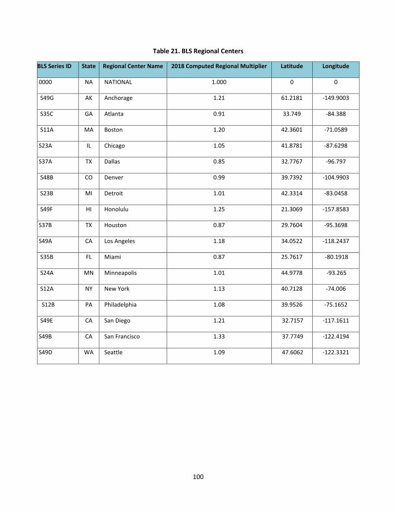
100

Table 21. BLS Regional Centers

BLS Series ID State Regional Center Name 2018 Computed Regional Multiplier Latitude Longitude

0000 NA NATIONAL 1.000 0 0

S49G AK Anchorage 1.21 61.2181 -149.9003

S35C GA Atlanta 0.91 33.749 -84.388

S11A MA Boston 1.20 42.3601 -71.0589

S23A IL Chicago 1.05 41.8781 -87.6298

S37A TX Dallas 0.85 32.7767 -96.797

S48B CO Denver 0.99 39.7392 -104.9903

S23B MI Detroit 1.01 42.3314 -83.0458

S49F HI Honolulu 1.25 21.3069 -157.8583

S37B TX Houston 0.87 29.7604 -95.3698

S49A CA Los Angeles 1.18 34.0522 -118.2437

S35B FL Miami 0.87 25.7617 -80.1918

S24A MN Minneapolis 1.01 44.9778 -93.265

S12A NY New York 1.13 40.7128 -74.006

S12B PA Philadelphia 1.08 39.9526 -75.1652

S49E CA San Diego 1.21 32.7157 -117.1611

S49B CA San Francisco 1.33 37.7749 -122.4194

S49D WA Seattle 1.09 47.6062 -122.3321

101

Table 22. National BLS Variables and Model Coefficients

BLS Variable Model

Coefficients

Model Year Values (2018)

Anchorage National

Ready-mix concrete manufacturing 0.113 NA – use national

275.5

Tractor shovel loaders (skid steer, wheel, crawler, and integral design backhoes) 0.325

NA – use national

252.3

Energy 0.096 297.492 219.941

Fuels and utilities 0.398 333.313 241.554

NA – Not Applicable

102

Post-Processing For the long-term continuous simulation of rainfall / runoff, the calculator runs its site model through SWMM using a 5-minute computational time step over each year of the period of record selected by the user, and requests that SWMM use a 15-minute reporting interval for its results. SWMM writes the rainfall intensity and the runoff results it computes at this reporting interval to a binary output file. The calculator then reads this output file and aggregates rainfall and runoff into daily totals, expressed as inches, for each day of the simulation period. It also keeps track of how many previous days occur with no measurable rainfall, for each day with measurable rainfall. Measurable rainfall and runoff is taken as any daily amount above the user-supplied threshold (whose default is 0.1 inches). For days that have runoff but no rainfall, the runoff is added to that of the previous day. After the aggregation process is complete, the long-term simulation results have been distilled down into a set of records equal in number to the number of days with measurable rainfall; where each record contains a daily rainfall, daily runoff, and number of antecedent dry days.

For extreme 24-hour storm events, SWMM makes a separate run for each event over a three-day time period to allow for LID storage to drain down. Each run has different values in its time series of rainfall intensities reflecting the different total depth associated with each extreme event return period. For these runs the only output recorded is the total runoff from the site.

The Summary Results report produced by the calculator (Figure 13) comes from a direct inspection of the long-term daily rainfall/runoff record. The Maximum Retention Volume statistic is simply the largest difference between daily rainfall and its corresponding runoff among all records.

The Rainfall / Runoff Event scatterplot (Figure 14) is generated by plotting daily each daily rainfall and its associated runoff for those days where rainfall exceeds the user-supplied threshold limit. For wet days where the runoff is below the threshold value, the runoff value is set to zero (i.e., there is no measurable runoff for those days).

The Rainfall / Runoff Frequency report (Figure 15) is generated by first sorting daily rainfall values by size, ignoring consecutive rainfall days if the user selected that option. The days per year for which each rainfall value is exceeded, is computed as (N – j) / Y, where N is the total number of rainfall values, j is the rank order of the rainfall in the sorted list, and Y is the total years simulated. Then each rainfall - exceedance frequency pair is plotted. The same set of operations is used to generate the runoff exceedance frequency curve, except now N is the total number of runoff values and j is the rank order of a runoff value in the sorted list.

The Runoff by Rainfall Percentile report (Figure 17) is generated as follows:

1. The daily measurable rainfall values are sorted by size and a set of different percentile values are identified (the 10, 20, 30, 40, 50, 60, 70, 75, 80, 85, 90, 95, and 99-th percentiles).

2. The days with rainfall that fall within each percentile interval are identified, honoring the user’s choice to either include or exclude consecutive wet days.

3. The total runoff from events in each interval, as a percentage of the total runoff from all events, is computed and plotted.

103

The Rainfall Retention Frequency report (Figure 21) is generated by taking the same set of rainfall percentiles used in the Runoff by Rainfall Percentile report, only referring to them as retention volumes. For each retention volume, the percentage of daily rainfall events providing that amount of retention is computed. This is done by examining each day with observable rainfall, ignoring back to back wet days if that option was selected. If there was no measurable runoff for the day, then the count of retained events for the retention volume being analyzed is incremented. Otherwise, if the rainfall was at least as much as the target retention and the difference between rainfall and runoff was also at least this much, then the count of retained events is also incremented. The retention provided for the given retention target is simply the number of retained events divided by the total number of daily events. This process is repeated for each of the 13 pre-selected retention volumes and the resulting pairs of retention volume – retention frequency values are plotted.

The Extreme Event Rainfall / Runoff report (Figure 23) is generated by simply plotting the rainfall and accompanying computed runoff in stacked fashion for each extreme event return period.

104

7. References

American Society of Civil Engineers (ASCE) (1992). “Design and Construction of Urban Stormwater Management Systems.” American Society of Civil Engineers, New York, NY.

Aqua Terra Consultants (2011). “Quality Assurance Project Plan – Stormwater Calculator Technical Support.” EPA Contract #EP-C-06-029, Work Assignments #4-38 and 5-38.

Center for Neighborhood Technology (2009). “National Stormwater Management Calculator.” <http://greenvalues.cnt.org/national/calculator.php>

Chen, C.W. and Shubinski, R.P. (1971). “Computer Simulation of Urban Storm Water Runoff.” Journal of the Hydraulics Division. ASCE, 97(2):289-301.

Clear Creek Solutions, Inc. (2006). “Western Washington Hydrology Model Version 3.0 User Manual.” <http://www.ecy.wa.gov/programs/wq/stormwater/wwhm_training/wwhm/wwhm_v3/index.html>

Crawford, N.H. and Linsley, R.K. (1966). “Digital Simulation in Hydrology: Stanford Watershed Model IV.” Technical Report No. 39, Civil Engineering Department, Stanford University, Palo Alto, CA.

Engman, E.T. (1986). “Roughness Coefficients for Routing Surface Runoff.” Journal of Irrigation and Drainage Engineering, ASCE, 112(1):39-53.

IPCC (Intergovernmental Panel on Climate Change) (2007). Climate Change 2007: Synthesis Report -Summary for Policymakers. Available online at: http://www.ipcc.ch/pdf/assessment-report/ar4/syr/ar4_syr.pdf

Karl, T.R., Melillo, J.M., and Peterson, T.C. (eds.) (2009). Global Climate Change Impacts in the United States. Cambridge University Press.

Meehl, G. A., C. Covey, T. Delworth, M. Latif, B. McAvaney, J. F. B. Mitchell, R. J. Stouffer, and K. E. Taylor. (2007). “The WCRP CMIP3 multi-model dataset: A new era in climate change research”, Bulletin of the American Meteorological Society, 88, 1383-1394.

Mein, R.G. and Larson, C.L. (1973). “Modeling infiltration during a steady rain.” Water Resources Research, 9(2):334-394.

Neitsch S.L., J.G. Arnold, J.R. Kiniry, and J.R. Williams (2005). “Soil and Water Assessment Tool Theoretical Documentation.” Version 2005, Agricultural Research Service and Texas Agricultural Experiment Station, January 2005.

Rawls, W.J., Brakensiel, D.L., and Miller, N. (1983). “Green-Ampt Infiltration Parameters from Soils Data”, Journal of Hydraulic Engineering, ASCE, Vol. 109, No. 1, 62-70.

Rossman, L.A. (2009). “Modeling Low Impact Development Alternatives with SWMM.” In Dynamic Modeling of Urban Water Systems, Monograph 18, W. James, ed., CHI, Guelph, ON, Canada.

RTI International and Geosyntec Consultants (2015). “Low Impact Development Stormwater Control Cost Estimation Analysis.” EPA Contract #EP-C-11-036, Task Order # 19.

105

Urban Drainage and Flood Control District (UDFCD) (2007). “Drainage Criteria Manual, Chapter 5 – Runoff”, Urban Drainage and Flood Control District, Denver, CO. (http://www.udfcd.org/downloads/down_critmanual_volI.htm).

U.S. Department of Agriculture (USDA), Natural Resources Conservation Service (NRCS) (2019). Soil Survey Geographic Database (SSURGO). https://www.nrcs.usda.gov/wps/portal/nrcs/detail/soils/survey/?cid=nrcs142p2_053627

U.S. Department of Agriculture (USDA) (1986). “Urban Hydrology for Small Watersheds, TR-55”, Natural Resources Conservation Service, USDA, Washington, DC.

U.S. Department of Agriculture (USDA) (2010). “National Engineering Handbook.” Natural Resources Conservation Service, USDA, Washington, DC.

U.S. Department of Labor, Bureau of Labor Statistics (2017). Consumer Price Index (CPI). https://www.bls.gov/cpi/

U.S. Department of Labor, Bureau of Labor Statistics (2017). Producer Price Index (PPI). https://www.bls.gov/ppi/ U.S. Environmental Protection Agency (EPA) (2016). “Storm Water Management Model Reference Manual Volume III Water Quality.” (https://nepis.epa.gov/Exe/ZyNET.exe/P100P2NY.TXT?ZyActionD=ZyDocument&Client=EPA&Index=2016+Thru+2020&Docs=&Query=&Time=&EndTime=&SearchMethod=1&TocRestrict=n&Toc=&TocEntry=&QField=&QFieldYear=&QFieldMonth=&QFieldDay=&IntQFieldOp=0&ExtQFieldOp=0&XmlQuery=&File=D%3A%5Czyfiles%5CIndex%20Data%5C16thru20%5CTxt%5C00000002%5CP100P2NY.txt&User=ANONYMOUS&Password=anonymous&SortMethod=h%7C-&MaximumDocuments=1&FuzzyDegree=0&ImageQuality=r75g8/r75g8/x150y150g16/i425&Display=hpfr&DefSeekPage=x&SearchBack=ZyActionL&Back=ZyActionS&BackDesc=Results%20page&MaximumPages=1&ZyEntry=1&SeekPage=x&ZyPURL). U.S. Environmental Protection Agency (EPA) (2016). “Summary of State Post Construction Stormwater Standards.” (https://www.epa.gov/sites/production/files/2016-08/documents/swstdsummary_7-13-16_508.pdf). U.S. Environmental Protection Agency (EPA) (2014). “Climate Change Impacts and Adapting to Change.” (http://www.epa.gov/climatechange/impacts-adaptation/).

U.S. Environmental Protection Agency (EPA) (2012). “Climate Resilience Evaluation and Awareness Tool (CREAT) Version 2.0 Methodology Guide.” (https://www.epa.gov/crwu/build-resilience-your-utility).

U.S. Environmental Protection Agency (EPA) (2010). “Storm Water Management Model User’s Manual, Version 5.0.” U.S. Environmental Protection Agency, Washington, D.C., Pub No. EPA/600/R-05/040 (Revised 2010).

U.S. Forest Service (USFS) (2014). “i-Tree Hydro User’s Manual v. 5.0.” (http://www.itreetools.org/resources/manuals.php).

106

U.S. Global Change Research Program (USGRP) (2014). “Explore Regions & Topics.” (http://www.globalchange.gov/explore).

U.S. Global Change Research Program (2018). “Fourth National Climate Assessment. Volume II: Impacts, Risks, and Adaptation in the United States.” (https://nca2018.globalchange.gov/)

Yen, B.C., (2001). “Hydraulics of Sewer Systems.” Chapter 6 in Stormwater Collection Systems Design Handbook, L.M. Mays, ed., McGraw-Hill, New York.