national transport model - working paper 2webarchive.nationalarchives.gov.uk/+/http:/ · national...

1

National Transport Model - Working Paper 2

Contents

Introduction ....................................................................................................................3

Section 1: Travel Patterns and Model Data.................................................................4

Car Ownership Model Data ..................................................................................................... 6

National Trip End Model (NTEM) Data.................................................................................. 6

Demand Model (Pass 1) Data .................................................................................................. 8

Freight Model Data .................................................................................................................. 8

Road Capacity and Costs Model (FORGE) Data..................................................................... 9

Passenger Rail Data ................................................................................................................. 9

Spend Impact Database (SID) Data ....................................................................................... 10

Section 2: Exogenous Assumptions.............................................................................11

GDP........................................................................................................................................ 11

Fuel Prices.............................................................................................................................. 11

Vehicle Emissions.................................................................................................................. 12

Values of Time....................................................................................................................... 13

Assumptions Affecting Car Ownership Rates ....................................................................... 15

Passenger Rail ........................................................................................................................ 16

Bus Fares................................................................................................................................ 16

Section 3: Policy-sensitive Inputs and Policy Representation ..................................18

Local Transport ...................................................................................................................... 18

Bus and Light Rail ................................................................................................................. 18

Revenue Support .................................................................................................................... 20

Local Authority Road User (Cordon) Charging (RUC)......................................................... 20

Parking Policies ..................................................................................................................... 22

Planning and Land Use .......................................................................................................... 23

Walking and Cycling ............................................................................................................. 24

Travel Awareness Policies ..................................................................................................... 24

Local Roads ........................................................................................................................... 24

National Roads....................................................................................................................... 25

Lane Upgrades ....................................................................................................................... 25

Junction Improvements .......................................................................................................... 26


2

Passenger Rail ........................................................................................................................ 26

Freight .................................................................................................................................... 26

Growth in tonnes lifted .......................................................................................................... 26

Average Length of Haul......................................................................................................... 27


3

Introduction Inputs and assumptions used for December 2002 forecasts in "Delivering Better Transport: Progress Report"

This is the second in a series of Working Papers describing the National Transport Model. This paper outlines the forecasting assumptions that form the basis of the model and explains how typical policies are represented. In addition, it describes the underlying data on which the model is built.

Section 1 starts with a brief description of changing travel patterns observed over recent decades. It also presents some of the 2000 data and model results describing the transport system and travel behaviour in the base year.

Section 2 summarises the exogenous assumptions included in the model and the evidence from which these have been derived.

Section 3 describes those inputs which are directly susceptible to policy action, and the representation of various other policies within the model.


4

Section 1: Travel Patterns and Model Data The National Transport Model (NTM) covers all surface modes of transport, including walk and cycle. It is based on data on the trips that people make (and on evidence of the factors that explain their choices) and distinguishes between area types and person/household types in providing forecasts for each mode.

The average distance travelled each year by residents of Great Britain has risen steadily over the past 30 years (with the exception of a small fall during the recession of the early 1990s). The distance travelled by car increased by 11% between 1989/91 and 1999/2001, whereas local bus travel (outside London) decreased by 17%. Walking fell by 20% during the 1990s.1

The NTM has been developed to support policy making by illustrating how different policies interact and impact on key outcomes - particularly traffic and trips by mode, as well as congestion and emissions. The current version has been calibrated to reproduce the 1998 travel patterns observed by the National Travel Survey and short-term forecasts have been produced for 20002. The forecasts from 1998 to 2000 do not include any policy assumptions but do include other assumptions, for example, changes in fuel price, car ownership and value of time. The travel patterns forecast for 2000 are used as a basis for comparison with future year model forecasts.

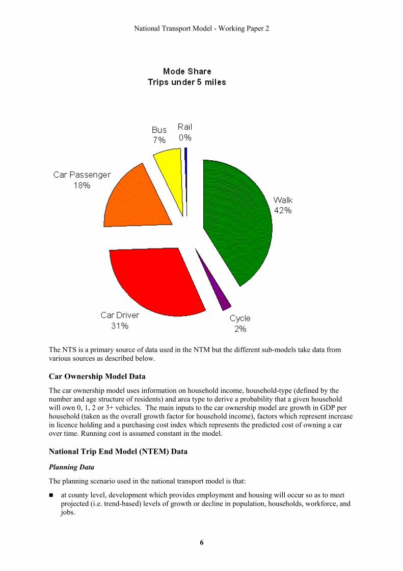
The pie chart in Figure 1 shows the modal split forecast by the NTM for the year 2000.

Figure 1

1 For further information and statistics on travel in Great Britain see the Transport Statistics Bulletin – National Travel Survey: 1999/2001 Update, National Statistics, 2002 (available at http://www.dft.gov.uk/stellent/groups/dft_control/documents/contentservertemplate/dft_index.hcst?n=7221&l=4) and Transport Statistics Great Britain 2002 Edition, The Stationery Office, October 2002 2 The model will be re-calibrated to 1999/2001 NTS data in due course.


5

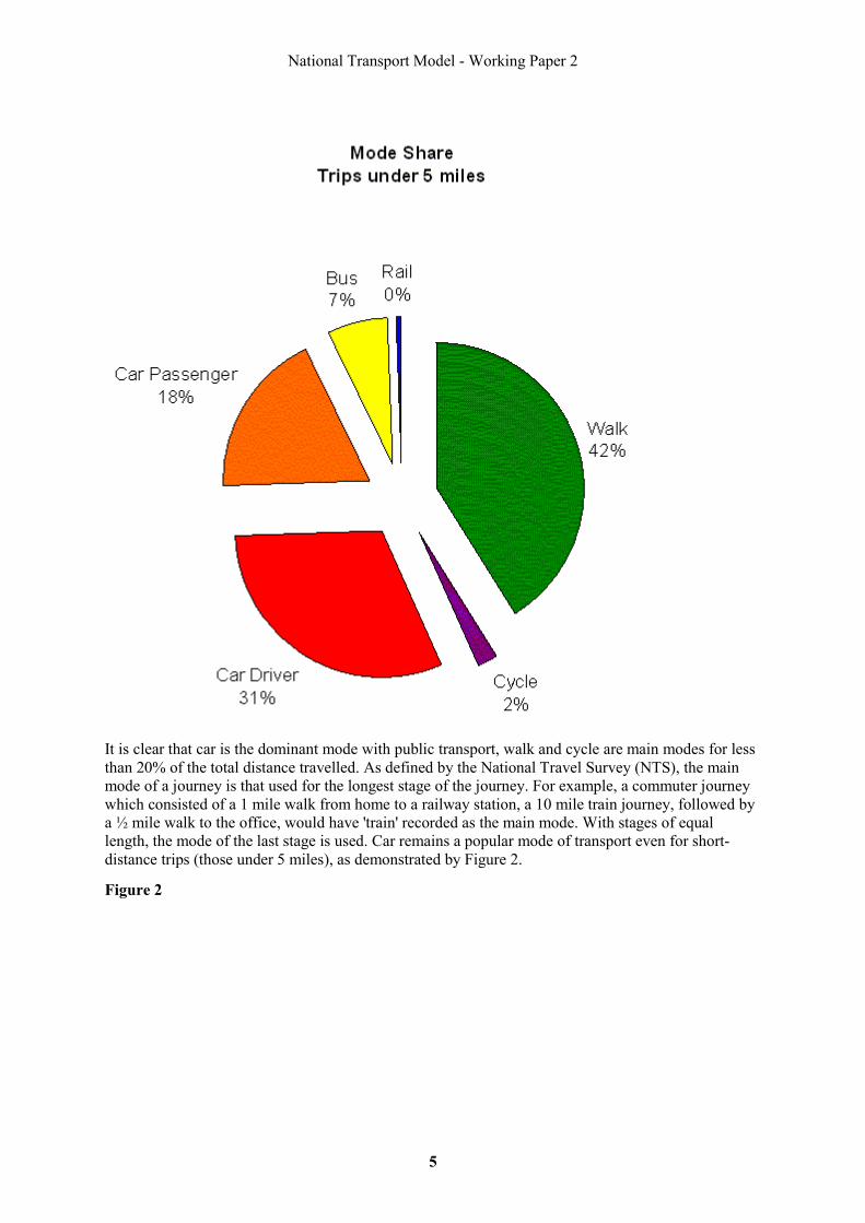
It is clear that car is the dominant mode with public transport, walk and cycle are main modes for less than 20% of the total distance travelled. As defined by the National Travel Survey (NTS), the main mode of a journey is that used for the longest stage of the journey. For example, a commuter journey which consisted of a 1 mile walk from home to a railway station, a 10 mile train journey, followed by a ½ mile walk to the office, would have 'train' recorded as the main mode. With stages of equal length, the mode of the last stage is used. Car remains a popular mode of transport even for short-distance trips (those under 5 miles), as demonstrated by Figure 2.

Figure 2


6

The NTS is a primary source of data used in the NTM but the different sub-models take data from various sources as described below.

Car Ownership Model Data

The car ownership model uses information on household income, household-type (defined by the number and age structure of residents) and area type to derive a probability that a given household will own 0, 1, 2 or 3+ vehicles. The main inputs to the car ownership model are growth in GDP per household (taken as the overall growth factor for household income), factors which represent increase in licence holding and a purchasing cost index which represents the predicted cost of owning a car over time. Running cost is assumed constant in the model.

National Trip End Model (NTEM) Data

Planning Data

The planning scenario used in the national transport model is that:

at county level, development which provides employment and housing will occur so as to meet projected (i.e. trend-based) levels of growth or decline in population, households, workforce, and jobs.


7

within each county, the distribution of households will be such as to replicate ONS short-range 1998-based population projections to 2006 and the rural-urban balance inherent in these, i.e. a continuation of present trends. The same rural-urban distribution is assumed for employment.

The four main planning variables used in the preparation of trip ends for input into the National Transport model are population, households, workforce and jobs.

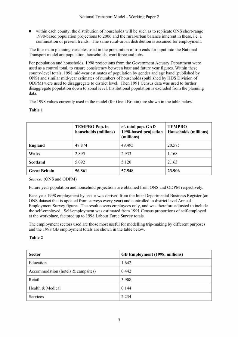
For population and households, 1998 projections from the Government Actuary Department were used as a control total, to ensure consistency between base and future year figures. Within these county-level totals, 1998 mid-year estimates of population by gender and age band (published by ONS) and similar mid-year estimates of numbers of households (published by HDS Division of ODPM) were used to disaggregate to district level. Then 1991 Census data was used to further disaggregate population down to zonal level. Institutional population is excluded from the planning data.

The 1998 values currently used in the model (for Great Britain) are shown in the table below.

Table 1

TEMPRO Pop. in households (millions)

cf. total pop. GAD 1998-based projection (millions)

TEMPRO Households (millions)

England 48.874 49.495 20.575

Wales 2.895 2.933 1.168

Scotland 5.092 5.120 2.163

Great Britain 56.861 57.548 23.906

Source: (ONS and ODPM)

Future year population and household projections are obtained from ONS and ODPM respectively.

Base year 1998 employment by sector was derived from the Inter Departmental Business Register (an ONS dataset that is updated from surveys every year) and controlled to district level Annual Employment Survey figures. The result covers employees only, and was therefore adjusted to include the self-employed. Self-employment was estimated from 1991 Census proportions of self-employed at the workplace, factored up to 1998 Labour Force Survey totals.

The employment sectors used are those most useful for modelling trip-making by different purposes and the 1998 GB employment totals are shown in the table below.

Table 2

Sector GB Employment (1998, millions)

Education 1.642

Accommodation (hotels & campsites) 0.442

Retail 3.908

Health & Medical 0.144

Services 2.234


8

Industry, Construction & Transport 9.385

Restaurants & Bars 1.140

Recreation & Sport 1.057

Agriculture & Fishing 1.036

Business 5.924

Total 26.910

Source: (Interdepartmental Business Register, Annual Employment Survey and Labour Force Survey)

From the 1998 base year position, growth rates were applied at county level, using Cambridge Econometrics projections of change in employment by sector.

To calculate the workforce, the 1998 UK total job split was obtained from the Labour Market Trend. A joint Labour Force and National Travel survey for 1998 was used to split the workforce by gender and full-time/part-time categories. Future workforce is obtained from a scenario generator model and is modelled as being determined by employment.

In addition to the planning data described above, other inputs to NTEM include population by household size and number of cars (which is an output from the car ownership model) and trip rates derived from National Travel Survey (NTS).

Demand Model (Pass 1) Data

The demand model takes the trip productions and attractions for trips by purpose and traveller type from NTEM. NTEM produces estimates of person travel by all modes (including walk and cycle) for each ward of Great Britain in the base year, as well as modal trip ends for each journey purpose.

The demand model also takes information on travel characteristics via a cost change interface, which consists of a set of linked spreadsheets allowing the spend impact database (SID) to directly adjust input parameters to the demand model.

Freight Model Data

The GB freight model contains a base year origin-destination matrix built from the following data sources:

UK Customs and Excise Trade Data

ODIT surveys (DETR, 1991 and 1996

Maritime Statistics (DTLR)

Continuing Survey of Road Goods Transport (DTLR)

Rail Freight Statistics (Railtrack)

Combining growth in tonnes lifted and average length of haul generates a forecast year origin-destination matrix.


9

Road Capacity and Costs Model (FORGE) Data

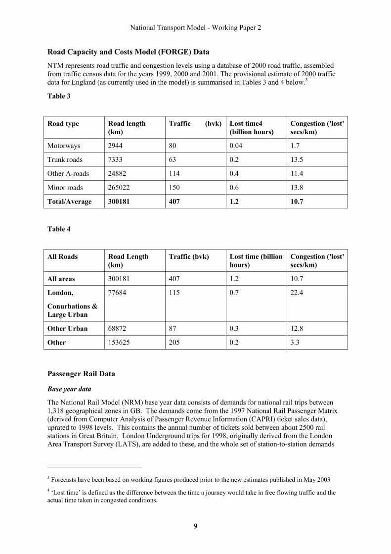
NTM represents road traffic and congestion levels using a database of 2000 road traffic, assembled from traffic census data for the years 1999, 2000 and 2001. The provisional estimate of 2000 traffic data for England (as currently used in the model) is summarised in Tables 3 and 4 below.3

Table 3

Road type Road length (km)

Traffic (bvk) Lost time4 (billion hours)

Congestion ('lost' secs/km)

Motorways 2944 80 0.04 1.7

Trunk roads 7333 63 0.2 13.5

Other A-roads 24882 114 0.4 11.4

Minor roads 265022 150 0.6 13.8

Total/Average 300181 407 1.2 10.7

Table 4

All Roads Road Length (km)

Traffic (bvk) Lost time (billion hours)

Congestion ('lost' secs/km)

All areas 300181 407 1.2 10.7

London,

Conurbations & Large Urban

77684 115 0.7 22.4

Other Urban 68872 87 0.3 12.8

Other 153625 205 0.2 3.3

Passenger Rail Data

Base year data

The National Rail Model (NRM) base year data consists of demands for national rail trips between 1,318 geographical zones in GB. The demands come from the 1997 National Rail Passenger Matrix (derived from Computer Analysis of Passenger Revenue Information (CAPRI) ticket sales data), uprated to 1998 levels. This contains the annual number of tickets sold between about 2500 rail stations in Great Britain. London Underground trips for 1998, originally derived from the London Area Transport Survey (LATS), are added to these, and the whole set of station-to-station demands

3 Forecasts have been based on working figures produced prior to the new estimates published in May 2003 4 ‘Lost time’ is defined as the difference between the time a journey would take in free flowing traffic and the actual time taken in congested conditions.


10

are then mapped to the geographical zones. Lastly, the time profile for rail trips from the National Trip-end Model (NTEM) is applied, to give a full picture of base year GB rail movements.

Base year national rail fares between zones are estimated using an econometric model of a sample of actual rail fares, on the basis of distance and ticket type. London Underground fares are simpler, and so base year Underground fares are derived from the actual prices for trips between different zone combinations.

The NRM contains a full, geographical representation of the national rail, London Underground, and Docklands Light Rail networks, and all the services operated on them, according to the 1999 summer timetable. The service data includes the capacity of each service, and the type of rolling stock from which it is formed, to inform calculations of overcrowding and emissions.

Spend Impact Database (SID) Data

The majority of the relationships contained in the spend impact database (SID) have been estimated from the available information in the Local Transport Plan (LTP) submissions and any other suitable supplementary scheme appraisals contained in the LTPs.5

5 For further details on the data contained in SID, see Research Report 3 - Spend-impact Database.


11

Section 2: Exogenous Assumptions The NTM includes various exogenous assumptions, most of which appear in both the without Plan scenario (Do Nothing) as well as the with Plan scenario.

GDP

GDP forecasts are input into various modules of the NTM, as described in National Transport Model Working Paper 1 - Structure. The GDP assumptions on which the modelling range is based are shown in Table 5 below.

Table 5

Financial Year Modelling Projection

2001-2 2.00%

2002-3 2.75%

2003-4 3.00%

2004-5 2.75%

2005-6 2.75%

2006-7 2.75%

2007-8 2.50%

2008-9 2.50%

2009-10 2.50%

Source: HMT6

The population projections between 2000 and 2010 are controlled to projections from the Government's Actuary Department7. They predict population growth of 0.336% per annum over the period 2000-05 and 0.331% per annum over the period 2005-10.

Fuel Prices

The fuel price forecasts input to the NTM are based on the DTI long run oil price projection.8 The DTI produces forecasts of oil prices from which fuel price forecasts can be derived using econometric analysis of the relationship between oil price and fuel price. The estimated elasticity of pre-tax fuel price with respect to oil price is 0.5 for unleaded petrol and 0.49 for diesel. The weighted post-tax fuel

6 Figures for 2001-2 to 2006-7 taken from Budget Report (Nov 2002), Chapter C, Table C3. Figures for 2007-8 onward taken from Economic and Fiscal Strategy Report (Budget 2002), Annex A, table A1. 7 See www.gad.gov.uk 8 The current fuel price assumptions in the NTM are based on DTI long-term oil price forecasts of $20/barrel. See http://www.dti.gov.uk/energy/


12

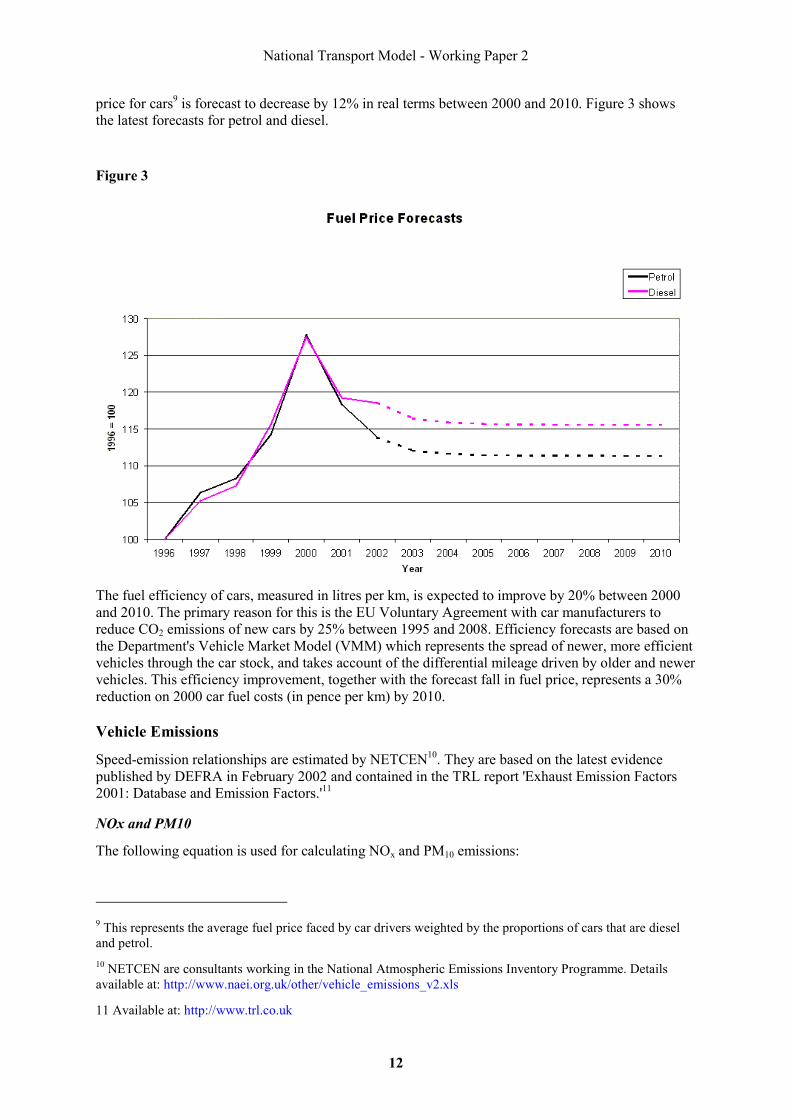
price for cars9 is forecast to decrease by 12% in real terms between 2000 and 2010. Figure 3 shows the latest forecasts for petrol and diesel.

Figure 3

The fuel efficiency of cars, measured in litres per km, is expected to improve by 20% between 2000 and 2010. The primary reason for this is the EU Voluntary Agreement with car manufacturers to reduce CO2 emissions of new cars by 25% between 1995 and 2008. Efficiency forecasts are based on the Department's Vehicle Market Model (VMM) which represents the spread of newer, more efficient vehicles through the car stock, and takes account of the differential mileage driven by older and newer vehicles. This efficiency improvement, together with the forecast fall in fuel price, represents a 30% reduction on 2000 car fuel costs (in pence per km) by 2010.

Vehicle Emissions

Speed-emission relationships are estimated by NETCEN10. They are based on the latest evidence published by DEFRA in February 2002 and contained in the TRL report 'Exhaust Emission Factors 2001: Database and Emission Factors.'11

NOx and PM10

The following equation is used for calculating NOx and PM10 emissions:

9 This represents the average fuel price faced by car drivers weighted by the proportions of cars that are diesel and petrol. 10 NETCEN are consultants working in the National Atmospheric Emissions Inventory Programme. Details available at: http://www.naei.org.uk/other/vehicle_emissions_v2.xls

11 Available at: http://www.trl.co.uk


13

NOx and PM10 Emissions (g/km) = (1-y)*(a.v3+b.v2 +c.v+d)+y*(e.v3+f. v2+g.v+h)

Where v = the speed in km/h

y = the split between diesel and petrol vehicles

All other coefficients are provided by NETCEN and differ by vehicle type.

The formula above gives NOx and PM10 emissions from vehicle engines which have been running for some time and have therefore warmed up (known as hot exhaust emissions). A similar estimate is calculated for NOx and PM10 emissions that occur when vehicles' engines initially start and are cold (cold start emissions).

CO2

Tailpipe carbon emissions are given by the equation:

Carbon emissions (g/km)

= (1-y)*p*(a.v3+b.v2+c.v+d)+y*q*(e.v3+f. v2+g.v+h) * Efficiency

Where v = the speed in km/h

y = the split between diesel and petrol vehicles

The efficiency is calculated from the consumption figures (weighted by petrol and diesel) provided by the VMM. As efficiency improves, the index decreases.

Efficiency improvements for LGVs are assumed to be the same as those for cars (20% between 2000 and 2010) but for HGVs (artic and rigid) reference case (without Plan) efficiency is only assumed to improve by 4.4% between the years 2000 to 2010. Efficiency for PSVs is assumed to remain unchanged from 2000.

The total tailpipe emissions calculated in the base year (for GB) have been calibrated to match those published by DEFRA12 and are presented in Table 6 below.

Table 6

Emission Thousand Tonnes

NOx 806.8

PM10 29.3

CO2 31515

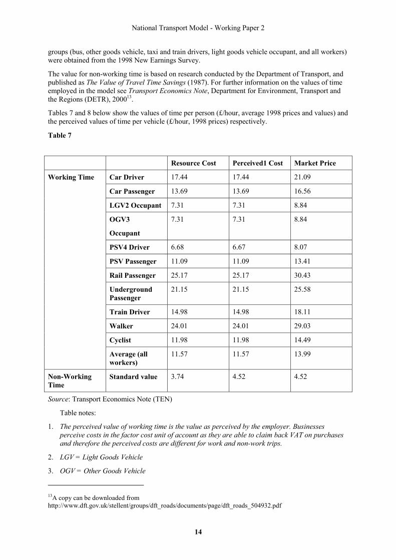
Values of Time

Different assumptions for the value of time are employed for working and non-working values of time. Working values of time apply only to journeys that are made in the course of work (this does not include commuting journeys).

Values for car drivers and passengers; rail, bus, underground and taxi passengers; walkers; cyclists; and motorcyclists were derived from the 1996/98 National Travel Survey. Values for the occupational

12 See http://www.defra.gov.uk/environment/statistics/des/airqual/alltext.htm for further details.


14

groups (bus, other goods vehicle, taxi and train drivers, light goods vehicle occupant, and all workers) were obtained from the 1998 New Earnings Survey.

The value for non-working time is based on research conducted by the Department of Transport, and published as The Value of Travel Time Savings (1987). For further information on the values of time employed in the model see Transport Economics Note, Department for Environment, Transport and the Regions (DETR), 200013.

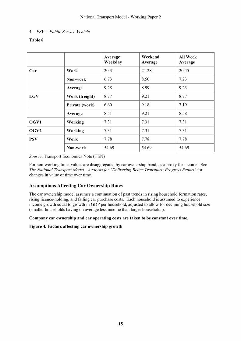
Tables 7 and 8 below show the values of time per person (£/hour, average 1998 prices and values) and the perceived values of time per vehicle (£/hour, 1998 prices) respectively.

Table 7

Resource Cost Perceived1 Cost Market Price

Car Driver 17.44 17.44 21.09

Car Passenger 13.69 13.69 16.56

LGV2 Occupant 7.31 7.31 8.84

OGV3

Occupant

7.31 7.31 8.84

PSV4 Driver 6.68 6.67 8.07

PSV Passenger 11.09 11.09 13.41

Rail Passenger 25.17 25.17 30.43

Underground Passenger

21.15 21.15 25.58

Train Driver 14.98 14.98 18.11

Walker 24.01 24.01 29.03

Cyclist 11.98 11.98 14.49

Working Time

Average (all workers)

11.57 11.57 13.99

Non-Working Time

Standard value 3.74 4.52 4.52

Source: Transport Economics Note (TEN)

Table notes:

1. The perceived value of working time is the value as perceived by the employer. Businesses perceive costs in the factor cost unit of account as they are able to claim back VAT on purchases and therefore the perceived costs are different for work and non-work trips.

2. LGV = Light Goods Vehicle

3. OGV = Other Goods Vehicle

13A copy can be downloaded from http://www.dft.gov.uk/stellent/groups/dft_roads/documents/page/dft_roads_504932.pdf


15

4. PSV = Public Service Vehicle

Table 8

Average Weekday

Weekend Average

All Week Average

Work 20.31 21.28 20.45

Non-work 6.73 8.50 7.23

Car

Average 9.28 8.99 9.23

Work (freight) 8.77 9.21 8.77

Private (work) 6.60 9.18 7.19

LGV

Average 8.51 9.21 8.58

OGV1 Working 7.31 7.31 7.31

OGV2 Working 7.31 7.31 7.31

Work 7.78 7.78 7.78 PSV

Non-work 54.69 54.69 54.69

Source: Transport Economics Note (TEN)

For non-working time, values are disaggregated by car ownership band, as a proxy for income. See The National Transport Model - Analysis for "Delivering Better Transport: Progress Report" for changes in value of time over time.

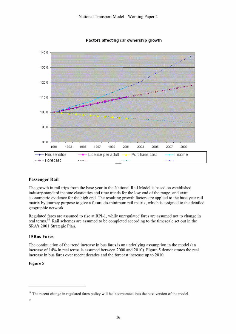
Assumptions Affecting Car Ownership Rates

The car ownership model assumes a continuation of past trends in rising household formation rates, rising licence-holding, and falling car purchase costs. Each household is assumed to experience income growth equal to growth in GDP per household, adjusted to allow for declining household size (smaller households having on average less income than larger households).

Company car ownership and car operating costs are taken to be constant over time.

Figure 4. Factors affecting car ownership growth


16

The growth in rail trips from the base year in the National Rail Model is based on established industry-standard income elasticities and time trends for the low end of the range, and extra econometric evidence for the high end. The resulting growth factors are applied to the base year rail matrix by journey purpose to give a future do-minimum rail matrix, which is assigned to the detailed geographic network.

Regulated fares are assumed to rise at RPI-1, while unregulated fares are assumed not to change in real terms.14 Rail schemes are assumed to be completed according to the timescale set out in the SRA's 2001 Strategic Plan.

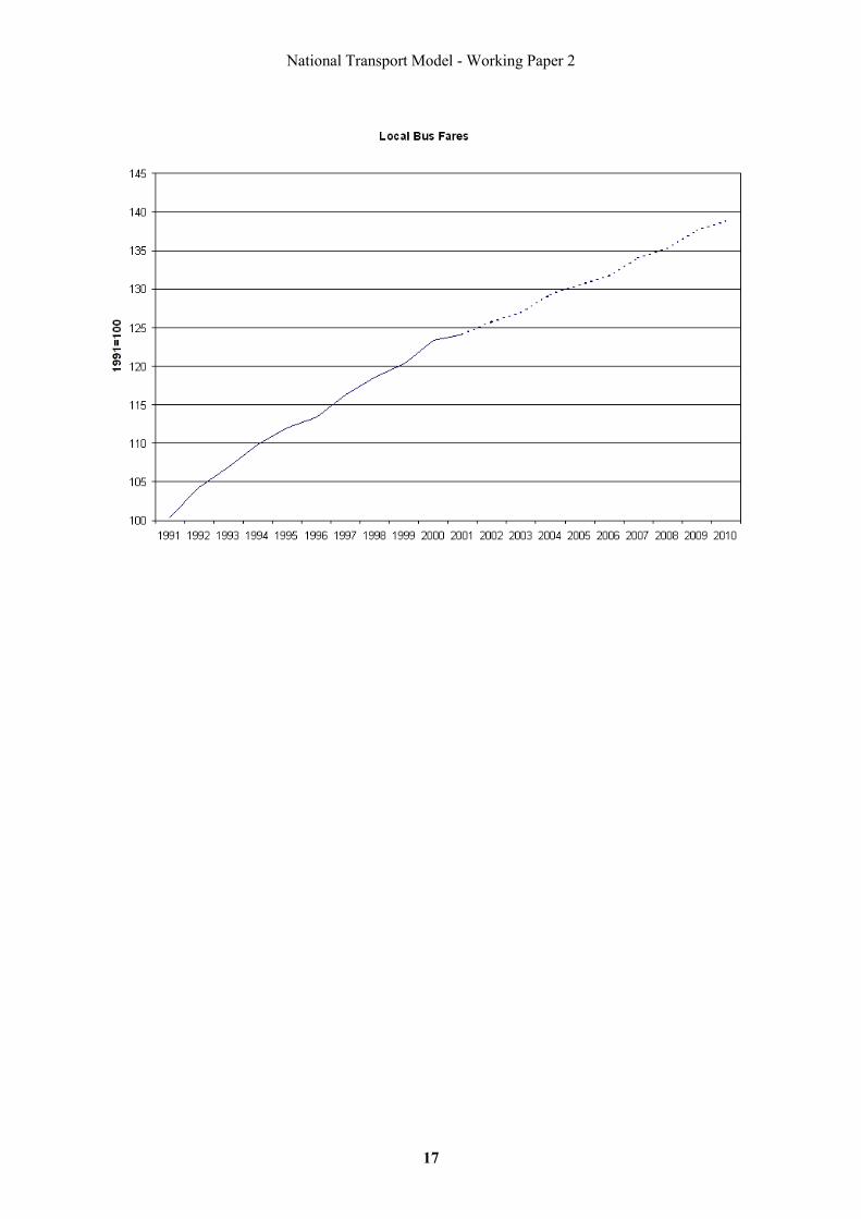
15Bus Fares

The continuation of the trend increase in bus fares is an underlying assumption in the model (an increase of 14% in real terms is assumed between 2000 and 2010). Figure 5 demonstrates the real increase in bus fares over recent decades and the forecast increase up to 2010.

Figure 5

14 The recent change in regulated fares policy will be incorporated into the next version of the model. 15

Passenger Rail


17


18

Section 3: Policy-sensitive Inputs and Policy Representation

Local Transport

A key function of the model is to provide estimates of how different levels of expenditure on local measures would affect travel by different modes. To facilitate this, a Spend-impact Database (SID) has been developed by WS Atkins to translate assumptions on local transport policies into some measure of the change in generalised cost.16 SID provides a means of defining the intensity of implementation of certain measures and calculating the impact they have on generalised cost.

In order to estimate a spend-impact relationship, a dataset is needed which provides estimates of scheme capital costs and the average change in area-wide generalised travel costs for a range of public transport schemes. The relationships contained in SID have been derived from multiple linear regression analysis of datasets containing various case study models.

The Expenditure Policy Database (EPD) was developed by WS Atkins and is a database of local transport schemes (taken from Local Transport Plans, LTPs). It contains data on the proposed level of spend on different local transport policies by English Local Authorities.17 The data is based on the December 2001 local transport settlement for local authorities (although the data on major schemes, those with a gross cost exceeding £5 million, has been updated more recently). The EPD contains details of all the local transport schemes included in the settlement. The LTPs cover the five financial year period 2001/02 to 2005/06. Schemes that are due to begin work after the financial year 2005/06 are not at present explicitly included in the EPD so a facility is used to forecast spend for future years.

The information in the database was derived from various transport models as well as a number of suitable scheme appraisals provided in the LTP submissions. The information in each database record includes the implementation cost of a public transport (PT) scheme, the average PT generalised cost change that it has been predicted to cause in the study area and the number of trips in the study area in 1998.18

Bus and Light Rail

Capital Investment

Bus and light rail investment is defined in terms of proposed total expenditure over the specified modelling period, an output from the EPD. A spend-impact relationship links the total spend on PT schemes to a change in average generalised cost of a PT trip. This relationship is derived from a database of information about the cost and impact of various PT schemes.

The spend impact relationships estimate an absolute change, in minutes, in the average generalised cost of a PT journey. The relationships currently employed in the model are shown below:

Change in Av. GC per Bus trip (mins)

= -0.3255* 3√ [(Capital expend. on Bus)

( /1998 PT trip km(£))]

* 1 (/Bus mode share)

16 WS Atkins, Estimating the Impacts of the Integrated Transport White Paper Policies, October 2002 (Research Report 3 - Spend-impact Database). 17 The EPD does not contain information on expenditure in London. Expenditure figures for London are provided by Transport for London. 18 For further information see WS Atkins, Development of Integrated Transport White Paper Impacts Analysis: Expenditure Policy Database, October 2002.


19

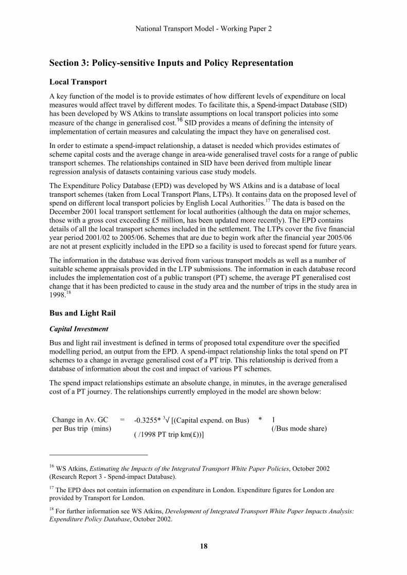
Change in Av. GC per Rail trip (mins)

= -0.0514*5√ [(Capital expend. on Rail) (/1998 PT trip km (£))]4

* 1 (/Rail mode share)

The cost change factors are split for different cost elements of the journey (access/egress time, wait time, in-vehicle time) which are weighted according to the proportion of the total base case journey costs represented by each cost element. Table 9 below shows the proportions of overall generalised cost change assumed to apply to each element of journey cost for bus travel.

Table 9

Area Type Access/ Egress Time Wait Time In-Vehicle Time

Central London 35% 10% 55%

Inner London 30% 24% 46%

Outer London 29% 22% 49%

Inner conurbation - E 32% 21% 47%

Inner conurbation - W 34% 22% 44%

Outer conurbation - E 31% 27% 42%

Outer conurbation - W 30% 27% 43%

Urban >250K - E 32% 26% 42%

Urban >250K - W 32% 29% 39%

Urban >250K - S 32% 26% 42%

Urban >100K - E 34% 26% 40%

Urban >100K - W 33% 28% 38%

Urban >100K - S 34% 27% 39%

Urban >25K 35% 28% 37%

Small & rural 36% 21% 43%

Source: WS Atkins, Estimating the Impacts of the Integrated Transport White Paper Policies, October 2002.

The spend-impact relationships outlined above only deal with changes in journey times and not changes in perceptions of PT modes. Step changes in service quality (for example, moving from conventional bus to guided bus) are generally recognised as changing travellers' perceptions of PT. A similar change in perception may result from a significant increase in network coverage (this would be an additional effect to the change in cost calculated by the spend-impact relationship).

To reflect this change in perception, bus schemes are categorised as representing a Low, Medium or High level of change (or No Change) in service quality and coverage. These categorisations are used as indicators to reflect the extent to which the bus disutilities employed in the demand model should be adjusted to represent service quality and coverage enhancement.19

19 See Research report 3 – Spend-impact Database


20

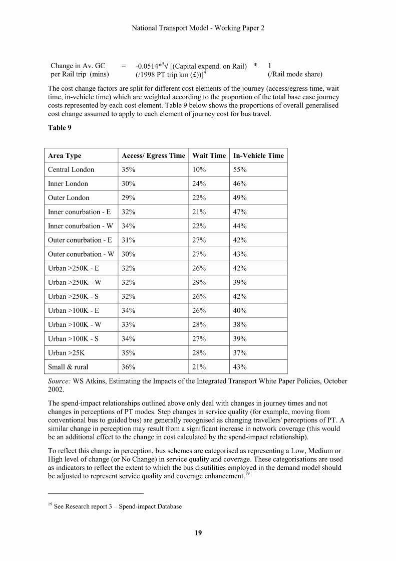
Estimates of the impact of the change in bus disutility on bus demand by area type have been made using a simple mode choice model.20 The changes in bus demand (by area type) by intensity level for service quality and coverage changes are shown in the table below.

Table 10

PT Service Quality

PT Coverage Area Type

L M H L M H

Central London 1% 3% 12%

Inner London 2% 4% 17%

Outer London 3% 6% 28%

Inner conurbation 1% 3% 13%

Outer conurbation 2% 5% 23%

Urban >250K 2% 5% 23%

Urban >100K 2% 6% 24%

Urban >25K 2% 6% 27%

0%

small & rural 3% 6% 28% 9% 18% 28%

Source: WS Atkins, Technical Note 10 - Impact Targets for Setting Modal Constant Adjustments, March 2001.

Revenue Support

The trend increase in bus fares can be counter-acted by bus revenue support, an input to SID. Estimates of the amount of expenditure required to achieve a certain percentage reduction in fares are specified within the model and the exact fare reduction is determined by interpolation. The costs of fare reductions are calculated on the basis of the amount of revenue lost due to reduced fares compared to the base case. The compensating effect of increased demand is taken into account, as is the increase in operating costs required to support any additional bus capacity necessary to carry the extra passengers.

Light rail revenue support is modelled in the same way as bus revenue support with one exception. The likely cost of rail fare reductions is calculated solely on the lost revenue costs of reduced fares (assuming that any increased demand could be accommodated within existing capacity or that additional operating costs would be borne by the operator).

Local Authority Road User (Cordon) Charging (RUC)

The average local road user charge per person for those who cross the cordon (by purpose) is a function of RUC charging policy. A relationship is derived for each journey purpose from the RUC charges input to the policy scenario. The charges are translated from a vehicle-based charge to a person-based charge on the basis of vehicle occupancy by purpose figures.

20 For further detail see WS Atkins, Technical Note 10 – Impact Targets for Setting Modal Constant Adjustments, March 2001


21

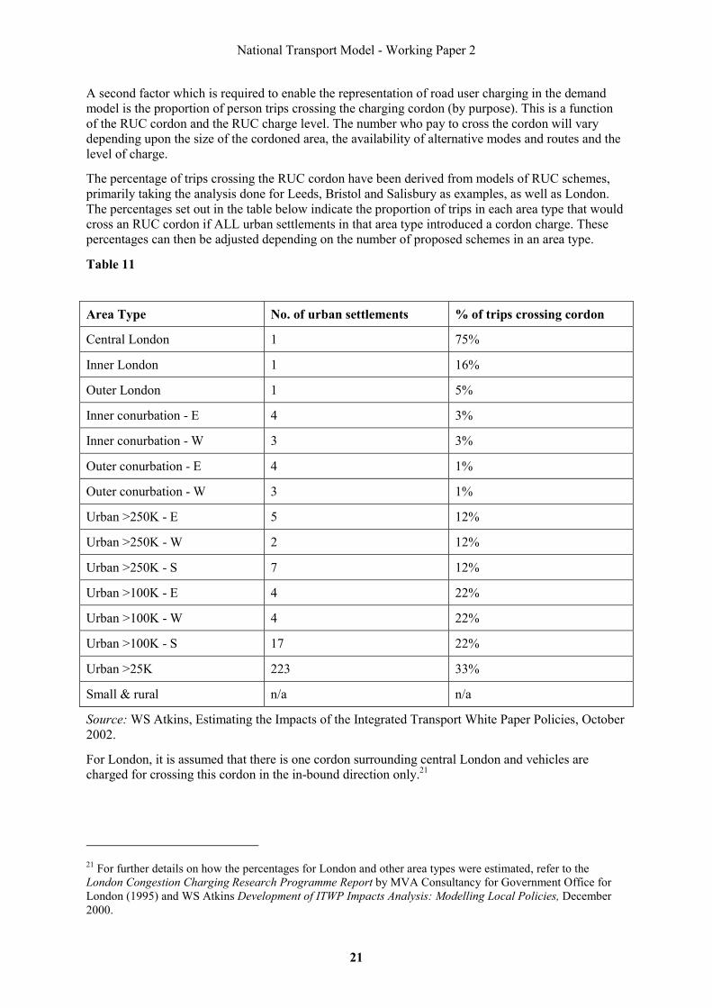
A second factor which is required to enable the representation of road user charging in the demand model is the proportion of person trips crossing the charging cordon (by purpose). This is a function of the RUC cordon and the RUC charge level. The number who pay to cross the cordon will vary depending upon the size of the cordoned area, the availability of alternative modes and routes and the level of charge.

The percentage of trips crossing the RUC cordon have been derived from models of RUC schemes, primarily taking the analysis done for Leeds, Bristol and Salisbury as examples, as well as London. The percentages set out in the table below indicate the proportion of trips in each area type that would cross an RUC cordon if ALL urban settlements in that area type introduced a cordon charge. These percentages can then be adjusted depending on the number of proposed schemes in an area type.

Table 11

Area Type No. of urban settlements % of trips crossing cordon

Central London 1 75%

Inner London 1 16%

Outer London 1 5%

Inner conurbation - E 4 3%

Inner conurbation - W 3 3%

Outer conurbation - E 4 1%

Outer conurbation - W 3 1%

Urban >250K - E 5 12%

Urban >250K - W 2 12%

Urban >250K - S 7 12%

Urban >100K - E 4 22%

Urban >100K - W 4 22%

Urban >100K - S 17 22%

Urban >25K 223 33%

Small & rural n/a n/a


For London, it is assumed that there is one cordon surrounding central London and vehicles are charged for crossing this cordon in the in-bound direction only.21

21 For further details on how the percentages for London and other area types were estimated, refer to the London Congestion Charging Research Programme Report by MVA Consultancy for Government Office for London (1995) and WS Atkins Development of ITWP Impacts Analysis: Modelling Local Policies, December 2000.


22

Parking Policies

For each destination area type and journey purpose there is an average parking search time and an average parking charge (for car trips). To calculate these averages, the overall market for parking is split into those who have to pay and those who do not.

For the paid parking market, an estimate of the paid parking supply is made from the parking search time (derived from NTS data) and the demand for parking in the base year. The level of paid parking supply can then be adjusted as a policy input for forecast years. Paid parking search time is calculated from a function of the demand for, and supply of, parking and this is the only demand responsive element in the representation of parking in the model. Parking costs and search times are averaged using a set of proportions that indicate the split between the two markets. These proportions are also a forecast year input.

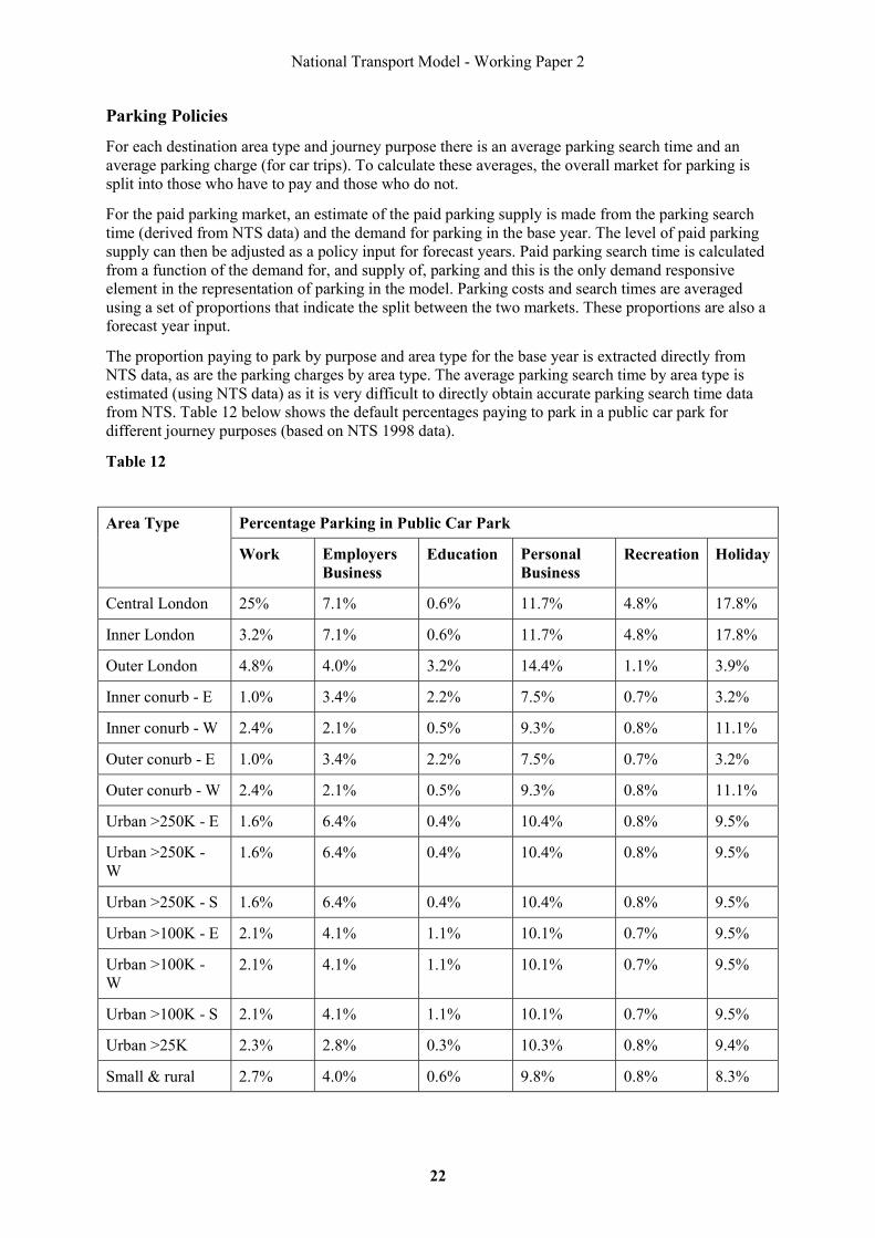
The proportion paying to park by purpose and area type for the base year is extracted directly from NTS data, as are the parking charges by area type. The average parking search time by area type is estimated (using NTS data) as it is very difficult to directly obtain accurate parking search time data from NTS. Table 12 below shows the default percentages paying to park in a public car park for different journey purposes (based on NTS 1998 data).

Table 12

Percentage Parking in Public Car Park Area Type

Work Employers Business

Education Personal Business

Recreation Holiday

Central London 25% 7.1% 0.6% 11.7% 4.8% 17.8%

Inner London 3.2% 7.1% 0.6% 11.7% 4.8% 17.8%

Outer London 4.8% 4.0% 3.2% 14.4% 1.1% 3.9%

Inner conurb - E 1.0% 3.4% 2.2% 7.5% 0.7% 3.2%

Inner conurb - W 2.4% 2.1% 0.5% 9.3% 0.8% 11.1%

Outer conurb - E 1.0% 3.4% 2.2% 7.5% 0.7% 3.2%

Outer conurb - W 2.4% 2.1% 0.5% 9.3% 0.8% 11.1%

Urban >250K - E 1.6% 6.4% 0.4% 10.4% 0.8% 9.5%

Urban >250K - W

1.6% 6.4% 0.4% 10.4% 0.8% 9.5%

Urban >250K - S 1.6% 6.4% 0.4% 10.4% 0.8% 9.5%

Urban >100K - E 2.1% 4.1% 1.1% 10.1% 0.7% 9.5%

Urban >100K - W

2.1% 4.1% 1.1% 10.1% 0.7% 9.5%

Urban >100K - S 2.1% 4.1% 1.1% 10.1% 0.7% 9.5%

Urban >25K 2.3% 2.8% 0.3% 10.3% 0.8% 9.4%

Small & rural 2.7% 4.0% 0.6% 9.8% 0.8% 8.3%


23


Planning and Land Use

The modelling of land use policies is intended to reflect the impacts of the redistribution of population and employment between area types and within built-up areas. The effects of the redistribution of population and employment between area types are accounted for in the trip-end model22 but further adjustments to car mileage rates are necessary to incorporate the impacts of land use policies within built-up areas.

National planning policy guidance is set out in PPG13 on Transport and PPG3 on Housing. PPG13 advises concentrating new residential development within or on the edge of larger settlements while PPG3 sets out procedures which should ensure that green-field sites on the edge of towns or in more rural locations are not released whilst brown-field sites remain available.

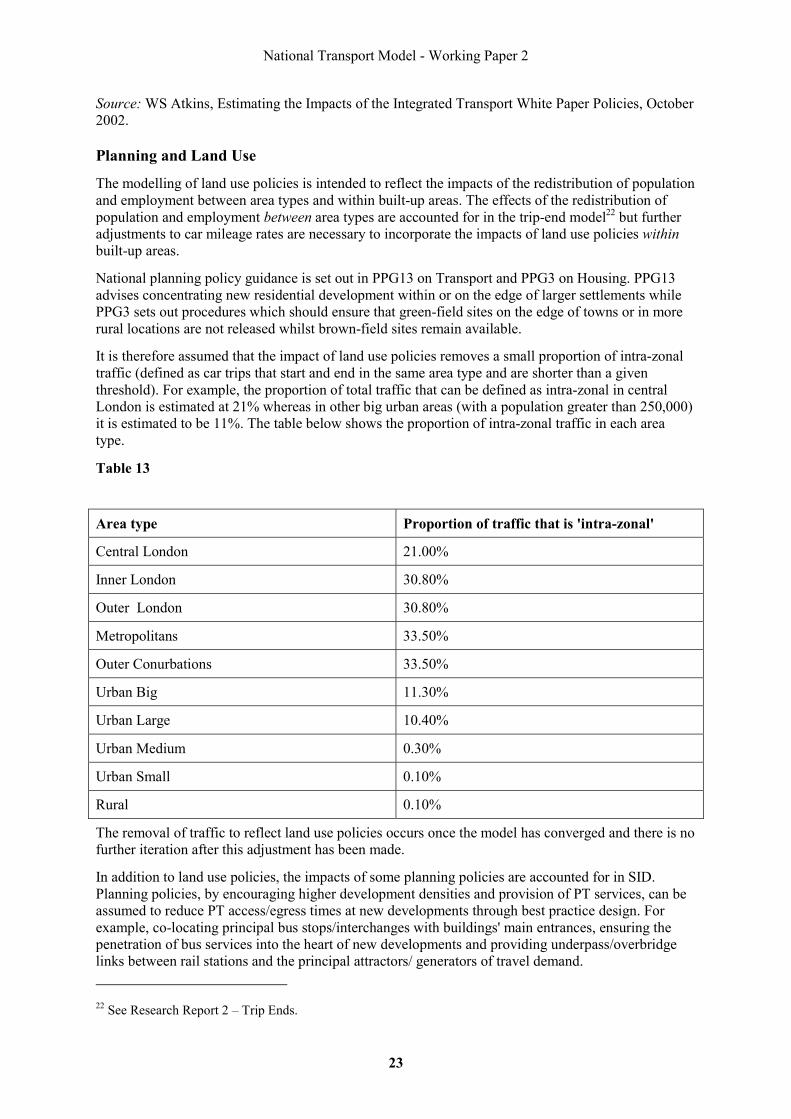
It is therefore assumed that the impact of land use policies removes a small proportion of intra-zonal traffic (defined as car trips that start and end in the same area type and are shorter than a given threshold). For example, the proportion of total traffic that can be defined as intra-zonal in central London is estimated at 21% whereas in other big urban areas (with a population greater than 250,000) it is estimated to be 11%. The table below shows the proportion of intra-zonal traffic in each area type.

Table 13

Area type Proportion of traffic that is 'intra-zonal'

Central London 21.00%

Inner London 30.80%

Outer London 30.80%

Metropolitans 33.50%

Outer Conurbations 33.50%

Urban Big 11.30%

Urban Large 10.40%

Urban Medium 0.30%

Urban Small 0.10%

Rural 0.10%

The removal of traffic to reflect land use policies occurs once the model has converged and there is no further iteration after this adjustment has been made.

In addition to land use policies, the impacts of some planning policies are accounted for in SID. Planning policies, by encouraging higher development densities and provision of PT services, can be assumed to reduce PT access/egress times at new developments through best practice design. For example, co-locating principal bus stops/interchanges with buildings' main entrances, ensuring the penetration of bus services into the heart of new developments and providing underpass/overbridge links between rail stations and the principal attractors/ generators of travel demand. 22 See Research Report 2 – Trip Ends.


24

If planning policies are implemented at a low level of intensity, it is assumed they reduce PT access/egress times by 10%, or by 40% if implementation is assumed to be high.23

Walking and Cycling

The NTM Demand Model includes walking and cycling as explicit mode choices. Given the proposed future expenditure on improving conditions for walking and cycling, some mechanism to represent the impact of this investment on the attractiveness of slow modes is required.

The approach adopted for representing slow mode schemes has been to make adjustments to the slow mode disutilities calibrated within the demand model. The scale of adjustments made in each scenario is calculated to reflect the proposed improvements. Only limited information is available on the impacts of spending on slow mode improvements. Therefore, a similar approach to that used for step changes in PT service quality has been adopted and slow mode improvements are categorised in terms of a No Change, Low, Medium or High intensity of implementation. These categorisations are used as indicators to reflect the extent to which slow mode disutilities employed in the demand model should be adjusted to represent slow mode improvements. The strength of adjustment associated with each indicator is determined using the evidence available and after discussion with DfT policy divisions.

The disutility adjustment effectively involves giving walkers and cyclists 'gifts' of time to reduce the perceived costs associated with their journeys. Rural walkers and cyclists typically require larger 'gifts' than urban walkers and cyclists. Time 'gifts' are calculated individually for different area type/distance band combinations.

Travel Awareness Policies

A similar approach to that for slow modes has been adopted for travel awareness measures. An indicator for each area type (representing the scale and intensity of application of travel awareness measures) is input and this reflects the extent to which the disutilities used within the demand model should be adjusted to represent the impact of travel awareness policies.

The actual adjustments to disutilities associated with each indicator have been calculated on the basis of estimates of the percentage reductions in traffic levels that would be caused by the different intensities of travel awareness policies. Trial runs of the model were undertaken in which the disutilities were adjusted until the model outputs replicated the estimated traffic impacts. As for walking and cycling, the extent of the percentage reductions is based on the available evidence and discussions with policy divisions. The percentage reductions that are input are not necessarily output as other components of journey cost change and therefore also determine the forecast year mode shift.

It is assumed that travel awareness policies mainly consist of workplace and school travel plans and therefore only affect journeys for work, business and education purposes. The adjustments to disutilities made in the demand model to represent travel awareness policies are therefore only applied to work, business and education related trips.

Local Roads

Local roads are considered to be those roads which do not form part of the strategic road network. Investment in local roads is defined as all roads investment that will change conditions on the local (non-strategic) road network relative to the year 2000 (but does not include road maintenance). The impact of adding additional local roads is modelled by adjusting the speed flow curves24 in the road capacity and costs model (FORGE). Assumptions about the numbers of additional local roads are

23 For further explanation see WS Atkins, Development of ITWP Impacts Analysis: Modelling Local Policies, December 2000 24 The current Speed Flow Curves used by the model are described in Research Report 8 - FORGE


25

derived from estimates of the numbers of new developments and estate roads stemming from land use changes and from specific schemes contained in Local Transport Plans.

Additional road capacity contained in new developments is only assumed to occur in Outer London, Outer Conurbations and other Urban Areas, and only applies to minor roads. Minor road growth is taken as 0.5% per annum in Urban area types and 0.15% per annum in Outer London and Conurbations,

More scheme specific investment in local roads is calculated from Local Authorities' Local Transport Plans (LTPs) by the EPD. The relationships between spend and changes in local road capacity were estimated using information available from the LTP submissions. The LTPs provided the Local Authorities' statements on the funds required for different types of road scheme and an estimate of the delivery of different types of scheme in terms of kilometres of new road or number of schemes.

Relationships of the following form were estimated:

Change in road kms = spend on road schemes / (cost/km)

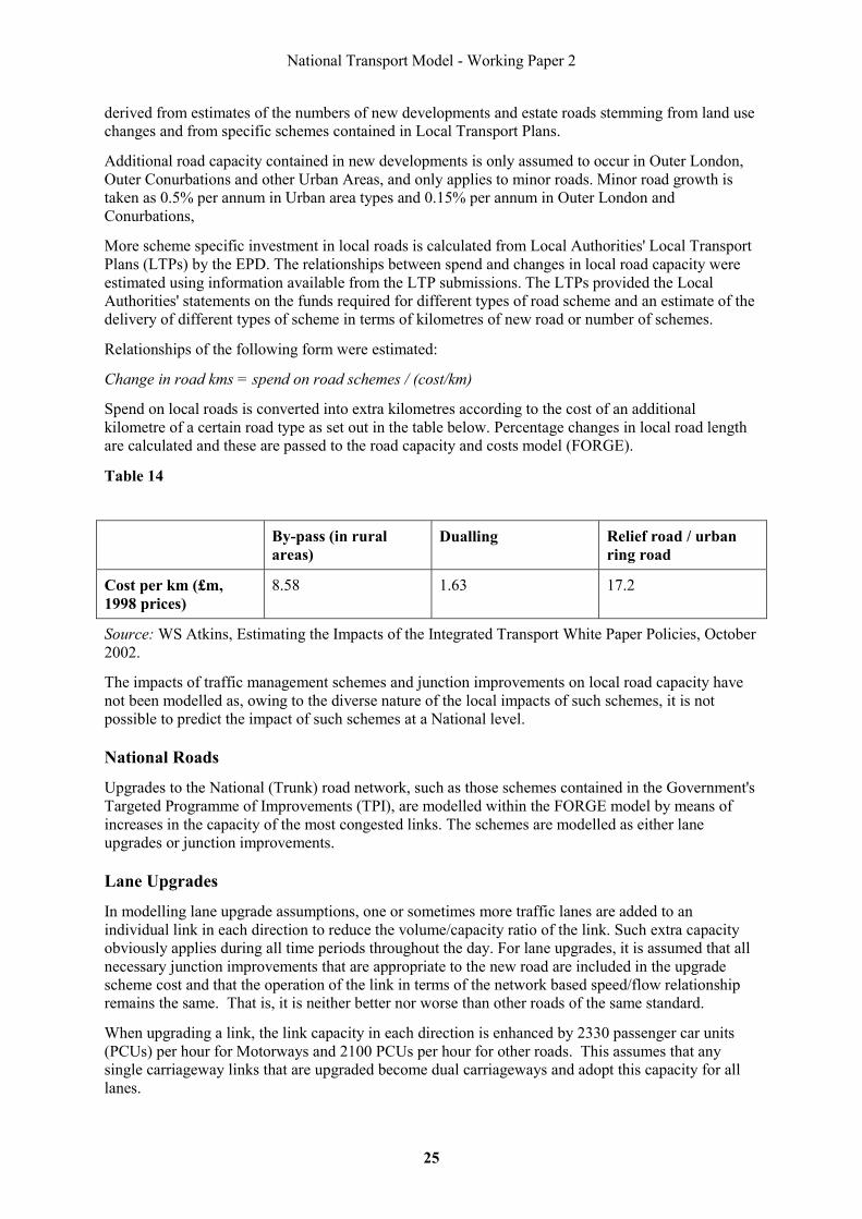
Spend on local roads is converted into extra kilometres according to the cost of an additional kilometre of a certain road type as set out in the table below. Percentage changes in local road length are calculated and these are passed to the road capacity and costs model (FORGE).

Table 14

By-pass (in rural areas)

Dualling Relief road / urban ring road

Cost per km (£m, 1998 prices)

8.58 1.63 17.2


The impacts of traffic management schemes and junction improvements on local road capacity have not been modelled as, owing to the diverse nature of the local impacts of such schemes, it is not possible to predict the impact of such schemes at a National level.

National Roads

Upgrades to the National (Trunk) road network, such as those schemes contained in the Government's Targeted Programme of Improvements (TPI), are modelled within the FORGE model by means of increases in the capacity of the most congested links. The schemes are modelled as either lane upgrades or junction improvements.

Lane Upgrades

In modelling lane upgrade assumptions, one or sometimes more traffic lanes are added to an individual link in each direction to reduce the volume/capacity ratio of the link. Such extra capacity obviously applies during all time periods throughout the day. For lane upgrades, it is assumed that all necessary junction improvements that are appropriate to the new road are included in the upgrade scheme cost and that the operation of the link in terms of the network based speed/flow relationship remains the same. That is, it is neither better nor worse than other roads of the same standard.

When upgrading a link, the link capacity in each direction is enhanced by 2330 passenger car units (PCUs) per hour for Motorways and 2100 PCUs per hour for other roads. This assumes that any single carriageway links that are upgraded become dual carriageways and adopt this capacity for all lanes.


26

Junction Improvements

The modelling of a junction improvement differs from a lane upgrade in that the improvement is assumed to remove or reduce junction delays that occur during congested periods only. Although this is achieved by reducing the v/c ratio of the link during such periods, it is equivalent to putting a step into the speed/flow relationship.

The size of the step varies by road standard but, for all links, it was calibrated to represent a 2 minute time saving on an average length of link. This ranged from 3-5Km for all purpose links and was 10Km for motorways. This time saving was based on congested conditions, when the link is at a v/c of 1.0, and results in a speed improvement equivalent to a v/c reduction of 0.1 for Motorway links and 0.15 for single and dual carriageway all purpose links.

The time saving reduces when the link is below capacity and is assumed to reach zero at the cut-off value of v/c = 0.7 in the forecast year. For periods when the v/c ratio of the link is below the cut-off value, no time savings are achieved.

Three types of junction improvements are modelled and these are targeted to represent motorway junctions, other major junction improvements and smaller scale network improvements.

The major junction improvements were assumed to involve schemes such as the construction of grade separated junctions. These are applied only to dual carriageway Trunk road links that are greater than 2.5km in length.

Smaller scale junction improvements are then applied to the remaining most congested single or dual carriageway links.

Passenger Rail

The NRM contains a detailed fares matrix, showing the rail fare between each origin and destination zone pair. Due to the complexity of the fares system, these have been estimated using an econometric model of a sample of actual fares. The fares are aggregated up to the Pass1 structure, where they enter the calculation of rail generalised costs, and Pass1's calculation of mode split. Hence by altering this matrix of fares it is possible to represent the impacts of fares policy on rail demand.

The NRM also represents the set of rail services available between an origin and a destination zone in terms of the number of trains per hour, their capacity, and journey time. Rail schemes, such as the investment in rail infrastructure to increase line speeds, making services more frequent, or an increasing train length can therefore be represented, either individually or as a package, by altering the number of trains per hour, their capacity, or speed, for the areas affected.

Freight

The Department uses MDS Transmodal's Great Britain Freight Model (GBFM), which is a commodity-based model of freight traffic. The model derives a matrix of the tonnes lifted of different commodities between each origin and destination in the forecast year, working from a geographical representation of the road and rail network in Britain. These movements are then split between road and rail on the basis of the relative costs of moving freight by these two modes. Those flows that have been allocated to road are then divided between 18 HGV types, based on the least-cost routes for each type. Road freight traffic is assigned to a highly detailed road network, and growth by region, area type and road type is calculated.

Growth in tonnes lifted

GDP growth works to increase the tonnes lifted of each commodity, magnifying the base year O-D matrix. The hypothesis being that as output in the economy increases, so should the volume of freight tonnes lifted.


27

OLS regression was employed to estimate the relationship between GDP and tonnes lifted of each commodity; for most commodities sector GDP or lags of GDP were also included as regressors. The estimated parameters are then used to forecast commodity tonnes lifted, given future year GDP.

An average per annum tonnes lifted growth rate to the forecast year for each commodity is calculated, given GDP growth. In addition, average per annum growth between 1997 and 2000 for each commodity is calculated from historical data. The final commodity growths applied by the model to the base year O-D matrix are an average of the per annum regression and historical growths.

Average Length of Haul

Forecast year average length of haul is derived from its historical series. Average per annum LOH growth for the year's 1989-2000 and 1994-2000 are worked out, and the average of the two figures taken. This figure is then used to uprate actual 2000 LOH to the forecast year.

national transport model - working paper 2webarchive.nationalarchives.gov.uk/+/http:/ · national...

Documents