BACHELOR THESIS

Ludmila Tydlitatova

Native Language Identification of L2Speakers of Czech

Institute of Formal and Applied Linguistics

Supervisor of the bachelor thesis: RNDr. Jirı Hana, Ph.D.

Study programme: Computer Science

Study branch: General Computer Science

Prague 2016

I declare that I carried out this bachelor thesis independently, and only with the

cited sources, literature and other professional sources.

I understand that my work relates to the rights and obligations under the Act

No. 121/2000 Sb., the Copyright Act, as amended, in particular the fact that the

Charles University has the right to conclude a license agreement on the use of

this work as a school work pursuant to Section 60 subsection 1 of the Copyright

Act.

In ............ date ............... signature of the author

i

ii

Title: Native Language Identification of L2 Speakers of Czech

Author: Ludmila Tydlitatova

Institute: Institute of Formal and Applied Linguistics

Supervisor: RNDr. Jirı Hana, Ph.D., Institute of Formal and Applied Linguistics

Abstract: Native Language Identification is the task of identifying an author’s

native language based on their productions in a second language. The absolute

majority of previous work has focused on English as the second language. In this

thesis, we work with 3,715 essays written in Czech by non-native speakers. We

use machine learning methods to determine whether an author’s native language

belongs to the Slavic language group. By training models with different feature

and parameter settings, we were able to reach an accuracy of 78%.

Keywords: computational linguistics, machine learning, NLP, Natural Language

Processing, NLI, Native Language Identification

iii

iv

First, I would like to thank my supervisor, Jirı Hana, whose time, comments and

patience I am greatly grateful for. Next, I would like to thank Simon Trlifaj.

He created the figures in Chapter 2, proofread most of the text and provided me

with support through all stages of writing this thesis. Last but not least, I thank

my father, Borivoj Tydlitat, the best teacher one could wish for. He introduced

me to the field of computational linguistics, guided me through my studies and

provided valuable help and feedback.

v

vi

Contents

1 Introduction 3

1.1 Structure . . . . . . . . . . . . . . . . . . . . . . . . . . . . . . . 4

2 Machine Learning Background 5

2.1 Support Vector Machine Classification . . . . . . . . . . . . . . . 5

2.1.1 Large/Hard Margin Classification: Linearly Separable Data 5

2.1.2 Soft Margin Classification: Non-separable Data . . . . . . 9

2.1.3 Non-linear Classification: Kernels . . . . . . . . . . . . . . 10

2.2 Feature Selection . . . . . . . . . . . . . . . . . . . . . . . . . . . 11

2.2.1 Information gain . . . . . . . . . . . . . . . . . . . . . . . 12

2.3 Feature Types . . . . . . . . . . . . . . . . . . . . . . . . . . . . . 14

2.3.1 n-grams . . . . . . . . . . . . . . . . . . . . . . . . . . . . 15

2.3.2 Function words . . . . . . . . . . . . . . . . . . . . . . . . 15

2.3.3 Context-free Grammar Production Rules . . . . . . . . . . 16

2.3.4 Errors . . . . . . . . . . . . . . . . . . . . . . . . . . . . . 17

3 Native Language Identification Background 19

3.1 English NLI . . . . . . . . . . . . . . . . . . . . . . . . . . . . . . 19

3.1.1 Feature Types . . . . . . . . . . . . . . . . . . . . . . . . . 20

3.1.2 Cross-corpus evaluation . . . . . . . . . . . . . . . . . . . 23

3.1.3 Native Language Identification Shared Task 2013 . . . . . 24

3.2 non-English NLI . . . . . . . . . . . . . . . . . . . . . . . . . . . 26

3.2.1 Czech . . . . . . . . . . . . . . . . . . . . . . . . . . . . . 27

3.2.2 Chinese . . . . . . . . . . . . . . . . . . . . . . . . . . . . 28

3.2.3 Arabic . . . . . . . . . . . . . . . . . . . . . . . . . . . . . 29

3.2.4 Finnish . . . . . . . . . . . . . . . . . . . . . . . . . . . . 29

3.2.5 Norwegian . . . . . . . . . . . . . . . . . . . . . . . . . . . 30

4 Our work 31

4.1 Data . . . . . . . . . . . . . . . . . . . . . . . . . . . . . . . . . . 31

4.1.1 Czech Language . . . . . . . . . . . . . . . . . . . . . . . . 31

1

4.1.2 Corpus . . . . . . . . . . . . . . . . . . . . . . . . . . . . . 31

4.1.3 Our data . . . . . . . . . . . . . . . . . . . . . . . . . . . . 33

4.2 Tools . . . . . . . . . . . . . . . . . . . . . . . . . . . . . . . . . . 34

4.3 Features . . . . . . . . . . . . . . . . . . . . . . . . . . . . . . . . 35

4.3.1 n-grams . . . . . . . . . . . . . . . . . . . . . . . . . . . . 35

4.3.2 Function words . . . . . . . . . . . . . . . . . . . . . . . . 35

4.3.3 Average length of word and sentence . . . . . . . . . . . . 36

4.3.4 Errors . . . . . . . . . . . . . . . . . . . . . . . . . . . . . 36

4.4 Experiments on development data . . . . . . . . . . . . . . . . . . 36

4.4.1 Run 1 . . . . . . . . . . . . . . . . . . . . . . . . . . . . . 37

4.4.2 Run 2 . . . . . . . . . . . . . . . . . . . . . . . . . . . . . 39

4.4.3 Run 3 . . . . . . . . . . . . . . . . . . . . . . . . . . . . . 40

4.5 Results . . . . . . . . . . . . . . . . . . . . . . . . . . . . . . . . . 41

Conclusion 45

Bibliography 47

Appendices 53

A Czesl-SGT – Metadata 53

B Prague Positional Tagset 55

C CzeSL-SGT – Errors 57

D Experiments – Run 1 59

E Experiments – Run 2 61

F Experiments – Run 3 63

G Features by Information Gain – Selected plots 65

H Top features by Information Gain – Examples 67

Attachments 71

2

1. Introduction

In today’s global context, learning of second languages is common. For example,

in Europe, beginning to learn a second language in elementary school and a third

one around age 12 has become almost routine.1 Considering the amount of ma-

terial produced in non-native languages every day in combination with the power

of Natural Language Processing (NLP), a broad field of research opportunities

has opened.

Imagine you are given a text in your native language from an unknown author.

It would probably not be a hard task to infer whether the author is a native

speaker of the text’s language or not. A much more demanding question is, what

can we say about the native language of the author? What family does his native

language belong to? Given that we suspect a particular set of languages (maybe

we know that the author comes from Asia), with what probability would we

assign them to his native language? These and other questions are addressed by

research in the field of Native Language Identification (NLI).

Due to recent research, it seems that machine learning algorithms outperform

humans in the task of NLI:

– Modifying the task of NLI to identifying the native language group, Ahar-

odnik et al. [2013] conducted an experiment with native speakers of Czech

and Czech essays. The participants, all of which had some previous train-

ing in linguistics, read as many randomly assigned essays as they wanted

and predicted the author’s native language group (Indo-European or Non-

Indo-European) based on their intuitions. An average accuracy of 55% was

achieved, only slightly higher than the 50% baseline.

– Malmasi et al. [2015b] designed a similar experiment: each of the ten partic-

ipants classified 30 English essays into 5 language classes (Arabic, Chinese,

German, Hindi, Spanish). On average, the raters correctly identified about

37% of essays (approximately 11 essays).

1http://www.pewresearch.org/fact-tank/2015/07/13/learning-a-foreign-

language-a-must-in-europe-not-so-in-america/ft_15-07-13_foreignlanguage_

histogram/

3

An absolute majority of work in the area of NLI has been carried out on English

texts. Even though not all of the results are comparable (due to the reasons

discussed below), we can say that overall, accuracy in automatic classification

repeatedly reaches 80% and more. Previous work has concentrated on various

aspects of language: phonology-motivated approaches examine the character level

of texts, other researchers focus on words and their characteristics such as their

part of speech. A considerable amount of investigation has been carried out on

syntactic aspects of sentences.

Solving the task of Native Language Identification has a number of appli-

cations, mainly in the fields of education (teaching by materials which respect

the learner’s native language, native language-specific feedback to learners) and

forensics (extracting information from anonymous texts).

We address a modified problem of Native Language Identification (NLI), test-

ing whether an author’s native language belongs to the Slavic language group or

not.

1.1 Structure

This study is structured as follows:

In Chapter 2 we introduce some concepts from machine learning, mainly Sup-

port Vector Machines (SVMs) and classification with them. Then we provide an

overview of types of features that we use in our experiments.

In Chapter 3 we present related work, distinguishing between work carried

out on English and non-English data.

In Chapter 4 we describe the data that we use, the features that we chose and

their representation. Next we give a summary of our experiments, together with

their results.

4

2. Machine Learning Background

2.1 Support Vector Machine Classification

In a general n-ary text classification task, we are given a document represented

by a vector x ∈ X and a set of n classes Y = {y1, y2, . . . , yn}. Then using a

learning method, we want to learn a decision function f that maps documents to

classes:

f : X→ Y.

This decision function will (in an ideal case) allow us to map new unseen exam-

ples. This process is commonly referred to as supervised learning, in contrast to

unsupervised learning, where no explicit labels are assigned to data and the learn-

ing method only works with observed patterns and extracted statistical structure.

We will further on generally assume a binary classification task. Documents

are represented as feature vectors xi ⊆ Rn and we work with a set of training

data

{xi, yi}di=1

from which the decision function f : Rn → Y is learned. Here d is the number of

training examples and yi ∈ {−1,+1} denote the class labels.

In the following three subsections, we will first concentrate on the simplest

task – classifying linearly separable data with Support Vector Machines (SVMs),

next we explain how the method is applied to general unseparable data containing

outliers (observations with extreme values) or noisy data (corrupted observations)

and in the third section we focus on how SVMs deal with data that does not allow

linear separation at all.

2.1.1 Large/Hard Margin Classification: Linearly Sepa-

rable Data

Consider the datasets in Figures 2.1 and 2.2, both of which consist of two classes.

Clearly both of the datasets are somehow separable. In 2.1, we can separate the

two classes perfectly by drawing a line between them. In 2.2, we can separate the

5

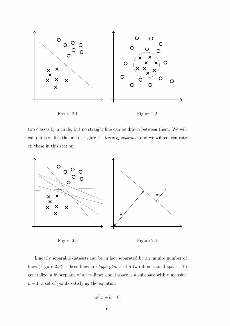
Figure 2.1 Figure 2.2

two classes by a circle, but no straight line can be drawn between them. We will

call datasets like the one in Figure 2.1 linearly separable and we will concentrate

on these in this section.

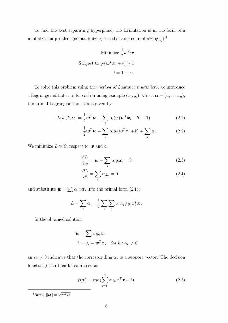
Figure 2.3

b

w

Figure 2.4

Linearly separable datasets can be in fact separated by an infinite number of

lines (Figure 2.3). These lines are hyperplanes of a two dimensional space. To

generalize, a hyperplane of an n-dimensional space is a subspace with dimension

n− 1, a set of points satisfying the equation

wTx+ b = 0,

6

where w, the parameter vector or weight vector, is normal (orthogonal to any

vector lying on the hyperplane), x is the vector representation of the document

and b ∈ R moves the hyperplane in the direction of w (See Figure 2.4). The form

of the decision function for document x can now be defined as

f(x) = sgn(wTx+ b),

a value of −1 indicating one class and +1 indicating the other class.

Given a data set and a particular hyperplane, the functional margin φi of an

example xi is defined as yi(wTxi + b) (. . . ) and the geometric margin γi

γi =φi‖w‖

=|f(xi)|‖w‖

gives us the Euclidean distance between xi and the hyperplane.

A Support Vector Machine (SVM) (Vapnik [1979],Vapnik and Kotz [1982]) is

a hyperplane based classifier that in addition to finding a separating hyperplane

defines it to be as far away from the nearest data instances (the support vectors)

as possible. That is it maximizes the margin of the classifier γ = 2‖w‖ , which is

the width of the band drawn between the data instances closest to the hyperplane

(Figure 2.5).

γ

b

w

Figure 2.5

7

To find the best separating hyperplane, the formulation is in the form of a

minimization problem (as maximizing γ is the same as minimizing 1γ):1

Minimize1

2wTw

Subject to yi(wTxi + b) ≥ 1

i = 1 . . . n.

To solve this problem using the method of Lagrange multipliers, we introduce

a Lagrange multiplier αi for each training example (xi, yi). Given α = (αi . . . αn),

the primal Lagrangian function is given by

L(w, b,α) =1

2wTw −

∑i

αi(yi(wTxi + b)− 1) (2.1)

=1

2wTw −

∑i

αiyi(wTxi + b) +

∑i

αi (2.2)

We minimize L with respect to w and b:

∂L

∂w= w −

∑i

αiyixi = 0 (2.3)

∂L

∂b=∑i

αiyi = 0 (2.4)

and substitute w =∑

i αiyixi into the primal form (2.1):

L =∑i

αi −1

2

∑i

∑j

αiαjyiyjxTi xj

In the obtained solution

w =∑

αiyixi

b = yk −wTxk for k : αk 6= 0

an αi 6= 0 indicates that the corresponding xi is a support vector. The decision

function f can then be expressed as

f(x) = sgn(n∑i=1

αiyixTi x+ b). (2.5)

1Recall ‖w‖ =√wTw

8

2.1.2 Soft Margin Classification: Non-separable Data

In the context of real-world tasks, data are seldom perfectly (and linearly) sepa-

rable. A soft margin SVM allows outliers to exist within the margin, but pays a

cost for each of them. Slack variables ξi are introduced for each data instance to

prevent the outliers from affecting the decision function:

ξi =

0, if xi is correctly classified,

≤ 1‖w‖ , if xi violates the margin rule,

> 1‖w‖ if xi is misclassified.

(2.6)

In Figure 2.6, document x1 is misclassified and document x2 violates the

margin rule:

γ

x1 x2

Figure 2.6: Slack variables

The formulation of the SVM optimization problem with slack variables is now:

Minimize1

2wTw + C ·

n∑i=1

ξi

Subject to yi(wTxi + b) ≥ 1− ξi

i = 1 . . . n,

where the cost parameter C ≥ 0 provides a way to control overfitting of data.

This occurs when the learning process provides a very accurate fit to the training

9

data, but cannot generalize on unseen testing data: a small value of C results in a

large margin while a large C results in a narrow margin, classifying more training

examples correctly (the soft-margin SVM then behaves as the hard-margin SVM).

Figure 2.7: Small C Figure 2.8: Large C

The solution of the minimization problem with slack variables is

w =∑

αiyixi

b = yk(1− ξk)−wTxk for k = arg maxk

αk

and the decision function follows 2.5.

2.1.3 Non-linear Classification: Kernels

Consider now the data set in Figure 2.9, which contains data instances of one

dimension:

0 x

Figure 2.9

Clearly we are unable to separate the data by a linear classifier.2 But by

2Recall also Figure 2.2

10

projecting the data into a space of higher dimension, we can make it linearly

separable (Figure 2.10).

x

x2

0

Figure 2.10: φ(x) = (x, x2)

As finding the mapping φ can turn out to be expensive (due to it’s high

dimension), SVMs provide an efficient method, commonly reffered to as the kernel

trick : we do not need to explicitly define the mapping φ, but instead we define a

kernel function

K : Rn × Rn → R (2.7)

K(xi,xj) = φ(xTi )φ(xj) (2.8)

and replace the dot product xixj :

L(α) =∑

αi −1

2

∑αiαjyiyjK(xi,xj) (2.9)

f(x) = sgn(n∑i=1

αiyiK(xi,x) + b). (2.10)

Common kernel functions include:

K(xi,xj) =

xTi xj (linear),

(s · xTi xj + r)d (polynomial),

e−γ·‖xi−xj‖2 (radial basis function (RBF)),

(2.11)

where r, s, γ > 0 are user-defined parameters.

2.2 Feature Selection

In machine learning experiments, commonly a subset of all available features is

chosen, dealing with two potential issues: First, irrelevant features induce greater

11

computational cost and, second, irrelevant features may lead to overfitting. The

process of selecting a feature subset is reffered to as feature selection. A multitude

of feature selection techniques exist. When applying filter methods of selection,

the features are first ranked based on a relevance to class measure, then a subset

is selected and this subset is given to the classifier. Popular rankings include

Pearson’s correlation coefficient, F-score or mutual information.

Wrapper methods of selection employ a classifier: first a subset of features

is chosen, then the subset is evaluated by a classifier, a change to the subset is

made and the new subset is evaluated. This approach is generally very expensive

in computation, so heuristic search methods are applied to find the optimal sets

of features.

In our experiments, we choose to filter features using the ranking of mutual

information, sometimes called information gain.

2.2.1 Information gain

Entropy of a random variable

Let p(x) be the probability function of a random variable x over the event space

X : p(x) = P (X == x). The entropy H(p) = H(X) ≥ 0 is the average uncer-

tainty of a single variable:

H(X) =∑x∈X

p(x) · log2

1

p(x)

= −∑x∈X

p(x) · log2 p(x).

Entropy measures the amount of information in a random variable, sometimes

described as the average number of 0/1 questions needed to describe an outcome

of p(x), 3 or the average number of bits you necessarily need to encode a value

of the given random variable. To describe the behavior of the entropy function,

consider the following example from Manning and Schutze [1999]:

Simplified Polynesian appears to be just a random sequence of letters, with

the following letter frequencies: Then the per-letter entropy is:

3https://en.wikipedia.org/wiki/Twenty_Questions

12

p t k a i u

18

14

18

14

18

18

H(Polynesian) = −∑

i∈{p,t,k,a,i,u}

p(i) · log2 p(i)

= −(4 · 1

8· log2

1

8+ 2 · 1

4· log2

1

4)

= 21

2bits.

Following the previous interpretation of entropy, we can now design a code that

takes on average 212

bits to encode a letter:

p t k a i u

100 00 101 01 110 111

The definition of entropy extends to joint distributions as the amount of in-

formation needed to specify both of their values:

H(X, Y ) = −∑y∈Y

∑x∈X

p(x, y) · log2 p(x, y)

and the conditional entropy of a discrete random variable y given x expresses how

much extra information one still needs to supply on average to communicate y

given that the other side knows x:

H(Y |X) = −∑x∈X

p(x) ·H(Y |X == x)

= −∑y∈Y

∑x∈X

p(x, y) · log2 p(y|x).

13

The chain rule of entropy follows from the definition of conditional entropy:

H(Y |X) = −∑y∈Y

∑x∈X

p(x, y) · log2 p(y|x)

= −∑y∈Y

∑x∈X

p(x, y) · log2

p(x, y)

p(x)

=∑y∈Y

∑x∈X

p(x, y) · log2

p(x)

p(x, y)

= −∑y∈Y

∑x∈X

p(x, y) · log2 p(x, y)−∑y∈Y

∑x∈X

p(x, y) · log2 p(x)

= H(X, Y ) +∑x∈X

p(x) · log2 p(x)

= H(X, Y )−H(X).

Information gain

The difference H(X) − H(X|Y ) = H(Y ) − H(Y |X) is called the mutual infor-

mation between X an Y , or the information gain. It reflects the amount of

information about X provided by Y and vice versa. Features in a text classi-

fication task correspond to random variables, and thus following Hladka et al.

[2013], we can speak about feature entropy, the conditional entropy of a feature

given another feature and the mutual information of two features. Given a class

C and a feature A containing values {ai}, we can compute the information gain

of C and A, which measures the amount of shared information between class C

and feature A:

IG(C,A) = H(C)−H(C|A)

= H(C)−∑ai∈A

p(ai) ·H(C|ai)

Ranking the features according to information gain gives a measure for com-

paring how features contribute to the knowledge about the target class: the higher

information gain IG(C,A), the better chance that A is a useful feature.

2.3 Feature Types

In this section we will describe some of the types of features that have been used

in previous experiments.

14

Ceska gramatika neni tezka .

Czech grammar is not difficult .

n n-grams

1 (Ceska), (gramatika), (neni), (tezka), (.)

2 (Ceska gramatika), (gramatika neni), (neni tezka), (tezka .)

3 (Ceska gramatika neni), (gramatika neni tezka), (neni tezka .)

Table 2.1: Word uni-, bi- and tri-grams

2.3.1 n-grams

In text processing, an n-gram in general can be defined as any continuous se-

quence of co-occuring tokens (e.g. words or characters) in text. Given a se-

quence of tokens t1 . . . tn, then bigrams are described as {(ti, ti+1)}n−1i=1 , trigrams

as {(ti, ti+1, ti+2)}n−2i=1 and so on. Consider the following sentence:4

n n-grams

1 (g), (r), (a), (m), (a), (t), (i), (k), (a)

2 (gr), (ra), (am), (ma), (at), (ti), (ik), (ka)

3 (gra), (ram), (ama), (mat), (ati), (tik), (ika)

Table 2.2: Character uni-, bi- and tri-grams

For n = 1 . . . 3, Table 2.1 shows which word n-grams would be retrieved from

the sentence, Table 2.2 shows which character n-grams would be retrieved from

the word gramatika and Table 2.3 shows which part-of-speech n-grams would be

retrieved from the sentence.

2.3.2 Function words

Words can generally be divided into two groups of function words and content

words. Function words carry little lexical meaning, and typically define sentence

4The sentence is from the CzeSL-SGT corpus and contains mild errors in diacritics.

15

n n-grams

1 (AA), (NN ), (VB), (AA), (Z:)

2 (AA NN ), (NN VB), (VB AA), (AA Z:)

3 (AA NN VB), (NN VB AA), (VB AA Z:)

Table 2.3: POS uni-, bi- and tri-grams of corrected word forms (AA = Adjective,

NN = Noun, VB = Verb in present or future form, Z: = Punctuation)

structure and grammatical relationships. The class of function words is sometimes

called closed, because new function words are rarely added to a language. Func-

tion words include prepositions, determiners, conjunctions, pronouns, auxiliary

verbs (e.g. the verb do in the English sentence Do you understand? ) and some

adverbs (e.g. adverbs that refer to time: then, now). On the other hand, content

words mainly serve as carriers of lexical meaning and include nouns, adjectives

and most verbs and adverbs. New content words are often added to languages,

so the class of content words is sometimes called open.

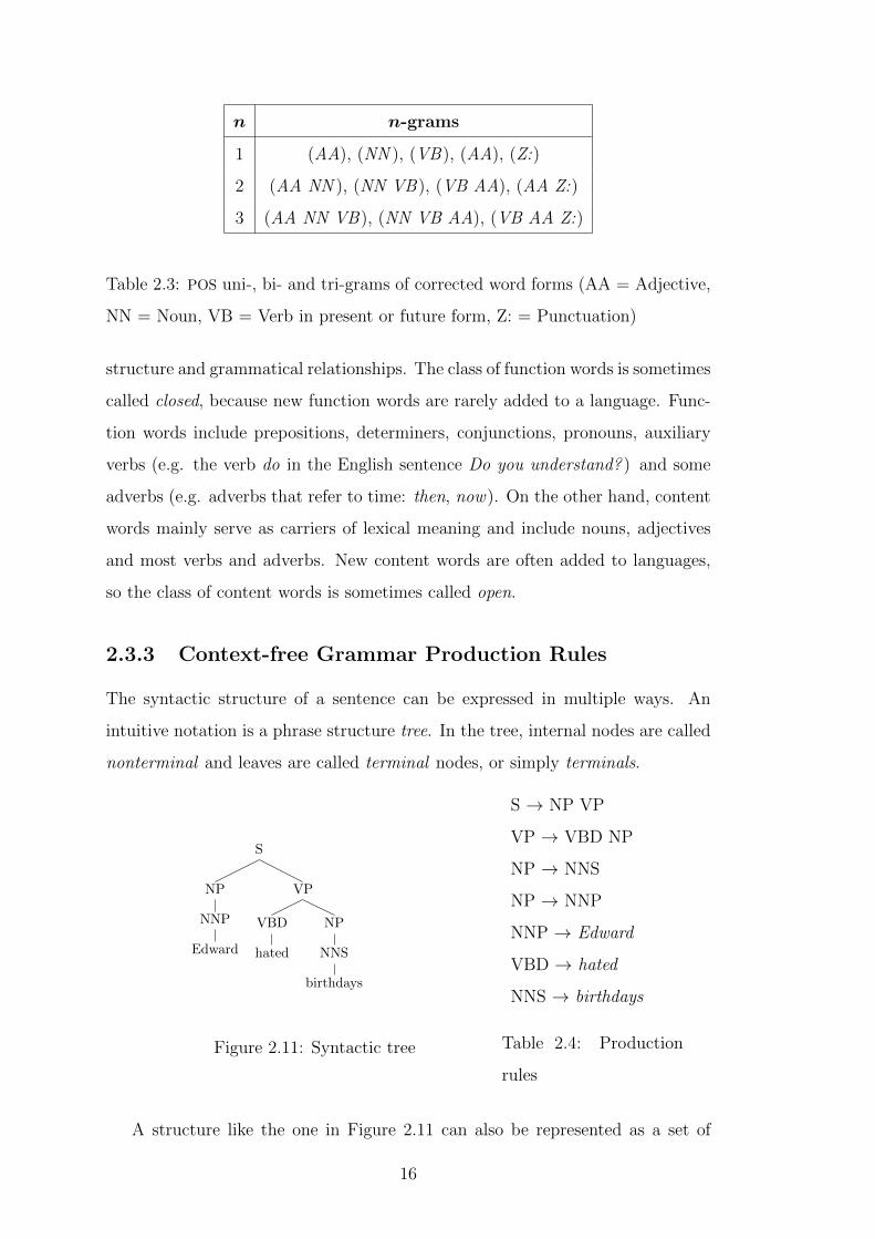
2.3.3 Context-free Grammar Production Rules

The syntactic structure of a sentence can be expressed in multiple ways. An

intuitive notation is a phrase structure tree. In the tree, internal nodes are called

nonterminal and leaves are called terminal nodes, or simply terminals.

S

NP

NNP

Edward

VP

VBD

hated

NP

NNS

birthdays

Figure 2.11: Syntactic tree

S → NP VP

VP → VBD NP

NP → NNS

NP → NNP

NNP → Edward

VBD → hated

NNS → birthdays

Table 2.4: Production

rules

A structure like the one in Figure 2.11 can also be represented as a set of

16

production rules (or rewrite rules) of the form X → Y1Y2 . . . Yn, where X is a

terminal symbol and Y1Y2 . . . Yn is a sequence of terminals and nonterminals:5

A context-free grammar G = (T,N, S,R) consists of a set of terminals T , a

set of nonterminals N , a start symbol S (which is a nonterminal) and a set of

production rules R of the form as shown in 2.4.

2.3.4 Errors

Apart from different patterns distributed in texts, corpora tagged for errors pro-

vide extra information. The motivation for using errors (typically represented by

a form of an error tag) comes from the assumption that errors that a learner of

a second language makes are related to his native language. Tagged errors may

include for example syntactic errors (i.e. subject-verb disagreement) or errors in

morphology (i.e. inflectional ending).

5NNP = Proper noun, singular; NNS = Noun, plural; VBD = Verb, past tense

17

18

3. Native Language Identification

Background

The general task of examining text in order to determine or verify characteristics

of the text’s author is commonly referred to as authorship attribution. The task

can be broadly defined on any piece of linguistic data (Juola [2006]), but we will

further on assume written text. Koppel et al. [2009] provide a detailed overview

of previous work in the area of statistical authorship attribution. In one of the

recognized scenarios, in the profiling problem, the aim is to provide as much

demographic or psychological information about the author as possible. This

information might include gender (Koppel et al. [2002]), age (Schler et al. [2006])

or even personality traits (Pennebaker et al. [2003]).

We consider the task of Native Language Identification to be an authorship

attribution problem of the profiling scenario. In recent years, serious achievements

in Native Language Identification (NLI) have been accomplished by treating the

task as a machine learning problem. Existing approaches differ in several ways:

First, most use English as the target language. But in the last few years, like

us, some (e.g. Aharodnik et al. [2013], Malmasi and Dras [2014a], Malmasi and

Dras [2014b]) have concentrated on other languages as well. Second, even when

working with one language, different corpora are being used, resulting in limited

comparability.1 Finally, a great variety of features are explored and implemented.

We keep these differences in mind throughout this section, which provides an

overview of previous work in the area of NLI.

3.1 English NLI

The first work focusing on identifying native language from text was done by

Koppel et al. [2005], who used data from the International Corpus of Learner

English (ICLE) (Granger et al. [2002]). The corpus consists of essays written by

1Tetreault et al. [2012] suggest that proficiency reporting would help in comparing results

across different corpora.

19

university students of the same English proficiency level. The authors classified a

sample of essays into 5 classes by the students’ native language: Czech, Bulgarian,

Russian, French and Spanish. They achieved an accuracy of 80.2% with the

20% baseline using function words, character n-grams, error types and rare (less

frequent) POS bigrams as features. Feature values are computed as frequencies

relative to document length. Orthographic errors were found in texts by the

MS Word spell checker and then assigned a type by a separate tool. Focusing on

these, the authors explore and find some distinctive patterns useful for identifying

native speakers of particular languages – for example, native speakers of Spanish

tended to confuse m and n (confortable) or q and c (cuantity, cuality).

The ICLE has been a popular choice for many others. See Table 3.2 for a

categorization by corpora and classification algorithms. We will now distinguish

previous experiments by feature types used.

3.1.1 Feature Types

– Syntactic features : Wong and Dras [2009] replicate the work of Koppel

et al. [2005] on the second version of the ICLE (Granger et al. [2009],

ICLEv2) choosing the same five languages and adding Chinese and Japanese.

They explore the role of three syntactic error types as features. The errors

(subject-verb disagreement, noun-number disagreement and determiner dis-

use) are detected by a grammar checker, Queequeg.2 Classification with

these three features (represented as relative frequencies) alone gives an ac-

curacy of about 24%. However, combining the features used by Koppel

et al. [2005] with the three syntactic errors types does not lead to any

improvement in accuracy, sometimes even causing accuracy decrease.

Syntactic features are further evaluated on the same data set (7 languages

from the second version of the ICLE) by Wong and Dras [2011]. They

introduce sets of context-free grammar (CFG) production rules as binary

features. The rules are extracted using the Stanford parser (Klein and Man-

ning [2003]) and the Charniak and Johnson parser (Charniak and Johnson

2http://queequeg.sourceforge.net/index-e.html

20

[2005]) and tested in two settings, lexicalised3 with function words and

punctuation and non-lexicalised.

Bykh and Meurers [2014] follow this approach by also concentrating on

CFG rule features for the task of NLI. They consider and systematically ex-

plore both non-lexicalized and lexicalized CFG features, experimenting with

different feature representations (binary values, normalized frequencies).

They define three feature types: phrasal CFG production rules excluding

all terminals (e.g. S → NP), lexicalized CFG production rules of the type

preterminal → terminal (e.g. JJ → nice) and the union of these two. The

obtained results vary greatly when comparing single-corpus (best reported

results of 78.8%) and cross-corpus (best reported results of 38.8%) settings,

confirming the challenge of achieving high cross-corpus results in the task

of NLI.

– Apart from syntactic features, the significance of using character, word or

POS n-grams when dealing with the task of NLI has been addressed by

several authors:

Tsur and Rappoport [2007] also follow Koppel et al. [2005] by choosing the

same five languages4 from the ICLE. Forming a hypothesis that the choice of

words people make when writing in a second language is influenced by the

phonology of their native language, they focus on character n-grams with

an emphasis on bigrams. By selecting 200 most frequent bigrams in the

whole corpus, an accuracy of 65.6% is achieved. Repeating the experiment

with 200 most frequent trigrams yields an accuracy of 59.7%.

Bykh and Meurers [2012] introduce classes of recurring n-grams (n-grams

that occur in at least two different essays of the training set) of various

lengths as features in their experiment. Three feature classes are described:

word-based n-grams (the surface forms), POS-based n-grams (all words are

3A non-terminal is annotated with its lexical head (a single word). For example, the rule

VP→VBD NP PP could be replaced with a rule such as VP(dumped) → VBD(dumped)

NP(sacks) PP(into) (example from Martin and Jurafsky [2000]).

4Bulgarian, Czech, French, Russian, Spanish

21

n = 1 n = 2

Word-based n-grams (analyzing), (attended) (aspect of ), (could only)

POS-based n-grams (NNP), (MD) (NNS MD), (NN RBS )

Open-Class-POS-based n-grams (far), (VBZ ) (NN whenever), (JJ well)

Table 3.1: Examples of features used by Bykh and Meurers [2012].

converted to the corresponding POS tags) and Open-Class-POS-based n-

grams (n-grams, where nouns, verbs, adjectives and cardinal numbers are

replaced by corresponding POS tags). See Table 3.1 for examples of these

feature classes. Essays are represented as binary feature vectors. Exper-

iments included both single n (unigrams, bigrams etc.) and [1-n] n-gram

(uni-grams, uni- and bigrams, uni-, bi- and trigrams etc.) settings. Without

discarding any features, Bykh and Meurers [2012] confirm satisfying results

for word [1-2]-gram features with accuracy nearly 90%, and for Open-Class-

POS-based [1-3]-grams (80.6%).

– Function words : Further replicating the work of Koppel et al. [2005], Tsur

and Rappoport [2007] test the performance of function word based features.

Relative frequencies of 460 English function words give 66.7% accuracy.

Function words are also employed by Brooke and Hirst [2011], Brooke and

Hirst [2012], Tetreault et al. [2012] and others.

Kochmar [2011] uses a subset of the Cambridge Learner Corpus (CLC)5 and

investigates binary classification of related Indo-European language pairs (e.g.

Spanish-Catalan, Danish-Swedish). This work presents a systematic study of

various feature groups and their contribution to overall classification results.

Employed features include POS n-grams, character n-grams and phrase struc-

ture rules. Unlike most of other studies, which use the Penn Treebank tagset,

Kochmar [2011] uses the CLAWS tagset.6 Apart from the mentioned features,

the author also concentrates on an error-based analysis, examining error type

5http://www.cambridge.org/us/cambridgeenglish/about-cambridge-english/

cambridge-english-corpus

6http://ucrel.lancs.ac.uk/claws/

22

rates (normalized by text length), error type distribution (normalized by num-

ber of error types in text) and error content (error codes are associated with the

incorrect word forms).

Author(s) Data Algorithm

Koppel et al. [2005] ICLE SVM

Tsur and Rappoport [2007] ICLE SVM

Wong and Dras [2009] ICLEv2 SVM

Wong and Dras [2011] ICLEv2 MaxEnt

Brooke and Hirst [2011] ICLEv2, Lang-8 SVM

Kochmar [2011] CLC SVM

Brooke and Hirst [2012] ICLEv2, Lang-8, CLC MaxEnt, SVM

Tetreault et al. [2012] ICLE-NLI, TOEFL7, TOEFL11, TOEFL11-Big Logistic regression

Bykh and Meurers [2012] ICLEv2 SVM

Bykh and Meurers [2014] TOEFL11, NT11 Logistic regression

Table 3.2: Summary of previous work – corpora and algorithms

3.1.2 Cross-corpus evaluation

Some researchers test generalizability of their results. For example, Bykh and

Meurers [2012] conducted a second set of experiments, using ICLE data for train-

ing and a set of other corpora (Non-Native Corpus of English,7 Uppsala Student

English Corpus8 and Hong Kong University of Science and Technology English

Examination Corpus9) for testing. The results obtained in a cross-corpus evalu-

ation vary from 86.2% (Open-Class-POS n-grams) to 87.6% (surface-based word

n-grams), suggesting, that the features introduced by using the ICLE generalize

well to other corpora.

A previous study though, by Brooke and Hirst [2011], states quite the opposite

and criticizes the usage of the ICLE for the task of Native Language Identification.

The authors test their claim that topic bias plays a major role during classification

using ICLE:

7essays written by Spanish native speakers

8essays written by Swedish native speakers

9essays written by Chinese native speakers

23

They infer this from an experiment which compares classification performance

on randomly split and topic-based split data. For example, when using character

n-grams, randomized split performance is more than 80%, whereas only 50% is

achieved with a topic based split. Brooke and Hirst [2011] introduce Lang-8,

an alternative web-scraped corpus. Data is derived from the Lang-8 website,10

which contains journal entries by language learners, which are corrected by native

speakers.

Brooke and Hirst [2012] further explore cross-corpus evaluation using Lang-8

as the training corpus and the ICLE and a sample of the CLC for testing. Three

experiments are evaluated: distinguishing between 7 languages11, between 5 Eu-

ropean languages and between Chinese and Japanese.

3.1.3 Native Language Identification Shared Task 2013

In 2013, a NLI shared task12 was organised, addressing goals of NLI community

unification and field progression. The 29 participating teams gained access to

the TOEFL11 corpus (Blanchard et al. [2013]), which consists of 1100 essays per

language, covering 11 languages. The essays were collected through the college

entrance Test of English as a Foreign Language (TOEFL) test delivery system of

the Educational Testing Service (ETS). Tetreault et al. [2013] provide a compre-

hensive overview of the results of the shared task. The shared task consisted of

three sub-tasks, differing in the training data used. The main subtask restricted

training data to TOEFL11-TRAIN, a specified subset of TOEFL11. Following prior

work (Koppel et al. [2005], Wong and Dras [2009] etc.), a majority of the teams

used Support Vector Machines (SVMs).

The most common features were word, character and POS n-grams (see Table

3.3), typically ranging from unigrams to trigrams. However for example Jarvis

et al. [2013] tested usage of character n-grams with n as high as 9 and reports

levels of accuracy nearly as high when using a model based on character n-grams

as the winning model involving lexical and part-of-speech n-grams.

10http://lang-8.com

11Polish, Russian, French, Spanish, Italian, Chinese, Japanese

12See https://sites.google.com/site/nlisharedtask2013/home for more details

24

Team Name

Abbreviation

Overall

AccuracyLearning Method Feature Types

JAR 84% SVM word, POS and character n-grams

OSL 83% word and character n-grams

BUC 83% Kernel Ridge Regression character-based

CAR 83% Ensemble word, POS and character n-grams

TUE 82% SVM word and POS n-grams, syntactic features

NRC 82% SVM word, POS and character n-grams, syntactic features

HAI 82% Logistic Regression POS and character n-grams, spelling features

CN 81% SVM word, POS and character n-grams, spelling features

NAI 81% word, POS and character n-grams, syntactic features

UTD 81%

Table 3.3: An overview of features and learning methods used by the top 10

teams in the NLI Shared Task. Based on Tables 3, 7 and 8 from Tetreault et al.

[2013]

Popescu and Ionescu [2013] submitted a model based solely on character-level

features, treating texts as sequences of symbols. Their system made use of string

kernels and a biology-inspired kernel.

Hladka et al. [2013] distinguish between n-grams of words and n-grams of

lemmas (base forms of words) and also introduce two types of skipgrams of words:

– First, for a sequence of words wi−3, wi−2, wi−1, wi, bigram (wi−2, wi) and

trigrams (wi−3, wi−1, wi), (wi−3, wi−2, wi) are extracted (Type 1).

– Second, for a sequence of words wi−4, wi−3, wi−2, wi−1, wi, bigrams (wi−3, wi),

(wi−4, wi) and trigrams (wi−4, wi−3, wi), (wi−4, wi−2, wi) and (wi−4, wi−1, wi)

are extracted (Type 2).

See the following example sentence:13

wi−4 wi−3 wi−2 wi−1 wi

Ja bych koupila sobe auto

I would buy myself a car

13Example sentence from the Cze-SLT corpus (Sebesta et al. [2014]).

25

n = 2 n = 3

Type 1 (koupila, auto) (bych, sobe, auto), (bych, koupila, auto)

Type 2 (bych, auto), (Ja, auto) (Ja, bych, auto), (Ja, koupila, auto), (Ja, sobe, auto)

Table 3.4: Skipgrams of example sentence

These skipgrams are in line with the definition in Guthrie et al. [2006], with the

difference, that 0-skip n-grams are not considered, as they are already represented

in the feature class of word n-grams.

Malmasi et al. [2013] propose function word n-grams as a novel feature. Func-

tion word n-grams are defined as a type of word n-grams, where content words

are skipped. The example that the authors present is the following: the sentence

We should all start taking the bus would be first stripped of content words and

reduced to we should all the, from which n-grams would be extracted.

Syntactic features (previously evaluated by Wong and Dras [2009] and Wong

and Dras [2011]) were used by six teams, though all of them combined these with

word, character or POS n-grams and it is thus hard to say how big the role the

syntactic features played. For example, Malmasi et al. [2013] implemented Tree

Substitution Grammar (TSG) fragments and Stanford dependencies14 (following

Tetreault et al. [2012]) as features.

3.2 non-English NLI

The majority of experiments have been carried out using texts written in English,

with various native language (L1) background of the authors. Recently, like we

do, some researchers have also focused on non-English second languages: Czech,

Chinese, Arabic, Finnish and Norwegian. We provide a summary of their work.

One has to take into account that these results are even less comparable, but

14Counts of basic dependencies extracted using the Stanford Parser (http://nlp.stanford.

edu/software/stanford-dependencies.shtml). An example from De Marneffe and Manning

[2008]: considering the sentence Sam ate 3 sheep, one of the extracted grammatical relations

would be a numeric modifier (any number phrase that serves to modify the meaning of the

noun with a quantity), represented as num(sheep, 3).

26

serve well when validating language independent methods. For a brief overview,

see Table 3.5.

Author(s) LanguageLearning

MethodFeature Types

Aharodnik et al. [2013] Czech SVM POS n-grams, error types

Malmasi and Dras [2014b] Chinese SVM POS n-grams, function words, CFG production rules

Wang and Yamana [2016] Chinese SVMPOS, character and word n-grams, function words,

CFG production rules, skip-grams

Malmasi and Dras [2014a] Arabic SVM POS n-grams, function words, CFG production rules

Malmasi and Dras [2014c] Finnish SVM POS and character n-grams, function words

Malmasi et al. [2015a] Norwegian SVMPOS n-grams, mixed POS-function word n-grams,

function words

Table 3.5: Summary of previous work – non-English data

3.2.1 Czech

To our knowledge the only previous work in NLI which focused on Czech as the

target language was conducted by Aharodnik et al. [2013], who work with data

which formed the basis for the CzeSL-SGT corpus used by us.15 Using about

1400 essays from the Czech as a Second Language (CzeSL) corpus (Hana et al.

[2010]), the authors classify Czech texts into two classes, determining whether the

L1 of the author belongs to the Indo-European or non-Indo-European language

group. This work is the closest related to our experiment.

As their primary goal, they focus on using only non-content based features

to avoid corpus specific dependency. These consist of a set of 264 POS bi-grams

and 305 tri-grams (with 3 or more occurrences in the data) and 35 extracted

error types. The authors use a SVM classifier and represent feature values as

term weights S, which are computed as a rounded logarithmic ratio of the token i

frequency in document j to the total amount of tokens in the document ([Manning

and Schutze, 1999, p.580]):

Sij = round

(10× 1 + log(tfij)

1 + log(lj)

)(3.1)

15See Section 4.1.2

27

A combination of all three types of features (errors and POS n-grams) yields a

promising performance of 85% precision and 89% recall. Errors alone also perform

well at 84% precision and recall. Results distinguishing performance on different

levels of author proficiency are provided.

3.2.2 Chinese

The first to develop a NLI system for Chinese, Malmasi and Dras [2014b] com-

bine sentences from the same L1 to manually form documents for classification,

as full texts are not available in the Chinese Learner Corpus (Wang et al. [2012]).

3.75 million tokens of text are extracted. The authors use 11 classes, some (Ko-

rean, Spanish, Japanese) overlapping with the languages of the TOEFL11 corpus,

which was previously used in the NLI Shared Task. Due to the fact that the

Chinese Learner Corpus is not topic-balanced, the authors avoid topic-dependent

lexical features such as character or word n-grams. Experiments are run with

both binary and normalized features and results indicate normalized features to

be more informative (in contrast, Brooke and Hirst [2012] make an opposite find-

ing for English NLI). By combining all features, that is POS n-grams (n = 1,2,3),

function words and CFG production rules, the highest achieved accuracy is 70.6%.

Wang and Yamana [2016] use the Jinan Chinese Learner Corpus (Wang et al.

[2015]), which mainly consists of essays written by speakers of languages of Asia

(most frequently Indonesian: 39% of essays, Thai: 15% and Vietnamese: 9%).

Adopted features include character, word and POS n-grams, function words, CFG

production rules and 1-skip bigrams (based on Guthrie et al. [2006]): for a se-

quence of words

wi−4, wi−3, wi−2, wi−1, wi

bigrams (wn−1, wn), (wn−2, wn) are extracted, here we would obtain 7 bigrams and

n would range from i to i − 3. For example, from the sentence Ja bych koupila

sobe auto, bigrams (Ja, bych), (bych, koupila), (koupila, sobe), (sobe, auto), (Ja,

koupila), (bych, sobe) and (koupila, auto) would be extracted.

Wang and Yamana [2016] achieve an average accuracy of 75.3%, with highest

scores for essays written by speakers of Thai (84.5%) and lowest for speakers of

Mongolian (33.6%). The authors consider low performance to be a consequence

28

●

●

●

●

●

●

●

●

●

●

0 2 4 6 8

0.0

0.2

0.4

0.6

0.8

log(# of training essays)

Acc

urac

y

IND

THA

VIEKOR

BUR

LAO

KHM

FIL

JAP

MON

Figure 3.1

of insufficient size of training data. The relationship between training data size

and classification accuracy is illustrated in Figure 3.1.

3.2.3 Arabic

Malmasi and Dras [2014a] work with a subset of the second version of the Ara-

bic Learner Corpus (ALC),16 which contains texts by Arabic learners studying in

Saudi Arabia. The subset used for experiments consists of 329 essays of speak-

ers with 7 different native language backgrounds. Given the topic imbalance of

the ALC, the authors choose to avoid lexical features and concentrate on three

syntactic feature types: CFG production rules, Arabic function words and POS n-

grams. For single feature type settings, POS bigrams performed best. All features

combined provided an accuracy of 41%.

3.2.4 Finnish

Malmasi and Dras [2014c] use a subset of 204 documents from the Corpus of

Advanced Learner Finnish (Ivaska [2014]). Function words, POS n-grams of size

1-3 and character n-grams up to n=4 are used as features. The authors use a

16http://www.arabiclearnercorpus.com/

29

majority baseline of 19.6% and report an accuracy of 69.5% using a combination

of all features. A second experiment is conducted for distinguishing non-native

writing, achieving 97% accuracy using a 50% chance baseline. Here all features

score 88% or higher.

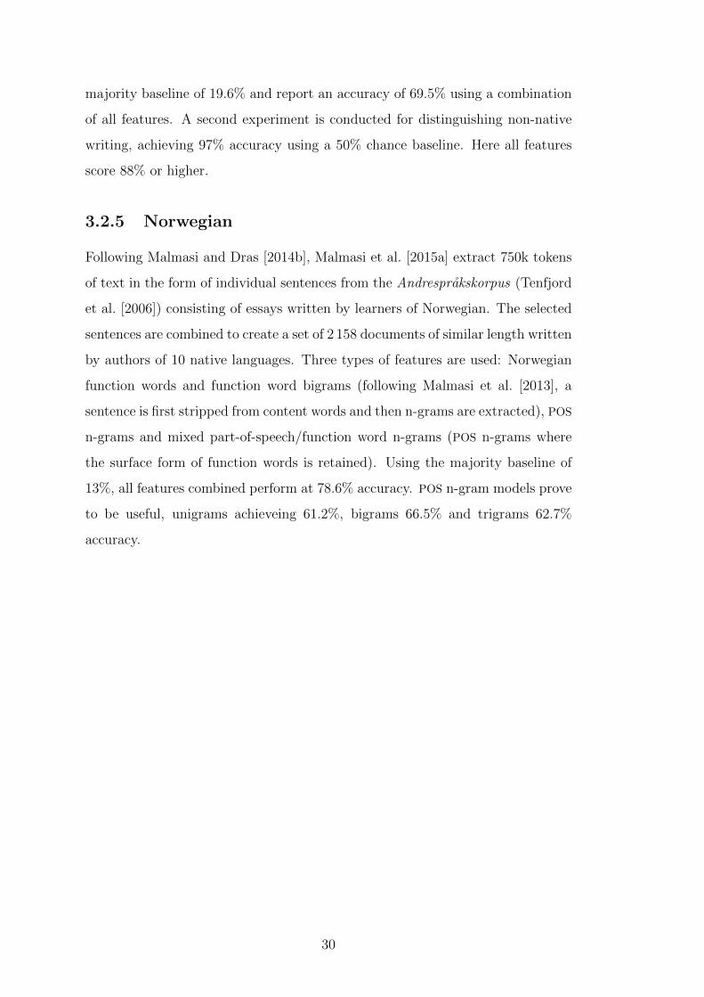
3.2.5 Norwegian

Following Malmasi and Dras [2014b], Malmasi et al. [2015a] extract 750k tokens

of text in the form of individual sentences from the Andresprakskorpus (Tenfjord

et al. [2006]) consisting of essays written by learners of Norwegian. The selected

sentences are combined to create a set of 2 158 documents of similar length written

by authors of 10 native languages. Three types of features are used: Norwegian

function words and function word bigrams (following Malmasi et al. [2013], a

sentence is first stripped from content words and then n-grams are extracted), POS

n-grams and mixed part-of-speech/function word n-grams (POS n-grams where

the surface form of function words is retained). Using the majority baseline of

13%, all features combined perform at 78.6% accuracy. POS n-gram models prove

to be useful, unigrams achieveing 61.2%, bigrams 66.5% and trigrams 62.7%

accuracy.

30

4. Our work

4.1 Data

4.1.1 Czech Language

The Czech language is a member of the West Slavic family of languages.1 It is

spoken by over 10 million people, mainly in the Czech Republic.

Regarding morphology, Czech is highly inflected (words are modified to ex-

press different grammatical categories) and fusional (one morpheme form can

simultaneously express several different meanings).

4.1.2 Corpus

We use a subset of the publicly available Czech as a Second Language with

Spelling, Grammar and Tags (CzeSL-SGT, Sebesta et al. [2014]) corpus, which

was developed as an extension of a part of the CzeSL-plain (“plain” meaning not

annotated) corpus, adding texts collected in 2013. CzeSL-plain consists of three

parts, ciz (a subset of CzeSL-SGT), kval (academic texts obtained from non-

native speakers of Czech studying at Czech universities in masters or doctoral

programmes) and rom (transcripts of texts written at school by pupils and stu-

dents with Romani background in communities endangered by social exclusion).

ru zh uk ko en kk ja de es fr vi ar pl tr it

mn uz ky hu ro

Language

Cou

nt

010002000300040005000

Figure 4.1: Distribution of 20 most frequent languages in CzeSL-SGT

1Together with, for example, Slovak and Polish.

31

The corpus contains transcripts of essays of non-native speakers of Czech

written in 2009-2013. It originally contains 8,617 texts by 1,965 authors with 54

different first languages, Figure 4.1 shows their distribution.

The data cover several language levels of the Common European Framework

of Reference for Languages (CEFR),2 ranging from beginner (A1) to upper in-

termediate (B2) level and some higher proficiency. There are 862 different topics

in CzeSL-SGT, such as Moje rodina, Dopis kamaradce/kamaradovi, Nejhorsı den

meho zivota or Co se stane, az dojde ropa?.3 749 essays do not include a topic

specification.

Metadata information consists of 30 attributes, most of which are assigned

to each text. 15 of these attributes contain information about the texts and 15

contain information about the authors. A list of these attributes can be found in

Appendix A.

Annotation

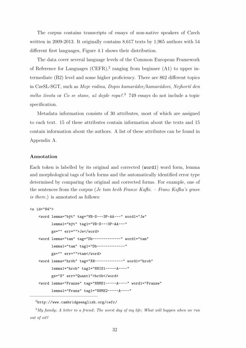
Each token is labelled by its original and corrected (word1) word form, lemma

and morphological tags of both forms and the automatically identified error type

determined by comparing the original and corrected forms. For example, one of

the sentences from the corpus (Je tam hrob Franze Kafki. – Franz Kafka’s grave

is there.) is annotated as follows:

<s id="84">

<word lemma="byt" tag="VB-S---3P-AA---" word1="Je"

lemma1="byt" tag1="VB-S---3P-AA---"

gs="" err="">Je</word>

<word lemma="tam" tag="Db-------------" word1="tam"

lemma1="tam" tag1="Db-------------"

gs="" err="">tam</word>

<word lemma="hrob" tag="X@-------------" word1="hrob"

lemma1="hrob" tag1="NNIS1-----A----"

gs="S" err="Quant1">hrob</word>

<word lemma="Franze" tag="NNMS1-----A----" word1="Franze"

lemma1="Franz" tag1="NNMS2-----A----"

2http://www.cambridgeenglish.org/cefr/

3My family ; A letter to a friend ; The worst day of my life; What will happen when we run

out of oil?

32

gs="" err="">Franze</word>

<word lemma="Kafki" tag="X@-------------" word1="Kafky"

lemma1="Kafka" tag1="NNMS2-----A----"

gs="S" err="Y0">Kafki</word>

<word lemma="." tag="Z:-------------" word1="."

lemma1="." tag1="Z:-------------"

gs="" err="">.</word>

</s>

Morphological tags of the Prague positional tagset (Hajic [2004]) are repre-

sented as a string of 15 symbols, each position corresponding to one morphological

category. Non-applicable values are denoted by a single hyphen (-). The 15 cat-

egories are described in Appendix B.

4.1.3 Our data

We excluded texts with unknown speaker IDs, unknown language group of first

language and texts where Czech was given as first language (possibly an error in

annotation). We also randomly selected 10% of all texts written by authors with

Russian as their first language, to acquire a better partitioning of languages and

language groups throughout the data.

Due to these operations, the number of texts we use is narrowed down to

3,715, with the distribution of authors’ first language groups as depicted in Table

4.1. The five most frequent languages are Chinese, Russian, Ukrainian, Korean

and English.

Language group Absolute count Relative count

non-Indo-European 1,747 47%

Slavic 1,070 29%

Indo-European 898 24%

All 3,715 100%

Table 4.1: Text counts by language groups

A great field of work in Native Language Identification (for English) has been

carried out on the TOEFL11 corpus (Blanchard et al. [2013]). It differs from CzeSL-

33

Absolute count Relative count

TRAIN 1,489 40%

DEV-TEST 1,115 30%

TEST 1,111 30%

All 3,715 100%

Table 4.2: Text counts by dataset split

SGT and the subset we use in several ways. First, TOEFL11 consists of 12,100

essays by native speakers of 11 languages (French, Italian, Spanish, German,

Hindi, Japanese, Korean, Turkish, Chinese, Arabic and Telugu). The essays are

equally distributed between the languages. In comparison, our subset of CzeSL-

SGT contains 3,715 Czech essays by native speakers of 52 languages, but the five

most frequent languages form about 50% of the dataset. Second, on average, 322

word tokens (at a range from two to 876) are contained in TOEFL11 essays. This

is almost three times more than texts in our CzeSL-SGT subset which contain

110 word tokens on average, at a range from 5 to 1,536. Third, CzeSL-SGT is

annotated for errors, which allows another whole area of NLI research. Finally,

only one essay per student is present in TOEFL11. In our data, each student

contributes by 2.9 essay on average and the number of essays per student range

from one to 22.

4.2 Tools

All of the scripts which extract features from text, filter features and prepare data

for classification are written in the Python programming language, version 2.7.4

Some of the figures are generated using the R language.5 We use the SVMlight

implementation of Support Vector Machines for classification.6

4https://www.python.org/

5https://www.r-project.org/

6http://svmlight.joachims.org/

34

4.3 Features

We employ six different feature types which are based on the distribution of

certain patterns in text: four n-gram types, function words and error types. Two

other features are average sentence and word length. We test four different values

for n-gram, function word and error feature types:

– Raw frequencies are simply the number of occurences of a pattern in a

document.

– Relative frequencies are raw frequencies of a pattern divided by the length

of the document.

– Log-normalized frequencies are computed as in Aharodnik et al. [2013]:

Sij = round

(10× 1 + log(tfij)

1 + log(lj)

)(4.1)

– Binary values denote only the fact that the pattern is present.

To distinguish between these value types, we use the following abbreviations:

raw, rel, log and bin.

4.3.1 n-grams

Character n-grams are extracted from individual words7 for n = 1, 2, 3. Before

extracting the n-grams, a word is converted to lowercase and padded from both

right and left with spaces, that is, a sequence of n− 1 spaces is appended to the

beginning and end of the word. This allows us to distinguish between a character

sequence that typically occurs in the middle of a word and the same sequence that

occurs more frequently at the end. Considering the word Je from the previously

introduced sentence and n = 2, we would extract bigrams ( , j ), (j, e), (e, ).

4.3.2 Function words

For our experiments, we extracted 300 most frequent function words from the

Prague Dependency Treebank (Bejcek et al. [2011]). We considered conjunctions,

7Here, we consider sequences of alphanumeric characters as words.

35

prepositions, particles and pronouns. When extracting feature values, we consider

only function words occurring at least twice in data.

4.3.3 Average length of word and sentence

We compute the average sentence length ls of document d as

ls(d) =

∑ni=1 |si|n

,

and the average word length lw(d) as

lw(d) =

∑ni=1 |wi|n

,

where n is the number of words and m is the number of sentences in d, considering

all sequences of alphabetical characters and digits as words.

4.3.4 Errors

Thanks to the annotation of errors in CzeSL-SGT, we are also able to conduct

an analysis based on the distribution of various error types in the essays. An

overview of all error types together with examples can be found in Appendix C.

4.4 Experiments on development data

At this point, we have chosen a set of feature types and a set of feature values.

Our task is now to explore the space of models that can be learned from our data

and choose such parameters and features, that the final model will have a good

ability of distinguishing texts written by Slavic and non-Slavic native speakers.

In this section, we give an overview of these initial experiments on development

data. In the next section, we give and analyze results on test data. Abbreviations

used to specify different types of kernel functions and feature types are described

in Tables 4.3 and 4.4.

For basic evaluation of a model’s performance, we use the F-score as a leading

measure. The F-score is defined as the harmonic mean of precision and recall:

F = 2 · precision · recallprecision+ recall

We now proceed in three steps, or runs:

36

Abbreviation Description

lin linear kernel function

poly-1 polynomial kernel function of degree 1

poly-2 polynomial kernel function of degree 2

poly-3 polynomial kernel function of degree 3

Table 4.3: Kernel functions

Abbreviation Description

CG[1-3] Character n-grams, n = 1, 2, 3

WG[1-3] Word n-grams, n = 1, 2, 3

PG[1-3] POS n-grams, n = 1, 2, 3

OG[1-3] Open-class-POS n-grams, n = 1, 2, 3

FW Function words

ER Error types

WL Word length

SL Sentence length

Table 4.4: Feature types

4.4.1 Run 1

The aims of the first run were to choose a value of the cost parameter C, which

influences the size of the hyperplane margin when classifying with SVMs,8 and the

types of kernel functions, each of which gives a different similarity measure.9

Table 4.5 shows the particular settings of run 1. We only tested individual

feature types (mainly because of time-saving reasons). We experimented with all

previously described feature values and various values of the cost parameter. As

kernel functions, we used both linear and polynomial functions, which have been

popular in previous work. We did not use the radial basis function, as it did not

prove useful in our preliminary experiments.

8See Section 2.1.2 for figures and details on how the cost parameter affects classification.

9See Equation 2.11 for a definition of the linear, polynomial and radial-basis kernel function.

37

Data DEV-TEST

Feature types CG[1-3], WG[1-3], PG[1-3], OG[1-3], ER, FW, WL, SL

Feature values bin, raw, rel, log

Kernels lin, poly-1, poly-2, poly-3

C parameter 0.001; 0.01; 0.1; 1.0; 10.0; 100.0; 1,000.0; 10,000.0

Information gain threshold 0

Table 4.5: Settings for run 1 of experiments.

Feature typeAll features

(count)

Selected features

(count)

Discarded features

(percentage)

CG[1-3] 9,710 9,003 7%

WG[1-3] 28,394 27,493 3%

PG[1-3] 6,260 5,862 6%

OG[1-3] 18,953 18,140 4%

ER 42 39 7%

FW 12 12 0%

All 63,371 60,549 4%

Table 4.6: Feature selection – run 1

Table 4.7 shows summary statistics of the experiments with common parame-

ters (type of kernel function and C parameter). It is sorted by the F-score mean.

We observed that the poly-3 kernel function performs significantly worse in both

F-score and accuracy, compared with lin, poly-1 and poly-2. We thus made

the choice not to include poly-3 in the next steps.

When considering the cost parameter C values, it is apparent (from Table 4.7)

that there is no clear lead. We fixed the value to 0.001 for all following experi-

ments, but we understand that more investigation would be needed for a robust

choice.

Table 4.6 shows how many features were discarded by selecting only features

with information gain larger than 0. The counts vary for the four possible feature

values, so the table contains the average of these. For example, 7,750 charac-

38

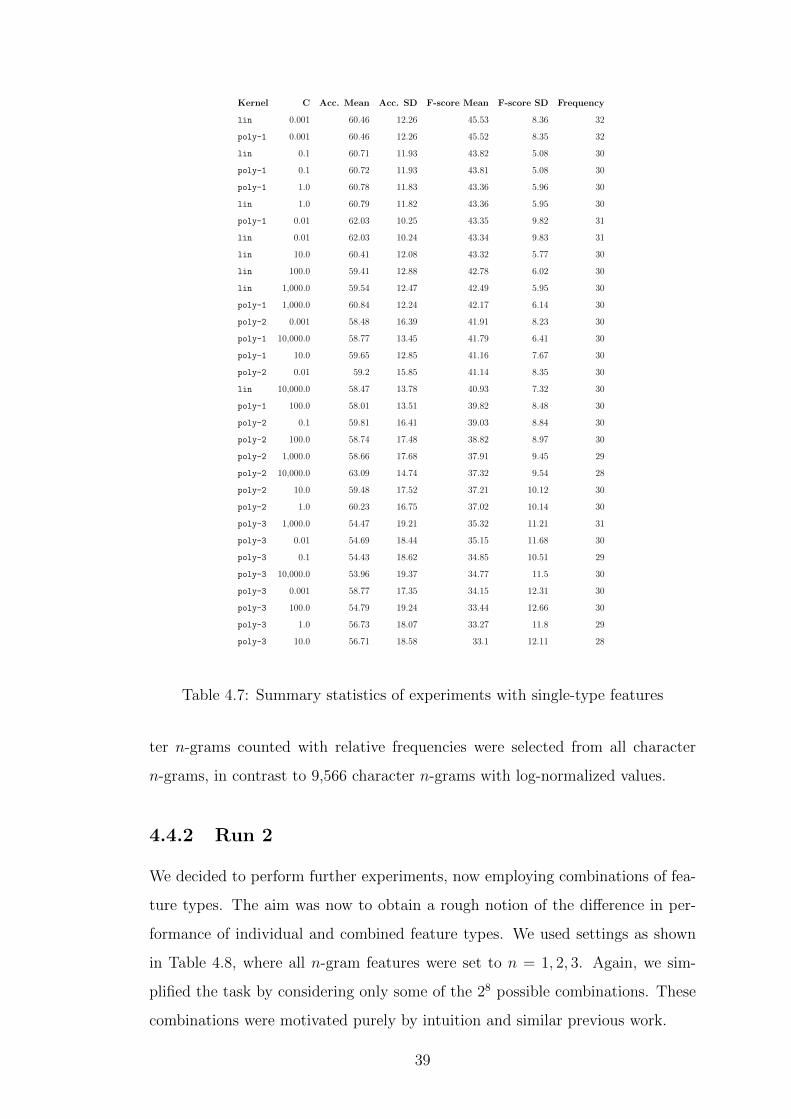
Kernel C Acc. Mean Acc. SD F-score Mean F-score SD Frequency

lin 0.001 60.46 12.26 45.53 8.36 32

poly-1 0.001 60.46 12.26 45.52 8.35 32

lin 0.1 60.71 11.93 43.82 5.08 30

poly-1 0.1 60.72 11.93 43.81 5.08 30

poly-1 1.0 60.78 11.83 43.36 5.96 30

lin 1.0 60.79 11.82 43.36 5.95 30

poly-1 0.01 62.03 10.25 43.35 9.82 31

lin 0.01 62.03 10.24 43.34 9.83 31

lin 10.0 60.41 12.08 43.32 5.77 30

lin 100.0 59.41 12.88 42.78 6.02 30

lin 1,000.0 59.54 12.47 42.49 5.95 30

poly-1 1,000.0 60.84 12.24 42.17 6.14 30

poly-2 0.001 58.48 16.39 41.91 8.23 30

poly-1 10,000.0 58.77 13.45 41.79 6.41 30

poly-1 10.0 59.65 12.85 41.16 7.67 30

poly-2 0.01 59.2 15.85 41.14 8.35 30

lin 10,000.0 58.47 13.78 40.93 7.32 30

poly-1 100.0 58.01 13.51 39.82 8.48 30

poly-2 0.1 59.81 16.41 39.03 8.84 30

poly-2 100.0 58.74 17.48 38.82 8.97 30

poly-2 1,000.0 58.66 17.68 37.91 9.45 29

poly-2 10,000.0 63.09 14.74 37.32 9.54 28

poly-2 10.0 59.48 17.52 37.21 10.12 30

poly-2 1.0 60.23 16.75 37.02 10.14 30

poly-3 1,000.0 54.47 19.21 35.32 11.21 31

poly-3 0.01 54.69 18.44 35.15 11.68 30

poly-3 0.1 54.43 18.62 34.85 10.51 29

poly-3 10,000.0 53.96 19.37 34.77 11.5 30

poly-3 0.001 58.77 17.35 34.15 12.31 30

poly-3 100.0 54.79 19.24 33.44 12.66 30

poly-3 1.0 56.73 18.07 33.27 11.8 29

poly-3 10.0 56.71 18.58 33.1 12.11 28

Table 4.7: Summary statistics of experiments with single-type features

ter n-grams counted with relative frequencies were selected from all character

n-grams, in contrast to 9,566 character n-grams with log-normalized values.

4.4.2 Run 2

We decided to perform further experiments, now employing combinations of fea-

ture types. The aim was now to obtain a rough notion of the difference in per-

formance of individual and combined feature types. We used settings as shown

in Table 4.8, where all n-gram features were set to n = 1, 2, 3. Again, we sim-

plified the task by considering only some of the 28 possible combinations. These

combinations were motivated purely by intuition and similar previous work.

39

Data DEV-TEST

Feature types

(CG, PG, OG), (CG, PG, WG, OG), (CG, PG, WG, OG, ER, FW),

(ER, FW), (PG, OG), (SL, WL), (SL, WL, PG, ER, FW),

(SL, WL, PG, FW), ALL

Feature values bin, raw, rel, log

Kernels lin, poly-1, poly-2

C parameter 0.001

Information gain threshold 0.001

Table 4.8: Settings for run 2 of experiments

Comparing some of the selected results in Appendices D and E indicates that

combining feature types is not always for the best. For example, both POS n-

grams and Open-Class POS n-grams perform over 70% accuracy on the average in

run 1, but combining them in run 2 leads to none or insignificant improvement.

Feature typeAll features

(count)

Selected features

(count)

Discarded features

(percentage)

CG, PG, OG 34,923 12,352 65%

CG, PG, OG, WG 63,317 19,737 69%

CG, PG, WG, OG, ER, FW 63,371 19,772 69%

ER, FW 54 35 35%

PG, OG 25,213 2,338 91%

SL, WL, PG, FW, ER 6,316 2,340 63%

SL, WL, PG, FW 6,274 2,340 63%

Table 4.9: Feature selection – run 2

4.4.3 Run 3

Regarding the plots of features with respect to their information gain (see Figures

4.2, 4.3 and Appendix G), we applied more strict feature selection, selecting

features with information gain larger than 0.002.

This was thus the third run of experiments, with settings as in run 2, but

combining feature types of both previous runs. Table F.1 shows selected results

for each feature group. As is obvious from Table 4.11, the number of features

40

0 2000 4000 6000 8000 10000

0.00

00.

005

0.01

00.

015

0.02

00.

025

Number of features

Info

rmat

ion

Gai

n

Figure 4.2: Character n-grams, log

0 5000 10000 15000 20000 25000

0.00

00.

002

0.00

40.

006

0.00

80.

010

0.01

20.

014

Number of features

Info

rmat

ion

Gai

n

Figure 4.3: Word n-grams, log

Data DEV-TEST

Feature types

CG[1-3], WG[1-3], PG[1-3], OG[1-3], ER, FW, WL, SL,

(CG, PG, OG), (CG, PG, WG, OG), (CG, PG, WG, OG, ER, FW),

(ER, FW), (PG, OG), (SL, WL), (SL, WL, PG, ER, FW),

(SL, WL, PG, FW), all

Feature values bin, raw, rel, log

Kernels lin, poly-1, poly-2

C parameter 0.001

Information gain threshold 0.002

Table 4.10: Settings for run 3 of experiments

dropped significantly by applying a strict information gain threshold. A drop,

though less notable, also occurred in nearly all results (measured by accuracy and

F-score), compared to both previous runs.

4.5 Results

For the final run and evaluation, we continued in employing the linear and poly-

nomial kernel functions and we also preserved the value of C, 0.001. Based on

development experiments, we made the choice to apply “liberal” feature selection

and only discarded features with zero information gain.

We decided to gain more details about the performance of n-gram features

41

Feature typeAll features

(count)

Selected features

(count)

Discarded features

(percentage)

CG[1-3] 9,710 2,210 77%

WG[1-3] 28,394 1,987 93%

PG[1-3] 6,260 1,068 83%

OG[1-3] 18,953 1,978 90%

ER 42 17 60%

FW 12 8 33%

All 63,371 7,243 89%

Table 4.11: Feature selection – run 3

and apart from feature groups as used in run 3, we also tested individual uni-,

bi- and tri-gram groups.

Each feature group was tested for different feature values and kernel functions,

and out of approximately 350 results that we obtained alltogether, 210 (60%)

performed at accuracy above the majority baseline of 67%.

For an overview of selected results, see Table 4.12 and Figure 4.4. Several

observations can be made:

– Considering n-gram features (character, word, POS and Open-Class POS

n-grams), a combination of all three n-gram types (n = 1, 2, 3) never out-

performed the best result of the individual groups.

– Binary and log-normalized values of features seem to dominate – 23 out of

28 best results consist of binary or log-normalized values. This is in line

with most of the previous work.

– n-gram features in general are useful and generate the highest accuracies

both on their own (character trigrams) and combined (character and OC-

POS n-grams).

– As expected, a closer look at word unigrams, which seem to produce sat-

isfying results, shows that topic bias is the main cause. When sorted by

42

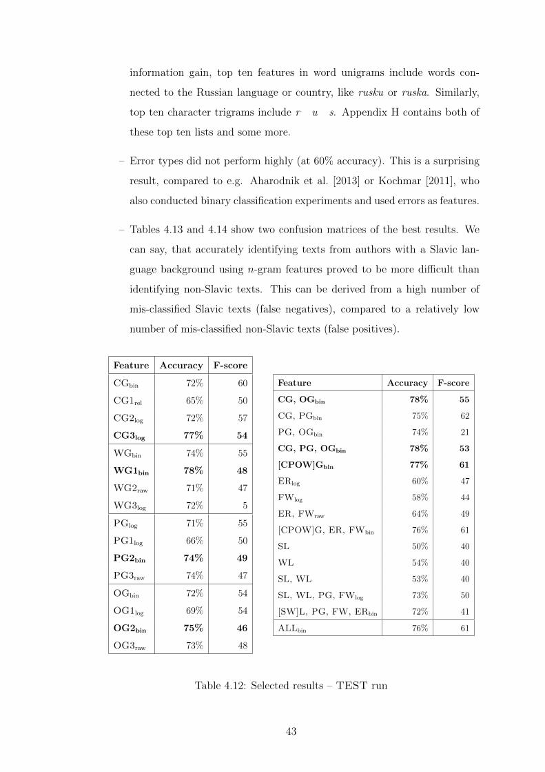
information gain, top ten features in word unigrams include words con-

nected to the Russian language or country, like rusku or ruska. Similarly,

top ten character trigrams include r u s. Appendix H contains both of

these top ten lists and some more.

– Error types did not perform highly (at 60% accuracy). This is a surprising

result, compared to e.g. Aharodnik et al. [2013] or Kochmar [2011], who

also conducted binary classification experiments and used errors as features.

– Tables 4.13 and 4.14 show two confusion matrices of the best results. We

can say, that accurately identifying texts from authors with a Slavic lan-

guage background using n-gram features proved to be more difficult than

identifying non-Slavic texts. This can be derived from a high number of

mis-classified Slavic texts (false negatives), compared to a relatively low

number of mis-classified non-Slavic texts (false positives).

Feature Accuracy F-score

CGbin 72% 60

CG1rel 65% 50

CG2log 72% 57

CG3log 77% 54

WGbin 74% 55

WG1bin 78% 48

WG2raw 71% 47

WG3log 72% 5

PGlog 71% 55

PG1log 66% 50

PG2bin 74% 49

PG3raw 74% 47

OGbin 72% 54

OG1log 69% 54

OG2bin 75% 46

OG3raw 73% 48

Feature Accuracy F-score

CG, OGbin 78% 55

CG, PGbin 75% 62

PG, OGbin 74% 21

CG, PG, OGbin 78% 53

[CPOW]Gbin 77% 61

ERlog 60% 47

FWlog 58% 44

ER, FWraw 64% 49

[CPOW]G, ER, FWbin 76% 61

SL 50% 40

WL 54% 40

SL, WL 53% 40

SL, WL, PG, FWlog 73% 50

[SW]L, PG, FW, ERbin 72% 41

ALLbin 76% 61

Table 4.12: Selected results – TEST run

43

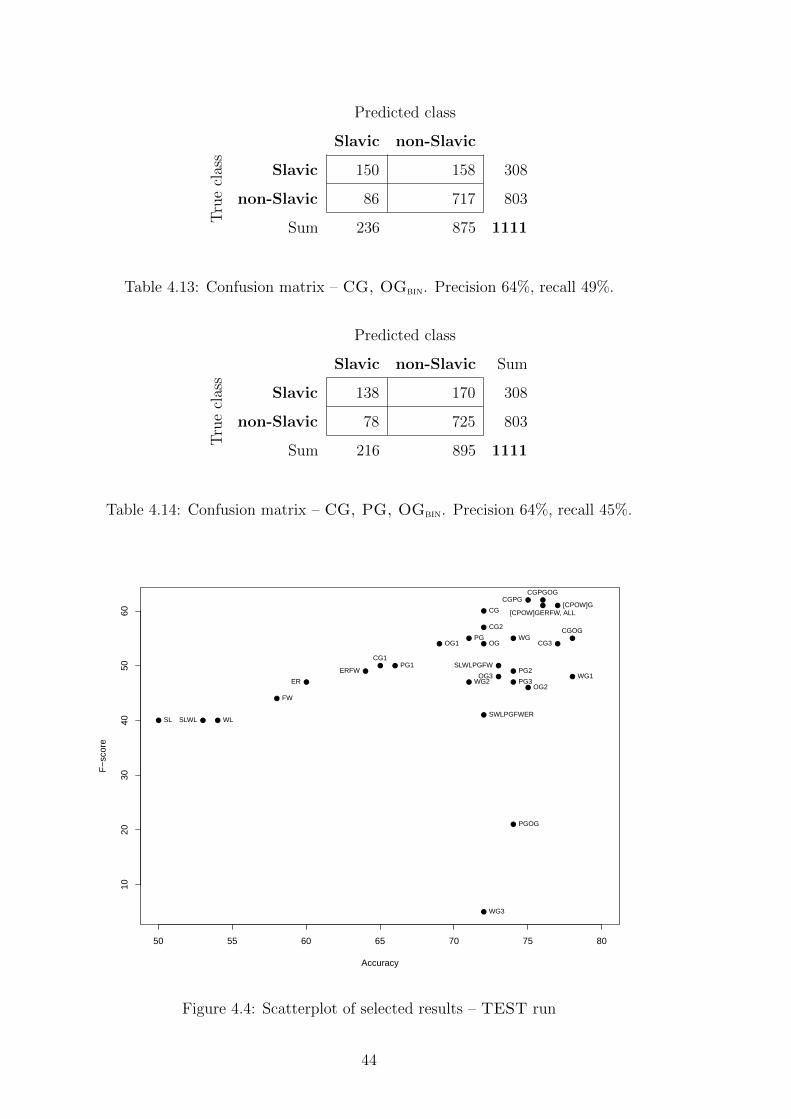
Predicted class

Slavic non-Slavic

Tru

ecl

ass

Slavic 150 158 308

non-Slavic 86 717 803

Sum 236 875 1111

Table 4.13: Confusion matrix – CG, OGbin. Precision 64%, recall 49%.

Predicted class

Slavic non-Slavic Sum

Tru

ecl

ass

Slavic 138 170 308

non-Slavic 78 725 803

Sum 216 895 1111

Table 4.14: Confusion matrix – CG, PG, OGbin. Precision 64%, recall 45%.

●

●

●

●●

●●

●

●

●●

●

●●

●

●

●

●

●

●●

●

●

●

● ●●

●

●

●

50 55 60 65 70 75 80

1020

3040

5060

Accuracy

F−

scor

e

CG

CG1

CG2

CG3WG

WG1WG2

WG3

PG

PG1PG2

PG3

OGOG1

OG2

OG3

CGOG

CGPG

PGOG

CGPGOG

[CPOW]G

ER

FW

ERFW

SL WLSLWL

SLWLPGFW

SWLPGFWER

[CPOW]GERFW, ALL

Figure 4.4: Scatterplot of selected results – TEST run

44

Conclusion

This thesis focused on the task of Native Language Identification (NLI) based on

Czech written text. Our main goal was to explore the possibilities of recogniz-

ing whether the author’s first language belongs to the Slavic language family or

not. Using the publicly available CzeSL-SGT corpus, we approached the task

as a binary classification machine learning problem and applied Support Vector

Machines as the learning method. We experimented with several kernel functions

and a variety of features and feature groups.

To our knowledge, this is the second work in the area of NLI addressing Czech

texts. The first, Aharodnik et al. [2013], focused on distinguishing Indo-European

and non-Indo-European native language background.

We have shown that Slavic and non-Slavic native languages can be told

apart with an accuracy up to 78% using character and Open-Class part-of-

speech (POS) n-grams. We have confirmed several results and hypotheses formed

in previous work, such as that binary values of features perform better than other

values (for instance relative frequencies), and that non-content features such as

POS n-grams, which provide the advantage of language independency, also give

satisfying results.

There are several directions in which future research can build upon and

improve our work. First, a finer exploration of parameters of the linear and

polynomial kernel could lead to better trained models. Next, grouping and re-

porting results by proficiency level would provide further insight into the limits

of our method; it could also contribute to comparability of results between cor-

pora in case of similar future research. Last, our task can be extended in a fairly

straightforward way towards identifying specific native languages.

45

46

Bibliography

Katsiaryna Aharodnik, Marco Chang, Anna Feldman, and Jirka Hana. Automatic

Identification of Learners’ Language Background based on their Writing in

Czech. In Proceedings of the 6th International Joint Conference on Natural

Language Processing (IJNCLP 2013), Nagoya, Japan, October 2013, pages

1428–1436, 2013.

Eduard Bejcek, Jan Hajic, Jarmila Panevova, Jirı Mırovsky, Johanka Spoustova,

Jan Stepanek, Pavel Stranak, Pavel Sidak, Pavlına Vimmrova, Eva St’astna,

Magda Sevcıkova, Lenka Smejkalova, Petr Homola, Jan Popelka, Marketa

Lopatkova, Lucie Hrabalova, Natalia Klyueva, and Zdenek Zabokrtsky. Prague

Dependency Treebank 2.5, 2011. URL http://hdl.handle.net/11858/00-

097C-0000-0006-DB11-8. LINDAT/CLARIN digital library at Institute of

Formal and Applied Linguistics, Charles University in Prague.

Daniel Blanchard, Joel Tetreault, Derrick Higgins, Aoife Cahill, and Martin

Chodorow. TOEFL11: A Corpus of Non-Native English. Technical report,

Educational Testing Service, 2013.

Julian Brooke and Graeme Hirst. Native language detection with ‘cheap’ learner

corpora. In Learner Corpus Research 2011, 2011.

Julian Brooke and Graeme Hirst. Robust, lexicalized native language identifica-

tion. In Proceedings of COLING 2012, 2012.

Serhiy Bykh and Detmar Meurers. Native Language Identification using Recur-

ring n-grams – Investigating Abstraction and Domain Dependence. In Proceed-

ings of COLING 2012, pages 425–440, 2012.

Serhiy Bykh and Detmar Meurers. Exploring Syntactic Features for Native Lan-

guage Identification: A Variationist Perspective on Feature Encoding and En-

semble Optimization. In COLING, pages 1962–1973, 2014.

Eugene Charniak and Mark Johnson. Coarse-to-fine n-best parsing and MaxEnt

discriminative reranking. In Proceedings of the 43rd Annual Meeting on Asso-

47

ciation for Computational Linguistics, pages 173–180. Association for Compu-

tational Linguistics, 2005.

Marie-Catherine De Marneffe and Christopher D. Manning. Stanford typed de-

pendencies manual. Technical report, Stanford University, 2008.

Sylviane Granger, Estelle Dagneaux, Fanny Meunier, et al. The International

Corpus of learner English. Handbook and CD-ROM. 2002.

Sylviane Granger, Estelle Dagneaux, Fanny Meunier, Magali Paquot, et al. The

International Corpus of learner English. Version 2. Handbook and CD-ROM.

2009.

David Guthrie, Ben Allison, Wei Liu, Louise Guthrie, and Yorick Wilks. A

Closer Look at Skip-gram Modelling. In Proceedings of the 5th International

Conference on Language Resources and Evaluation (LREC-2006), pages 1–4,

2006.

Jan Hajic. Disambiguation of Rich Inflection: Computational Morphology of

Czech. Karolinum, 2004.

Jirka Hana, Alexandr Rosen, Svatava Skodova, and Barbora Stindlova. Error-

tagged Learner Corpus of Czech. In Proceedings of the Fourth Linguistic An-

notation Workshop, pages 11–19. Association for Computational Linguistics,

2010.

Barbora Hladka, Martin Holub, and Vincent Krız. Feature Engineering in the NLI

Shared Task 2013: Charles University Submission Report. In 8th Workshop on

Innovative Use of NLP for Building Educational Applications, pages 232–241,

2013.

Ilmari Ivaska. The Corpus of Advanced Learner Finnish (LAS2): Database and

toolkit to study academic learner Finnish. Apples-Journal of Applied Language

Studies, 2014.

Scott Jarvis, Yves Bestgen, and Steve Pepper. Maximizing Classification Accu-

racy in Native Language Identification. In 8th Workshop on Innovative Use of

NLP for Building Educational Applications, 2013.

48

Patrick Juola. Authorship attribution. Foundations and Trends in information

Retrieval, 1(3):233–334, 2006.

Dan Klein and Christopher D. Manning. Accurate Unlexicalized Parsing. In

Proceedings of the 41st Annual Meeting on Association for Computational

Linguistics-Volume 1, pages 423–430. Association for Computational Linguis-

tics, 2003.

Ekaterina Kochmar. Identification of a Writer’s Native Language by Error Anal-

ysis. Master’s thesis, University of Cambridge, 2011.

Moshe Koppel, Shlomo Argamon, and Anat Rachel Shimoni. Automatically Cat-

egorizing Written Texts by Author Gender. Literary and Linguistic Computing,

17(4):401–412, 2002.

Moshe Koppel, Jonathan Schler, and Kfir Zigdon. Determining an Author’s

Native Language by Mining a Text for Errors. In Proceedings of the Eleventh

ACM SIGKDD International Conference on Knowledge Discovery and Data

Mining, pages 624–628. ACM, 2005.

Moshe Koppel, Jonathan Schler, and Shlomo Argamon. Computational Methods

in Authorship Attribution. Journal of the American Society for Information

Science and Technology, pages 9–26, 2009.

Shervin Malmasi and Mark Dras. Arabic Native Language Identification. In

Proceedings of the Arabic Natural Language Processing Workshop (EMNLP

2014), pages 180–186, 2014a.

Shervin Malmasi and Mark Dras. Chinese Native Language Identification. In

EACL, pages 95–99, 2014b.

Shervin Malmasi and Mark Dras. Finnish Native Language Identification. In

Proceedings of the Australasian Language Technology Workshop (ALTA), pages

139–144, 2014c.

Shervin Malmasi, Sze-Meng Jojo Wong, and Mark Dras. NLI Shared Task 2013:

MQ Submission. In 8th Workshop on Innovative Use of NLP for Building

Educational Applications, pages 124–133, 2013.

49

Shervin Malmasi, Mark Dras, and Irina Temnikova. Norwegian Native Language

Identification. Recent Advances in Natural Language Processing, pages 404–

412, 2015a.

Shervin Malmasi, Joel Tetreault, and Mark Dras. Oracle and Human Baselines

for Native Language Identification. In Proceedings of the Tenth Workshop on

Innovative Use of NLP for Building Educational Applications, pages 172–178,

2015b.

Christopher D Manning and Hinrich Schutze. Foundations of Statistical Natural

Language Processing. MIT Press, 1999.

James H Martin and Daniel Jurafsky. Speech and Language Processing. Inter-

national Edition, 2000.

James W Pennebaker, Matthias R Mehl, and Kate G Niederhoffer. Psychological

Aspects of Natural Language Use: Our Words, our Selves. Annual review of

psychology, 54(1):547–577, 2003.

Marius Popescu and Radu Tudor Ionescu. The Story of the Characters, the DNA

and the Native Language. In 8th Workshop on Innovative Use of NLP for

Building Educational Applications, pages 270–278, 2013.

Jonathan Schler, Moshe Koppel, Shlomo Argamon, and James W Pennebaker.

Effects of Age and Gender on Blogging. In AAAI Spring Symposium: Compu-

tational Approaches to Analyzing Weblogs, volume 6, pages 199–205, 2006.

Karel Sebesta, Zuzanna Bedrichova, Katerina Sormova, Barbora Stindlova, Mi-

lan Hrdlicka, Tereza Hrdlickova, Jirı Hana, Vladimır Petkevic, Tomas Jelınek,

Svatava Skodova, Marie Polackova, Petr Janes, Katerina Lundakova, Hana

Skoumalova, Simon Sladek, Piotr Pierscieniak, Dagmar Toufarova, Michal

Richter, Milan Straka, and Alexandr Rosen. AKCES 5 (CzeSL-CGT) Release

2, 2014. URL http://hdl.handle.net/11234/1-162. LINDAT/CLARIN dig-

ital library at Institute of Formal and Applied Linguistics, Charles University

in Prague.

50

Kari Tenfjord, Paul Meurer, and Knut Hofland. The ASK corpus: A Language

Learner Corpus of norwegian as a Second Language. In Proceedings of the

5th International Conference on Language Resources and Evaluation (LREC),

pages 1821–1824, 2006.

Joel Tetreault, Daniel Blanchard, and Aoife Cahill. A Report on the First Native

Language Identification Shared Task. In Proceedings of the eighth Workshop

on Innovative Use of NLP for Building Educational Applications, pages 48–57.

Association for Computational Linguistics, 2013.

Joel R Tetreault, Daniel Blanchard, Aoife Cahill, and Martin Chodorow. Native

Tongues, Lost and Found: Resources and Empirical Evaluations in Native

Language Identification. In COLING, pages 2585–2602, 2012.

Oren Tsur and Ari Rappoport. Using Classifier Features for Studying the Effect

of Native Language on the Choice of Written Second Language Words. In

Proceedings of the Workshop on Cognitive Aspects of Computational Language

Acquisition, pages 9–16. Association for Computational Linguistics, 2007.

Vladimir Naoumovitch Vapnik. Vosstanovlenie zavisimosteı po empiricheskim

dannym. Nauka, 1979.

Vladimir Naumovich Vapnik and Samuel Kotz. Estimation of dependences based

on empirical data, volume 40. Springer-Verlag New York, 1982.

Lan Wang and Hayato Yamana. Robust Chinese Native Language Identification

with Skip-gram. 2016.

Maolin Wang, Qi Gong, Jie Kuang, and Ziyu Xiong. The development of a

Chinese learner corpus. In International Conference on Speech Database and

Assessments, 2012.

Maolin Wang, Shervin Malmasi, and Mingxuan Huang. The Jinan Chinese

Learner Corpus. In Proceedings of the Tenth Workshop on Innovative Use

of NLP for Building Educational Applications, pages 118–123, 2015.

51

Sze-Meng Jojo Wong and Mark Dras. Contrastive Analysis and Native Lan-

guage Identification. In Proceedings of the Australasian Language Technology

Association Workshop, pages 53–61, 2009.

Sze-Meng Jojo Wong and Mark Dras. Exploiting Parse Structures for Native Lan-

guage Identification. In Proceedings of the Conference on Empirical Methods in

Natural Language Processing, pages 1600–1610. Association for Computational

Linguistics, 2011.

52

A. Czesl-SGT – Metadata

Type Value

t id

t date

t medium manuscript; typed

t limit minutes 10; 15; 20; 30; 40; 45; 60; other; none

t aid yes; dictionary; textbook; other; none

t exam yes; final; interim; n/a

t limit words 20; 20-; 25; 30; 35-; 40; 40-; 50; 50-; (. . . ); 200; 200-

t title

t topic type general; specific

t activity exercise; discussion; visual; vocabulary; other; none

t topic assigned multiple choice; specified; free; other

t genre assigned specified; free

t genre predominant informative; descriptive; argumentative; narrative

t words count

t words range -50; 50-99; 100-149; 150-199; 200-

Table A.1: Attributes of texts1

1The source of tables A.1 and A.2 is http://utkl.ff.cuni.cz/~rosen/public/meta_

attr_vals.html

53

Type Value

s id

s sex m; f

s age

s age cat 6-11; 12-15; 16-

s L1

s L1 group IE; nIE; S

s other langs

s cz CEF A1; A1+; A2; A2+; B1; B2; C1; C2

s cz in family 3; mother; father; partner; sibling; other; nobody

s years in CzR -1; 1; -2; 2-

s study cz 1to2; paid; TY (self-study); university; foreign; prim secondary; other

s study cz months -3; 3-6; 6-12; 12-24; 24-36; 36-48; 48-60; 60-

s study cz hrs week -3; 5-15; 15-

s textbook BC; CC; CE; CMC; CpC; ECE; NCSS; other

s bilingual yes; no

Table A.2: Attributes of authors

An example of metadata:

<div t_id="UJA2_8S_008" t_date="2011-06-17"

t_medium="manuscript" t_limit_minutes="45"

t_aid="none" t_exam="yes"

t_limit_words="150" t_title="Ceske silnice"

t_topic_type="general" t_activity=""

t_topic_assigned="multiple choice" t_genre_assigned="specified"

t_genre_predominant="argumentative" t_words_count="231"

t_words_range="200-"

s_id="UJA2_8S" s_sex="f"

s_age="18" s_age_cat="16-"

s_L1="en" s_L1_group="IE"

s_other_langs="" s_cz_CEF="A2"

s_cz_in_family="" s_years_in_CzR=""

s_study_cz="university" s_study_cz_months="6-12"

s_study_cz_hrs_week="15-" s_textbook="other"

s_bilingual="no">

54

B. Prague Positional Tagset

No. Name Description

1 POS Part of Speech

2 SUBPOS Detailed Part of Speech

3 GENDER Gender

4 NUMBER Number

5 CASE Case

6 POSSGENDER Possessor’s Gender

7 POSSNUMBER Possessor’s Number

8 PERSON Person

9 TENSE Tense

10 GRADE Degree of comparison

11 NEGATION Negation

12 VOICE Voice

13 RESERVE1 Unused

14 RESERVE2 Unused

15 VAR Variant, Style, Register, Special Usage

Table B.1: Morphological categories described by the Prague Positional Tagset

55

56

C. CzeSL-SGT – Errors

Error Type Error Description Examples

Cap0 capitalization: incorrect lower case evrope/Evrope; stedry/Stedry

Cap1 capitalization: incorrect upper case Stare/stare; Rodine/rodine

Caron0 error in diacritics – missing caron vecı/vecı; sobe/sobe

Caron1 error in diacritics – extra caron brecel/brecel; bratrem/bratrem

DiaE error in diacritics – e/e, e/e usmevave/usmevave; poprve/poprve

DiaU error in diacritics – u/u, u/u nemuzes/nemuzes; ukoly/ukoly

Dtn error in de/te/ne, di/ti/ni nikdo/nikdo; jest’erka/jesterka

Quant0 error in diacritics – missing vowel accent vzpominam/vzpomınam; doufam/doufam

Quant1 error in diacritics – extra vowel accent ktera/ktera; hledat/hledat

Voiced0 voicing assimilation: incorrectly voiceless stratıme/ztratıme; nabıtku/nabıdku;

Voiced1 voicing assimilation: incorrectly voiced zbalit/sbalit; nigdo/nikdo;

VoicedFin0 word-final voicing: incorrectly voiceless Kdys/Kdyz; vztach/vztah

VoicedFin1 word-final voicing: incorrectly voiced prez/pres; pag/pak

Voiced voicing: other errors pezky/pesky; hodili/chodili

Y0 i instead of correct y prazskıch/prazskych; vipije/vypije

Y1 y instead of correct i hlavnym/hlavnım; lıbyl/lıbil

YJ0 y instead of j yake/jake; yazykem/jazykem

CK0 c instead of correct k, except for palatalization Atlantic/Atlantik

Palat0 missing palatalization (k, g, h, ch) amerike/Americe; matke/matce

EpentE0 e epenthesis (missing e) najdnou/najednou; domcek/domecek

EpentE1 e epenthesis (extra e) rozebehl/rozbehl; ucety/ucty

EpentJ0 missing j after i before vowel napie/napije

EpentJ1 extra j after i before vowel dijamant/diamant

Gemin0 character doubling: missed doubling polostrove/poloostrove;

Gemin1 character doubling: extra doubling essej/esej; professor/profesor

Je0 e instead of correct je ubjehlo/ubehlo; Nejvjetsı/Nejvetsı

Je1 je instead of correct e vjedel/vedel; vjeci/veci

Mne0 chyba me instead of correct mne zapomela/zapomnela

Mne1 mne, mne or mne instead of correct me mnela/mela; rozumneli/rozumeli

ProtJ0 prothetic j: missing j sem/jsem; menoval/jmenoval

ProtJ1 prothetic j: extra j jse/se; jme/me

Meta metathesis (switching order of adjacent characters) dobrodruztsvı/dobrodruzstvı

Table C.1: Errors specified in detail1

1The source of tables C.1, C.2 and C.3 is http://utkl.ff.cuni.cz/~rosen/public/

SeznamAutoChybR0R1_en.html.

57

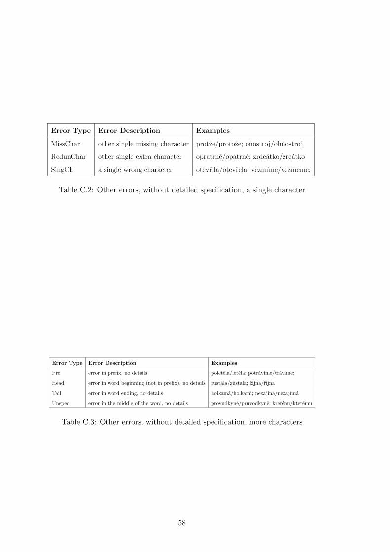
Error Type Error Description Examples

MissChar other single missing character protze/protoze; onostroj/ohnostroj

RedunChar other single extra character opratrne/opatrne; zrdcatko/zrcatko

SingCh a single wrong character otevrila/otevrela; vezmıme/vezmeme;

Table C.2: Other errors, without detailed specification, a single character

Error Type Error Description Examples

Pre error in prefix, no details poletela/letela; potravıme/travıme;

Head error in word beginning (not in prefix), no details rustala/zustala; zijna/rıjna

Tail error in word ending, no details holkama/holkami; nezajına/nezajıma

Unspec error in the middle of the word, no details provudkyne/pruvodkyne; krerenu/kteremu

Table C.3: Other errors, without detailed specification, more characters

58

D. Experiments – Run 1

Feature type Feature value Accuracy F-score

CG[1-3] bin 76% 53

CG[1-3] log 77% 53

CG[1-3] raw 75% 47

CG[1-3] rel 70% 51

ER bin 68% 30

ER log 68% 25

ER raw 69% 32

ER rel 60% 33

FW bin 68% 24

FW log 58% 44

FW raw 65% 37

FW rel 60% 32

OG[1-3] bin 73% 53

OG[1-3] log 75% 41

OG[1-3] raw 72% 53

OG[1-3] rel 62% 52

PG[1-3] bin 76% 44

PG[1-3] log 76% 48

PG[1-3] raw 75% 36

PG[1-3] rel 74% 25

WG[1-3] bin 79% 56

WG[1-3] log 76% 49

WG[1-3] raw 77% 45

WG[1-3] rel 70% 42

SL - 63% 40

WL - 62% 34

Table D.1: Selected results – run 1.

59

60

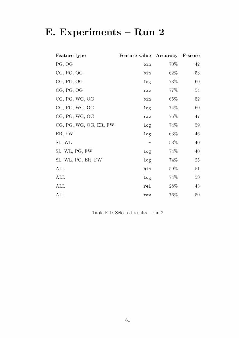
E. Experiments – Run 2

Feature type Feature value Accuracy F-score

PG, OG bin 70% 42

CG, PG, OG bin 62% 53

CG, PG, OG log 73% 60

CG, PG, OG raw 77% 54

CG, PG, WG, OG bin 65% 52

CG, PG, WG, OG log 74% 60

CG, PG, WG, OG raw 76% 47

CG, PG, WG, OG, ER, FW log 74% 59

ER, FW log 63% 46

SL, WL - 53% 40

SL, WL, PG, FW log 74% 40

SL, WL, PG, ER, FW log 74% 25

ALL bin 59% 51

ALL log 74% 59

ALL rel 28% 43

ALL raw 76% 50

Table E.1: Selected results – run 2

61

62

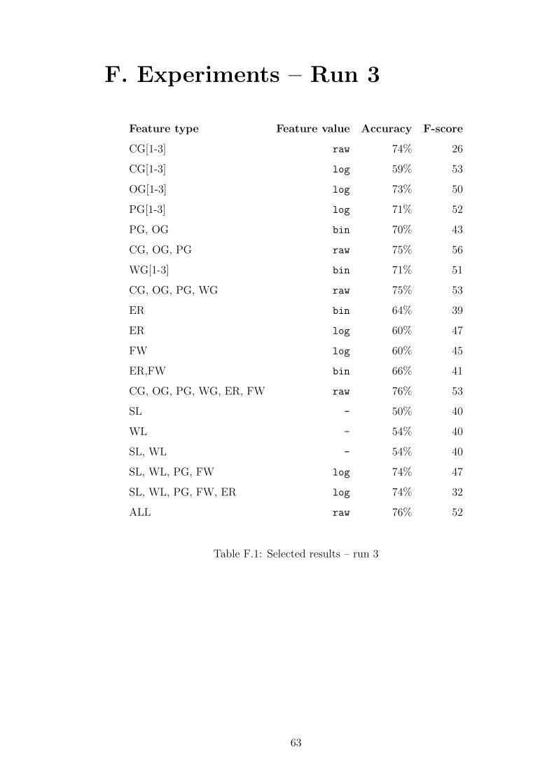
F. Experiments – Run 3

Feature type Feature value Accuracy F-score

CG[1-3] raw 74% 26

CG[1-3] log 59% 53

OG[1-3] log 73% 50

PG[1-3] log 71% 52

PG, OG bin 70% 43

CG, OG, PG raw 75% 56

WG[1-3] bin 71% 51

CG, OG, PG, WG raw 75% 53

ER bin 64% 39

ER log 60% 47

FW log 60% 45

ER,FW bin 66% 41

CG, OG, PG, WG, ER, FW raw 76% 53

SL - 50% 40

WL - 54% 40

SL, WL - 54% 40

SL, WL, PG, FW log 74% 47

SL, WL, PG, FW, ER log 74% 32

ALL raw 76% 52

Table F.1: Selected results – run 3

63

64

G. Features by Information Gain

– Selected plots

0 2000 4000 6000 8000 10000

0.00

00.

005

0.01

00.

015

0.02

00.

025

Number of features

Info

rmat

ion

Gai

n

Figure G.1: Character n-grams, log

0 5000 10000 15000 20000 25000

0.00

00.

002

0.00

40.

006

0.00

80.

010

0.01

20.

014

Number of features

Info

rmat

ion

Gai

n

Figure G.2: Word n-grams, log

0 1000 2000 3000 4000 5000 6000

0.00

00.

005

0.01

00.

015

0.02

00.

025

0.03

0

Info

rmat

ion

Gai

n

Figure G.3: POS n-grams, log

0 5000 10000 15000

0.00

00.

005

0.01

00.

015

Number of features

Info

rmat

ion

Gai

n

Figure G.4: OC-POS n-grams, log

65

66

H. Top features by Information

Gain – Examples

1

2

3

4

5

6

7

8

9

10

c h

h

s v

h o

r u s

l ı

ı b ı

r u

z

z a

lıbı

uz

rusku

sebou

ze

ruska

bych

mnoho

ruznych

take

Table H.1: Top 10 features according to Information Gain – CG3bin, WG1bin

67

1

2

3

4

5

6

7

8

9

10

Cap0

Quant1

Caron0

Quant0

SingCh

VoicedFin1

Caron1

Y1

Voiced

Y0

Table H.2: Top 10 features according to Information Gain – ERlog

1

2

3

4

5

6

7

8

9

10

P8 NN

Vc Vf

Ca AA

Vp Vc

RR P5

PD Db

TT RR

RR AA

AA NN

P8 AA

VC VF

VB ?

VP VC

JAK SE

TVUJ NN

NA AA

AA NN

NN ,

MNOHO AA

SVOU NN

Table H.3: Top 10 features according to Information Gain – PG2bin, OG2bin

68

69

70

Attachments

The whole project, together with data and documentation is available at

https://bitbucket.org/jhana/students-lida.

71

72