natural algorithms and influence systemschazelle/pubs/cacm12-natalg.pdf · and influence systems by...

december 2012 | vol. 55 | no. 12 | communications of the acm 101

Doi:10.1145/2380656.2380679

Natural Algorithms and Influence SystemsBy Bernard Chazelle

abstractAlgorithms offer a rich, expressive language for modelers of biological and social systems. They lay the grounds for numerical simulations and, crucially, provide a powerful framework for their analysis. The new area of natural algo-rithms may reprise in the life sciences the role differential equations have long played in the physical sciences. For this to happen, however, an “algorithmic calculus” is needed. We discuss what this program entails in the context of influ-ence systems, a broad family of multiagent models arising in social dynamics.

1. intRoDuctionThe gradual elevation of “computational thinking” within the sciences is enough to warm the heart of any computer sci-entist. Yet the long-awaited dawning of a new age may need to wait a little longer if we cannot move beyond the world of simulation and build a theory of natural algorithms with real analytical heft. By “natural algorithms,” I mean the myriad of algorithmic processes evolved by nature over millions of years. Just as differential equations have given us the tools to explain much of the physical world, so will natural algo-rithms help us model the living world and make sense of it. At least this is the hope and, for now, I believe, one of the most pressing challenges facing computer science.

1.1. science or engineering?To draw a fine line between science and engineering is a fool’s errand. Unrepentant promiscuity makes a clean separation neither wise nor easy. Yet a few differences bear mentioning. If science is the study of the nature we have, then engineering is the study of the nature we want: the scientist will ask how the valley was formed; the engineer will ask how to cross it. Science is driven by curiosity and engineering by need: one is the stuff of discovery, the other of invention. The path of science therefore seems more narrow. We want our physical laws to be right and our mousetraps to be useful. But there are more ways to be useful than to be right. Engineering can “negotiate” with nature in ways science cannot. This freedom comes at a price, however. Any mousetrap is at the mercy of a better one. PageRank one day will go; the Second Law of ther-modynamics never will. And so algorithms, like mousetraps, are human-designed tools: they are engineering artifacts.

Or are they? Perhaps search engines do not grow on trees, but leaves do, and a sophisticated algorithmic formalism, L-systems, is there to tell us how20. It is so spectacularly accu-rate, in fact, that the untrained eye will struggle to pick out computer-generated trees from the real thing. The algorith-mic modeling of bird flocking has been no less successful.

Some will grouch that evolution did not select the human eye for its capacity to spot fake trees and catch avian impostors. Ask a bird to assess your computer-animated flock, they will snicker, and watch it cackle with derision. Perhaps, but the oohs and ahhs from fans of CGI films everywhere suggest that these models are on to something. These are hardly isolated cases. Natural algorithms are quickly becoming the language of choice to model biological and social processes. And so algo-rithms, broadly construed, are both science and engineering.

1.2. it is all about languageThe triumph of 20th-century physics has been, by and large, the triumph of mathematics. A few equations scattered on a single page of paper explain most of what goes on in the physical world. This miracle speaks of the organizing princi-ples of the universe: symmetry, invariance, and regularity—precisely the stuff on which mathematics feasts. Alas, not all of science is this tidy. Biology = physics + history; but history is the great, unforgiving symmetry breaker. Instead of iden-tical particles subject to the same forces, the life sciences feature autonomous agents, each one with its own idea of what laws to obey. It is a long way, scientifically speaking, from planets orbiting the sun in orderly fashion to unruly slime molds farming bacterial crops. Gone are the symme-try, invariance, and clockwork regularity of astronomy: what we have is, well, sludge. But the sludge follows a logic that has its own language, the language of natural algorithms.

The point of departure with classical mathematics is indeed linguistic. While differential equations are the native idiom of electromagnetism, no one believes that cancer has its own “Maxwell’s equations.” Yet it may well have its own natural algorithm. The chain of causal links, some deter-ministic, others stochastic, cannot be expressed solely in the language of differential equations. It is not just the diversity of factors at play (genetic, infectious, environmental, etc.); nor is it only their heterogeneous modes of interaction. It is also the need for a narrative of collective behavior that can be expressed at different levels of abstraction: first-princi-ples; phenomenological; systems-level; and so on. The issue is not size alone: the 3-body problem may be intractable but, through the magic of universality, intricate phase transitions among 1030 particles can be predicted with high accuracy. The promise of agent-based natural algorithms is to deliver tractable abstractions for descriptively complex systems.

This paper is based on “Natural Algorithms,” which was published in the Proceedings of the 20th Annual ACM-SIAM Symposium on Discrete Algorithms, 2009, and subsequent work.

102 communications of the acm | december 2012 | vol. 55 | no. 12

research highlights

maximal independent sets in fly brain development1, and so on. Consensus, synchronization, and fault tolerance are concepts central to both biology and distributed comput-ing15, 17. The trade of ideas promises to be flowing both ways. This article focuses on the outbound direction: how algo-rithmic ideas can enrich our understanding of nature.

2. infLuence sYstemsA bad, fanciful script will make a good stage-setter. One fate-ful morning, you stumble out of bed and into your kitchen only to discover, crawling on the floor, a swarm of insects milling around. Soon your dismay turns to curiosity, as you watch the critters engage in a peculiar choreography. Each insect seems to be choosing a set of neighbors (living or inert) and move either toward or away from them. From what you can tell, the ants pick the five closest termites; the termites select the nearest soil pellets; the ladybugs pick the two ants closest to the powdered sugar that is not in the vicinity of any termite; and so on. Each insect seems equipped with its own selection procedure to decide how to pick neighbors based on their species and the local environment. Once the selec-tion is made, each agent invokes a second procedure, this time to move to a location determined entirely by the iden-tities and positions of its neighbors. To model this type of multiagent dynamics, we have introduced influence systems6: the model is new, but only new to the extent that it unifies a wide variety of well-studied domain-dependent systems. Think of influence systems as a brand of networks that per-petually rewire themselves endogenously.

2.1. Definition and examplesAn influence system, is specified by two functions f and G: it is a discrete-time dynamical system,b x f (x) in (Rd)n, where n is the number of agents, d is the dimension of the ambient space (d = 2 in the example above), and each “coordinate” xi of the state x = (x1, . . . , xn) ∈ (Rd)n is a d-tuple encoding the location of agent i in Rd. With any state x comes a directed “communication” graph, G (x), with one node per agent. Each coordinate function fi of the map f = ( f1, . . . , fn) takes as input the neighbors of agent i in G (x), together with their locations, and outputs the new location fi(x) of agent i in Rd. The (action) function f and (communication) function G are evaluated by deterministic or randomized algorithms. An influence sys-tem is called diffusive if f keeps each agent within the convex hull of its neighbors. Diffusive systems never escape to infin-ity and always make consensus (x1 = . . . = xn) a fixed point. The system is said to be bidirectional if the communication graph always remains undirected.

While f and G can be arbitrary functions, the philosophy behind influence systems is to keep f simple so that emer-gent phenomena can be attributed not so much to the power of individual agents, but to the flow of information across the communication network G (x). By distinguishing G from f, the model also separates the syntactic (who talks to whom?)

1.3. What is complexity?Such is the appeal of the word “complexity” that it comes in at least four distinct flavors.

• Semantic: What is hard to understand. For 99.99% of mankind, complex means complicated.

• Epistemological: What is hard to predict. An indepen-dent notion altogether: complex chaotic systems can be simple to understand while complicated mecha-nisms can be easy to predict.

• Instrumental: What is hard to compute, the province of theoretical computer science.

• Linguistic: What is hard to describe. Physics has low descriptive complexity—that is part of its magic.a By contrast, merely specifying a natural algorithm may require an arbitrarily large number of variables to model the diversity present in the system. To capture this type of complexity is a distinctive feature of natural algorithms.

1.4. beyond simulationDecades of work in programming languages have produced an advanced theory of abstraction. Ongoing work on reactive systems is attempting to transfer some of this technology to biology9. Building on years of progress in automata theory, temporal logic, and process algebra, the goal has been to build a modeling framework for biological systems that integrate the concepts of concurrency, interaction, refine-ment, encapsulation, modularity, stochasticity, causality, and so on. With the right specifications in place, the hope is that established programming language tools, such as type theory, model checking, abstract interpretation, and the pi-calculus can aid in verifying temporal properties of biosys-tems. The idea is to reach beyond numerical simulation to analyze the structure and interactions of biological systems.

Such an approach, however, can only be as powerful as the theory of natural algorithms behind it. To illustrate this point, consider classifying all possible sequences x, Px, P2x, P3x, and so on, where x is a vector and P is a fixed stochas-tic matrix. Simulation, machine learning, and verification techniques can help, but no genuine understanding of the process can be achieved without Perron–Frobenius theory. Likewise, natural algorithms need not only computers but also a theory. The novelty of the theory will be its reliance on algorithmic proofs—more on this below.

1.5. algorithms from natureIf living processes are powered by the “software” of nature, then natural selection is the ultimate code optimizer. With time and numbers on their side—billions of years and 1030 living specimens—bacteria have had ample opportunity to perfect their natural algorithm. No wonder computer sci-entists are turning to biology for algorithmic insight: neu-ral nets and DNA computing, of course, but also ant colony optimization3, shortest path algorithms in slime molds2;

a Descriptive complexity is an established subfield of theoretical computer science and logic. Our usage is a little different, but not different enough to warrant a change of terminology.

b A dynamical system generates an orbit by starting at a point x and iterating the function f to produce f (x), f 2(x), and so on. The goal is to understand the geometry of these orbits. We write the phase space Rdn as (Rd)n to emphasize that the action is on the n agents embedded in d-space.


from the semantic (who does what?). It is no surprise then to see recursive graph algorithms play a central role and pro-vide a dynamic version of renormalization, a technique used in quantum mechanics and statistical physics.

• Bounded-confidence systems: In this popular model of social dynamics10, d = 1 and xi is a real number denoting the “opinion” of agent i. That agent is linked to j if and only if |xi − xj| ≤ 1. The action function f instructs each agent to move to the mass center of their neighbors. This is the prototypical example of a bidirectional dif-fusive influence system.

• Sync: An instance of Kuramoto synchronization, this diffusive influence system links each of n fireflies to the other fireflies whose flashes it can spot. Every critter has its own flashing oscillator, which becomes coupled with those of its neighbors. The function f specifies how the fireflies adjust their flashings in reaction to the graph-induced couplings3, 23. The model has been applied to Huygens’s pendulum clocks as well as to circadian neu-rons, chirping crickets, microwave oscillators, yeast cell suspensions, and pacemaker cells in the heart25.

• Swarming: The agents may be fish or birds, with states encoding positions and velocities (for rigid 3D animal models, d = 9). The communication graph links every agent to some of its nearest neighbors. The function f instructs each agent to align its velocity with those of its neighbors, to move toward their center of gravity, and to fly away from its perilously close neighbors21, 24.

• Chemotaxis: Some organisms can sense food gradients and direct their motion accordingly. In the case of bac-terial chemotaxis, the stimuli are so weak that the organisms are reduced to performing a random walk with a drift toward higher food concentrations. Influence systems can model these processes with the use of both motile and inert agents.c Chemotaxis is usually treated as an asocial process (single agents interacting only with the environment). It has been observed, however, that schooling behavior can facili-tate gradient climbing for fish, a case where living in groups enhances foraging ability19.

Other examples of influence systems include the Ising model, neural nets, Bayesian social learning, protein–protein interaction networks, population dynamics, and so on.

2.2. how expressive are influence systems?If agent i is viewed as a computing device, then the d-tuple xi is its memory. The system is Markovian in that all facts about the past with bearing on the future are encoded in x. The communication graph allows the function f to be local if so desired. The procedure G itself might be local even when appearance suggests otherwise: for example, to identify

your nearest neighbor in a crowd entails only local com-putation, although, mathematically, the function requires knowledge about everyone. The ability to encode different action/communication rules for each agent is what drives up the descriptive complexity of the system. In return, one can produce great behavioral richness even in the presence of severe computational restrictions.

(i) Learning, competition, hierarchy: Agents can imple-ment game-theoretic strategies in competitive envi-ronments (e.g., pursuit-evasion games) and learn to cooperate in groups (e.g., quorum sensing). They can self-improve, elect leaders, and stratify into domi-nance hierarchies.

(ii) Coarse-graining: Flocks are clusters of birds that maintain a certain amount of communicative cohe-sion over a period of time. We can view them as “super-agents” and seek the rules governing interac-tion among them. Iterating in this fashion can set the stage for dynamic renormalization in a time- changing analog of the renormalization group of sta-tistical mechanics (see Section 6).

(iii) Asynchrony and uncertainty: In the presence of delayed or asynchronous communication, agents can use their memory to implement a clock for the purpose of time stamping. Influence systems can also model uncertainty by limiting agents’ access to approximations of their neighbors’ states.

A few words about our agent-based approach. Consider the diffusion of pollen particles suspended in water. A Eulerian approach to this process seeks a differential equation for the concentration c (x, t) of particles at any point x and time t. There are no agents, just density func-tions evolving over time18. An alternative approach, called Lagrangian, would track the movement of all the individual particles and water molecules by appealing to Newton’s laws. Given the sheer number of agents, this line of attack crashes against a wall of intractability. One way around it is to pick a single imaginary self-propelled agent and have it jiggle about randomly in a Brownian motion. This agent models a typical pollen particle—typical in the “ergodic” sense that its time evolution mimics the space distribution of countless particles caught on film in a snapshot. Scaling plays a key role: our pollen particles indeed can be observed only on a timescale far larger than the molecular bumps causing the jiggling. Luckily, Brownian motion is scale-free, meaning that it can be observed at any scale. As we shall see in Section 6, the ability to express a dynamical process at dif-ferent scales is an important feature of influence systems.

The strength of the Eulerian approach is its privileged access to an advanced theory of calculus. Its weakness lies in two commitments: global behavior is implied by infini-tesimal changes; and every point is subject to identical laws. While largely true in physics, these assumptions break down in the living world, where diversity, heterogeneity, and autonomy prevail. Alas, the Lagrangian answer, agent-based modeling, itself suffers from a serious handicap: the lack of a theory of natural algorithms.

c Some living systems (e.g., ants and termites) exchange information by stig-mergy: instead of communicating directly with signals, they leave traces such as pheromones in the environment, which others then use as cues to coor-dinate their collective work. Although lacking autonomy, inert components can still be modeled as agents in an influence system.


research highlights

2.3. What could go wrong?There are two arguments against the feasibility of a domain-independent theory of natural algorithms. One is an intrin-sic lack of structure. But the same can be said of graphs, a subject whose ties to algebra, geometry, and topology have met with resounding success, including the emergence of universality. A more serious objection is that, before we can analyze a natural algorithm, we must be able to specify it. The bottom-up, reductionist approach, which consists of specifying the functionality and communicability of each agent by hand (as is commonly done in swarming models), might not always work. Sometimes, only a top-down, phe-nomenological approach will get us started on the right track. We have seen this before: the laws of thermodynamics were not derived as abstractions of Newton’s laws—though that is what they are—but as rules governing observable macrostates (P, V, T, and all that). Likewise, a good flock-ing model might want to toss aside anthropomorphic rules (“stay aligned,” “don’t stray,” etc.) and choose optimized statistical rules inferred experimentally. The specs of the natural algorithm would then be derived algorithmically. This is why we have placed virtually no restriction on the communication function G in our present analysis of diffu-sive influence systems.

2.4. outlineWe open the discussion in Section 3 with the total s-energy, a key analytical device used throughout. We turn to bird flock-ing in Section 4, which constitutes the archetypical nondif-fusive influence system. We take on the diffusive case in Section 5, with the notion of algorithmic calculus discussed in Section 6.d General diffusive influence systems are Turing-complete, yet the mildest perturbation creates periodic behavior. This is disconcerting. Influence systems model how people change opinions over time as a result of human interaction and knowledge acquisition. Instead of ascend-ing their way toward enlightenment, however, people are doomed to recycle the same opinions in perpetuity—there is a deep philosophical insight there, somewhere.

3. the -eneRGYThis section builds the tools needed for the bidirectional case and can be read separately from the rest. Let (Pt)t≥ 0 be an infinite sequence of n-by-n stochastic matrices; stochas-tic means that the entries are nonnegative and the rows sum up to 1. Leaving aside influence systems for a moment, we make no assumption about the sequence, not even that it is produced endogenously. We ask a simple question about matrix sequences: under what conditions does P<t : = Pt –1 . . . P0 converge as t → ∞? Certainly not if

The problem here is lack of self-confidence: the two agents in the system do not trust themselves and follow their

neighbors blindly. So let us assume that the diagonal entries of Pt are positive. Alas, this still does not do the trick: the matrices

grant the agents self-confidence, yet composing them in alternation exchanges the vectors (0, 1, 1/4) and (0, 1, 3/4) endlessly. The oscillation is caused by the lack of bidi-rectionality: for example, the recurring link from agent 3 to agent 1 is never reciprocated. The fix is to require the graphs to be undirected or, equivalently, the matrices to be type-symmetric,e which instills mutual confidence among the agents. With both self-confidence and bidirec-tionality in place, the sequence P<t always converges12, 14, 16. (Interestingly, this is not true of forward products P0 . . . Pt in general.) With nothing keeping (Pt )t ≥ 0 from “stalling” by featuring arbitrarily long repeats of the identity matrix, bounding the convergence rate is obviously impossible. Yet an analytical device, the total s-energy5, allows us to do just that for bidirectional diffusive influence systems. The trick is to show that they cannot stall too long without dying off.

3.1. PreliminariesFix a small r > 0 and let (Pt )t ≥ 0 be a sequence of stochastic matrices such that r ≤ (Pt )ii ≤ 1 − r and (Pt )ij > 0 ⇒ (Pt)ji > 0. Let Gt be the (undirected) graph whose edges are the positive entries in Pt. With x(t + 1) = Pt x(t) and x(0) = x ∈ [0, 1]n, the total s-energy is defined as

(1)

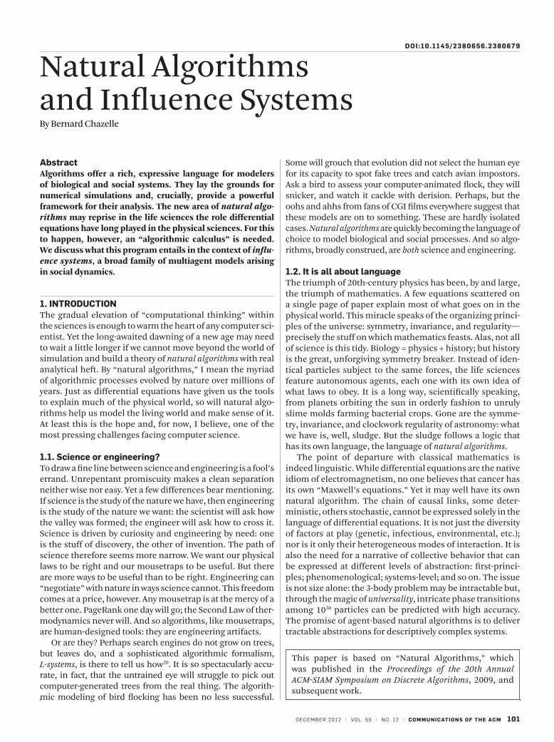
We use the s-energy in much the same way one uses Chernoff’s inequalities to bound the tails of product distri-butions. Being a generalized Dirichlet series, the s-energy can be inverted and constitutes a lossless encoding of the edge lengths. Why this unusual choice? Because, as with the most famous Dirichlet series of all, the Riemann zeta function Σn–s, the system’s underlying structure is multi-plicative: indeed, just as n is a product of primes, xi(t) − xj(t) is a product of the form vT Pt−1 . . . P0 x. Let En(s) denote the maximum value of E(s) over all x ∈ [0, 1] n. One should expect the function En(s) to encode all sorts of symmetries. This is visible in the case n = 2 by observing that it can be continued meromorphically in the whole complex plane (Figure 1).

The sequence formed by (Pt )t ≥ 0 is called reversible if Gt is connected and there is a probability distribution (p1, . . . , pn) such that pi(Pt )ij = pj(Pt )ji for any t; see detailed definition in Chazelle5. This gives us a way to weight the agents so that their mass center never moves. The notion general-izes the concept of reversible Markov chains, with which it shares some of the benefits, including faster conver-gence to equilibrium.

d Unless noted otherwise, the results discussed are from Chazelle5 for Section 3; Chazelle4 for Section 4; Chazelle6 for sections 5 and 6.

e The zero-entries of a type-symmetric matrix and its transpose occur at the same locations.


3.2. boundsThe s-energy measures the total length of all the edges for s = 1 and counts their number for s = 0; the latter is usually infi-nite, so it is sensible to ask how big En(s) can be for 0 < s ≤ 1. On the lower bound front, we have En(1) = W(1/r) n/2 and En(s) = s1−n(1/ r)W(n), for any n large enough, s ≤ s0, and any fixed positive s0 < 1. Of course, the s-energy is useful mostly for its upper bounds5:

(2)

For reversible sequences and any 0 < s ≤ 1.

(3)

where . This is essentially optimal. Fix an arbitrarily small e > 0. A step t is called trivial if |xi(t) − xj(t)| < e for each (i, j) ∈ Gt. The maximum number Ce of nontrivial steps is bounded by e−s En(s); hence,

(4)

which is optimal if e is not too small. Convergence in the reversible case is polynomial: if e < r/n, then x(t) − pTx2 ≤ e, for t = O(r−1 n2|log e|). This bound is optimal. In particular, we can specialize it to the case of random walks in undi-rected graphs and retrieve the usual mixing times.

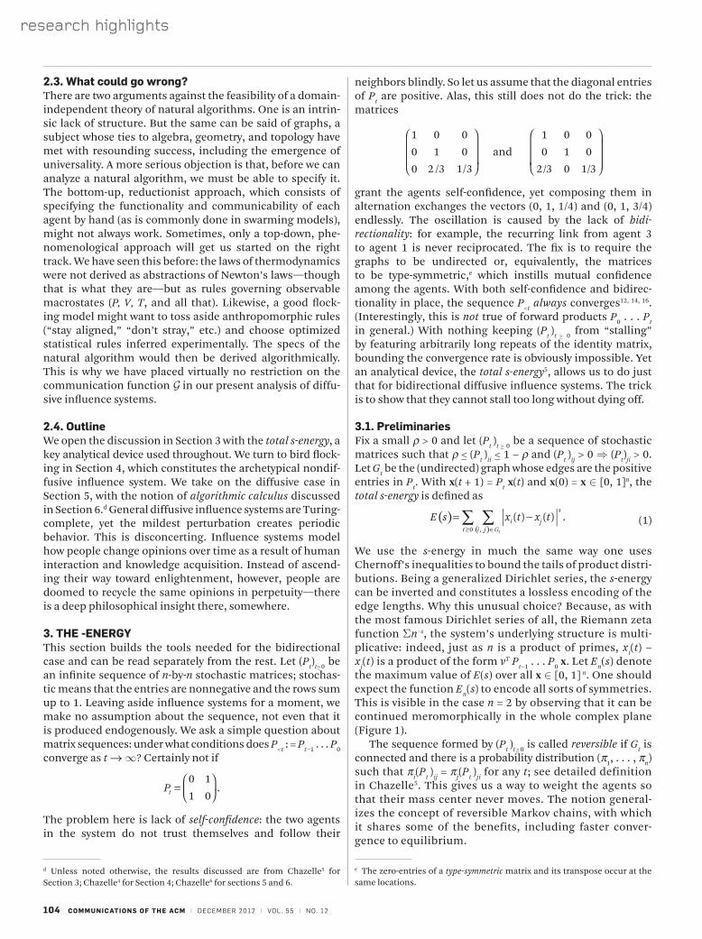
We briefly mention two examples of diffusive influence systems for which the s-energy readily yields bounds on the convergence time5. HK systems track opinion polariza-tion in a population10: in the bounded-confidence version (mentioned earlier), the agents consist of n points in Rd. At each step, each agent moves to the mass center of the agents within distance 1 (Figure 2).

Truth-seeking systems assume a “cognitive division of labor”11. We fix one agent, the truth, and keep the n − 1 oth-ers mobile. A “truth seeker” is a mobile agent that is joined to the truth in every Gt. All the other mobile agents are “igno-rant,” meaning that they never join to the truth through an edge, although they might indirectly communicate with it

along a path. Any two mobile agents are joined in Gt whenever their distance is less than 1.

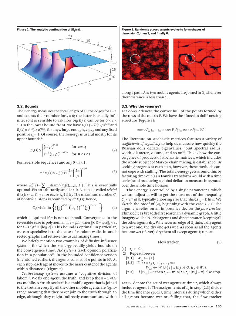
3.3. Why the -energy?Let convP denote the convex hull of the points formed by the rows of the matrix P. We have the “Russian doll” nesting structure (Figure 3):

The literature on stochastic matrices features a variety of coefficients of ergodicity to help us measure how quickly the Russian dolls deflate: eigenvalues, joint spectral radius, width, diameter, volume, and so on22. This is how the con-vergence of products of stochastic matrices, which includes the whole subject of Markov chain mixing, is established. By seeking progress at each step, however, these methods can-not cope with stalling. The total s-energy gets around this by factoring time out (as a Fourier transform would with a time series) and producing a global deflation measure integrated over the whole time horizon.

The s-energy is controlled by a single parameter s, which we can adjust at will to get the most out of the inequality Ce ≤ e−s E(s), typically choosing s so that (dE/ds)|s = E ln e. We sketch the proof of (2), beginning with the case s < 1. The argument relies on an importance device: the flow tracker. Think of it as breadth-first search in a dynamic graph. A little imagery will help. Pick agent 1 and dip it in water, keeping all the other agents dry. Whenever an edge of Gt links a dry agent to a wet one, the dry one gets wet. As soon as all the agents become wet (if ever), dry them all except agent 1; repeat.

Flow tracker (5)

[1] t0 ← 0.[2] Repeat forever:

[2.1] Wt0 ← {1}.

[2.2] For t = t0, t0 + 1, . . . , ∞:Wt+1 ← Wt ∪ { i | ∃ (i, j) ∈ Gt & j ∈ Wt }.

[2.3] If |W∞| = n then t0 ← min{t > t0 : |Wt| = n} else stop.

Let Wt denote the set of wet agents at time t, which always includes agent 1. The assignments of t0 in step [2.3] divide the timeline into epochs, time intervals during which either all agents become wet or, failing that, the flow tracker

2015

105

0

1.5

1.0

0.5

0.010

5

0

figure 1. the analytic continuation of |e2(s)|. figure 2. Randomly placed agents evolve to form shapes of dimension 2, then 1, and finally 0.


research highlights

comes to a halt (breaking out of the repeat loop at “stop”). Take the first epoch: it is itself divided into subintervals by the coupling times t1 < . . . < tl at which the set of wet agents grows: Wtk Wtk+1. If Wt denotes the length of the small-est interval enclosing Wt, it can be shown by induction that Wtk+1 ≤ 1 –ρk. It then follows that E1(s) = 0 and, for n ≥ 2,

En (s) ≤ 2nEn – 1 (s) + (1–ρn)s En(s) + n3,

which implies (2) for s < 1.The case s = 1 features a fundamental concept in the study

of natural algorithms, that of an algorithmic proof. Think of the agents as car drivers: the 1-energy can then be shown to mea-sure the total mileage. Fill the gas tank of each car with an initial amount determined by some formula (whose details are immaterial for our purposes). Since we do not know ahead of time how much gas any given car will need, we set up a gas trading mechanism: a refueling tanker hovers over the cars, ready to provide (or take) gas to (or from) any car that needs it. The needs come in two ways: first, a car needs gas to move; second, the trading mechanism specifies how much gas any car must have at any time, so any excess supply must be handed over to the refueling tanker. Any car in need of gas (for driving or simply complying with the rules) is free to help itself from the fuel tanker. The trick is to show that the system can run forever without the fuel tanker ever run-ning out of gas and being unable to meet the drivers’ needs.

Dynamicists might think of this as a kind of distrib-uted Lyapunov function. This would be missing the point. Algorithmic proofs of the type found in the amortized analysis of algorithms—often expressed, as above, via the trading rules of a virtual economy—are meant to cope with the sort of descriptive complexity typically absent from low-dimensional dynamics. The benefits come from the richer analytical language of algorithmic proofs: indeed, it is all about language!

4. biRD fLocKinGWe briefly discuss a classic instance of a nondiffusive influence system, bird flocking, and report the results from Chazelle4. The alignment model we use8, 13, 24 is a

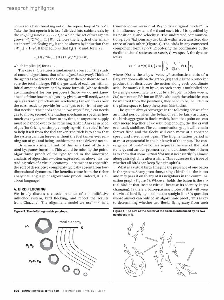
trimmed-down version of Reynolds’s original model21. In this influence system, d = 6 and each bird i is specified by its position zi and velocity vi. The undirected communica-tion graph G (x) joins any two birds within a certain fixed dis-tance of each other (Figure 4). The birds in any connected component form a flock. Reordering the coordinates of the 6n-dimensional state vector x as (z, v), we specify the dynam-ics as

where Q(x) is the n-by-n “velocity” stochastic matrix of a (lazy) random walk on the graph G (x) and ⊗ is the Kronecker product that distributes the action along each coordinate axis. The matrix P is 2n-by-2n, so each entry is multiplied not by a single coordinate in x but by a 3-tuple; in other words, P(x) acts not on R2n but on (R3)2n. Although the velocities can be inferred from the positions, they need to be included in the phase space to keep the system Markovian.

The system always converges in the following sense: after an initial period when the behavior can be fairly arbitrary, the birds aggregate in flocks which, from that point on, can only merge together. If we wait long enough, the flocks will eventually stabilize. The communication graph will remain forever fixed and the flocks will each move at a constant speed and never meet again. The fragmentation period is at most exponential in the bit length of the input. The con-vergence of birds’ velocities requires the use of the total s-energy and various geometric considerations. One of them is to show that some virtual bird must necessarily fly almost along a straight line after a while. This addresses the issue of whether all birds can keep flying in spirals.

What is a virtual bird? Imagine the presence of one baton in the system. At any given time, a single bird holds the baton and may pass it on to any of its neighbors in the communi-cation graph (Figure 5). Whoever holds the baton is the vir-tual bird at that instant (virtual because its identity keeps changing). Is there a baton-passing protocol that will keep the virtual bird flying in (almost) a straight line? (A question whose answer can only be an algorithmic proof.) This is key to determining whether two flocks flying away from each

total s-energy

SP0

P1P0

P2P1P0

figure 3. the deflating matrix polytope. figure 4. the bird at the center of the circle is influenced by its two neighbors in it.


other can be brought together by other flocks. The design of a protocol involves the geometric analysis of the flight net (Figure 6), which is the unfolding of all neighboring relations in four-dimensional spacetime. This is a tree-like geometric object in R4 with local convexity properties, which encodes the exponentially large number of influences among birds. The position of each bird can be expressed by a path integral in that space. Examining these integrals (actually sums) and the geometry that produces them allows us to answer the question above4.

While flocks cease to fragment reasonably rapidly (thus ensuring quick physical convergence), it might take very long for them to stop merging. How long? A tower-of-twos of height logarithmic in the number of birds. Surprisingly, this result is tight! To prove that, we regard the set of birds as forming a computer and we ask a “busy-beaver” type of question: What is the smallest nonzero angle between any two stationary veloci-ties? The term “stationary” refers to the fact that each flock is a coupled oscillator with constant stationary velocity (the low-est mode of its spectrum). These velocity vectors form angles between them. How small can they get short of 0? (Zero angles correspond to flocks flying in parallel.) To answer this question requires looking at the flocks of birds as a circuit whose gates, enacting flock merges, produce a redistribution of the energy among the modes called a spectral shift. It is remarkable that the busy-beaver function of this exotic computing device can

be pinned down almost exactly: the logarithmic height of the tower-of-twos is known up to a factor of 4.

5. DiffusiVe infLuence sYstemsWe set f (x) = (P(x) ⊗ Id) x ∈ (Rd)n, where P(x) is a stochas-tic matrix whose positive entries correspond to the edges of G (x) and are rationals assumed larger than some arbi-trarily small r > 0. We grant the agents a measure of self-confidence by adding a self-loop to each node of G (x). Agent i computes the i-th row of P(x) by means of its own algebraic decision tree; that is, on the basis of the signs of a finite number of dn-variate polynomials evaluated at the coordinates of x. This high level of generality allows G (x) to be specified by any first-order sentence over the reals.f Note how the descriptive complexity resides in the communica-tion algorithm G, which can be arbitrarily expressive: the action f is confined to diffusion (with different weights for each agent if so desired).

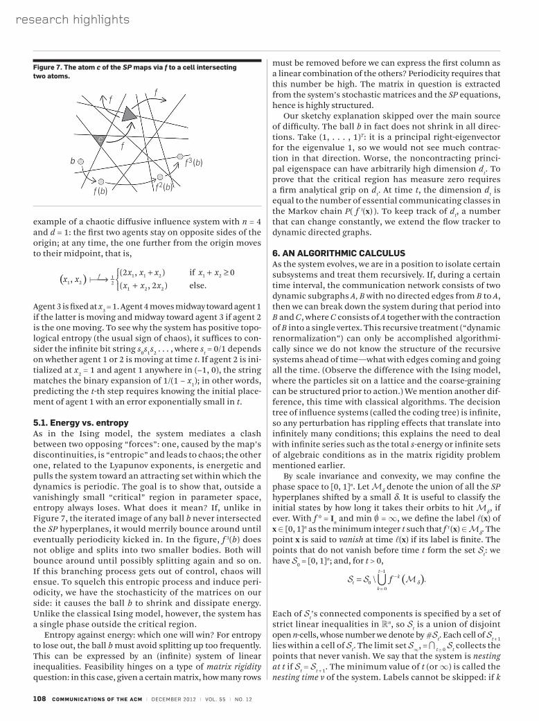
By taking tensor powers (no details needed here), we can linearize the system and reduce the dimension to d = 1, so f (x) = P(x)x, where P(x) = Pc, for any x ∈ c, and c is an atom (open n-cell) of an arrangement of hyperplanes in Rn, called the switching partition SP (Figure 7). We assume self- confidence but not mutual confidence, that is, positive diagonal entries but not necessarily bidirectionality.

In spite of having no positive Lyapunov exponents, dif-fusive systems can be chaotic and even Turing-complete. Perturbations wipe out their computational power, how-ever, by making them attracted to periodic orbits. Such sys-tems, in other words, are clocks in disguise.g This dichotomy requires a subtle bifurcation analysis, which we sketch in the next section.

Theorem 1:6 Given any initial state, the orbit of a diffusive influence system is attracted exponentially fast to a limit cycle almost surely under an arbitrarily small perturbation. The period and preperiod are bounded by a polynomial in the reciprocal of the failure probability. In the bidirectional case, the system is attracted to a fixed point in time nO(n)|log e|, where n is the number of agents and e is the distance to the fixed point.

The number of limit cycles is infinite, but if we mea-sure distinctness the right way (i.e., by factoring out folia-tions), there are actually only a finite number of them.h The critical region of parameter space is where chaos, strange attractors, and Turing completeness reside. It is still very mysterious.i This does not mean that it is difficult to iden-tify at least some of the critical points. Here is a simple

figure 5. the virtual bird can hold on to the baton or pass it to any neighbor.

figure 6. the flight net and path integrals in R4.

f This is the language of geometry and algebra over the reals with statements specified by any number of quantifiers and polynomial (in)equalities. It was shown to be decidable by Tarski and amenable to quantifier elimination and algebraic cell decomposition by Collins7.g To perturb the system means randomly perturbing the switching partition and making exceptions for infinitesimal and indefinitely disappearing edges. The conditions are easy to enforce and, in one form or another, required. Note that we do not perturb the matrices or the initial states.h A limit cycle is an attracting periodic orbit, for example, {−1, 1} where x(t) = (−1)t + 2−t x(t−1) and x(0) ∈ R.i I only know that the critical region has measure zero and looks like a Cantor set.


research highlights

example of a chaotic diffusive influence system with n = 4 and d = 1: the first two agents stay on opposite sides of the origin; at any time, the one further from the origin moves to their midpoint, that is,

Agent 3 is fixed at x3 = 1. Agent 4 moves midway toward agent 1 if the latter is moving and midway toward agent 3 if agent 2 is the one moving. To see why the system has positive topo-logical entropy (the usual sign of chaos), it suffices to con-sider the infinite bit string s0s1s2 . . . , where st = 0/1 depends on whether agent 1 or 2 is moving at time t. If agent 2 is ini-tialized at x2 = 1 and agent 1 anywhere in (−1, 0), the string matches the binary expansion of 1/(1 − x1); in other words, predicting the t-th step requires knowing the initial place-ment of agent 1 with an error exponentially small in t.

5.1. energy vs. entropyAs in the Ising model, the system mediates a clash between two opposing “forces”: one, caused by the map’s discontinuities, is “entropic” and leads to chaos; the other one, related to the Lyapunov exponents, is energetic and pulls the system toward an attracting set within which the dynamics is periodic. The goal is to show that, outside a vanishingly small “critical” region in parameter space, entropy always loses. What does it mean? If, unlike in Figure 7, the iterated image of any ball b never intersected the SP hyperplanes, it would merrily bounce around until eventually periodicity kicked in. In the figure, f 3(b) does not oblige and splits into two smaller bodies. Both will bounce around until possibly splitting again and so on. If this branching process gets out of control, chaos will ensue. To squelch this entropic process and induce peri-odicity, we have the stochasticity of the matrices on our side: it causes the ball b to shrink and dissipate energy. Unlike the classical Ising model, however, the system has a single phase outside the critical region.

Entropy against energy: which one will win? For entropy to lose out, the ball b must avoid splitting up too frequently. This can be expressed by an (infinite) system of linear inequalities. Feasibility hinges on a type of matrix rigidity question: in this case, given a certain matrix, how many rows

must be removed before we can express the first column as a linear combination of the others? Periodicity requires that this number be high. The matrix in question is extracted from the system’s stochastic matrices and the SP equations, hence is highly structured.

Our sketchy explanation skipped over the main source of difficulty. The ball b in fact does not shrink in all direc-tions. Take (1, . . . , 1)T: it is a principal right-eigenvector for the eigenvalue 1, so we would not see much contrac-tion in that direction. Worse, the noncontracting princi-pal eigenspace can have arbitrarily high dimension dt. To prove that the critical region has measure zero requires a firm analytical grip on dt. At time t, the dimension dt is equal to the number of essential communicating classes in the Markov chain P( f t(x) ). To keep track of dt, a number that can change constantly, we extend the flow tracker to dynamic directed graphs.

6. an aLGoRithmic caLcuLusAs the system evolves, we are in a position to isolate certain subsystems and treat them recursively. If, during a certain time interval, the communication network consists of two dynamic subgraphs A, B with no directed edges from B to A, then we can break down the system during that period into B and C, where C consists of A together with the contraction of B into a single vertex. This recursive treatment (“dynamic renormalization”) can only be accomplished algorithmi-cally since we do not know the structure of the recursive systems ahead of time—what with edges coming and going all the time. (Observe the difference with the Ising model, where the particles sit on a lattice and the coarse-graining can be structured prior to action.) We mention another dif-ference, this time with classical algorithms. The decision tree of influence systems (called the coding tree) is infinite, so any perturbation has rippling effects that translate into infinitely many conditions; this explains the need to deal with infinite series such as the total s-energy or infinite sets of algebraic conditions as in the matrix rigidity problem mentioned earlier.

By scale invariance and convexity, we may confine the phase space to [0, 1]n. Let Md denote the union of all the SP hyperplanes shifted by a small d. It is useful to classify the initial states by how long it takes their orbits to hit Md , if ever. With f 0 = in and min 0/ = ∞, we define the label l(x) of x ∈ [0, 1]n as the minimum integer t such that f t (x) ∈ Md. The point x is said to vanish at time l(x) if its label is finite. The points that do not vanish before time t form the set St: we have S0 = [0, 1]n; and, for t > 0,

Each of St’s connected components is specified by a set of strict linear inequalities in Rn, so St is a union of disjoint open n-cells, whose number we denote by #St. Each cell of St + 1 lies within a cell of St. The limit set S∞, = ∩ t ≥ 0 St collects the points that never vanish. We say that the system is nesting at t if St = St + 1. The minimum value of t (or ∞) is called the nesting time v of the system. Labels cannot be skipped: if k

f

ff

f3(b)

c

f2(b)f(b)

b

figure 7. the atom c of the SP maps via f to a cell intersecting two atoms.


is a label, then so is k − 1. It follows that the nesting time v is the minimum t such that, for each cell c of St, f t (c) lies within an atom. If c is a cell of Sv, then f (c) intersects at most one cell of Sv and Sv = S∞. Any nonvanishing orbit is eventually periodic and the sum of its period and prepe-riod is bounded by #Sv.

We define the directed graph F with one node per cell c of Sv and an edge from (c, c′), where c′ is the unique cell of Sv, if it exists, that intersects f (c). The edge (c, c′) is labeled by the linear map f|c defined by the matrix Pa, where a is the unique atom a ⊇ c. The graph defines a sofic shift (i.e., a regular language) of the functional kind, meaning that each node has exactly one outgoing edge, possibly a self-loop, so any infinite path leads to a cycle. Periodicity fol-lows immediately. The trajectory of a point x is the string s(x) = c0c1 . . . of atoms that its orbit visits: f t (x) ∈ ct for all 0 ≤ t < l(x). It is infinite if and only if x does not vanish, so all infinite trajectories are eventually periodic.

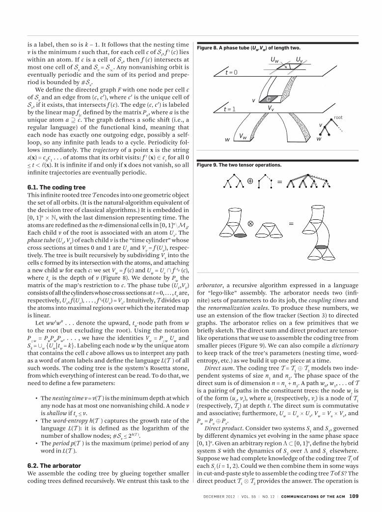
6.1. the coding treeThis infinite rooted tree T encodes into one geometric object the set of all orbits. (It is the natural-algorithm equivalent of the decision tree of classical algorithms.) It is embedded in [0, 1]n × N, with the last dimension representing time. The atoms are redefined as the n-dimensional cells in [0, 1]n\Md. Each child v of the root is associated with an atom Uv. The phase tube (Uv, Vv) of each child v is the “time cylinder” whose cross sections at times 0 and 1 are Uv and Vv = f (Uv), respec-tively. The tree is built recursively by subdividing Vv into the cells c formed by its intersection with the atoms, and attaching a new child w for each c: we set Vw = f (c) and Uw = Uv ∩ f −tv (c), where tv is the depth of v (Figure 8). We denote by Pw the matrix of the map’s restriction to c. The phase tube (UV,VV) consists of all the cylinders whose cross sections at t = 0, . . . , tv are, respectively, Uv, f (Uv), . . . , f tv(Uv) = Vv. Intuitively, T divides up the atoms into maximal regions over which the iterated map is linear.

Let ww′w″ . . . denote the upward, tw-node path from w to the root (but excluding the root). Using the notation P≤ w = PwPw′Pw″ . . . , we have the identities Vw = P≤ w Uw and Sk = ∪w {Uw|tw = k}. Labeling each node w by the unique atom that contains the cell c above allows us to interpret any path as a word of atom labels and define the language L(T ) of all such words. The coding tree is the system’s Rosetta stone, from which everything of interest can be read. To do that, we need to define a few parameters:

• The nesting time v = v(T ) is the minimum depth at which any node has at most one nonvanishing child. A node v is shallow if tv ≤ v.

• The word-entropy h(T ) captures the growth rate of the language L(T ): it is defined as the logarithm of the number of shallow nodes; #Sv ≤ 2h(T ).

• The period p(T ) is the maximum (prime) period of any word in L(T ).

6.2. the arboratorWe assemble the coding tree by glueing together smaller coding trees defined recursively. We entrust this task to the

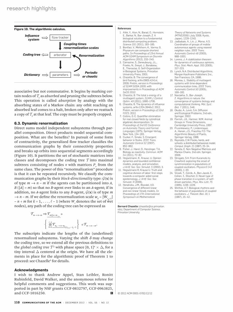
arborator, a recursive algorithm expressed in a language for “lego-like” assembly. The arborator needs two (infi-nite) sets of parameters to do its job, the coupling times and the renormalization scales. To produce these numbers, we use an extension of the flow tracker (Section 3) to directed graphs. The arborator relies on a few primitives that we briefly sketch. The direct sum and direct product are tensor-like operations that we use to assemble the coding tree from smaller pieces (Figure 9). We can also compile a dictionary to keep track of the tree’s parameters (nesting time, word-entropy, etc.) as we build it up one piece at a time.

Direct sum. The coding tree T = T1 ⊕ T2 models two inde-pendent systems of size n1 and n2. The phase space of the direct sum is of dimension n = n1 + n2. A path w0, w1, . . . of T is a pairing of paths in the constituent trees: the node wt is of the form (ut, vt), where ut (respectively, vt) is a node of T1 (respectively, T2) at depth t. The direct sum is commutative and associative; furthermore, Uw = Uu × Uv, Vw = Vu × Vv, and Pw = Pu ⊕ Pv.

Direct product. Consider two systems S1 and S2, governed by different dynamics yet evolving in the same phase space [0, 1]n. Given an arbitrary region L ⊂ [0, 1]n, define the hybrid system S with the dynamics of S2 over L and S1 elsewhere. Suppose we had complete knowledge of the coding tree Ti of each Si (i = 1, 2). Could we then combine them in some ways in cut-and-paste style to assemble the coding tree T of S? The direct product T1 ⊗ T2 provides the answer. The operation is

figure 8. a phase tube (UW,VW) of length two.

t = 0

t = 1v

v

w

root

w Vw

Vv

Uw Uv

C

figure 9. the two tensor operations.


research highlights

associative but not commutative. It begins by marking cer-tain nodes of T1 as absorbed and pruning the subtrees below. This operation is called absorption by analogy with the absorbing states of a Markov chain: any orbit reaching an absorbed leaf comes to a halt, broken only after we reattach a copy of T2 at that leaf. The copy must be properly cropped.

6.3. Dynamic renormalizationDirect sums model independent subsystems through par-allel composition. Direct products model sequential com-position. What are the benefits? In pursuit of some form of contractivity, the generalized flow tracker classifies the communication graphs by their connectivity properties and breaks up orbits into sequential segments accordingly (Figure 10). It partitions the set of stochastic matrices into classes and decomposes the coding tree T into maximal subtrees consisting of nodes v with matrices Pv from the same class. The power of this “renormalization” procedure is that it can be repeated recursively. We classify the com-munication graphs by their block-directionality type: G (x) is of type m → n − m if the agents can be partitioned into A, B (|A| = m) so that no B-agent ever links to an A-agent; if in addition, no A-agent links to any B-agent, G (x) is of type m → n − m. If we define the renormalization scale wk = |Wtk+1| − n + m for k = 1, . . . , l − 1 (where Wt denotes the set of wet nodes), any path of the coding tree can be expressed as

The subscripts indicate the lengths of the (underlined) renormalized subsystems. Varying the shift d may change the coding tree, so we extend all the previous definitions to the global coding tree T D with phase space [0, 1]n × D, for a tiny interval D centered at the origin. We have all the ele-ments in place for the algorithmic proof of Theorem 1 to proceed: see Chazelle6 for details.

acknowledgmentsI wish to thank Andrew Appel, Stan Leibler, Ronitt Rubinfeld, David Walker, and the anonymous referee for helpful comments and suggestions. This work was sup-ported in part by NSF grants CCF-0832797, CCF-0963825, and CCF-1016250.

1. Afek, Y., Alon, N., Barad, O., Hornstein, E., Barkai, N., Bar-Joseph, Z. A biological solution to a fundamental distributed computing problem. Science 331 (2011), 183–185.

2. Bonifaci, V., mehlhorn, K., Varma, g. Physarum can compute shortest paths. In Proceedings of 23rd Annual ACM-SIAM Symposium on Discrete Algorithms (2012), 233–240.

3. Camazine, S., deneubourg, J.L., Franks, N., Sneyd, J., Bonabeau, E., Theraulaz, g. Self-Organization in Biological Systems, Princeton University Press, 2001.

4. Chazelle, B. The convergence of bird flocking, arXiv:0905.4241vl, 2009. Prelim, version in Proceedings of SIAM SODA 2009, with improvements in Proceedings of ACM SoCG 2010.

5. Chazelle, B. The total s-energy of a multiagent system, SIAM J. Control Optim. 49 (2011), 1680–1706.

6. Chazelle, B. The dynamics of influence systems, arXiv:1204.3946v2, 2012. Prelim, version in Proceedings of 53rd FOCS, 2012.

7. Collins, g. E. quantifier elimination for real closed fields by cylindrical algebraic decomposition. In Proceedings of 2nd GI Conference on Automata Theory and Formal Languages (1975), Springer-Verlag, New York, 134–183.

8. Cucker, F., Smale, S. Emergent behavior in flocks. IEEE Trans. Automatic Control 52 (2007), 852–862.

9. Fisher, J., Harel, d., Henzinger, T.A. Biology as reactivity. Commun. ACM 54 (2011), 72–82.

10. Hegselmann, R., Krause, U. Opinion dynamics and bounded confidence models, analysis, and simulation. J. Artif. Soc. Soc. Simulat. 5 (2002), 3.

11. Hegselmann R, Krause U. Truth and cognitive division of labor: first steps towards a computer aided social epistemology. J. Artif. Soc. Soc. Simulat. 9 (2006).

12. Hendrickx, J.m., Blondel, V.d. Convergence of different linear and non-linear Vicsek models. In Proceedings of 17th International Symposium on Mathematical

Theory of Networks and Systems (MTNS2006) (July 2006, Kyoto, Japan), 1229–1240.

13. Jadbabaie, A., Lin, J., morse, A.S. Coordination of groups of mobile autonomous agents using nearest neighbor rules. IEEE Trans. Automatic Control 48 (2003), 988–1001.

14. Lorenz, J. A stabilization theorem for dynamics of continuous opinions. Phys. Stat. Mech. Appl. 355 (2005), 217–223.

15. Lynch, N.A. distributed Algorithms, morgan Kaufmann Publishers Inc., San Francisco, CA, 1996.

16. moreau, L. Stability of multiagent systems with time-dependent communication links. IEEE Trans. Automatic Control 50 (2005), 169–182.

17. Navlakha, S., Bar-Joseph, Z. Algorithms in nature: the convergence of systems biology and computational thinking. Mol. Syst. Biol. 7 (2011), 546.

18. Okubo, A., Levin, S.A. diffusion and Ecological Problems, 2nd edn, Springer, 2002.

19. Parrish, J.K., Hamner, W.m. Animal groups in Three dimensions, Cambridge University Press, 1997.

20. Prusinkiewicz, P., Lindenmayer, A., Hanan, J.S., Fracchia, F.d. The Algorithmic Beauty of Plants, Springer-Verlag, 1996.

21. Reynolds, C.W. Flocks, herds, and schools: a distributed behavioral model. Comput. Graph. 21 (1987), 25–34.

22. Seneta, E. Non-Negative matrices and markov Chains, 2nd edn, Springer, 2006.

23. Strogatz, S.H. From Kuramoto to Crawford: exploring the onset of synchronization in populations of coupled oscillators. Physica D 143 (2000), 1–20.

24. Vicsek, T., Czirók, A., Ben-Jacob, E., Cohen, I., Shochet, O. Novel type of phase transition in a system, of self-driven particles. Phys. Rev. Lett. 75 (1995), 1226–1229.

25. Winfree, A.T. Biological rhythms and the behavior of populations of coupled oscillators. J. Theoret. Biol. 16, 1 (1967), 15–42.

References

flow trackerInfluence system

Coupling timesrenormalization scales

Renormalization

Periodicor chaotic

Coding tree

Dictionary

arborator

parameters

figure 10. the algorithmic calculus.

Bernard Chazelle ([email protected]), department of Computer Science, Princeton University.

© 2012 ACm 0001-0782/12/12

natural algorithms and influence systemschazelle/pubs/cacm12-natalg.pdf · and influence systems by...

Documents