natural capital impacts in agriculture · supporting better bu siness decision-making natural...
TRANSCRIPT

SUPPORTING BETTER BUSINESS DECISION-MAKING
Natural Capital Impacts in Agriculture
1
Natural Capital Impacts in Agriculture
SUPPORTING BETTER BUSINESS DECISION-MAKING

The designations employed and the presentation of material in this information product do not imply
the expression of any opinion whatsoever on the part of the Food and Agriculture Organization of the
United Nations (FAO) concerning the legal or development status of any country, territory, city or area
or of its authorities, or concerning the delimitation of its frontiers or boundaries. The mention of
specific companies or products of manufacturers, whether or not these have been patented, does not
imply that these have been endorsed or recommended by FAO in preference to others of a similar
nature that are not mentioned. The views expressed in this information product are those of the
author(s) and do not necessarily reflect the views of FAO.
All rights reserved. FAO encourages the reproduction and dissemination of material in this information
product. Non-commercial uses will be authorized free of charge, upon request. Reproduction for resale
or other commercial purposes, including educational purposes, may incur fees.
Applications for permission to reproduce or disseminate FAO copyright materials, and all queries
concerning rights and licenses, should be addressed by e-mail to [email protected] or to the Chief,
Publishing Policy and Support Branch, Office of Knowledge Exchange, Research and Extension, FAO,
Viale delle Terme di Caracalla, 00153 Rome, Italy.
© FAO, June 2015
About this document
This project is led by Nadia El-Hage Scialabba, Climate, Energy and Tenure Division, with the generous
financial support of the Federal Republic of Germany. It builds on knowledge gained through the Food
Wastage Footprint: Full-Cost Accounting (FAO, 2014). With this study, FAO aims to establish the basis
for the development of the Food and Beverage Sector Guide of the Natural Capital Protocol currently in
preparation.
Acknowledgements
FAO wishes to thank Trucost staff Christopher Baldock, Elisabeth Burks and Richie Hardwicke for the
modelling work, as well as FAO colleagues Barbara Herren, Jippe Hoojeveen and Francesco Tubiello for
their expert contributions.
This project products are available at: http://www.fao.org/nr/sustainability/natural-capital

CONTENTS
Exective Summary ........................................................................................................................................ 5
Key Terms ..................................................................................................................................................... 9
Background ................................................................................................................................................. 10
Natural Capital Protocol ......................................................................................................................... 11
What is the NCP? ................................................................................................................................ 11
What are the Sector Guides?.............................................................................................................. 11
Business Engagement ......................................................................................................................... 12
Natural Capital Impacts in Agriculture ................................................................................................... 13
Phase 1: Materiality Assessment ........................................................................................................ 13
Phase 2: Trade-offs of Different Farming Systems ............................................................................. 14
PHASE 1: Materiality Assessment ............................................................................................................... 16
Methodology .......................................................................................................................................... 16
Scope .................................................................................................................................................. 16
Approach ............................................................................................................................................ 17
Quantification ................................................................................................................................. 17
Valuation......................................................................................................................................... 18
Key Findings ............................................................................................................................................ 21
Total Natural Capital Costs ................................................................................................................. 21
Crops ............................................................................................................................................... 21
Livestock ......................................................................................................................................... 29
Natural Capital Intensities .................................................................................................................. 40
Crops ............................................................................................................................................... 40
Livestock ......................................................................................................................................... 42
Regional Natural Capital Intensities ............................................................................................... 44
PHASE 2: Trade-offs of Different Farming Systems .................................................................................... 51
Value Drivers .................................................................................................................................. 51
Production costs ............................................................................................................................. 51
Overview ......................................................................................................................................... 52
Cattle Farming - Brazil ................................................................................................................................ 53
Rice Farming - India .................................................................................................................................... 58
Soybean Farming - United States of America ............................................................................................. 63

Wheat Farming - Germany ......................................................................................................................... 69
References .................................................................................................................................................. 75
Appendix I: Natural Capital Protocol .......................................................................................................... 86
Appendix II: Natural Capital Intensities per Million USD Revenue ............................................................. 87
Appendix III: Trucost’s Environmentally Extended Input-Output (EEIO) Model ........................................ 92
Appendix IV: Key Concepts Related to Natural Capital Valuations ............................................................ 96
Appendix V: Greenhouse Gas Emissions Valuation Overview ................................................................... 99
Appendix VI: Air Pollutant Valuation Overview ........................................................................................ 102
Appendix VII: Eutrophication Valuation Overview ................................................................................... 105
Appendix VIII: Ecosystem and Human Toxicity from Pesticides overview ............................................... 108
Appendix IX: Water Consumption Valuation Overview ........................................................................... 111
Appendix X: Land Use Change Valuation Overview ................................................................................. 113
Appendix XI: Greenhouse Gas Emissions from Land Clearing Overview ................................................. 116
EXECUTIVE SUMMARY
Global food production faces a challenging landscape of rising input costs, climate change, health
concerns, social inequality, resource competition and ecosystem degradation. With a global population
set to reach over 9 billion by 2050, do we fully understand the true costs and benefits associated with
different management practices of crop and livestock production?
In many countries, there is a worrying disconnect between the retail price of food and the true cost of
its production. As a consequence, food produced at great environmental cost in the form of greenhouse
gas emissions, water pollution, air pollution and habitat destruction can appear to be cheaper than
more sustainably produced alternatives.
With decisions to expand and intensify farming operations, stakeholders require better information on
the relationship between their activities, the subsequent natural capital impacts, as well as their
dependencies on natural capital. This study provides stakeholders with better information to inform
strategic decision-making, with a view to reducing impacts on natural capital that is crucial to long-term
food provisioning and improved human well-being.
To enhance the understanding of natural capital impacts and dependencies of businesses, natural
capital accounting and monetization is increasingly being used by the business community. This enables
technical environmental analysis to be translated into the language of economics and policy, so it can be
better integrated into strategic business decision-making.
This study provides stakeholders with an indication of the true magnitude of the economic and natural
capital costs associated with agricultural commodity production, and present a framework that can be
used to measure the net environmental benefits associated with different agricultural management
practices. This study builds on previous analysis from Trucost’s study for TEEB on Natural Capital at Risk:
The Top 100 Externalities of Business, and FAO’s Food Wastage Footprint: Full Cost Accounting.
To achieve this objective, Trucost has worked with FAO on two different types of analysis, utilising both
Trucost data and models, as well as FAO data, to deliver:
A global, commodity-based “materiality” approach to assess the natural capital impacts caused
by the production of four crops – maize, rice, soybean and wheat – and four livestock
commodities – beef, cattle milk, pork and poultry.
A set of four case studies focusing on different agri-commodities, exploring the trade-offs that
exist between adopting different farming practices, including:
o Beef: Holistic grazing management vs. conventional cattle grazing in Brazil
o Rice: System of rice intensification (SRI) vs. conventional rice farming in India
o Soy: Organic farming vs. conventional soybean farming in the USA
o Wheat: Organic farming vs. conventional wheat farming in Germany
It is hoped that the outputs of this analysis will further accelerate business’ uptake of a monetary
approach that supports the integration of natural capital costs into mainstream business decision-
making and operations. Furthermore, the practical case studies aim to demonstrate an approach that

assesses the natural capital cost of different management options, and how this can be used to support
better policy and to optimize production.
Within both parts of the analysis, the commodity production and environmental impact data has been
primarily sourced from FAO, with other relevant datasets coming from lifecycle analysis databases such
as Agri-footprint. The monetization of biophysical data has followed Trucost’s published methodologies
(see Appendices for details) and values the externality costs associated with different drivers of
environmental impact. This approach applies a cost to the impacts on human health, as well as
ecosystems.
MATERIALITY ASSESSMENT FINDINGS
The materiality assessment assesses impacts from the farm gate back along the upstream supply chain,
which includes the production of agricultural inputs, such as energy and feed. Downstream phases are
excluded. The main findings from this work are:
The natural capital costs associated with crop production in this study represent nearly USD
1.15 trillion, over 170 percent of its production value, whereas livestock production in this study
produces natural capital costs of over USD 1.18 trillion, 134 percent of its production value.
Farming practices have been analyzed in over 40 countries, which contribute to about 80% of
global production for each commodity, and the highest combined operational and supply chain
costs of natural capital impacts in this study have been attributed to beef production in Brazil
(USD 596 million) and the USA (USD 280 million), as well as pork production in China (USD 327
million).
On average, 64 percent of the impacts of livestock production can be attributed to operational
activities taking place on the farm. For example, the conversion of natural ecosystems to
pastureland for beef production in Brazil, which results in a natural capital cost of over USD 473
million, is the largest single impact in the study.
Supply chain impacts can represent a significant source of the costs of agricultural production,
as is the case for pork production in China, which generates air emissions, uses water, and
converts land that have a natural capital cost of over USD 118 million. This is due in part to the
production of animal feed.
On average, 77 percent of the natural capital costs of crop production occur on the farm. The
highest natural capital costs of crop production in this study can be attributed to maize farming
in China, followed by rice farming in China and India.
India generates the greatest natural capital costs associated with rice farming. The costs total
over USD 80 million and are due to the impact of water pollution, land use change and water
consumption.
In extreme cases, the overuse of fertilizers can be the source of significant natural capital
impacts, as is the case for wheat farming in Germany. The natural capital cost of fertilizer
leaching into waterways is responsible for 95 percent of its total impact, or USD 55 million.

CASE STUDY FINDINGS
Across all four studies, a number of significant benefits associated with alternative management
practices could not be monetized. These included both on-site and off-site benefits to biodiversity, soil
fertility and improved livestock welfare. The main findings from the case studies are:
Cattle Farming in Brazil
The use of holistic grazing management can result in the regeneration of grassland ecosystems,
which can reduce the cost of natural capital impacts by 11 percent.
Greenhouse gas emissions offer the most significant natural capital cost reductions through the
use of holistic grazing management: USD 1 232 per tonne of beef produced. This is due to the
increased carbon sequestration of rehabilitated grassland ecosystem on which the cattle graze.
Studies are inconclusive on the economic benefits of holistic grazing management, though one
study calculates the direct financial benefits to the farmer are around USD 68 per cow.
Rice Farming in India
Significant reductions in soil, air and water pollutants can be achieved by adopting the system of
rice intensification (SRI), with a reduction in natural capital impact of up to 97 percent, 78
percent and 16 percent respectively.
The greatest natural capital cost reductions are associated with reduced land use change (USD
48 per tonne) and water consumption (USD 41 per tonne). This is due to the increase in yields
and the use of intermittent flooding in SRI production systems.
Studies show that gross margins for SRI farms on average increase by 18 percent per hectare,
whilst operating costs decrease by 13 percent. This assumes yields of 6.5 tonnes per hectare for
SRI farms, and 3.8 tonnes for non-SRI.
Soybean Farming in the USA
Farmers that adopt organic farming practices, which utilize crop rotations and cover crops, can
achieve significant reductions in water pollution, air pollution and water consumption. The
natural capital cost-saving associated with these impacts can be, respectively, as great as USD
27, USD 19 and USD 16 per tonne of soybeans produced.
Decreasing natural capital impact is achieved through the elimination of pesticides and the
application of organic manure such as slurry.
Studies show that gross margins and operating costs for farms employing these practices
increase up to 219 percent and 12 percent per hectare, respectively. Along with the price
premium paid for organic produce, this assumes yields of 2.9 tonnes per hectare for organic
farms and 3.2 tonnes for conventional farms.
Wheat Farming in Germany
Farmers that adopt organic farming practices, which utilise crop rotations and cover crops, can
achieve significant reductions in water pollution and greenhouse gas emissions. The natural

capital cost-saving associated with these impacts can be as great as, respectively, USD 1 122 and
USD 43 per tonne of wheat produced.
Decreasing natural capital impact is achieved through the elimination of pesticide use and the
application of organic manure. Fertilizer run-off is also reduced through the use of cover crops
instead of leaving fields fallow.
Studies show that gross margins for farms employing these practices on average increase by
111 percent per hectare, whilst operating costs decrease by 32 percent. Along with the price
premium paid for organic produce, this assumes yields of 3.5 tonnes per hectare for organic
farms and 6.9 tonnes for conventional farms.
The total environmental costs calculated in this study represent an informed estimate and should be
treated with a degree of caution. This is because the calculation of non-market natural capital costs, on
a global scale, requires a number of assumptions. For example, more than 100 estimates of the social
cost of carbon are available. They run from USD -10 to USD +350 per tonne of carbon. Peer-reviewed
estimates have a mean value of USD 43 per tonne of carbon with a standard deviation of USD 83 per
tonne. For this study and in alignment with previous FAO reports, we have inflated and used the 2006
Stern cost of carbon, which equates to USD 115 per tonne.
The analysis in this report, undertaken in partnership between Trucost and FAO, will contribute to the
Natural Capital Protocol’s Food and Beverage sector guide by introducing practical examples of natural
capital valuation analysis that business can utilize.

KEY TERMS
Term Definition
Direct impacts
This refers to the operational emissions or impacts that occur due to the farming activity.
For example, the use of farm machinery that runs on diesel will cause the emission of
greenhouse gases. Also, the use of fertilizers will also cause impacts, as nutrients will enter
surrounding waterways through the process of leaching, resulting in eutrophication.
Although some impacts occur away from the farm, the impacts occur directly due to
activities that take place on the farm.
Indirect impacts
These are emissions that refer to the impacts caused by companies in the supply chains of
the farms, or those companies that subsequently use the outputs from the farm. Indirect
impacts refer to the environmental impacts that occur due to others outside the boundary
of the farm. In the context of this study, this means that all of the impacts from the
production of inputs to the farm are encompassed in the term ‘indirect impacts’.
Natural capital
Using a common definition of natural capital in the business arena, natural capital is “the
stock of natural ecosystems on Earth including air, land, soil, biodiversity and geological
resources. This stock underpins our economy and society by producing value for people,
both directly and indirectly.” (NCC, 2014a)
Natural capital intensity This refers to the monetary value of the natural capital impacts caused by each agri-sector,
per tonne of production. For example, cattle farming in South America may cause natural
capital impacts valued at USD 30 per tonne of beef produced.
Poultry
Poultry production is the term used for the production of eggs and meat. The term poultry
in this report refer to meat production only and has been used instead of the term ‘broiler’
which is “applied to chicks that have especially been bred for rapid growth.” (LEAD
Initiative, 2015)
Supply chain (downstream) This refers to entities or users of the commodity that either directly use or process the
commodity after it has left the farm.
Supply chain (upstream)
This refers to entities that supply the farm. This encompasses fertilizer and pesticide
production, and in terms of livestock production, this also includes the production of crops
as feed. The entities encompassed in this definition do not necessarily have to directly
supply the farm, but rather can be the supplier to suppliers.
In the charts of this document, where supply chain impacts have been included, if they have
not been separated into ‘1st
tier supply chain’ and ‘Rest of supply chain’, then the chart
refers to the sum of these categories. This is what is known as the ‘upstream supply chain’.
Value chain This term encompasses both upstream and downstream parts of the supply chain. Please
see above for a definition of both of these terms.
1st tier supply chain This refers to the direct suppliers to the farm. This will include companies and entities that
the farm has direct expenditure with.
Rest of supply chain On some charts, the term ‘rest of supply chain’ has been used to denote all businesses that
do not directly supply the farm. These will be companies that provide inputs into the 1st
tier
supply chain.

BACKGROUND
Businesses have a significant impact and dependency on natural capital. Impacts are caused by emitted
greenhouse gas emissions from the combustion of fossil fuels, unsustainable water abstraction in water
scarce areas, deforestation and land use change amongst others. Worryingly, business is increasingly
reliant on the very natural capital that is being degraded in order to meet the needs of a growing global
population and changing consumption patterns.
The natural capital available to business is being degraded at an ever increasing rate (UNEP 2007; UNEP
2010). Numerous international and national bodies, such as the Natural Capital Coalition1 (NCC) in the
private sector, the Wealth Accounting and the Valuation of Ecosystem Services (WAVES)2 partnership in
the public sector, and the Natural Capital Declaration3 (NCD) in the finance sector, have been formed
specifically to address the increased risk posed by the deteriorating supply-demand balance for natural
capital flows. These recent efforts have focussed on placing monetary values on natural capital in order
to factor in the effect caused by businesses and to better inform their strategic decision-making. One
such initiative that is gaining traction within the private sector, and being developed by the NCC with
support from the International Finance Corporation (IFC), the International Union for the Conservation
of Nature (IUCN) and The World Bank, is the Natural Capital Protocol.4 The objective is to create a
harmonized accounting framework, providing businesses with robust tools and metrics to identify their
impact and reliance on natural capital.
The Natural Capital Protocol consists of three main parts; the Protocol, and two sector guides; one to
cover businesses in the Food and Beverage sector, and a second for those businesses in the Apparel
value chain. The analysis in this document, undertaken in partnership between Trucost and FAO, will
contribute to the Food and Beverage sector guide by introducing practical examples of natural capital
valuation analysis that business can utilise. This study focuses on 8 agricultural commodities and
explores:
How natural capital impacts are distributed in different countries for eight commodities;
Operational versus supply chain impacts;
The monetary value of natural capital impacts;
The drivers of natural capital impacts.
Many responsible businesses are already utilizing academic research, environmental impact analysis
and datasets from organizations such as the FAO, assisting them in making more sustainable business
decisions. It is however also recognized that environmental analysis often fails to drive boardroom
decision-making, due in part to the technical language used. The Protocol and this work as part of the
Food and Beverages Sector Guide hopes to demonstrate, the value of monetizing, where possible, these
natural capital impacts and dependencies to ensure their value is understood and utilized by non-
technical, senior business decision makers. The following section provides more information on the
Natural Capital Protocol. Additional information can be found in Appendix I.
1 http://www.naturalcapitalcoalition.org/ 2 http://www.wavespartnership.org/en 3 http://www.naturalcapitaldeclaration.org/ 4 http://www.naturalcapitalcoalition.org/natural-capital-protocol.html
NATURAL CAPITAL PROTOCOL
What is the NCP?
At present, there are a growing number of fragmented activities underway regarding the valuation of
natural capital in business applications. As stated by the Natural Capital Coalition, “one of the challenges
in scaling uptake in business is the lack of a harmonized approach to enable natural capital valuation to
be practically used in these applications for example, internal management, reporting and disclosure”
(NCC, 2014b). The Natural Capital Protocol (NCP) project is a response to this challenge – with its overall
vision to transform the way business operates through understanding and incorporating their impacts
and dependencies on natural capital.
The broad aim of the NCP is to enable businesses to assess and better manage their direct and indirect
interactions with natural capital. In particular, through increasing knowledge, equipping users to
effectively link and embed outputs directly into business, for example in its operations, supply chain
management and accounting, thereby stimulating action. Table 1 provides an overview of the scope of
this study - commodities, value chain, geographies and impacts that have been included - to help
various business functions identify the relevance to their organizations. The NCP will provide clear
guidance on how businesses can assess their impacts and dependencies on natural capital, as well as
take the user through the purpose and value-add of carrying-out such an assessment within their
business.
The NCP development is being managed by a consortium led by the World Business Council for
Sustainable Development (WBCSD). The current target date for the publication of the NCP is June 2016,
while public consultation on a draft version is expected in the autumn of 2015. A rough outline of the
NCP sector guide is provided in Appendix I.
What are the Sector Guides?
In addition to the development of the Protocol, the project includes the creation of two accompanying
Sector Guides that will provide additional guidance and complementary information on implementing
the NCP in sector-specific-contexts. Initially, the Sector Guides are focussing on the Food and Beverage
and Apparel sectors due to the complexities of the natural capital impacts and dependencies across
their respective value chains. The main aim of the Sector Guides is to ensure that the NCP adequately
addresses these complexities and provides additional guidance on how a business would conduct a
natural capital assessment. Moreover, the Sector Guides will help demonstrate the business case for
natural capital measurement by coherently articulating the business value and benefits that can be
achieved by companies operating at different stages of the value chain.
The development of the Sector Guides for Food and Beverage and Apparel sectors is being led by the
International Union for Conservation of Nature (IUCN), and includes consortium members: Cambridge
Institute for Sustainability Leadership (CISL),5 EY (formerly Ernst and Young),6 FAO, Trucost7 and True
5 http://www.cisl.cam.ac.uk/ 6 http://www.ey.com/ 7 http://www.trucost.com/
Price.8 In addition, numerous sector organizations are being engaged during their formulation. As
above, the current target date for the publication of the Sector Guides is March 2016, while public
consultation on draft versions is expected in the autumn of 2015.
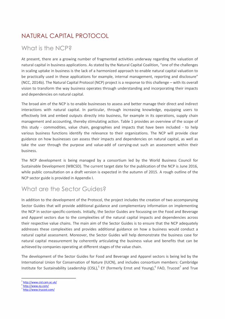
It is envisaged that the results of this study will be incorporated into two key areas of the Food and
Beverage Sector Guide – the Materiality Matrix and Practical Case Studies. The first phase of this study,
the materiality analysis across eight commodities, will help inform the Materiality Matrix. The second
part of this study will test approaches to analyzing farm-level practice/management trade-offs, and will
be utilised in the Practical Case Studies section within the Sector Guide.
FIGURE 1: VALUE DRIVERS AND THE EXPECTED BENEFITS OF USING THE NATURAL CAPITAL PROTOCOL
Business Engagement
There will also be several rounds of engagement with companies to ensure that the NCP and Sector
Guides are “fit for purpose”. Around 200 companies have been invited to become Business Engagement
Partners (BEPs) to help develop and pilot the NCP and Sector Guides. It is expected that these
companies will provide practical case studies that can be used in the main NCP and the accompanying
Sector Guides. First drafts of both publications are expected to be publically released for feedback early
in 2016.
8 http://trueprice.org/

NATURAL CAPITAL IMPACTS IN AGRICULTURE
This study, undertaken in partnership between Trucost and FAO, focuses on the natural capital impacts
caused by the production of four crop and four livestock commodities. Given the timeframes and
funding available, it was agreed to focus on the production of commodities in 40 countries, with the
countries chosen based on the production in calories per day of each commodity, as well as their
contribution to global production. The crop commodities that are included in the analysis are maize,
rice, soybean and wheat, whereas the livestock commodities that have been included are cattle (beef),
cattle (dairy), hog and pig and poultry.
The study aimed to address a number of objectives, both as a standalone piece of analysis and as a
contributor to the Food and Beverage Sector Guide as part of the Natural Capital Protocol. The study
also has the following objectives:
Improve the integration of natural capital accounting by businesses with significant operational
and agricultural supply chain impacts;
Demonstrate to businesses, using practical case studies, how natural capital impacts can be
reduced with more sustainable farm management practices.
To achieve these outcomes, the analysis was carried in two phases, utilizing Trucost data and models, as
well as FAO data and expert knowledge.
Phase 1: Materiality Assessment
A materiality study is a top-down approach that analyzes a broad set of impacts, across a broad study
area. The level of granularity and accuracy that this entails, enables the identification of a wide range of
material impacts, providing valuable insight to a wider audience. Materiality studies are often used as
an initial step to provide focus on where to undertake more robust, bottom-up analysis, relating to
production of a specific commodity in a specific location or environment.
The first phase of the study achieves this materiality approach by utilizing a mix of FAO data and
Trucost’s models to assess the natural capital impacts in monetary terms at a national level, hereafter
referred to as “natural capital costs”. This phase was developed to meet the first objective, by
identifying material impacts and presenting these impacts in a business metric: US Dollars.
Business extraction and production activities can damage natural capital with long term economic and
social consequences, which are more often paid by those affected rather than those responsible. These
risks are sufficiently large that the Word Economic Forum’s Global Risk Report (2013) cites water supply
crisis, food crises, biodiversity loss and ecosystem collapse, extreme weather events and rising
greenhouse gas emissions, within the top risks to the global economy over the next 10 years from a
likelihood and magnitude perspective. In an agricultural context, agroecological production has been
identified as one of the ways in which to regenerate agroecosystems and reverse the damage caused by
extractive production activities. Agroecology refers to the application of ecological principles in the
design and management of agricultural land and the idea of a systems-based approach viewing the
various social, technological and natural conditions that are present. It is a way of identifying the links

and interdependencies of various aspects of agricultural ecosystems so that more sustainable
production activities can be identified and implemented (Agroecology, 2015; InterDev, 2015).
This materiality study uses a top-down approach, utilizing Trucost’s environmentally extended input-
output (EEIO) model, hybridized with FAO data and Trucost’s valuation coefficients. This allows for both
the breadth and scope required for different agricultural-reliant businesses and ensures all relevant and
material natural capital impacts are identified and presented to the business user as natural capital
costs in US Dollars. Once material impacts have been identified by an agri-reliant business, they can
start to understand the scale of the risk and refine the analysis to integrate it into better internal
management practices.
An example of a similar approach taken by Trucost, covering an even broader scope, was commissioned
in 2013 by the TEEB9 for Business Coalition, now the Natural Capital Coalition, to quantify the impact on
natural capital caused by primary production and primary processing sectors in the global economy. For
each sector in each region (sector-region), the natural capital cost broken down by six key
environmental indicators: greenhouse gases (GHGs), air pollutants, water use, waste, emissions to land
and water, and land use change. The 20 sector-regions with the highest combined impacts across all
environmental indicators were also estimated. Coal power generation in Eastern Asia and North
America ranked 1st and 3rd respectively, whereas the agricultural sectors with the greatest impacts are
cattle ranching and farming in South America (2nd), followed by wheat and rice farming in Southern Asia,
which are placed 4th and 5th respectively (TEEB for Business Coalition, 2013).
The application of these materiality results resonates with a wider audience than just large private
business. For example, commodity traders and others within the finance sector can use the outputs to
engage with key commodity producers and allocate capital accordingly. The information in this analysis
will be useful in order to assess the feasibility of the long-term production of commodities and the
potential to be exposed to an increase in costs, resulting from increasing regulation or scarcity.
Regulation could take the form of making companies internalize the costs of the natural capital impacts
that they are responsible for, which can be attributed, for example, to fertilizer or pesticide use. NGOs,
food retailers and consumers also stand to benefit from this analysis, as environmental impacts that
couldn’t previously be reconciled, now have a common metric with which to be compared and
aggregated. It provides all stakeholders with a baseline to further investigate the natural capital costs
and geographies that are most material to them. It also provides a solid foundation in which to refine
the analysis in Phase 2.
Phase 2: Trade-offs of Different Farming Systems
Once a business or organization has identified the material natural capital impacts and risks, one of the
next steps is to understand how they can start to reduce those impacts, thus optimizing performance. A
practical approach is to explore the impacts of more sustainable management practices of that
particular commodity, and to then support a change through investments in technology, knowledge
sharing, infrastructure and learning.
9 The Economics of Ecosystems and Biodiversity (TEEB): www.teebweb.org
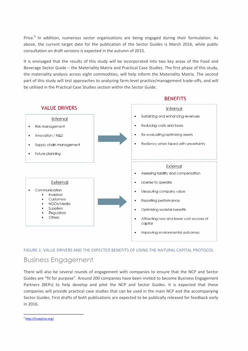
For this phase of the study, four case studies analyzed various farm-level management practices. The
analysis explored the trade-offs that exist between adopting different farming practices of selected
commodities in different countries. The analysis has considered the change in yields of each crop, as
well as natural capital costs of the impacts associated with each practice. Each study is to serve as an
example to businesses of how, taking steer from the materiality study, they can refine the accuracy and
relevance at a more granular scale, gaining an understanding of the natural capital impacts, costs and
trade-offs that exist at a farm-level for the most material and strategically important commodities. The
agri-commodities that have been identified for this phase of the work, based on the Materiality
Assessment are shown below:
Cattle (beef): Holistic grazing management vs. conventional cattle grazing in Brazil
Rice: System of rice intensification vs. conventional rice farming in India
Soy: Organic farming vs. conventional soybean farming in USA
Wheat: Organic farming vs. conventional wheat farming in Germany
The core objective of the analysis is to demonstrate to agri-businesses that by measuring its impact, and
indirectly its dependency on natural capital, this can inform more sustainable farming decisions,
increase profitability and ensure a more resilient and stable supply of each commodity. It is envisaged
that the outputs from these examples can be used by many different businesses within the food and
beverage value chain.
PHASE 1: MATERIALITY ASSESSMENT
METHODOLOGY
Scope
FAOSTAT identifies more than two hundred agricultural commodities produced in the world (FAOSTAT,
2014a). The selection of commodities to include in the materiality assessment was based on combining
an environmental impact approach and a functional unit approach.
Environmental Impact
On the environmental side, a high-level literature review was conducted to identify the categories of
agricultural commodities that most frequently feature at the top of impact rankings. In its “Food
Wastage Footprint Summary Report” (FAO, 2013), FAO ranks the agricultural commodities with the
highest contribution to global carbon, water and land use footprints according to the food wasted.
Those with the highest carbon impacts include cereals, meat and vegetables, whereas those with the
highest water and land use impacts are cereals, fruits and milk, and then meat milk, and cereals
respectively.
The results of this study, as well as the wider impact of these commodities, are substantiated by their
inclusion in WWF’s The 2050 Criteria (2012). This report addresses 10 global commodities that are
identified as high priority due to the depth and significance of their current and potential cumulative
impacts on biodiversity, greenhouse gas emissions and water use. The sectors identified include beef,
dairy and soybean, alongside others such as aquaculture, cotton, palm oil, sugar and timber.
In a separate study focusing on water, WWF identified a list of 25 key crop-industry combinations highly
exposed to both water risks and of high economic importance; these include wheat production in India
and China, and rice production in Bangladesh and India (PRI, 2014).
Functional Unit
The selection criteria for commodities in this study combines the commodity relevance to people, which
includes its role in promoting food security, and the economy, which takes into account trade value. The
data points were taken from FAOSTAT and include daily food supply, in calories per capita per year, and
the global production value generated by crops and livestock over the course of a year (FAO, 2014b).
Interestingly, these two functional unit approaches overlapped in terms of results. Thus, the most
globally important commodities in terms of food security and the economy are the following:
Crop Commodities: maize, rice, wheat and soybean10
Livestock Commodities: pork, poultry, cattle (beef) and cattle (dairy)
10 This study took into account that soybean is an important input as feed in some livestock sectors and therefore chose this commodity over the likes of sugarcane.

The following materiality assessment assesses impacts from the farm gate back along the upstream
supply chain, which includes the production of agricultural inputs such as energy and feed. Downstream
phases are excluded. Table 1 below describes the scope of the materiality assessment.
TABLE 1: SCOPE OF THE MATERIALITY ASSESSMENT
Dimension Scope Justification
Commodities Crops: maize, rice, wheat and soybean
Livestock: pork, poultry, cattle (beef) and
cattle (dairy)
Agricultural commodities with the highest contribution to
global calories produced for human consumption (FAO,
2014b) and global production value.
Value chain From production inputs to the farm gate. Paucity of data on the rest of the value chain considering the
geographical coverage and level of granularity expected.
Geographies For each commodity, the assessment
covered countries representing 80% of
global production.
Considering that environmental impacts vary amongst
countries, the assessment should include several countries
and should be based on country-specific factors where
possible. The countries contributing to the top 80% of global
production is applied due to a disproportionately large
number of countries contributing to the remaining 20%.
Environmental
impacts
Greenhouse gases (GHGs)
Air pollutants
Water abstraction
Water pollutants
Soil pollutants
Land use change11
The range of impacts should be broad as one of the
purposes of the assessment is to identify significant
environmental impacts so that an investigation in to what
practices drive these impacts can be conducted.
Approach
The methodology used has developed an approach that quantifies environmental impacts in physical
terms (cubic metres of water use, tonnes of emissions, hectares of land converted), as well as monetary
terms (US Dollars). The analysis of direct impacts refers to the quantification of environmental impacts
resulting from onsite farming activities, whereas indirect impacts refer to the quantification of
environmental impacts resulting from upstream supply chain activities (i.e. production of agricultural
inputs).
Quantification
The main body of this assessment utilises Trucost’s Environmentally Extended Input-Output model
(EEIO model). This model quantifies environmental impacts at the farm level (direct model) and through
its entire supply chain (indirect model). Assessment of direct environmental impacts were as country
specific as possible, and the assessment of the supply chain was based on global average factors.
Appendix III provides a more detailed description of Trucost’s EEIO model.
11 Land use change considers the value of ecosystem services lost from converting the land from its natural ecosystem, to the current livestock production system. It currently considers the complete loss of provisioning, regulating and cultural ecosystem services.

Environmental impacts include greenhouse emissions and air pollutants from energy and non-energy
sources, water abstraction, water pollution from fertilizer application and soil pollution from pesticide
application, as well as land use change and greenhouse gas emissions from land clearing. Table 2
summarises the scope of the environmental impacts taken into account.
TABLE 2: ENVIRONMENTAL IMPACTS THAT HAVE BEEN QUANTIFIED IN THIS ANALYSIS
Environmental
impact
Crops Livestock
Farming Supply chain Farming Supply chain
GHGs (from energy and
non-energy sources)
Yes Yes Yes Yes
GHGs (from land clearing)
Yes Yes Yes Yes
Air pollutants Yes Yes Yes Yes
Water pollutants (from manure and
fertilizers)
Yes Yes No12
Yes
Soil pollutants (from pesticides
application)
Yes Yes N/A13
Yes
Water
consumption Yes Yes Yes Yes
Land use change Yes Yes Yes Yes
Valuation
Valuation consists of transforming physical quantities into monetary values using environmental
valuation techniques. This step enables the quantification in monetary terms of the damage caused by
pollution or natural resource extraction. In order to derive valuation coefficients, a literature review was
conducted in order to understand the magnitude of each environmental impact on receptors such as
crops, ecosystems, human health and materials. Secondary literature was used to estimate the social
cost of these impacts – natural capital valuation. These valuations reflect the impact on ecosystems and
the damage to human health. Value transfer techniques were applied to make the valuations country-
12 The emissions from animal manure are not given in the Agri-Footprint library used to calculate emissions factors for livestock production. This is because “animal manure is considered to be a residual product of the animal production systems so it does not receive part of the emissions of the animal production system when animal manure is applied… Emissions due to the management of manure on the farm are included within the system boundaries, but the emissions due to application of manure are attributed to the crop cultivation stage.” (SimaPro, 2014a) As such, manure is treated as managed waste in the direct impact of livestock production. It is also important to note that heavy metals are often found in livestock manure but data availability is limited. 13 Pesticides are not used directly in livestock production so have not been included in the analysis of the impacts caused by operations of livestock production systems.

specific. The Appendices provide an overview on each valuation methodology, as well as more
information on value transfer. Table 3 and Table 4 outline what is included in the valuation scope of
each environmental impact.
TABLE 3: ENVIRONMENTAL IMPACTS THAT HAVE BEEN GIVEN A MONETARY VALUE IN THIS ANALYSIS
Environmental impact Scope
GHGs (from energy and
non-energy sources)
Multitude of impacts, including but not limited to, changes in net agricultural
productivity, human health and property damages from increased flood risk. The GHGs
considered in this analysis include carbon dioxide, methane and nitrous oxide. The social
cost of carbon, in 2013 USD, used in this study is just under USD 115 per tonne CO2
(Stern, 2006).
GHGs (from land clearing)
The carbon stock lost due to land conversion is included in this valuation. The Direct Land
Use Change Assessment Tool developed by Blonk Consultants (2014) has been used in
this study, and the carbon stock calculations are based on IPCC rules, which has been
developed to meet PAS 2050 standards as well as be consistent with the GHG Protocol
Product and Scope 3 Accounting and Reporting Standards. The carbon stock lost due to
land clearing relates to the loss of biomass and soil organic carbon. The values are crop
and country-specific and rely on a number of data sources which include FAO and
UNFCCC. The same carbon price has been applied to GHG emissions described above.
Land conversion has been attributed to crop and livestock expansion. Therefore GHGs
from land clearing is calculated as a direct impact of crop production only, whereas for
livestock production it has been calculated as a direct impact, from livestock expansion,
and a supply chain impact, from cropland expansion used as feed.
Air Pollutants
The impacts on crop yields, water quality, timber production, human health and corrosion
of building material is calculated in this valuation. Country-specific values are used in this
study and includes impacts from the emission of SOx, NOx, PM10, VOCs and ammonia
from fuel use, fertilizer application, pesticide application, enteric fermentation and other
sources. For instance, the values used for SOx emissions range between USD 600 and USD
4 000 per tonne, whereas values for VOCs range between USD 350 and USD 2 600 per
tonne.
Water pollutants (from fertilizer application)
Eutrophication impacts on ecosystems, through decreased occurrence of species. This
valuation includes the impacts on species from the emission of nitrogen, nitrates,
phosphates, and phosphorus. Values are country-specific and can range between USD 0
and USD 82 000 per tonne for nitrates, and between USD 0 and USD 818 000 per tonne
for phosphates.
Soil pollutants (from pesticides application)
Land pollutants have toxicity impacts on human health and ecosystems. This valuation
includes the impacts of over 80 pollutants, which consists of pesticides such as atrazine,
herbicides such as Diuron and fungicides such as Folpet. Values are country-specific and
can range between USD 44 000 and USD 825 000 per tonne for Atrazine, and between
USD 38 000 and USD 721 000 per tonne for Folpet.
Water consumption
This includes the impacts on human health and ecosystems. The unit of measurement for
human health is disability adjusted life years (DALYs) and the potentially disappeared
fraction of species (PDF) for ecosystem damage. Water scarcity is a factor in the water
valuation, so countries with a higher water scarcity will have a higher cost attributed to
water consumption. Values are country-specific and can range between USD 0.14 and
USD 3 per m3.

Environmental impact Scope
Land use change
This values the ecosystem services lost from the conversion of natural ecosystems to
agricultural land, including country-specific distribution of 23 global ecosystems with a
meta-analysis and valuation of 17 different ecosystem services. The natural ecosystems
that are covered in this study include: deserts; semi-deserts; savannah; temperate natural
grasslands; tropical natural grasslands; other grasslands; floodplains; peat wetlands;
swamps and marshes; other wetlands; Mediterranean woodlands; tropical woodlands;
other woodlands; mangroves; tidal marsh; salt water wetlands; boreal/coniferous forests;
temperate deciduous forests; temperate forest general; tropical dry forests; tropical
rainforests; tropical forest general and; other forests.
GHG emissions from land clearing is included in the section above.
TABLE 4: SUMMARY OF LIMITATIONS
Limitation Explanation
Aggregation of data
In some cases, components of valuations which represent impacts on different receptors,
such as human populations, are aggregated and use different valuation techniques. The
individual components of valuations may or may not be directly comparable, but the
methodology applied is consistent across the different impact categories and to each
unique receptor.
Exclusions Some impact categories have been excluded on the basis of materiality or data availability.
Please see the relevant methodology sections in the Appendices for further information.
Overlap In some instances, where global averages have been used, or if there is a lack of data, some
aspects of the valuations may overlap in scope. If this has occurred, this is stated in the
relevant methodology section in the Appendices of this document.
Static Valuations are adjusted using inflation rates and apply at a specific point in time.
Value transfer
Value transfer has been used at points to derive valuation coefficients that have been
applied during this study. Transferring values from study sites to the policy sites can contain
a number of errors, for example, the value at the policy site can only be as accurate as the
original calculation. Also, all of the limitations surrounding the original study are equally
valid for the value at the policy site. See Brander (2013) for a comprehensive assessment of
value transfer techniques.
MAIN FINDINGS
Total Natural Capital Costs
This section describes the impacts on natural capital in terms of the total costs caused by the annual
production of each commodity in each study country. Intensities are used in conjunction with annual
production quantities in order to calculate the total natural capital costs per country. Please refer to the
Appendix III for more information on how intensities and costs of natural capital impacts have been
calculated in Trucost’s environmentally-extended input-output (EEIO) model.
The results are broken down by direct operations (on-site farming activities), the first tier of the supply
chain (businesses who directly supply the farms), and by the rest of the supply chain (the suppliers of
the suppliers). In the case of crop farming, first tier suppliers include, but are not limited to, energy
providers, as well as pesticide and fertilizer manufacturers. For livestock sectors, in this instance, first
tier suppliers include feed producers, such as those in maize and soybean farming, as well as energy
providers.
As described in the Approach section, the quantification of impacts was based on country-specific
factors where possible, or global average factors if not. Valuation factors are country-specific, apart
from greenhouse emissions where the impact on natural capital is global. However, country-specific
valuations have limitations, such as the fact that they rely on national averages, or that the dispersion
models used are not country-specific. The analysis that is contained hereafter should be used to
highlight where there are opportunities to improve farming practices, and not to directly compare
impacts in different countries without further analysis. This is because of the detailed nuances that exist
between farming practices, as presented in Phase 2.
Crops
Figure 2 shows each of the four crops, in order of the highest combined operational and supply chain
natural capital costs per unit of production, across the globe.
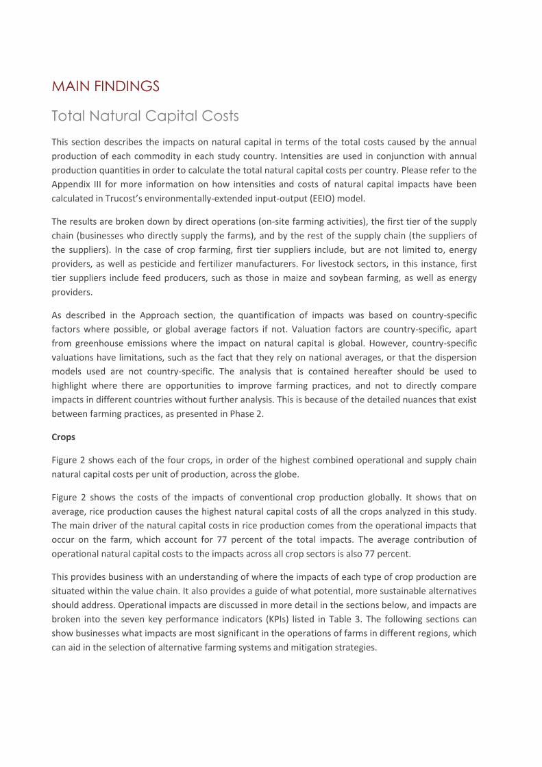
Figure 2 shows the costs of the impacts of conventional crop production globally. It shows that on
average, rice production causes the highest natural capital costs of all the crops analyzed in this study.
The main driver of the natural capital costs in rice production comes from the operational impacts that
occur on the farm, which account for 77 percent of the total impacts. The average contribution of
operational natural capital costs to the impacts across all crop sectors is also 77 percent.
This provides business with an understanding of where the impacts of each type of crop production are
situated within the value chain. It also provides a guide of what potential, more sustainable alternatives
should address. Operational impacts are discussed in more detail in the sections below, and impacts are
broken into the seven key performance indicators (KPIs) listed in Table 3. The following sections can
show businesses what impacts are most significant in the operations of farms in different regions, which
can aid in the selection of alternative farming systems and mitigation strategies.

FIGURE 2: GLOBAL OPERATIONAL AND SUPPLY CHAIN NATURAL CAPITAL COSTS PER TONNE OF CROP
PRODUCTION
Figure 3 shows the costs of the top 10 crop production impacts with the highest natural capital costs by
country. It shows that the total impact associated with the production of maize and rice in China have
the greatest natural capital impact. China is the largest producer of rice, and is the second largest
producer of maize behind the United States of America, which produces almost 40 percent more maize
than China. China’s rice production inflicts greater natural capital costs than rice production in India
despite China’s natural capital cost per tonne of rice production being 21 percent. This is driven by the
greater production volume of rice in China. Brazil is the only producer of soybeans to feature in the list
and this is mainly due to the impacts of land use change that occur as a result of its operations.
Operational impacts account for 85 percent of Brazil’s soybean farming total impacts. In total, the top
10 countries and sectors listed in Figure 3, account for 59 percent of the total crop production natural
capital costs in this study.
FIGURE 3: TOP 10 OPERATIONAL AND SUPPLY CHAIN NATURAL CAPITAL COSTS OF CROP PRODUCTION
BY COUNTRY

Figure 3 builds on the information presented above to highlight to business the specific sectors and
countries with the largest cost of environmental impacts during crop production. It highlights significant
global issues and provides an indication of the sustainability of conventional farming systems.
Businesses can use this as a starting point to investigate what impacts are most material in these sectors
and countries, then qualitatively assess whether the external costs of the impacts are likely to be
internalised, and over what timescales. Businesses can use this information to either identify what
impacts alternative farming systems should address, so as to reduce these impacts, or can use this
information to assess to what degree they are dependent on the natural capital that they are impacting.
Table 5 outlines the top 3 contributors to the natural capital costs in each crop production sector in the
study. The natural capital costs include both operational and supply chain impacts.
TABLE 5: TOP CONTRIBUTORS TO THE NATURAL CAPITAL COSTS IN EACH CROP SECTOR
(OPERATIONAL AND SUPPLY CHAIN IMPACTS)
Crop
Top contributors to the natural capital costs (USD million) Total costs
(USD million) 1st 2nd 3rd
Maize China
129 607 (35%)
USA
89 687 (24%)
Brazil
57 344 (16%) 369 243
Rice China
113 681 (22%)
India
113 315 (22%)
Indonesia
62 580 (12%) 507 308
Soybean Brazil
102 268 (58%)
USA
52 051 (30%)
Argentina
21 724 (12%) 176 044
Wheat China
84 602 (19%)
India
69 387 (16%)
Germany
61 560 (14%) 439 188
The breakdown of these results, for all countries in the study, can be seen from Figure 4 to Figure 7, and
in
Table 6. The figures show the natural capital costs associated with the production of each of the crops in
this study, in conjunction with the total production of each crop.

FIGURE 4: OPERATIONAL AND SUPPLY CHAIN NATURAL CAPITAL COSTS OF MAIZE PRODUCTION BY
COUNTRY
Findings
China and the USA have the highest impact on natural capital due to maize production. Together, they are responsible for 59 percent of the total natural capital costs in this sector for the countries analyzed.
Land use change and the emission of water pollutants cause the greatest natural capital impact in this sector. Land use change means that ecosystem services are lost, which provide benefits directly to people and businesses. Fertilizers are a common cause of water pollution and a major source of natural capital impact in this study.
This highlights to business that capacity of ecosystem services to support agricultural ecosystems are decreasing. A high conversion rate from naturally occurring land to man-made ecosystems indicate that the base of natural capital that they rely on is being degraded. The degree of a business’ dependency on those ecosystem services will dictate the costs of degradation to that business, as well as the rate of internalisation of those costs.

FIGURE 5: OPERATIONAL AND SUPPLY CHAIN NATURAL CAPITAL COSTS OF RICE PRODUCTION BY
COUNTRY
Findings
China and India have the highest impact on natural capital due to rice production in this study. Each country is responsible for 22 percent of the natural capital costs caused due to rice production. China and India are also responsible for 62 percent of the production of rice of countries in this study.
The cost of natural capital impacts in the study countries are driven by a combination of land use change, the emissions of water pollutants, and water consumption. In each country, these impacts are responsible for over 93 percent of the impacts.
These results show businesses that the capacity of ecosystem services and functions to support the environment, and agricultural production, are decreasing. It also highlights that water pollution, from the application of fertilizers, also has a significant impact on species that provide a supporting service to ecosystem service provision. For businesses to reduce their impact on ecosystems, and hence increase their resilience, addressing the negative effects of fertilizers and the conversion of land should be a priority.

FIGURE 6: OPERATIONAL AND SUPPLY CHAIN NATURAL CAPITAL COSTS OF SOYBEAN PRODUCTION BY
COUNTRY
Findings
Brazil is responsible for 58 percent of the natural capital impacts in the soybean farming sector in this study. The USA, on the other hand, produces 11 percent more soybeans, but with almost half the impact of Brazilian producer. This is despite the fact that less land is required to produce a tonne of soybean in the USA.
The majority of the natural capital impacts occurring due to the production of soybeans in Brazil is because of land use change (63 percent) and water pollution (23 percent). This is a significant impact as ecosystem services are lost when areas, such as the Amazon Rainforest and Cerrado, are cleared to make way for soybean plantations.
Businesses should be aware that the impacts due to land use change and water pollution decrease the capacity of ecosystems to support agricultural production in these regions. The cost of these impacts could be realised through an increased variability in yield due to a change in local environmental conditions, such as the availability of good quality irrigation water. The identification of the type and magnitude of impacts allows businesses to select mitigation strategies that directly address the most material environmental issues.

FIGURE 7: OPERATIONAL AND SUPPLY CHAIN NATURAL CAPITAL COSTS OF WHEAT PRODUCTION BY
COUNTRY
Findings
The top three countries in this study, China, India and Germany, are responsible for almost 50 percent of the cost of the impacts on natural capital in this sector globally. China and India are the two largest producers of wheat, and are therefore expected to have higher impact on natural capital. However, Germany is ranked 9th in terms of total wheat production, and generates a disproportionately high impact on natural capital.
The high natural capital costs associated with growing wheat in Germany are due to the water pollution caused by fertilizer application on the farm – 95 percent of its total impact. The European Environmental Agency (EEA) identifies Germany one of the countries in Europe with the greatest exceedance of critical nutrient loads (EEA, 2014). Conversely, the impacts caused by wheat production in China and India, are due to land use change and water consumption respectively.
These geo-specific impacts outline to businesses that the dependency on water availability in China and India is a key factor when considering more sustainable farming systems. Whereas the use of fertilizers, and their impact on water quality and ecosystems, should be a focus for businesses in Germany.

TABLE 6: TOTAL NATURAL CAPITAL COSTS OF CROP PRODUCTION (USD PER COUNTRY)
Rank Country
Operational Supply chain (tier 1) Rest of supply chain Production quantity
Cost
(USD million) %
Cost
(USD million) %
Cost
(USD million) %
tonnes %
Maize production
1 China 94 880 36% 19 674 33% 15 053 33% 193 000 000 28%
2 USA 46 806 18% 24 294 41% 18 587 41% 314 000 000 45%
3 Brazil 49 352 19% 4 528 8% 3 464 8% 55 700 000 8%
4 France 23 228 9% 1 309 2% 1 002 2% 15 900 000 2%
5 Indonesia 14 754 6% 2 387 4% 1 826 4% 17 600 000 3%
6 Mexico 12 361 5% 1 842 3% 1 410 3% 17 600 000 3%
7 India 9 959 4% 1 335 2% 1 022 2% 21 800 000 3%
8 Ukraine 8 952 3% 1 241 2% 950 2% 22 800 000 3%
9 Argentina 3 428 1% 1 331 2% 1 018 2% 23 800 000 3%
10 Canada 1 822 1% 810 1% 620 1% 10 700 000 2%
- Total 265 484 100% 58 751 100% 44 951 100% 692 900 000 100%
Rice production
1 China 70 218 18% 23 905 37% 19 558 37% 201 000 000 35%
2 India 80 245 21% 18 188 28% 14 881 28% 158 000 000 27%
3 Indonesia 48 647 13% 7 664 12% 6 270 12% 65 700 000 11%
4 Thailand 49 999 13% 4 275 7% 3 498 7% 34 600 000 6%
5 Viet Nam 49 496 13% 3 945 6% 3 228 6% 42 400 000 7%
6 Bangladesh 48 591 13% 3 056 5% 2 500 5% 50 600 000 9%
7 Myanmar 38 740 10% 3 523 5% 2 882 5% 29 000 000 5%
- Total 385 247 100% 64 555 100% 52 817 100% 581 300 000 100%
Soybean production
1 Brazil 89 035 63% 9 335 38% 3 898 38% 74 800 000 36%

Rank Country
Operational Supply chain (tier 1) Rest of supply chain Production quantity
Cost
(USD million) %
Cost
(USD million) %
Cost
(USD million) %
tonnes %
2 USA 37 027 26% 10 599 44% 4 425 44% 84 200 000 41%
3 Argentina 15 460 11% 4 419 18% 1 845 18% 48 900 000 24%
- Total 139 534 100% 24 353 100% 10 168 100% 207 900 000 100%
Wheat production
1 China 62 504 18% 12 870 25% 9 228 25% 117 000 000 21%
2 India 56 312 16% 7 615 15% 5 460 15% 86 900 000 16%
3 Germany 57 723 16% 2 235 4% 1 603 4% 22 800 000 4%
4 France 47 869 14% 3 307 6% 2 371 6% 38 000 000 7%
5 Pakistan 32 269 9% 3 005 6% 2 155 6% 25 200 000 5%
6 Russia 17 538 5% 3 340 7% 2 395 7% 56 200 000 10%
7 USA 14 103 4% 4 935 10% 3 538 10% 54 400 000 10%
8 Turkey 16 604 5% 2 617 5% 1 877 5% 21 800 000 4%
9 Ukraine 9 455 3% 1 273 2% 913 2% 22 300 000 4%
10 Poland 9 213 3% 886 2% 635 2% 9 339 200 2%
11 Iran 8 044 2% 1 454 3% 1 043 3% 13 500 000 2%
12 Australia 5 741 2% 2 476 5% 1 775 5% 27 400 000 5%
13 United Kingdom 5 355 2% 1 527 3% 1 095 3% 15 300 000 3%
14 Kazakhstan 4 958 1% 1 533 3% 1 099 3% 22 700 000 4%
15 Canada 3 737 1% 2 040 4% 1 463 4% 25 300 000 5%
- Total 351 339 100% 51 113 100% 36 651 100% 558 139 200 100%
Livestock
Figure 8 shows each of the four types of livestock, in order of the highest combined operational and
supply chain natural capital costs per unit of production globally. It is important to note that operational
impacts due to water pollution and soil pollution have not been included in the analysis below. However,
emissions due to the management of manure on the farm are included, but the emissions due to
application of manure are attributed to the crop cultivation stage. As such, manure is treated as
managed waste in the direct impact of livestock production. It is also important to note that heavy
metals are often found in livestock manure but data availability is limited. The integration of these
impacts would increase the natural capital costs of livestock production.

FIGURE 8: OPERATIONAL AND SUPPLY CHAIN NATURAL CAPITAL COSTS OF LIVESTOCK PRODUCTION14
Figure 8 shows that on average, the production of beef causes the highest natural capital costs of all the
livestock sectors analyzed in this study. The main driver of the natural capital costs in beef production
comes from the operational impacts, which account for 75 percent of the total impacts. Conversely, the
majority of the impacts of poultry production occur in the supply chain, which are responsible for 73
percent of the impacts. Overall, the average contribution of the operational impacts to the total natural
capital costs, across all sectors, is 71 percent, meaning that the cost of supply chain impacts, account for
29 percent.
Figure 8 shows the costs of the impacts of conventional livestock production globally. This provides
business with an understanding of where the impacts of each type of livestock are situated within the
value chain. It also provides a guide of what potential, more sustainable alternatives, should address.
Operational impacts are discussed in more detail in the sections below. The following sections can show
businesses what impacts are most significant in the operations of farms in different regions, which can
aid in the selection of alternative farming systems and mitigation strategies.
Figure 9 shows the top 10 livestock production impacts with the highest natural capital costs by country.
14 It is important to remember that the operational natural capital costs associated with livestock production do not include the water pollution impacts occurring due to manure.
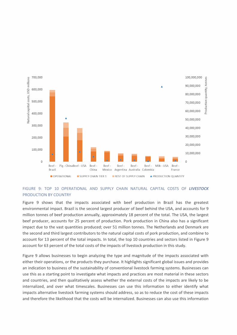
FIGURE 9: TOP 10 OPERATIONAL AND SUPPLY CHAIN NATURAL CAPITAL COSTS OF LIVESTOCK
PRODUCTION BY COUNTRY
Figure 9 shows that the impacts associated with beef production in Brazil has the greatest
environmental impact. Brazil is the second largest producer of beef behind the USA, and accounts for 9
million tonnes of beef production annually, approximately 18 percent of the total. The USA, the largest
beef producer, accounts for 25 percent of production. Pork production in China also has a significant
impact due to the vast quantities produced; over 51 million tonnes. The Netherlands and Denmark are
the second and third largest contributors to the natural capital costs of pork production, and combine to
account for 13 percent of the total impacts. In total, the top 10 countries and sectors listed in Figure 9
account for 63 percent of the total costs of the impacts of livestock production in this study.
Figure 9 allows businesses to begin analyzing the type and magnitude of the impacts associated with
either their operations, or the products they purchase. It highlights significant global issues and provides
an indication to business of the sustainability of conventional livestock farming systems. Businesses can
use this as a starting point to investigate what impacts and practices are most material in these sectors
and countries, and then qualitatively assess whether the external costs of the impacts are likely to be
internalized, and over what timescales. Businesses can use this information to either identify what
impacts alternative livestock farming systems should address, so as to reduce the cost of these impacts
and therefore the likelihood that the costs will be internalized. Businesses can also use this information

to begin to assess to what degree they are dependent on the natural capital that they are impacting,
and how the change of these costs can materially affect the business. Table 7 shows the top 3 three
ountries, in each livestock sector, that impact most on natural capital.
TABLE 7: TOP CONTRIBUTORS TO THE NATURAL CAPITAL COSTS IN EACH LIVESTOCK SECTOR
(OPERATIONAL AND SUPPLY CHAIN IMPACTS)
Livestock Top contributors to the natural capital costs (USD million) Total costs
(USD million)
1st
2nd
3rd
Cattle (beef) Brazil
595 987 (36%)
USA
279 758 (17%)
China
120 961 (7%) 1 668 618
Cattle (dairy) USA
44 948 (16%)
Brazil
31 969 (12%)
India
27 317 (10%) 274 560
Pork China
326 677 (62%)
Netherlands
35 326 (7%)
Denmark
29 689 (6%) 523 470
Poultry USA
29 817 (19%)
Brazil
27 904 (15%)
China
27 606 (14%) 188 704
Operational and supply chain impacts for these livestock sectors are discussed in more detail in the
Figures to 13 and Table 8 below.

FIGURE 10: OPERATIONAL AND SUPPLY CHAIN NATURAL CAPITAL COSTS OF CATTLE (BEEF)
PRODUCTION BY COUNTRY
Findings
Brazil has the greatest impact on natural capital due to beef production. The impacts are mainly due to land use change and the impact of greenhouse gas emissions. Combined, these impacts represent 99 percent of the costs of the impacts for Brazilian beef production. The USA also has a significant impact on natural capital due to beef production, and the combined costs due to land use change and greenhouse gas emissions represent 92 percent of the impacts.
This demonstrates to businesses that the expansion of livestock on naturally occurring ecosystems can significantly degrade their capacity to deliver ecosystem services. This could directly impact cattle farmers, or these effects could indirectly affect other farming practices in the region by changing water availability and rates of soil erosion. Businesses can use this information as a starting point to analyze which type of impacts they are directly and indirectly exposed to. This can be performed in terms of analysing the extent to which the farm is dependent on the natural capital being degraded, and how the business may have to adapt to these changes.

FIGURE 11: OPERATIONAL AND SUPPLY CHAIN NATURAL CAPITAL COSTS OF CATTLE (DAIRY)
PRODUCTION BY COUNTRY
Findings
The USA, Brazil and India account for 38 percent of the costs of the impacts due to milk production in this study. Typically around 70 percent of these impacts are due to land use change by converting naturally occurring ecosystems, such as rainforest, to pastureland. The top 10 countries in this study account for 70 percent of the milk production and natural capital costs in this study.
This highlights to business that capacity of ecosystem services to support agricultural ecosystems are decreasing. A high conversion rate from naturally occurring land to man-made ecosystems indicates that the base of natural capital that they rely on is being degraded. The degree of a business’ dependency on those ecosystem services will dictate the costs of degradation to that business, as well as the rate of internalisation of those costs. Businesses should also be aware that 25 percent of the costs of milk production are due to greenhouse gas emissions. The internalisation of the costs of carbon emissions could begin to impact as regulatory bodies look to curtail GHG emissions coming from agriculture.

FIGURE 12: OPERATIONAL AND SUPPLY CHAIN NATURAL CAPITAL COSTS OF PORK PRODUCTION BY
COUNTRY
Findings
China is responsible for 60 percent of the natural capital costs of the pork production in this study and is responsible for 58 percent of the production. Other significant contributors to global natural capital costs include the Netherlands (9 percent) and Denmark (8 percent).
The overwhelming majority of the operational impacts from pork production are due to land use change, which account for 88 percent of the total. However, supply chain impacts of pork production are also a significant source of natural capital costs. For example, in China, land use change, largely due to the production of feed, accounts for 30 percent of the supply chain impact, and greenhouse gas emissions account for an additional 28 percent.
This information gives businesses and other stakeholder’s insight into the dependency of pork producers in China of purchasing concentrate feeds. This allows businesses to start assessing whether their operations, or their suppliers, could be affected by the natural capital impacts associated with the production of feed. It also enables businesses to start assessing whether pork production can continue to expand in China, or whether other farming systems would need to be adopted to increase supply.

FIGURE 13: OPERATIONAL AND SUPPLY CHAIN NATURAL CAPITAL COSTS OF POULTRY PRODUCTION BY
COUNTRY
Findings
The top three contributors to the natural capital costs in this study, the USA, Brazil, and China are responsible for 48 percent of the natural capital costs of poultry production. Together, they also represent 57 percent of poultry production analyzed. In general, 72 percent of the natural capital impacts occur in the supply chain.
Typically, the supply chain impacts of poultry production are mainly due to the emissions of land use change, greenhouse gas emissions, and air pollution, which combine to contribute over 83 percent of the supply chain natural capital costs.
The USA creates natural capital impacts that are 23 percent greater than those in Brazil. The operational natural capital costs is driven by the emission of greenhouse gases and air pollutants. The greenhouse gas impacts in the supply chain are mainly driven by the manufacture of feed. Interestingly, Indonesia inflicts high natural impacts proportional to its production. The natural capital cost of its impacts are USD 7 000 per tonne, which is over three-times higher than USA and China. In part, this is due to the operational GHG emissions in Indonesia, which are nearly four-times higher than the USA.

37
TABLE 8: TOTAL NATURAL CAPITAL COSTS OF LIVESTOCK PRODUCTION (USD PER COUNTRY)
Rank Country
Operational Supply chain (tier 1) Rest of supply chain Production quantity
Cost
(USD million) %
Cost
(USD million) %
Cost
(USD million) %
tonnes %
Cattle (beef) production
1 Brazil 542 363 43% 28 829 13% 19 517 12% 9 030 000 18%
2 USA 178 918 14% 56 530 25% 41 365 26% 12 000 000 25%
3 China 84 648 7% 19 719 9% 13 612 8% 6 182 155 13%
4 Mexico 78 242 6% 6 392 3% 4 350 3% 1 803 930 4%
5 Argentina 49 841 4% 11 276 5% 7 912 5% 2 419 700 5%
6 Australia 49 112 4% 9 054 4% 6 416 4% 2 109 860 4%
7 Colombia 41 071 3% 4 035 2% 2 813 2% 940 000 2%
8 France 22 796 2% 9 548 4% 6 694 4% 1 501 610 3%
9 Russian Federation 19 876 2% 10 066 4% 7 000 4% 1 625 470 3%
10 Japan 11 175 1% 13 411 6% 10 005 6% 500 440 1%
11 Canada 21 913 2% 6 742 3% 4 934 3% 1 154 240 2%
12 Venezuela 30 906 2% 1 530 1% 1 057 1% 494 500 1%
13 Turkey 11 716 1% 7 627 3% 5 680 4% 644 906 1%
14 Germany 12 914 1% 6 946 3% 4 846 3% 1 170 380 2%
15 United Kingdom 12 507 1% 5 560 2% 3 899 2% 936 000 2%
16 Uzbekistan 12 511 1% 3 429 2% 2 503 2% 763 000 2%
17 South Africa 12 165 1% 3 472 2% 2 536 2% 828 609 2%
18 Italy 7 511 1% 5 995 3% 4 246 3% 1 000 370 2%
19 Pakistan 12 652 1% 2 793 1% 1 958 1% 761 000 2%
20 Ireland 9 128 1% 3 329 1% 2 325 1% 545 942 1%
21 Egypt 9 454 1% 2 899 1% 2 138 1% 454 484 1%
22 New Zealand 6 581 1% 2 223 1% 1 561 1% 622 676 1%
23 Uruguay 6 701 1% 2 080 1% 1 448 1% 479 000 1%
24 Spain 5 910 0% 1 905 1% 1 269 1% 604 113 1%
25 Poland 5 661 0% 1 899 1% 1 276 1% 394 900 1%
- Total 1 256 096 100% 227 287 100% 161 358 100% 48 967 285 100%

Rank Country
Operational Supply chain (tier 1) Rest of supply chain Production quantity
Cost
(USD million) %
Cost
(USD million) %
Cost
(USD million) %
tonnes %
Cattle (dairy) production
1 USA 24 463 15% 7 101 18% 13 034 18% 89 000 000 18%
2 Brazil 23 892 15% 2 801 7% 5 074 7% 32 100 000 7%
3 India 18 622 12% 3 015 8% 5 507 8% 52 500 000 11%
4 China 11 590 7% 3 300 8% 5 987 8% 36 900 000 8%
5 Russian Federation 9 766 6% 2 758 7% 4 968 7% 31 400 000 6%
6 Germany 6 038 4% 2 576 6% 4 753 7% 30 300 000 6%
7 France 5 317 3% 2 172 5% 3 859 5% 24 400 000 5%
8 New Zealand 4 242 3% 1 649 4% 3 021 4% 17 900 000 4%
9 Mexico 6 334 4% 782 2% 1 405 2% 10 700 000 2%
10 Iran 6 224 4% 445 1% 830 1% 6 391 400 1%
11 Turkey 3 790 2% 1 161 3% 2 169 3% 13 800 000 3%
12 Poland 3 728 2% 945 2% 1 674 2% 12 400 000 3%
13 Japan 1 930 1% 1 498 4% 2 779 4% 7 474 310 2%
14 United Kingdom 2 850 2% 1 133 3% 1 999 3% 14 200 000 3%
15 Uzbekistan 3 939 2% 547 1% 1 023 1% 6 712 200 1%
16 Italy 2 218 1% 1 153 3% 2 073 3% 10 500 000 2%
17 Canada 2 133 1% 1 124 3% 2 086 3% 8 400 000 2%
18 Pakistan 3 316 2% 662 2% 1 204 2% 12 900 000 3%
19 Colombia 3 497 2% 568 1% 1 023 1% 7 500 000 2%
20 Ukraine 2 721 2% 768 2% 1 354 2% 10 800 000 2%
21 Australia 2 748 2% 709 2% 1 291 2% 9 101 000 2%
22 Argentina 2 596 2% 707 2% 1 265 2% 10 500 000 2%
23 Netherlands 1 711 1% 1 023 3% 1 817 2% 11 600 000 2%
24 Ecuador 2 357 1% 469 1% 843 1% 6 375 320 1%
25 Belarus 1 971 1% 424 1% 744 1% 6 489 300 1%
26 Spain 1 176 1% 521 1% 918 1% 6 522 000 1%
- Total 158 930 100% 40 012 100% 72 700 100% 480 376 230 100%
Pork production

Rank Country
Operational Supply chain (tier 1) Rest of supply chain Production quantity
Cost
(USD million) %
Cost
(USD million) %
Cost
(USD million) %
tonnes %
1 China 208 328 60% 44 647 67% 46 014 70% 51 500 000 58%
2 Netherlands 32 357 9% 1 108 2% 923 1% 1 347 170 2%
3 Denmark 26 734 8% 1 104 2% 937 1% 1 720 200 2%
4 Germany 19 670 6% 3 071 5% 2 507 4% 5 616 070 6%
5 Philippines 19 979 6% 1 425 2% 1 222 2% 1 649 300 2%
6 USA 10 202 3% 4 620 7% 4 910 7% 10 300 000 12%
7 Brazil 11 072 3% 2 052 3% 1 350 2% 3 227 000 4%
8 Spain 6 944 2% 1 982 3% 1 526 2% 3 469 350 4%
9 Russian Federation 3 003 1% 2 295 3% 2 572 4% 2 427 640 3%
10 France 3 750 1% 1 251 2% 1 011 2% 2 157 410 2%
11 Viet Nam 2 015 1% 2 043 3% 1 760 3% 3 098 900 4%
12 Canada 2 076 1% 1 146 2% 1 258 2% 1 953 550 2%
- Total 345 968 100% 66 745 100% 65 988 100% 88 466 590 100%
Poultry production
1 USA 9 632 19% 12 250 20% 14 636 20% 17 100 000 24%
2 Brazil 6 689 13% 10 074 16% 11 141 15% 11 000 000 15%
3 China 8 785 17% 9 349 15% 8 925 12% 12 100 000 17%
4 Indonesia 3 349 6% 3 010 5% 4 942 7% 1 613 600 2%
5 Russian Federation 2 152 4% 2 059 3% 3 728 5% 2 909 430 4%
6 Iran 2 110 4% 2 287 4% 3 205 4% 1 686 000 2%
7 Mexico 2 013 4% 2 608 4% 2 961 4% 2 765 020 4%
8 India 2 282 4% 2 333 4% 2 372 3% 2 206 000 3%
9 Japan 1 134 2% 1 809 3% 2 598 3% 1 382 000 2%
10 South Africa 1 455 3% 1 560 3% 1 828 2% 1 485 610 2%
11 Turkey 1 195 2% 1 576 3% 1 762 2% 1 613 310 2%
12 Colombia 845 2% 1 336 2% 1 826 2% 1 086 000 2%
13 Malaysia 956 2% 1 269 2% 1 509 2% 1 315 000 2%
14 Thailand 1 163 2% 1 121 2% 1 246 2% 1 257 600 2%
15 Peru 762 1% 1 187 2% 1 511 2% 1 084 820 2%

Rank Country
Operational Supply chain (tier 1) Rest of supply chain Production quantity
Cost
(USD million) %
Cost
(USD million) %
Cost
(USD million) %
tonnes %
16 Myanmar 1 172 2% 1 082 2% 1 109 1% 1 015 860 1%
17 Argentina 854 2% 1 291 2% 1 203 2% 1 649 000 2%
18 Canada 750 1% 1 008 2% 1 440 2% 1 053 220 1%
19 France 922 2% 782 1% 1 241 2% 1 112 140 2%
20 United Kingdom 869 2% 821 1% 1 234 2% 1 354 000 2%
21 Spain 734 1% 840 1% 1 329 2% 1 205 750 2%
22 Australia 643 1% 805 1% 1 106 1% 1 017 090 1%
23 Poland 755 1% 635 1% 1 082 1% 1 150 000 2%
24 Germany 733 1% 659 1% 1 063 1% 895 880 1%
- Total 51 955 100% 61 749 100% 75 000 100% 71 057 330 100%
Natural Capital Intensities
The natural capital intensity represents the average impact on natural capital caused by the production
of one tonne of each commodity, each year. The average intensity is shown first at a global level, and
then at a continental level. The intensities are representative of all countries in this study (80 percent of
global production for each commodity), and they are weighted by the production quantity in each
country. The information in the following sections has been broken out so that the operational impacts
of the farm, and the impacts of those supplying the farm, are presented separately. These are each
referred to as operational and supply chain impacts.
Crops
Figure 14 and Figure 15 show the breakdown of natural capital impacts, per tonne of production, for
operational and supply chain impacts globally. The figures show that on average, for all crops,
operational impacts are greater than supply chain impacts per tonne of crop produced. In general, the
natural capital costs are driven by the emissions of water pollutants and the effects of land use change
on ecosystem service loss.
The information shows businesses that, when analysing the impacts of conventional crop farming
systems, and how these impacts can be reduced, focus should be on the farm’s operational impacts. In
particular, the effect of water pollution from fertilizer application, and the loss of ecosystem services
from land use change should be addressed. For instance, it was shown earlier that maize production in
Germany has a particularly high operational impact due to the leaching and subsequent eutrophication
of fertilizers in water bodies. Businesses and other stakeholders can begin to look at the application
rates of fertilizers, the method of application, and the drivers for this. This can include analyzing the
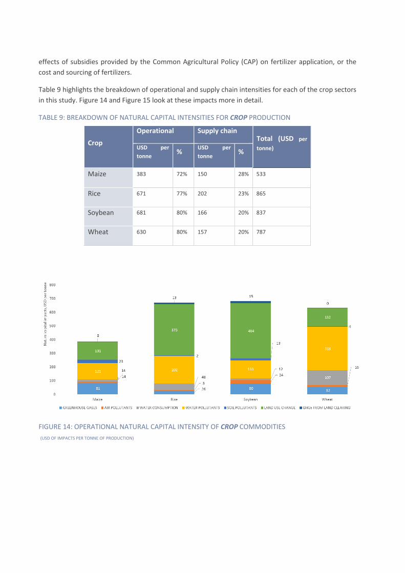
effects of subsidies provided by the Common Agricultural Policy (CAP) on fertilizer application, or the
cost and sourcing of fertilizers.
Table 9 highlights the breakdown of operational and supply chain intensities for each of the crop sectors
in this study. Figure 14 and Figure 15 look at these impacts more in detail.
TABLE 9: BREAKDOWN OF NATURAL CAPITAL INTENSITIES FOR CROP PRODUCTION
Crop
Operational Supply chain Total (USD per
tonne) USD per
tonne %
USD per
tonne %
Maize 383 72% 150 28% 533
Rice 671 77% 202 23% 865
Soybean 681 80% 166 20% 837
Wheat 630 80% 157 20% 787
FIGURE 14: OPERATIONAL NATURAL CAPITAL INTENSITY OF CROP COMMODITIES
(USD OF IMPACTS PER TONNE OF PRODUCTION)

FIGURE 15: SUPPLY CHAIN NATURAL CAPITAL INTENSITY OF CROP COMMODITIES
(USD OF IMPACTS PER TONNE OF PRODUCTION)
Livestock
As presented for crops, Figure 16 and Figure 17 show the breakdown of livestock impact on natural
capital, per tonne of production, for operational and supply chain impacts globally. Table 10 that
accompanies these figures shows that on average, the operational impacts are greatest, per tonne
produced. The contribution of operational impacts associated with the farming practices in all sectors is
64 percent.
The information shows businesses that, when analyzing the impacts of conventional livestock farming
systems, and how these impacts can be reduced, focus should be on the farm’s operational impacts. In
particular, the effect of greenhouse emissions and the loss of ecosystem services from land use change.
For instance, it was shown earlier that beef production in Brazil has a particularly high operational
impact due to the loss of ecosystem services from the conversion of rainforest. Businesses and other
stakeholders could begin to analyze the feasibility of restoring the ecosystem services lost due to land
conversion, and assessing which services would provide the greatest benefit. Alternatively, businesses
that wish to mitigate the impacts of beef production in Brazil, instead of maintaining conventional
grazing methods, they can alter production by beginning to introduce rotational grazing practices. This
could allow pastureland to regenerate more consistently but may require capital expenditure in order
to install the required infrastructure (FAO, 2015a).
Table 10 highlights the breakdown of operational and supply chain intensities for each of the livestock
sectors in the study. Figure 16 and Figure 17 look at these impacts more in detail.

TABLE 10: BREAKDOWN OF NATURAL CAPITAL INTENSITIES FOR LIVESTOCK PRODUCTION
Livestock
Operational Supply chain Total USD per
tonne USD per
tonne %
USD per
tonne %
Cattle (beef) 25 655 75% 8 421 25% 34 076
Cattle (dairy) 327 58% 238 42% 564
Pork 3 913 66% 2 005 34% 5 917
Poultry 731 28% 1 924 72% 2 656
FIGURE 16: OPERATIONAL NATURAL CAPITAL INTENSITY OF LIVESTOCK COMMODITIES (USD OF IMPACTS PER
TONNE OF PRODUCTION)

FIGURE 17: SUPPLY CHAIN NATURAL CAPITAL INTENSITY OF LIVESTOCK COMMODITIES (USD OF IMPACTS PER
TONNE OF PRODUCTION)
Regional natural capital intensities
The costs of the operational and supply chain natural capital impacts vary between countries for each
commodity. This section aims to highlight the impacts of each commodity at a continental level,
including both farming operations and supply chain impacts. This approach was taken to highlight
regional trends and issues that are material to each sector in each region.
As described in the Approach section, the quantification of impacts was based on country-specific
factors in the majority of cases, or global average factors if the data was not available. Valuation factors
are country-specific, apart from greenhouse emissions where the impact on natural capital is global.
However, country-specific valuations have limitations, such as the fact that they rely on national
averages, or that the dispersion models used are not country-specific. Another limitation, for example,
is that for the production of the livestock commodities in this study, it was not possible to ascertain in
which country feed was being produced, so in this instance, global average impact factors were used.
The analysis that is contained hereafter should be used to highlight where there are opportunities to
improve farming practices, and highlight where the most material impacts exist. This is so that a
company can begin to reduce its impact, and enable the identification of alternative farming systems
that enable a reduction in these impacts, whilst maintaining or even increasing production. The
identification of more sustainable farming systems should also include an assessment of the degree to
which a company is dependent on the natural capital that is impacted.

FIGURE 18: OPERATIONAL NATURAL CAPITAL INTENSITIES OF ASSOCIATED WITH CROP AND LIVESTOCK
PRODUCTION IN AFRICA (PARTIAL)
Findings
For beef production in Africa, the contribution of greenhouse gases and land use change are the most significant impacts. The operational impacts of poultry production are mainly due to greenhouse gas emissions. The countries that are included in Figure 18 above include South Africa and Egypt for beef production, and only South Africa for poultry production.
Cattle farming in some regions of Africa places pressure on ecosystems as they can be overgrazed during dry seasons. This can affect the long-term viability of grazing on such lands as the broken ecological cycle means that ecosystems cannot regenerate and repair the damage caused. This behaviour can be increased due to the pressures placed on farmers due to expanding population centres as well as the expansion of arable farms (FAO, 2015b). Businesses should be aware of the drivers and pressures that cause these impacts. Companies that are reliant on agricultural produce from Africa may be impacted by farmers competing for land use. Regulation could also be introduced to control the expansion of certain types of agricultural activity that can affect the supply to businesses. These impacts will vary due to the nature of the dependency that the business has on that commodity coming from these regions.

FIGURE 19: OPERATIONAL NATURAL CAPITAL INTENSITIES OF ASSOCIATED WITH CROP AND LIVESTOCK
PRODUCTION IN ASIA
Findings
Due to the materiality threshold applied, the only activity that has not been included in this study for Asia is maize production. In crop production sectors, the most material impacts, per tonne of crop produced, are land use change and water pollution, which account for 42 percent and 30 percent of the natural capital costs respectively. For livestock sectors in Asia, the most material impacts, per tonne of production, are land use change and greenhouse gas emissions, which account for 57 percent and 32 percent of the costs respectively. The countries that are included in
Figure 19 above include China, India, and Indonesia. Please see
Table 6 and
Table 8 for a complete list of countries included in this analysis.
Beef, pork and chicken production are the greatest sources of natural capital impacts in Asia.
Traditionally, pork and chicken producers have been in competition for concentrate feeds, which
could mean that farming systems need to change to improve the security of its feed supply, and to
maintain or increase the supply of either pork or poultry (D’Souza, 2007). Alternatively this could drive
the search for new sources of food, such as the use of agricultural by-products which could change
farming systems so that they work more synergistically, For instance, livestock and crop production
systems could be combined so that manure could be used to fertilise land, improve soil structure and
water filtration. This would also reduce the need for farmers to purchase synthetic fertilizers and
hence reduce input costs.

FIGURE 20: OPERATIONAL NATURAL CAPITAL INTENSITIES OF ASSOCIATED WITH CROP AND LIVESTOCK
PRODUCTION IN OCEANIA
Findings
Due to the materiality threshold applied, the activities that have not been included in this study for Oceania are maize, rice, soybean, and pork production. In livestock sectors, the most material impacts, per tonne of meat produced, are land use change and greenhouse gas emissions, which account for 64 percent and 30 percent of the costs respectively. The countries that are included include Australia and New Zealand.
The beef industry in Australia occupies over half of its land mass so it has a huge potential to deliver
environmental benefits as well as impact the environment. Improved management of herds and
pasture can deliver benefits, for example, rotational grazing can mean that ecosystems regenerate
quicker and deliver a greater flow of ecosystem services back to cattle farmers and other stakeholders
(NLWRA, 2008). This can have the knock-on effect of increasing the capacity of land to maintain
greater numbers of cattle, which can deliver greater economic benefits.

FIGURE 21: OPERATIONAL NATURAL CAPITAL INTENSITIES OF ASSOCIATED WITH CROP AND LIVESTOCK
PRODUCTION IN EUROPE
Findings
Due to the materiality threshold applied, the activities that are not included in this study for Europe are rice and soybean production. In crop production sectors, the most material impacts for European countries, per tonne of crop produced, are due to water pollution and land use change, which account for 84 percent and 5 percent of the natural capital costs respectively. In livestock sectors in Europe, the most material impacts, per tonne of meat produced, are land use change and greenhouse gas emissions, which account for 66 percent and 24 percent of the costs respectively. The countries that are included in
Figure 21 above include the France, Germany and the United Kingdom. Please see
Table 6 and
Table 8 for a complete list of countries included in this analysis.
The agricultural landscape in the EU has been changing, which is resulting in fewer smallholder
farmers and more large-scale industrial farms. This has been coupled with the change in land cover
and increasing farmland abandonment. These are important drivers in declining biodiversity which
enable successful farming. This presents farmers and agri-businesses with the opportunity to improve
the biological diversity on farmland, which will help to maintain crop productivity and reduce the
dependence on synthetic inputs such as fertilizers and pesticides (Walls, 2006).
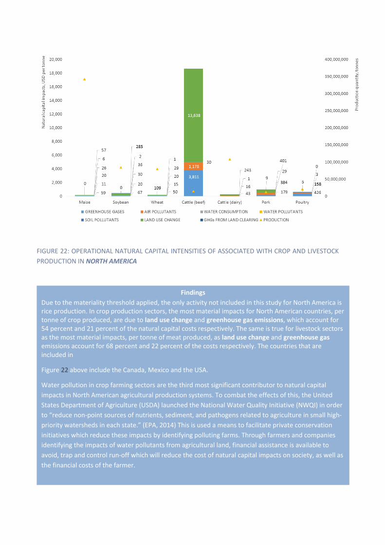
FIGURE 22: OPERATIONAL NATURAL CAPITAL INTENSITIES OF ASSOCIATED WITH CROP AND LIVESTOCK
PRODUCTION IN NORTH AMERICA
Findings
Due to the materiality threshold applied, the only activity not included in this study for North America is rice production. In crop production sectors, the most material impacts for North American countries, per tonne of crop produced, are due to land use change and greenhouse gas emissions, which account for 54 percent and 21 percent of the natural capital costs respectively. The same is true for livestock sectors as the most material impacts, per tonne of meat produced, as land use change and greenhouse gas emissions account for 68 percent and 22 percent of the costs respectively. The countries that are included in
Figure 22 above include the Canada, Mexico and the USA.
Water pollution in crop farming sectors are the third most significant contributor to natural capital
impacts in North American agricultural production systems. To combat the effects of this, the United
States Department of Agriculture (USDA) launched the National Water Quality Initiative (NWQI) in order
to “reduce non-point sources of nutrients, sediment, and pathogens related to agriculture in small high-
priority watersheds in each state.” (EPA, 2014) This is used a means to facilitate private conservation
initiatives which reduce these impacts by identifying polluting farms. Through farmers and companies
identifying the impacts of water pollutants from agricultural land, financial assistance is available to
avoid, trap and control run-off which will reduce the cost of natural capital impacts on society, as well as
the financial costs of the farmer.

FIGURE 23: OPERATIONAL NATURAL CAPITAL COSTS OF ASSOCIATED WITH CROP AND LIVESTOCK
PRODUCTION IN SOUTH AMERICA
Findings
Due to the materiality threshold applied, the activities that are not included in this study for South America are rice and wheat production. In crop production sectors, the most material impacts for South American countries, per tonne of crop produced, are due to land use change and water pollution, which account for 46 percent and 27 percent of the natural capital costs respectively. In livestock sectors in South America, the most material impacts, per tonne of meat produced, are land use change and greenhouse gases, which account for 83 percent and 14 percent of the costs respectively. The countries that are included in
Figure 23 above include the Argentina, Brazil and Uruguay. Please see
Table 6 and
Table 8 for a complete list of countries included in this analysis.
Beef production in Brazil emerged as having the highest costs of impacts on natural capital in the study.
Fertile land that provides valuable ecosystem services is converted in order to expand agricultural land.
The effects of land use change can be regional, in terms of the forest fragmentation, the loss of water
provisioning and soil erosion services, and the other is global, in terms of climate change. These impacts
have led to the emergence of mechanisms such as payments for ecosystem services (PES) as well as the
Reducing Emissions from Deforestation and Forest Degradation (REDD+) scheme. These initiatives can
provide opportunities for businesses to reduce its impact on the environment whilst ensuring its long-
term viability in operating in areas such as Brazil (Ometto et al, 2013).

51
PHASE 2: TRADE-OFFS OF DIFFERENT FARMING
SYSTEMS
The second phase of the study analyzed different farming practices that are used in the production of
four commodities. The analysis focused on the trade-offs that exist between adopting different farming
practices. The following trade-offs have been analyzed:
Cattle – conventional farming versus holistic grazing management in Brazil
Rice – conventional farming versus the system of rice intensification in India
Soybean – conventional farming versus organic farming in USA
Wheat – conventional farming versus organic farming in Germany
Each study is to serve as an example to businesses of how the impacts identified in the materiality
assessment in Phase 1 can be compared to more sustainable farming practices. The core objective of
the analysis is to demonstrate to agri-businesses that by measuring its impact, and indirectly its
dependency on natural capital, this can inform more sustainable farming decisions, increase
profitability, and ensure a more resilient and stable supply of each commodity.
Value Drivers
There are many reasons why businesses would seek to undertake an assessment of the impacts and
dependencies that exist within their operations and/or value chain. Specific value drivers that a
company might have for switching from conventional to more sustainable management practices
include mitigating risk, managing supply chains and strategically proofing its future activities. The typical
benefits that a company may derive include ensuring a longer term crop supply, diversifying revenue
streams, reducing input costs and maintaining its licence to operate.
Production costs
The following case studies include an overview of the change in revenues that farmers are likely to
expect as a result of switching to more sustainable farming practices. This is an important, and often
under-reported, aspect of switching to more sustainable farming systems.
A literature review was conducted and studies found that assesses the profitability of organic and non-
organic farming systems and finds that despite a drop in yield, the majority of cases show organic farms
to be more economically profitable, and yields are higher in cases of biophysical stress such as droughts
(Nemes, 2009). Pimentel et al. (2005) studied corn and soybean farming in the USA and indicates that
the total input costs for conventional farming is USD 354 per hectare, whereas for organic agriculture
the cost is around USD 281 per hectare, a 21 percent decrease, a result supported by Hanson et al.
(1997). In two studies comparing organic and conventional wheat production in Australia, input costs
were 40 percent and 74 percent lower than conventional farming practices (Wynen, 2001; Dumaresq,
2001). Similarly, rice farming in the Philippines revealed that the total operating costs of organic versus
non-organic farming systems decreased by 21 percent, despite a higher labour (13 percent) and seed
costs (35 percent) (Rubinos et al., 2007). Despite this, the study also showed that certain aspects of

organic farming had higher costs, such as seeding and machinery use, and the annual net return on
conventional farming was USD 184 per hectare and USD 176 per hectare for organic farming.
In the case of dairy farming, a study conducted in the USA calculated that the total input cost for organic
farmers in Minnesota was 23 percent less than for non-organic farmers. This was due to the fact that
organic herds have lower feeding costs than non-organic dairy cows as they rely on purchased
concentrate feed, protein, vitamins and minerals (Heins, 2011). Similarly, a study in Northern Ireland,
UK, shows that the decreasing availability of forage could mean that farmers have to pay between GBP
110 and GBP 140 per tonne (approximately USD 178 and USD 227) for concentrate feed for beef and
dairy cattle respectively (DARD, 2003).
Overview of Case Studies
A literature review assessed the benefits of the country-specific farming systems listed above. As the
studies used do not analyze all trade-offs from the two production systems, datapoints were combined
from a number of different studies. The studies that have been selected analyze the same production
practices as closely as possible, but in some instances the practices studied between studies do not
exactly mirror one another. As a result, specific practices vary slightly between the studies so there may
be some over- or underestimation of the natural capital impacts of alternative farming practices. To
analyze the impact of land use change for more sustainable farming systems, it was assumed that
farmers would want to maintain the same yields compared to conventional farming systems. Therefore,
if the alternative farming practice yields more tonnes per hectare, then the land use impact will
decrease, and vice versa.
The following case studies show that in the vast majority of cases, the cost of the natural capital impacts
of the more sustainable farming systems will decrease. They also show the benefits from switching to
these systems that cannot currently be monetized. For example, the benefits of increasing biodiversity
on and around farmland. Where data is available, there is also a discussion of the economic benefits
that farmers would achieve by farming more sustainably, which show in general, that gross margins and
operating costs for sustainable farming systems would increase with decreasing natural capital impacts.
53
CATTLE FARMING - BRAZIL
HOLISTIC GRAZING MANAGEMENT VS. CONVENTIONAL
Background
Overview
Conventional cattle farming relates to extensive grazing systems that predominate in Latin American
countries such as Brazil and Argentina (Deblitz and Ostrowski, 2004). The main production system of
beef in Brazil is extensive pastoralism; approximately 82% of beef cattle were raised under this system
in 2008 and the remainder were raised under feedlotting (Ferraz and de Felocio, 2010). Nevertheless, in
the past ten years production efficiency per hectare has improved by 25% (Brazilian Beef, n.d.).
Extensive cattle ranching is identified as the primary driver of deforestation in the Amazonian region,
and in Northern Brazil, cattle ranching has expanded at a rate of 9% per annum accounting for 70-80%
of total deforestation in the region over the period 1998-2008 (Kaimowitz et al, 2014; Nepstad et al,
2006).
Holistic grazing management involves mimicking grazing herds to reduce overgrazing and improve the
natural ecosystem that is being grazed (Savory Institute, 2013). Livestock are penned on sub-plots of
pasture to deposit manure, disturb land with their hooves, and feed on all available pasture as no feed
from external sources is required. Holistic grazing management involves grazing livestock in high
densities, on sectioned areas of pasture land called paddocks, which will be revisited by cattle after
specified regeneration periods have been observed. The pasture land is divided into small paddocks
which the livestock will graze over a standard period of time according to farming strategy. Although
holistic grazing management has widely reported benefits, such as improved biodiversity, there is a lack
of scientific evidence about herd impact on ecosystem responses, for example defoliation and recovery
of individual plants, due to greatly complicated inter-relationships between human management and
nature.
Brazil has been chosen as the case study country as it is one of the largest global producers of beef, and
is the largest contributor to global natural capital costs. These are largely due to the ecosystem services
lost due to land change use and the emissions from greenhouse gases (GHGs). Holistic grazing
management helps restore degraded pasture land and mitigates GHGs, and Brazilian cattle farming has
the greatest potential to mitigate its natural capital impact by switching farming practices, as almost all
of its impacts are due to land use change (87 percent) and greenhouse gas emissions (11 percent).
Managing natural capital in cattle farming
The beef industry is coming under increasing pressure to operate more sustainably, due to public
awareness of the high natural capital impacts. For example, one global company has committed to only
purchasing beef in Brazil from suppliers who are not associated with deforestation of the Amazon
(Cheeseman, 2015). Other value drivers that beef producers and agri-businesses might have for
switching from conventional cattle farming to holistic grazing management practices include; reducing
the potential impact of future regulations; better management of supply chains; reducing input costs
and; strategically future proofing its activities by ensuring a longer term feed supply from quality
pasture land (Savory Institute, 2013).

One of the key benefits of holistic grazing management is that it aids the restoration of the pasture land,
and in Brazilian cattle farming regions, farmers have experienced the degradation of pastures due to
overgrazing and selective grazing practices (Costa and Rehman, 1999). This leads to farmers needing to
fertilise land or expanding into frontier areas through deforestation to maintain productivity (de
Campos Bernardi et al., 2011; WWF, 2012). These practices increase natural capital costs whereas
holistic grazing management helps farmers better manage the land so that its existing natural capital
can be preserved (Teague et al., 2011).
Assigning a monetary valuation to ecosystem services helps to demonstrate the economic benefits of
maintaining good quality pasture land. The impact of losing these ecosystem services can be
internalized and transformed into financial costs when, for example, the use of fertilizers become
necessary, or the quality of the beef is compromised by a poorer diet from degraded pasture lands (de
Campos Bernardi et al., 2011). Calculating the cost of natural capital impacts helps farmers to evaluate
the potential risks they are exposing themselves to, the costs that they impose on society, and provide
an evidence base to change practices before those risks materially affect their profitability.
Methodology
Scope
Land use change and GHG emissions were assessed for both conventional farming and holistic grazing
management. Soil and water pollutants were not assessed in the baseline scenario so could not be
included in the case study, and no datapoints were found on the water consumption of holistic grazing
management. Table 11 below outlines the impacts that have been analyzed.
TABLE 11: SCOPE OF THE ASSESSMENT OF ORGANIC AND CONVENTIONAL CATTLE PRODUCTION
Category
Holistic
grazing
comparison
Reason for
change Explanation References
GHGs 18% less GHG
emissions
Pasture quality
improvement,
improved animal
health and
intensive grazing
management
An FAO study estimated the reduction in GHG
emissions for better pasture quality, animal
health and husbandry improvements, and
intensive grazing management in Brazil to be
18-29%. As this analysis focusses only on the
improvements from intensive grazing
management, the conservative estimate of
18% reduction is selected.
Gerber et al, 2013
Study conducted in
Brazil.
Land Use
Change USD 166 ha
-1
Natural ecosystem
of the pasture land
is maintained as
grassland.
Improvements in land management will lead to
the ecosystem changing from degraded
pasture land to grassland. The relative
improvement in ecosystem service value
compared to conventional cattle is USD 166
ha-1
.
Savory Institute, 2013
Study conducted in
various locations
globally.
Economic
Costs
USD 68 per
adult cow
Greater weight gain
of cows, improved
reproductive
success
Estimated benefit based on increased weight
gain from cows under rotational grazing
compared to continuous grazing of pastures.
Eaton et al, 2011 Study conducted in
Brazil.
Quantification and Valuation Approach

Table 12 provides an overview of the costs of the natural capital impacts by continuous grazing of
conventional cattle farming.
TABLE 12: NATURAL CAPITAL IMPACTS FROM BASELINE ANALYSIS
Category Impact Type
Natural capital costs
(USD per tonne of
production)
Natural
capital
impacts
GHGs 6 845
Land use change 52 440
The biophysical data underling these baseline monetary valuations were adjusted to reflect the benefits
that are derived from holistic grazing management. The operational GHG emissions for holistic grazing
management were calculated by applying the estimated reduction of 18 percent found by a previous
FAO study (Gerber et al, 2013), and adjusting the baseline figure accordingly. For land change use, the
baseline calculations were recalculated using the assumption that the quality of the land had improved
and provided a higher value of ecosystem services as opposed to the degraded pasture land. Further
detail can be found in Appendix XII.
Findings
Overview
Figure 24 compares the natural capital impacts of conventional grazing and holistic grazing
management. The reduction in natural capital impacts due to holistic grazing management in Brazil are
USD 6 838 per tonne of beef - a reduction of 11 percent.
FIGURE 24: MONETARY VALUE OF THE OPERATIONAL IMPACTS CAUSED BY PRODUCING ONE TONNE OF
BEEF IN BRAZIL

The natural capital impacts of restoring the pasture lands through better grazing management practices
results in a gain of ecosystem services that are valued at around USD 166 per hectare of land, or USD
5606 per tonne of beef produced. The improved ecosystem service value reflects the increasing quality
of the pasture land which includes important services such as climate regulation and erosion
prevention. GHG emissions were estimated to reduce by 18 percent for each tonne of beef produced,
resulting in a natural capital saving of USD 1 232 per tonne. These savings come about from better
pasture quality, improved animal health and husbandry and intensive grazing management, which will
provide additional benefits to the farmer that are not captured in this valuation.
The change in farming practices can also improve biodiversity on the pasture land and in surrounding
ecosystems. These potential benefits have not been valued in this study but are discussed qualitatively
in Section 3.3.
Economic costs
Limited data points were found on the economic costs and benefits of each farming practice. Of the
data that was found, the academic research was split on whether there are increased profits with
holistic grazing management or not. Some studies reported beneficial returns (Bryan et al., 1986;
Undersander et al., 2002) where others reported no difference (Bransby, 1991). However one study,
conducted in Mexico, did report greater net profit under holistic grazing management (Ferguson et al,
2013). Although these results were not statistically significant, improvements in livestock nutrition, soil
fertility, animal health and welfare were reported. Another study based in Brazil in 2009, stated that the
economic gain from holistic grazing management was approximately USD 68 per adult animal (Eaton et
al, 2011).
Other impacts
Biodiversity has not been directly valued in this case study, but is nonetheless an important factor to
successful cattle farming. In degraded soil, if holistic grazing management is followed for a span of three
years, insects that were previously forced out of the ecosystem, such as the dung beetle, return to the
ecosystem (Savory Institute, 2013). The fauna that return to restored ecosystems, such as moles and
prairie dogs, churn the soil and encourage deep rooted perennial grasses to regrow (Ibid). As a result of
a wider availability of higher quality grasses, plants are grazed more evenly and there is better
distribution of manure (Fears, 2013). Over time, the manure degrades into the soil and provides organic
matter which provides a better environment for microorganisms to flourish. This in turn, improves the
quality of the pasture and provides increasing amounts of grass for cattle to feed on, which reduces the
farmer’s reliance on purchased concentrate feeds (Eaton et al, 2011).
During grazing, cattle consume fresh plant material, which is rich in nitrogen and released back into soil
in the form of manure. When poorer quality grasses are not grazed, it dries and subsequently gets
oxidized by microorganisms which releases carbon dioxide into the atmosphere. The optimal carbon to
nitrogen ratio in the soil is 25-30:1 (Illinois University, 2015). As the carbon content of the soil increases,
organisms use more nitrogen to decompose the material and oxidise the carbon. The increased uptake
of nitrogen causes a reduction in soil fertility, which is combated by holistic grazing management as it
discourages the cattle from selectively grazing higher quality grasses only (Byck, 2013).
Finally, holistic grazing management delivers other benefits such as reducing incidents of livestock
morbidity, due to the absence of pesticides use, as well as the increasing diversity of flora on pasture
land that improves the dietary composition and health of cattle (Eaton et al., 2011; Fears, 2013).

Limitations
Owing to restrictions in data availability and the nature of holistic grazing management, the following
limitations were imposed on the analysis:
No direct data would be found on holistic grazing management studies in Brazil. This may be
due to the fact that it has various names in the literature including management-intensive
grazing, multiple-pasture grazing, short-duration grazing, cell grazing and controlled grazing
(Beetz and Rinehart, 2010).
No data could be sourced which detailed the impacts of water consumption by holistic grazing
management.
The impact on soil and water pollution were out of the scope of this study, meaning that any
potential costs or benefits provided by holistic grazing management could not be evaluated.
Conclusions
After analyzing available data sources, holistic grazing management shows a reduction in natural capital
impact compared to conventional cattle grazing. However, there are benefits outside the scope of this
study that cannot be monetized which include improving soil and plant biodiversity. The analysis shows
that natural capital impacts can be reduced by up to 12 percent by switching to holistic grazing
management practices, and this change is largely driven by the improvement in the quantity and quality
of ecosystem services. Due to a paucity of data points, the study was unable to quantify with much
certainty the economic benefits provided to the farmer by holistic grazing management practices.
Holistic grazing management is seen in some academic circles as controversial because of the extent
and scalability of its benefits (McWilliams, 2013). The rebuttal from Allan Savory points to the fact that
this is due to the holistic nature of the management practice, which requires the development of new
skills and training to implement successfully. He also cites that holistic grazing management is opposed
because it behaves contrary to the reductionist approach of academic research (Savory, 2013). As a
result, much of the evidence for its success is anecdotal (Byck, 2013) and not documented in peer-
reviewed journals.

RICE FARMING - INDIA
SYSTEM OF RICE INTENSIFICATION VS. CONVENTIONAL
Background
Overview
Conventional production in India refers to rice produced in paddies and involves the use of continuous
flooding (Kawasaki and Herath, 2011). Rice paddy production in India covered 42 million hectares and
produced nearly 158 million tonnes of rice in 2011 (FAOSTAT, 2014b). The system of rice intensification
(SRI) is a farming method developed in 1980s in Madagascar and is now used worldwide (De Laulanié,
2011). It increases rice yields through the better management of plants, soils, water and nutrients.
Some of the techniques involve:
Early, quick and healthy plant establishment.
Reduced planting density leading to less competition for soil nutrients.
Improved soil conditions through enrichment with organic matter.
The paddies are flooded intermittently, not continuously.
India is the second largest producer of rice after China, and despite this, it has greater natural capital
impacts from the on-site operations of its farming practices. Hence, India was selected as the case study
site, as its farmers and enterprises potentially have most to gain from changes to their management
practices.
Managing natural capital in rice farming
Specific value drivers that a farm might have for switching from conventional to SRI practices include
mitigating their exposure to water shortages through improved water efficiency, reducing input costs
through less pesticide use, and increasing profitability by improving rice yields (De Laulanié, 2011). The
typical benefits that a business may derive from switching to more sustainable agricultural practices
include ensuring longer term crop yields, minimising input costs and maintaining its licence to operate
(Palanshami et al., 2012; Jayapalreddy and Shenoy, 2013).
Water pollutants are a significant impact in the operational natural capital intensity of rice. Not only can
water pollutants directly impact the quality of water used for irrigation on the farm, and subsequently
affect the quality of the rice produced that may harm trade, but they can also affect downstream water
users, such as the health of the local labour force (Katakey and Chaudhary, 2013). Likewise, during
periods of drought, rice farmers could be affected by the availability of water, as governments may
restrict agricultural water use in favour of public water consumers, as was the case in Thailand in early
2015 (Jikkham and Wongyala, 2015). Assigning a natural capital cost to the impacts of water
consumption and water pollution from SRI and conventional farming practices helps to demonstrate the
risks and mitigation potential of switching to more sustainable farming practices.
One of the key benefits of SRI is its diminished use of water. Traditional rice practices involve the
continuous flooding of paddies and thus yields can be affected severely during times of drought
(Kawasaki and Herath, 2011). Flooded rice fields are also significant sources of methane emissions and
paddy rice generates approximately 500 million tonnes of carbon dioxide equivalent (CO2e) annually

(WRI, 2014). Finally, SRI increases yields whilst using less input and thus are expected to create a more
profitable farming practice that is both resilient to external pressures and places less dependence on
natural capital (Chowdhury et al., 2014). For example, SRI can reduce pesticide expenditures by 96
percent, from 49 to 2 USD per hectare, reducing the natural capital impacts of soil pollution whilst
maintaining adequate pest control (Jayapalreddy and Shenoy, 2013). Using SRI methods, fertilizer spend
can also be reduced in instances by up to a third, which subsequently reduces the impacts of water
pollution (Rajendran et al., 2007).
Methodology
Scope
Greenhouse gas (GHG) emissions, water pollutants, water consumption, air pollutants, soil pollutants,
land use change and economic costs were assessed for both conventional and SRI practices. Table 13
below outlines impacts that have been analyzed. All information relates to operational impacts of rice
farming in India.
TABLE 13: SCOPE OF THE ASSESSMENT OF SRI AND CONVENTIONAL RICE PRODUCTION
Category SRI comparison Reason for
change Explanation References
GHGs
23% (combined)
less methane and
nitrous oxide
emissions
Attributed to
planting, water
and fertilizer
management
practices
Fluctuations in methane and nitrous
oxide emissions due to intermittent
drying and wetting.
(Jain et al., 2014)
Study conducted in India.
Air Pollutants 72% less
ammonia
emissions
Reduced fertilizer
expenditure
Assumed linear relationship between
reduced fertilizer spend in SRI and
ammonia emissions.
(Zhao et al, 2010a)
Study conducted in China
(Rajendran et al, 2007)
Study conducted in India.
Water
Consumption
64% less water
usage
Fields are flooded
intermittently and
not continuously
Reduced water consumption due to
changes in irrigation practices.
(Chowdhury et al, 2014)
Study conducted in India.
Water
Pollutants
2.9% and 4.5%
reduction in
nitrogen and
phosphorus load
Fields are flooded
intermittently and
not continuously
Total nitrogen and total phosphorus
loads reduced after applying
recommended ponding depth
management practices.
(Jung et al, 2014)
Study conducted in South
Korea.
Soil Pollutants 2.9% reduction
Reduced
pesticides
expenditure
Assumed linear relationship between
reduced pesticides spend in SRI and
soil pollutants.
(Jayapalreddy and
Shenoy, 2013)
Study conducted in India.
Land Use
Change
26% reduction in
land use
To maintain
conventional
yields, less land is
required
Rice yields are found to be higher
India-wide for SRI rice farms
(Palanshami et al., 2012)
Study conducted in India.
Economic 18% increase in
gross margin per
hectare
Higher yields and
lower operating
costs in SRI
practices
SRI uses less inputs, has lower
operating costs, has higher yields,
and thus is a more profitable farming
system.
(Palanshami et al., 2012)
Study conducted in India
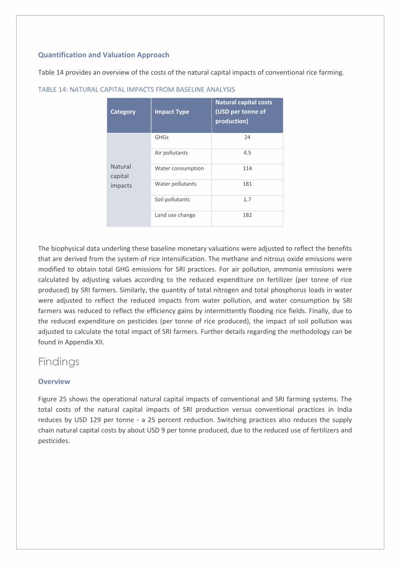
Quantification and Valuation Approach
Table 14 provides an overview of the costs of the natural capital impacts of conventional rice farming.
TABLE 14: NATURAL CAPITAL IMPACTS FROM BASELINE ANALYSIS
Category Impact Type
Natural capital costs
(USD per tonne of
production)
Natural
capital
impacts
GHGs 24
Air pollutants 4.5
Water consumption 114
Water pollutants 181
Soil pollutants 1.7
Land use change 182
The biophysical data underling these baseline monetary valuations were adjusted to reflect the benefits
that are derived from the system of rice intensification. The methane and nitrous oxide emissions were
modified to obtain total GHG emissions for SRI practices. For air pollution, ammonia emissions were
calculated by adjusting values according to the reduced expenditure on fertilizer (per tonne of rice
produced) by SRI farmers. Similarly, the quantity of total nitrogen and total phosphorus loads in water
were adjusted to reflect the reduced impacts from water pollution, and water consumption by SRI
farmers was reduced to reflect the efficiency gains by intermittently flooding rice fields. Finally, due to
the reduced expenditure on pesticides (per tonne of rice produced), the impact of soil pollution was
adjusted to calculate the total impact of SRI farmers. Further details regarding the methodology can be
found in Appendix XII.
Findings
Overview
Figure 25 shows the operational natural capital impacts of conventional and SRI farming systems. The
total costs of the natural capital impacts of SRI production versus conventional practices in India
reduces by USD 129 per tonne - a 25 percent reduction. Switching practices also reduces the supply
chain natural capital costs by about USD 9 per tonne produced, due to the reduced use of fertilizers and
pesticides.

FIGURE 25: MONETARY VALUE OF THE OPERATIONAL IMPACTS CAUSED BY PRODUCING ONE TONNE OF
RICE IN INDIA
The largest contributors to the reduction in the cost of the natural capital impacts in SRI practices are
land use change, water consumption and water pollution. The cost of each of these natural capital
impacts in SRI practices reduced by USD 48 (26 percent), USD 41 (36 percent), and USD 29 (16 percent)
per tonne of rice produced. SRI practices also significantly reduce the costs of soil pollution and air
pollution as each of these impacts decrease by 97 percent and 78 percent respectively.
There are additional benefits outside the scope of this project that could increase the value delivered by
SRI farming practices, such as improving biodiversity. These benefits have been discussed qualitatively
in Section 3.3.
Economic analysis
A survey, based on 2011 data from 2 234 SRI and conventional farms across India, reported yields of
3.79 tonnes per hectare for conventional and 4.64 tonnes per hectare for SRI (Palanshami et al., 2012).
Prices varied slightly, and rice produced via the SRI method fetched a price 38 percent higher than
conventional practices (USD 74 per tonne for conventional and USD 103 for SRI).15 The gross margin for
SRI farmers was USD 190 per tonne, whereas conventional rice in India had a gross margin of USD 196
per tonne in the same growing season - a 3 percent decrease. Gross margins were 18 percent higher per
hectare for SRI farmers whereas operating costs were 13 percent lower. However, when comparing the
operating costs per tonne of rice production, the cost reduction for SRI farmers compared to
conventional production was 29 percent.
15 Prices were reported in Rupees and have been adjusted for inflation and converted to 2013 USD.

Other impacts
Increasing biodiversity on rice fields helps to maintain soil fertility and reduce pests without the use of
artificial pesticides (Zhao et al., 2010b; Way and Heong, 1994). Soil biota are the key drivers of fertility
and a strong relationship exists between soil biodiversity and its productivity. Thiyagarajan and Gujja
(2013) demonstrated that SRI plants had higher uptake of nitrogen, which suggests greater activity of
nitrogen fixing bacteria, which could explain the reduction in water pollution from SRI practices.
Furthermore, increasing concentrations of biota, such as earthworms, aided an increase in water
infiltration, whereas other organisms such as termites and ants form an important part of soil food web
which helps to store and release soil nutrients (Thiyagarajan and Gujja, 2013).
Limitations
No data could be found specific to water pollution in India, hence a study based in South Korea
was used. The reduction of water pollutants was also assumed to be linear because of limited
data availability, which might not be the case. Until a greater number of quantitative and
qualitative data points studying this effect have been published, it is not possible to test this
hypothesis.
No data could be found specific to ammonia emissions from fertilizer application under SRI and
conventional rice farming in India, hence a study based in China was used. However,
information on the reduced fertilizer spend was taken from a study in India.
A linear relationship between pesticide use and soil pollution was assumed because of limited
data availability, which might not be the case. Until a greater number of quantitative and
qualitative data points studying this effect have been published, it is not possible to test this
hypothesis.
Conclusions
The system of rice intensification offers clear environmental benefits compared to conventionally
flooded rice farming systems in India. The analysis shows that the cost of natural capital impacts can be
reduced by 25 percent largely due to the reduced impacts of land use change, water consumption and
water pollution. There is also a case for switching farming practices based on economic performance of
SRI systems. The increase in yields and decrease in input costs allowed the gross margin per hectare to
increase by 18 percent for SRI. It is important to note that these results will vary across locations in
India, and that the impacts could increase or decrease based on specific local environmental conditions.
The analysis shows that the system of rice intensification, at a national level, offers an opportunity to
reduce the environmental impacts of rice production whilst increasing income for local farmers.

SOYBEAN FARMING - UNITED STATES OF AMERICA
ORGANIC VS. CONVENTIONAL
Background
Overview
Conventional soybean farming has evolved to incorporate crop rotations whereas organic practices
have gone a step further and avoid the use of synthetic inputs. Organic soybean farming has also
evolved over the years to incorporate the use of cover crops, organic fertilizers, the implementation of
best management practices of soils, as well as the elimination of pesticides (Pimentel, 2005). In this case
study, farming that incorporates the use of these practices is referred to as organic farming systems.
This study shows that the USA is the largest producer of soybeans, ahead of Brazil and Argentina, in
second and third place respectively, and the annual natural capital costs of its soybean production are
37 percent higher than the total revenue that the sector generates each year. To combat these impacts,
the USA has started to collect data on its sustainable practices over the last few decades. For instance,
the Soybean Sustainability Assurance Protocol (SSAP) is reporting an estimated 47 percent reduction of
greenhouse gases (GHGs), 65 percent decrease in soil erosion, and 46 percent less energy used per
tonne of soybean produced since 1980 on their certified farms (SSAP, 2013). As a result, the USA was
selected as the country for this case study.
Managing natural capital in soybean farming
Specific value drivers that a farm might have for switching from conventional to organic practices
include mitigating the impacts of climate change, reducing the natural capital impacts on the farm, and
strategically future proofing its activities. The typical benefits that a business may derive from switching
to more sustainable agricultural practices include ensuring longer term crop yields, minimizing input
costs, and ensuring long-term demand from its farm (Pimentel, 2005; Delate et al., 2003).
A 22 year-long study comparing organic legume-based, and organic animal-based farming, incorporating
corn crop rotations, and conventional soybean farming, based on synthetic fertilizer and herbicide use
as well as a simple five year crop rotation, found there to be similar yields (Pimentel, 2005), whereas
other studies estimate organic yields at 92 percent of conventional farms (de Ponti et al., 2012). In the
study by Pimentel (2005), the annual net return for the conventional system was USD 184 per hectare
versus USD 176 for the organic legume-based system. When the costs of the biological transition for the
organics system was considered, over a three year period, net returns reduced to USD 162 per hectare.
The organic farms had more consistent financial results year-on-year, as the standard deviation for net
returns over a ten year period were USD 127 for the conventional system versus USD 109 for the
organic rotation. This suggests that conventional farming practices are more likely to be affected by
environmental stress such as droughts and increases in pest populations.
One of the key benefits of organic soybean farming is the reduced input costs that are achieved by
eliminating pesticide use in addition to the price premium received for organic produce. For example,
one study predicts that the profit per hectare is 368 percent higher than conventional soybean (Delate
et al., 2003). The elimination of pesticide use also avoids soil pollution, and promotes natural pest
regulation, an ecosystem service that reduces the dependency of farmers on synthetic inputs.

Around 85 percent of the world’s soybean crop is processed into meal and vegetable oil, and almost all
of that oil is used as animal feed (Soyatech, 2015). Soybeans are an important source of feed for pork
production, but can also be used for biofuels and for human consumption (NCSPA, 2014; WWF, 2012).
There are significant natural capital impacts in livestock supply chains and, as pressure mounts for
livestock farmers to reduce their natural capital impact, this pressure could also be felt financially by
soybean farmers (Opio et al., 2013).
Methodology
Scope
Greenhouse gas (GHG) emissions, air pollutants, water consumption, water pollutants, soil pollutants
and economic costs were assessed for both conventional and organic soybean farming. Land use change
was not compared as it was assumed that yields between organic and conventional farming remain
relatively equal, so an expansion of land to maintain production is not required (Pimentel, 2006). Table
15 below outlines impacts that have been analyzed.
TABLE 15: SCOPE OF THE ASSESSMENT OF SUSTAINABLE AND CONVENTIONAL SOYBEAN PRODUCTION
Category
Organic
soybean
comparison
Reason for change Explanation References
GHGs 12% reduction Change in
management practices
Energy reduction due to a change
in management practices. Data
taken from LCA database Ecoinvent
v2.2.
(Meier, 2015)
Global study.
Air Pollution 88% reduction
in ammonia
emissions
Use of organic fertilizer
Use of slurry and manure instead
of synthetic fertilizers emits less
ammonia emissions to the air.
Based on LCA modelling
(Meier et al., 2014)
Global study.
Water
Consumption 54% reduction
Change in
management practice
Water reduction due to a change in
management practices. Data taken
from LCA database Ecoinvent v2.2.
(Meier, 2015)
Global study.
Water
Pollution
36% reduction
in phosphorus
use; zero
nitrogen use
Changes in fertilizer
practices
Organic practices do not need to
add nitrogen-based fertilizers and
use less phosphorus-based
fertilizers. Assumed that this
directly results in less leaching.
(Pimentel, 2006)
Study conducted in the
USA.
Soil Pollution Zero pesticide
use
No synthetic pesticides
applied
Pesticides are used in conventional
but not organic farming practices.
(Pimentel, 2006)
Study conducted in the
USA.
Economic 220% increase
in gross margin
per tonne
Price premium and
lower operating costs
per hectare for organic
Organic soybean attain a higher
market price that is 167% higher
than conventional soybeans.
(McBride and Green,
2009) Study conducted in
the USA.
Quantification and Valuation Approach

Table 16 provides an overview of the costs of the natural capital impacts of conventional soybean
farming.
TABLE 16: NATURAL CAPITAL IMPACTS FROM BASELINE ANALYSIS
Category Impact Type
Natural capital costs
(USD per tonne of
production)
Natural
capital
impacts
GHGs 67
Air pollutants 20
Water consumption 30
Water pollutants 36
Soil pollutants 1.7
The biophysical data underling these baseline valuations was adjusted to reflect the benefits that are
derived from organic soybean farming. The GHG reduction, described in Table 15 was used to calculate
the new GHG emissions and to calculate the impacts of air pollution, the ammonia emissions were
adjusted by the yield to give an emissions factor for ammonia in kilogrammes per tonne of soybean.
Similarly, the quantity of total phosphorus leaching was adjusted to reflect the reduced phosphorus use,
and the total impacts from nitrogen leaching were removed. Finally, due to the lack of pesticides used in
organic soybean, the impact of soil pollution was assumed to be zero. Further detail regarding the
methodology can be found in Appendix XII.
Findings
Overview
The total natural capital impact savings from organic soybean production in the USA is USD 72 per tonne
- a 16 percent reduction. Figure 26 shows the overall results from the natural capital impacts of
conventional and organic farming systems.

FIGURE 26: MONETARY VALUE OF THE OPERATIONAL IMPACTS CAUSED BY PRODUCING ONE TONNE OF
SOYBEAN IN THE UNITED STATES OF AMERICA
The use of sustainable practices reduces the natural capital impacts of water pollution by USD 27, air
pollution by USD 19, and water consumption by USD 16 per tonne of soybeans. The cost of the natural
capital impacts of soil pollution, while not as significant, reduced by USD 1.7 per tonne, or 100 percent.
The impact of GHG emissions decreased by USD 8 per tonne, approximately 12 percent. The total
natural capital impacts that are avoided due to organic soybean farming are USD 72 per tonne, a
reduction of 16 percent.
There are ecosystem services outside the scope of this project that could increase the difference in the
value delivered by conventional and organic systems, such as improving biodiversity. However, these
benefits have been included qualitatively in Section 3.3.
Economic analysis
A survey, based on 2006 data from 237 organic farms and 1 425 conventional farms, reported yields of
3.16 tonnes per hectare for conventional and 2.09 tonnes per hectare for organic farming – a 34
percent decrease (McBride and Green, 2009). Organic soybean fetched a price of USD 622 per tonne, a
167 percent increase over conventional which fetched USD 233.16 The gross margin for organic
soybeans was USD 481 per tonne, whereas conventional soybean in the USA had a gross margin of USD
150 per tonne in the same growing season (a 220 percent increase). Operating costs for organic
soybeans were 70 percent higher per tonne, or 12 percent higher per hectare due to the decrease in
yield, however the price premium for organic soybeans increased its overall returns.
Yields of organic soybeans have improved in more recent times, which has been demonstrated by a
meta-analysis study that shows yields in the USA were on average only 8 percent lower than
conventional farming systems (de Ponti et al, 2012). If the 2006 yields from the McBride and Green
study had been comparable to current trends, operating costs per tonne of soybeans would have been
16 Prices were reported in 2006 USD and have been adjusted for inflation so now represent 2013 USD.

22 percent higher for organic systems, a 48 percent decrease from the previous value calculated from
McBride and Green. The operating costs for organic systems would have been USD 101 per tonne
versus USD 83 for conventional farms, making organic farms even more profitable as gross margins
would increase to USD 622 per tonne.
Other impacts
After harvest and before the next planting of annual cash crops like soy, cover crops can be planted in
the same field to provide additional benefits to farmers (Pimentel, 2005). Cover crops are planted for
their benefits to soil, such as erosion prevention, which can subsequently be harvested for sale or used
to increase organic matter in the soil (SARE, 2012). The use of cover crops can also increase plant
diversity around the farm over a number of years (Larsen, 2013).
Cover crops trap residual nitrogen and prevent it from leaching to water sources and can also protect
the soil from getting eroded due to wind and rain (Corn Soybean Digest, 2014). In Iowa, rye cover crops
are used in no-tillage soybean production, which reduced inter-rill erosion by 54 percent and rill erosion
by 90 percent when compared to no-tillage without cover crops (Singer, 1999). The residue left over
from cover crops gets decomposed in the soil and provides organic matter for building soil structure,
which enriches the biota (SARE, 2012). Finally, cover crops aid water infiltration and nutrient recycling
through the deposition of phosphorous, the trapping of nitrates and sequestration of carbon,
encourages the improvement of biodiversity which reduces the need for pesticide use, which all provide
benefits directly or indirectly to the farmer (Salon, 2012).
Organic farms tend to grow a wider range of crops per farm than conventional farms (de Ponti et al
2012). Under organic practices, the soil exhibits undisturbed decomposition of humus and provides
habitat for active biotic community (Mäder et al, 2002). For example, the colonisation of root length by
mycorrhizae fungi was 2.5-10 times greater on low-input organic soybean farming, which is important
for the natural transfer of nutrients from the soil to the plants (Douds et al, 1993; Royal Horticultural
Society, 2015). Mycorrhizae fungi have added benefits as they also sequester carbon, encourage
biodiversity and ecosystem restoration, maintain long term soil fertility, and can even reduce drought
stress in soybean (Wilson et al., 2009; Leake et al, 2004; Jefferies et al, 2003; Bethlenfalvay et al, 1988).
The production of genetically modified (GM) soybeans create unique, and until now, mostly
unquantifiable impacts on biodiversity. Soybean is currently harvested on over 110 million hectares of
land globally and nearly 80% of this is due to the production of GM soybean (FAOSTAT, 2014b; GMO
Compass, 2014). GM crops can impact ecosystem service provision (Lovei, 2001), farm biodiversity
(Firbank, 2003), weed abundance and diversity (Heard et al., 2003), and the development of toxin
resistant insect strains (Cerda and Wright, 2002; Garcia and Altieri, 2005). These impacts are currently
not captured in monetary valuations conducted in this study, but should carry considerable weight
when assessing the costs of benefits of GM farming practices.
Limitations
The decline of water pollution due to the reduction in phosphorus use was assumed to be linear
because there of limited data availability. Until a greater number of quantitative and qualitative
data points studying this effect have been published, it is not possible to test this hypothesis.

A very limited amount of data on the blue water consumption in organic soybean farming could
be found, so a general percentage reduction in water use had to be applied. Water use in
conventional soybean farming relates to blue water use only.
It was assumed that because no nitrogen-based fertilizers are used in organic farming, there
would be no nitrogen leaching that contributed towards water pollution.
Not all studies used to calculate the different natural capital impacts of organic soybean farming
analyze the same management practices.
Conclusions
Organic soybean farming has both economic and natural capital advantages over conventional soybean
farming in the USA. The analysis shows that natural capital impacts can be reduced by 16 percent largely
due to the reduction in water pollution, air pollution and water consumption. The reduction of the
natural capital impacts from these three categories result in savings of, respectively, USD 27, USD 19
and USD 16 per tonne of soybean production. The gross margin for organic soybean can be increased by
up to 220 percent, which can mainly be attributed to the price premium paid for organic produce.
Finally, organic soybean farming delivers additional benefits such as improving soil structure, water
filtration and reduced soil erosion, which helps to maintain long-term yields and farm profitability.

WHEAT FARMING - GERMANY
ORGANIC VS. CONVENTIONAL
Background
Overview
Conventional wheat farming involves the application of synthetic fertilizers and pesticides whereas
organic wheat farming practices have evolved to include the use crop rotation, cover crops, organic
fertilizers, elimination of pesticides, changing irrigation practices and the deployment of new soil
management practices (McCoy, 2005).
Germany, ranked 9th in terms of total wheat production compared to China and India, respectively the
two largest producers of wheat, generates a disproportionately high impact on natural capital, the
majority of which are realised in its operations. The operational impacts of Germany’s wheat production
on natural capital are only 8 percent lower than those found in China despite the latter producing over 5
times more wheat. For these reasons, Germany was selected as the case study location, as small
changes in farm practices can significantly reduce the cost of natural capital impacts.
Organic agriculture can minimise the impacts caused by pesticide and fertilizer application in
conventional wheat farming, but it is widely argued that the removal of fertilizers and pesticides
negatively affects yields (Biello, 2012). More than external inputs, it is rotations and associations that
build-up fertility in organic systems, so the timeframe is crucial in comparing outcomes. Studies have
found that yields of organic wheat can equal conventionally farmed wheat and this case study aims to
assess the environmental impacts and yields of both of these practices (Ponisio et al., 2014).
Managing natural capital in wheat farming
Specific value drivers that an enterprise might have for switching from conventional to organic practices
include mitigating the impacts of climate change and reducing the potential impact from droughts. The
typical benefits that a company may derive from switching to more sustainable agricultural practices
include protecting and maintaining yields against environmental pressures such as droughts, minimising
input costs, diversifying revenue streams (through crop rotation), and maintaining its licence to operate
(Al-Karaki et al., 2004; Nieberg and Rahmann, 2005).
In Germany, farmers have the greatest exceedance of critical nutrient loads (EEA, 2014), which means
that nitrogen is emitted beyond EU ‘safe’ limits, which is a major explanatory factor why water pollution
represents 95 percent of wheat’s operational natural capital impacts. Water pollution has a direct
impact on the water treatment costs of a watershed, can directly impact land and property prices thus,
devaluing the asset of the farmland itself, and can have a negative impact on human health (McDonald
and Shemie, 2014; Dodds et al., 2009; Townsend et al., 2003; WHO, 2002).
One of the key benefits of organic wheat farming is that it helps to preserve soil nutrients by reducing
fertilizer use and by using nitrogen-fixing cover crops, which studies have shown can increase crop
yields (Kumar and Goh, 2002). Therefore organic farming can significantly reduce nitrate leaching, which
provides cleaner water and reduces the negative impact on ecosystems caused by eutrophication
(Hörtenhuber et al., 2014).

Methodology
Scope
Greenhouse gas (GHG) emissions, air pollutants, water pollutants, soil pollutants, land use change, and
economic costs were assessed for both conventional and organic wheat farming.
Table 17 below outlines the impacts that have been analyzed. All information relates to of the
operational impacts of wheat farming in Germany.
TABLE 17: SCOPE OF THE ASSESSMENT OF ORGANIC WHEAT PRODUCTION
Category Organic wheat
comparison Reason for change Explanation References
GHGs 73% reduction in
GHG emissions
Converting to organic
fertilizer
Reduction is attributed to reduced
emissions from changes in synthetic
fertilizer use, crop rotation and
reduced waterlogging during heavy
rain (which releases N2O).
An LCA study
(Hirschfeld et al., 2008)
Study conducted in
Germany.
Air
Pollutants
65% reduction in
ammonia
emissions
Converting to organic
fertilizer
Emissions from slurry and solid
manure based on figures from 2011.
An LCA study
(Meier et al, 2014)
Study conducted in
Switzerland.
Water
Pollutants
38% reduction in
nitrate leaching
Converting to organic
fertilizer
Reduction in nitrate leaching into
local water bodies from wheat
producers.
(Hörtenhuber et al.,
2014)
Study conducted in
Austria.
Soil
Pollutants Zero pesticide use
No synthetic pesticides
used
Elimination of pesticides and
introduction of natural predators
(Weber et al., 2002)
Study conducted in
Germany.
Land Use
Change
27% yield
reduction
Converting to organic
fertilizer; No synthetic
pesticides used
Organic wheat has slightly reduced
yields compared to conventional
farming practices
(de Ponti et al, 2012)
Economic 315% increase in
gross margin
Price premium and
lower operating costs
per hectare for organic
Organic wheat fetches higher
market prices and achieves lower
operating costs due to reduced
fertilizer and pesticide use.
(Nieberg and Rahmann,
2005) for organic;
(European Commission,
2013) for conventional

Quantification and Valuation Approach
Table 18 provides an overview of the costs of the natural capital impacts of conventional wheat farming.
TABLE 18: NATURAL CAPITAL IMPACTS FROM BASELINE ANALYSIS
Category Impact Type
Natural capital costs
(USD per tonne of
production)
Natural
capital
impacts
GHGs 59
Air pollutants 18
Water pollutants 2 396
Soil pollutants 2.5
Land use change 56
The biophysical data underling the baseline monetary valuations was adjusted to reflect the benefits
that are derived from organic wheat farming. The operational GHG emissions for organic wheat farming
were calculated in an LCA by Hirschfeld et al. (2008) and used to replace baseline factors. For air
pollution, ammonia emissions from Meier et al. (2014) were adjusted by the change in wheat yields to
give ammonia emissions in kilogrammes per tonne of wheat. Similarly, the impact of water pollution
was calculated by adjusting the amount of nitrate leaching that was coming from organic fertilizer.
Finally, as no pesticides are used in organic wheat production in this case study, the natural capital
impact associated with soil pollution is zero. Further details regarding the methodology can be found in
Appendix XII.
Findings
Overview
The reduction in natural capital impacts due to organic wheat farming in Germany are approximately
USD 1 166 per tonne - a 46 percent reduction. Figure 27 compares the natural capital impacts of
conventional and organic wheat farming systems.

FIGURE 27: MONETARY VALUE OF THE OPERATIONAL IMPACTS CAUSED BY PRODUCING ONE TONNE OF
WHEAT IN GERMANY
The impact of using organic fertilizers reduces the natural capital cost of water pollution by USD 1 122
per tonne of wheat produced, a 47 percent reduction. GHG emissions were estimated to be reduced by
73 percent per tonne of wheat produced, resulting in the costs of natural capital impacts reducing by
USD 43 per tonne. The impacts associated with land use change increase by 23 percent, or USD 13 per
tonne, as more land is required to maintain total production volumes resulting from organic yield
reductions.
There are ecosystem services outside the scope of this project that could increase the difference in the
value delivered by organic systems, such improving biodiversity. However, these benefits have been
included qualitatively in Section 3.3 below.
Economic analysis
A survey, based on 217 organic farms in Germany highlights the motivations for moving away from
conventional farming practices, which are broken down into environmental (38 percent), economic (29
percent) and political considerations (20 percent) (Nieberg and Rahmann, 2005). The study shows there
has been an increase in economically-driven switches, with only 15 percent of organic farmers thinking
about reconverting to conventional farming. In this survey, farmers reportedly had yields of 3.5 tonnes
per hectare with an average price of USD 509 per tonne. The gross margin was USD 478 per tonne,
whereas conventional wheat in Germany had a gross margin of USD 115 per tonne in the same growing
season (European Commission, 2013).17 Operating costs were 34 percent higher per tonne of organic
wheat due to the decrease in yield, whereas they were 32 percent lower per hectare compared to
conventional farms. The revenue generated by organic farms was 157 percent greater per tonne of
wheat than for conventional farms.
17 Figures were reported in 2002 Euros and have been adjusted to 2013 USD. The wheat in this study refers exclusively to the growing of winter wheat.
However, yields have improved in organic farming as demonstrated by a meta-analysis study by de
Ponti et al. (2012). If the yields from the 2002 study had been comparable to current trends, operating
cost would have been 7 percent lower per tonne of wheat produced, making it even more profitable.
Another factor in the profitability of organic wheat farmers is the price premium which is received for
organic produce. In 2002, the price for conventional wheat in Germany averaged at USD 176 per tonne
(European Commission, 2013), and even if the price premium of organic wheat was removed so that it
equalled the national average, then the gross margin per tonne of organic wheat would drop to USD
145 per tonne, which is still higher than the gross margin for conventional farmers (USD 115 per tonne).
Other impacts
Organic wheat farming has other impacts that are not captured in the above valuation. For example,
through organic farming, it is possible to re-introduce traditional crop varieties that better adapt to local
climatic conditions and promote agricultural biodiversity (FAO, 2003). A study on wheat in Germany
illustrates that, where sandy soils are common, soil nitrogen gets easily washed away due to spring rain.
This impact was tackled by using a native variety of wheat, which has a vegetative cycle that fixates
more of the available nitrogen in the soil (Ibid), therefore limiting the natural capital impacts of water
pollution which affects human health and ecosystems (WHO, 2002; WHO, 1999).
Organic farms tend to grow a wider range of crops per farm than conventional farms (de Ponti et al.,
2012). Under organic practices, the soil exhibits undisturbed decomposition of humus and provides
habitat for an active biotic community (Mäder et al., 2002). For example, the colonisation of root length
by mycorrhizae fungi was 40 percent higher on organic farming (Ibid). This is important for the natural
transfer of nutrients from the soil to the plants, which synthetic fertilizers replace (Royal Horticultural
Society, 2015). Mycorrhizae fungi have added benefits as they also sequester carbon, encourage
biodiversity and ecosystem restoration, maintain long term soil fertility, and can even reduce drought
stress in soybean (Wilson et al., 2009; Leake et al, 2004; Jefferies et al, 2003; Bethlenfalvay et al, 1988).
Finally, mycorrhizae fungi can even reduce drought stress in wheat (Al-Karaki et al, 2004).
Limitations
Studies have been collected from peer-reviewed and, where possible, papers that have
conducted meta-analyses. However, there are limited numbers of such studies to draw from.
For two of the impacts, air and water pollution, data could not be found for Germany
specifically. Instead, data was used from studies conducted in Switzerland and Austria.
The economic analysis was taken from two different sources and hence there may have been
discrepancies in types of costs included.
Not all studies used to calculate the different natural capital impacts of organic wheat farming
compared to conventional practices analyze the exact same management practices between
studies.

Conclusions
Organic wheat farming has both economic and natural capital advantages over conventional wheat
farming in Germany. The analysis shows that the cost of natural capital impacts can be reduced by 46
percent largely due to the reduction in water pollutants. There are also reductions in the emission of
GHGs, air, land and water pollutants. However, the impacts from land use change would be expected to
increase as more land would be required to maintain yields. The impacts from water consumption are
assumed to be the same across both farming practices. This is because only groundwater is included in
the scope of this analysis and wheat production in Germany is predominantly irrigated with rainwater.
The gross margin for organic wheat can be increased by 315 percent, due to the price premium and
reduced operating costs when compared with conventional.

75
REFERENCES
Agroecology. (2015) Agroecology. [Online] Available from: http://www.agroecology.org/ [Accessed:
10.02.15]
Al-Karaki, G., McMichael, B., Zak, J. (2004) Field response of wheat to arbuscular mycorrhizal fungi and
drought stress. Mycorrhiza, 14(4), pp. 263-269.
Altieri, M. A., Nicholls, C. I. (2005) Agroecology and the Search for a Truly Sustainable Agriculture. United
Nations Environment Programme. ISBN: 968-7913-35-5
Bethlenfalvay, G. J., Brown, M. S., Ames, R. N., Thomas, R. S. (1988) Effects of drought on host and endophyte
development in mycorrhizal soybeans in relation to water use and phosphate uptake. Physiologia
Plantarum, 72(3), pp. 565-571.
Beetz, A. E., Rinehart, L. (2010) Rotational Grazing. [Online] Available from: www.attra.ncat.org/attra-
pub/rotgraze.html [Accessed on: 09.03.15]
Biello, D. (2012) Will Organic Food Fail to Feed the World? Scientific American. [Online] Available from:
http://www.scientificamerican.com/article/organic-farming-yields-and-feeding-the-world-under-
climate-change/ [Accessed on: 23.03.15]
Blonk Consultants. (2014) The Direct Land Use Change Assessment Tool [Online] Available from:
http://blonkconsultants.nl/en/tools/land-use-change-tool.html [Accessed on: 11.11.14]
Brander, L. (2013) Guidance Manual on Value Transfer Methods for Ecosystem Services. United Nations
Environment Programme (UNEP)
Bransby, D. I. (1991) Biological Implications of Rotational and Continuous Grazing: A Case for Continuous
Grazing. Forage and Grassland Conference. American Forage and Grassland Council.
Brazilian Beef. (n.d.) The Beef Sector: Brazilian Livestock. [Online] Available from:
http://www.brazilianbeef.org.br/texto.asp?id=18 [Accessed on: 11.06.15]
Brumfield, R. G., Rimal, A., Reiners, S. (2000) Comparative Cost Analyses of Conventional, Integrated Crop
Management, and Organic Methods. The State University of New Jersey. Department of Agriculture,
Food, and Resource Economics.
Bryan, W. B., Prigge, E. C., Burton, R. O. (1986) Beef Cow/Calf Production on Conventional and Innovative
Systems. Forage and Grassland Conference. American Forage and Grassland Council.
Byck, P. (2013) Soil Carbon Cowboys. [Online Video]. 27 November. Available from:
https://vimeo.com/80518559. [Accessed on: 17.03.15]

76
Cerda, H., Wright, D. J. (2002) Could resistance to transgenic plants produce species of insect pest?
Agriculture, Ecosystem and Environment, 91, 1-3.
Cheeseman, G-M. (2015) ‘Mars embeds sustainability into its operations’. Justmeans. [Online] Available
from: http://www.justmeans.com/blogs/mars-embeds-sustainability-into-its-operations [Accessed
on: 09.03.15]
Chowdhury, R., Kumar, V., Sattar, A., Brahmachari, K. (2014) Studies on the water use efficiency and nutrient
uptake by rice under system of intensification. The Bioscan, 9(1), pp. 85-88.
CML (Centre of Environmental Science). (2001) Scientific Background. Life cycle assessment: An Operational
Guide to the ISO Standards. Maastricht.
Costanza, R., de Groot, R. S., Sutton, P., van der Ploeg, S., Anderson, S. J., Kubiszewski, I., Farber, S., Turner, R.
K. (2014) Changes in the global value of ecosystem services. Global Environmental Change. 26, pp.
152-158.
DARD. (2003) Winter Feeding of Ruminant Livestock. Department of Agriculture and Rural Development.
de Campos Bernardi A. C., Oliveira, P. P., Primavesi, O. (2011) Soil Fertility of Tropical Intensively Managed
Forage System for Grazing Cattle in Brazil. In Whalen, J. ed. Soil Fertility Improvement and Integrated
Nutrient Management – A Global Perspective. Croatia: InTech, p31-56.
De Laulanié, H. (2011) Intensive rice farming in Madagascar. Tropicultura, 29(3), 183-187.
de Ponti, T., Rijk, B., and van Ittersum, M. K. (2012) The crop yield gap between organic and conventional
agriculture. Agricultural Systems, 108, pp. 1-9.
Deblitz, C., Ostrowski, B. (2004) How competitive is Argentina’s beef production? Landbauforschung
volkenrode, vol. 54, no. 2, pp. 103-112.
Delate, K., Duffy, M., Chase, C., Holste, A., Friedrich, H., Wantate, N. (2003) An economic comparison of
organic and conventional grain crops in a long-term agroecological research (LTAR) site in lowa.
American Journal of Alternative Agriculture, 18(02), pp. 59-69.
Department of Energy & Climate Change. (2011) A Brief Guide to the Carbon Valuation Methodology for UK
Policy Appraisal. London: Department of Energy & Climate Change.
De Groot, R., Brander, L., van der Ploeg, S., Costanza, R., Bernard, F., Braat, L., Christie, M., Crossman, N.,
Ghermandi, A., Hein, L., Hussain, S., Kumar, P., McVittie, A., Portela, R., Rodriguez, L. C., ten Brink, P.,
van Beukering, P. (2012). Global estimates of the value of ecosystems and their services in monetary
units. Ecosystem Services. 1, 50-61.
De Groot, R.S., Costanza, R., Sutton, P., van der Ploeg, S., Anderson, S. J., Kubiszewski, I., Farber, S., Turner, R.
K. (2014) Changes in the global value of ecosystem services. Global Environmental Change. 26, 152-
158.
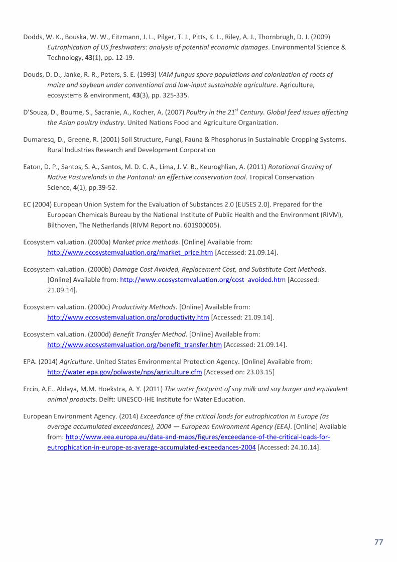
77
Dodds, W. K., Bouska, W. W., Eitzmann, J. L., Pilger, T. J., Pitts, K. L., Riley, A. J., Thornbrugh, D. J. (2009)
Eutrophication of US freshwaters: analysis of potential economic damages. Environmental Science &
Technology, 43(1), pp. 12-19.
Douds, D. D., Janke, R. R., Peters, S. E. (1993) VAM fungus spore populations and colonization of roots of
maize and soybean under conventional and low-input sustainable agriculture. Agriculture,
ecosystems & environment, 43(3), pp. 325-335.
D’Souza, D., Bourne, S., Sacranie, A., Kocher, A. (2007) Poultry in the 21st Century. Global feed issues affecting
the Asian poultry industry. United Nations Food and Agriculture Organization.
Dumaresq, D., Greene, R. (2001) Soil Structure, Fungi, Fauna & Phosphorus in Sustainable Cropping Systems.
Rural Industries Research and Development Corporation
Eaton, D. P., Santos, S. A., Santos, M. D. C. A., Lima, J. V. B., Keuroghlian, A. (2011) Rotational Grazing of
Native Pasturelands in the Pantanal: an effective conservation tool. Tropical Conservation
Science, 4(1), pp.39-52.
EC (2004) European Union System for the Evaluation of Substances 2.0 (EUSES 2.0). Prepared for the
European Chemicals Bureau by the National Institute of Public Health and the Environment (RIVM),
Bilthoven, The Netherlands (RIVM Report no. 601900005).
Ecosystem valuation. (2000a) Market price methods. [Online] Available from:
http://www.ecosystemvaluation.org/market_price.htm [Accessed: 21.09.14].
Ecosystem valuation. (2000b) Damage Cost Avoided, Replacement Cost, and Substitute Cost Methods.
[Online] Available from: http://www.ecosystemvaluation.org/cost_avoided.htm [Accessed:
21.09.14].
Ecosystem valuation. (2000c) Productivity Methods. [Online] Available from:
http://www.ecosystemvaluation.org/productivity.htm [Accessed: 21.09.14].
Ecosystem valuation. (2000d) Benefit Transfer Method. [Online] Available from:
http://www.ecosystemvaluation.org/benefit_transfer.htm [Accessed: 21.09.14].
EPA. (2014) Agriculture. United States Environmental Protection Agency. [Online] Available from:
http://water.epa.gov/polwaste/nps/agriculture.cfm [Accessed on: 23.03.15]
Ercin, A.E., Aldaya, M.M. Hoekstra, A. Y. (2011) The water footprint of soy milk and soy burger and equivalent
animal products. Delft: UNESCO-IHE Institute for Water Education.
European Environment Agency. (2014) Exceedance of the critical loads for eutrophication in Europe (as
average accumulated exceedances), 2004 — European Environment Agency (EEA). [Online] Available
from: http://www.eea.europa.eu/data-and-maps/figures/exceedance-of-the-critical-loads-for-
eutrophication-in-europe-as-average-accumulated-exceedances-2004 [Accessed: 24.10.14].

78
European Commission - EU FADN. (2013) EU cereal farms report 2012. [Online] Available from:
http://ec.europa.eu/agriculture/rica/pdf/cereal_report_2012.pdf [Accessed on: 11.03.15]
EXIOPOL. (2011) A new environmental accounting framework using externality data and input-output for
policy analysis. Bottom-up approach. European Commission Sixth Framework Programme (Project n.
037033-2)
ExternE Project. (2000) Method for Estimation of Physical Impacts and Monetary Valuation for Priority
Impact Pathways. Externalities of Energy. Oxfordshire, UK.
ExternE Project. (2003) Method for Estimation of Physical Impacts and Monetary Valuation for Priority
Impact Pathways. Externalities of Energy. Oxfordshire, UK.
FAO. (2003) Case Study No. 4 Organic Agriculture and Genetic Resources for Food and Agriculture. In:
Biodiversity and the Ecosystem Approach in Agriculture, Forestry and Fisheries. [Online] Available
from: http://www.fao.org/docrep/005/y4586e/y4586e05.htm [Accessed on: 11.03.15]
FAO. (2013) Food wastage footprint. Impacts on natural resources. Summary Report
FAO. (2014a) Food wastage footprint. Full-cost accounting. Final Report
FAO. (2014b) Table of Contents. Corporate Document Repository. Food composition table for international
use. [Online] Available from: http://www.fao.org/docrep/x5557e/x5557e00.htm#Contents
[Accessed: 22.10.14].
FAO. (2015a) Grazing management of pastures. [Online] Available from:
http://www.fao.org/ag/agp/AGPC/doc/publicat/FAOBUL4/FAOBUL4/B411.htm [Accessed: 11.02.15]
FAO. (2015b) Livestock and the environment: Finding a balance. [Online] Available from:
http://www.fao.org/ag/agp/AGPC/doc/publicat/FAOBUL4/FAOBUL4/B411.htm [Accessed: 11.02.15]
FAOSTAT. (2014a) FAOSTAT. [Online] Available from: http://faostat3.fao.org/download/Q/QV/E [Accessed:
22.10.14].
FAOSTAT. (2014b) FAOSTAT. [Online] Available from: http://faostat3.fao.org/download/Q/*/E [Accessed:
22.10.14].
FAOSTAT Emissions Database. (2014) [Online] Available from: http://faostat3.fao.org/browse/G1/*/E and
http://faostat3.fao.org/browse/G12*/E [Accessed 22.10.14]
Fears, R. (2013) Create drought-resistant pastures with holistic management. [Online] Available from:
http://www.progressivecattle.com/topics/range-pasture/5545-create-drought-resistant-pastures-
with-holistic-management [Accessed: 02.03.14]
Ferguson, B. G., Diemont, S. A., Alfaro-Arguello, R., Martin, J. F., Nahed-Toral, J., Álvarez-Solís, D., Pinto-Ruíz,
R. (2013) Sustainability of holistic and conventional cattle ranching in the seasonally dry tropics of
Chiapas, Mexico. Agricultural Systems, 120, pp. 38-48.

79
Ferraz, J. B. S., de Felicio, P. E. (2010) Production systems – An example from Brazil. Meat Science, vol. 84, no.
2, pp. 238–243.
Firbank, L. G. (2003) Introduction. Philosophical Transactions of the Royal Society of London B, 358, 1777-
1778.
Garcia, M. A., Altieri, M. A. (2005) Transgenic Crops: Implications for Biodiversity and Sustainable Agriculture.
Bulletin of Scince, Technology and Society, vol. 25, pp. 335-353.
Gerber, P.J., Steinfeld, H., Henderson, B., Mottet, A., Opio, C., Dijkman, J., Falcucci, A., Tempio, G. (2013)
Tackling climate change through livestock – A global assessment of emissions and mitigation
opportunities. Rome: Food and Agriculture Organization of the United Nations (FAO).
GMO Compass. (2014) Genetically modified plants: Global cultivation on 174 million hectares. [Online]
Available from: http://www.gmo-
compass.org/eng/agri_biotechnology/gmo_planting/257.global_gm_planting_2013.html [Accessed
on: 15.05.15]
Goedkoop, M. and Spriensma, R. (2001). The Eco-Indicator 99: A damage oriented method for Life Cycle
Impact Assessment. Methodology Annex. Amersfoort: Pre Consultant.
Hanson, J. C., Lictenberg E., Peter, S. E. (1997) Organic versus conventional grain production in the mid-
Atlantic: An economic and farming system overview. American Journal of Alternative Agriculture, 12,
2-9.
Heard, M. S., Hawes, C., Champion, G. T., Clark, S. J., Firbank, L. G., Haughton, A. J. (2003) Weeds in fields
with contrasting conventional and genetically modified herbicide tolerant crops. I. Effects on
abundance and diversity. Philosophical Transactions of the Royal Society of London, 358, 1819-1832.
Heins, B. (2011) Profitability of organic dairy farming. University of Minnesota. [Online] Available from:
http://www.extension.umn.edu/agriculture/dairy/organic/profitability-of-organic-dairy-farming/
[Accessed on: 20.04.15]
Hirschfeld, J., Weiß, J., Preidl, M. Korbun, T. (2008) Klimawirkungen der Landwirtschaft in Deutschland (The
impact of German agriculture on the climate). Discussion paper of the Institut für ökologische
Wirtschaftsforschung (IÖW), 189(8), pp. 42.
Hörtenhuber, S., Weißhaidinger, R., Lindenthal, T. (2014) Impact-characterisation for a grey water footprint-a
discussion of two new approaches. EGU General Assembly Conference Abstracts. 16, pp. 3755).
Illinois University (2015) The Science of Composting. [Online] Available from:
http://web.extension.illinois.edu/homecompost/science.cfm [Accessed: 02.03.14]
IPCC. (2007) IPCC Fourth Assessment Report: Climate Change 2007. Climate Change 2007: Working Group III:
Mitigation of Climate Change. 2.4 Cost and benefit concepts, including private and social cost
perspectives and relationships to other decision-making frameworks.

80
Interagency Working Group on Social Cost of Carbon, United States Government. (2013). Technical Update of
the Social Cost of Carbon for Regulatory Impact Analysis.
InterDev. (2015) Agroecological Farming Systems. InterDev Natural Resource Management. [Online]
Available from: http://www.fao.org/docs/eims/upload/207703/fiche%20WP3.pdf [Accessed:
10.02.15]
Jain, N., Dubey, R., Dubey, D. S., Singh, J., Khanna, M., Pathak, H., Bhatia, A. (2014) Mitigation of greenhouse
gas emission with system of rice intensification in the Indo-Gangetic Plains. Paddy and water
environment, 12(3), pp. 355-363.
Jayapalreddy, R., Shenoy N. S. (2013) A comparative economic analysis of Traditional and System of Rice
Intensification (SRI) rice cultivation practices in Mahabubnagar district of Andhra Pradesh.
International Journal of Scientific and Research Publications. 3 (10), pp. 404-409.
Jeffries, P., Gianinazzi, S., Perotto, S., Turnau, K., Barea, J. M. (2003) The contribution of arbuscular
mycorrhizal fungi in sustainable maintenance of plant health and soil fertility. Biology and fertility of
soils, 37(1), pp. 1-16.
Jikkham, P., Wongyala, P. (2015) ‘RID issues drought alert’, Bangkok Post 6 February. [Online] Available from:
http://www.bangkokpost.com [Accessed: 05.03.15].
Jung, C. G., Park J. Y., Kim, S. J., Park, G. A. (2014) The SRI (system of rice intensification) water management
evaluation by SWAPP (SWAT–APEX Program) modeling in an agricultural watershed of South Korea.
Paddy Water Environment, 12, pp. 251-261.
Kaimowitz, D., Mertens, B., Wunder, S., Pacheco, P. (2004) Hamburger connection fuels Amazon destruction.
Bangor, Indonesia. Bogor. Center for International Forest Research. [Online] Available from:
http://www.herbogeminis.com/IMG/pdf/hamburger_connection.pdf [Accessed on: 11.06.15]
Katakey, R., Chaudhary, A. (2013) Cancer Express Carries Sufferers of India’s Deadly Waters. Bloomberg
Business. [Online] Available from: http://www.bloomberg.com/news/articles/2013-10-28/cancer-
express-carries-sufferers-of-india-s-deadly-waters [Accessed: 09.03.15]
Klonsky, K. (2012) Comparison of Production Costs and Resource Use for Organic and Conventional
production systems. American Journal of Agricultural economics, 94, 314-321.
Kumar, K. Goh, K. M. (2002) Management practices of antecedent leguminous and non-leguminous crop
residues in relation to winter wheat yields, nitrogen uptake, soil nitrogen mineralization and simple
nitrogen balance. European Journal of Agronomy, 16(4), pp. 295-308.
Larson, D. (2013) Cover Crops Bring a Diversity of Benefits to the Farm. [Online] Available from:
http://mosesorganic.org/farming/farming-topics/field-crops/cover-crops-bring-a-diversity/
[Accessed on: 27.02.15]
Latour, J. B., Staritsky, I. G, Alkemade, J. R. M., Wietrz, J., (1997) De natuurplanner. Decision support system
natuur en milieu. RIVM report 711901019

81
Leake, J., Johnson, D., Donnelly, D., Muckle, G., Boddy, L., Read, D. (2004) Networks of power and influence:
the role of mycorrhizal mycelium in controlling plant communities and agroecosystem functioning.
Canadian Journal of Botany, 82(8), pp. 1016-1045.
Livestock, Environment and Development (LEAD) Initiative. (2015). Livestock and Environment Toolbox. Food
and Agriculture Organisation of the United Nations [Online] Available from:
http://www.fao.org/ag/againfo/programmes/en/lead/toolbox/Indust/IndPProd.htm [Accessed:
10.02.15]
Lijzen, J.P.A., Rikken, M.G.J. (eds.). (2004) EUSES: European Union System for the Evaluation of Substances,
Version 2.0, Background Report. RIVM Report no. 601900005/2004
Lovei, G. L. (2001) Ecological risks and benefits of transgenic plants. New Zealand Plant Protection, 54, 93-
100.
MA. (2005) Millennium Ecosystem Assessment. Ecosystems and Human Well-being: Synthesis. Island Press,
Washington, DC.
Mäder, P., S. Edenhofer, T. Boller, A. Wiemken Niggli, U. (2000) Arbuscular mycorrhizae in a long-term field
trial comparing low-input (organic, biological) and high-input (conventional) farming systems in a
crop rotation. Biol. Ferti. Soils, 31, pp. 150-156.
Mäder, P., Fliessbach, A., Dubois, D., Gunst, L., Fried, P., Niggli, U. (2002) Soil fertility and biodiversity in
organic farming. Science, 296(5573), pp. 1694-1697.
McBride, W. D., Greene, C. (2009) The profitability of organic soybean production. Renewable agriculture and
food systems, 24(04), pp. 276-284.
McCoy, S. (2005) Organic wheat – production system guidelines. [Online] Available from:
http://archive.agric.wa.gov.au/objtwr/imported_assets/content/fcp/cer/wh/cp/f13700.pdf
[Accessed on: 26.02.15]
McDonald, R., Shemie, D. (2014) Urban Water Blueprint: Mapping conservation solutions to the global water
challenge, Washington, D.C.: The Nature Conservancy.
McWilliams, J. E. (2013) All Sizzle and No Steak – Why Allan Savory’s TED talk about how cattle can reverse
global warming is dead wrong. [Online] Available from:
http://www.slate.com/articles/life/food/2013/04/allan_savory_s_ted_talk_is_wrong_and_the_bene
fits_of_holistic_grazing_have.html [Accessed on: 04.03.15]
Meier, M. S., Jungbluth, N., Stoessel, F., Schader, C. Stolze M. (2014) Higher accuracy in N modelling makes a
difference. In: 9th International Conference LCA of Food 8-10 October 2014, San Francisco, USA.
Meier, M. S., Jungbluth, N., Stoessel, F., Schader, C. Stolze M. (2014) Higher accuracy in N modelling makes a
difference. In: 9th International Conference LCA of Food 8-10 October 2014, San Francisco, USA.
82
Meier, M. S., Stoessel, F., Jungbluth, N., Juraske, R., Schader, C., Stolze, M. (2015) Environmental impacts of
organic and conventional agricultural products - Are the differences captured by life cycle
assessment? Journal of Environmental Management. 149, 193-208
Mekonnen, M.M. and Hoekstra, A.Y. (2011) The green, blue and grey water footprint of crops and derived
crop products, Value of Water Research Report Series. No. 47, UNESCO-IHE, Delft, the Netherlands.
Nemes, N. (2009) Comparative Analysis of Organic and Non-Organic Farming Systems: A Critical Assessment
of Farm Profitability. Food and Agriculture Organization of the United Nations. Natural Resource
Management and Environment Department.
Nepstad, D. C., Stickler, C. M., Almeida, O. T. (2006) Globalization of the Amazon soy and beef industries:
opportunities for conservation. Conservation Biology, vol. 20, no. 6, pp. 1595–1603.
New Energy Externalities Developments for Sustainability (NEEDS). (2006) Assessment of Biodiversity Losses.
Sixth Framework Programme. Zurich: Econcept AG.
NCC. (2014a) What is Natural Capital. [Online] Available from: http://www.naturalcapitalcoalition.org/why-
natural-capital/natural-capital.html [Accessed 20.12.14]
NCC. (2014b) Developing the Protocol. [Online] Available from:
http://www.naturalcapitalcoalition.org/natural-capital-protocol/developing-the-protocol.html
[Accessed 20.12.14]
NCSPA. (2014) Uses of Soybeans. [Online] Available from: http://ncsoy.org/media-resources/uses-of-
soybeans/ [Accessed: 09.03.15]
NLWRA. (2008) The Australian beef industry. Australian Government National Land and Water Resources
Audit.
Ometto, J. P., Sampaio, G., Marengo, J., Assis, T., Tejada, G., Aguiar, A. P. (2013) Climate Change and Land
Use Change in Amazonia. Report for Global Canopy Programme and International Center for Tropical
Agriculture as part of the Amazonia Security Agenda project.
Opio, C., Gerber, P., Mottet, A., Falcucci, A., Tempio, G., MacLeod, M., Vellinga, T., Henderson, B. Steinfeld,
H. (2013) Greenhouse gas emissions from ruminant supply chains – A global life cycle assessment.
Food and Agriculture Organization of the United Nations (FAO).
Palanisami, K., Karunakaran, K. R., Amarasinghe, U. (2012) Impact of the System of Rice Intensification (SRI)
Analysis of SRI Practices in 13 States of India. [Online] Available from:
http://www.iwmi.cgiar.org/iwmi-tata/PDFs/2012_Highlight-07.pdf [Accessed: 12.03.15]
Pfister, S., Koehler, H., Hellweg, S. (2009) Assessing the Environmental Impacts of Freshwater Consumption in
LCA. ETH Zurich, Institute of Environmental Engineering. Environmental Science and Technology 43,
4098-4104.
Pimentel, D., Hepperly, P., Hanson, J., Douds, D., Seidel, R. (2005) Environmental, Energetic, and Economic
Comparisons of Organic and Conventional Farming Systems. BioScience, 55, 573-582.

83
Pimentel, D. (2006) Impacts of Organic Farming on the Efficiency of Energy Use in Agriculture. Ithaca: Cornell
University.
Ponisio, L. C., M’Gonigle, L. K., Mace, K. C., Palomino, J., de Valpine, P., Kremen, C. (2014) Diversification
practices reduce organic to conventional yield gap. The Royal Society. Proceedings B. 282.
PRI. (2014) PRI-Coordinated engagement on water risks in agricultural supply chains. Investor Guidance
Document. In collaboration with: WWF, PwC Germany and the PRI investor steering committee on
water risks.
Rajendran, R., Ravi, V., Chelliah, N., Balasubramanian, V. (2007) Individual and combined effect of
management components of SRI on the productivity of irrigated rice. Unpublished presentation at:
2nd National SRI Symposium, October 3-5, 2007, Agartala, Tripura State, India.
Royal Horticultural Society. (2015) Mycorrhizal Fungi. [Online] Available from:
https://www.rhs.org.uk/advice/profile?pid=633 [Accessed on: 13.03.15]
Rubinos, R., Jalipa, A. T., Bayacag, P. (2007) Comparative Economics Study of Organic and Conventional Rice
Farming in Magsaysay, Davao del Sur. 10th National Convention on Statistics (NCS).
Salon, P. (2012) Diverse Cover Crop Mixes for Good Soil Health. Corning: USDA-NRCS.
SARE. (2012) Crop Rotation with Cover Crops [Online] Available from: http://www.sare.org/Learning-
Center/Books/Managing-Cover-Crops-Profitably-3rd-Edition/Text-Version/Crop-Rotation-with-
Cover-Crops [Accessed on: 27.02.15]
Savory, A. (2013) Response to request for information on the “science” and “methodology” underpinning
Holistic Management and holistic planned grazing. [Online] Available from:
http://www.savoryinstitute.com/media/42448/Science-Methodology-Holistic-
Mgt_Update_March.pdf [Accessed on: 16.03.15]
Savory Institute (2013) Restoring the Climate through Capture and Storage of Soil Carbon through Holistic
Planned Grazing. [Online] Available from:
http://www.savoryinstitute.com/media/40591/Savory_Institute_Carbon_RestoringClimateWhitePap
er_April2013.pdf [Accessed: 02.03.15]
SimaPro. (2014a) Agri-footprint library. PRé-sustainability.
SimaPro. (2014b) Ecoinvent library. PRé-sustainability.
SimaPro. (2014c) Pfister’s characterization model. PRé-sustainability.
SimaPro. (2014d) ReCiPe. PRé-sustainability.
Soyatech. (2015) Soy Facts. Soyatech LLC. [Online] Available from: http://www.soyatech.com/soy_facts.htm
[Accessed on: 05.05.15]
84
Stern, N. (2006) Stern Review Report on the Economics of Climate Change. [Online] Available from:
http://mudancasclimaticas.cptec.inpe.br/~rmclima/pdfs/destaques/sternreview_report_complete.p
df [Accessed on: 03.12.14]
Teague, W. R., Dowhower, S. L., Baker, S. A., Haile, N., DeLaune, P. B., Conover, D. M. (2011) Grazing
management impacts on vegetation, soil biota and soil chemical, physical and hydrological properties
in tall grass prairie. Agriculture, Ecosystems & Environment, 141(3), pp. 310-322.
TEEB Brazil. (2014) TEEB for Business Brazil – Final Report
TEEB for Business Coalition. (2013) Natural Capital at Risk: The Top 100 Externalities of Business
Thiyagarajan, T. M., Gujja, B. (2013) SRI Transforming Rice Production with SRI (System of Rice Intensification)
Knowledge and Practice. [Online] Available from:
http://www.agsri.com/images/documents/sri/sri_book_final_version.pdf [Accessed: 24.02.15]
Tol, R. (2011) The Social Cost of Carbon. Annual Review of Resource Economics, Annual Reviews, 3(1), p. 419-
443.
Townsend, A. R., Howarth, R. W., Bazzaz, F. A., Booth, M. S. Cleveland, C. C. (2003) Human Health Effects of a
Changing Global Nitrogen Cycle. Frontiers in Ecology and the Environment, 1(5), pp. 240-246.
Undersander, D., Albert, B., Cosgrove, D., Johnson, D., Peterson, P. (2002) Pastures for Profit: A Guide to
Rotational Grazing (A3529), Madison: Cooperative Extension Publishing
UNEP. (2007) Global Environment Outlook GEO-4: Environment for development. United Nations
Environment Programme.
UNEP. (2010) Our Planet. Natural Capital - The Economics of Ecosystems and Biodiversity. United Nations
Environment Programme.
US EPA. (2003) Tool for the Reduction and Assessment of Chemical and Other Environmental Impacts (TRACI):
User’s Guide and System Documentation. EPA/600/R-02/052.
US EPA. (2013) The Social Cost of Carbon. [Online] Available from:
http://www.epa.gov/climatechange/EPAactivities/economics/scc.html [Accessed 22.12.14]
UNEP. (2012) Avoiding Future Famines: Strengthening the Ecological Foundation of Food Security through
Sustainable Food Systems. United Nations Environment Programme (UNEP), Nairobi, Kenya.
van der Heijden, M. G., Klironomos, J. N., Ursic, M., Moutoglis, P., Streitwolf-Engel, R., Boller, T., Wiemken, A.
Sanders, I. R. (1998). Mycorrhizal fungal diversity determines plant biodiversity, ecosystem variability
and productivity. Nature, 396(6706), pp. 69-72.
Van der Ploeg, S. and R.S. de Groot. (2010) The TEEB Valuation Database – a searchable database of 1310
estimates of monetary values of ecosystem services. Foundation for Sustainable Development,
Wageningen, the Netherlands.

85
Van Zelm R, Huijbregts MAJ, Van de Meent D. (2009) EUSES-LCA 2.0: a global nested multi-media fate,
exposure and effects model. J LCA 14: 282-284.
Walls, M. (2006) Agriculture and Environment. European Commission. [Online] Available from:
http://ec.europa.eu/research/agriculture/scar/pdf/scar_foresight_environment_en.pdf [Accessed
on: 23.03.15]
Way, M. J., Heong, K.L. (1994) The role of biodiversity in the dynamics and management of insect pests of
tropical irrigated rice—a review. Bulletin of Entomological Research, 84, pp. 567-587.
Weber, C., Neumeister, L. Ruhnau, M. Mücke, M. (2002) From Law to Field Pesticide Use Reduction in
Agriculture - From Pesticide Residue Analyses to Action (Executive Summary). Hamburg: Pesticide
Action Network Germany.
WHO. (1999) The state of the environment; freshwater. GEO-2000: Global Environment Outlook. Nairobi:
United Nations Environment Programme.
WHO. (2002) The World Health Report 2002: Reducing Risks, Promoting Healthy Life. Geneva: World Health
Organization.
Wibbelmann, M., Schmutz, U., Wright, J., Udall, D., Rayns, F., Kneafsey, M., Trenchard, L., Bennett, J.,
Lennartsson, M. (2013) Mainstreaming Agroecology: Implications for Global Food and Farming
Systems. Centre for Agroecology and Food Security Discussion Paper. Coventry: Centre for
Agroecology and Food Security. ISBN: 978-1-84600-0454
Wilson, G. W., Rice, C. W., Rillig, M. C., Springer, A. Hartnett, D. C. (2009) Soil aggregation and carbon
sequestration are tightly correlated with the abundance of arbuscular mycorrhizal fungi: results from
long‐term field experiments. Ecology Letters, 12(5), pp. 452-461.
WRI. (2014) Wetting and drying: Reducing greenhouse gas emissions and saving water from rice production.
Installment 8 of “Creating a Sustainable Food Future”. Working Paper. World Resources Institute.
WWF. (2012) The 2050 Criteria: Guide to Responsible Investment in Agricultural, Forest and Seafood
commodities.
Wynen, E. (2001) The economics of organic cereal–livestock farming in Australia revisited. Australian
Agricultural and Resource Economics Society.
Zhao, L., Wu, L., Dong, C., Li, Y. (2010a) Rice yield, nitrogen utilization and ammonia volatilization as
influenced by modified rice cultivation at varying nitrogen rates. Agricultural Sciences. 1 (1), pp. 10-
16.
Zhao, L., Wu, L., Li, Y., Animesh, S., Zhu, D., Uphoff, N. (2010b) Comparisons of yield, water use efficiency, and
soil microbial biomass as affected by the system of rice intensification. Communications in soil
science and plant analysis, 41(1), pp. 1-12.

86
APPENDIX I: NATURAL CAPITAL PROTOCOL
The Food and Beverage Sector Guide, in conjunction with the main Natural Capital Protocol, are
currently in an early drafting phase but are expected to contain the following sections (or a variation
thereof):
SECTOR SPECIFIC CONTEXT
Background on why natural capital is relevant to the Food and Beverage sector and how the
sector benefits from it.
The business case for natural capital measurement in the sector which will include:
o Engagement with key stakeholders;
o Overview of the key business value drivers and benefits of conducting a natural capital
assessment.
Sector Materiality Matrix: will define the material natural capital impacts and dependencies at
each stage of the value chain for different sectors and subsectors.
PRACTICAL GUIDANCE FOR APPLYING THE NCP AND FOOD AND BEVERAGE GUIDES
This will follow the principles outlined in the NCP but provide any sector-specific considerations
where relevant.
PRACTICAL CASE STUDIES
Demonstrate how the NCP has been applied within the food and beverages sector.
Demonstrate how the NCP has addressed specific business value drivers and delivered business
benefits.
Demonstrate how businesses can embed the NCP on an ongoing basis.

87
APPENDIX II: NATURAL CAPITAL INTENSITIES PER
REVENUE
Tables 19 and 20 below outline the natural capital intensities of the commodities included in this study.
They show the total cost of natural capital impacts, per million USD revenue generated by each sector in
the countries shown. This is to supplement the information presented throughout this study which
presents natural capital intensities in terms of USD per tonne of production. The table also shows the
natural capital impacts as a percentage of the revenue in each sector and country. The cost of natural
capital impacts as a percentage of revenue range between 111 percent and 893% for crop farming, and
between 42% and 1 237% for livestock farming. The sectors with the highest median natural capital cost
as a percentage of revenue is rice farming (378 percent) for crops, and beef production (280 percent)
for livestock.
TABLE 19: NATURAL CAPITAL INTENSITIES OF CROP PRODUCTION
Rank Country Cost of natural capital impacts
per USD million revenue
(USD per USD million)
Cost of natural capital
impacts as a percentage of
revenue
Maize production
1 France 5 881 824 588%
2 Brazil 3 818 542 382%
3 India 2 780 742 278%
4 Ukraine 2 706 300 271%
5 Mexico 2 555 130 256%
6 Indonesia 2 395 964 240%
7 China 1 986 186 199%
8 Argentina 1 308 860 131%
9 Canada 1 210 528 121%
10 USA 1 113 071 111%
Rice production
1 Bangladesh 4 959 970 496%
2 Viet Nam 4 021 171 402%
3 Myanmar 3 905 496 391%
4 Thailand 3 782 572 378%
5 Indonesia 2 285 902 229%
6 India 1 744 003 174%
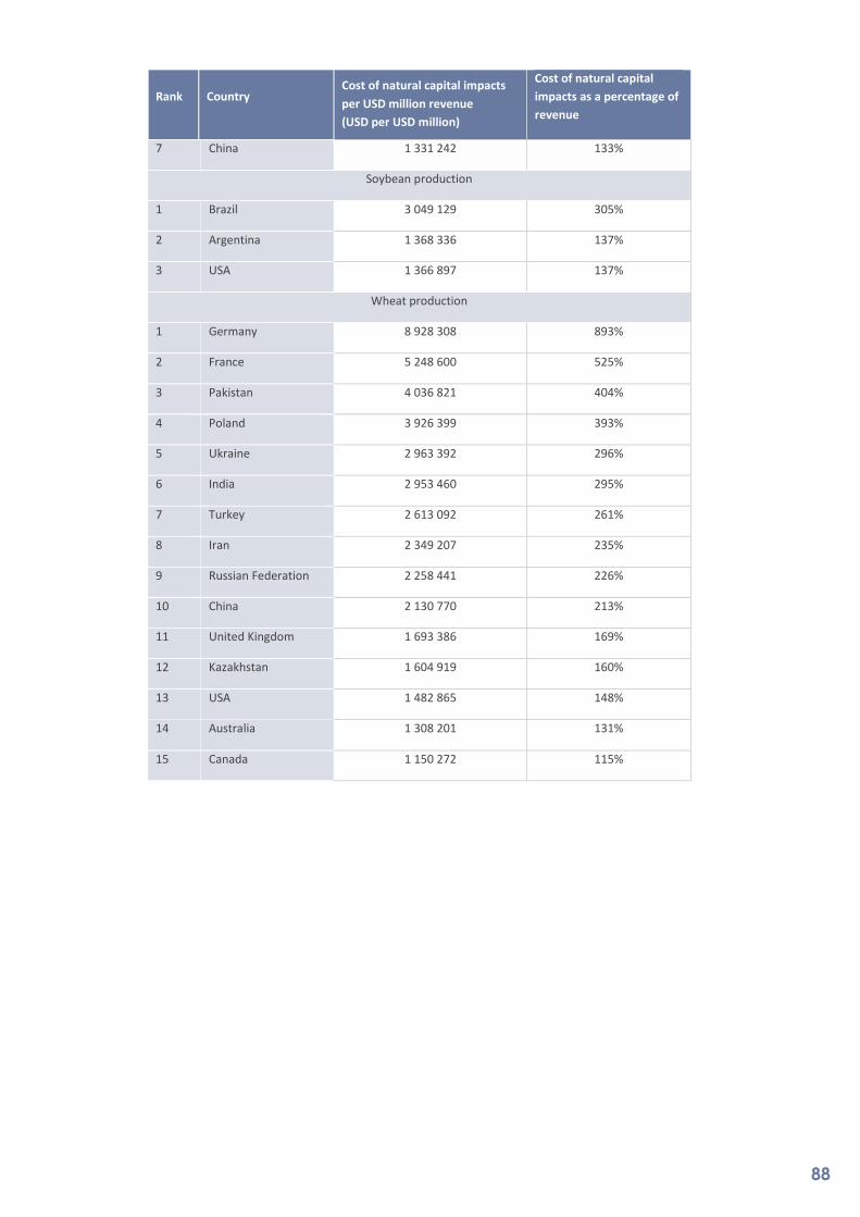
88
Rank Country Cost of natural capital impacts
per USD million revenue
(USD per USD million)
Cost of natural capital
impacts as a percentage of
revenue
7 China 1 331 242 133%
Soybean production
1 Brazil 3 049 129 305%
2 Argentina 1 368 336 137%
3 USA 1 366 897 137%
Wheat production
1 Germany 8 928 308 893%
2 France 5 248 600 525%
3 Pakistan 4 036 821 404%
4 Poland 3 926 399 393%
5 Ukraine 2 963 392 296%
6 India 2 953 460 295%
7 Turkey 2 613 092 261%
8 Iran 2 349 207 235%
9 Russian Federation 2 258 441 226%
10 China 2 130 770 213%
11 United Kingdom 1 693 386 169%
12 Kazakhstan 1 604 919 160%
13 USA 1 482 865 148%
14 Australia 1 308 201 131%
15 Canada 1 150 272 115%

89
TABLE 20: NATURAL CAPITAL INTENSITIES OF LIVESTOCK PRODUCTION
Rank Country
Cost of natural capital impacts
per USD million revenue
(USD per USD million)
Cost of natural capital
impacts as a percentage of
revenue
Cattle (beef) production
1 Venezuela 12 367 482 1237%
2 Brazil 11 834 766 1183%
3 Mexico 8 027 546 803%
4 Colombia 6 677 780 668%
5 Australia 3 959 908 396%
6 Pakistan 3 513 580 351%
7 Argentina 3 449 738 345%
8 China 3 443 982 344%
9 Spain 2 896 132 290%
10 Uzbekistan 2 886 315 289%
11 Uruguay 2 814 861 281%
12 South Africa 2 805 845 281%
13 Poland 2 797 216 280%
14 Canada 2 665 919 267%
15 Egypt 2 647 451 265%
16 New Zealand 2 640 853 264%
17 USA 2 621 086 262%
18 Ireland 2 537 506 254%
19 France 2 329 415 233%
20 United Kingdom 2 252 338 225%
21 Russian Federation 2 122 764 212%
22 Germany 2 050 332 205%
23 Turkey 1 718 306 172%
24 Italy 1 679 379 168%
25 Japan 1 349 206 135%
Cattle (dairy) production
1 Iran 2 823 922 282%
2 Brazil 1 966 547 197%
3 Mexico 1 908 054 191%

90
Rank Country
Cost of natural capital impacts
per USD million revenue
(USD per USD million)
Cost of natural capital
impacts as a percentage of
revenue
4 Uzbekistan 1 684 474 168%
5 Colombia 1 566 449 157%
6 India 1 548 286 155%
7 Ecuador 1 373 288 137%
8 Pakistan 1 354 228 135%
9 Belarus 1 340 241 134%
10 Poland 1 202 680 120%
11 Australia 1 158 632 116%
12 Argentina 1 143 108 114%
13 Ukraine 1 137 245 114%
14 Russian Federation 1 113 216 111%
15 China 1 100 400 110%
16 USA 1 076 352 108%
17 Turkey 1 027 387 103%
18 United Kingdom 955 007 96%
19 France 936 465 94%
20 New Zealand 929 681 93%
21 Spain 909 797 91%
22 Germany 884 526 88%
23 Italy 834 692 83%
24 Canada 804 286 80%
25 Netherlands 800 538 80%
26 Japan 702 434 70%
Pork production
1 Netherlands 4 585 539 459%
2 Denmark 3 797 541 380%
3 Philippines 2 333 527 233%
4 Brazil 1 476 549 148%
5 Germany 1 334 506 133%
6 Spain 964 392 96%
7 China 850 945 85%

91
Rank Country
Cost of natural capital impacts
per USD million revenue
(USD per USD million)
Cost of natural capital
impacts as a percentage of
revenue
8 France 842 811 84%
9 USA 547 525 55%
10 Viet Nam 509 593 51%
11 Canada 486 422 49%
12 Russian Federation 422 072 42%
Poultry production
1 Myanmar 1 488 302 149%
2 China 1 488 153 149%
3 India 1 445 707 145%
4 Thailand 1 390 634 139%
5 Argentina 1 365 990 137%
6 South Africa 1 300 396 130%
7 Turkey 1 262 818 126%
8 Mexico 1 256 759 126%
9 Brazil 1 229 378 123%
10 USA 1 224 734 122%
11 Malaysia 1 214 700 121%
12 France 1 164 566 116%
13 Iran 1 164 418 116%
14 United Kingdom 1 163 522 116%
15 Germany 1 133 607 113%
16 Australia 1 133 323 113%
17 Peru 1 123 916 112%
18 Indonesia 1 122 426 112%
19 Poland 1 121 568 112%
20 Canada 1 089 826 109%
21 Colombia 1 077 150 108%
22 Spain 1 071 814 107%
23 Japan 1 046 979 105%
24 Russian Federation 1 045 271 105%

92
APPENDIX III: TRUCOST’S ENVIRONMENTALLY
EXTENDED INPUT-OUTPUT (EEIO) MODEL
Environmental impacts directly attributable to a business are calculated according to Trucost’s
environmental matrix, which contains expenditure information and environmental intensities per unit
of output across 531 sectors within and beyond agriculture. The environmental expenditures are used in
conjunction with the environmental intensities in order to model the impacts across the economy
associated with the activity of a company within one of these sectors. The environmental data that is
used within the EEIO comes from a number of sources including FAO, LCA databases such as Agri-
Footprint and UNFCCC. Trucost has been collecting environmental data since 2000, and is therefore able
to test this model based against 15 years of data on quantitative environmental disclosures, from
thousands of companies, which analysts engage with annually.
The EEIO can be segregated into two parts: the ‘direct’ and ‘indirect’ models. The direct model
estimates the impacts resulting from the operations of a business, for example, the emissions coming
from on-site fuel use or the impacts associated with applying fertilizers. The indirect model estimates
the impacts from the activities from upstream suppliers. These are businesses that produce the inputs
so that a business can operate. This can include the impacts associated with producing fertilizers,
pesticides as well as the transportation of purchased goods. More details on the direct and indirect
models can be found below.
TABLE 21: THE KEY COMPONENTS OF TRUCOST’S EEIO
Component Justification
Indirect Model
Input-Output (IO) Factors
IO factors for the flow of goods and services between sectors are created from United
States Bureau of Economic Analysis (BEA) benchmark supply and use tables.18
These are
produced to enable government and business decision-makers, researchers, and the
general public to track and understand the performance of the US economy.
Direct Model Environmental Matrix
The environmental impacts of sectors are calculated using country-specific impact factors.
Market traded commodities extracted and water resources are measures at a local level.
18 http://www.bea.gov/industry/io_benchmark.htm

93
Indirect Model
Indirect or supply chain impacts are calculated from supply and use tables published by the United
States Department of Commerce, Bureau of Economic Analysis (BEA)19. BEA compiles data from a wide
range of sources including the Economic Census (conducted every 5 years) and annual surveys for
specific industries including the agricultural, mining, manufacturing, wholesale trade, retail trade,
transportation, communications, and utilities, finance, insurance and real estate surveys. Data is
collated and homogenized so that each industry’s inputs reflect, as far as possible, a unique set of inputs
for around 426 industries.
Input-output tables are created detailing the ratio of expenditure from one sector with every other
sector of the economy, termed “intermediate demands”. It is largely due to this level of detail that
Trucost has chosen to use the USA economy as a proxy for the world economy as a starting point for the
creation of its indirect model. Additionally, the U.S. economy has the advantage of being highly
diversified, so major commodities can be included.
However, some sectors which are important from an environmental perspective, such as power
generation, are highly aggregated, and BEA data have insufficient detail on many sectors within the
agricultural industry. In these cases, Trucost has disaggregated the input-output tables proportionally.
For example, power generation is represented by seven separate sectors within the Trucost model.
Trucost has further extended the indirect model to create indirect input-output factors for an additional
80 sectors, as well as incorporating life cycle analysis and process benchmark data. Finally, the indirect
model is refined by disclosures to Trucost from its universe of over 4 500 companies, which is collected
through an annual engagement programme.
Direct Model
Each sector within the environmental matrix contains an average impact per dollar of output for over
100 impacts which are derived from governmental, life cycle assessment and academic data. Trucost
tests this data against the many thousands of disclosures it collects from companies during the annual
engagement programme.
The sources used to determine direct factors for agricultural sectors are described below. Non-energy
related greenhouse gases data has been sourced from FAOSTAT Emissions Database on a country-by-
country basis, based on IPCC Tier 1 Guidelines. Simapro’s Agri-footprint library (SimaPro, 2014a), and
Ecoinvent library (SimaPro, 2014b) were used to quantify energy related greenhouse gases emissions
and air pollutants. Water consumption was determined using data from Mekonnen and Hoekstra (2010)
at a country level (which produced similar results to the blue water footprints that can be found on
AQUASTAT). Land use for ruminants was estimated using the SOL-model (FAO, 2013). Land use for
poultry was calculated combining the distribution of intensive and extensive systems for different
regions (FAO and ILRI, 2011) and respective animal densities (FAO, 2004; LEI Wageningen UR, 2013).
Land use for crops was calculated using harvested area per country, taken from FAOSTAT (2011a).
Fertilizer use factors were determined using FertiStat (2007) and IFA (2009). Pesticide use factors were
19 http://www.bea.gov/industry/io_annual.htm

94
determined using NCFAP (2008) and FAO (2009). Production quantities and price of commodities per
country were sourced from FAOSTAT (2011a; 2011b).
Where available, Trucost applied country specific factors. Otherwise, global average factors were
applied, weighted by production value.
Outputs and Externalities
Trucost’s EEIO outputs cover over 100 environmental impacts which can be condensed into 6 high-level
environmental key performance indicators covering the major categories of unpriced natural capital
impact categories: water use, greenhouse gas emissions (GHGs), waste, air pollution, land and water
pollution, and land use change.
Strengths and Weaknesses
Input-Output (IO) modelling assumes generic flows behind sectors, as described in the indirect model
above. On a global basis, this can be adjusted using multi-regional IO modelling, or a hybrid approach as
suggested for this project.
Multi-regional IO modelling adjusts for trade between regions to estimate embedded impacts in
products more accurately. Trucost recommends adopting a hybridized approach to adjust for regional
variations in environmental impacts as described above. This is because single region IO models have
greater granularity: Trucost’s EEIO model includes 531 sectors whereas multi-regional IO models usually
include 80 sectors.
Appendix III References
FAO (2004) Small- scale poultry production. Technical guide. Rome: Food and Agriculture Organization
of the United Nations.
FAO. (2013) Impact of a global upscaling of low-input and organic livestock production. Sustainability
and Organic Livestock Model (SOL-m). Food and Agriculture Organisation of the United Nations.
FAOSTAT. (2009) Agri-Environmental Indicators. Pesticides. [Online] Available from:
http://faostat3.fao.org/download/E/EP/E [Accessed on: 22.10.14]
FAOSTAT. (2011a) Production. [Online] Available from: http://faostat3.fao.org/browse/Q/*/E [Accessed
on: 22.10.14]
FAOSTAT. (2011b) Producer prices. [Online], Available from: http://faostat3.fao.org/download/P/PP/E
[Accessed on: 22.10.14]
FAO and ILRI. (2011) Global livestock production systems. Rome: Food and Agriculture Organization of
the United Nations (FAO) and International Livestock Research Institute (ILRI).

95
FertiStat. (2007) Fertilizer use statistics. Plant Production and Protection Division, FAO. [Online],
Available from: http://www.fao.org/ag/agp/fertistat [Accessed on: 22.10.14]
IFA. (2009) International Fertilizer Industry Association. [Online], Available from:
http://www.fertilizer.org [Accessed on: 22.10.14]
LEI Wageningen. (2013) Competitiveness of the EU poultry meat sector. [Online], Available from:
http://www.avec-poultry.eu/system/files/archive/new-
structure/avec/Communication/Study%20final%20version.pdf [Accessed on: 22.10.14]
Mekonnen, M. M., Hoekstra, A. Y. (2010) The green, blue and grey water footprint of farm animals and
animal products. Value of Water Research Report Series No.48, UNESCO-IHE.
NCFAP. (2008) Pesticide use database. National Center for Food and Agricultural Policy. [Online]
Available from: http://www.ncfap.org/pesticideuse.html [Accessed on: 22.10.14]
SimaPro. (2014a) Agri-footprint library. PRé-sustainability.
SimaPro. (2014b) Ecoinvent library. PRé-sustainability.

96
APPENDIX IV: KEY CONCEPTS RELATED TO NATURAL
CAPITAL VALUATIONS
Valuation Techniques
Table 22 summarizes the different techniques that can be used to value environmental impacts,
including comments on which was applied for valuing specific receptors. All of the approaches below
are equally valid, and this study chose valuation techniques best suited to calculating the social impact
of environmental emissions, taking data availability and suitability into account. The study is consistent
in its application of valuation techniques for receptors across all impact categories, for example, the
impact on crops was valued in the same manner for acidification potential and photochemical ozone
creation potential. The valuation technique selected for each environmental impact category is
provided in the valuation methodology sections that follow.
TABLE 22: VALUATION TECHNIQUES
Valuation
Technique Description
Abatement cost The cost of removing a negative by-product for example, by reducing the emissions or limiting their
impacts.
Avoided cost /
Replacement cost /
Substitute cost
Estimates the economic value of ecosystem services based on either the costs of avoiding damages
due to lost services, the cost of replacing ecosystem services, or the cost of providing substitute
services. Most appropriate in cases where damage avoidance or replacement expenditures have or
will be made (Ecosystem valuation, 2000a).
Contingent
valuation
A survey-based technique for valuing non-market resources. This is a stated preference/willingness-
to-pay model in that the survey determines how much people will pay to maintain an
environmental feature.
Direct market
pricing
Estimates the economic value of ecosystem products or services that are bought and sold in
commercial markets. This method uses standard economic techniques for measuring the economic
benefits from marketed goods based on the quantity purchased and supplied at different prices.
This technique can be used to value changes in the quantity or quality of a good or service
(Ecosystem valuation, 2000b).
Hedonic pricing Estimates the economic value of ecosystem services that directly affect the market price of another
good or service. For example proximity to open space may affects the price of a house.
Production function
Estimates the economic value of ecosystem products or services that contribute to the production
of commercially marketed goods. Most appropriate in cases where the products or services of an
ecosystem are used alongside other inputs to produce a marketed good (Ecosystem valuation,
2000c).
Site choice / Travel
cost method
A revealed preference/willingness-to-pay model which assumes people make trade-offs between
the expected benefit of visiting a site and the cost incurred to get there. The cost incurred is the
person’s willingness to pay to access a site. Often used to calculate the recreational value of a site.

97
Impact Pathway Approach (IPA)
IPA was used to value Eutrophication Potential, Acidification Potential and Photochemical Ozone
Creation Potential.
The Impact Pathway Approach (IPA) is a bottom-up-approach in which environmental benefits and costs
are estimated by following the pathway from the source of an environmental pressure (i.e. emission of
pollutants), via changes in the quality of air, soil and water, to the physical impact (i.e. health risks) of
such changes expressed in monetary terms.
FIGURE 28: IMPACT PATHWAY APPROACH
Environmental pressures are translated into physical impacts using dose-response functions (DRFs).
DRFs use scientific data to measure the relationship between a concentration of a pollutant (the dose)
and its impact on things like human health, building materials, crops (the receptor). The receptor
density (i.e. population density and crop density) drives the quantity of physical impact.
The study uses existing dispersion models from Life Cycle Analysis characterization models such as
SimaPro’s EcoIndicator99 (2014d) or ReCiPe (2014e), with DRF functions built-in. To account for the
variability in receptor density when building its valuation methodologies, valuations are adjusted
according to regional receptor densities, such as background population structure or air pollutant
concentration.
Value Transfer
In order to estimate environmental costs or benefits in a context when no study exists, value transfer is
used. In this method, the goal is to estimate the economic value of ecosystem services, or
environmental impacts, by transferring available information from completed studies, to another
location or context by adjusting for certain variables. Examples include population density, income
levels, and average size of ecosystems to name just a few.
Best practice guidelines for value transfers have been set-out by UNEP in a document entitled Guidance
Manual on Value Transfer Methods for Ecosystem Services (Brander, 2013). Where possible, this study
endeavoured to follow these guidelines in all of its value transfer calculations. It is important to note
however, that value transfers can only be as accurate as the initial study (Ecosystem valuation, 2000d),
and due to data availability and data quality, in some instances, studies from different ecosystems and
geographies have had to be ubiquitously used throughout a valuation methodology. For more
information on the methods and limitations used in each methodology, please refer to the following
references.
Environmental pressure
(i.e. air pollutant emissions)
Dispersion
(i.e. transport and chemical
transformation of pollutant affecting quality of air, soil,
water)
DRF
Physical impact
(i.e. health impact, infrastructure damage, crop
damage)
Monetary valuation
(i.e. cost of treating asthma)

98
Appendix IV References
Brander, L. (2013) Guidance Manual on Value Transfer Methods for Ecosystem Services. United Nations
Environment Programme (UNEP)
Ecosystem valuation. (2000a) Damage Cost Avoided, Replacement Cost, and Substitute Cost Methods. [Online] Available from: http://www.ecosystemvaluation.org/cost_avoided.htm [Accessed: 21.09.14].
Ecosystem valuation. (2000b) Market price methods. [Online] Available from: http://www.ecosystemvaluation.org/market_price.htm [Accessed: 21.09.14].
Ecosystem valuation. (2000c) Productivity Methods. [Online] Available from: http://www.ecosystemvaluation.org/productivity.htm [Accessed: 21.09.14].
Ecosystem valuation. (2000d) Benefit Transfer Method. [Online] Available from: http://www.ecosystemvaluation.org/benefit_transfer.htm [Accessed: 21.09.14].
Goedkoop, M. and Spriensma, R. (2001). The Eco-Indicator 99: A damage oriented method for Life Cycle Impact Assessment. Methodology Annex. Amersfoort: Pre Consultant.
SimaPro. (2014d) ReCiPe. PRé-sustainability.

99
APPENDIX V: GREENHOUSE GAS EMISSIONS
VALUATION
The steps below describe the methodology adopted to value the natural capital impact of greenhouse
gas (GHG) emissions. For the purposes of this study, the social cost of carbon is used, as calculated by
Stern (2006), which has been inflated from 2000 USD 85 per tonne CO2 to 2013 USD 115 per tonne,
using World Bank consumer price index (CPI) inflation rates.
SCOPE
The social cost of carbon (SCC) is used to value the natural capital impact of GHG emissions. The
advantages and disadvantages of this approach, as compared to marginal abatement costs and market
price approaches are summarised below.
Social cost of carbon
Definition: The global direct cost of damages resulting from GHG emission-induced temperature
rise, direct market costs and future risks. The value is based on the present value of each tonne
of carbon dioxide equivalent (CO2e) emitted now, taking into account the full global cost of the
damage that it imposes during its 100 year lifetime in the atmosphere.
Advantages: The SCC signals what society should be willing to pay now to avoid the future
damage caused by carbon emissions, and therefore best reflects the total damage caused by
emitting one tonne of CO2e. In theory, climate policy would set emissions reduction targets that
result in a marginal abatement cost (MAC) equal to the SCC and, in perfect markets the price of
carbon should equal the SCC. SCC is therefore the most complete measure of the damage
generated by the emission of GHGs and is the method used by this study.
Disadvantages: SCC valuations are highly contingent on assumptions, in particular the discount
rate chosen, emission scenarios and equity weighting. Please see the next section on calculating
a valuation coefficient for a discussion of each.
Marginal abatement cost
Definition: The marginal abatement cost uses the known costs to reduce carbon to achieve an
emissions reduction target, for example through energy efficiency improvements, renewable
energy, materials substitution and/or carbon capture and storage technology.
Advantages: Based on the known actual costs of existing reduction efforts.
Disadvantages: Costs of reduction will fluctuate over time, by sector and by geography as
technology matures. Different reduction targets will translate into different MACs for each
country. Estimates of the costs or benefits of increasing energy efficiency, or switching to
renewable energy, are influenced by fossil fuel prices, carbon prices and other policy measures.

100
The policies and technologies used to support carbon abatement will therefore influence
pricing. The local variability in carbon price under this approach means that it has not been
selected by this study.
Market price
Definition: The value of traded carbon emission rights, under policies which constrain the
supply of emissions through the use of permits, credits or allowances. The market price should
be equal to the MAC for a given target, if the carbon market covers all emissions sources and is
competitive. In the absence of a comprehensive international emissions trading scheme, a cap
consistent with the optimal stabilization goal would result in a market price of carbon equal to
both the MAC and SCC (Department of Energy and Climate Change, 2011).
Advantage: Market prices are easily accessible.
Disadvantages: Market-based mechanisms have been slow and fragmented so companies are
unlikely to pay market prices for emissions across global operations. Traded market prices do
not reflect non-traded carbon costs, nor the impact of other market-based mechanisms such as
carbon/fuel taxes, subsidies for removal of fossil fuels, or support for low carbon technologies
(i.e. feed-in-tariffs for renewable energy supplies). As a result, and as stated by the IPCC (2007),
“market forces… cannot work directly as a means to balance the costs and benefits of GHG
emissions and climate change” and, “the failure to take into account external costs, in cases like
climate change, may be due not only to the lack of property rights, but also the lack of full
information and non-zero transaction costs related to policy implementation.” For these reasons, the
market price of carbon has not been chosen by this study.
CALCULATING A VALUATION COEFFICIENT
Over 300 studies attempt to put a price on carbon, valuing the impact of climate change on agriculture,
forestry, water resources, coastal zones, energy consumption, air quality, tropical and extra-tropical
storms, and human health. Estimates across studies vary from below-zero to four-figure estimates,
mainly due to four factors that have been outlined below.
Emissions scenarios: In order to derive the social cost of carbon, assumptions need to be made on
future emissions, the extent and pattern of warming, and other possible impacts of climate change, to
translate the impacts of climate change into economic consequences. Tol (2011) identified three
methodological approaches undertaken by the literature – expert review, enumerative method, and
statistical method – and conducted a meta-analysis of the results. The studies agree that the negative
effects of climate change outweigh the short-run benefits of inaction. This consensus was, in part,
reached from nine studies that calculated the total economic cost of climate change, which in turn
yielded more than 200 estimates of the marginal cost of carbon.
Discount rate: The discount rate used to calculate the present value of future economic damages
resulting from carbon emitted today can be the most significant source of variation in estimates of the
social cost of carbon (Tol, 2011). Higher discount rates result in lower present day values for the future
damage costs of climate change. Variations in discount rates can be due to differences in assumptions
about factors such as the rate of pure time preference, the growth rate of per capita consumption and

101
the elasticity of marginal utility of consumption. The rate of time preference is the percentage of
income that someone can be compensated as a result of forgoing consumption today. For example,
Stern (2006) uses a rate of 0.1 percent. As a reference point, discount rates used by the US EPA (2013)
range between 2.5 percent and 5 percent.
Equity weighting: A global SCC can take into account variations in the timing and locations at which the
costs of climate change impacts will be internalized, which may differ from the locations where the
GHGs are emitted. Some studies including Stern (2006) and Tol (2011) take account of equity weightings
– corrected for differences in the valuations of impacts in poor countries.
Uncertainties: Variations in valuations are influenced by uncertainties surrounding estimates of climate
change damages and related costs. However, climate change studies since 1995 tend to take account of
net gains as well as losses due to climate change (Tol, 2011). The mean estimate of the social cost of
carbon, as well as the standard deviation, have declined since 2001, suggesting either a better
understanding of the impacts of climate change, or the convergence of methodologies (Ibid). Further,
GDP loss estimates in relation to climate change have declined over time, as later studies focus on the
positive and negative effects of climate change whilst taking adaptation measures into account.
The US Environmental Protection Agency (EPA) calls upon three statistical models, known as integrated
assessment models, to estimate the value of the social cost of carbon, defined as the economic damage
that one ton of CO2 emitted today will cause over the next 300 years (Interagency Working Group on
Social Cost of Carbon, United States Government, 2013). The US EPA displays average social cost of
carbon for discount rates of 5 percent, 3 percent and 2.5 percent. As noted in the 2010 technical
support document (TSD), “the 3 percent discount rate is the central value, and so the central value that
emerges is the average SCC across models at the 3 percent discount rate” (Ibid).
Appendix V References
Department of Energy and Climate Change. (2011) A Brief Guide to the Carbon Valuation Methodology for UK Policy Appraisal. London: Department of Energy and Climate Change.
IPCC. (2007) IPCC Fourth Assessment Report: Climate Change 2007. Climate Change 2007: Working Group III: Mitigation of Climate Change. 2.4 Cost and benefit concepts, including private and social cost perspectives and relationships to other decision-making frameworks.
Interagency Working Group on Social Cost of Carbon, United States Government. (2013). Technical Update
of the Social Cost of Carbon for Regulatory Impact Analysis.
Stern, N. (2006) Stern Review Report on the Economics of Climate Change. Cambridge: Cambridge University Press.
Tol, R. (2011) The Social Cost of Carbon. Annual Review of Resource Economics, Annual Reviews, 3(1), p. 419-443.
US EPA. (2013) The Social Cost of Carbon. [Online] Available from:
http://www.epa.gov/climatechange/EPAactivities/economics/scc.html [Accessed 22.12.14]

102
APPENDIX VI: AIR POLLUTANT VALUATION
The main air pollutants include sulphur dioxide (SO2), nitrogen oxides (NOx), particulate matter (PM),
ammonia (NH3), carbon monoxide (CO) and volatile organic compounds (VOCs). Each pollutant impacts
one or more of the following categories in a unique way; human health; crop yields and; forest yields.
The economic damage caused per unit of pollutant depends on the specific location, and is driven by
population and crop and forest density. The valuations for each of the pollutants vary for each country
depending on certain factors, such as population density, and range from USD 350 per tonne for VOCs
to nearly USD 51,000 per tonne for PM emissions.
Each pollutant is associated with different but overlapping types of external costs. Some effects are
caused directly by the primary pollutant emitted (e.g. health impacts of particulates) and some are
caused by secondary pollutants formed in the atmosphere from pollutants that acts as precursors (e.g.
sulphur dioxide forming sulphuric acid as well as sulphate compounds which contribute to smog). As
each pollutant has a unique set of effects, each pollutant is valued using an individual methodology
(although there is overlap between methodologies).
FIGURE 29: SCOPE OF AIR POLLUTION VALUATION
Studies of the costs of damages from air pollution use the Impact Pathway Approach (IPA) to identify
burdens (e.g. emissions), assess their impacts and value them in monetary terms, for example ExternE

103
(2003). ExternE is a result of more than 20 research projects conducted in the past 10-years, financed by
DG Research and the European Commission. In this approach, emissions are translated into physical
impacts using dose–response functions (DRFs) which use peer-reviewed scientific data to measure the
relationship between a concentration of a pollutant (the dose) and its impact on human health, building
materials, and crops (the receptor). A financial value is then assigned to each impact.
Identifying the main impacts
This study identified which environmental impacts to consider for each air pollutant using the Impact
Pathway Approach. Where impacts are excluded, such as the impact of Particulate Matter on crops and
forestry, it was due to immateriality relative other effects. The table below summarizes which impacts
are included for each air pollutant.
TABLE 23: ENVIRONMENTAL IMPACTS CONSIDERED
Air pollutant Environmental impacts
Particulate matter
(PM) Human health
Ammonia (NH3) Human health, forestry productivity
Nitrous oxides
(NOx) Human health, forestry productivity, crop productivity
Volatile organic
compounds (VOCs) Human health, forestry productivity, crop productivity
Sulphur dioxide
(SO2) Human health, forestry productivity, freshwater ecosystem damage, damage to building materials
Country specific valuations
Air pollutant impacts on human health
Health costs include: the cost of mortality; chronic bronchitis; hospital admission; asthma attacks;
restricted activity days; respiratory symptom days; congestive heart failure; chronic cough; cough and
wheeze; and bronchodilator use. This study looks at these particular health effects, as this is what is
included in the ExternE IPA model described above. A meta-analysis is then conducted to calculate a
global average value of the willingness-to-pay to avoid the impacts listed above. An overview of the
steps involved in calculating these costs is provided below:
Calculation of number of end points. Data is compiled on the number of end points (number of
health impacts) generated by the emission of one tonne of each air pollutant. In the context of
health impacts, the number of end points is driven by population density, which is country-
specific.
Development of global average health costs. A literature review was conducted to identify
country-specific studies calculating the willingness-to-pay to avoid the different health impacts

104
listed above. Using these studies, a country specific model was built to calculate global average
costs, weighted by population for each health impact. A global average was chosen to avoid the
ethical considerations of applying different values of health and life across countries.
Application of global average costs. Natural capital valuation coefficients for each air pollutant
are obtained by multiplying the number of end points by the global health costs.
Other environmental impacts air pollutants. Natural capital valuations of air pollutant impacts
on crops, timber, water and building materials are considered in this approach and are country
specific. The change in crop yield has been considered due to the deposition of pollutants in the
soil, therefore increasing soil acidity. Water impacts are assessed through the acidification
effects of SO2 deposition in water bodies. The impacts on buildings materials only includes the
material loss due to corrosion. Other impacts such as discolouration and structural failure have
not been included as either the effects have been deemed immaterial, or that impacts are more
dependent on building design. Steps involved in calculating these costs include:
o Literature compilation. Data was compiled from IPA studies on the cost of the damage
caused by air pollutants on crops, timber, water and building materials. A meta-analysis was
then conducted of available literature on the costs that each of these impacts inflict on
society to derive country-specific valuation coefficients.
o Adjustment of the cost based on receptor densities factors. Trucost adjusted the country-
specific data obtained from the literature based on receptor densities, such as the
percentage of crop or forest cover in a country. Impacts on building materials centre on
using maintenance costs which have been adjusted using purchasing power parity (PPP).
Impacts on water acidification, included in the valuation of SO2, is a global average.
Appendix V Reference
ExternE Project. (2003) Method for Estimation of Physical Impacts and Monetary Valuation for Priority Impact Pathways. Externalities of Energy. Oxfordshire, UK.

105
APPENDIX VII: EUTROPHICATION VALUATION
Approach
In Leiden University’s Institute of Environmental Sciences (CML) characterization model (2001),
eutrophication is expressed in kilograms of phosphate equivalents (kg P-Equiv), which relates to the
water eutrophication potential of a substance.
Eutrophication has mostly been studied in the context of fertilizer application and agriculture. The
impact included in this valuation is impacts on freshwater and coastal ecosystems. A literature review
was conducted to calculate country-specific values, and used the equivalency model built in CML to
derive the monetary damage cost of one kg P-Equiv. The values for the impacts assessed in this study
vary for each country as they depend on a number of factors, such as average ecosystem size, and vary
from USD 1 to over USD 800,000 per tonne of nitrate or phosphate that has leached into waterways.
Valuation
Impact on water ecosystems is the most material impact of eutrophication. The methodology used is
based on the ExternE (2003) and NEEDS (2006) project work to estimate the impact of eutrophication
on freshwater and coastal ecosystems and derived a benefit transfer function for willingness-to-pay.
The EcoIndicator 99 characterization model (GoedKoop and Spriensma, 2001) estimates the impact of
airborne NOx emissions on Potential Disappeared Fraction (PDF) in the Netherlands (9.52 PDF per kg
NOx). As NOx generates both acidification and eutrophication impacts, disaggregated the total figure
using the equivalency model built in TRACI (US EPA, 2003) to arrive at the final figure of 8.15 PDF per kg
for the eutrophication impact of NOx (De Bruyn et al., 2010).
To value biodiversity, a study must define biodiversity, quantify biodiversity losses due to emissions of
pollutants through dispersion and deposition models, and then place a monetary value on these losses.
Marginal quantities of pollutant are needed, rather than an absolute valuation of an ecosystem or
species. Research projects which have attempted the latter (such as ExternE (2003) and the NEEDS
project (2006)), revolve around calculating the damage cost of pollutants released by energy
generation. The ExternE study is the result of more than 20 research projects conducted in the past 10
years, financed by DG Research and the European Commission. The NEEDS project (2006) was run by a
consortium of organizations, including 66 partners from the academic, public and private sectors.

106
NOx emissions
The effect of NOx emissions is treated as a special case as its emission to air has two effects in the
methodologies – acidification and eutrophication. The NEEDS (2006) approach developed a formula to
estimate the monetary cost per kilogram of NOx deposited to the terrestrial and freshwater
environment in each European country using the three steps outlined below.
Estimate the impact of NOx on ecosystems. The EcoIndicator 99 characterization model was
used to estimate the impact of NOx on biodiversity (Goedkoop and Spriensma, 2001), expressed
in Potentially Disappeared Fraction (PDF), which is a probability of plant species disappearing
from the area as a result of eutrophication.
Calculate the willingness-to-pay to restore an area of land. A meta-analysis of 24 studies and
42 value observations across regions and ecosystems was conducted to calculate an
ecosystem’s Ecosystem Damage Potential (EDP). EDP is similar to PDF; the former is expressed
per hectare and the latter per square metre, so a simple conversion between the two was
made. The EDP value includes both use and non-use values.
Derive of a function to adapt the value to different countries using benefit transfer. Within the
NEEDS project, a regression analysis between willingness-to-pay and several variables was
performed. The EDP value is known to have a positive correlation with population – as more
people live close to an area with high biodiversity, there will be more people that value that
biodiversity. The EDP value is known to have a negative correlation with the ecosystem size – so
if an ecosystem covers a larger area, the value per unit area will be less. Similarly, as biodiversity
change increases, the value per unit of biodiversity diminishes.
The value of ecosystem damage is a function of the change in biodiversity due to eutrophication, the
willingness to pay for biodiversity (adjusted for purchasing power parity), the share of natural land and
background eutrophication pressure.
Limitations
To value the impact of eutrophication on ecosystems, the ExternE approach which relies on several
assumptions due to data limitations:
The conversion from emissions to PDFs was developed for the Netherlands, using a Dutch
impact pathway model, Natuurplanner (Latour et al., 1997). Due to differences in local
conditions, there are potential transferability considerations. However, the conversion
coefficient is assumed to be the same for other countries as no other data is available. Other
models have tried to adapt the PDF fraction change at a continental level, such as EUSES
(European System for the Evaluation of Substances) (EC, 2004). However, this model is only
applicable to organic substances and heavy metals.

107
ReCiPe (SimaPro, 2014d) is a newer characterization model incorporating the EcoIndicator 99
model (Goedkoop and Spriensma, 2001). used EcoIndicator 99 to estimate the impact of NOx
on ecosystems through eutrophication rather than ReCiPe because the valuation model, and
best-fit benefit transfer function, derived in the NEEDS project, used EcoIndicator 99 factors.
Average country-level ecosystem size is derived from average terrestrial fragmentation data and
actual data from Germany due to lack of country-level data. Average freshwater ecosystem size
is derived from the total area covered by freshwater divided by the numbers of lakes.
Depending on the country, this may overestimate or underestimate the results. For countries
where the average ecosystem size is smaller, the valuation is underestimated, and vice versa,
due to diminishing returns to area.
The run-off factors (transport coefficients) are assumed to be the same amongst countries. This
may underestimate or overestimate the final results based on soil type and other background
factors.
This study assumed that the impact of nitrous oxides on ecosystems can be disaggregated based
on the relative eutrophication and acidification potential of this substance as highlighted in the
TRACI characterization model (US EPA, 2003).
Appendix VI References
CML (Centre of Environmental Science). (2001) Scientific Background. Life cycle assessment: An Operational Guide to the ISO Standards. Maastricht.
EC (2004) European Union System for the Evaluation of Substances 2.0 (EUSES 2.0). Prepared for the European Chemicals Bureau by the National Institute of Public Health and the Environment (RIVM), Bilthoven, The Netherlands (RIVM Report no. 601900005).
ExternE Project. (2003) Method for Estimation of Physical Impacts and Monetary Valuation for Priority Impact Pathways. Externalities of Energy. Oxfordshire, UK.
Goedkoop, M. and Spriensma, R. (2001). The Eco-Indicator 99: A damage oriented method for Life Cycle Impact Assessment. Methodology Annex. Amersfoort: Pre Consultant.
Latour, J. B., Staritsky, I. G, Alkemade, J. R. M., Wietrz, J., (1997) De natuurplanner. Decision support
system natuur en milieu. RIVM report 711901019
New Energy Externalities Developments for Sustainability (NEEDS). (2006) Assessment of Biodiversity Losses. Sixth Framework Programme. Zurich: Econcept AG.
SimaPro. (2014d) ReCiPe. PRé-sustainability.
US EPA. (2003) Tool for the Reduction and Assessment of Chemical and Other Environmental Impacts
(TRACI): User’s Guide and System Documentation. EPA/600/R-02/052

108
APPENDIX VIII: ECOSYSTEM AND HUMAN TOXICITY
FROM PESTICIDES
This appendix describes Trucost’s natural capital valuation methodology, which places a monetary
impact on the damage inflicted ecosystems and human health, from various chemicals found in
pesticides. The steps outlined below produce country specific valuations expressed in 2014 US Dollars
per tonne of active ingredient in the pesticide used. Trucost calculated valuations that vary per country
as they depend on a number of factors, such as population density, and values have been calculated for
over 80 chemicals. The CML characterization model (2001) was used to develop a factor for each
pesticide quantified by Trucost’s Environmentally Extended Input-Output (EEIO) model.
Valuation
Ecosystem Toxicity
In order to estimate the impact of pesticides on terrestrial ecosystems, Trucost used the same
methodology as for eutrophication, based on the ExternE (2003) and NEEDS (2006) projects. Instead of
using NOx as the reference substance, various pesticides were chosen (80 different pesticides including
chlorpyrifos or vinclozolin). The EUSES model, as described above, calculates the potentially
disappeared fraction (PDF) of these substances at a continental level, due to the emission of 1 kg of a
pollutant.
Trucost then applied the model as described in the Eutrophication methodology to estimate the impact
of eutrophication on terrestrial ecosystems.
Human Toxicity
In order to value the health impacts of pesticides, the EUSES-LCA2.0 model was used (Van Zelm et al.,
2009). EUSES calculates the human toxicological effect and damage factors per substance, in
conjunction with information related to the intake route (inhalation or ingestion), and disease type
(cancer and non-cancer) at a continental level.
Damage factors express the change in damage to the human population, expressed in disability
adjusted life years (DALYs), as a result of exposure. They consist of a disease specific factor, and a
chemical-specific potency factor. EUSES also includes cancer-specific and non-cancer-specific factors.
The chemical-specific factors relate to the average toxicity of a chemical towards humans, separately
implemented for carcinogenic effects and effects other than cancer.
109
The EUSES’s risk assessment is conducted at a continental level as follows:
Exposure assessment: estimation of the concentration/doses that human populations or the
environment are exposed to. This should be adjusted for variability between regions.
Effects assessment, including:
o Hazard identification: identification of a substance’s possible adverse effects and its
inherent capacity to cause these effects and;
o Dose-response assessment: estimation of the relationship between the level of
exposure to a substance (dose and concentration), as well as the incidence and severity
of the effect.
Risk characterization: estimation of the incidence and severity of the adverse effects likely to
occur in a human population or the environmental due to actual or predicted exposure to a
substance. This estimation results in a quantitative comparison per substance of the outcome of
the exposure assessment and the effects assessment.
In order to put a value on the years of life lost, the NEEDS (2006) project approach was taken. The
results of this approach are based on a contingent valuation questionnaire (or willingness-to-pay),
conducted in nine European countries: France, Spain, UK, Denmark, Germany, Switzerland, Czech
Republic, Hungary and Poland. First, the value was adapted to every country based on country-specific
income levels. This benefit transfer approach was applied to the valuation of disease incidence as found
in the EXIOPOL report (2011). Second, to avoid ethical criticisms on the value of life and disease
incidence in different countries, the global median value for each type of health impact was applied.
Limitations
To value the impact of pesticides on ecosystems, the ExternE approach was used which relies on several
assumptions due to data limitations. An overview of these limitations is provided below:
The conversion from emissions to PDFs was developed for the Netherlands, using a Dutch
impact pathway model, Natuurplanner (Latour et al., 1997). Due to differences in local
conditions, there are potential transferability considerations. However, the conversion
coefficient is assumed to be the same for other countries as no other data is available. Other
models have tried to adapt the PDF fraction change at a continental level, such as EUSES
(European System for the Evaluation of Substances) (EC, 2004). However, this model is only
applicable to organic substances and heavy metals.
Limitations built in the EUSES model are valid for Trucost’s valuation. The EUSES model
regionalises the impact of substances on ecosystems at a continental level.

110
To value the impact of pesticides on health, the ExternE approach was used which relies on several
assumptions due to data limitations. An overview of these limitations is provided below:
The valuation per year of life lost and incidence rate were adapted based on income levels using
purchasing power parity. This is in line with the ExternE approach. For ethical reason, the
median valuation was used for every country.
Limitations built in the EUSES model are valid for Trucost’s valuation. The EUSES model
regionalises the impact of substances on health at a continental level.
Appendix VIII References
CML (Centre of Environmental Science). (2001) Scientific Background. Life cycle assessment: An Operational Guide to the ISO Standards. Maastricht.
ExternE Project. (2003) Method for Estimation of Physical Impacts and Monetary Valuation for Priority Impact Pathways. Externalities of Energy. Oxfordshire, UK.
EC (2004) European Union System for the Evaluation of Substances 2.0 (EUSES 2.0). Prepared for the European Chemicals Bureau by the National Institute of Public Health and the Environment (RIVM), Bilthoven, The Netherlands (RIVM Report no. 601900005).
EXIOPOL. (2011) A new environmental accounting framework using externality data and input-output for policy analysis. Bottom-up approach. European Commission Sixth Framework Programme (Project n. 037033-2)
Latour, J. B., Staritsky, I. G, Alkemade, J. R. M., Wietrz, J., (1997) De natuurplanner. Decision support
system natuur en milieu. RIVM report 711901019
New Energy Externalities Developments for Sustainability (NEEDS). (2006) Assessment of Biodiversity Losses. Sixth Framework Programme. Zurich: Econcept AG.
Van Zelm R, Huijbregts MAJ, Van de Meent D. (2009) EUSES-LCA 2.0: a global nested multi-media fate, exposure and effects model. J LCA 14: 282-284.

111
APPENDIX IX: WATER CONSUMPTION VALUATION
Natural capital valuation of water abstraction is based on Pfister’s characterization model (SimaPro,
2014c), which includes impacts on ecosystem and on human health. The steps outlined below result in a
country-specific valuation expressed in 2014 US Dollars per cubic metre of water abstracted and range
from USD 0.004 to USD 2.87 per m3. Applying the valuation consists in multiplying the quantity of water
abstracted by the valuation factor of the corresponding country.
Valuation
Ecosystems
Ecosystem quality is obtained by modelling the cause-effect chain of freshwater consumption on
terrestrial ecosystem quality, and assessed following the EcoIndicator 99 method (Goedkoop and
Spriensma, 2001). The units which measure the effect on ecosystem is the potentially disappeared
fraction of species (PDF). The fraction of net primary productivity (NPP), which is limited by water
availability, represented the vulnerability to water-shortages of an ecosystem, and is used as a proxy for
PDF.
The valuation of PDF in monetary terms is based on the same approach as the one described for
ecotoxicity from pesticide use.
Human Health
The relationship that has been developed by Pfister (2009) highlights that the impact on human health
is obtained by modelling the cause-effect chain of water deprivation for agricultural users. The
relationship calculates the effect of water deprivation on malnutrition for local populations based on
two factors – the percentage of agricultural water usage in a country and the Human Development
Index (HDI). Two constants are also used in the relationship which are explained in point (iii) below. The
relationships states that malnutrition is an effect of water scarcity in agricultural areas as it reduces
food production, and therefore has a knock-on effect on the availability of food in that region. It builds
on the midpoint scarcity indicator and models the cause-effect chain by multiplying it by:
The agricultural user’s share of water use;
A human development factor for malnutrition, which relates the Human Development Index
(HDI) and;
Two values independent of location that are combined into an effect factor that describes the
DALYs/m3 caused by agricultural water deprivation. These are:
o the per-capita water requirements to prevent malnutrition and;
o a damage factor that denotes the damage caused by malnutrition.

112
The valuation of DALYs in monetary terms is based on the same approach as the one described for
human toxicity from pesticide use. Please see the section above.
Limitations
The limitations outlined in Pfister et al. (2009)
The conversion from emissions to PDFs was developed for the Netherlands, using a Dutch impact
pathway model, Natuurplanner (Latour et al., 1997). Due to differences in local conditions, there are
potential transferability considerations. However, the conversion coefficient is assumed to be the
same for other countries as no other data is available. Other models have tried to adapt the PDF
fraction change at a continental level, such as EUSES (European System for the Evaluation of
Substances) (EC, 2004). However, this model is only applicable to organic substances and heavy
metals.
Limitations built in the EUSES model are valid for Trucost’s valuation. The EUSES model regionalises
the impact of substances on ecosystems at a continental level.
The valuation per year of life lost and incidence rate was adapted based on income levels using
purchasing power parity. This is in line with the ExternE approach. For ethical reason, the median
valuation was used for every country.
Limitations built in the EUSES model are valid for Trucost’s valuation. The EUSES model regionalises
the impact of substances on health at a continental level.
Appendix IX References
ExternE Project. (2003) Method for Estimation of Physical Impacts and Monetary Valuation for Priority Impact Pathways. Externalities of Energy. Oxfordshire, UK.
EC (2004) European Union System for the Evaluation of Substances 2.0 (EUSES 2.0). Prepared for the European Chemicals Bureau by the National Institute of Public Health and the Environment (RIVM), Bilthoven, The Netherlands (RIVM Report no. 601900005).
Goedkoop, M. and Spriensma, R. (2001). The Eco-Indicator 99: A damage oriented method for Life Cycle Impact Assessment. Methodology Annex. Amersfoort: Pre Consultant.
Latour, J. B., Staritsky, I. G, Alkemade, J. R. M., Wietrz, J., (1997) De natuurplanner. Decision support
system natuur en milieu. RIVM report 711901019
Pfister, S., Koehler, H., Hellweg, S. (2009) Assessing the Environmental Impacts of Freshwater Consumption
in LCA. ETH Zurich, Institute of Environmental Engineering. Environmental Science and Technology
43, 4098-4104.
SimaPro. (2014c) Pfister’s characterization model. PRé-sustainability.

113
APPENDIX X: LAND USE CHANGE VALUATION
The premise behind valuing ecosystem services is to put a monetary value on the services that
ecosystems provide that positively affect human well-being. The Millennium Ecosystem Assessment
(MA, 2005) has set out to identify changes in ecosystem conditions and link these to changes in
ecosystem service provision. By valuing ecosystem services lost from land use change, this measures the
change in human well-being and therefore, the marginal value of each hectare of an ecosystem
converted.
The MA has identified four umbrella categories for ecosystem services which are; provisioning services,
regulating services, cultural services and supporting services. The values of these services provide an
indicator of human well-being for either the local, regional or global population.
TABLE 24: DEFINITIONS OF ECOSYSTEM SERVICES (MA, 2005)
Ecosystem
service Definition
Provisioning
services
The benefits that ecosystems provide in the form of “products‟ or “goods‟ that are consumed by
humans or used in the production of other goods. They include timber, water, fish and genetic
resources.
Regulating services
The benefits obtained from an ecosystem’s control of natural processes such as climate, disease,
erosion, water quality and flows, and pollination, as well as protection from natural hazards such as
storm and wave damage. They are ecosystem “functions and “regulatory processes‟ that include
vegetation storing carbon, wetlands slowing down water flows and cleansing water, and coral reefs
and mangroves protecting coastal infrastructure from erosion and storm damage.
Cultural services The non-material benefits people obtain from ecosystems such as recreation, spiritual values, and
aesthetic enjoyment.
Supporting services
The natural processes such as nutrient cycling and primary production that maintain the other
services. The value of supporting services is captured within the value of the above three services
and so should NOT be valued separately.
This study valuation only considers the land that has been completely converted from its natural state in
its valuation. For example, if tropical forest has been cleared to make way for agriculture or industrial
activity, then the ecosystem services lost associated with this conversion have been considered.
However, if a tropical forest has been degraded, but the tropical forest ecosystem still exists in some
capacity, then this has not been included in the analysis.
The valuation relied on using studies contained within de Groot et al. (2014) to derive a global median
value for each of the ecosystem services. The valuations were converted to current prices using local
inflation rate, and then to US Dollars using 2014 exchange rates. The median was identified to exclude
outliers. Aggregated ecosystem values depend on the number and type of ecosystem services provided,
as well as the demand for them in the primary valuation studies. For example, de Groot calculates
114
values for 11 ecosystem services provided by coastal wetlands, whereas only 9 ecosystem services have
values associated with grasslands. The disparity between the amount of ecosystem services covered
between ecosystems can be explained in part due to limited data availability. Ecosystem services
included in the study include the provisioning of raw materials, climate regulation and the moderation
of extreme events as well as cultural services such as the opportunities for recreation.
Crops
The land use of crops in this study was calculated by using GIS datasets. Raster files of crop locations
(Portmann et al., 2010) were used to in conjunction with ecosystem distribution polygon files (Olson et
al., 2004), in order to calculate the number of hectares of cropland that had replaced natural
ecosystems. The ecosystems in each country were then mapped to those in De Groot (2012) so that an
average value of ecosystem service loss could be applied. The value here relates to the annual flow of
ecosystem services lost from the conversion of land to agricultural ecosystems.
Livestock
The land use of dairy cattle and beef cattle was calculated using data produced from FAO’s
Sustainability and Organic Livestock Model (SOL-M) (FAO, 2013). The feeding rations per type of animal,
per country, was provided in conjunction with the amount of dry matter consumed per animal per year.
In addition with the grass yields per country, in tonnes of grass per hectare, enable the calculation of
the area of land needed per year to support dairy cattle and beef cattle in each country. This area was
the apportioned to the ecosystems present in each country based on Olson et al. (2004) ecoregion
distribution per country. For broilers and pig farming sectors, because they are not ruminants, the same
approach could not be followed. In this instance, data from the U.S. on the number of animals and size
of farms was collected from sources such as the Census of Agriculture (USDA, 2009). This intensities
calculated from this data were then replicated for other countries in this study.
Limitations
The principal limitations and possible errors that may arise through this approach to land use valuation
are:
Methods and assumptions are not standardised across primary valuation studies used in the
meta-analysis.
Valuations for ecosystems do not contain a complete set of relevant ecosystem services in some
cases. There is not a complete list of countries covered in the meta-analysis so preferences will
be unevenly weighted in favour of countries where more studies have been conducted. This is
limited by data availability.
Ecosystem service functions and values are highly localised and transfer at the national level will
increase the level of uncertainty present in underlying values.
An assumption has been made that there is a linear relationship between ecosystem service
values and the scarcity of those ecosystem services. Due to limited data availability, the rate of
change in ecosystem service provision could not be calculated so a linear approach to this
change has taken. This means that due to the unknown time at which land was converted, the
average value of the ecosystem services has been calculated.

115
All ecosystem services are considered to be lost when land is converted from its natural
ecosystem, regardless of the type of activity that takes its place.
Appendix X References
MA. (2005) Millennium Ecosystem Assessment. Ecosystems and Human Well-being: Synthesis. Island
Press, Washington, DC.
De Groot, R., Brander, L., van der Ploeg, S., Costanza, R., Bernard, F., Braat, L., Christie, M., Crossman,
N., Ghermandi, A., Hein, L., Hussain, S., Kumar, P., McVittie, A., Portela, R., Rodriguez, L. C., ten
Brink, P., van Beukering, P. (2012). Global estimates of the value of ecosystems and their
services in monetary units. Ecosystem Services. 1, 50-61.
De Groot, R.S., Costanza, R., Sutton, P., van der Ploeg, S., Anderson, S. J., Kubiszewski, I., Farber, S.,
Turner, R. K. (2014) Changes in the global value of ecosystem services. Global Environmental
Change. 26, 152-158.
FAO. (2013) Impact of a global upscaling of low-input and organic livestock production. Sustainability
and Organic Livestock Model (SOL-m). Food and Agriculture Organisation of the United Nations.
Olson, D. M., Dinerstein, E., Wikramanayake, E. D., Burgess, N. D., Powell, G. V. N., Underwood, E. C.,
D'Amico, J. A., Itoua, I., Strand, H. E., Morrison, J. C., Loucks, C. J., Allnutt, T.F., Ricketts, T. H.,
Kura, Y., Lamoreux, J.F., Wettengel, W. W., Hedao, P., Kassem K.R. (2004) Terrestrial Ecoregions
of the World: A New Map of Life on Earth. BioScience 51:933-938.
Portmann, F. T., Siebert, S., Döll, P. (2010) MIRCA2000 – Global monthly irrigated and rainfed crop areas
around the year 2000. A new high-resolution data set for agricultural and hydrological
modelling. Global Biogeochemical Cycles. 24, GB 1011, doi: 10.1029/2008GB003435.
USDA. (2009) 2007 Census of Agriculture. United States Summary and State Data. Volume 1. Part 51.
116
APPENDIX XI: GREENHOUSE GAS EMISSIONS FROM
LAND CLEARING
Introduction
The ‘Land use tool’ by Blonk Consultants (2014) is based PAS 2050 protocol. According to the protocol,
the assessment of the impact of land use change shall include all direct land use occurring not more
than 20 years ago, or over a single harvest period prior to undertaking the assessment, whichever is
longer. The estimation of the changes in soil organic carbon (SOC) stock is a pivotal step in the
calculation of land transformation values in the Blonk model. Stock changes in SOC do not occur
instantaneously but over a period of years to decades. The IPCC (2006) guidance for GHG inventories
assumes a period of 20 year for a new equilibrium in soil organic carbon stock after conversion. Thus, an
amortization period of 20 years was considered for the study.
This tool can be used to calculate GHG emissions from land clearing for a specific country and crop
combination and attribute them to specified cultivated crops. However, not in every case the previous
land use is known, so this tool also provides a means of estimating the GHG emissions from land
clearing based on an average land clearing in the specified country. This tool can be used to quantify
land clearing emissions consistent with the GHG Protocol Product and Scope 3 Accounting and
Reporting Standards, and therefore has earned the built on GHG Protocol mark. The tool has also been
reviewed by the World Resources Institute.
As per the Blonk model, the weighted average emissions factors which “takes into account relative
differences in crop expansion at the expense of forest, grassland, annual/perennial” have been used.
The normal average is a simple average between these clearing options. The worst case scenario
described in the Blonk tool takes the highest value of the two approaches, as recommended by the
PAS2050-1. For this analysis, the weighted average factor has been used.
The Blonk model relies on a number of data points provided by external organisations. These include:
Global Forest Resources Assessment 2010
Crop, forest and grassland areas from FAOSTAT
Crop yields from FAOSTAT
Other data sources include above and belowground biomass from the European Commission (2009),
soil organic carbon per type of ecosystem and stock change factors from the IPCC (2006), crop
definitions from PAS 2050 and the climate and soil types of countries provided by the European
Commission’s Joint Research Centre (JRC).

117
The Blonk model provides results that are consistent with the overall carbon figures estimated by
FAOSTAT for land use change involving deforestation and afforestation, but it will likely miss significant
additional emissions from processes critical in some countries, such as peatland drainage and
degradation, and ecosystem fires. The Blonk model is a useful tool to derive some more detailed crop
specific analyses, while FAOSTAT estimates for emissions from agriculture and land use change are the
reference values to use in global analyses, as reported by IPCC and others such as WRI and GTAP.
FAOSTAT’s GHG Emissions Database from land use change20 was considered as an alternative however,
the country-level estimates that were provided cannot be attributed directly to certain crops as in the
Blonk model. It should be noted that the data provided by FAOSTAT includes carbon emissions coming
from the clearance from forests and grasslands, and also includes the planned development of
indicators which link GHG emissions to certain commodities. The Stern (2006) social cost of carbon was
applied to the carbon emissions arising from land use change – 2013 USD 115 per tonne CO2.
GHG emissions from land clearing – direct
Crops
This study used a country-specific, weighted average emissions factor. This takes into account the type
of land lost in each country due to each crop that has expanded over the last 20-years. For those crops
and/or countries that were missing factors, we took an average of the emission factors for countries in
the study producing the same crop. The expansion of land over 20-years from 1992 to 2011 from the
Blonk model was used. Some sectors in some countries showed a contraction in agricultural land. These
were subsequently excluded from the analysis. The total GHG emissions from land clearing were
calculated and then equally apportioned to the production of crops over the same period of time. This
assumes that each tonne of crop produced, in every year, was equally responsible for the GHG
emissions resulting from land clearing. Production data was taken from FAOSTAT. The average GHG
emissions released from land clearing (tonnes of CO2e per tonne of production) were then multiplied by
the production of crops in 2011 to give the total GHG emissions attributable to the production of crops,
on land that has been expanded on, that year.
Livestock
To calculate the greenhouse gas emissions due to land clearing, the pastureland that had expanded over
a 20-year period was calculated, which was given in the Blonk model. This data came directly from
FAOSTAT. , using FAOSTAT data, then calculated the average stock of animals over a three year period
from 1992 – 1995, and then from 2009 – 2011. This study only included sectors and countries in its
analysis that had shown both an increase in stock numbers, as well as an increase in pastureland. This
was done as the assumption that livestock occupied the same area in 1992 and in 2011 had to be taken
as data regarding livestock densities for the years and countries in the analysis was not available. The
densities of animals on pastureland were calculated by using GIS data provided by FAO (2014). Due to
the processing time required, data was only calculated for countries for South America and an average
for all of these countries was calculated, and subsequently used for the other countries in the analysis.
20 Please see: http://faostat3.fao.org/download/G2/*/E

118
This data was then used to calculate the percentage of land expansion that could be attributes to each
grazing animal. The livestock that was considered in this assessment include cattle, pigs, chickens,
sheep, buffalo and goat. The average carbon content of ecosystems was calculated, on a continental
level, using the Blonk model, to estimate the carbon stock lost due to the expansion of livestock in this
study. The carbon emissions were distributed over 20-years so that the production of meat in 2011 was
allocated one-twentieth of the emissions calculated.
GHG emissions from land clearing – indirect
Livestock
Only the GHG emissions from land clearing for the production of livestock feed were included in this
analysis. The percentage breakdown of feed for each animal, and the subsequent amount of feed
consumed by each animal, at a continental level, has been attained from life-cycle analysis data
provided by FAO and Hoekstra (2010). The hectares of land needed to produce this feed was then
calculated using global average yield data, in kilogrammes per hectare, from FAOSTAT. Once the total
hectares required to produce the feed, per kilogramme of produce, were calculated, emissions factors
from the Blonk model were used to calculate GHG emissions in each continent, per kilogramme of
output. These continental specific factors were used in conjunction with the production quantities in
each country to calculate the total GHG emissions from land clearing to produce feed for livestock.
Some feed types were excluded from the analysis because they were not specifically grown to feed
livestock. For example, crop residues have not been assigned any emission factor because they are a by-
product of producing crops. Similarly, feed such as fresh grass and hay have not been assigned an
emissions factor, nor have feeds such as pulp and leaves. This is because they do not map to any crops
within the Blonk model, and therefore it has subsequently been assumed that land converted is either
not material enough to be included in the model, or that land is not converted to specifically grow these
crops.
Appendix XI References
Blonk Consultants. (2014) The Direct Land Use Change Assessment Tool [Online] Available from:
http://blonkconsultants.nl/en/tools/land-use-change-tool.html [Accessed on: 11.11.14]
BSI. 2008. PAS 2050:2008. Specification for the assessment of the life cycle greenhouse gas emissions of
goods and services. British Standards Institution, UK.
IPCC 2006, Guidelines for National Greenhouse Gas Inventories. National Greenhouse Gas Inventories
Programme, Intergovernmental Panel on Climate Change
FAO. (2014) Gridded livestock densities. [Online] Available from:
http://www.fao.org/climatechange/54408/en/ and
http://www.fao.org/geonetwork/srv/en/metadata.show?id=38040&currTab=simple
FAOSTAT. (2014) FAOSTAT. [Online] Available from: http://faostat3.fao.org/download/Q/QL/E
[Accessed on: 20.12.14].
Hoekstra. A. Y., Mekonnen, M. M. (2010) The green, blue and grey water footprint of farm animals and
animal products. Value of Water. UNESCO-IHE.