Natural deduction for predicate logic

Readings: Section 2.3.

In this module, we will extend our previous system of natural

deduction for propositional logic, to be able to deal with predicate

logic. The main things we have to deal with are equality, and the two

quantifiers (existential and universal).

All of the rules from propositional logic carry over to predicate logic,

and there are six new rules (introduction and elimination for each of

the new features). We will also introduce one derived rule not in the

textbook, for convenience.

1

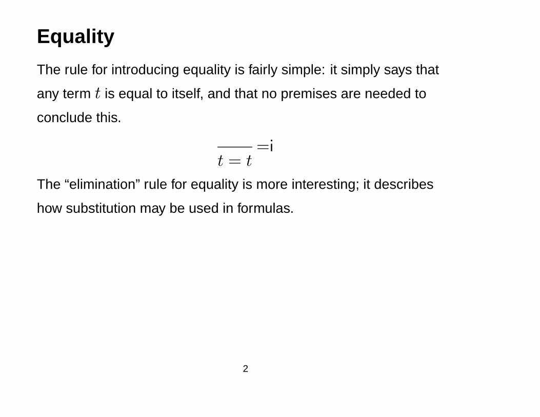
Equality

The rule for introducing equality is fairly simple: it simply says that

any term t is equal to itself, and that no premises are needed to

conclude this.

=it = t

The “elimination” rule for equality is more interesting; it describes

how substitution may be used in formulas.

2

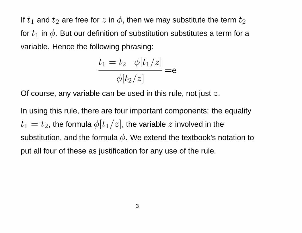
If t1 and t2 are free for z in φ, then we may substitute the term t2

for t1 in φ. But our definition of substitution substitutes a term for a

variable. Hence the following phrasing:

t1 = t2 φ[t1/z]=e

φ[t2/z]

Of course, any variable can be used in this rule, not just z.

In using this rule, there are four important components: the equality

t1 = t2, the formula φ[t1/z], the variable z involved in the

substitution, and the formula φ. We extend the textbook’s notation to

put all four of these as justification for any use of the rule.

3

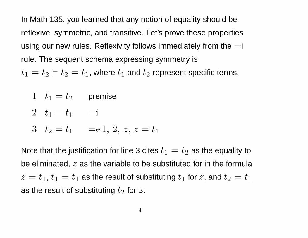
In Math 135, you learned that any notion of equality should be

reflexive, symmetric, and transitive. Let’s prove these properties

using our new rules. Reflexivity follows immediately from the =i

rule. The sequent schema expressing symmetry is

t1 = t2 ` t2 = t1, where t1 and t2 represent specific terms.

1 t1 = t2 premise

2 t1 = t1 =i

3 t2 = t1 =e 1, 2, z, z = t1

Note that the justification for line 3 cites t1 = t2 as the equality to

be eliminated, z as the variable to be substituted for in the formula

z = t1, t1 = t1 as the result of substituting t1 for z, and t2 = t1as the result of substituting t2 for z.

4

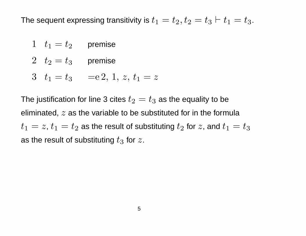
The sequent expressing transitivity is t1 = t2, t2 = t3 ` t1 = t3.

1 t1 = t2 premise

2 t2 = t3 premise

3 t1 = t3 =e 2, 1, z, t1 = z

The justification for line 3 cites t2 = t3 as the equality to be

eliminated, z as the variable to be substituted for in the formula

t1 = z, t1 = t2 as the result of substituting t2 for z, and t1 = t3

as the result of substituting t3 for z.

5

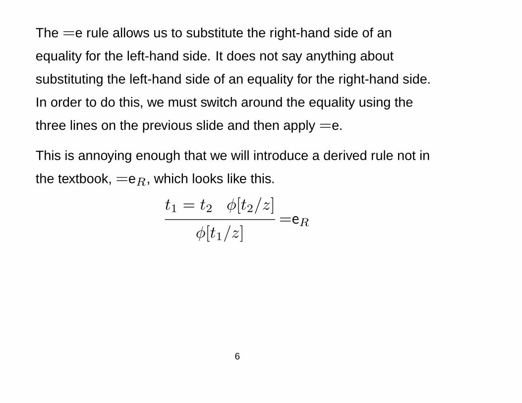
The =e rule allows us to substitute the right-hand side of an

equality for the left-hand side. It does not say anything about

substituting the left-hand side of an equality for the right-hand side.

In order to do this, we must switch around the equality using the

three lines on the previous slide and then apply =e.

This is annoying enough that we will introduce a derived rule not in

the textbook, =eR, which looks like this.

t1 = t2 φ[t2/z]=eR

φ[t1/z]

6

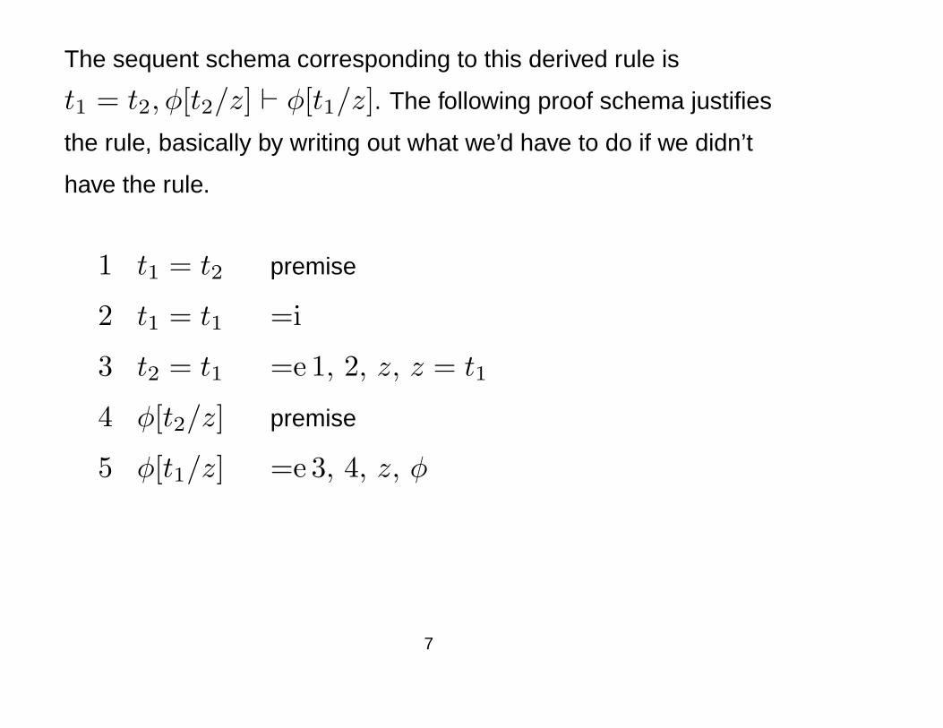
The sequent schema corresponding to this derived rule is

t1 = t2, φ[t2/z] ` φ[t1/z]. The following proof schema justifies

the rule, basically by writing out what we’d have to do if we didn’t

have the rule.

1 t1 = t2 premise

2 t1 = t1 =i

3 t2 = t1 =e 1, 2, z, z = t1

4 φ[t2/z] premise

5 φ[t1/z] =e 3, 4, z, φ

7

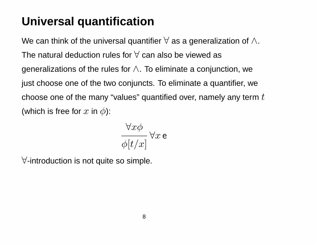
Universal quantification

We can think of the universal quantifier ∀ as a generalization of ∧.

The natural deduction rules for ∀ can also be viewed as

generalizations of the rules for ∧. To eliminate a conjunction, we

just choose one of the two conjuncts. To eliminate a quantifier, we

choose one of the many “values” quantified over, namely any term t

(which is free for x in φ):

∀xφ∀x e

φ[t/x]

∀-introduction is not quite so simple.

8

Recall that our rule for ∧-introduction was:

φ ψ∧i

φ ∧ ψThis suggests that to introduce a quantifier ∀x, we must prove the

formula being quantified for all possible “values”. This seems

impossible. Let’s look at a proof we did informally on the first day to

see how to proceed. We will phrase it slightly differently (but in a

fashion which will be familiar to you).

9

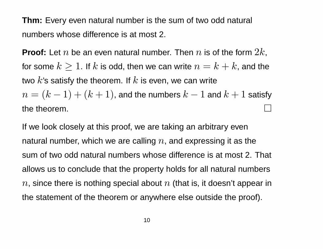
Thm: Every even natural number is the sum of two odd natural

numbers whose difference is at most 2.

Proof: Let n be an even natural number. Then n is of the form 2k,

for some k ≥ 1. If k is odd, then we can write n = k + k, and the

two k’s satisfy the theorem. If k is even, we can write

n = (k− 1) + (k+ 1), and the numbers k− 1 and k+ 1 satisfy

the theorem. �

If we look closely at this proof, we are taking an arbitrary even

natural number, which we are calling n, and expressing it as the

sum of two odd natural numbers whose difference is at most 2. That

allows us to conclude that the property holds for all natural numbers

n, since there is nothing special about n (that is, it doesn’t appear in

the statement of the theorem or anywhere else outside the proof).

10

This suggests that to prove a formula of the form ∀xφ, we can

prove φ with some arbitrary but fresh variable x0 substituted for x.

That is, we want to prove the formula φ[x0/x].

On the previous slide, we used n as a fresh variable, but in our

formal proofs, we adopt the convention of using subscripts (for

example, x0 as the fresh variable used to prove a ∀x statement).

The word “fresh” means that the variable has never been used

before in the proof. Furthermore, it will not be used once φ[x0/x]has been proved. It is “local” to this part of the proof. As we did with

assumptions, we enforce this locality by surrounding this part of the

proof with a proof box, putting the fresh variable as a label in the top

left corner.

11

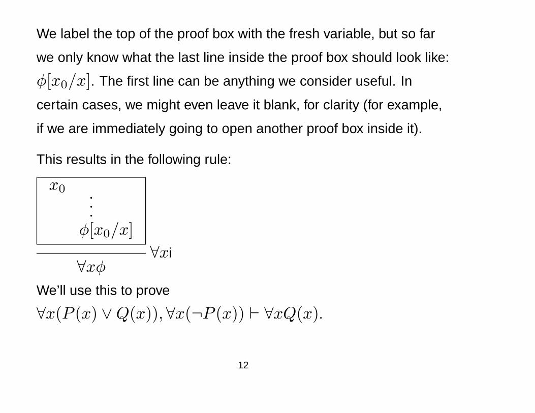
We label the top of the proof box with the fresh variable, but so far

we only know what the last line inside the proof box should look like:

φ[x0/x]. The first line can be anything we consider useful. In

certain cases, we might even leave it blank, for clarity (for example,

if we are immediately going to open another proof box inside it).

This results in the following rule:

x0 ···φ[x0/x]

∀xi∀xφ

We’ll use this to prove

∀x(P (x) ∨Q(x)),∀x(¬P (x)) ` ∀xQ(x).

12

1 ∀x(P (x) ∨Q(x)) premise

2 ∀x(¬P (x)) premise

x0 3 P (x0) ∨Q(x0) ∀xe 1

4 P (x0) assumption

5 ¬P (x0) ∀xe 2

6 ⊥ ¬e 4, 5

7 Q(x0) ⊥e 6

8 Q(x0) assumption

9 Q(x0) ∨e 3, 4− 7, 8

10 ∀xQ(x) ∀xi 3, 9

13

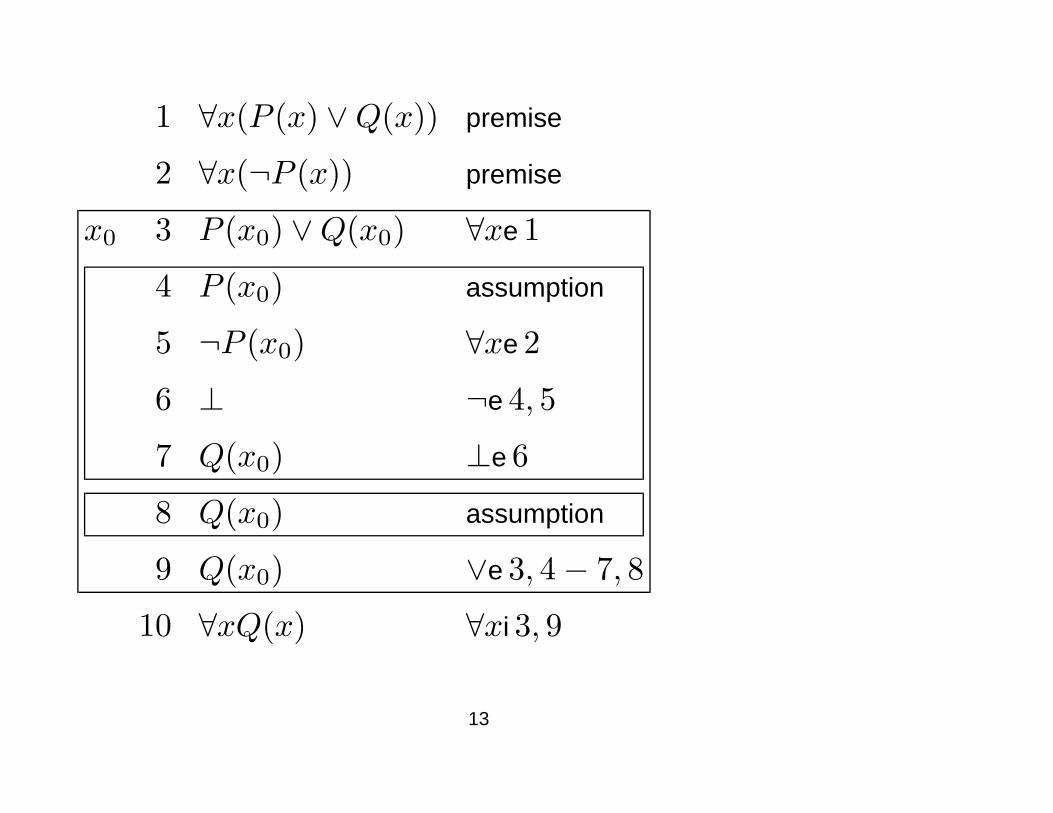
In the proof on the previous slide, we used ∀-elimination to create a

statement using the fresh variable, which appeared on the first line

of the proof box labelled with the fresh variable x0. We could also

have chosen to list a premise that did not mention the fresh variable,

or chosen to use some other rule, or left the first line blank.

Fresh variables are involved in one other proof rule to be discussed

shortly.

14

Existential quantification

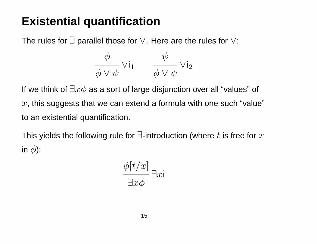
The rules for ∃ parallel those for ∨. Here are the rules for ∨:

φ∨i1

φ ∨ ψ

ψ∨i2

φ ∨ ψIf we think of ∃xφ as a sort of large disjunction over all “values” of

x, this suggests that we can extend a formula with one such “value”

to an existential quantification.

This yields the following rule for ∃-introduction (where t is free for x

in φ):

φ[t/x]∃xi

∃xφ

15

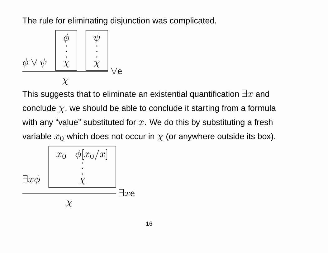
The rule for eliminating disjunction was complicated.

φ ∨ ψ

φ···χ

ψ···χ∨e

χ

This suggests that to eliminate an existential quantification ∃x and

conclude χ, we should be able to conclude it starting from a formula

with any “value” substituted for x. We do this by substituting a fresh

variable x0 which does not occur in χ (or anywhere outside its box).

∃xφ

x0 φ[x0/x]···χ

∃xeχ

16

To eliminate an existential quantification, we open a box and

introduce a fresh variable. Again, we use the convention that in

eliminating a formula of the form ∃xφ, our fresh variable should be

a subscripted version of x.

This rule dictates the first line of the box. The first line needs to be φ

with the fresh variable substituted for the quantified variable to be

eliminated; this line is labelled as an assumption. The last line

should be whatever statement we hope to take outside the box (as

is the case for the proof boxes used in or-elimination). That

statement cannot involve the fresh variable, as it is not permitted to

appear outside the proof box.

17

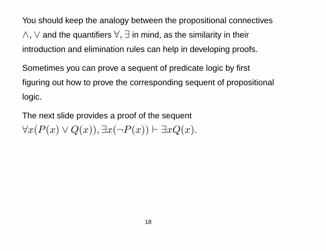
You should keep the analogy between the propositional connectives

∧,∨ and the quantifiers ∀,∃ in mind, as the similarity in their

introduction and elimination rules can help in developing proofs.

Sometimes you can prove a sequent of predicate logic by first

figuring out how to prove the corresponding sequent of propositional

logic.

The next slide provides a proof of the sequent

∀x(P (x) ∨Q(x)),∃x(¬P (x)) ` ∃xQ(x).

18

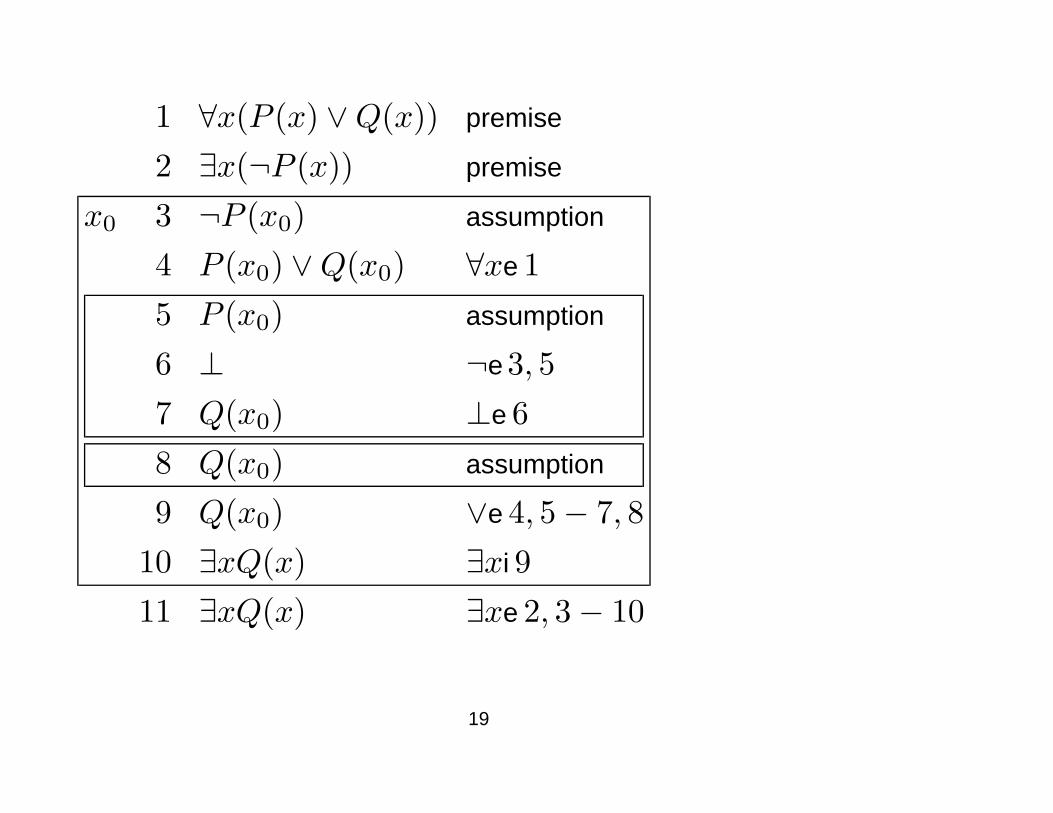
1 ∀x(P (x) ∨Q(x)) premise

2 ∃x(¬P (x)) premise

x0 3 ¬P (x0) assumption

4 P (x0) ∨Q(x0) ∀xe 15 P (x0) assumption

6 ⊥ ¬e 3, 57 Q(x0) ⊥e 68 Q(x0) assumption

9 Q(x0) ∨e 4, 5− 7, 810 ∃xQ(x) ∃xi 911 ∃xQ(x) ∃xe 2, 3− 10

19

Quantifier equivalences

Earlier we suggested that the statement “No students love CS 245”

had at least two possible translations, ¬∃x(S(x) ∧ L(x, c)) and

∀x(S(x)→ ¬L(x, c)), which we intuitively believed to be

semantically equivalent.

We should be able to prove the logical equivalence of these

formulas using our system of natural deduction. Theorem 2.13

(page 117) in the text covers a number of such equivalences. They

are grouped into four broad categories, and a representative proof is

presented for each one.

In lecture we will cover a couple of these proofs, leaving others to

reading, tutorial examples, or as exercises.

20

DeMorgan-style equivalences

These quantifier equivalences deal with moving negation from within

a quantifier to outside, or vice-versa. They are analogous to

DeMorgan’s laws for propositional logic.

Note that not all of these equivalences are intuitionistically valid.

The example we will prove is ∃x¬φ ` ¬∀xφ. This is a sequent

schema parameterized by an arbitrary formula φ, and as we did

before, we must present a proof schema which is not a formal proof

according to our rules, but becomes one for any specific φ.

The analogous propositional law is ¬p1 ∨ ¬p2 ` ¬(p1 ∧ p2), and

we prove this first to demonstrate the parallels.

21

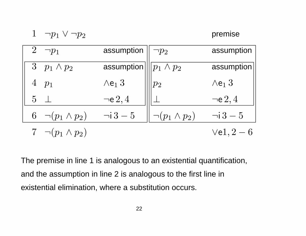
1 ¬p1 ∨ ¬p2 premise

2 ¬p1 assumption

3 p1 ∧ p2 assumption

4 p1 ∧e1 3

5 ⊥ ¬e 2, 4

6 ¬(p1 ∧ p2) ¬i 3− 5

¬p2 assumption

p1 ∧ p2 assumption

p2 ∧e1 3

⊥ ¬e 2, 4

¬(p1 ∧ p2) ¬i 3− 5

7 ¬(p1 ∧ p2) ∨e1, 2− 6

The premise in line 1 is analogous to an existential quantification,

and the assumption in line 2 is analogous to the first line in

existential elimination, where a substitution occurs.

22

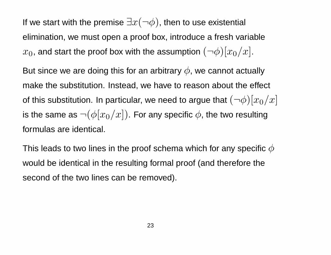
If we start with the premise ∃x(¬φ), then to use existential

elimination, we must open a proof box, introduce a fresh variable

x0, and start the proof box with the assumption (¬φ)[x0/x].

But since we are doing this for an arbitrary φ, we cannot actually

make the substitution. Instead, we have to reason about the effect

of this substitution. In particular, we need to argue that (¬φ)[x0/x]is the same as ¬(φ[x0/x]). For any specific φ, the two resulting

formulas are identical.

This leads to two lines in the proof schema which for any specific φ

would be identical in the resulting formal proof (and therefore the

second of the two lines can be removed).

23

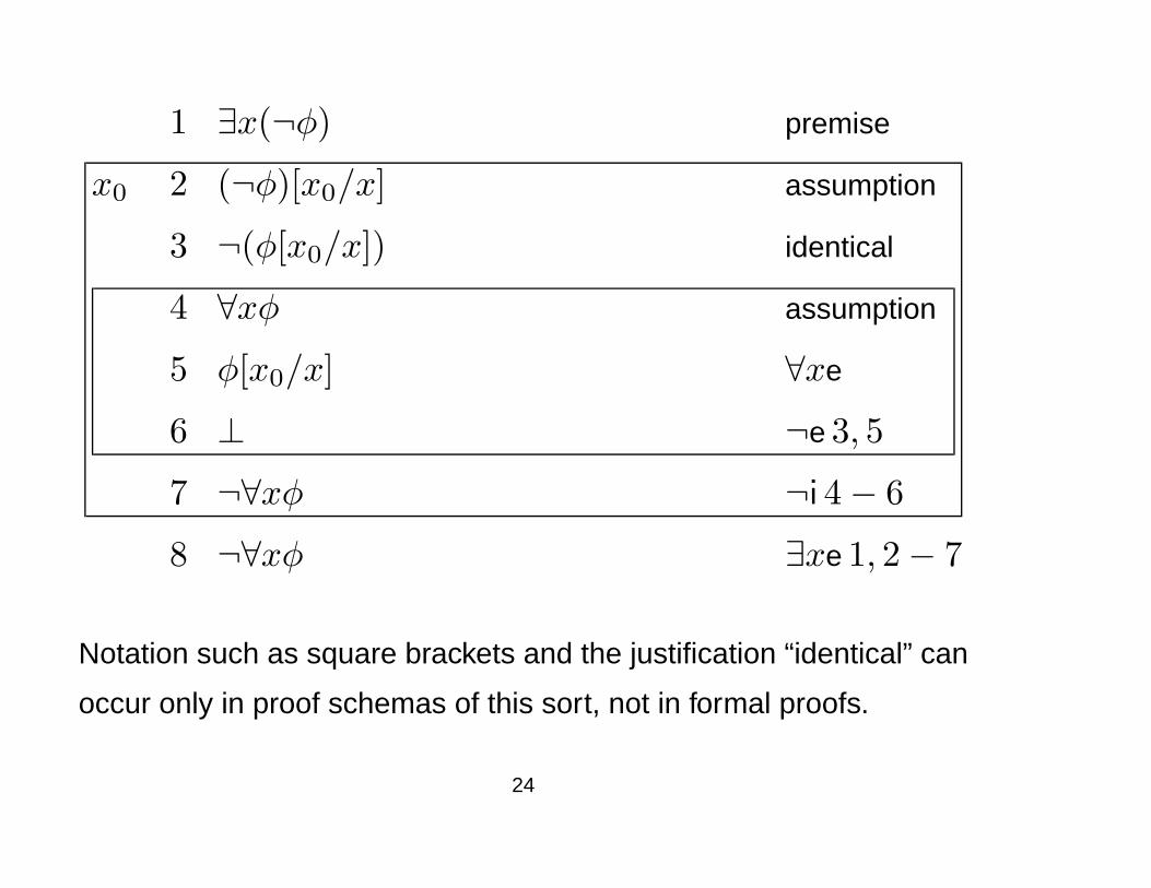
1 ∃x(¬φ) premise

x0 2 (¬φ)[x0/x] assumption

3 ¬(φ[x0/x]) identical

4 ∀xφ assumption

5 φ[x0/x] ∀xe

6 ⊥ ¬e 3, 5

7 ¬∀xφ ¬i 4− 6

8 ¬∀xφ ∃xe 1, 2− 7

Notation such as square brackets and the justification “identical” can

occur only in proof schemas of this sort, not in formal proofs.

24

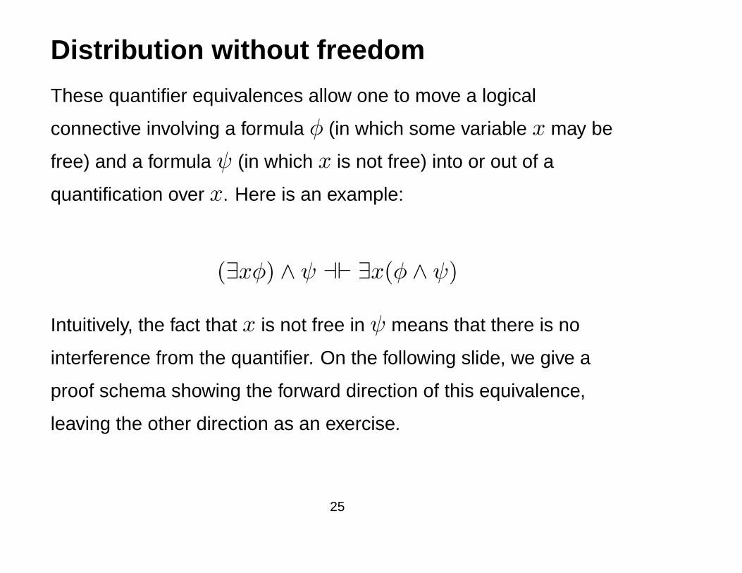
Distribution without freedom

These quantifier equivalences allow one to move a logical

connective involving a formula φ (in which some variable x may be

free) and a formula ψ (in which x is not free) into or out of a

quantification over x. Here is an example:

(∃xφ) ∧ ψ a` ∃x(φ ∧ ψ)

Intuitively, the fact that x is not free in ψ means that there is no

interference from the quantifier. On the following slide, we give a

proof schema showing the forward direction of this equivalence,

leaving the other direction as an exercise.

25

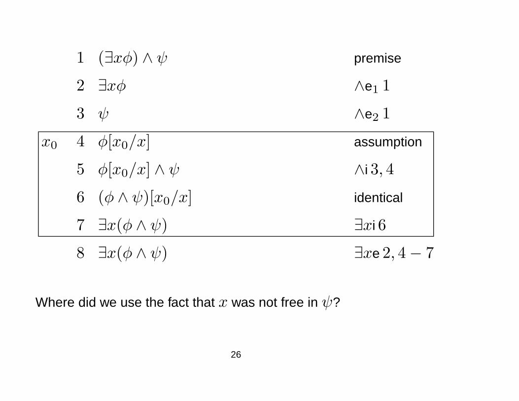
1 (∃xφ) ∧ ψ premise

2 ∃xφ ∧e1 1

3 ψ ∧e2 1

x0 4 φ[x0/x] assumption

5 φ[x0/x] ∧ ψ ∧i 3, 4

6 (φ ∧ ψ)[x0/x] identical

7 ∃x(φ ∧ ψ) ∃xi 6

8 ∃x(φ ∧ ψ) ∃xe 2, 4− 7

Where did we use the fact that x was not free in ψ?

26

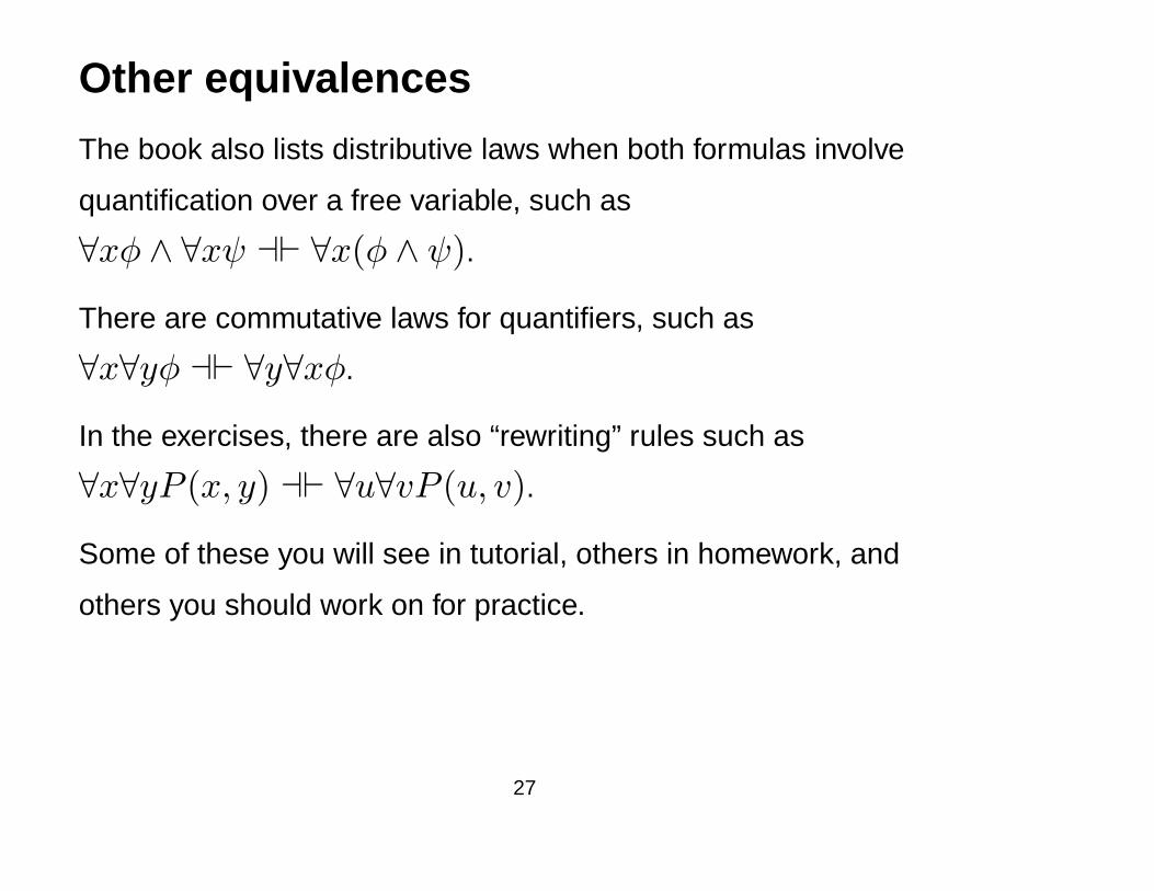
Other equivalences

The book also lists distributive laws when both formulas involve

quantification over a free variable, such as

∀xφ ∧ ∀xψ a` ∀x(φ ∧ ψ).

There are commutative laws for quantifiers, such as

∀x∀yφ a` ∀y∀xφ.

In the exercises, there are also “rewriting” rules such as

∀x∀yP (x, y) a` ∀u∀vP (u, v).

Some of these you will see in tutorial, others in homework, and

others you should work on for practice.

27

Intuitionism in predicate logic

The proof rules for =, ∀, and ∃ are all valid under intuitionism (the

latter two being generalizations of the rules for ∧ and ∨,

respectively).

The impact of intuitionist reasoning on predicate logic comes,

therefore, from the effect that the intuitionist perspective on negation

has on the kinds of proofs that can be derived.

As we have seen by now, intuitionist reasoning only allows for what

might be called “direct” proofs—a proof of φ�ψ must employ an

introduction rule for� (or the monkey’s uncle rule).

28

The impact of this observation in the context of propositional logic

was that whenever we arrive at the conclusion φ ∨ ψ, we always

have on hand either a proof of φ or a proof of ψ. In other words, we

always know which of φ or ψ is provable (or perhaps both are

provable).

Existential quantification is a generalization of disjunction. How

would an intuitionist read ∃xφ?

We have a proof that for some x0, φ[x0/x] holds?

OR

There is an x0 such that we have a proof of φ[x0/x]?

29

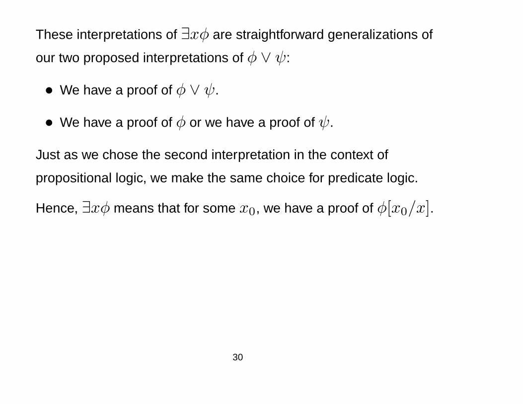
These interpretations of ∃xφ are straightforward generalizations of

our two proposed interpretations of φ ∨ ψ:

• We have a proof of φ ∨ ψ.

• We have a proof of φ or we have a proof of ψ.

Just as we chose the second interpretation in the context of

propositional logic, we make the same choice for predicate logic.

Hence, ∃xφ means that for some x0, we have a proof of φ[x0/x].

30

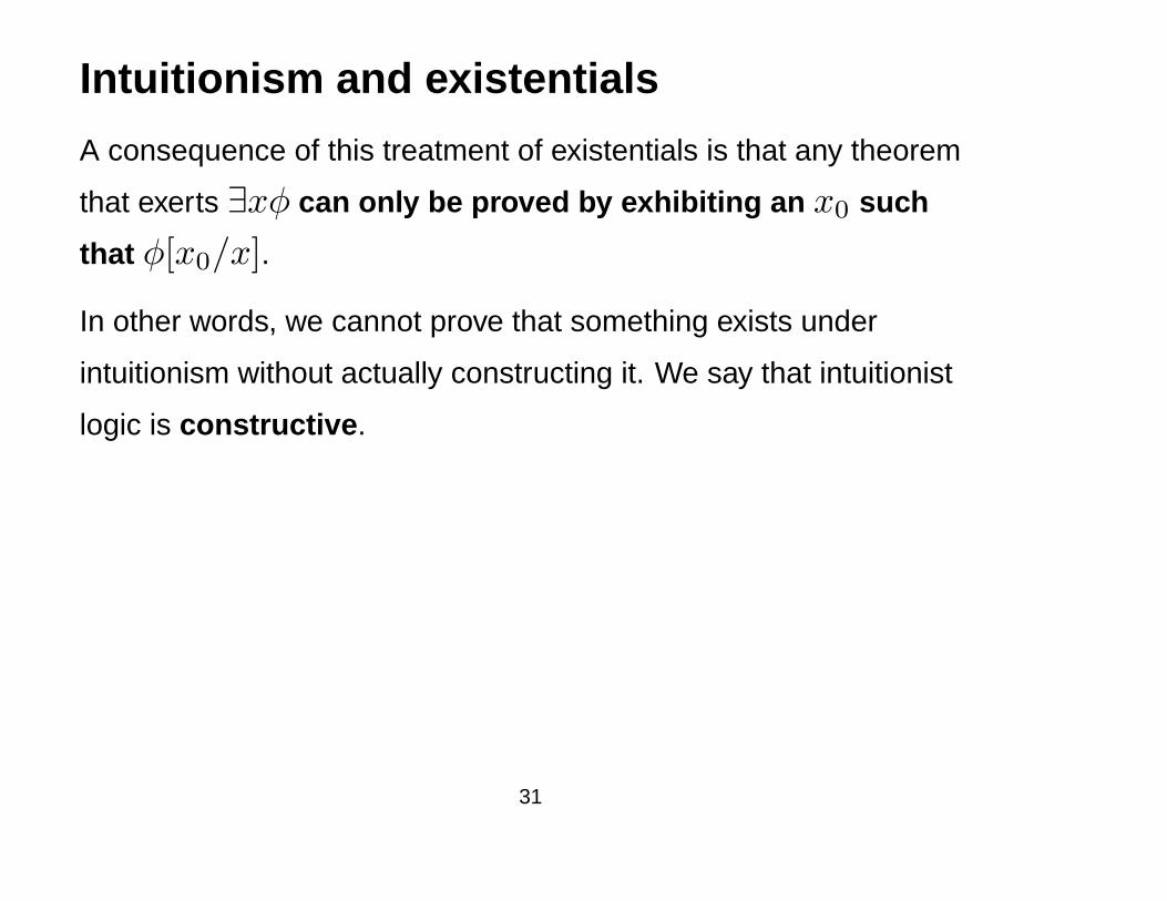
Intuitionism and existentials

A consequence of this treatment of existentials is that any theorem

that exerts ∃xφ can only be proved by exhibiting an x0 such

that φ[x0/x].

In other words, we cannot prove that something exists under

intuitionism without actually constructing it. We say that intuitionist

logic is constructive .

31

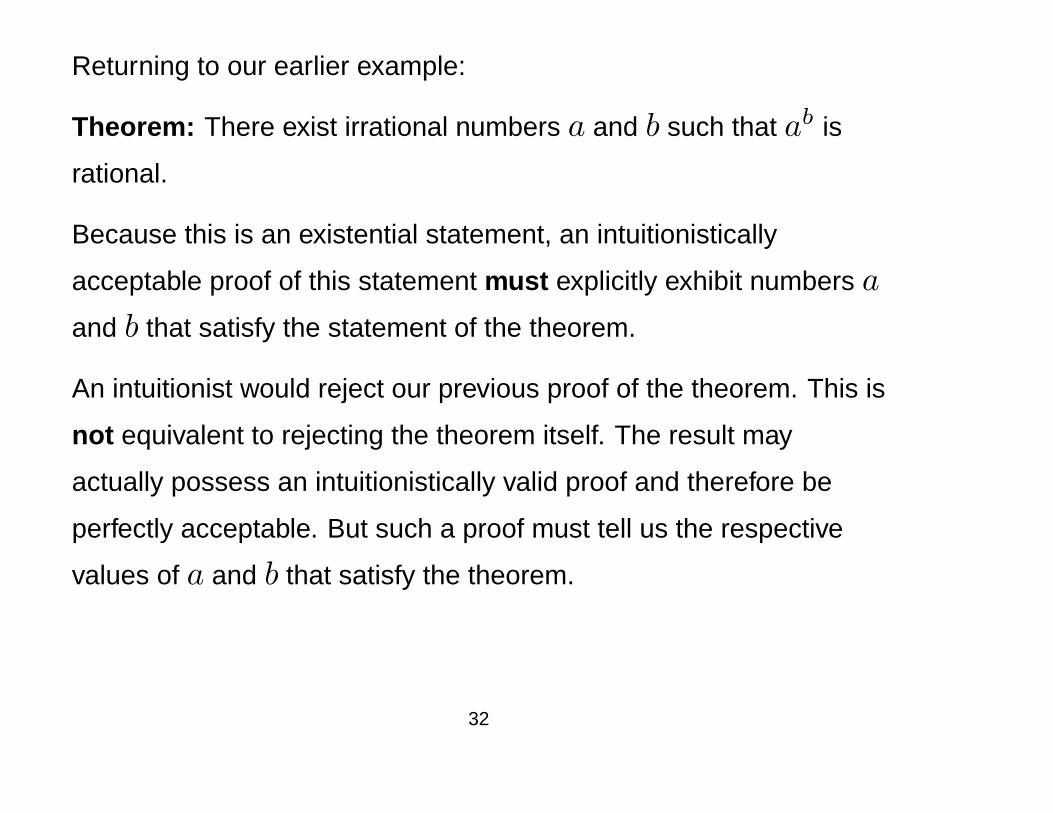
Returning to our earlier example:

Theorem: There exist irrational numbers a and b such that ab is

rational.

Because this is an existential statement, an intuitionistically

acceptable proof of this statement must explicitly exhibit numbers a

and b that satisfy the statement of the theorem.

An intuitionist would reject our previous proof of the theorem. This is

not equivalent to rejecting the theorem itself. The result may

actually possess an intuitionistically valid proof and therefore be

perfectly acceptable. But such a proof must tell us the respective

values of a and b that satisfy the theorem.

32

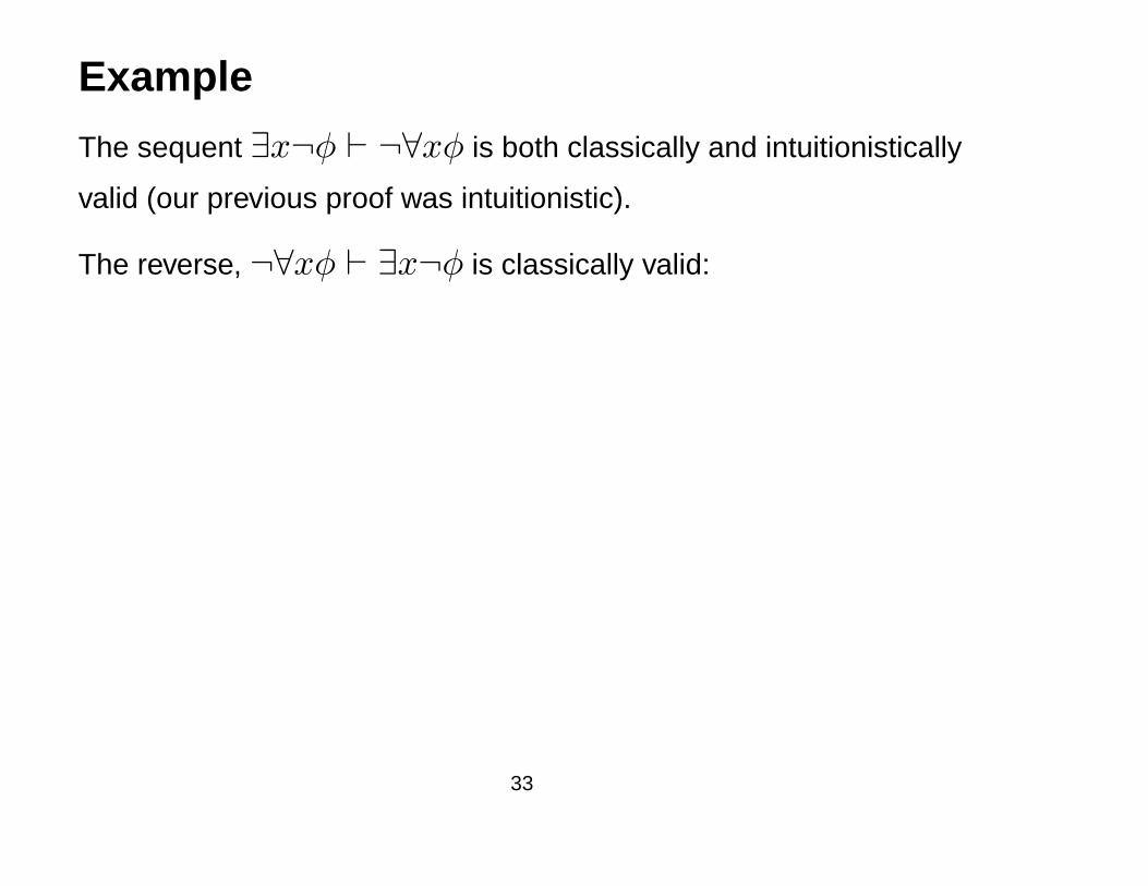
Example

The sequent ∃x¬φ ` ¬∀xφ is both classically and intuitionistically

valid (our previous proof was intuitionistic).

The reverse, ¬∀xφ ` ∃x¬φ is classically valid:

33

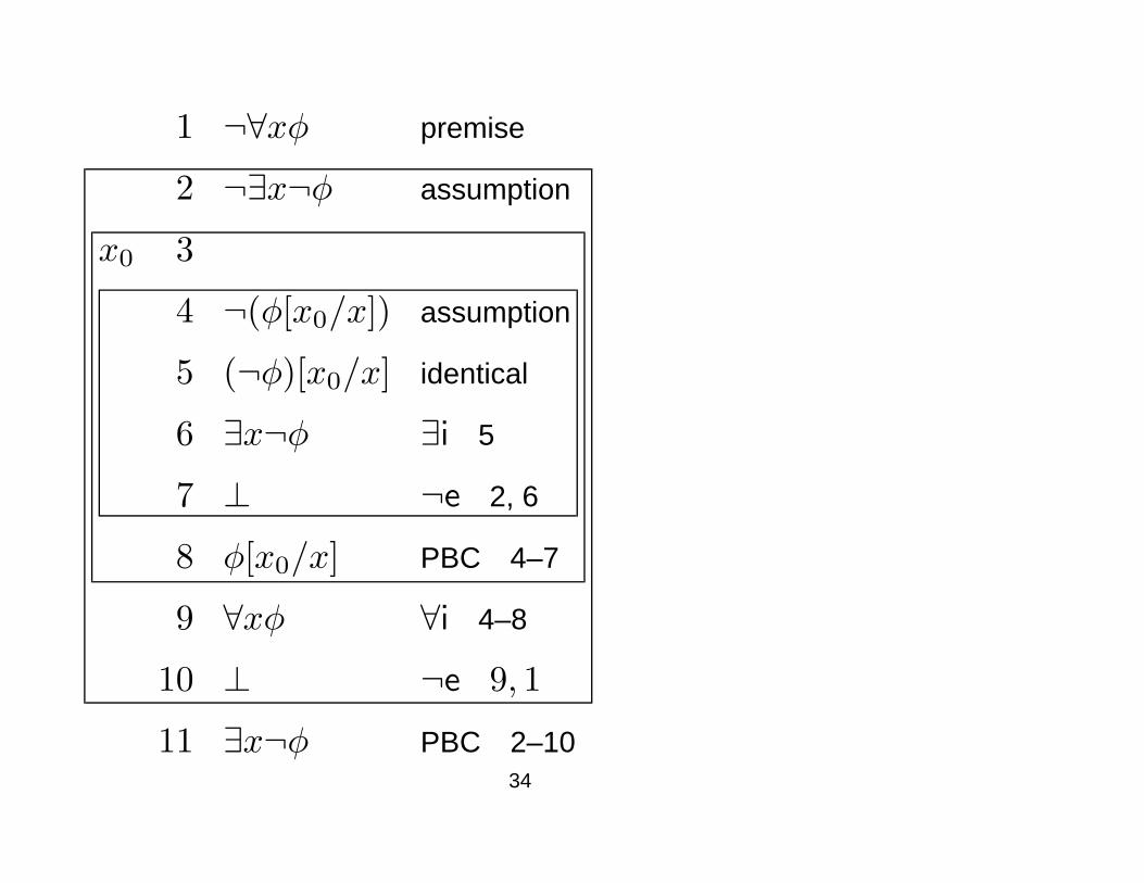
1 ¬∀xφ premise

2 ¬∃x¬φ assumption

x0 3

4 ¬(φ[x0/x]) assumption

5 (¬φ)[x0/x] identical

6 ∃x¬φ ∃i 5

7 ⊥ ¬e 2, 6

8 φ[x0/x] PBC 4–7

9 ∀xφ ∀i 4–8

10 ⊥ ¬e 9, 1

11 ∃x¬φ PBC 2–1034

On the other hand, we probably would not expect the sequent

¬∀xφ ` ∃x¬φ to hold under intuitionist logic.

Note: Rejecting a theorem is not the same as rejecting a proof. We

already know that the proof we just gave for ¬∀xφ ` ∃x¬φ is not

intuitionistically valid. That doesn’t mean that the theorem isn’t

intuitionistically valid—there might be an intuitionistic proof that we

haven’t found for it.

But for this example, we expect that the sequent is not

intuitionistically valid. The premise states that we cannot prove that

φ holds for every x. Since it is not clear from this statement how to

find a specific x0 such that φ[x0/x] is provably not provable, it

seems unlikely that we will find an intuitionist proof of ∃x¬φ, given

this premise.

35

The Drinker Paradox

The Drinker Paradox is an example of a classically valid theorem of

predicate logic that does not seem to match our intuition. Its

statement is as follows:

In any bar, there is a person such that if he or she drinks, then

everyone drinks. (Every bar has a “life of the party”?)

Let D be a unary predicate symbol, so that we might interpret

D(x) to mean “x drinks.”

Then the Drinker Paradox can be encoded as

∃x(D(x)→ ∀yD(y)) .

Perhaps not surprisingly, the paradox has no intuitionist proof.

36

What’s coming next?

In the next module, we will describe the semantics of predicate

logic, and discuss soundness and completeness without proof. Still

to come are other proof systems for predicate logic, and a

discussion of how to ensure that specific mathematical situations

(such as number theory or set theory) are properly formalized in

predicate logic.

To finish the course, we will look at a formal system for proving

programs (written in a very simple language) correct, and then

discuss software systems that uses ideas from predicate logic to try

to find counterexamples to specifications, as a form of debugging.

37

Goals of this module

You should add the six rules of natural deduction for equality and

quantifiers (plus the one derived rule we added) to the dozen-odd

rules for propositional logic that should already be in your head.

You should be able to use all of these rules to prove sequents for

predicate logic. Again, there are many exercises in the text that you

should look at, whether or not they are required on assignments,

because they reveal additional facets of the subject that we do not

have time to cover in lecture.

Make sure you are clear on the difference between rules of natural

deduction and quantifier equivalences. You can’t use a quantifier

equivalence to shorten a formal proof.

38