natural hazards, risk analysis and emergency preparedness
TRANSCRIPT
Louisiana State UniversityLSU Digital Commons
LSU Doctoral Dissertations Graduate School
2012
Natural Hazards, Risk Analysis and EmergencyPreparedness: Applying Spatial Methods inDisaster Risk Management APPLYING SPATIALMETHODS IN DISASTER RISKMANAGEMENTHenrike BrechtLouisiana State University and Agricultural and Mechanical College
Follow this and additional works at: https://digitalcommons.lsu.edu/gradschool_dissertations
Part of the Social and Behavioral Sciences Commons
This Dissertation is brought to you for free and open access by the Graduate School at LSU Digital Commons. It has been accepted for inclusion inLSU Doctoral Dissertations by an authorized graduate school editor of LSU Digital Commons. For more information, please [email protected].
Recommended CitationBrecht, Henrike, "Natural Hazards, Risk Analysis and Emergency Preparedness: Applying Spatial Methods in Disaster RiskManagement APPLYING SPATIAL METHODS IN DISASTER RISK MANAGEMENT" (2012). LSU Doctoral Dissertations. 2972.https://digitalcommons.lsu.edu/gradschool_dissertations/2972
NATURAL HAZARDS, RISK ANALYSIS AND EMERGENCY
PREPAREDNESS:
APPLYING SPATIAL METHODS IN DISASTER RISK MANAGEMENT
A Dissertation
Submitted to the Graduate Faculty of the
Louisiana State University and
Agricultural and Mechanical College
in partial fulfillment of the
Requirements for the degree of
Doctor of Philosophy
in
The Department of Geography and Anthropology
by
Henrike Brecht
M.S., Westfaelische Wilhelms-University Muenster, Germany, 2002
December 2012

ii
TABLE OF CONTENTS
LIST OF TABLES ................................................................................................................... IV
LIST OF FIGURES ................................................................................................................... V
ABSTRACT ........................................................................................................................... VII
CHAPTER 1 . INTRODUCTION .............................................................................................. 1
1.1 Setting the Stage ........................................................................................................... 1
1.2 The Problem .................................................................................................................. 5
1.2.1 Emergency Preparedness .................................................................................. 5
1.2.2 Risk Assessment ............................................................................................... 7
1.3 Dissertation Outline .................................................................................................... 10
1.4 References ................................................................................................................... 11
CHAPTER 2 . LOSING GROUND: HURRICANES AND THE RECEDING LOUISIANA
COASTLINE ............................................................................................................................ 13
2.1 Hurricanes ................................................................................................................... 14
2.2 Louisiana's Wetlands .................................................................................................. 21
2.3 The Barrier Islands as Louisiana's First Line of Defense ........................................... 24
2.4 Coastal Restoration Efforts ......................................................................................... 25
2.5 References ................................................................................................................... 27
CHAPTER 3 . THE APPLICATION OF GEOTECHNOLOGIES AFTER HURRICANE
KATRINA ................................................................................................................................ 30
3.1 Introduction ................................................................................................................. 30
3.2 Lessons Learned .......................................................................................................... 31
3.2.1 Managerial Lessons ..................................................................................... 322
3.2.2 Technology Infrastructure Lessons ............................................................... 34
3.2.3 Data Lessons .................................................................................................. 36
3.2.4 Operational Lessons and Workflows ............................................................. 39
3.2.5 Map Products ................................................................................................. 42
3.3 Conclusions ................................................................................................................. 44
3.4 References ................................................................................................................... 45
CHAPTER 4 . A GLOBAL URBAN RISK INDEX ............................................................... 47
4.1 Introduction ................................................................................................................. 47

iii
4.2 Background ................................................................................................................. 50
4.3 Motivation ................................................................................................................... 52
4.4 Methodology ............................................................................................................... 54
4.4.1 Assessing Hazards ......................................................................................... 55
4.4.2 Quantifying Exposure .................................................................................... 57
4.4.3 Calculating Vulnerability .............................................................................. 60
4.4.4 Determining Urban Risk ................................................................................ 63
4.4.5 Interpretation ................................................................................................. 65
4.5 Results ......................................................................................................................... 66
4.6 Sensitivity Analysis .................................................................................................... 78
4.7 Conclusion .................................................................................................................. 79
4.8 References ................................................................................................................... 80
CHAPTER 5 . SEA-LEVEL RISE AND STORM SURGES: HIGH STAKES FOR A
SMALL NUMBER OF COUNTRIES ..................................................................................... 84
5.1 Introduction ................................................................................................................. 84
5.2 Global Warming, Tropical Cyclone Intensity, and Disaster Preparedness ................. 87
5.3 Research Strategy and Data Sources ........................................................................... 89
5.4 Method ........................................................................................................................ 90
5.5 City Results ................................................................................................................. 95
5.5.1 Exposure of Coastal Area .............................................................................. 94
5.5.2 Exposure of Population ................................................................................. 96
5.6 Conclusions ................................................................................................................. 98
5.7 References ................................................................................................................. 100
CHAPTER 6 . CONCLUSION .............................................................................................. 105
6.1 Summary and Main Conclusions .............................................................................. 105
6.2 A Short Glance Ahead .............................................................................................. 108
APPENDIX 1 . GLOBAL URBAN RISK INDEX - CITY RANKING ............................... 112
APPENDIX 2 . COPYRIGHT PERMISSIONS .................................................................... 148
VITA ....................................................................................................................................... 155
iv
LIST OF TABLES
Table 4.1: Data sources for the hazard component .................................................................. 56
Table 4.2: Data sources for the exposure component ............................................................... 58
Table 4.3: Data sources for the vulnerability component ......................................................... 62
Table 4.4: The five most at risk countries for urban mortality and economic loss risk per
hazard ....................................................................................................................................... 69
Table 4.5: Regional top 5 cities most at risk to earthquakes .................................................... 71
Table 4.6: Regional top 5 cities most at risk to cyclones ......................................................... 72
Table 4.7: Regional top 5 cities most at risk to landslides ....................................................... 73
Table 4.8: Regional top 5 cities most at risk to floods ............................................................. 74
Table 5.1: Percent of national population in coastal cities, 1980 – 2000 ................................. 86
Table 5.2: Summary of data sources ........................................................................................ 90
Table 5.3: Exposure to future storm surge: Wave height increases of 10% and 15%.............. 95
Table 5.4: Top 25 City population exposure: Wave height increases of 10% and 15% .......... 97
Table 5.5: Projected national totals (‘000) for 2100: Coastal cities with populations greater
than 100,000 ............................................................................................................................. 99
v
LIST OF FIGURES
Figure 1.1: Number and type of disasters from 1980 to 2011 (Munich Re 2011) ..................... 1
Figure 1.2: Complementary nature of risk reduction and emergency preparedness .................. 6
Figure 1.3: Risk assessment methodology ................................................................................. 8
Figure 2.1: Distribution of hurricanes and tropical storms along the Louisiana coast from
1901 to 1996 (Stone et al 1997) ............................................................................................... 17
Figure 2.2: Tracks of hurricanes, tropical storms, and tropical disturbances to have made
landfall along or near the Louisiana coast from 1951-1996 (Stone et al. 1997) ...................... 19
Figure 2.3: More than 100 years of land change in south east Louisiana (1932-2050)
(adapted from USGS 2003) ...................................................................................................... 23
Figure 2.4: Chandeleurs Islands on July 17, 2001 and on August 31, 2005 (USGS 2005) ..... 25
Figure 2.5: Terraces encourage sediment deposition and protect existing wetlands by
reducing wave action in the shallow waters of Little Vermillion Bay, Louisiana (NOAA
2004) ......................................................................................................................................... 27
Figure 3.1: Illustration of the depth and extent of the inundation on August 31, 2005, caused
by Hurricane Katrina (NOAA 2005) ........................................................................................ 43
Figure 4.1: The four components of the Global Urban Risk Index .......................................... 54
Figure 4.2: Wind field of Hurricane Katrina in 2005 ............................................................... 57
Figure 4.3: Global cyclone frequency 1975-2007 .................................................................... 57
Figure 4.4: Integration of GRUMP data and Henderson Cities ............................................... 59
Figure 4.5: The six regions covered in the study ...................................................................... 63
Figure 4.6: Regional shares of urban risks for four different hazards ...................................... 68
Figure 4.7: Urban mortality risk .............................................................................................. 75
Figure 4.8: Urban economic loss risk ....................................................................................... 75

vi
Figure 4.9: 30 cities most at risk .............................................................................................. 76
Figure 4.10: Exposure to cyclones and earthquakes in large cities in 2000 and 2050 ............. 77
vii
ABSTRACT
Losses from natural hazards have been increasing steadily over the last decades. Yet,
tools exist that can reduce risks to disasters and prevent hazards from turning into disasters.
This study is intended to contribute to a reversal of the staggering economic losses by
advancing the application of Geographic Information Systems (GIS) in the field of disaster
risk management. Organized as a series of papers for publication, the dissertation first sets
the stage by presenting a case study on Louisiana and its vulnerability to hurricanes.
Thereafter, it examines and contributes to two fields that have proven to save lives and
lower damages following catastrophes: emergency preparedness and risk assessments.
Emergency preparedness, through contingency planning, disaster prediction, and
early warning, is critical to reduce disaster impacts. While GIS is increasingly recognized as
a key ingredient for successful emergency preparedness, systematic knowledge about how to
best use GIS is still in its infancy. This dissertation investigates the status quo of the use of
GIS in emergency preparedness and offers recommendations for moving ahead. Based on
interviews with emergency responders from three different U.S. states, the bottlenecks and
the successes of the use of GIS in the emergency response to Hurricane Katrina are
examined.
Risk assessments are tools to identify and understand risk. Given the high loss
potential in urban areas, surprisingly little is known about the risk of cities. Oddly, a
comprehensive ranking of cities’ risk has been lacking. This research addresses this gap by
developing, for the first time, a disaster risk ranking of the world’s major cities. The ranking
measures mortality and economic risks to major natural hazards for the 1,943 main cities in
110 countries. Building on these efforts, the most recent scientific and demographic

viii
information is applied in order to estimate the future impacts of climate change on storm
surges that will strike coastal urban populations.

1
CHAPTER 1 : INTRODUCTION
INTRODUCTION
1.1 Setting the Stage
Economic losses from natural hazards have been rising steadily in the past few
decades (Figure 1.1). For example, in the period between 1990 and 1999, the costs of
disasters, in constant dollars, were more than 15 times higher than during the period 1950-59
(World Bank 2006). The year of 2011 has been no exception to this trend and was the
costliest year on record for disasters. Economic losses in 2011 amounted to US$380 billion,
far exceeding the previous record set in 2005 (US$220 billion) (Munich Re 2012).
Figure 1.1: Number and type of disasters from 1980 to 2011 (Munich Re 2011)
2
The main reason for this upward trend is an increased concentration of individuals and
assets in hazard prone areas. The world’s population and economic activity have become
concentrated in vulnerable locations near earthquake faults, on subsiding river deltas, and
along tropical coastal zones. The proportion of the global population living in flood-prone
river basins has increased by 114% while those living on cyclone exposed coastlines have
grown by 192% over the past 30 years (ISDR 2011). The risks will continue to rise over the
next decades as trillions of dollars flow into new public investments in vulnerable areas and as
the wealth in flood-prone Manila or earthquake-prone Bogota increases.
Multi-billion-dollar disasters have become more widespread. The 2011 Great Eastern
Japanese Earthquake, the 2011 Thai floods, the 2010 Pakistan flooding, and the 2010 Haiti
earthquake are some of the most devastating natural hazards on record. Especially developing
countries are suffering with more than 95% of disaster deaths occurring in the developing
world in the past 25 years (Arnold & Kreimer 2004) and with economic losses being 20 times
greater (as a percentage of GDP) than in the developed world (World Bank 2006).
These loss trends may sound gloomy but with the right policies and technical
measures, these loss trends can be reversed. Increasing exposure does not necessarily mean
increasing disaster risk. In the last two decades, risk reduction efforts have succeeded in
reducing the death toll of natural hazards, despite the world’s growing population, through
improved early warning, more stringent building codes, and better contingency planning.
Economic costs from disasters, however, have risen relentlessly due to the accumulation of
wealth in vulnerable areas. Yet, while natural hazards are inevitable, options exist to ensure
that they do not become disasters. A range of disaster risk management activities and smart
3
solutions with high cost-benefit ratios exists. These activities and solutions help reduce human
and also economic vulnerability to disasters.
Disaster risk management
Disaster Risk Management (DRM) is a set of tools, used to identify, reduce, prepare
for, and recover from disasters. Disaster risk management is commonly organized into five
main components (e.g., Ghesquiere and Mahul 2010):
Risk assessments provide information on severity, frequency, geographical extent and
causes of disasters and give individuals the necessary knowledge to make informed
decisions about risk reduction measures.
Risk reduction consists of a blend of hard measures and soft measures. The former
include flood control reservoirs, levees, hurricane shutters, and earthquake resilient
beams. The latter include institutional arrangements, land use regulation, education, and
provision of economic incentives.
Financial protection through insurance and risk transfer reduces the financial challenges
of governments in the aftermath of disasters while protecting the long-term fiscal balance.
Emergency preparedness reduces residual risks and includes contingency planning,
early warning systems, and crisis management institutions as well as instruments.
Recovery and reconstruction in a post-disaster environment often presents a window of
opportunity to rebuild smarter and to mainstream resilience into reconstruction policies.
This dissertation focuses on two of the five components in the realm of disaster risk
management; namely on risk assessments and emergency preparedness. It is the aim of the
4
research presented here to enhance the complementary nature of Geographic Information
System (GIS) and disaster risk management, which are two disciplines that benefit from
further realizing each other’s potential. In the area of risk assessments, the thesis presents and
analyzes urban risk and thereby aims to raise public awareness and give reference points for
investment decisions. In the area of emergency preparedness, the dissertation seeks to
advance an improved use of GIS in order to efficiently prepare for, and respond to, disasters.
The Application of Geographic Information Systems in Disaster Risk Management
GIS technology is a tool for understanding vulnerabilities and prioritizing mitigation
efforts to reduce the impact of future disasters. It can effectively catalyze the processes of the
five DRM components since all of them benefit from access to, and analysis of, complex
spatial analysis and maps. The convergence of the two fields of GIS and DRM has increased
gradually over the last two decades. In the 1990s, much of the research that integrated GIS
and hazard studies was restricted to producing cartographic products rather than spatial
modeling. Since 2000, however, the use of GIS has evolved from mapping tools to modeling
and simulation instruments. In the last few years, with increasing internet connectivity, mobile
phone use, and user-generated content, crowdsourcing has emerged as a dynamic and open
way to visualize and map risks and disasters. For example, crisis mapping has been successful
in making use of mobile and web-based applications, crowdsourced event data, and satellite
imagery to support early warning and rapid response. Nevertheless, significant gaps in using
the full GIS potential in disaster risk management remain as this dissertation shows.
5
1.2 The Problem
1.2.1 Emergency Preparedness
Definition
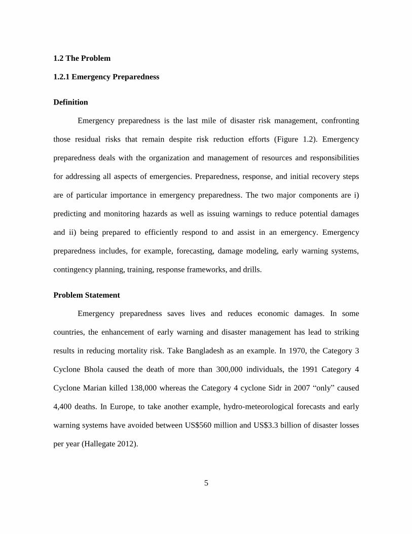
Emergency preparedness is the last mile of disaster risk management, confronting
those residual risks that remain despite risk reduction efforts (Figure 1.2). Emergency
preparedness deals with the organization and management of resources and responsibilities
for addressing all aspects of emergencies. Preparedness, response, and initial recovery steps
are of particular importance in emergency preparedness. The two major components are i)
predicting and monitoring hazards as well as issuing warnings to reduce potential damages
and ii) being prepared to efficiently respond to and assist in an emergency. Emergency
preparedness includes, for example, forecasting, damage modeling, early warning systems,
contingency planning, training, response frameworks, and drills.
Problem Statement
Emergency preparedness saves lives and reduces economic damages. In some
countries, the enhancement of early warning and disaster management has lead to striking
results in reducing mortality risk. Take Bangladesh as an example. In 1970, the Category 3
Cyclone Bhola caused the death of more than 300,000 individuals, the 1991 Category 4
Cyclone Marian killed 138,000 whereas the Category 4 cyclone Sidr in 2007 “only” caused
4,400 deaths. In Europe, to take another example, hydro-meteorological forecasts and early
warning systems have avoided between US$560 million and US$3.3 billion of disaster losses
per year (Hallegate 2012).
6
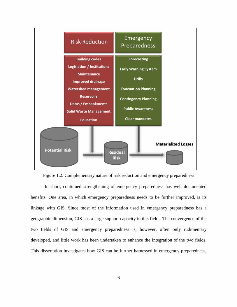
Figure 1.2: Complementary nature of risk reduction and emergency preparedness
In short, continued strengthening of emergency preparedness has well documented
benefits. One area, in which emergency preparedness needs to be further improved, is its
linkage with GIS. Since most of the information used in emergency preparedness has a
geographic dimension, GIS has a large support capacity in this field. The convergence of the
two fields of GIS and emergency preparedness is, however, often only rudimentary
developed, and little work has been undertaken to enhance the integration of the two fields.
This dissertation investigates how GIS can be further harnessed in emergency preparedness,
Building codes
Legislation / Institutions
Maintenance
Improved drainage
Watershed management
Reservoirs
Dams / Embankments
Solid Waste Management
Education
Forecasting
Early Warning System
Drills
Evacuation Planning
Contingency Planning
Public Awareness
Clear mandates
Risk Reduction Emergency
Preparedness
Residual Risk
Reduced Risk
Materialized Losses Potential Risk

7
specifically in the two areas of hurricane forecasts and disaster management. In particular, this
dissertation poses the following question:
How can the application of GIS be improved in the emergency response phase?
Objectives
The research presented herein aims at finding methods that enhance the convergence
of the two fields of GIS and emergency preparedness. To achieve this goal, a main research
objective has been formed:
Use interviews with GIS emergency responders to analyze the bottlenecks and good
practices of the use of GIS in response to Hurricane Katrina and to draw
conclusions for enhancing preparedness.
1.2.2 Risk Assessment
Definition
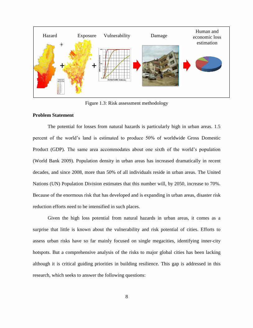
A risk assessment is a method to determine the nature and extent of risks by analyzing
hazards, vulnerability, and the extent of human and asset exposure (Figure 1.3). It provides
information on severity, frequency, geographical extent, and causes of disasters. This
information enables informed decision-making with respect to how risk should be managed
and which measures to implement. Quantifying risk and expected future losses is not only the
first step in a disaster risk reduction program. The outputs and scenarios of a risk assessment
also contribute to the structuring of an overall development project. The Hyogo Framework
for Action 2005-2015 (ISDR 2005), signed by 186 nations, characterizes risk assessments as a
central activity in defining priorities and building resilience.
8
Hazard Exposure Vulnerability Damage
Figure 1.3: Risk assessment methodology
Problem Statement
The potential for losses from natural hazards is particularly high in urban areas. 1.5
percent of the world’s land is estimated to produce 50% of worldwide Gross Domestic
Product (GDP). The same area accommodates about one sixth of the world’s population
(World Bank 2009). Population density in urban areas has increased dramatically in recent
decades, and since 2008, more than 50% of all individuals reside in urban areas. The United
Nations (UN) Population Division estimates that this number will, by 2050, increase to 70%.
Because of the enormous risk that has developed and is expanding in urban areas, disaster risk
reduction efforts need to be intensified in such places.
Given the high loss potential from natural hazards in urban areas, it comes as a
surprise that little is known about the vulnerability and risk potential of cities. Efforts to
assess urban risks have so far mainly focused on single megacities, identifying inner-city
hotspots. But a comprehensive analysis of the risks to major global cities has been lacking
although it is critical guiding priorities in building resilience. This gap is addressed in this
research, which seeks to answer the following questions:
+ +
Human and
economic loss
estimation
9
Which cities are likely to be affected by a disaster?
In which cities is the risk of mortality due to natural hazards the highest?
Which cities are most at risk of economic losses due to natural hazards?
Which cities will be highly impacted by climate change and storm surges?
The study will enhance the knowledge of the variation of urban risks. Such knowledge
is useful for local and national planners, as well as international donors. Disclosing risks to
cities raises awareness, informs the prioritization of resources, inspires further research,
particularly at local levels, and promotes a shift towards managing risks rather than
emergencies.
Objective
The goal of this study is to present, for the first time, a risk ranking of the world’s
major cities in 110 less developed countries. I chose to mask out the developed countries in
this study since the main intended audience are multilateral and bilateral development
institutions, which, in past have often expressed the need for such as study in order to better
allocate official development assistance (ODA) funding for disaster risk management where it
is most needed. The risks from the four most common types of natural hazards are evaluated
for nearly 2,000 cities. The fields of disaster risk management and climate change adaptation
have a significant overlap of concepts and shared goals and should therefore be addressed in a
joint manner, otherwise policy incoherence, ineffective use of resources, and duplication of
efforts can easily occur. I therefore included climate change in the risk assessment by
analyzing the impacts of sea level risk and future storm surges on cities. Three fundamental
research objectives were established:
10
Apply global spatial data layers for the four modules: hazard, exposure, vulnerability,
and losses. This is done in order to assess the urban risks in all major cities of the less
developed world from four different natural hazards: earthquakes, landslides, floods,
and cyclones.
Present the results in the form of an urban index that allows for the comparison of risk
levels worldwide in a self-explanatory manner and that gives reference points for local
and national planners as well as international donors for investment decisions.
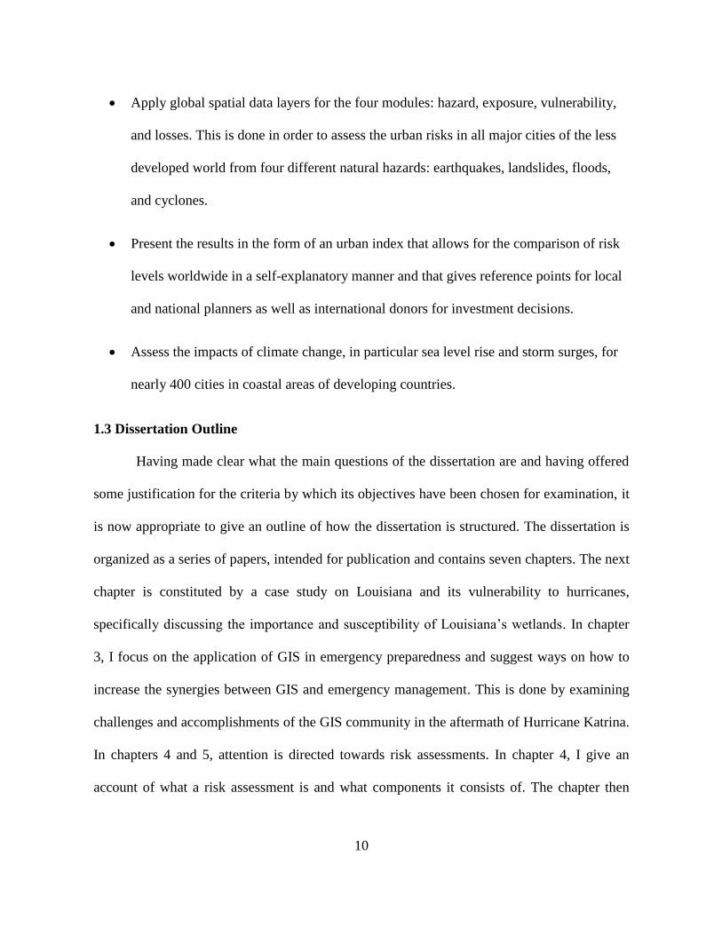
Assess the impacts of climate change, in particular sea level rise and storm surges, for
nearly 400 cities in coastal areas of developing countries.
1.3 Dissertation Outline
Having made clear what the main questions of the dissertation are and having offered
some justification for the criteria by which its objectives have been chosen for examination, it
is now appropriate to give an outline of how the dissertation is structured. The dissertation is
organized as a series of papers, intended for publication and contains seven chapters. The next
chapter is constituted by a case study on Louisiana and its vulnerability to hurricanes,
specifically discussing the importance and susceptibility of Louisiana’s wetlands. In chapter
3, I focus on the application of GIS in emergency preparedness and suggest ways on how to
increase the synergies between GIS and emergency management. This is done by examining
challenges and accomplishments of the GIS community in the aftermath of Hurricane Katrina.
In chapters 4 and 5, attention is directed towards risk assessments. In chapter 4, I give an
account of what a risk assessment is and what components it consists of. The chapter then
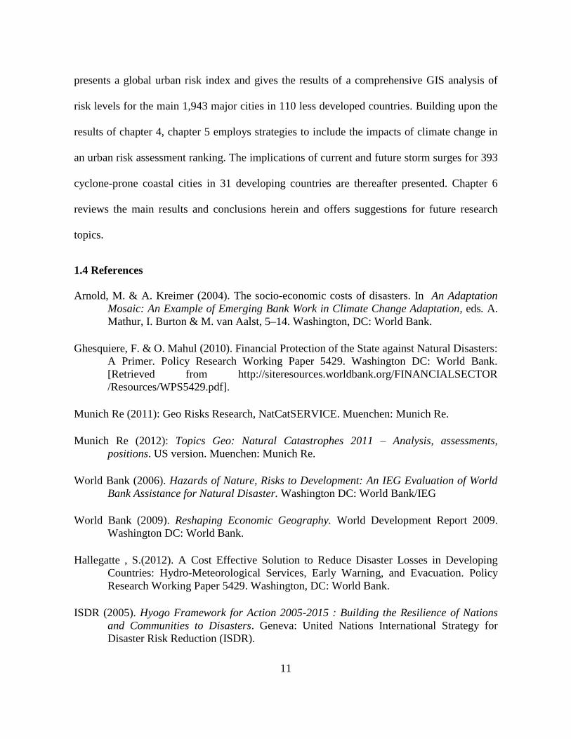
11
presents a global urban risk index and gives the results of a comprehensive GIS analysis of
risk levels for the main 1,943 major cities in 110 less developed countries. Building upon the
results of chapter 4, chapter 5 employs strategies to include the impacts of climate change in
an urban risk assessment ranking. The implications of current and future storm surges for 393
cyclone-prone coastal cities in 31 developing countries are thereafter presented. Chapter 6
reviews the main results and conclusions herein and offers suggestions for future research
topics.
1.4 References
Arnold, M. & A. Kreimer (2004). The socio-economic costs of disasters. In An Adaptation
Mosaic: An Example of Emerging Bank Work in Climate Change Adaptation, eds. A.
Mathur, I. Burton & M. van Aalst, 5–14. Washington, DC: World Bank.
Ghesquiere, F. & O. Mahul (2010). Financial Protection of the State against Natural Disasters:
A Primer. Policy Research Working Paper 5429. Washington DC: World Bank.
[Retrieved from http://siteresources.worldbank.org/FINANCIALSECTOR
/Resources/WPS5429.pdf].
Munich Re (2011): Geo Risks Research, NatCatSERVICE. Muenchen: Munich Re.
Munich Re (2012): Topics Geo: Natural Catastrophes 2011 – Analysis, assessments,
positions. US version. Muenchen: Munich Re.
World Bank (2006). Hazards of Nature, Risks to Development: An IEG Evaluation of World
Bank Assistance for Natural Disaster. Washington DC: World Bank/IEG
World Bank (2009). Reshaping Economic Geography. World Development Report 2009.
Washington DC: World Bank.
Hallegatte , S.(2012). A Cost Effective Solution to Reduce Disaster Losses in Developing
Countries: Hydro-Meteorological Services, Early Warning, and Evacuation. Policy
Research Working Paper 5429. Washington, DC: World Bank.
ISDR (2005). Hyogo Framework for Action 2005-2015 : Building the Resilience of Nations
and Communities to Disasters. Geneva: United Nations International Strategy for
Disaster Risk Reduction (ISDR).

12
ISDR (2011). Global Assessment Report on Disaster Risk Reduction 2011: Revealing Risk,
Redefining Development. Geneva: United Nations International Strategy for Disaster
Risk Reduction (ISDR).
13
CHAPTER 2 : LOSING GROUND: HURRICANES AND THE RECEDING
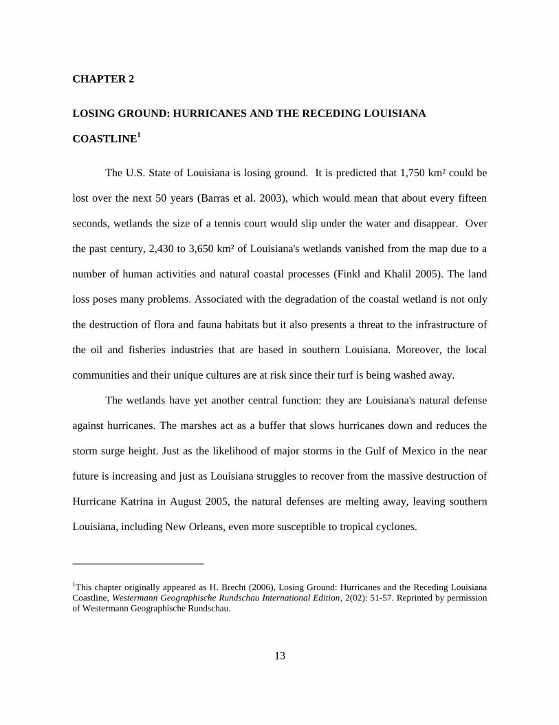
LOSING GROUND: HURRICANES AND THE RECEDING LOUISIANA
COASTLINE1
The U.S. State of Louisiana is losing ground. It is predicted that 1,750 km² could be
lost over the next 50 years (Barras et al. 2003), which would mean that about every fifteen
seconds, wetlands the size of a tennis court would slip under the water and disappear. Over
the past century, 2,430 to 3,650 km² of Louisiana's wetlands vanished from the map due to a
number of human activities and natural coastal processes (Finkl and Khalil 2005). The land
loss poses many problems. Associated with the degradation of the coastal wetland is not only
the destruction of flora and fauna habitats but it also presents a threat to the infrastructure of
the oil and fisheries industries that are based in southern Louisiana. Moreover, the local
communities and their unique cultures are at risk since their turf is being washed away.
The wetlands have yet another central function: they are Louisiana's natural defense
against hurricanes. The marshes act as a buffer that slows hurricanes down and reduces the
storm surge height. Just as the likelihood of major storms in the Gulf of Mexico in the near
future is increasing and just as Louisiana struggles to recover from the massive destruction of
Hurricane Katrina in August 2005, the natural defenses are melting away, leaving southern
Louisiana, including New Orleans, even more susceptible to tropical cyclones.
1This chapter originally appeared as H. Brecht (2006), Losing Ground: Hurricanes and the Receding Louisiana
Coastline, Westermann Geographische Rundschau International Edition, 2(02): 51-57. Reprinted by permission
of Westermann Geographische Rundschau.
14
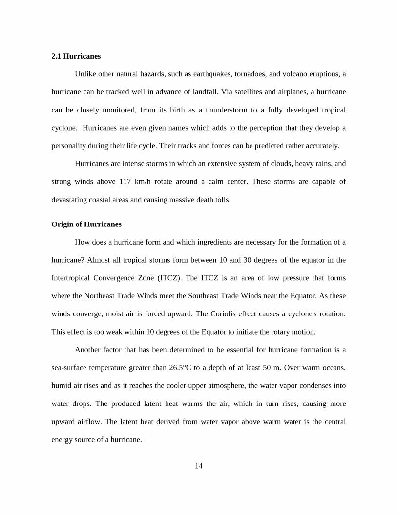
2.1 Hurricanes
Unlike other natural hazards, such as earthquakes, tornadoes, and volcano eruptions, a
hurricane can be tracked well in advance of landfall. Via satellites and airplanes, a hurricane
can be closely monitored, from its birth as a thunderstorm to a fully developed tropical
cyclone. Hurricanes are even given names which adds to the perception that they develop a
personality during their life cycle. Their tracks and forces can be predicted rather accurately.
Hurricanes are intense storms in which an extensive system of clouds, heavy rains, and
strong winds above 117 km/h rotate around a calm center. These storms are capable of
devastating coastal areas and causing massive death tolls.
Origin of Hurricanes
How does a hurricane form and which ingredients are necessary for the formation of a
hurricane? Almost all tropical storms form between 10 and 30 degrees of the equator in the
Intertropical Convergence Zone (ITCZ). The ITCZ is an area of low pressure that forms
where the Northeast Trade Winds meet the Southeast Trade Winds near the Equator. As these
winds converge, moist air is forced upward. The Coriolis effect causes a cyclone's rotation.
This effect is too weak within 10 degrees of the Equator to initiate the rotary motion.
Another factor that has been determined to be essential for hurricane formation is a
sea-surface temperature greater than 26.5°C to a depth of at least 50 m. Over warm oceans,
humid air rises and as it reaches the cooler upper atmosphere, the water vapor condenses into
water drops. The produced latent heat warms the air, which in turn rises, causing more
upward airflow. The latent heat derived from water vapor above warm water is the central
energy source of a hurricane.
15
Other circumstances for hurricane development include quickly decreasing
temperatures in the upper atmosphere and high humidity in the troposphere. The high
humidity reduces the amount of evaporation in clouds and maximizes the latent heat to be
released. Apart from that, a low wind shear, i.e. relative homogenous wind direction and
strength at different levels of the atmosphere, contributes to cyclone development. Finally, a
trigger for convergence must be present, for example in the form of an easterly wave, which is
a westward moving area of convergent winds. Other triggers are a weak frontal boundary and
tropical upper tropospheric troughs, both of which produce deep convection.
Life Cycle of a Hurricane
Stage 1 - Tropical Wave: A tropical wave is the birth stage of a hurricane. It has only a
slight circulation without closed isobars around a small pressure drop. The wind speeds are
less than 40 km/h. These tropical disturbances originate regularly in the intertropical
convergence zone and are often accompanied by thunderstorms, cloudiness, and precipitation.
Stage 2 - Tropical Depression: A disturbance is upgraded to a tropical depression
when a number of thunderstorms cluster together and an organized circulation in the center of
the thunderstorm complex occurs. This circulation is characterized by a wind speed below 65
km/h near the center and by at least one closed isobar that accompanies a lower pressure in
the storm center. Tropical depressions are not named but numbered (no. 1, no. 2, etc.).
Stage 3 - Tropical Storm: When a tropical depression intensifies and the maximum
sustained winds are between 65 km/h and 115 km/h, it becomes a tropical storm and is
assigned a name. Tropical storms are more organized than depressions and they have an
16
intensified circulation. These storms can cause extensive damage even without becoming a
hurricane. Slow-moving tropical storms can drop torrential rainfall.
Stage 4 – Hurricane: A tropical storm becomes a hurricane when sustained wind
speeds are at least 119 km/h. A pronounced circulation develops around the hurricane eye, an
area of relative calm and low atmospheric pressure. The wall that surrounds the eye is about
15 to 80 km thick and is associated with the heaviest winds and strongest thunderstorms.
Hurricanes can easily be recognized on satellite images with their white spiral bands around
the dark eye.
Stage 5 – Disintegration: A hurricane dissipates when it moves over land where it is
deprived of the warm water it needs to power itself. A hurricane can also cease if it enters
colder water, if a cold front passes, or if it remains in one area long enough to cool the water
down.
Anatomy of a Hurricane
A hurricane consists of three main structural elements. The eye in the center is the
calmest section with light winds and partly cloudy or clear skies. The strong surface winds of
a hurricane are deflected due to the Coriolis force which causes the winds to rotate around the
center. Some of the air, however, is forced towards the center where it converges and
descends. The eye wall surrounds the eye and possesses the strongest winds and the heaviest
precipitation. The eye wall is a ring of tall thunderstorms. The winds rotate and move upward.
Finally, bordering the eye wall are rain bands, which are bands of clouds that produce heavy
winds and convective showers. The rain bands spiral inward toward the storm's center.
17
Hurricane Frequency and Tracks in Louisiana
Hurricanes usually develop between May and November when ocean temperatures are
high. Over the past century, the highest incidences in Louisiana occurred in August and
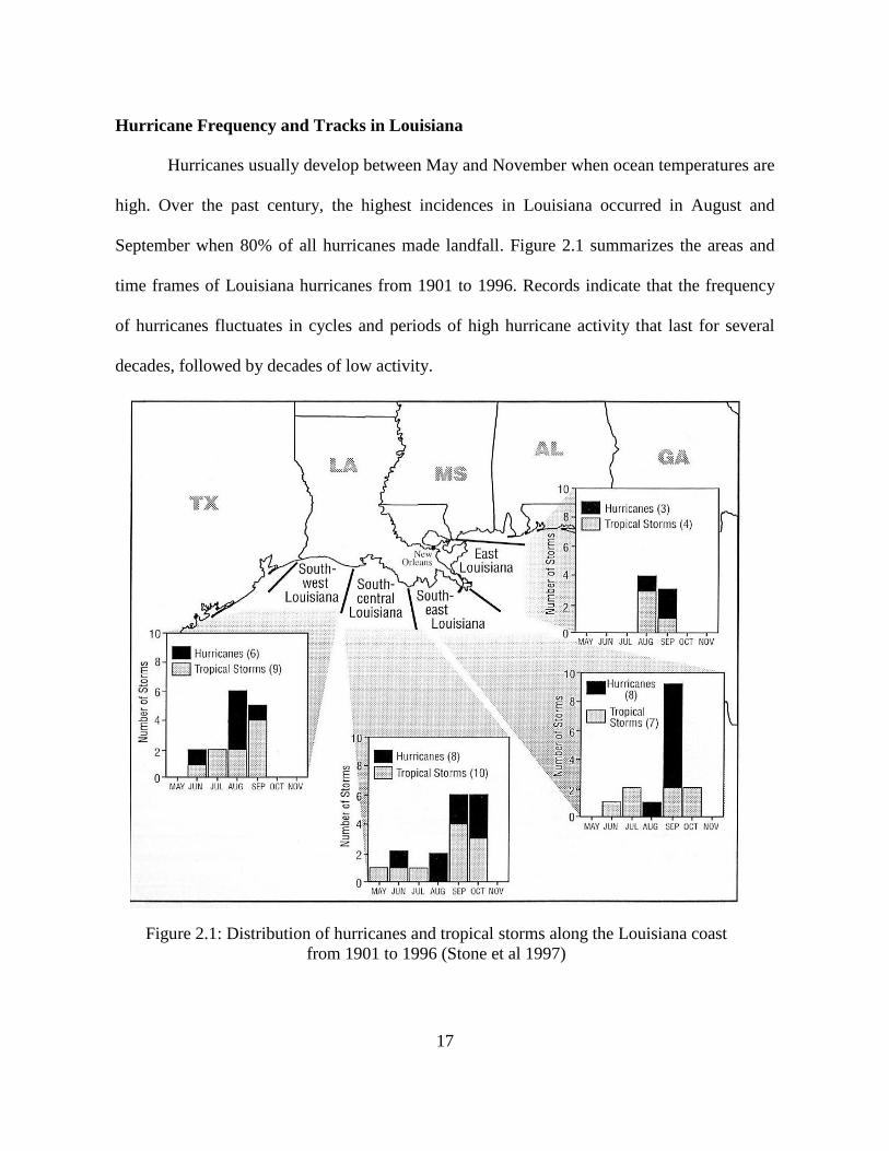
September when 80% of all hurricanes made landfall. Figure 2.1 summarizes the areas and
time frames of Louisiana hurricanes from 1901 to 1996. Records indicate that the frequency
of hurricanes fluctuates in cycles and periods of high hurricane activity that last for several
decades, followed by decades of low activity.
Figure 2.1: Distribution of hurricanes and tropical storms along the Louisiana coast
from 1901 to 1996 (Stone et al 1997)
18
The frequency of major hurricanes appears to rise and fall on a multidecadal time
frame. Approximately half of the number of tropical cyclones between 1901 and 1997 made
landfall within a 30-year period between 1931 and 1960. The decades before and after that
period experienced the landfall of only two hurricanes each (Stone et al. 1997). In the 1970s
and 1980s, tropical storm frequencies were low, and it was suggested that this might be
related to an intense and prolonged El Niño (Keim et al. 2004). Figure 2.2 shows the tracks of
the hurricanes, tropical storms, and tropical disturbances making landfall in Louisiana for the
years 1951 to 1996. The average number of hurricanes in the Gulf of Mexico between 1995
and 2005 has been unusually high. It appears that 1995 was the start of the latest natural
phase of high hurricane frequency, which is expected to persist for one or two more decades.
The hurricane season of 2005 exceeded all previously recorded activity for a single season.
2005 was the year with the most powerful hurricane ever recorded in the Atlantic basin
(Wilma) and the most destructive hurricane in U.S. history (Katrina). It also was the first time
that three category 5 hurricanes have ever been recorded in the same year in the Atlantic
basin.
Hurricane Impacts
The main impacts of hurricanes stem from wind, rain, and storm surge. The most
destructive impact of a hurricane is the storm surge which is the fast rise in the water level
that occurs when the hurricane approaches the coastline. The reasons for the increase in the
sea level are primarily low barometric pressure and strong winds that push the water towards
the coast. The storm surge is about one to six meters above sea level, and it is responsible for
about 90% of all hurricane related deaths and property damage (Allenstein 1985).

19
Figure 2.2: Tracks of hurricanes, tropical storms, and tropical disturbances to have made
landfall along or near the Louisiana coast from 1951-1996 (Stone et al. 1997)

20
Another component of a hurricane is the wind, which can cause significant damage. In
major hurricanes, flying debris is a hazard. The greatest impacts from winds occur to the east
of the eye at landfall since the wind speed on the east side of the storm is added to the forward
speed of the storm. Rainfall is another major hurricane effect and can cause heavy flooding of
inland areas which in turn leads to crop damage and destruction of highways, bridges, and
other structures. The impacts are often extensive if rivers flood their banks. Water runoff can
also be devastating in steep landscapes, where it leads to flash floods and mudslides. Finally,
hurricanes can create the conditions necessary for tornadoes. A tornado is a violently spinning
column of air shaped like a funnel that is in contact with the ground. Tornadoes are relatively
small with a diameter of around 100 m but their powerful winds are destructive and life
threatening.
Hurricane Forecast
Flood forecasting and warning systems have proven to be a valuable tool to mitigate
the adverse effects of a hurricane. Being able to predict hurricanes, disseminate warnings, and
evacuate appropriate areas can save lives, and even the economic losses have been shown to
be reduced by up to one third due to early warning (Smith 1996). Different hurricane and
flood forecast models have been developed. A hurricane model is usually a trajectory model
of the eye. The model considers the effects from the pressure gradient force, the centripetal
force, the Coriolis force, and surface friction. Based on these physical parameters, as well as
the topography and the bathymetry of the considered area, the prediction model calculates the
hurricane track, wind speeds, and the point of landfall. For real-time forecasts, meteorological
data has to be entered, such as latitude and longitude of the hurricane center, storm central
21
pressure, and radius of the maximum winds (Allenstein 1985). Hurricane models can be
coupled with storm surge models which include effects from the surface drag, eddy viscosity,
finite amplitude, and bottom slip (Jelesnianski et al. 1992). The National Hurricane Center in
Florida is the lead agency in the U.S. in hurricane prediction. The Center issues hurricane
watches and warnings if hurricanes become a threat to U.S. territory.
2.2 Louisiana's Wetlands
Louisiana's wetlands lie in flat coastal lowlands that are characterized by marshes,
swamps, lakes, levees, bays, and bayous. Not only does the coast present a unique landscape
with fabulous scenery and many opportunities for recreational activities revolving around
nature, fisheries, and wetland-based culture, but it also protects resources viable to the state
and the nation. With the deterioration of the wetlands, these resources are at risk.
Value of the Wetlands
What benefits do the wetlands provide? First, the marshes offer valuable hurricane
protection. Wetlands ameliorate the effects of the storms by slowing hurricanes down and by
reducing the storm surge. Second, the coastal areas are home to thousands of residents, who
live off the wetlands by farming, hunting, shrimping, crabbing, oystering, and fishing. These
residents have diverse national and cultural backgrounds. The Cajuns, the largest and oldest
immigrant group, were exiled Acadians from what is now Nova Scotia in Canada. Third, the
marshes are vital for the fisheries industry, particularly shrimp and oysters. Fisheries are
important for Louisiana, contributing over US$3 billion to its economy per year (COFCL
2002). Fourth, wetlands offer protection of oil and gas networks that are critical to U.S.
energy security. Fifth, other significant industries in the coastal area include petrochemical
22
processing and manufacturing, shipbuilding and repair, cargo, agriculture, and tourism
(Louisiana Coastal Wetlands Conservation and Restoration Task Force and the Wetlands
Conservation and Restoration Authority 1998). And finally, Louisiana's swamps represent a
unique ecosystem, providing habitat to many endangered species of flora and fauna.
Causes for Wetlands Deterioration
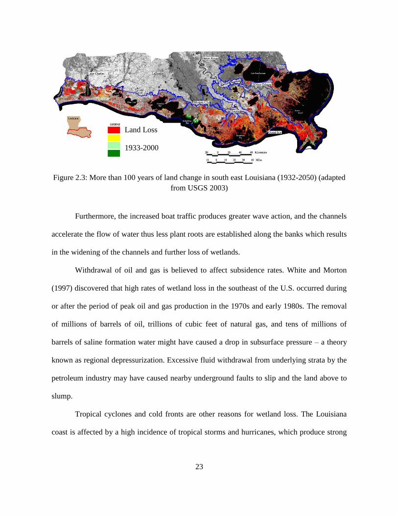
Natural and anthropogenic processes contribute to the land loss (Figure 2.3). One of
the main causes is the marsh's subsidence, i.e. the settling, decaying, and sinking of the soils
over time. The Mississippi River's spring floods once supplied Louisiana's coastland with
fresh layers of sediment which offset the subsidence and resulted in a balance of land loss and
gain. These annual floods, however, were often disastrous. The Great Mississippi Flood of
1927, for example, inundated an area of 70,000 km², caused millions of dollars in damages,
and killed several hundred people. Consequently, the levees were raised along the river and
lined with concrete, effectively preventing deluges and stopping the supply of the marsh-
building sediments onto the wetlands. Instead, the sediments are now channeled until they are
finally lost to the deep waters of the Gulf of Mexico.
The construction of canals through the marsh for oil and gas exploration and ship
traffic also contributes to the loss of wetlands. Since the 1950s, engineers have dredged more
than 13,000 km of canals, increasing erosion and allowing salt water to infiltrate brackish and
freshwater marshes. The salt infiltration destroys flora and fauna. The soils piled up on banks
act as barriers to the natural flow of water across the wetland, resulting in the flooding of
many areas.
23
Figure 2.3: More than 100 years of land change in south east Louisiana (1932-2050) (adapted
from USGS 2003)
Furthermore, the increased boat traffic produces greater wave action, and the channels
accelerate the flow of water thus less plant roots are established along the banks which results
in the widening of the channels and further loss of wetlands.
Withdrawal of oil and gas is believed to affect subsidence rates. White and Morton
(1997) discovered that high rates of wetland loss in the southeast of the U.S. occurred during
or after the period of peak oil and gas production in the 1970s and early 1980s. The removal
of millions of barrels of oil, trillions of cubic feet of natural gas, and tens of millions of
barrels of saline formation water might have caused a drop in subsurface pressure – a theory
known as regional depressurization. Excessive fluid withdrawal from underlying strata by the
petroleum industry may have caused nearby underground faults to slip and the land above to
slump.
Tropical cyclones and cold fronts are other reasons for wetland loss. The Louisiana
coast is affected by a high incidence of tropical storms and hurricanes, which produce strong
Land Loss
1933-2000
Predicted Land
Loss 2000-2003
Land Gain
1932-2000
Predicted Land
Gain 2000-2050
24
winds. The resulting elevated water levels and large waves lead to erosion, overwash, and
barrier breaching (Stone et al. 2004). For example, early estimates suggest that Hurricane
Katrina in August 2005 transformed approximately 80 km² of marshes into open water
(USGS 2005). Hurricanes can cause sudden and massive tree mortality and secondary damage
such as insect infestation and forest wildfires (Cablk et al. 1994). Moreover, Louisiana's high
frequency of cold fronts plays a critical role in generating and sustaining higher waves during
the winter months which again lead to shoreline erosion (Georgiou et al. 2005).
2.3 The Barrier Islands as Louisiana's First Line of Defense
Barriers are depositional elongated sand features for wave-dominated coasts that
extend above sea level (Roy et al. 1994). While they are usually shore-parallel bodies,
Louisiana's barriers no longer reside parallel to the shoreline but rather as offshore remnants
of former Mississippi delta lobes (Kulp et al. 2005). During tropical storms, these barrier
shorelines provide the first line of defense against large waves and storm surges by forming
protective structures for marshlands, estuaries, and the human infrastructure behind them. In
Louisiana, these features are threatened as they are rapidly degraded due to the above
explained reasons for wetlands deterioration. Another anthropogenic cause for the degradation
of the barriers is the construction of rigid concrete structures on the islands, which increase
erosion by increasing turbulences and velocity (Morton 2002).
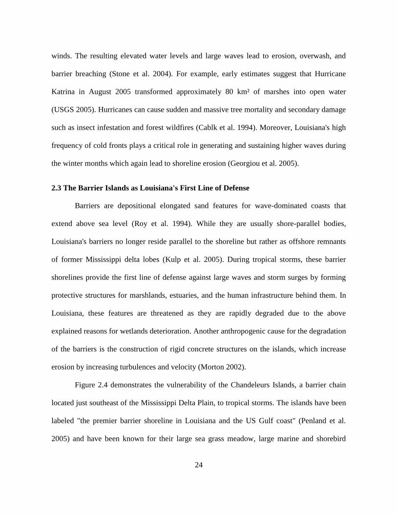
Figure 2.4 demonstrates the vulnerability of the Chandeleurs Islands, a barrier chain
located just southeast of the Mississippi Delta Plain, to tropical storms. The islands have been
labeled "the premier barrier shoreline in Louisiana and the US Gulf coast" (Penland et al.
2005) and have been known for their large sea grass meadow, large marine and shorebird
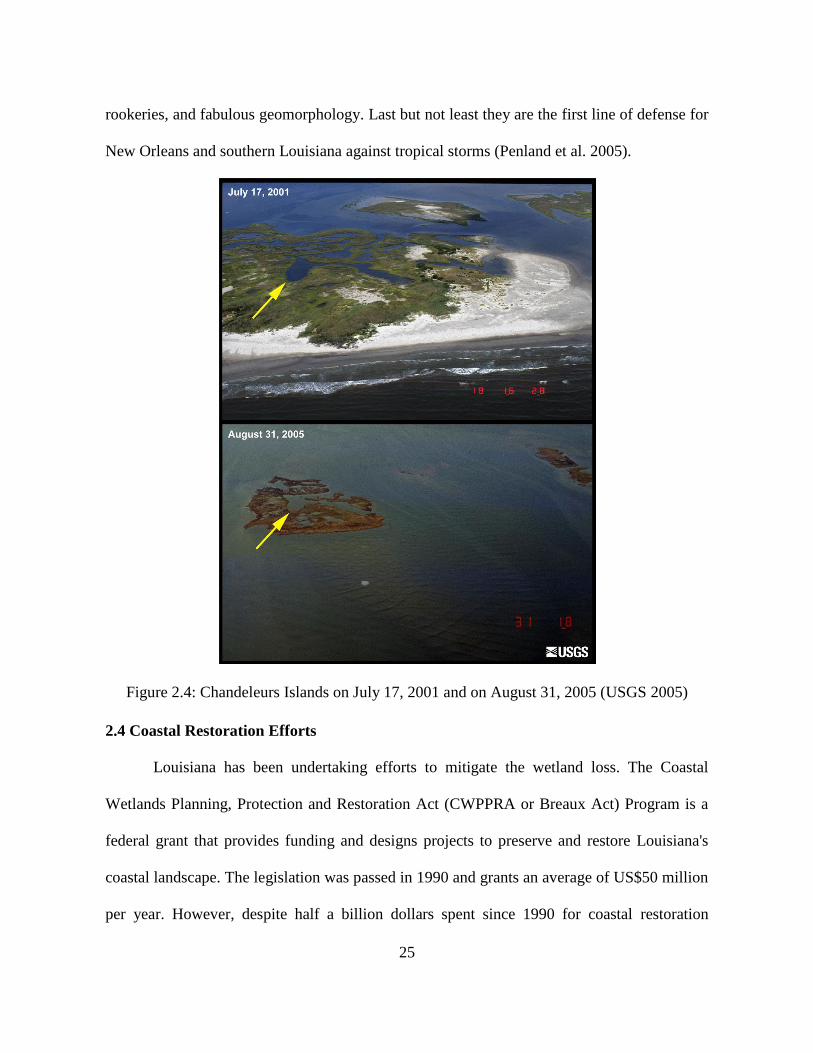
25
rookeries, and fabulous geomorphology. Last but not least they are the first line of defense for
New Orleans and southern Louisiana against tropical storms (Penland et al. 2005).
Figure 2.4: Chandeleurs Islands on July 17, 2001 and on August 31, 2005 (USGS 2005)
2.4 Coastal Restoration Efforts
Louisiana has been undertaking efforts to mitigate the wetland loss. The Coastal
Wetlands Planning, Protection and Restoration Act (CWPPRA or Breaux Act) Program is a
federal grant that provides funding and designs projects to preserve and restore Louisiana's
coastal landscape. The legislation was passed in 1990 and grants an average of US$50 million
per year. However, despite half a billion dollars spent since 1990 for coastal restoration
26
efforts, Louisiana continues to lose about 65 km² of land each year. To fully stop the land
loss, early studies suggest that US$14 billion over the next 20 years would be required
(Knapp and Dunne 2005). Is it feasible to raise such amounts of money? In November 2005,
roughly two months after Hurricane Katrina, the U.S. Senate passed a US$1.2 billion act to
fund coastal restoration and hurricane protection in the Gulf states. The money will be raised
from auctions of digital broadcast spectrum rights, with the auctions likely to take place in
2010.
Another hope for Louisiana stems from a pending budget bill that would channel a
share of federal offshore oil revenue to the coastal restoration efforts in the Gulf states. This
bill would provide Louisiana initially with several hundred million dollars a year, and it is
projected that the allocation would ultimately rise to US$2 to 3 billion per year (The Times-
Picayune 2005). Strategies to restore the marshes are not only costly but also politically
sensitive, since they affect communities, agriculture, and the petroleum industry. Numerous
mitigation strategies have been proposed. Most ideas include soft engineering solutions such
as coastal restoration through controlled flooding which involves cutting crevasses into the
levees that allow sediment diversions into the wetlands. Another approach entails distributing
dredged materials, which are obtained during channel maintenance, onto wetlands. Sediments
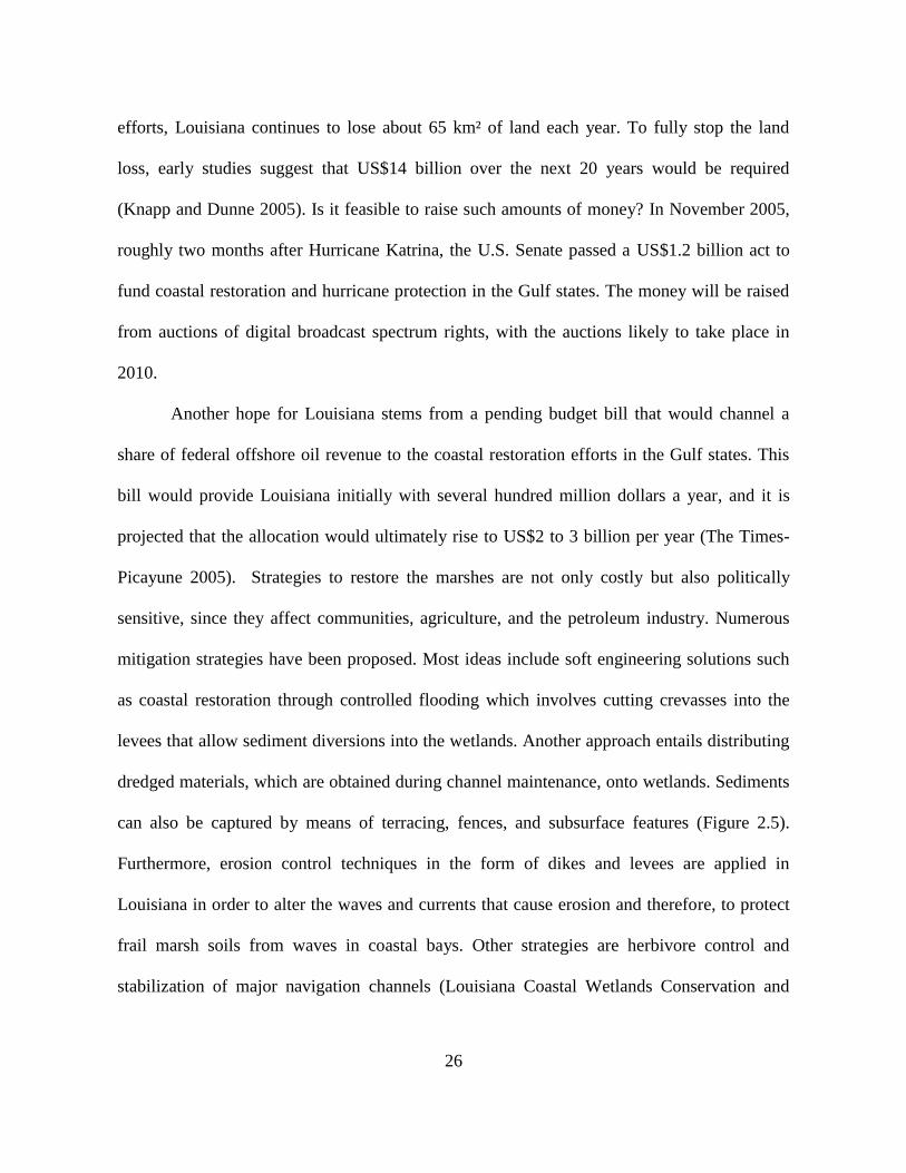
can also be captured by means of terracing, fences, and subsurface features (Figure 2.5).
Furthermore, erosion control techniques in the form of dikes and levees are applied in
Louisiana in order to alter the waves and currents that cause erosion and therefore, to protect
frail marsh soils from waves in coastal bays. Other strategies are herbivore control and
stabilization of major navigation channels (Louisiana Coastal Wetlands Conservation and
27
Restoration Task Force and the Wetlands Conservation and Restoration Authority 1998). In
order to stop the dramatic loss of the barrier islands, Campbell et al. (2005) propose seaward
beach berms, enhanced dunes, marsh platform restoration, and vegetative planting.
The costs and efforts to restore the wetlands are high but without the marshes,
Louisiana will lose many benefits, including storm defense, protection of the oil and fishery
industries, the conservation of unique cultures, and the preservation of a valuable ecosystem.
Figure 2.5: Terraces encourage sediment deposition and protect existing wetlands by reducing
wave action in the shallow waters of Little Vermillion Bay, Louisiana (NOAA 2004)
2.5 References
Allenstein, K. (1985). Land Use Applications of the SLOSH Model (Sea, Lake, and Overland
Surges from Hurricanes). Report No. 85-11. Chapel Hill, NC: Center for Urban and
Regional Studies (CURS), UNC.
Barras, J., S. Beville, D. Britsch, S. Hartley, S. Hawes, J. Johnston, P. Kemp, Q. Kinler, A.
Martucci, J. Porthouse, D. Reed, K. Roy, S. Sapkota & J. Suhayda (2003). Historical
and Projected Coastal Louisiana Land Changes: 1978-2050. USGS (United States
Geological Survey) Open File Report 03-334 (Revised January 2004).

28
Cablk, M. E., B. Kjerfve, W. K. Michener and J. R. Jensen (1994). Impacts of Hurricane
Hugo on a coastal forest: Assessment using Landsat TM data. Geocarto International,
2: 15-24.
Campbell, T., L. Benedet & C. W. Finkl (2005). Regional strategies for coastal restoration
along Louisiana barrier islands. Journal of Coastal Research, 44, 245-267.
Committee on the Future of Coastal Louisiana (COFCL) (2002). Saving Coastal Louisiana:
Recommendations for Implementing an Expanded Coastal Restoration Program.
Baton Rouge, LA: Governor's Office of Coastal Activities.
Elsner, J. B. & A. B. Kara (1999). Hurricanes of the North Atlantic: Climate and Society.
New York: Oxford University Press.
Georgiou, I. Y., D. M. Fitzgerald & G. W. Stone (2005). The impact of physical processes
along the Louisiana coast. Journal of Coastal Research, 44: 72-89.
Finkl, C. W. & S. M. Khalil (2005). Introduction. Journal of Coastal Research, 44: 2-6.
Jelesnianski, C. P., J. Chen & W. A. Shaffer (1992). SLOSH: Sea, Lake and Overland Surges
from Hurricane Phenomena. Technical Report NWS 48. Silver Spring, MD: National
Weather Service.
Keim, B. D., R. A. Muller & G. W. Stone (2004). Spatial and temporal variability of coastal
storms in the North Atlantic Basin. Marine Geology, 210: 7-15.
Knapp, B. & M. Dunne (2005). America's Wetlands: Louisiana's Vanishing Coast. Baton
Rouge, LA: Louisiana State University Press.
Kulp, M., S. Penland, S. J. Williams, C. Jenkins, J. Flocks & J. Kindinger (2005). Geological
framework, evolution, and sediment resources for restoration of the Louisiana coastal
zone. Journal of Coastal Research, 44, 56-71.
Louisiana Coastal Wetlands Conservation and Restoration Task Force and the Wetlands
Conservation and Restoration Authority (1998). Coast 2050: Toward a Sustainable
Coastal Louisiana. Baton Rouge, LA: Louisiana Department of Natural Resources.
Morton, R. A. (2002). Factors controlling storm impacts on coastal barriers and beaches - A
preliminary basis for real time forecasting. Journal of Coastal Research, 18: 486- 501.
Penland, S., P. F. Connor, A. Beall, S. Fearnley & S. J. Williams (2005). Changes in
Louisiana's shoreline: 1855-2002. Journal of Coastal Research, 44: 7-39.

29
Pielke, R. A. Jr. & R. A. Pielke Sr. (1998). Hurricanes: Their Nature and Impacts on
Society. New York: Wiley.
Roy, P. S., P. J. Cowell, M. A. Ferland & B. G. Thom (1994). Wave-dominated coasts. In
Coastal Evolution: Late Quarternary Shoreline Morphodynamics, eds. R.W.G. Carter
& C.D. Woodroffe, 121-186. Cambridge: Cambridge University Press.
Smith, K. (1996). Environmental Hazards: Assessing Risk and Reducing Disaster. 2nd
edition. London: Routledge.
Stone, G. W., M. J. Grymes III, J. R. Dingler & D. A. Pepper (1997). Overview and
significance of hurricanes on the Louisiana coast. Journal of Coastal Research, 13:
656-66.
Stone, G. W., B. Liu, D. A. Pepper & P. Wang (2004). The importance of extratropical and
tropical cyclones on the short-term evolution of barrier islands along the northern Gulf
of Mexico, USA. Marine Geology, 210, 63-78.
The Times-Picayune (2005). Senate OKs more money to save coast; but its bill differs from
House's in source of money. New Orleans, 4 November 2005.
United States Geological Survey (USGS) (2003). 100+ Years of Land Change for Coastal
Louisiana. [Retrieved from URL: http://www.nwrc.usgs.gov/special/landloss.htm].
United States Geological Survey (USGS) (2005). USGS reports new wetland loss from
Hurricane Katrina in southeastern Louisiana. Press Release, 14 September 2005.
White, W. A. & R. A. Morton (1997). Wetland losses related to fault movement and
hydrocarbon production, southeastern Texas coast. Journal of Coastal Research, 13:
1305-1320.
30
CHAPTER 3 : THE APPLICATION OF GEOTECHNOLOGIES AFTER HURRIC
THE APPLICATION OF GEO-TECHNOLOGIES AFTER HURRICANE KATRINA2
3.1 Introduction
While mainstreaming geo-information in disaster response is becoming increasingly
recognized as a key factor for successful emergency management, systematic knowledge
about the benefits and bottlenecks of geotechnologies in the response phase is still in fledging
stages. In the complex, dynamic, and time-sensitive disaster response situation of Hurricane
Katrina, geo-information enhanced decision-making and effectively supported the response
but it did not reach its full potential. The overwhelming complexity of the disaster exposed
challenges and highlighted good practices. Hurricane Katrina affected an area of nearly the
size of the United Kingdom (230,000 square km), it killed more than 1,700 people, and the
total cost of damage is estimated at more than $200 billion dollars. The destruction, which has
affected primarily the coastal regions of Louisiana, Mississippi, and Alabama, was caused by
high-speed winds, storm surge flooding in coastal areas, and, in New Orleans, also by levee
failures. Information management is a crucial component of emergency response. The ability
of emergency officials to access information in an accurate and timely manner maximizes the
success of the efforts. Since most of the information used in disaster management has a
geographic dimension (Bruzewicz 2003), geo-technologies have a large capacity to contribute
to emergency management. The capabilities of geo-technologies to capture, store, analyze,
2This chapter originally appeared as H. Brecht (2008), The Application of Geo-Technologies after Hurricane
Katrina, in Remote Sensing and GIS Technologies for Monitoring and Prediction of Disasters, eds. S. Nayak, S.
Zlatanova, Springer: 25-26. Reprinted with permission of Springer.

31
and visualize spatial data in emergency management have been documented in the literature
(Cutter 2003; Zlatanova 2006; Carrara and Guzzetti 1996). Paradoxically, in praxis the
convergence of the two fields of geo-information and emergency management is only
rudimentary developed and little work has been undertaken to enhance the integration.
What were the bottlenecks of using geo-information in the response phase of
Hurricane Katrina? Which mapping services were requested frequently? Which workflow
procedures streamlined the mapping support? What were the best practices? In the following
these questions are addressed focusing on five areas:
managerial lessons with regard to information flows and staffing issues;
the perfidies of technology infrastructures in an emergency situation;
important datasets and best practices of data documentation and access;
workflows that streamlined the mapping response;
the “stars” of the mapping products, which were requested or needed the most.
3.2 Lessons Learned
The knowledge about best practices was gained from the experience of GI responders.
Input was gathered mainly during the Louisiana Remote Sensing and GIS Workshop
(LARSGIS) in Baton Rouge, Louisiana, in April 2006 in which practitioners from the coastal
southeastern United States presented and discussed their experiences of using geo-
technologies after Hurricane Katrina. The author’s own experience in the Emergency
Operations Center (EOC) of Baton Rouge after the storm also influenced this paper.
32
3.2.1 Managerial Lessons
Improving Information Flows
Large amounts of data were acquired and processed after Hurricane Katrina. In the
immediate aftermath of the disaster, governmental agencies and private geo-technology
companies, realizing the extent of the damage and the gravity of the situation, supported the
relief efforts by contributing data. Numerous sets of aerial photographs were taken and
distributed to assess flooding and damage, private companies donated satellite images, data,
and hardware, and new data layers concerning emergency shelters or power outages were
created. Public agencies released and shared existing but previously undisclosed data layers.
The usual obstructive administrative barriers caused by competition and conflicts between
divisions were abrogated, and instead ad-hoc alliances were built to support the common goal
of saving lives and containing the devastation. Data streamed in quickly, resulting in the
availability of a multitude of new data layers. The dissemination of the data to the appropriate
parties at the desired locations in a timely manner, and in a useful format may have been the
biggest challenge for the GI response community. Agencies were not always aware which
information was available or where to find certain data. Due to miscommunication, excessive
workloads, and general distress, information was distributed only to a limited extent and did
not always reach the first responder crews or county governments in remote areas that were in
crucial need of this information.
Information flows and structures between the different actors must be identified before
the disaster. One possible strategy is to appoint a central data authority that collects and
disseminates information, a solution that is effective but difficult to realize due to political and
33
economic reasons. Spatial data infrastructures and web-based solutions have proven to
enhance information flows and data accessibility. These tools should to be established before
the disaster strikes.
Establishing Geo-Technologies as an Integral Resource
Mapping support often evolved as an ad-hoc component after the storm being
triggered by a high demand for maps and geo-information. Impromptu volunteers were
engaged or geo-information companies were hired on the spot. Emergency preparedness units
need to recognize geotechnology as crucial part of disaster management and incorporate it
accordingly into their planning. It is the task of the GI community to increase the awareness
of emergency managers towards the value of spatial technology. During the emergency,
knowledge gaps became apparent on both sides: governmental emergency staff was unclear
about the potential of geo-technologies and the use of maps and the GI community was not
informed about governmental disaster plans and strategies. Both parties have to gain an
increased understanding of each other’s duties and capabilities. Communication and training
platforms are means to enhance awareness.
Building Partnerships
Formal and informal partnerships between GI professionals that were established
before the disaster proved to be essential in the disaster response. Relationships facilitate
coordination and thus the flow of information. One way to strengthen collaboration is the
establishment of a workgroup of GI-skilled personnel in governmental agencies, universities,
and private industries. Regular meetings foster networks and enable the exchange of news
about available data and technologies.
34
Identifying Staff
GI responders were confronted with many requests for maps and an understaffing in
the EOCs. It proved valuable to call on the support of GI colleagues. Volunteers played an
important role in the response to Katrina, and it is recommended to integrate them into
emergency planning. Staff to support operations during an emergency needs to be identified
beforehand. If a disaster occurs, a call-up of pre-defined GI- skilled personnel should be
initiated to set up teams. The response teams should include staff from different governmental
departments and from academia, assembling specialists from the different fields in geo-
technology, such as remote sensing, programming, databases, and GIS. It is helpful to assign
staff certain responsibilities pertaining to data collection, logistics, technical support,
mapping, distribution, and operational management. Specific staffing challenges are caused
by the 24 hours per day, seven days per week operations which require a high staff rotation.
For the rotation not to affect efficiency, detailed documentation of requests, actions, files, and
file locations are necessary.
3.2.2 Technology Infrastructure Lessons
Ensuring Hardware Resources
The EOCs were not or only rudimentary equipped for geo-technologies prior to
Hurricane Katrina. Computers, plotters, printers, and other supplies had to be identified and
installed after the storm. Difficulties occurred with regard to finding space in the EOCs not
only for large hardware devices and storage systems for hard-copy maps, but also for laptops
and workstations. Mapping teams should establish sources and localities of all necessary
hardware beforehand and explain their special demands so that physical space in the EOCs
35
can be allocated. In the response to Hurricane Katrina, innovative solutions were found, such
as the one from a mapping team in Mississippi that remodeled a bus into office space and
equipped it with workstations and printers.
Securing Continuity of Operations
Useful datasets were stored on computers that flooded or that were left behind in the
evacuation. Data back-ups at multiple secure locations and mobility of hard- and software are
to be established to enable continuous operations under emergency conditions and to avoid
loss of data. Data accessibility was not only hampered by disrupted networks and flooded
computers but also by logistical issues. In one case, important files were password protected
and the responsible administrator could not be reached.
Preparing for Power and Network Disruptions
Power, network, and internet outages were frequently encountered. Ideally, alternative
power supply solutions are identified beforehand, including generators and uninterruptible
power supplies (UPS) with battery backups that can be added to hardware devices to avoid
data losses during power disruptions. Since it is not advisable to rely on network connectivity,
sufficient data sharing devices are necessary for an efficient response. Moreover, regular
back-up mechanisms proved to be valuable.
Administering Networks
Not only GI skills were vital for successful operations but GI staff installed
intermittent network routers, virtual private networks and other network connections. Ideally,
a network administrator is appointed who is in charge of connectivity issues.
36
3.2.3 Data Lessons
Acquiring Relevant Data
Base datasets, for example on pumping stations, utility networks, and power plants,
were not always readily available. Especially for rural areas, geo-information was scarce.
Information that proved to be of focal interest during the emergency can be divided into two
categories: information that should to be collected before the disaster and information that is
to be collected after the disaster.
Datasets that were vital during the response and that can be acquired before the
disaster include but are not limited to:
Pumping stations Hazardous materials
Street maps Building footprints
Elevation models Helicopter landing places
Points of interest Special needs population
Fire stations Evacuation routes
Cadastral data Population densities
Medical centers Day and night population
Geomorphology Utility networks
Land use Emergency resources
Power plants Address dataset
Satellite imagery
Datasets that were frequently requested in the EOCs providing information on the extent of
the catastrophe include but are not limited to:

37
Wind fields Oil spills
Power outages Flood depths
Debris estimates Levee breaks
Daily dewatering Road restoration
Power restoration Emergency shelters
Flood fatalities Flood extent
Satellite imagery Fire outbreaks
Deceased victim locations Points of dispensing
Restored power Pollution
Crime scenes Damage estimates
Sources need to be established for information that becomes available after the
disaster. This can be accomplished with data sharing agreements, which should be set up prior
to the emergency. These agreements determine which data will be provided by which
organizations and who holds copyrights. For instance, uniform, useful, and complete image
datasets were in high demand after Katrina. Therefore, contracts with companies providing
aerial photography should be in place, specifying resolutions, area coverage, formats, geo-
correction procedures, and accompanying metadata. Agreements need to include how often
datasets will be updated since some of the mentioned data layers require daily updates. For
instance, shelter locations opened rapidly in the immediate aftermath and then, after a few
weeks, closed or moved. Information on flooded roads also needed daily updating, as did the
locations of crime scenes.

38
Clarifying Copyrights
The clarification of data copyrights and privacy laws was time consuming. It was
difficult to reach those in charge to get permission for data dissemination because
communication networks were interrupted, electronic address books were inaccessible due to
flooded and left behind computers, and officials were dispersed because of the evacuation or
not available during the weekend and at night. It is of advantage to negotiate data
dissemination agreements, data sharing policies, and specifications of data custodianship
before the disaster.
Collecting Metadata
After Hurricane Katrina, a multitude of datasets were disclosed and created rapidly.
Maps showing the newly available information were requested, produced, and distributed in
extremely short time spans. A central problem that arose from this incoming data stream and
the stressful situation was that metadata tended to be neglected. However, crucial information
is rendered unemployable if datasets are not properly documented.
Moreover, metadata helps to maintain standards for data quality. Finally, missing
metadata causes delays since valuable time is spent struggling to find out, for example, on
which date an aerial photo set was taken and which area it covers. A metadata standard should
be chosen that answers questions of data timeliness, source, accuracy, and coverage. Although
metadata collection is time-consuming, GIS staff receiving data must be dedicated to
metadata collection, ensuring that a predefined form is completed for all incoming datasets. A
data manager should be assigned whose responsibilities include documenting metadata.

39
Organizing Data
In the response phase, geographic information must flow upstream and downstream
between players in real-time. An effective means of accomplishing this dissemination of data
is a spatial data infrastructure (SDI) which enables an efficient, reliable, and secure way for
the search, exchange, and processing of relevant information. An SDI is a framework that
subsumes a collection of geospatial data, technologies, networks, policies, institutional
agreements, standards, and delivery mechanisms. Creating an infrastructure subsuming both
general and emergency-related data with clearly laid out directory structures and logical
names is critical for effective emergency response where many applications occur in real-
time. The SDI datasets need to be updated continuously, and data integrity has to be
maintained. The responsibility of data creation and maintenance for the SDI cannot lie with
one individual organization; it must rather be a joint effort of many organizations.
3.2.4 Operational Lessons and Workflows
Avoiding Duplication of Efforts
Duplication occurred when maps, conveying identical information (e.g. damage levels,
road flooding, or power outages), were created by several agencies. Coordination via the
implementation of a map depository where central players submit and download maps is a
possible solution to this duplication.
Tracking Requests
Keeping track of map requests was conventionally handled by means of paper files. In
the Baton Rouge EOC, a team from the Louisiana State University implemented an online
tracking system that largely improved the paper system. This tracking system not only

40
documented the actual request but also associated information including contact information
of the client, file locations, and map products. The system allowed efficient communication
with all members of the response team, which was particularly important due to the high staff
turn-over and geographically distributed mapping operations. The documentation of file
locations and templates was especially helpful for the preparation of the daily updates of
certain maps such as road flooding and emergency shelters. Another feature of the system
allowed personnel to be assigned to the various projects. Such a record system for requests,
associated files, documents, staff, clients, and products proved to be useful and should be
implemented before the disaster strikes.
Preparing Paper Maps
Despite increasing digitalization, paper maps were still essential for the response
teams. A high demand of paper maps and only limited printing and plotting capacities caused
delays in fulfilling requests and disseminating information. Base maps, especially street maps
on different scales, can be prepared beforehand. Ensuring access to sufficient amounts of
paper, printers, and plotters is crucial.
Creating Templates
Map templates were found to be useful in the response activities. In the case of daily
updated information, consistent templates accelerated the creation of maps and facilitated the
comparisons of changes. Predefined map templates containing many data layers, which are
turned on and off according to specific needs, saved a considerable amount of time. The
templates should be well documented and logically stored within the data structure.
41
Disseminating GIS Resources
While staff on site in the EOC took requests, promoted geo-technologies, offered
solutions, and generated quick maps, staff in remote locations was able to create more
sophisticated maps and provide analysis away from the bustle in the EOC. This approach also
guaranteed access to hardware, especially printers, that were not backlogged as was often the
case in the EOCs.
Using Online Tools
Web-based tools such as Mapquest or Google Earth, were used intensively in the
response operations. Not only the GI staff but many of the involved responding agencies and
rescue workers applied especially Google Earth for their operations. Google Earth and Google
Maps created satellite imagery overlays of the devastation in the affected region, which
helped to understand the scope of the disaster. Single houses and addresses could be looked
up in Google Earth, and a built-in transparency slider, which allowed to switch between
before and after images, enabled to see if and how much damage a place experienced. The
accuracy and the ease of use of these online tools that can be operated by non-GIS staff
contributed to the wide usage of the tool. This experience highlighted the potential of a web-
based community approach to disaster operations.
Promoting Geo-Information
Since rescue workers were often not versed in the potential of geoinformation, it was
useful to have a GI staff member attend official EOC meetings to offer GI-based suggestions
and solutions. Another way to convey the GI services to officials was by means of fixing
frequently requested maps on the walls or collecting them in a map book for display.
42
3.2.5 Map Products
Requests from Emergency Responders
The large majority of requests from emergency responders were related to street
atlases and area overview maps. Commercial maps in stores sold out quickly or flooded and
therefore, responders relied on the GI community. Great numbers of street maps were handed
out after the storm. The acquisition of digital copies of city maps from commercial companies
was helpful. Emergency responders who were not familiar with the area requested maps with
photos of landmarks such as the New Orleans Superdome. Checkpoints, which were still
standing after the storm, were included in the produced maps. This concept proved to be
remarkably helpful for an orientation of the area especially since many street signs were
flooded or destroyed. Another crucial orientation and communication means is a grid system
for ground reference. After the disaster, some responders considered missing grids in maps as
one of the central problems. It would be helpful if map books in compact sizes with the
standardized US National Grid, street indices, landmarks, and elevation levels are produced
before the disaster. Overlaying street and area maps with satellite inundation maps that outline
the extent of the flood and the flood depth was another frequent request. For instance, by
means of this data, rescue missions determined whether boats or high-water vehicles are used
in a certain area (Figure 3.1).
For the search and rescue operations, mapping of addresses and coordinates of victims
was of major importance in the first days after the disaster. Ideally, this process would be
automated. Coordinates from a mobile phone placing a 911 call could be tracked

43
automatically and then transferred to handheld computers of emergency responders. Geo-
technology can calculate the best routes for accessing victims’ locations.
Figure 3.1: Illustration of the depth and extent of the inundation on August 31, 2005, caused
by Hurricane Katrina (NOAA 2005)
The Needs of the Public
Accurate and timely information for the public is necessary. The questions of if a
house was damaged plagued the evacuees. Days after the disaster, in order to find out if and
how deep a house was flooded, the evacuated population relied on photos from television and
the Internet to recognize neighborhoods and the levels of flooding and destruction. The
uncertainty added to stress and anxiety. This information could be conveyed using web
mapping and aerial photographs taken after the disaster.
Vector layers with flood depths and levels of wind damage can complement the
information. A system could be established that allows people to enter the address of a
building to find out water depths, damage levels, when and how they could travel to the
44
building, and nearest emergency supply centers. Moreover, the public requires detailed
knowledge about the assigned evacuation routes and the traffic circumstances, evacuation
shelters, kitchens, health facilities, and other public services.
Requests from Government Officials
Government officials asked for maps with various contents, including shelter
locations, deceased victim locations, power outages, water systems, maps of state-owned
land, pumping locations, and others.
3.3 Conclusions
This paper identifies lessons learned from the application of geotechnologies in the
response to Hurricane Katrina. The main challenges in the operations were not related to the
often discussed literature themes such as interoperability and semantics but rather to trivial
issues such backlogged printers, network disruptions, and missing metadata. Aloof from
Virtual Reality applications, one of the most frequent tasks of GI personnel was to print street
books and visualize search and rescue coordinates.
Truly analytical GI applications going beyond simple map displays were sparse.
Experience shows that the suitability and use of GI technology in the response phase differs
from the planning phase because of the urgency, uncertainty, the magnitude of stakeholders,
some of whom are unfamiliar with geo-information, and the real-time data needs. Among the
most useful GI products created were inundation maps and map books with landmarks,
detailed elevation figures, and unified grid systems.
Web-tools such as Google Earth proved to be helpful due to their relevancy, ease of
use, and open access. There are reasons to believe that the field of geo-information for
45
disaster management will eventually benefit from further developments of visual
environments, semantic interpretations, and other current research topics. Most likely, the
future use of geotechnologies will extend beyond mapping and move towards analytical
processes. This will especially be the case when emergency managers gain knowledge in geo-
information and its capabilities. Currently, however, improvements on the ground are
necessary on basic levels. Other analyses of geo-information in disaster management (Kevany
2003; Zerger and Smith 2003; Curtis et al. 2005) report similar experiences, stressing the
practical impediments of implementations. Existing knowledge about best practices need to
be translated into action, programs, and relevant policies. To enhance the response, the often
separate discourses of geo-technology on the one hand and emergency management on the
other need to converge.
3.4 References
Bruzewicz, A. J. (2003). Remote sensing imagery for emergency management. In
Geographical Dimensions of Terrorism, eds. S.L. Cutter, D.B. Richardson & T.J.
Wilbanks, 87–97. London: Routledge.
Carrara A. & F. Guzzetti (eds.) (1996). Geographical Information Systems in Assessing
Natural Hazards. Dordrecht, The Netherlands: Kluwer.
Curtis A., J. W. Mills, J. K. Blackburn & J. C. Pine (2006). Hurricane Katrina: GIS Response
for a Major Metropolitan Area. Quick Response Report QR180. Boulder, CO:
Natural Hazards Center, University of Colorado.
Cutter, S. L. (2003). GI Science, Disasters, and Emergency Management. Transactions in
GIS, 7: 439-445.
Kevany, M. J. (2003). GIS in the World Trade Center attack – trial by fire. Computers,
Environment and Urban Systems, 27: 571-583.
Zerger A. & D. I. Smith (2003). Impediments to using GIS for real-time disaster decision
support. Computers Environment and Urban Systems, 27: 123-141.

46
Zlatanova S., P. Van Oosterom & E. Verbree (2006). Geo-information Support in
Management of Urban Disasters. Open House International, 31: 62-69.
47
CHAPTER 4 : A GLOBAL URBAN RISK INDEX
A GLOBAL URBAN RISK INDEX
4.1 Introduction
The potential for losses from natural hazards is particularly high in urban areas. 1.5%
of the world’s land is estimated to produce 50% of worldwide Gross Domestic Product
(GDP). The same area accommodates about one sixth of the world’s population (World Bank
2009). Concentrations of population, industry, infrastructure, and economic activities in cities
contribute to increased exposure and susceptibility to natural hazards. In fact, the ongoing
process of urbanization is one of the main reasons for the staggering increase in disaster death
tolls and economic losses over the past decades (e.g., Quarantelli 1996, Wisner 2003, Pelling
2003).
The impacts from disasters are on the rise. Statistics show that, even when adjusted for
inflation, the losses caused by natural catastrophes have been increasing dramatically and at
an ever-quickening pace since 1950. In the period between 1990 and 1999 the costs of
disasters in constant dollars were more than 15 times higher than during the period 1950-59
(World Bank 2006). The number of people affected by natural hazards each year nearly
quadrupled from 1975-84 to 1996-2005 (EM-DAT 2007). Several factors contribute to this
increase, for example land use changes, social inequalities, subsidence, and environmental
degradation (e.g., Smith 1996, Mileti 1999, Blaikie et al. 1994). Some scientific studies
suggest that a rise in hazardous events can be attributed to climate change (e.g., Emanuel
2005, Bengtsson et al. 2006, Vermeer & Rahmsdorf 2009). But the main driver of risk is
population pressure, which is spreading in vulnerable locations, for example, in coastal areas
48
susceptible to cyclones. The world’s low lying coastal elevation zone covers 2% of the
world’s land area but contains 10% of the world’s population (McGranahan et al. 2007). Due
to the global urbanization process, cities are becoming increasingly predestined for risks.
Estimates by the United Nations suggest that over 50% of the world’s population already lives
in urban areas (UN 2008). Cities are predicted to absorb most of the future growth in the
world population: the UN estimates that the urban population share will rise to 70% by 2050
(UN Population Division 2007).
While natural hazards and ongoing urbanization are inevitable, disaster losses can be
minimized through adequate disaster risk management. Reducing risks ex-ante through risk
assessments, land use planning, building codes, early warning systems, adequate watershed
management, and contingency planning leads to significantly reduced disaster impacts. The
earthquake in Chile in March 2010 was one of the ten most powerful earthquakes recorded in
the last century. It released 500 times more energy than the earthquake that struck Haiti in
January 2010. Yet, only 521 people died in Chile, whereas Port-au-Prince was
catastrophically affected with tens of thousands of deaths. The main reason for this difference
is that buildings in Chile are built to codes and are regularly inspected whereas Haiti
effectively has no building codes.
Because of the enormous loss potential that has developed and is expanding in the
narrowest of urban space, disaster risk reduction efforts need to be intensified in cities.
Especially developing countries are suffering from the consequences of disasters with more
than 95% of disaster deaths occurring in the developing world in the past quarter century
(Arnold & Kreimer 2004) and with economic losses being 20 times greater as a percentage of
49
GDP in developing countries than in developed ones (World Bank 2006). To secure the
steady advances towards poverty alleviation and economic growth in the developing world,
suitable risk reduction strategies must be developed and mainstreamed into urban planning
and development strategies. Otherwise, years of development and accumulated wealth are
repeatedly destroyed and eroded through repeated disasters.
Given the intrinsic high loss potential from natural hazards in urban areas, it comes as
a surprise that little is known about the vulnerability and risk potential of cities. Which cities
are likely to be affected by a disaster? In which cities is the risk of mortality due to disasters
the highest? Which cities are most at risk of economic losses due to natural hazards? Efforts
to assess urban risks so far have mainly focused on single cities, identifying inner-city
hotspots. But a comprehensive ranking of the global cities’ risk to guide priorities in building
resilience has been lacking. This study creates, for the first time, a disaster risk ranking of the
main cities in the less developed world. Risk levels of 1,943 cities in 110 countries are
evaluated and compared. The five following features characterize the index:
Risks are assessed for urban agglomerations with more than 100,000 inhabitants.
For each city, mortality risk and economic risk are calculated by taking into account
three components of risks: hazard, exposure, and vulnerability.
The loss potentials are expressed in relative levels.
Four major natural hazards, namely earthquakes, cyclones, floods, and slides are
considered in this study. Urban risks are identified for each of these hazards
separately. In addition, a multi-hazard index gives a holistic picture of city risk.

50
Expected urban risk exposure in the year 2050 is determined through projections of
future city population growth.
By disclosing risks to cities, we hope to raise awareness, inform resource planning,
inspire further research, particularly at local levels, and promote the shift towards managing
risks rather than emergencies.
4.2 Background
The assessment of risk is highlighted as a central activity in defining priorities and
building resilience in the Hyogo Framework for Action 2005-2015 (UN-ISDR 2005), signed
by 168 nations and international organizations at the 2005 World Conference on Disaster
Reduction. Risk identification supports a wide range of decision-making processes for
different actors on how risk should be managed from the public to the private sector (e.g.,
Cutter & Finch 2008, Birkmann 2006, Fuessel 2007). Quantifying risk and estimating future
losses are not only the first steps in any disaster risk reduction program; the resulting
scenarios of a risk assessment are increasingly incorporated into sustainable development
approaches in different sectors in order to climate- and disaster-proof investments. Once the
severity and geographical extent of risks have been assessed and the drivers of risk are better
understood, appropriate and cost-effective countermeasures can be systematically identified
and implemented. Depending on the scale, risk assessments support multiple applications, for
example, urban planning, investment prioritization, land use planning, building codes, and
disaster risk financing solutions.
A range of perspectives on risk assessments and indices has emerged, ranging from
quantitative calculations on losses to qualitative analysis capturing also intangible impacts.

51
Interesting initiatives have developed mainly on national level but a few have also been
completed on global and urban scale.
Global level: Two main risk assessments initiatives have been undertaken with the
goal of identifying multi-hazard risk worldwide on the basis of grid cells with sub-national
extent. First, the Global Disaster Hotspots, developed by the World Bank and Columbia
University (Dilley et al. 2005, Lerner-Lam 2007) produced detailed geospatial data on risks of
mortality and economic losses for six major natural hazards. The results enabled a global
assessment of risk levels and the identification of areas where the potential for disaster
impacts is large. Second, the Global Assessment Report 2009 (UN-ISDR 2009) is a multiple
agencies effort that developed the Global Disaster Hotspots further by using enhanced
modeling techniques and improved data layers. An update of this 2009 global risk analysis
was released in the Global Assessment Report 2011 (UN-ISDR 2011).
National level: An example of a comprehensive multi-hazard risk index that assigns
overall risk values on a national level is the Disaster Risk Index (DRI) (Peduzzi et al. 2009).
The DRI calculates three factors on a national resolution for 200 countries: risk of mortality,
the relative vulnerability of each hazard type, and the physical exposures of populations to
hazard. Another example for a risk assessment on national scale, covering a multitude of
countries, is the study by McGranahan et al. (2007), which ranks countries according to their
population shares in the low elevation coastal zones.
Urban level: With the rise of megacities, risk assessments have increasingly taken
place on city-level, identifying inner-city areas of high risks and loss potential (e.g., World
Bank 2010). However, only a few limited initiatives exist which assess the overall risk of
52
numerous cities in the form of an index to compare and rank cities with each other. Efforts in
this area to date have been confined to relatively limited sets of locations and hazards. The
Munich Reinsurance Group developed the Natural Hazard Index for Megacities for 50 cities
with high global economic significance (Munich Re 2005). The index has an economic
emphasis and is geared towards the risk of material losses which is suitable from an insurance
perspective. Hanson et al. (2011) ranked 136 port cities around the world that have more than
one million inhabitants. The study examines the risks of coastal areas due to storm surge and
high winds, taking into account predictions of climate change, subsidence, and population
growth. Brecht et al. (2012) determined the impact of sea level rise and intensified storm
surges in developing countries and highlight the major cities worldwide that are located in
storm-surge zones. Furthermore, methodologies have been developed that propose indicators
to estimate the overall risk of cities. Indicators, include, for example, population density or
number of hospital beds (e.g., Davidson 1997, Cardona 2005). These methodologies are
frameworks that were selected without regard to data availability and they have been
implemented only for a handful of cities.
4.3 Motivation
Why is a global urban risk index important? There are a number of ingredient
questions here. One question is whether an index is useful. Indices consist of a set of
indicators, which are derived from extensive datasets that are mathematically combined. An
index aggregates information and summarizes a body of knowledge from a wide range of
disciplines. It filters information for the reader and translates research into easy to understand
results. This makes indices appealing tools, which are widely used.
53
An additional question is whether a global risk index is of value. A risk index
combines complex data of hazards, vulnerabilities, and exposure. One advantage of such an
index is that it enables the comparison of risk levels in a self-explanatory manner. As the
international development community gradually shifts from financing post-disaster relief
towards financing disaster prevention (see for example, Ashdown 2011), a global risk index
gives reference points for investment decisions. It enables a comparison of risk levels
worldwide and yields the basis for decisions on where funding for disaster risk reduction
should be allocated. It allows comparability and the prioritization of programs in areas where
hazard risk is greatest and where investment benefits are maximized. Cutter (2001) stresses
that geographic comparisons across regions with a systematic approach in methodologies and
data are crucial to prioritize risk reduction strategies or poverty reduction goals. Yet, disaster
research has usually gravitated toward group or community studies as opposed to large-scale
projects (Tierney 2002). Second, by disclosing risks, we intend to raise awareness with regard
to potential disaster losses and promote the shift towards managing risks rather than
emergencies. A global risk index is helpful for showing planners at which level they are. It
gives an understanding of risk and has the innate potential to sensitize the public and
encourage officials to take action. And third, we hope that the index will stimulate more
detailed research on where the risks are, what the main drivers of risk are, and where to invest
to minimize vulnerability.
Finally, another question relates to the advantages of an index that concentrates on
urban areas. Urban areas are the fastest growing areas on earth. The world’s population
became predominantly urban in 2009 with over 50% living in cities, and the UN estimates
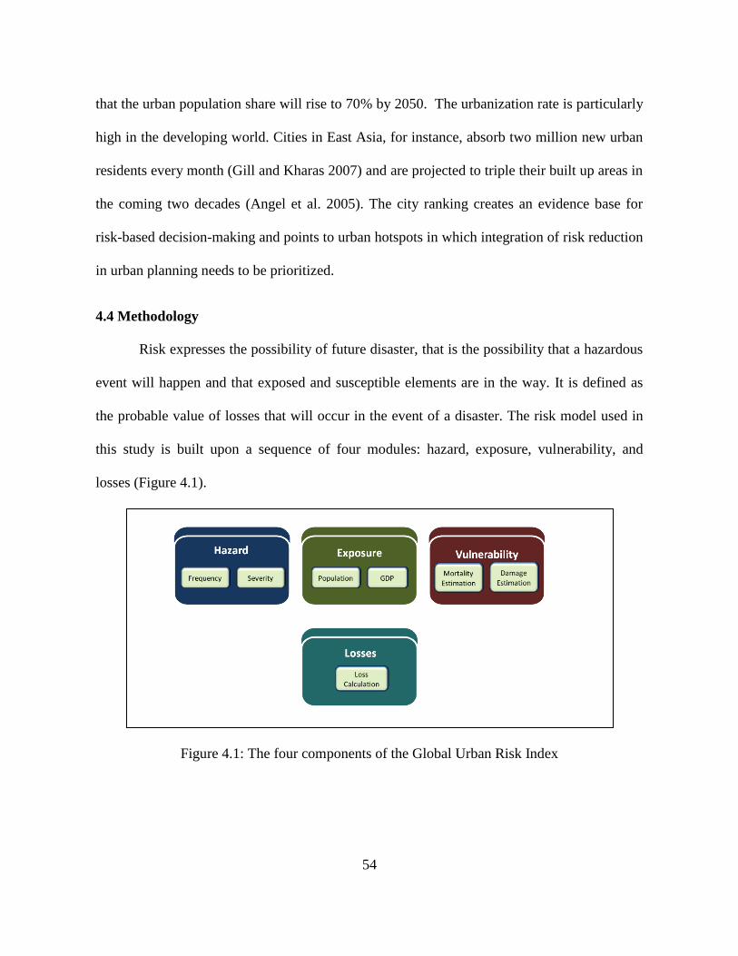
54
that the urban population share will rise to 70% by 2050. The urbanization rate is particularly
high in the developing world. Cities in East Asia, for instance, absorb two million new urban
residents every month (Gill and Kharas 2007) and are projected to triple their built up areas in
the coming two decades (Angel et al. 2005). The city ranking creates an evidence base for
risk-based decision-making and points to urban hotspots in which integration of risk reduction
in urban planning needs to be prioritized.
4.4 Methodology
Risk expresses the possibility of future disaster, that is the possibility that a hazardous
event will happen and that exposed and susceptible elements are in the way. It is defined as
the probable value of losses that will occur in the event of a disaster. The risk model used in
this study is built upon a sequence of four modules: hazard, exposure, vulnerability, and
losses (Figure 4.1).
Figure 4.1: The four components of the Global Urban Risk Index

55
4.4.1 Assessing Hazards
Hazard refers to the possible occurrence of physical events that may have adverse
effects on vulnerable and exposed elements (White 1973). The hazard module in this index
assesses the risks from four different natural hazards: earthquakes, landslides, floods, and
cyclones. Risks are determined for each hazard individually and a multi-hazard index gives an
overall picture of city risk. To estimate the likelihood of a hazard striking a given city, this
study has taken advantage of global hazard data sets developed by different organizations
(Table 4.1).
The data sets depict the geographic distribution of hazard risk in a grid format with
resolutions of 1 km2. Hazard frequency and, when available, severity were derived from
historic events, from modeled probabilities or from a combination of both. Historic events
have been used to calculate cyclone hazard risk for cities. To estimate cyclone risk, more than
2,800 historic cyclone tracks in the time period from 1975 to 2007 and their modeled wind
speed plumes were calculated (Figure 4.2) and combined, resulting in a global grid, that
shows how many times each grid cell has been struck by a cyclone (frequency) and with what
wind speed (severity) (Figure 4.3).
To calculate landslide hazards, probabilities were applied. The probabilities were
derived through a combination of trigger and susceptibility factors defined by various
parameters, including slope factor, lithological or geological conditions, soil moisture
condition, vegetation cover, precipitation, seismic conditions, and Shuttle Radar Topography
Mission (SRTM) elevation data.
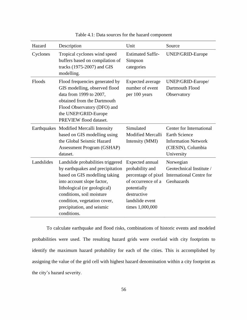
56
Table 4.1: Data sources for the hazard component
Hazard Description Unit Source
Cyclones Tropical cyclones wind speed
buffers based on compilation of
tracks (1975-2007) and GIS
modelling.
Estimated Saffir-
Simpson
categories
UNEP/GRID-Europe
Floods Flood frequencies generated by
GIS modelling, observed flood
data from 1999 to 2007,
obtained from the Dartmouth
Flood Observatory (DFO) and
the UNEP/GRID-Europe
PREVIEW flood dataset.
Expected average
number of event
per 100 years
UNEP/GRID-Europe/
Dartmouth Flood
Observatory
Earthquakes Modified Mercalli Intensity
based on GIS modelling using
the Global Seismic Hazard
Assessment Program (GSHAP)
dataset.
Simulated
Modified Mercalli
Intensity (MMI)
Center for International
Earth Science
Information Network
(CIESIN), Columbia
University
Landslides Landslide probabilities triggered
by earthquakes and precipitation
based on GIS modelling taking
into account slope factor,
lithological (or geological)
conditions, soil moisture
condition, vegetation cover,
precipitation, and seismic
conditions.
Expected annual
probability and
percentage of pixel
of occurrence of a
potentially
destructive
landslide event
times 1,000,000
Norwegian
Geotechnical Institute /
International Centre for
Geohazards
To calculate earthquake and flood risks, combinations of historic events and modeled
probabilities were used. The resulting hazard grids were overlaid with city footprints to
identify the maximum hazard probability for each of the cities. This is accomplished by
assigning the value of the grid cell with highest hazard denomination within a city footprint as
the city’s hazard severity.
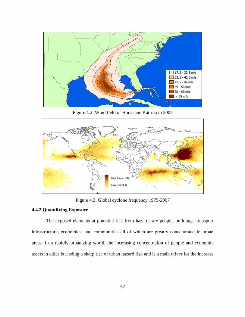
57
Figure 4.2: Wind field of Hurricane Katrina in 2005
Figure 4.3: Global cyclone frequency 1975-2007
4.4.2 Quantifying Exposure
The exposed elements at potential risk from hazards are people, buildings, transport
infrastructure, economies, and communities all of which are greatly concentrated in urban
areas. In a rapidly urbanizing world, the increasing concentration of people and economic
assets in cities is leading a sharp rise of urban hazard risk and is a main driver for the increase
High (count 74)
Low (count 1)
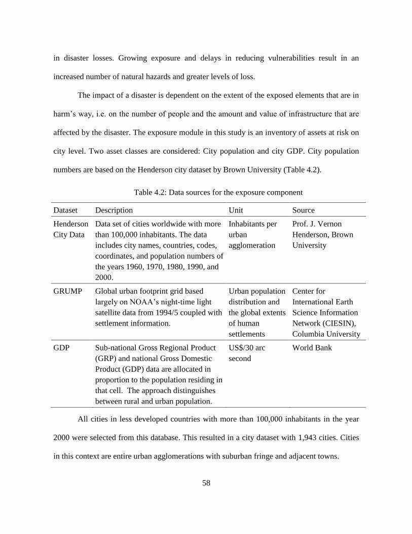
58
in disaster losses. Growing exposure and delays in reducing vulnerabilities result in an
increased number of natural hazards and greater levels of loss.
The impact of a disaster is dependent on the extent of the exposed elements that are in
harm’s way, i.e. on the number of people and the amount and value of infrastructure that are
affected by the disaster. The exposure module in this study is an inventory of assets at risk on
city level. Two asset classes are considered: City population and city GDP. City population
numbers are based on the Henderson city dataset by Brown University (Table 4.2).
Table 4.2: Data sources for the exposure component
Dataset Description Unit Source
Henderson
City Data
Data set of cities worldwide with more
than 100,000 inhabitants. The data
includes city names, countries, codes,
coordinates, and population numbers of
the years 1960, 1970, 1980, 1990, and
2000.
Inhabitants per
urban
agglomeration
Prof. J. Vernon
Henderson, Brown
University
GRUMP Global urban footprint grid based
largely on NOAA’s night-time light
satellite data from 1994/5 coupled with
settlement information.
Urban population
distribution and
the global extents
of human
settlements
Center for
International Earth
Science Information
Network (CIESIN),
Columbia University
GDP Sub-national Gross Regional Product
(GRP) and national Gross Domestic
Product (GDP) data are allocated in
proportion to the population residing in
that cell. The approach distinguishes
between rural and urban population.
US$/30 arc
second
World Bank
All cities in less developed countries with more than 100,000 inhabitants in the year
2000 were selected from this database. This resulted in a city dataset with 1,943 cities. Cities
in this context are entire urban agglomerations with suburban fringe and adjacent towns.
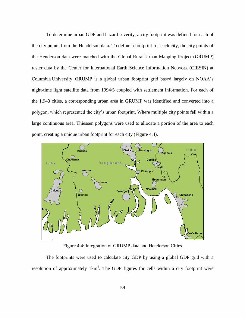
59
To determine urban GDP and hazard severity, a city footprint was defined for each of
the city points from the Henderson data. To define a footprint for each city, the city points of
the Henderson data were matched with the Global Rural-Urban Mapping Project (GRUMP)
raster data by the Center for International Earth Science Information Network (CIESIN) at
Columbia University. GRUMP is a global urban footprint grid based largely on NOAA’s
night-time light satellite data from 1994/5 coupled with settlement information. For each of
the 1,943 cities, a corresponding urban area in GRUMP was identified and converted into a
polygon, which represented the city’s urban footprint. Where multiple city points fell within a
large continuous area, Thiessen polygons were used to allocate a portion of the area to each
point, creating a unique urban footprint for each city (Figure 4.4).
Figure 4.4: Integration of GRUMP data and Henderson Cities
The footprints were used to calculate city GDP by using a global GDP grid with a
resolution of approximately 1km2. The GDP figures for cells within a city footprint were
60
added up which resulted in the city GDP. By overlying the footprints with the natural hazard
grids, the footprints were the basis for identifying if a city was exposed to natural hazards, and
if so, to what maximum hazard probability.
4.4.3 Calculating Vulnerability
The term ‘vulnerability’ is derived from the Latin word vulnerare, which means 'to
wound'. Broadly, vulnerability refers to the extent to which a person, structure, or service is
likely to be damaged by the impact of a disaster. It explains why, with a given hazard
severity, people and assets are more or less at risk and why they do or do not fail to be robust
in the face of a threatening event. For the purpose of a risk assessment, vulnerability is usually
disaggregated into categories such as physical, social, economic, or environmental. While
physical vulnerability of the built environment, for example, is influenced by building age and
construction type, social vulnerability is affected by lack of access to resources or limited
access to political power.
Vulnerability reduction is a core element in disaster risk management. The concept of
vulnerability has helped to highlight the role of social and physical factors that have an impact
on the constitution of risk (Hewitt 1983). By using the notion of vulnerability, disasters are
not viewed anymore only as the result of a natural event but rather as the result of the
vulnerability of a society, its infrastructure, economy, and environment, all of which are
determined by human behavior. Governments and citizens can appreciably reduce
vulnerability, and therefore risk, through sensible combinations of prevention, insurance, and
preparedness.
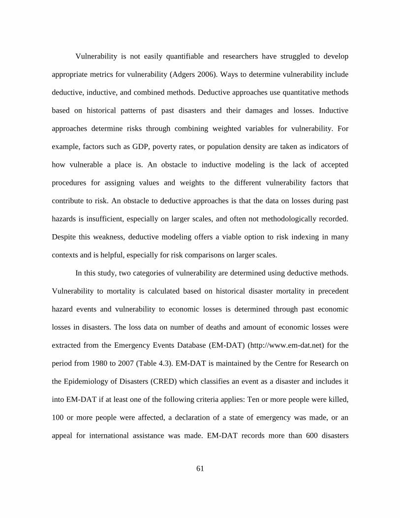
61
Vulnerability is not easily quantifiable and researchers have struggled to develop
appropriate metrics for vulnerability (Adgers 2006). Ways to determine vulnerability include
deductive, inductive, and combined methods. Deductive approaches use quantitative methods
based on historical patterns of past disasters and their damages and losses. Inductive
approaches determine risks through combining weighted variables for vulnerability. For
example, factors such as GDP, poverty rates, or population density are taken as indicators of
how vulnerable a place is. An obstacle to inductive modeling is the lack of accepted
procedures for assigning values and weights to the different vulnerability factors that
contribute to risk. An obstacle to deductive approaches is that the data on losses during past
hazards is insufficient, especially on larger scales, and often not methodologically recorded.
Despite this weakness, deductive modeling offers a viable option to risk indexing in many
contexts and is helpful, especially for risk comparisons on larger scales.
In this study, two categories of vulnerability are determined using deductive methods.
Vulnerability to mortality is calculated based on historical disaster mortality in precedent
hazard events and vulnerability to economic losses is determined through past economic
losses in disasters. The loss data on number of deaths and amount of economic losses were
extracted from the Emergency Events Database (EM-DAT) (http://www.em-dat.net) for the
period from 1980 to 2007 (Table 4.3). EM-DAT is maintained by the Centre for Research on
the Epidemiology of Disasters (CRED) which classifies an event as a disaster and includes it
into EM-DAT if at least one of the following criteria applies: Ten or more people were killed,
100 or more people were affected, a declaration of a state of emergency was made, or an
appeal for international assistance was made. EM-DAT records more than 600 disasters
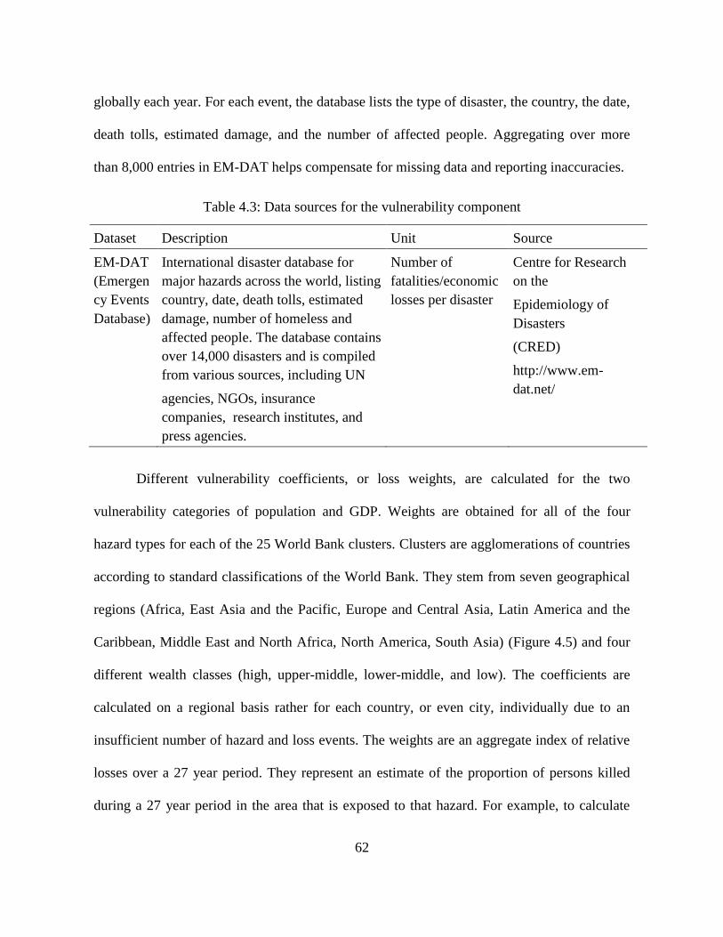
62
globally each year. For each event, the database lists the type of disaster, the country, the date,
death tolls, estimated damage, and the number of affected people. Aggregating over more
than 8,000 entries in EM-DAT helps compensate for missing data and reporting inaccuracies.
Table 4.3: Data sources for the vulnerability component
Dataset Description Unit Source
EM-DAT
(Emergen
cy Events
Database)
International disaster database for
major hazards across the world, listing
country, date, death tolls, estimated
damage, number of homeless and
affected people. The database contains
over 14,000 disasters and is compiled
from various sources, including UN
agencies, NGOs, insurance
companies, research institutes, and
press agencies.
Number of
fatalities/economic
losses per disaster
Centre for Research
on the
Epidemiology of
Disasters
(CRED)
http://www.em-
dat.net/
Different vulnerability coefficients, or loss weights, are calculated for the two
vulnerability categories of population and GDP. Weights are obtained for all of the four
hazard types for each of the 25 World Bank clusters. Clusters are agglomerations of countries
according to standard classifications of the World Bank. They stem from seven geographical
regions (Africa, East Asia and the Pacific, Europe and Central Asia, Latin America and the
Caribbean, Middle East and North Africa, North America, South Asia) (Figure 4.5) and four
different wealth classes (high, upper-middle, lower-middle, and low). The coefficients are
calculated on a regional basis rather for each country, or even city, individually due to an
insufficient number of hazard and loss events. The weights are an aggregate index of relative
losses over a 27 year period. They represent an estimate of the proportion of persons killed
during a 27 year period in the area that is exposed to that hazard. For example, to calculate
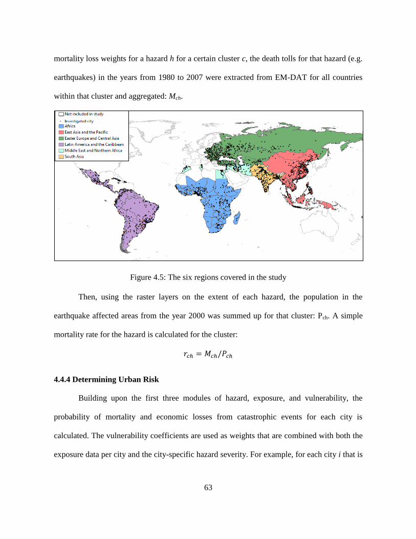
63
mortality loss weights for a hazard h for a certain cluster c, the death tolls for that hazard (e.g.
earthquakes) in the years from 1980 to 2007 were extracted from EM-DAT for all countries
within that cluster and aggregated: Mch.
Figure 4.5: The six regions covered in the study
Then, using the raster layers on the extent of each hazard, the population in the
earthquake affected areas from the year 2000 was summed up for that cluster: Pch. A simple
mortality rate for the hazard is calculated for the cluster:
4.4.4 Determining Urban Risk
Building upon the first three modules of hazard, exposure, and vulnerability, the
probability of mortality and economic losses from catastrophic events for each city is
calculated. The vulnerability coefficients are used as weights that are combined with both the
exposure data per city and the city-specific hazard severity. For example, for each city i that is
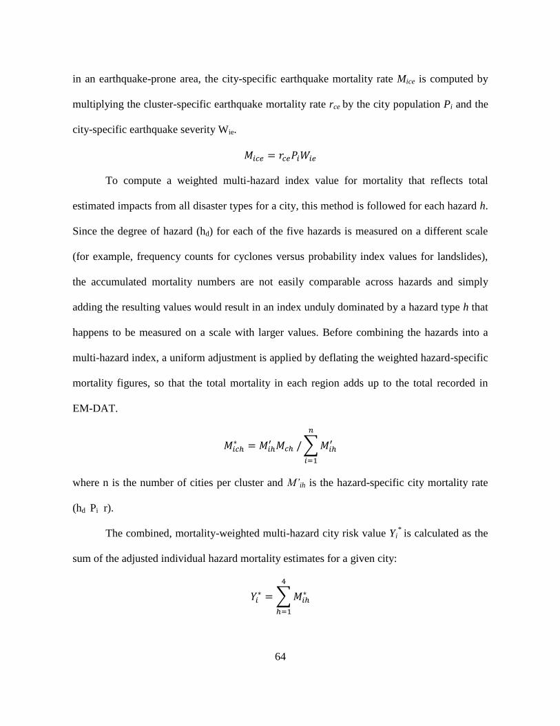
64
in an earthquake-prone area, the city-specific earthquake mortality rate Mice is computed by
multiplying the cluster-specific earthquake mortality rate rce by the city population Pi and the
city-specific earthquake severity Wie.
To compute a weighted multi-hazard index value for mortality that reflects total
estimated impacts from all disaster types for a city, this method is followed for each hazard h.
Since the degree of hazard (hd) for each of the five hazards is measured on a different scale
(for example, frequency counts for cyclones versus probability index values for landslides),
the accumulated mortality numbers are not easily comparable across hazards and simply
adding the resulting values would result in an index unduly dominated by a hazard type h that
happens to be measured on a scale with larger values. Before combining the hazards into a
multi-hazard index, a uniform adjustment is applied by deflating the weighted hazard-specific
mortality figures, so that the total mortality in each region adds up to the total recorded in
EM-DAT.
∑
where n is the number of cities per cluster and M’ih is the hazard-specific city mortality rate
(hd Pi r).
The combined, mortality-weighted multi-hazard city risk value Yi*
is calculated as the
sum of the adjusted individual hazard mortality estimates for a given city:
∑
65
Reporting actual mortality numbers would portray an unrealistic impression of
precision. To avoid literal interpretation of the disaster index as the number of persons
expected to be killed in a 20-year period and in recognition of the many limitations of the
underlying data, the resulting measures are converted into index values from one to ten,
classifying the global risk distribution into deciles and providing relative presentations of
disaster risk.
4.4.5 Interpretation
The calculated risks in the index assign a value to the city as a whole and are based on
the three factors of hazard severity in the city, city population, and the vulnerability of the
particular World Bank cluster. The mortality risk in a city is the potential extent of total
fatality numbers that a city could incur rather than the extent of risk that a single person
experiences in that city. Similarly, economic risk mirrors total potential damage extent.
Result interpretation needs to consider that a number of constraints in globally
available data limit the sophistication of the methods that were employed to investigate urban
risk on a global level. Although I use the best available data, gaps in the data limit our
analysis. For example, deductive modeling has weaknesses in determining risk in contexts
where disasters occur infrequently and where historical data is scarce. Moreover, disaster loss
data in EM-DAT is recorded on country-level and does not allow for a differentiation between
urban and rural loss rates and vulnerabilities. The insufficient numbers of disaster events lead
us to calculate vulnerability coefficients on regional levels using clusters. Aggregating across
more than 8,000 entries in EM-DAT helps compensate for missing data and inaccuracies and
reflect broad patterns of vulnerability. It cannot, however, reveal protection mechanisms (land

66
use planning, regulations) that individual cities might have implemented. Another limiting
factor is the relatively crude delineation of some hazards. For example, earthquakes with
pathological damage patterns are represented incompletely. The cities investigated in this
study stem from the Henderson city database (see Table 4.2). This data set contains cities
worldwide with more than 100,000 inhabitants. While it has extensive coverage globally,
some cities are left out in the database and are consequently not included in the index. Finally,
for a few clusters (i.e. Middle East and Northern Africa High Income, Middle East and
Northern Africa Lower Middle Income, all clusters in the Africa region, and Eastern Europe
and Central Asia Lower Middle Income) insufficient historic loss data was available for
landslide hazards, and therefore, the countries belonging to those clusters were not included in
the landslide analysis.
In recognition of these limitations, the modest objective of the study is to provide a
relative presentation of disaster risk instead of an absolute one. We therefore convert the
absolute city risk values, calculated in the risk model, into comparative index values. While
the index cannot provide the detail needed to identify concrete risk reduction measures, it
assesses the relative importance of risk at regional level and identifies areas where more
attention is needed.
4.5 Results
Global Distribution
The number of exposed urban dwellers to certain hazards has implications for the
weight given to reduce the risk of specific hazards. In this analysis, by far the greatest number
of the investigated urban population in less developed countries is exposed to flood hazards,
67
approximately 1.1 billion. Around half that number (560 million) are at risk to earthquakes
and also to landslides (660 million). Finally, nearly 90 million of the study’s urban population
is exposed to cyclone hazards.
Regional Distribution
Between 1980 and 2006, Pakistan and the US both experienced nineteen major
earthquakes (>5.0 on Richter scale). While in Pakistan 74,112 people died during these
earthquakes, in the US only 145 people were killed. This enforces the concept that tragedies
are not caused by the earthquake itself, but rather by dire construction practices and missing
policies. The deaths and devastation in disasters result from human action or inaction.
Typically, wealthy regions and countries are higher at risk in terms of economic losses but
suffer fewer fatalities whereas poor countries experience high mortality risks and lesser
economic risks. The results in Figure 4.6 reflect this trend. This figure shows the accumulated
shares of urban economic and mortality risks by region and hazard. Within the individual
regions, significant differences can be found in terms risks to mortality and economic loss
risks. For example, while urban mortality loss risk to cyclones is greatest in South Asia
(68%), the share of urban cyclone economic loss risk in the same region is only 16%. The
wealthier East Asia clearly bears the greatest burden of urban economic loss risk (77%)
whereas East Asia’s urban mortality risk is comparatively lower. Next to wealth, the type of
disaster is a decisive factor for overall risk. Fatalities from severe earthquakes, for example,
are usually far larger than fatalities from severe floods or cyclones under equal vulnerability
conditions.

68
Earthquake mortality risk Earthquake economic loss risk
Cyclone mortality risk Cyclone economic loss risk
Landslide mortality risk Landslide economic loss risk
Flood mortality risk Flood economic loss risk
Figure 4.6: Regional shares of urban risks for four different hazards
0% 4%
35%
5%
28%
28%
0% 5%
60% 9%
19%
7%
1%
22%
0% 9%
0% 68%
4%
77%
0%
3% 0% 16%
2%
28%
31%
19%
1% 19% 13%
76%
11%
28%
25%
2%
20%
3%
22% 39%
44%
5%
5% 1% 6%
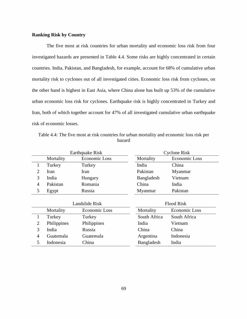
69
Ranking Risk by Country
The five most at risk countries for urban mortality and economic loss risk from four
investigated hazards are presented in Table 4.4. Some risks are highly concentrated in certain
countries. India, Pakistan, and Bangladesh, for example, account for 68% of cumulative urban
mortality risk to cyclones out of all investigated cities. Economic loss risk from cyclones, on
the other hand is highest in East Asia, where China alone has built up 53% of the cumulative
urban economic loss risk for cyclones. Earthquake risk is highly concentrated in Turkey and
Iran, both of which together account for 47% of all investigated cumulative urban earthquake
risk of economic losses.
Table 4.4: The five most at risk countries for urban mortality and economic loss risk per
hazard
Earthquake Risk
Cyclone Risk
Mortality Economic Loss
Mortality Economic Loss
1 Turkey Turkey
India China
2 Iran Iran
Pakistan Myanmar
3 India Hungary
Bangladesh Vietnam
4 Pakistan Romania
China India
5 Egypt Russia
Myanmar Pakistan
Landslide Risk
Flood Risk
Mortality Economic Loss
Mortality Economic Loss
1 Turkey Turkey
South Africa South Africa
2 Philippines Philippines
India Vietnam
3 India Russia
China China
4 Guatemala Guatemala
Argentina Indonesia
5 Indonesia China
Bangladesh India

70
Ranking Risks by City
The cities with the highest mortality and economic loss risk by hazard are listed in
Table 4.5 to Table 4.8. The tables show the five most at risk cities by hazard in each of the six
investigated regions. The ranking gives an indication of the cities most worthy of further and
more detailed investigation. The data provide for interesting comparisons. For example,
Metro Manila, one of the world’s most disaster prone cities, is listed in the tables as being
highly at risks from the three hazards of earthquakes, floods and landslides. This year, in
2012, the city has again experienced devastating floods with almost two thirds of the city area
being submerged after a week of torrential rains. Tehran is also highly at risk, especially from
earthquakes and floods. This fact has sparked repeated discussions among the country’s
leaders about moving the capital to a less risky region. A striking, but also sobering, result is
the magnitude of risk in certain cities. In South Asia, the top five ranked cities for cyclone
mortality risk bear 62% of all cumulative mortality loss risk in that region. Cumulative
economic loss risk for landslides in Eastern Europe and Central Asia amounts to 51% for the
top five ranked cities in that category. All of those five cities are in Turkey. In Africa, Addis
Ababa accounts for 31% of the cumulative earthquake mortality risk in that region and the top
five cities altogether bear 59% of Africa’s earthquake mortality risk.
A number of smaller cities with less population and wealth are set to swell with rapid
increases in population and asset exposure. These include, for example, Toluca in Mexico and
Conakry in Guinea. While the absolute exposure of these cities is currently relatively low, the
rapid increase in population growth will pose significant challenges for these cities in the
coming years.

71
Table 4.5: Regional top 5 cities most at risk to earthquakes
Mortality risk Economic loss risk
Region Country City Country City
Africa Ethiopia Addis Ababa Uganda Kampala
Uganda Kampala Ethiopia Addis Ababa
Malawi Blantyre Malawi Blantyre
Kenya Nakuru Kenya Kisumu
Burundi Bujumbura Kenya Nakuru
East Asia Philippines Metro Manila Indonesia Jakarta
Indonesia Jakarta Philippines Metro Manila
China Tianjin China Beijing
China Beijing China Tianjin
Indonesia Bandung Indonesia Yogyakarta
Eastern
Europe and
Central Asia
Turkey Istanbul Turkey Ankara
Turkey Ankara Hungary Budapest
Turkey Izmir Turkey Izmit
Romania Bucharest Turkey Istanbul
Turkey Bursa Turkey Izmir
Latin
America and
the
Caribbean
Mexico Mexico City Peru Lima
Peru Lima Mexico Mexico City
Chile Santiago Mexico Tijuana
Colombia Bogota Colombia Bogota
Mexico Guadalajara Chile Santiago
Middle East
and
Northern
Africa
Egypt Cairo Iran Tehran
Iran Tehran Egypt Cairo
Iran Mashhad Iran Raja'ishahr
Iran Esfahan Egypt Shubra El-Kheima
Tunisia Tunis Iran Ahvaz
South Asia India Kolkata India Delhi
Bangladesh Dhaka India Kolkata
Pakistan Karachi Pakistan Karachi
India Delhi Pakistan Lahore
Pakistan Lahore Bangladesh Dhaka
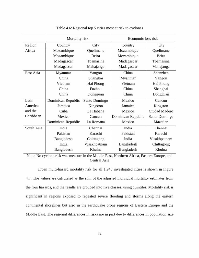
72
Table 4.6: Regional top 5 cities most at risk to cyclones
Mortality risk Economic loss risk
Region Country City Country City
Africa Mozambique Quelimane Mozambique Quelimane
Mozambique Beira Mozambique Beira
Madagascar Toamasina Madagascar Toamasina
Madagascar Mahajanga Madagascar Mahajanga
East Asia Myanmar Yangon China Shenzhen
China Shanghai Myanmar Yangon
Vietnam Hai Phong Vietnam Hai Phong
China Fuzhou China Shanghai
China Dongguan China Dongguan
Latin
America
and the
Caribbean
Dominican Republic Santo Domingo Mexico Cancun
Jamaica Kingston Jamaica Kingston
Cuba La Habana Mexico Ciudad Madero
Mexico Cancun Dominican Republic Santo Domingo
Dominican Republic La Romana Mexico Mazatlan
South Asia India Chennai India Chennai
Pakistan Karachi Pakistan Karachi
Bangladesh Chittagong India Visakhpatnam
India Visakhpatnam Bangladesh Chittagong
Bangladesh Khulna Bangladesh Khulna
Note: No cyclone risk was measure in the Middle East, Northern Africa, Eastern Europe, and
Central Asia
Urban multi-hazard mortality risk for all 1,943 investigated cities is shown in Figure
4.7. The values are calculated as the sum of the adjusted individual mortality estimates from
the four hazards, and the results are grouped into five classes, using quintiles. Mortality risk is
significant in regions exposed to repeated severe flooding and storms along the eastern
continental shorelines but also in the earthquake prone regions of Eastern Europe and the
Middle East. The regional differences in risks are in part due to differences in population size

73
Table 4.7: Regional top 5 cities most at risk to landslides
Mortality risk Economic loss risk
Region Country City Country City
Africa Sierra Leone Freetown
Guinea Conakry
Nigeria Lagos
Côte d'Ivoire Abidjan
Ethiopia Adis Abeba
East Asia Philippines Metro Manila Philippines Metro Manila
Indonesia Surabaya China Shenzhen
Philippines Baguio Indonesia Surabaya
Vietnam Ho Chi Minh Indonesia Yogyakarta
Indonesia Padang China Hong Kong
Eastern
Europe
and
Central
Asia
Turkey Manisa Turkey Izmit
Turkey Izmir Turkey Manisa
Russia Petropavlovsk-Kamatskij Turkey Kahramanmaras
Turkey Kahramanmaras Turkey Izmir
Turkey Erzurum Turkey Erzurum
Latin
America
and the
Caribbean
Guatemala Guatemala City Guatemala Guatemala City
Ecuador Quito Brazil Vitoria
Colombia Bogota Peru Lima
Peru Lima Ecuador Quito
Brazil Vitoria El Salvador San Salvador
Middle
East and
Northern
Africa
Iran Tehran Bahrain Al-Manamah
Iran Rasht Djibouti Djibouti
Iran Shiraz Iran Tehran
Iran Tabriz Iran Mashhad
Iran Khorramabad Iran Esfahan
South
Asia
India Imphal India Imphal
India Mumbai India Srinagar
India Srinagar India Thane
Pakistan Peshawar India Bhiwandi
Pakistan Islamabad India Chandigarh
Note: Due to lack of data, economic loss risk for landslides could not be calculated in Africa.
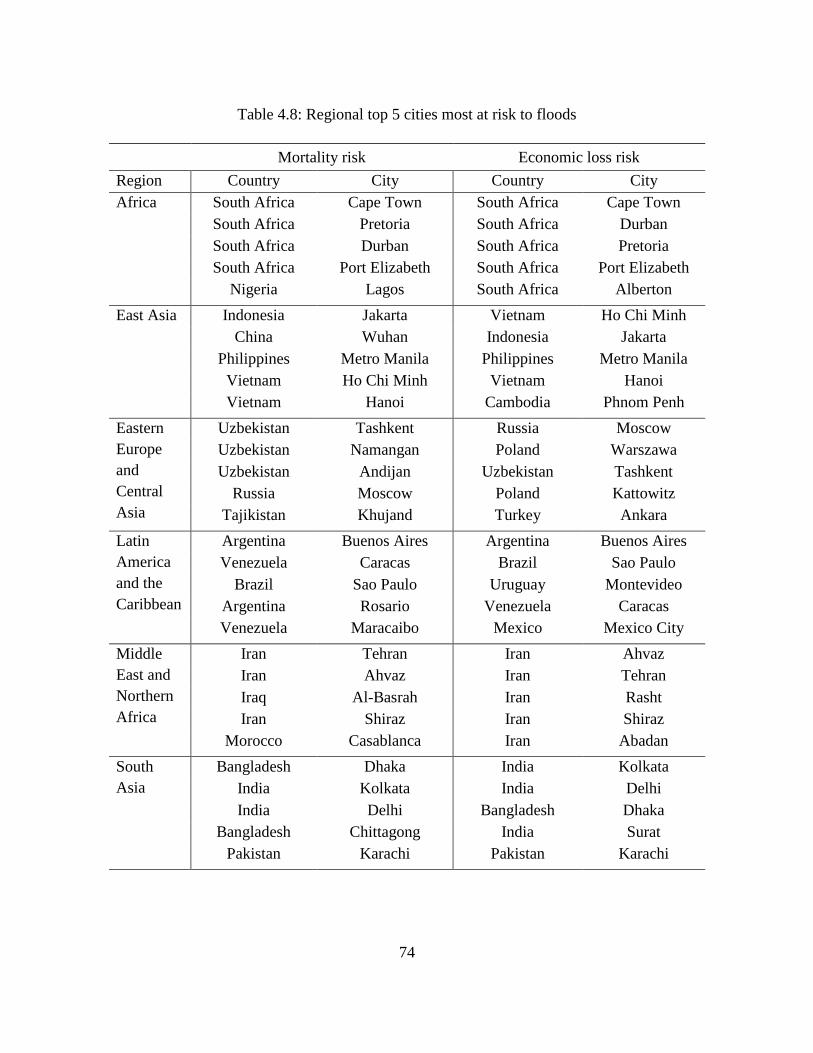
74
Table 4.8: Regional top 5 cities most at risk to floods
Mortality risk Economic loss risk
Region Country City Country City
Africa South Africa Cape Town South Africa Cape Town
South Africa Pretoria South Africa Durban
South Africa Durban South Africa Pretoria
South Africa Port Elizabeth South Africa Port Elizabeth
Nigeria Lagos South Africa Alberton
East Asia Indonesia Jakarta Vietnam Ho Chi Minh
China Wuhan Indonesia Jakarta
Philippines Metro Manila Philippines Metro Manila
Vietnam Ho Chi Minh Vietnam Hanoi
Vietnam Hanoi Cambodia Phnom Penh
Eastern
Europe
and
Central
Asia
Uzbekistan Tashkent Russia Moscow
Uzbekistan Namangan Poland Warszawa
Uzbekistan Andijan Uzbekistan Tashkent
Russia Moscow Poland Kattowitz
Tajikistan Khujand Turkey Ankara
Latin
America
and the
Caribbean
Argentina Buenos Aires Argentina Buenos Aires
Venezuela Caracas Brazil Sao Paulo
Brazil Sao Paulo Uruguay Montevideo
Argentina Rosario Venezuela Caracas
Venezuela Maracaibo Mexico Mexico City
Middle
East and
Northern
Africa
Iran Tehran Iran Ahvaz
Iran Ahvaz Iran Tehran
Iraq Al-Basrah Iran Rasht
Iran Shiraz Iran Shiraz
Morocco Casablanca Iran Abadan
South
Asia
Bangladesh Dhaka India Kolkata
India Kolkata India Delhi
India Delhi Bangladesh Dhaka
Bangladesh Chittagong India Surat
Pakistan Karachi Pakistan Karachi

75
but also the degree of hazard severity and frequency across regions. Additionally, the
differences reflect the variation in vulnerability. Similarly, economic risk is shown on Figure
4.8.
Figure 4.7: Urban mortality risk
Figure 4.8: Urban economic loss risk
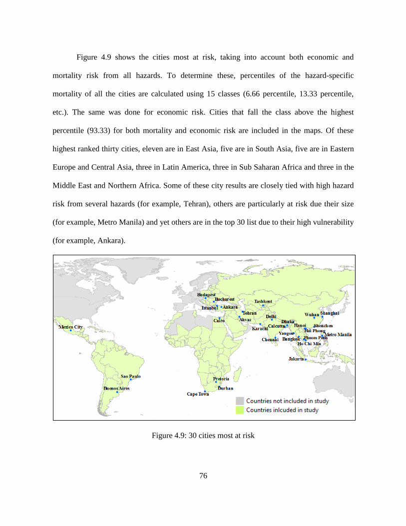
76
Figure 4.9 shows the cities most at risk, taking into account both economic and
mortality risk from all hazards. To determine these, percentiles of the hazard-specific
mortality of all the cities are calculated using 15 classes (6.66 percentile, 13.33 percentile,
etc.). The same was done for economic risk. Cities that fall the class above the highest
percentile (93.33) for both mortality and economic risk are included in the maps. Of these
highest ranked thirty cities, eleven are in East Asia, five are in South Asia, five are in Eastern
Europe and Central Asia, three in Latin America, three in Sub Saharan Africa and three in the
Middle East and Northern Africa. Some of these city results are closely tied with high hazard
risk from several hazards (for example, Tehran), others are particularly at risk due their size
(for example, Metro Manila) and yet others are in the top 30 list due to their high vulnerability
(for example, Ankara).
Figure 4.9: 30 cities most at risk
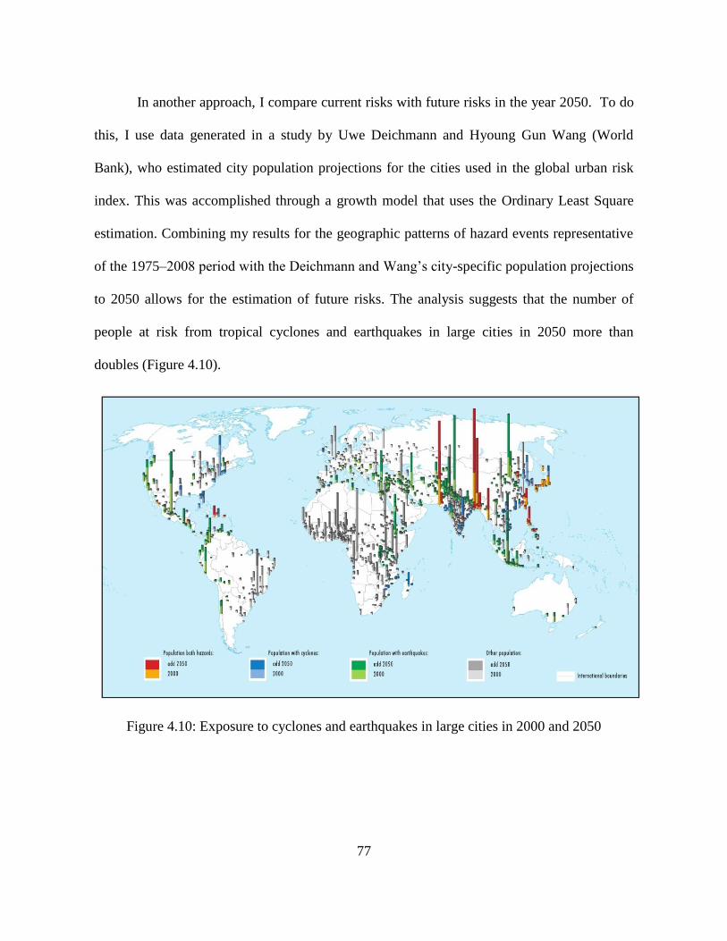
77
In another approach, I compare current risks with future risks in the year 2050. To do
this, I use data generated in a study by Uwe Deichmann and Hyoung Gun Wang (World
Bank), who estimated city population projections for the cities used in the global urban risk
index. This was accomplished through a growth model that uses the Ordinary Least Square
estimation. Combining my results for the geographic patterns of hazard events representative
of the 1975–2008 period with the Deichmann and Wang’s city-specific population projections
to 2050 allows for the estimation of future risks. The analysis suggests that the number of
people at risk from tropical cyclones and earthquakes in large cities in 2050 more than
doubles (Figure 4.10).
Figure 4.10: Exposure to cyclones and earthquakes in large cities in 2000 and 2050
78
4.6 Sensitivity Analysis
Sensitivity analysis, applied to a risk assessment, is a method used to understand how
risk estimates depend on the variability and uncertainty of the factors used in the analysis. It
determines how the different factors used in the index construction process affect the outputs,
and it plays an important role in the verification and validation of the model. According to
Saltelli at al. (2000) a sensitivity analysis is conducted to determine, for example, a) if the
model resembles the system under study; b) the factors that most influence the output
variability and therefore require special attention; c) the model parameters that are
insignificant and that can be omitted; and d) which factors interact with each other. It is the
final step in index development analysis, which examines the sensitivity of the model to
changes in its inputs, and that gives an indication on the level of confidence or uncertainty. In
existing risk and vulnerability indices, this last step has often been omitted.
In the Urban Risk Index, sources of uncertainties include: a) the underlying hazard
models, b) the delineation of cities, c) the global grids for GDP and population, and d) the
vulnerability coefficients. Future work on the index could conduct local sensitivity analysis by
varying these input factors one at a time and examine the impact, while the other factors
remain constant. Since the index measures relative values, the sensitivity of the relative, not
absolute, values would need to be examined. These analyses could be developed for the
individual four single hazard indices.
For the multi-hazard index, which simply adds the values of the single hazard indices,
it would be interesting to determine which of the four indices have the largest influence in the
overall urban multi-hazard risk. The percentage values to which the single hazard indices
79
contribute to the overall index vary largely from 0-100% for all four hazards. A preliminary
analysis was carried that investigates how the top 20 cities of the multi-hazard mortality index
change if one single hazard value is removed. If the landslide results are omitted from the
overall index, only one city out of the top 20 cities changes. If the flood index values are
omitted, three cities change in the top 20. Removing the cyclones from the overall index,
results in a change of six cities and, finally, excluding earthquakes results in a change of
seven cities in the top 20 cities. This corresponds to the fact that earthquakes, on average,
cause large fatality numbers.
4.7 Conclusion
This study assesses the risk of mortality and economic loss from catastrophic events in
cities of less developed countries worldwide with a population greater than 100,000. Risk is
calculated by combining the three modules of hazard, exposure, and vulnerability. The urban
hazards are determined by overlaying the city locations with hazard severity grids; regional
vulnerability coefficients are based on loss data from past events; and exposure is defined
through city population and city GDP. Four single hazard risk indices are developed and in
addition, a multi-hazard index gives a holistic picture of city risk. The absolute risk values are
converted into index values, classifying the results into relative presentations of risk.
Expected urban risk exposure in the year 2050 is determined through projections of future city
population growth.
By revealing risk levels, I hope to contribute to the knowledge on the variation of
urban risks. Such knowledge is useful for local and national planners, as well as international
donors. Disclosing risks to cities raises awareness, informs the prioritization of resources,
80
inspires further research, particularly at local levels, and promotes a shift towards managing
risks rather than emergencies.
The index also provides a baseline for channeling international interest and funding
for detailed urban multi-hazard risk assessments. These detailed assessments of the hazards,
elements at risks, and the present vulnerabilities are required to gain a deep understanding for
effective risk reduction and financial risk transfer mechanisms. Once the underlying risks in a
city are known, the key drivers of risk can be addressed through a range of policy options, for
instance, through building codes, environmental rehabilitation, land use planning, and early
warning. Since the current lack of integration of urban development and risk reduction
increases vulnerabilities and expected future losses, a shift to proactive and preventive urban
planning underpinned with the principle of diminishing risk is needed. This increased role of
urban planning as a tool for reducing disaster is perhaps the most important public policy
recommendation from this paper.
4.8 References
Adger, W. N. (2006). Vulnerability. Global Environmental Change, 16(3): 268-281.
Angel S., S. Sheppard S. & D. Civco (2005). The Dynamics of Global Urban Expansion.
Transport and Urban Development Department, World Bank, Washington DC.
Arnold, M. & A. Kreimer (2004). The socio-economic costs of disasters. In An Adaptation
Mosaic: An Example of Emerging Bank Work in Climate Change Adaptation, eds.
Mathur A., I. Burton and M. van Aalst, 5-15. Washington, DC: World Bank.
Association of Southeast Asian Nations (ASEAN) (2010): ASEAN Agreement on Disaster
Management and Emergency Response - Work programme for 2010-2015: Building
disaster-resilient nations and safer communities. Jakarta: ASEAN.
81
Ashdown, L. (2011). Humanitarian Emergency Response Review (HERR). London:
Department for International Development (DFID). [Retrieved from
www.dfid.gov.uk/emergency-response-review].
Bengtsson, L., K.I. Hodges & E. Roeckner (2006). Storm tracks and climate change. Journal
of Climate, 19: 3518-3543.
Birkmann, J. (2006). Measuring vulnerability to promote disaster-resilient societies:
conceptual frameworks and definitions. In Measuring Vulnerability to Natural
Hazards: Towards Disaster Resilient Societies, ed. Birkmann, J., 9-54. Tokyo: United
Nations University Press.
Blaikie, P., T. Cannon, I. Davis & B. Wisner (1994). At Risk: Natural Hazards, People’s
Vulnerability and Disasters. London: Routledge.
Brecht, H., S. Dasgupta, B. Laplante, S. Murray, and D. Wheeler (2012). Sea-level rise and
storm surges: High stakes for a small number of developing countries. The Journal of
Environment Development, 21(1): 102-138.
Cardona, O. (2005). Indicators of Disaster Risk and Risk Management: Program for Latin
America and the Carribean. Main Technical Report. Washington, DC: Inter-American
Development Bank (IDB).
Cutter, S. (ed.) (2001). American Hazardscapes: the Regionalization of Hazards and
Disasters. Washington, DC: Joseph Henry Press.
Cutter, S.L. & C. Finch (2008). Temporal and spatial changes in social vulnerability to natural
hazards. Proceedings of the National Academy of Sciences, 105(7): 2301-2306.
Davidson, R. (1997). A multidisciplinary urban earthquake disaster risk index. Earthquake
Spectra, 13(2): 211–223.
Dilley, M., R. Chen, U. Deichmann, A. Lerner-Lam, M. Arnold, J. Agwe, P. Buys, O.
Kjekstad, B. Lyon & G. Yetman (2005). Natural Disaster Hotspots: A Global
Analysis. World Bank Disaster Risk Management Series, No. 5. Washington, DC:
World Bank.
Emanuel, K. (2005). Increasing destructiveness of tropical cyclones over the past 30 years.
Nature, 436: 686–688.
Füssel, H.-M. (2007). Vulnerability: A generally applicable conceptual framework for climate
change research. Global Environmental Change, 17: 155-167.

82
Gill, I. & H. Kharas (2007). An East Asian Renaissance: Ideas for Economic Growth.
Washington, DC: World Bank.
Hanson, S., R. Nicholls, N. Ranger, S. Hallegatte, J. Corfee-Morlot, C. Herweijer & J.
Chateau (2011). A global ranking of port cities with high exposure to climate
extremes. Climatic Change, 104: 89-111.
Hewitt, K. (ed.) (1983). Interpretation of Calamity: From the Viewpoint of Human Ecology.
Boston: Allen & Unwin.
Lerner-Lam, A. (2007). Assessing global exposure to natural hazards: Progress and future
trends. Environmental Hazards, 7(1): 10–19.
McGranahan, G., D. Balk & B. Anderson (2007). The rising tide: assessing the risks of
climate change and human settlements in low elevation coastal zones. Environment
and Urbanization, 19(1): 17-37.
Mileti, D. (1999). Disasters by Design. Washington, DC : Joseph Henry Press.
Munich Re (2003a). Annual Review: Natural Catastrophes 2002, Topics. Munich: Author.
[Retrieved from http://www.munichre.com/publications/302-03631_en.pdf?
rdm=75077].
Peduzzi, P., H. Dao, C. Herold & F. Mouton. (2009). Assessing global exposure and
vulnerability towards natural hazards: the Disaster Risk Index. Natural Hazards and
Earth System Sciences, 9: 1149-1159.
Pelling, M. (2003). The Vulnerability of Cities: Social Resilience and Natural Disaster.
London: Earthscan.
Plate, E. J. (2002). Flood risk and flood management. Journal of Hydrology, 267(1): 2–11.
Saltelli, A., K. Chan, and E. M. Scott (eds.) (2000). Sensitivity Analysis, Wiley Series in
Probability and Statistics. New York: John Wiley & Sons, Ltd.
Smith, K. (1996). Environmental Hazards: Assessing Risk and Reducing Disaster, 2nd
edn.
London: Routledge.
Tierney, K. (2002). Methods of Disaster Research, Xlibris Corporation, chapter The Field
Turns Fifty: Social Change and the Practice of Disaster Fieldwork, pp. 349–374.
UN (2008). World Urbanization Prospects 2007 Revision, United Nations Population
Division, New York.

83
UN-ISDR (2005). Hyogo Framework for Action 2005-2015: Building the Resilience of
Nations and Communities to Disasters, United Nations International Strategy for
Disaster Risk Reduction, Geneva.
UN-ISDR (2009). Global Assessment Report on Disaster Risk Reduction: Invest Today for a
Safer Tomorrow, United Nations, Geneva, Switzerland.
UN-ISDR (20011). Global Assessment Report on Disaster Risk Reduction: Revealing Risks,
Redefining Development, United Nations, Geneva, Switzerland.
Vermeer, M. & S. Rahmstorf (2009). Global sea level linked to global temperature.
Proceedings of the National Academy of Sciences, 106: 21527-21532.
White, G.F. (1973). Natural hazards research. In Directions in Geography, ed. R.J. Chorley,
193-216. London: Methuen.
Wisner, B. (2003). Building Safer Cities: The Future of Disaster Risk. In Disaster Risk
Reduction in Megacities: Making the Most of Human and Social Capital. World Bank
Disaster Risk Management Series, No. 3, 181–196. Washington, DC: The World
Bank.
World Bank (2006). Hazards of Nature, Risks to Development: An IEG Evaluation of World
Bank Assistance for Natural Disaster. Washington, DC: World Bank.
World Bank (2009). Reshaping Economic Geography. World Development Report 2009.
Washington DC: World Bank.
World Bank (2010). Climate Risks and Adaptation in Asian Coastal Megacities. Washington,
DC: World Bank.
84
CHAPTER 5 : SEA-LEVEL RISE AND STORM SURGES:IGH STAKES FOR A
SEA-LEVEL RISE AND STORM SURGES: HIGH STAKES FOR A SMALL
NUMBER OF DEVELOPING COUNTRIES3
5.1 Introduction
Large tropical cyclones create storm surges that can strike crowded coastal regions
with devastating force. During the past 200 years, 2.6 million people may have drowned
during surge events (Nicholls, 2003). These disasters have continued to inflict heavy losses on
the people of developing countries. Cyclone Sidr struck Bangladesh in November 2007,
killing more than 3,000 people, injuring more than 50,000, damaging or destroying more than
1.5 million homes, and affecting the livelihoods of more than 7 million people (Bangladesh
Disaster Management Information Centre, 2007; United Nations [UN], 2007). Cyclone Nargis
struck Myanmar’s Irrawaddy delta in May 2008, creating the worst disaster in the country’s
recorded history. It killed more than 80,000 people and affected the livelihoods of more than 7
million (UN, 2009).
The scientific evidence indicates that climate change will intensify storm surges for
two reasons. First, they will be elevated by a rising sea level as thermal expansion and ice cap
melting continue. The most recent evidence suggests that sea-level rise could reach 1 m or
more during this century (Hansen, 2006, 2007; Hansen & Sato, 2011; Overpeck et al., 2006;
3This chapter originally appeared as H. Brecht, S. Dasgupta, B. Laplante, S. Murray, and D. Wheeler (2012),
Sea-Level Rise and Storm Surges: High Stakes for a Small Number of Developing Countries, The Journal of
Environment Development, 21(1), SAGE Publications Ltd: 120-138. All rights reserved. Reprinted by
permission of SAGE. It can be accessed at http://online.sagepub.com. The endnotes of the original article were
omitted from this version.
85
Pfeffer, Harper, & O’Neel, 2008; Rahmstorf, 2007; Vermeer & Rahmstorf, 2009). These
results include estimates significantly beyond the upper limit of the range cited by the
Intergovernmental Panel on Climate Change’s (IPCC, 2007) Fourth Assessment Report: A
90% confidence interval of 18 to 59 cm based principally on thermal expansion, with an
additional 10 to 20 cm allowed for a potential dynamic response from the Arctic and Antarctic
ice sheets. The more recent research cited above has focused on the dynamic implications of
ice sheet instability.
Second, the current scientific consensus, summarized by IPCC (2011), holds that a
warmer ocean is likely to intensify cyclone activity and heighten storm surges. As storm
surges increase, they will create more damaging flood conditions in coastal zones and
adjoining low-lying areas. The destructive impact will generally be greater when the surges
are accompanied by strong winds and when surges make landfall during high tide.
Larger storm surges threaten greater future destruction, because they will move further
inland, threatening larger areas than in the past. In addition, both natural increase and internal
migration are increasing the populations of coastal areas in many developing countries. Table
5.1 shows that coastal population shares increased in all developing regions from 1980 to
2000. Population growth is particularly strong in coastal urban areas, whose growth also
reflects continued rural–urban migration in many developing countries.
Rising storm surges in a changing climate and growing population in coastal urban
areas may collide with disastrous consequences during the 21st century. As average effects
increase, variations in coastal morphology may magnify the effects in some areas, while
largely insulating others. In this article, combining the most recent scientific and demographic
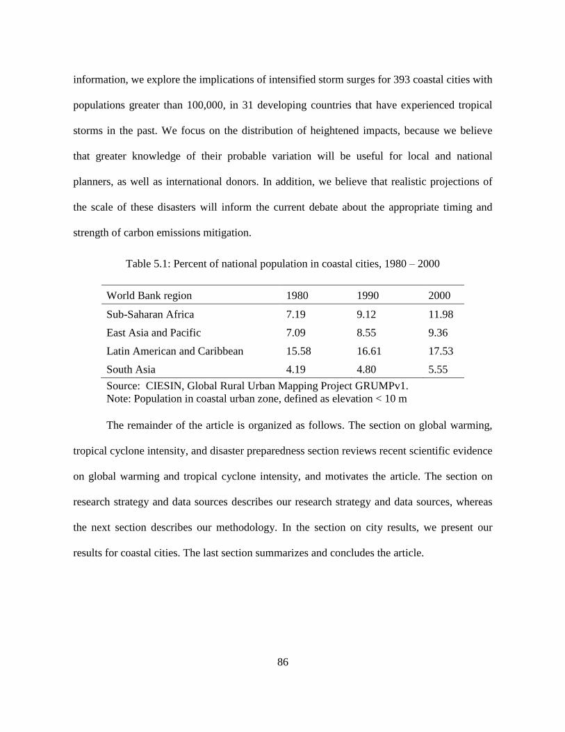
86
information, we explore the implications of intensified storm surges for 393 coastal cities with
populations greater than 100,000, in 31 developing countries that have experienced tropical
storms in the past. We focus on the distribution of heightened impacts, because we believe
that greater knowledge of their probable variation will be useful for local and national
planners, as well as international donors. In addition, we believe that realistic projections of
the scale of these disasters will inform the current debate about the appropriate timing and
strength of carbon emissions mitigation.
Table 5.1: Percent of national population in coastal cities, 1980 – 2000
Source: CIESIN, Global Rural Urban Mapping Project GRUMPv1.
Note: Population in coastal urban zone, defined as elevation < 10 m
The remainder of the article is organized as follows. The section on global warming,
tropical cyclone intensity, and disaster preparedness section reviews recent scientific evidence
on global warming and tropical cyclone intensity, and motivates the article. The section on
research strategy and data sources describes our research strategy and data sources, whereas
the next section describes our methodology. In the section on city results, we present our
results for coastal cities. The last section summarizes and concludes the article.
World Bank region 1980 1990 2000
Sub-Saharan Africa 7.19 9.12 11.98
East Asia and Pacific 7.09 8.55 9.36
Latin American and Caribbean 15.58 16.61 17.53
South Asia 4.19 4.80 5.55
87
5.2 Global Warming, Tropical Cyclone Intensity, and Disaster Preparedness
Some recent scientific studies suggest that observed increases in the frequency and
intensity of tropical cyclones in the last 35 years can be attributed in part to global climate
change (Bengtsson, Hodges, & Roeckner, 2006; Emanuel, 2005; Webster et al., 2005). Others
have challenged this conclusion, citing problems with data reliability, regional variability, and
appropriate measurement of sea surface temperature and other climate variables (e.g.,
Landsea, Harper, Hoarau, & Knaff, 2006). Although the science is not yet conclusive
(International Workshop on Tropical Cyclones, 2006; Pielke, Landsea, Mayfield, Laver, &
Pasch, 2005), the World Meteorological Organization (2006) has recently noted that “it is
likely that some increase in tropical cyclone peak wind-speed and rainfall will occur if the
climate continues to warm. Model studies and theory project a 3-5% increase in wind speed
per degree celsius increase of tropical sea surface temperatures” and “if the projected rise in
sea level due to global warming occurs, then the vulnerability to tropical cyclone storm surge
flooding would increase.”
IPCC (2007, 2011) cite a trend since the mid-1970s toward longer duration and greater
intensity of storms and a strong correlation with the upward trend in tropical sea surface
temperatures. In addition, IPCC (2007) notes that hurricanes/cyclones occur in places where
they have never been observed before. Overall, using a range of model projections, the report
asserts a probability greater than 66% that continued sea surface warming will lead to tropical
cyclones that are more intense, with higher peak wind speeds and heavier precipitation (IPCC,
2007; Emanuel, Sundararajan, & William, 2008; see also Hansen & Sato, 2011; Woodworth
& Blackman, 2004; Woth, Weisse, & von Storch, 2006).
88
These projections from the global scientific community point to the need for greater
disaster preparedness in countries that are vulnerable to storm surges. Some adaptation has
already occurred, and many lives have been saved by improvements in disaster forecasting,
evacuation, and emergency shelter procedures (Shultz, Russell, & Espinel, 2005; Keim,
2006). At the same time, as the recent disasters in Bangladesh and Myanmar have
demonstrated, storm-surge losses remain huge in many areas. Such losses could be reduced by
allocating more resources to increased disaster preparedness, especially given the likelihood
that storms and storm surges will intensify. However, setting a new course requires a better
understanding of expected changes in storm-surge patterns.
5.3 Research Strategy and Data Sources
Previous research on storm-surge impacts on coastal cities has been confined to
relatively limited cases. For example, Hanson et al. (2011) assessed the exposure associated
with surge-induced flood events in 136 port cities with populations of more than one million
in 2005. The impacts of storm surges have been assessed for Bangladesh (Dasgupta et al.,
2010), Copenhagen (Hallegatte et al., 2011), Southern Australia (McInnes, Hubbert,
Macadam, & O’Grady, 2008), the Irish Sea (Wang et al., 2008), and Shanghai (Wang, Gao,
Xu, & Yu, 2010). In this article, we broaden the assessment to 393 coastal cities with
populations greater than 100,000, located in 31 coastal countries that have experienced
tropical storms. These cities are located in four developing regions: East Asia and Pacific,
Latin America and Caribbean, South Asia, and Sub-Saharan Africa. We consider the potential
exposure of these cities to a storm surge that is large (1 in 100 years) by contemporary
standards, and then compare it with a more intense storm surge later in the century. In
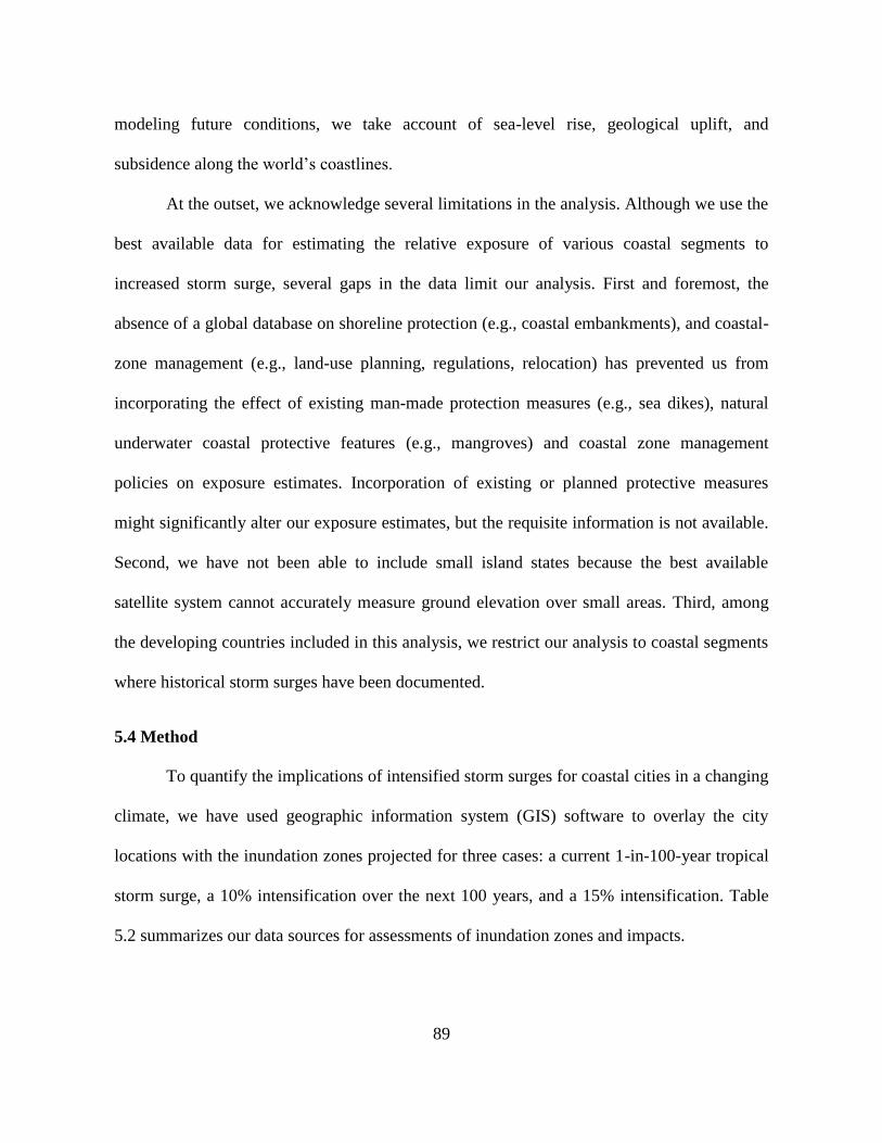
89
modeling future conditions, we take account of sea-level rise, geological uplift, and
subsidence along the world’s coastlines.
At the outset, we acknowledge several limitations in the analysis. Although we use the
best available data for estimating the relative exposure of various coastal segments to
increased storm surge, several gaps in the data limit our analysis. First and foremost, the
absence of a global database on shoreline protection (e.g., coastal embankments), and coastal-
zone management (e.g., land-use planning, regulations, relocation) has prevented us from
incorporating the effect of existing man-made protection measures (e.g., sea dikes), natural
underwater coastal protective features (e.g., mangroves) and coastal zone management
policies on exposure estimates. Incorporation of existing or planned protective measures
might significantly alter our exposure estimates, but the requisite information is not available.
Second, we have not been able to include small island states because the best available
satellite system cannot accurately measure ground elevation over small areas. Third, among
the developing countries included in this analysis, we restrict our analysis to coastal segments
where historical storm surges have been documented.
5.4 Method
To quantify the implications of intensified storm surges for coastal cities in a changing
climate, we have used geographic information system (GIS) software to overlay the city
locations with the inundation zones projected for three cases: a current 1-in-100-year tropical
storm surge, a 10% intensification over the next 100 years, and a 15% intensification. Table
5.2 summarizes our data sources for assessments of inundation zones and impacts.
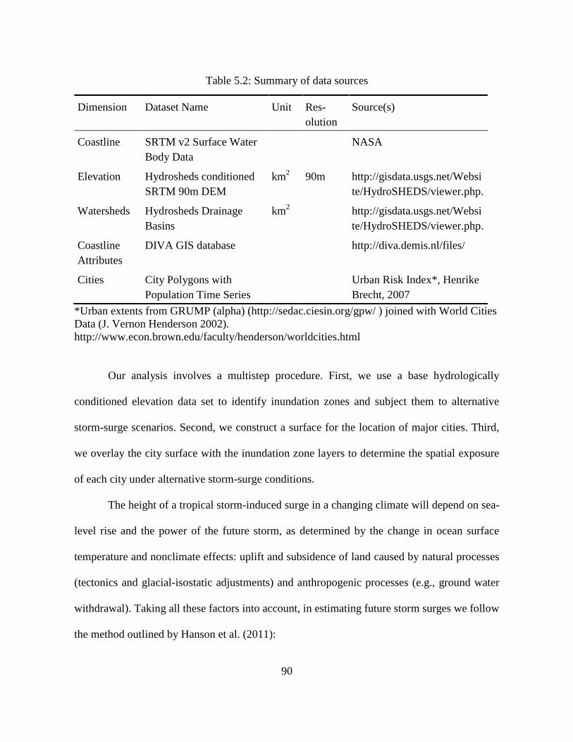
90
Table 5.2: Summary of data sources
Dimension Dataset Name Unit Res-
olution
Source(s)
Coastline SRTM v2 Surface Water
Body Data
NASA
Elevation Hydrosheds conditioned
SRTM 90m DEM
km2 90m http://gisdata.usgs.net/Websi
te/HydroSHEDS/viewer.php.
Watersheds Hydrosheds Drainage
Basins
km2 http://gisdata.usgs.net/Websi
te/HydroSHEDS/viewer.php.
Coastline
Attributes
DIVA GIS database http://diva.demis.nl/files/
Cities City Polygons with
Population Time Series
Urban Risk Index*, Henrike
Brecht, 2007
*Urban extents from GRUMP (alpha) (http://sedac.ciesin.org/gpw/ ) joined with World Cities
Data (J. Vernon Henderson 2002).
http://www.econ.brown.edu/faculty/henderson/worldcities.html
Our analysis involves a multistep procedure. First, we use a base hydrologically
conditioned elevation data set to identify inundation zones and subject them to alternative
storm-surge scenarios. Second, we construct a surface for the location of major cities. Third,
we overlay the city surface with the inundation zone layers to determine the spatial exposure
of each city under alternative storm-surge conditions.
The height of a tropical storm-induced surge in a changing climate will depend on sea-
level rise and the power of the future storm, as determined by the change in ocean surface
temperature and nonclimate effects: uplift and subsidence of land caused by natural processes
(tectonics and glacial-isostatic adjustments) and anthropogenic processes (e.g., ground water
withdrawal). Taking all these factors into account, in estimating future storm surges we follow
the method outlined by Hanson et al. (2011):

91
Future storm surge = S100 + SLR + (UPLIFT × 100 year) / 1000 + SUB + S100 × x
where, S100 = 1-in-100-year current storm surge height (m), SLR = sea-level rise (m),
UPLIFT = continental uplift/ natural subsidence (mm/year), SUB = anthropogenic subsidence
(m) applies to deltas only, x = increase in storm-surge height (%), applied only in coastal
areas that have been affected by cyclones/hurricanes.
More detailed descriptions of the steps followed are provided below:
For elevation, we use a recently released hydrologically conditioned version of 90 m
Shuttle Radan Topography Mission (SRTM) data, part of the hydrosheds data set (Lehner,
Verdin, & Jarvis, 2008). We have downloaded all 5°× 5° coastal tiles of the 90 m SRTM
data, and conditioning of the SRTM data in this case involves steps that alter elevation
values to produce a surface that drains to the coast, including filtering, lowering of stream
courses and adjacent pixels, and carving out barriers to stream flow.
We extract vector coastline masks from SRTM Version 2, and download coastline
information from the Dynamic Interactive Vulnerability Assessment (DIVA) coastal GIS
database. In the calculation of storm surges in a changing 2100 climate, we use the
following attributes drawn from the DIVA database:
S100: 1-in-100-year surge height, based on tidal levels, barometric pressures, wind
speeds, seabed slopes and storm-surge levels from monitoring stations;
DELTAID: coastline segments associated with river deltas;
UPLIFT: estimates of continental uplift/subsidence in mm/year from the geophysical
model of Peltier (2000), including a measure of natural subsidence (2 mm/year) for
deltas.

92
In addition, to approximate conditions in 2100, we assume a SLR of 1 m, 0.5 m
anthropogenic subsidence (SUB) applicable to deltas only, and x = (0.1, 0.15): alternative
increases of 10% and 15% in storm-surge height in coastal areas where tropical cyclones have
occurred.
We compare surges associated with current and future storms with the elevation
values of inland pixels with respect to a coastline, to delineate potential inundation areas.
Each inland pixel could be associated with the nearest coastline segment in a straight-
line distance. However, to better capture the movement of water inland, we use hydrological
drainage basins. We apply the surge height calculated for the coastline segment closest to the
basin outlet to inland areas within that basin.
As a surge moves inland, its height is diminished. The rate of decay depends largely
on terrain and surface features, as well as factors specific to the storm generating the wave. In
a case study on storm surges, Nicholls (2006) uses a distance decay factor of 0.2 to 0.4 m per
kilometer that can be applied to wave heights in relatively flat coastal plains. For this analysis,
we use an intermediate value (0.3 m per 1 km distance from the coastline) to estimate the
wave height for each inland cell.
We delineate surge zones by comparing projected surge heights with SRTM values in
each cell. A cell is part of the surge zone if its elevation value is less than the projected wave.
Following McGranahan, Balk, & Anderson (2007), we delineate low elevation coastal
zones using inland pixels with less than 10 m elevation near coastlines.
For identifying major coastal cities, we have considered all urban agglomerations
containing suburbs and adjacent towns with more than 100,000 inhabitants in the year 2000

93
from the World Cities database. The city points were then matched with the Center for
International Earth Science Information Network (CIESIN) information on global urban
extent based largely on NOAA’s night-time satellite data from 1994 to 1995. For each city a
corresponding raster urban area was identified and converted into a polygon. Where multiple
city points fell within a large contiguous area, Thiessen polygons were used to allocate a
portion of the area to each point, creating a unique urban footprint for each city.
Calculating exposure indicators: We overlay our delineated inundation zones with
locations of cities with more than 100,000 inhabitants in 2000 to determine exposure of 393
coastal cities to storm-surge conditions under current and future climate scenarios.
It should be noted that our estimates may be conservative because (a) the analysis is
based on a sea-level rise estimate of 1 m by 2100, although the previously cited scientific
literature suggests that multi-meter sea-level rise is possible in this century and (b) the
estimates do not take future shoreline erosion into account. As we noted previously, the
absence of a global database on shoreline protection has prevented us from modeling likely
changes in shorelines associated with a 1 m sea-level rise. Even a 1 m rise in sea level will
change shorelines considerably in many coastal segments, if shorelines are not protected
(Dasgupta, Laplante, Murray, & Wheeler, 2011). Coastal morphology will change with
receding shorelines, and potential inundation areas for storm surges will be determined by the
characteristics of the changed coastlines. To improve coastal security, future research and
adaptation planning should consider such likely shoreline changes.
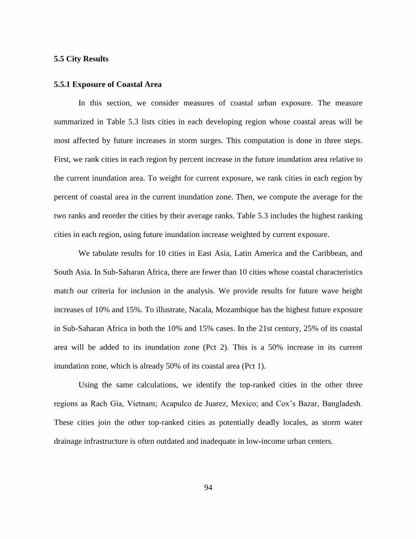
94
5.5 City Results
5.5.1 Exposure of Coastal Area
In this section, we consider measures of coastal urban exposure. The measure
summarized in Table 5.3 lists cities in each developing region whose coastal areas will be
most affected by future increases in storm surges. This computation is done in three steps.
First, we rank cities in each region by percent increase in the future inundation area relative to
the current inundation area. To weight for current exposure, we rank cities in each region by
percent of coastal area in the current inundation zone. Then, we compute the average for the
two ranks and reorder the cities by their average ranks. Table 5.3 includes the highest ranking
cities in each region, using future inundation increase weighted by current exposure.
We tabulate results for 10 cities in East Asia, Latin America and the Caribbean, and
South Asia. In Sub-Saharan Africa, there are fewer than 10 cities whose coastal characteristics
match our criteria for inclusion in the analysis. We provide results for future wave height
increases of 10% and 15%. To illustrate, Nacala, Mozambique has the highest future exposure
in Sub-Saharan Africa in both the 10% and 15% cases. In the 21st century, 25% of its coastal
area will be added to its inundation zone (Pct 2). This is a 50% increase in its current
inundation zone, which is already 50% of its coastal area (Pct 1).
Using the same calculations, we identify the top-ranked cities in the other three
regions as Rach Gia, Vietnam; Acapulco de Juarez, Mexico; and Cox’s Bazar, Bangladesh.
These cities join the other top-ranked cities as potentially deadly locales, as storm water
drainage infrastructure is often outdated and inadequate in low-income urban centers.
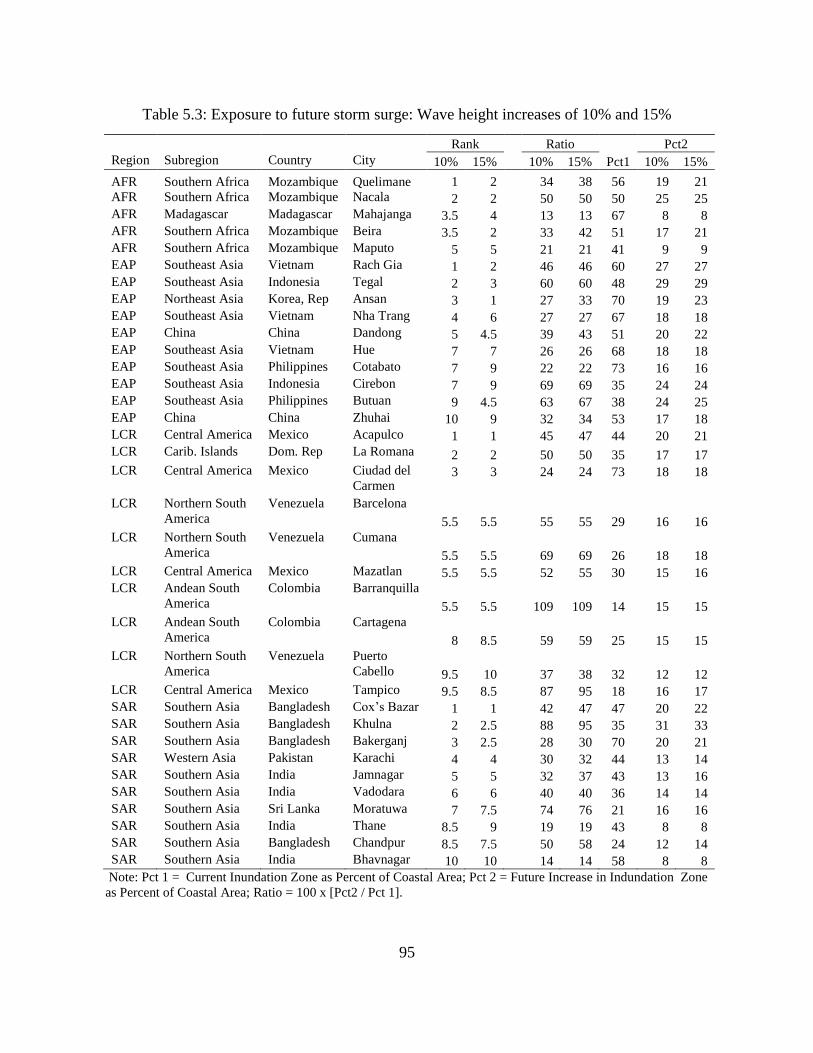
95
Table 5.3: Exposure to future storm surge: Wave height increases of 10% and 15%
Rank
Ratio
Pct2
Region Subregion Country City 10% 15%
10% 15% Pct1 10% 15%
AFR Southern Africa Mozambique Quelimane 1 2 34 38 56 19 21
AFR Southern Africa Mozambique Nacala 2 2 50 50 50 25 25
AFR Madagascar Madagascar Mahajanga 3.5 4 13 13 67 8 8
AFR Southern Africa Mozambique Beira 3.5 2 33 42 51 17 21
AFR Southern Africa Mozambique Maputo 5 5 21 21 41 9 9
EAP Southeast Asia Vietnam Rach Gia 1 2 46 46 60 27 27
EAP Southeast Asia Indonesia Tegal 2 3 60 60 48 29 29
EAP Northeast Asia Korea, Rep Ansan 3 1 27 33 70 19 23
EAP Southeast Asia Vietnam Nha Trang 4 6 27 27 67 18 18
EAP China China Dandong 5 4.5 39 43 51 20 22
EAP Southeast Asia Vietnam Hue 7 7 26 26 68 18 18
EAP Southeast Asia Philippines Cotabato 7 9 22 22 73 16 16
EAP Southeast Asia Indonesia Cirebon 7 9 69 69 35 24 24
EAP Southeast Asia Philippines Butuan 9 4.5 63 67 38 24 25
EAP China China Zhuhai 10 9 32 34 53 17 18
LCR Central America Mexico Acapulco 1 1 45 47 44 20 21
LCR Carib. Islands Dom. Rep La Romana 2 2 50 50 35 17 17
LCR Central America Mexico Ciudad del
Carmen 3 3 24 24 73 18 18
LCR Northern South
America
Venezuela Barcelona
5.5 5.5 55 55 29 16 16
LCR Northern South
America
Venezuela Cumana
5.5 5.5 69 69 26 18 18
LCR Central America Mexico Mazatlan 5.5 5.5 52 55 30 15 16
LCR Andean South
America
Colombia Barranquilla
5.5 5.5 109 109 14 15 15
LCR Andean South
America
Colombia Cartagena
8 8.5 59 59 25 15 15
LCR Northern South
America
Venezuela Puerto
Cabello 9.5 10 37 38 32 12 12
LCR Central America Mexico Tampico 9.5 8.5 87 95 18 16 17
SAR Southern Asia Bangladesh Cox’s Bazar 1 1 42 47 47 20 22
SAR Southern Asia Bangladesh Khulna 2 2.5 88 95 35 31 33
SAR Southern Asia Bangladesh Bakerganj 3 2.5 28 30 70 20 21
SAR Western Asia Pakistan Karachi 4 4 30 32 44 13 14
SAR Southern Asia India Jamnagar 5 5 32 37 43 13 16
SAR Southern Asia India Vadodara 6 6 40 40 36 14 14
SAR Southern Asia Sri Lanka Moratuwa 7 7.5 74 76 21 16 16
SAR Southern Asia India Thane 8.5 9 19 19 43 8 8
SAR Southern Asia Bangladesh Chandpur 8.5 7.5 50 58 24 12 14
SAR Southern Asia India Bhavnagar 10 10 14 14 58 8 8
Note: Pct 1 = Current Inundation Zone as Percent of Coastal Area; Pct 2 = Future Increase in Indundation Zone
as Percent of Coastal Area; Ratio = 100 x [Pct2 / Pct 1].
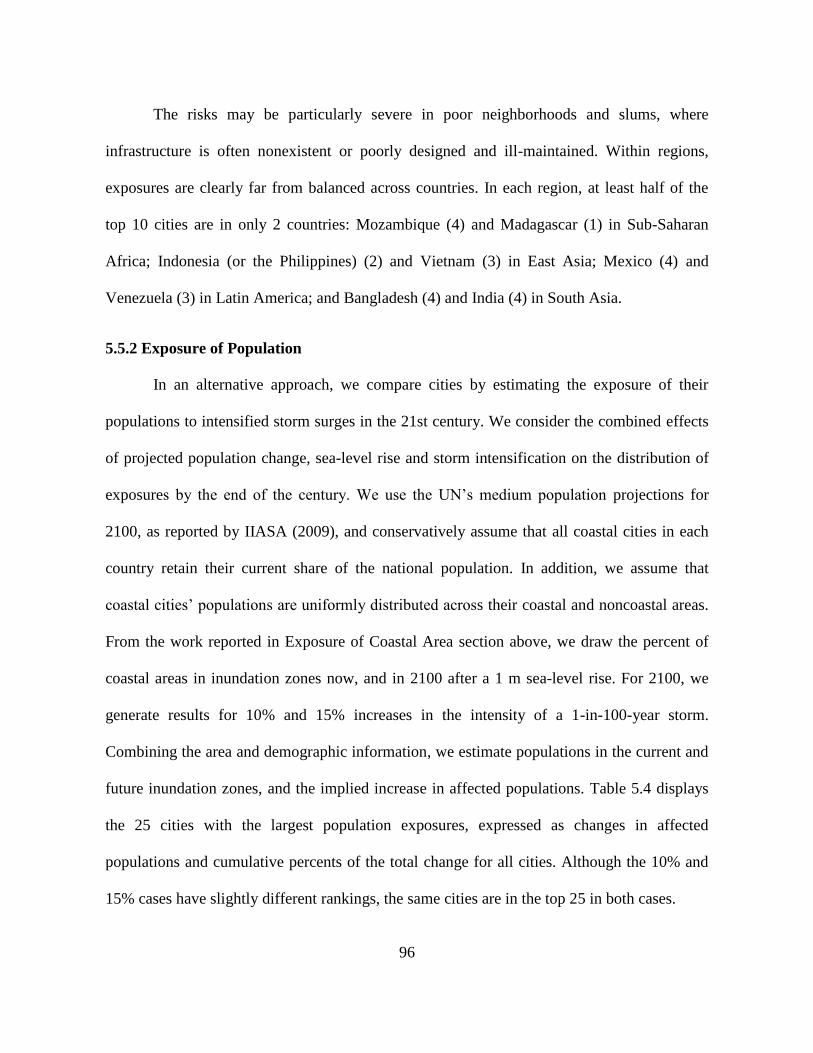
96
The risks may be particularly severe in poor neighborhoods and slums, where
infrastructure is often nonexistent or poorly designed and ill-maintained. Within regions,
exposures are clearly far from balanced across countries. In each region, at least half of the
top 10 cities are in only 2 countries: Mozambique (4) and Madagascar (1) in Sub-Saharan
Africa; Indonesia (or the Philippines) (2) and Vietnam (3) in East Asia; Mexico (4) and
Venezuela (3) in Latin America; and Bangladesh (4) and India (4) in South Asia.
5.5.2 Exposure of Population
In an alternative approach, we compare cities by estimating the exposure of their
populations to intensified storm surges in the 21st century. We consider the combined effects
of projected population change, sea-level rise and storm intensification on the distribution of
exposures by the end of the century. We use the UN’s medium population projections for
2100, as reported by IIASA (2009), and conservatively assume that all coastal cities in each
country retain their current share of the national population. In addition, we assume that
coastal cities’ populations are uniformly distributed across their coastal and noncoastal areas.
From the work reported in Exposure of Coastal Area section above, we draw the percent of
coastal areas in inundation zones now, and in 2100 after a 1 m sea-level rise. For 2100, we
generate results for 10% and 15% increases in the intensity of a 1-in-100-year storm.
Combining the area and demographic information, we estimate populations in the current and
future inundation zones, and the implied increase in affected populations. Table 5.4 displays
the 25 cities with the largest population exposures, expressed as changes in affected
populations and cumulative percents of the total change for all cities. Although the 10% and
15% cases have slightly different rankings, the same cities are in the top 25 in both cases.
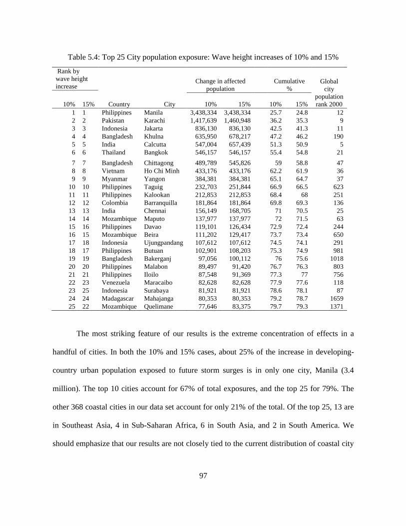
97
Table 5.4: Top 25 City population exposure: Wave height increases of 10% and 15%
Rank by
wave height
increase
Change in affected
population
Cumulative
% Global
city
population
rank 2000
10% 15% Country City 10% 15% 10% 15%
1 1 Philippines Manila 3,438,334 3,438,334 25.7 24.8 12
2 2 Pakistan Karachi 1,417,639 1,460,948 36.2 35.3 9
3 3 Indonesia Jakarta 836,130 836,130 42.5 41.3 11
4 4 Bangladesh Khulna 635,950 678,217 47.2 46.2 190
5 5 India Calcutta 547,004 657,439 51.3 50.9 5
6 6 Thailand Bangkok 546,157 546,157 55.4 54.8 21
7 7 Bangladesh Chittagong 489,789 545,826 59 58.8 47
8 8 Vietnam Ho Chi Minh 433,176 433,176 62.2 61.9 36
9 9 Myanmar Yangon 384,381 384,381 65.1 64.7 37
10 10 Philippines Taguig 232,703 251,844 66.9 66.5 623
11 11 Philippines Kalookan 212,853 212,853 68.4 68 251
12 12 Colombia Barranquilla 181,864 181,864 69.8 69.3 136
13 13 India Chennai 156,149 168,705 71 70.5 25
14 14 Mozambique Maputo 137,977 137,977 72 71.5 63
15 16 Philippines Davao 119,101 126,434 72.9 72.4 244
16 15 Mozambique Beira 111,202 129,417 73.7 73.4 650
17 18 Indonesia Ujungpandang 107,612 107,612 74.5 74.1 291
18 17 Philippines Butuan 102,901 108,203 75.3 74.9 981
19 19 Bangladesh Bakerganj 97,056 100,112 76 75.6 1018
20 20 Philippines Malabon 89,497 91,420 76.7 76.3 803
21 21 Philippines Iloilo 87,548 91,369 77.3 77 756
22 23 Venezuela Maracaibo 82,628 82,628 77.9 77.6 118
23 25 Indonesia Surabaya 81,921 81,921 78.6 78.1 87
24 24 Madagascar Mahajanga 80,353 80,353 79.2 78.7 1659
25 22 Mozambique Quelimane 77,646 83,375 79.7 79.3 1371
The most striking feature of our results is the extreme concentration of effects in a
handful of cities. In both the 10% and 15% cases, about 25% of the increase in developing-
country urban population exposed to future storm surges is in only one city, Manila (3.4
million). The top 10 cities account for 67% of total exposures, and the top 25 for 79%. The
other 368 coastal cities in our data set account for only 21% of the total. Of the top 25, 13 are
in Southeast Asia, 4 in Sub-Saharan Africa, 6 in South Asia, and 2 in South America. We
should emphasize that our results are not closely tied to the current distribution of coastal city
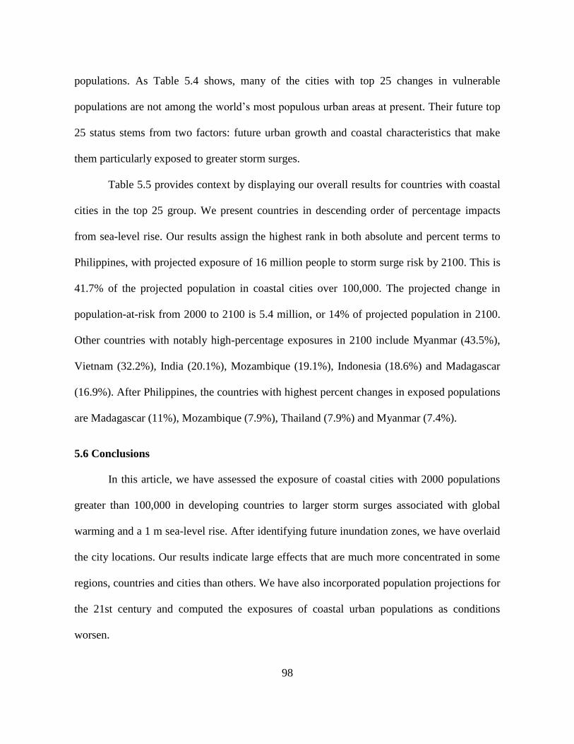
98
populations. As Table 5.4 shows, many of the cities with top 25 changes in vulnerable
populations are not among the world’s most populous urban areas at present. Their future top
25 status stems from two factors: future urban growth and coastal characteristics that make
them particularly exposed to greater storm surges.
Table 5.5 provides context by displaying our overall results for countries with coastal
cities in the top 25 group. We present countries in descending order of percentage impacts
from sea-level rise. Our results assign the highest rank in both absolute and percent terms to
Philippines, with projected exposure of 16 million people to storm surge risk by 2100. This is
41.7% of the projected population in coastal cities over 100,000. The projected change in
population-at-risk from 2000 to 2100 is 5.4 million, or 14% of projected population in 2100.
Other countries with notably high-percentage exposures in 2100 include Myanmar (43.5%),
Vietnam (32.2%), India (20.1%), Mozambique (19.1%), Indonesia (18.6%) and Madagascar
(16.9%). After Philippines, the countries with highest percent changes in exposed populations
are Madagascar (11%), Mozambique (7.9%), Thailand (7.9%) and Myanmar (7.4%).
5.6 Conclusions
In this article, we have assessed the exposure of coastal cities with 2000 populations
greater than 100,000 in developing countries to larger storm surges associated with global
warming and a 1 m sea-level rise. After identifying future inundation zones, we have overlaid
the city locations. Our results indicate large effects that are much more concentrated in some
regions, countries and cities than others. We have also incorporated population projections for
the 21st century and computed the exposures of coastal urban populations as conditions
worsen.
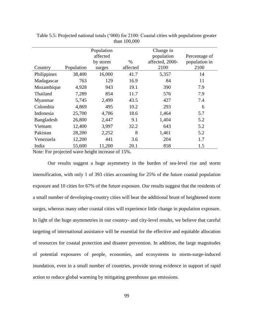
99
Table 5.5: Projected national totals (‘000) for 2100: Coastal cities with populations greater
than 100,000
Country Population
Population
affected
by storm
surges
%
affected
Change in
population
affected, 2000-
2100
Percentage of
population in
2100
Philippines 38,400 16,000 41.7 5,357 14
Madagascar 763 129 16.9 84 11
Mozambique 4,928 943 19.1 390 7.9
Thailand 7,289 854 11.7 576 7.9
Myanmar 5,745 2,499 43.5 427 7.4
Colombia 4,869 495 10.2 293 6
Indonesia 25,700 4,786 18.6 1,464 5.7
Bangladesh 26,800 2,447 9.1 1,404 5.2
Vietnam 12,400 3,997 32.2 643 5.2
Pakistan 28,200 2,252 8 1,461 5.2
Venezuela 12,200 441 3.6 204 1.7
India 55,600 11,200 20.1 858 1.5
Note: For projected wave height increase of 15%.
Our results suggest a huge asymmetry in the burden of sea-level rise and storm
intensification, with only 1 of 393 cities accounting for 25% of the future coastal population
exposure and 10 cities for 67% of the future exposure. Our results suggest that the residents of
a small number of developing-country cities will bear the additional brunt of heightened storm
surges, whereas many other coastal cities will experience little change in population exposure.
In light of the huge asymmetries in our country- and city-level results, we believe that careful
targeting of international assistance will be essential for the effective and equitable allocation
of resources for coastal protection and disaster prevention. In addition, the large magnitudes
of potential exposures of people, economies, and ecosystems to storm-surge-induced
inundation, even in a small number of countries, provide strong evidence in support of rapid
action to reduce global warming by mitigating greenhouse gas emissions.
100
5.7 References
Bangladesh Disaster Management Information Centre (2007). Cyclonic storm “SIDR.”
[Retrieved from http://www.reliefweb.int/rw/RWFiles2007.nsf/FilesByRWDocUnid
Filename/EDIS-79BQ9Z-full_report.pdf/$File/full_report.pdf].
Bengtsson, L., K. I. Hodges & E. Roeckner (2006). Storm tracks and climate change. Journal
of Climate, 19: 3518-3543.
Brecht, H. (2007). A Global Urban Risk Index: Analyzing mortality and economic threats
from natural hazards. Washington, DC: World Bank.
Centre for International Earth Science Information Network (CIESIN), Columbia University;
International Food Policy Research Institute (IPFRI); The World Bank; Centro
Internacional de Agricultura Tropical (CIAT) (2005). Global Rural Urban Mapping
Project (GRUMP), Alpha Version. Palisades, NY: Socioeconomic Data and
Applications Center (SEDAC), Columbia University. [Retrieved from
http://sedac.ciesin.columbia.edu/gpw/].
Dasgupta, S., M. Huq, Z. H. Khan, M. M. Z. Ahmed, N. Mukherjee, M. F. Khan & K. Pandey
(2010). Vulnerability of Bangladesh to cyclones in a changing climate: Potential
damages and adaptation cost. Policy Research Working Paper No. 5280.
Washington, DC: World Bank.
Dasgupta, S., B. Laplante, S. Murray, D. Wheeler (2011). Exposure of developing countries
to sea-level rise and storm surges. Climatic Change, 106: 567-579.
Dasgupta, S. & C. Meisner (2009). Climate change and sea-level rise: A review of the
scientific evidence. Environment Department Paper No. 118. Washington, DC: World
Bank.
Emanuel, K. (2005). Increasing destructiveness of tropical cyclones over the past 30 years.
Nature, 436: 686-688.
Emanuel, K., R. Sundararajan & J. William (2008). Hurricanes and global warming: Results
from downscaling IPCC AR4 simulations. Journal of Climate, 89: 347-367.
Ericson, J. P., C. J. Vörösmarty, S. L. Dingman, L.G.Ward & M. Meybeck (2006).
Effective sea-level rise and deltas: Causes of change and human dimension
implications. Global and Planetary Change, 50: 63-82.
101
Gorokhovich, Y. & A. Voustianiouk. (2006). Accuracy assessment of the processed
SRTMbased elevation data by CGIAR using field data from USA and Thailand and its
relation to the terrain characteristics. Remote Sensing of Environment, 104: 409-415.
Hallegatte, S., N. Ranger, O. Mestre, P. Dumas, J. Corfee-Morlot, C. Herweijer & R. M.
Wood (2011). Assessing climate change impacts, sea-level rise, and storm surge risk
in Port cities: A case study on Copenhagen. Climatic Change, 104: 113-137.
Hansen, J. (2006). Can we still avoid dangerous human-made climate change? Presentation to
the American Geophysical Union in San Francisco, CA. [Retrieved from
http://www.columbia.edu/~jeh1/newschool_text_and_slides.pdf].
Hansen, J. (2007). Scientific reticence and sea-level rise. Environmental Research Letters.
Advance online publication. DOI:10.1088/1748-9326/2/2/024002.
Hanson, S., R. Nicholls, N. Ranger, S. Hallegatte, J. Corfee-Morlot, C. Herweijer & J.
Chateau (2011). A global ranking of port cities with high exposure to climate
extremes. Climatic Change, 104: 89-111.
Hansen, J. E. & M. Sato (2011). Paleoclimate implications for human-made climate change.
[Retrieved from http://www.columbia.edu/~jeh1/mailings/2011/20110118
_Milankovic-Paper.pdf].
Hardy, T., Mason, L., & Astorquia, A. (2004). The frequency of surge plus tide during
tropical cyclones for selected open coast locations along the Queensland East Coast,
Queensland climate change and community vulnerability to tropical cyclones: Ocean
hazards assessment: Stage 3 report. [Retrieved from http://www.iiasa.ac.at/
webapps/ggi/GgiDb/dsd?Action=htmlpage&page=countries].
Intergovernmental Panel on Climate Change (IPCC) (2007). Climate change 2007: The
physical science basis, summary for policymakers. Geneva, Switzerland: IPCC.
Intergovernmental Panel on Climate Change (IPCC) (2011). Summary for policymakers. In
Intergovernmental Panel on Climate Change: Special report on managing the
risks of extreme events and disasters to advance climate change adaptation, eds. C. B.
Field, V. Barros, T. F. Stocker, D. Qin, D. Dokken, K. L. Ebi, P. M. Midgley.
Cambridge, UK: Cambridge University Press. [Retrieved from http://ipcc-
wg2.gov/SREX/].
International Workshop on Tropical Cyclones (2006). Statement on tropical cyclones and
climate change. [Retrieved from http://www.gfdl.noaa.gov/~tk/glob_warm_
hurr.html].
102
Karim, M. K. & N. Mimura (2008). Impacts of climate change and sea-level rise on
cyclonic storm surge floods in Bangladesh. Global Environmental Change, 18: 490-
500.
Keim, M. E. (2006). Cyclones, tsunamis, and human health. Oceanography, 19(2): 40-49.
Knutson, T. R. & R. E. Tuleya (2004). Impact of CO2-induced warming on simulated
hurricane intensity and precipitation sensitivity to the choice of climate model and
convective parameterization. Journal of Climate, 17: 3477-3495.
Knutson, T. R., J. L. McBride, J. Chan, K. Emanuel, G. Holland, C. Landsea & M. Sugi,
(2010). Tropical cyclones and climate change. Nature Geoscience, 3: 157-163.
Landsea, C. W., B. A. Harper, K. Hoarau & J.A. Knaff (2006). Climate change: Can we
detect trends in extreme tropical cyclones? Science, 313: 452-454.
Lehner, B. & P. Döll (2004). Development and validation of a global database of lakes,
reservoirs and wetlands. Journal of Hydrology, 296(1-4): 1-22.
Lehner, B., K. Verdin, & A. Jarvis (2008). New global hydrography derived from spaceborne
elevation data. EOS, Transactions, AGU, 89: 93-94.
Mazzotti, S., A. Lambert, M. Van der Kooij & A. Mainville (2009). Impact of
anthropogenic subsidence on relative sea-level rise in the Fraser River delta. Geology,
37: 771-774.
McGranahan, G., D. Balk & B. Anderson (2007). The rising tide: Assessing the risks of
climate change and human settlements in low elevation coastal zones. Environment &
Urbanization, 19(1): 17-37.
McInnes, K. L., G. D. Hubbert, I. Macadam & J. G. O’Grady (2008). Assessing the impact
of climate change on storm surges in Southern Australia. [Retrieved from
[http://www.mssanz.org.au/MODSIM07/papers/26_s32/AssessingTheImpact_s32_Mc
Innes_.pdf].
McInnes, K. L., I. Macadam, G. D. Hubbert, D. J. Abbs & J. A. Bathols (2005). Climate
change in Eastern Victoria stage 2 report: The effect of climate change on storm
surges. Aspendale, VIC: CSIRO Marine and Atmospheric Research.
Michaels, P. J., P. C. Knappenberger & R. E. Davis (2005). Sea-surface temperatures and
tropical cyclones: Breaking the Paradigm. Presented at the 15th conference of
Applied Climatology. [Retrieved from http://ams.confex.com/ams/
15AppClimate/techprogram/paper_94127.htm].
103
Nicholls, R. J. (2003). An expert assessment of storm surge “hotspots.” Final Report (Draft
Version) to Center for Hazards and Risk Research, Lamont-Dohert Observatory,
Columbia University, New York, NY.
Nicholls, R. J. (2006). Storm surges in coastal areas. Natural disaster hot spots case studies.
Washington, DC: World Bank.
Nicholls, R. J., S. Brown & S. Hanson (2010). Economics of coastal zone: Adaptation to
climate change. World Bank Environment Department Paper No. 10. [Retrieved from
http:// beta.worldbank.org/sites/default/files/documents/
DCCDP_10_CoastalZoneAdaptation .pdf].
Overpeck, J., B. Otto-Bliesner, G. Miller, D. Muhs, R. Alley & J. Kiehl (2006). Paleoclimatic
evidence for future ice-sheet instability and rapid sea-level rise. Science, 311: 1747-
1750.
Pfeffer, W. T., J. T. Harper & S. O’Neel (2008). Kinematic constraints on glacier
contributions to 21st century sea-level rise. Science, 321: 1340-1343.
Peltier, W. R. (2000). Glacial isostatic adjustment corrections. In Sea level rise: History and
consequences, eds. B. C. Douglas, M. S. Kearney & S. P. Letherman, 65-93. San
Diego, CA: Academic Press.
Pielke, R. A., C. Landsea, M. Mayfield, J. Laver & R. Pasch (2005). Hurricanes and global
warming. Bulletin of American Meteorological Society, 86: 1571-1575.
Rahmstorf, S. (2007). A semi-empirical approach to projecting future sea-level rise. Science,
315, 368-370.
Shultz, J. M., J. Russell & Z. Espinel (2005). Epidemiology of tropical cyclones: The
dynamics of disaster, disease, and development. Epidemiologic Reviews, 27: 21-35.
Syvitski, J. P. M., A. J. Kettner, I. Overeem, E. W. H. Hutton, M. T. Hannon, G. R.
Brakenridge & R. J. Nicholls (2009). Sinking deltas due to human activities. Nature
Geoscience, 2: 681-686.
United Nations (UN) (2007). SIDR Cyclone Bangladesh 2007 (Emergency report, Sit Rep No.
14.). [Retrieved from http://www.searo.who.int/LinkFiles/Bangladesh_2007-12-
12_UN_Ban14.pdf].
United Nations (UN) (2008). Post-Nargis Joint Assessment. [Retrieved from
http://www.aseansec.org/21765.pdf].
104
United Nations International Strategy for Disaster Reduction Secretariat (ISDR) (2009).
Global assessment report on disaster risk reduction. Geneva: ISDR. [Retrieved from
http://www.preventionweb.net/english/hyogo/gar/report/].
Vafeidis, A. T., R. J. Nicholls, L. McFadden, R. S. J. Tol, J. Hinkel, T. Spencer & R. J. T.
Klein (2008). A new global coastal database for impact and vulnerability analysis to
sea-level rise. Journal of Coastal Research, 24: 917-924.
Vermeer, M. & S. Rahmstorf (2009). Global sea level linked to global temperature.
Proceedings of the National Academy of Sciences, 106: 21527-21532.
Wang, J., W. Gao, S. Xu & L. Yu (2010). Evaluation of the combined risk of sea level rise,
land subsidence, and storm surges, and strategies for minimizing damage to coastal
areas of Shanghai, China. Climatic Change: DOI: 10.1007/s10584-012-0468-7.
Wang, S., R. McGrath, J. Hanafin, P. Lynch, T. Semmler & P. Nolan (2008). The impact of
climate change on storm surges over Irish waters. Ocean Modeling, 25(1-2): 83-94.
Webster, P. J., G. J. Holland, J. A. Curry & H.-R. Chang (2005). Changes in tropical
cyclone number, duration, and intensity in a warming environment. Science, 309:
1844-1846.
Woodworth, P. L. & D. L. Blackman (2004). Evidence for systematic changes in extreme
high waters since the mid-1970s. Journal of Climate, 17: 1190-1197.
World Meteorological Organization (WMO) (2006). Sixth international workshop on tropical
cyclones of the World Meteorological Organization. San José, Costa Rica: WMO.
Woth, K., R. Weisse & H. von Storch (2006). Climate change and North Sea storm surge
extremes: An ensemble study of storm surge extremes expected in a changed climate
projected by four different regional climate models. Ocean Dynamics, 56(1): 3-15.
105
CHAPTER 6 : CONCLUSION
CONCLUSION
6.1 Summary and Main Conclusions
The primary goal of this study was to contribute to a reversal of the staggering disaster
losses by advancing the application of GIS in the field of disaster risk management.
In Chapter 2, I set the stage for this dissertation by introducing its topic using the
example of Louisiana and its vulnerability to hurricanes. The formation and anatomy of
hurricanes along with their frequency near the Louisiana coast were described. The chapter
outlined the importance but also the unprecedented loss of the Louisiana wetlands and
discusses coastal restoration efforts as a means to reduce hurricane risks.
With a clearer understanding of the concepts of disasters, vulnerability, and risk
reduction, this dissertation then examined four case studies that implement GIS
methodologies in disaster risk management, specifically in the fields of emergency
preparedness and risk assessments. A set of research questions was posed corresponding to
the two fields above.
Emergency Preparedness
In chapter 3, I focused on the application of GIS in emergency preparedness with the
goal to promote the use of GIS in disaster response and thereby enhance decision making in
the aftermath of catastrophes. The research question was:
1. How can the application of GIS be improved in the emergency response phase?
106
Chapter 3 addressed the second research question. Through interviews with GIS
responders in the three U.S. States of Louisiana, Alabama, and Mississippi after Hurricane
Katrina in 2005, the successes and failures of using geographic information to support the
response were investigated and lessons were drawn. The study showed that the use of GIS in
the emergency phase differs from that in the planning phase due to the urgency, uncertainty,
and the fast coordination of a multitude of stakeholders. Truly analytic GIS applications going
beyond simple mapping were sparse. The main challenges in the operations were not related
to the prominent literature themes of Virtual Reality and semantics but rather trivial issues
had to be solved such as missing metadata and the lack of a platform to effectively distribute
the data to emergency responders. The intensive use of web tools, such as Google Earth,
proved to be successful due to their ease of use. Such web tools could be operated by non-GIS
specialists and allowed for straightforward and helpful applications, such as the overlay of
imagery before and after the disaster. One main takeaway is that a GIS contingency plan,
drafted before the disaster, is critical for a successful emergency response. The plan should
address a multitude of issues including the work of volunteers, data readiness through GIS
clearinghouses, and tools for information dissemination.
Risk Assessments
In chapters 4 and 5, attention was directed towards risk assessments as instruments for
determining the likelihood of an extreme hazard event and climate change impacts. The main
research questions were:
1. Which cities are likely to be affected by a disaster?
2. In which cities is the risk of mortality due to a natural hazard the highest?
107
3. Which cities are most at risk of economic losses due to natural hazards?
4. Which cities will be highly impacted by climate change and storm surges?
To seek answers to these questions, I have made use of global data layers for cities,
hazards, vulnerability, exposure, and watersheds and analyzed them in a novel GIS process.
To address the first three questions, I developed a ranking of the major cities in 110 countries.
Risk levels of 1,943 cities with more than 100,000 inhabitants in the year 2000 were evaluated
and compared for the four major hazards of cyclones, earthquakes, floods, and landslides.
Urban risks were identified for each of these hazards separately, and, in addition, a multi-
hazard index gave a holistic picture of city risk. The index showed that risk is highly
concentrated in a number of cities in certain regions. Asia is particular prone to disasters. Out
of the most at risk 30 cities, eleven are in East Asia and five in South Asia. In Latin America,
Mexico City, Sao Paulo, and Buenos Aires have the highest disaster risks. In Sub-Saharan
Africa, cities in South Africa are at high risk, especially to floods.
Chapter 5 contained a discussion of the fourth question as stated above, where,
building upon the results of chapter 4, I considered the strategies that can be employed to
include the impacts of climate change in the urban risk assessment. The implications of storm
surges for coastal cities were quantified both for contemporary conditions and for expected
future conditions in a changing climate. The exposure to today’s and future storm surges were
explored for 393 of cyclone-vulnerable coastal cities in 31 developing countries. To model the
future conditions, sea-level rise, geological uplift, and subsidence of coastlines were taken
into account. The most striking feature of the results was the extreme concentration of effects
in a handful of cities. The analysis suggested gross inequality in the heightened impact of
108
future disasters, with 50% of the burden falling on the residents of ten Asian cities and 40%
falling on Manila, Karachi, and Jakarta alone. In light of these huge asymmetries, careful
targeting of international assistance will be essential for the effective and equitable allocation
of resources for coastal protection and disaster prevention.
This dissertation thus presented several case studies that demonstrated how geospatial
methods can be applied in disaster risk management. There are reasons to believe that the
cooperation between these two fields will continue to expand and deepen which will no doubt
lead to more effective and efficient disaster risk management with direct consequences for a
safer life.
6.2 A Short Glance Ahead
Emergency Preparedness
Further research is necessary to investigate how promising new technologies can be
applied to best save lives and property. For example, Web 2.0, as a technology that provides a
platform for information sharing, interoperability, user interaction, and collaboration on the
World Wide Web, has large potential to enhance disaster preparedness. It allows for viewers
of content to become active contributors and creators in a virtual community. In the last few
years, we have seen an exciting shift in how GIS paired with Web 2.0 technologies can
support disaster risk management programs. An interesting study could document how Web
2.0 tools are being used in emergencies and investigate further applications. Empowered by
cloud-, crowd-, and SMS-based technologies, remote technological communities can now
engage in disaster response at an unprecedented level. Especially the year 2010 marked a
change in how GIS supports humanitarian emergencies: After the 2010 earthquakes in Haiti
109
and Chile and the floods in Pakistan, volunteer communities, often with extensive expertise in
GIS, mobilized and processed imagery, created detailed maps, and geocoded an abundance of
houses, streets, and critical infrastructure. Using open source and cloud-based tools, these
humanitarian technologists applied their skills to help affected communities and reduce risks.
Prominent applications include OpenStreetMap, an open collection of data being gathered by
currently over 300,000 members, Ushahidi, an open-source crowd sourcing crisis information
platform, and GoogleMapMaker, which allows its members to collaboratively create maps.
The outputs support the humanitarian response and help to provide speedy and efficient aid to
the ones most in need. We are only at the beginning of using the full potential of these
technologies, and a study on this development could provide great insights on where to go
from here.
But also public institutions are moving towards fully embracing GIS as a basis for
emergency preparedness. Another worthy research effort could document the best practices in
GIS applications used in emergency centers around the world. During my employment at the
World Bank, I have enjoyed working, for example, in the Emergency Operations
Coordination Centers of Queensland, Australia, and Shanghai, China. Both centers have
anchored their operations fully in GIS and have developed GIS customized applications as the
main platform for the emergency centers with a plethora of baseline data and pre-defined
automated ways to add data in emergencies. Armed with this system, emergency services
personnel can effectively carry out its task, including evacuating communities and
strategically positioning their crews and resources, where they are clear of rising waters or
burning fires.

110
Risk Assessments
This dissertation is only a first step in creating an integrated framework for assessing
urban disaster risk. Much work needs to be done both on local and global levels to complete
the picture. Since the most limiting factor is the lack of accurate and systematic loss data, the
improvement and refinement of the underlying loss databases are essential. Several regional
initiatives are already ongoing to build capacity for assessing damages and losses and
developing regional databases for post-event loss data. For instance, the Association of
Southeast Asian Nations (ASEAN) has included the development of damage and loss
databases into its work program 2010–2015 (ASEAN 2010) and is currently supporting its
member states to set up uniform systems for recording post-event event data. To scale up
these initiatives, the World Bank and the Global Facility for Disaster Reduction and Recovery
have been providing training for Governments in damage and loss assessments for more than
50 countries. Yet, further studies and efforts are needed to complete the picture of historic
losses.
Another restrictive factor to develop accurate urban risk assessments is the
approximations used for the hazard layers. Future versions of the index will be able to make
use of advanced hazard models, such the one being currently developed by the Global
Earthquake Model (GEM) foundation and for the Global Assessment Report 2013, which is
currently being developed by the United Nations International Strategy for Disaster Reduction
(UN-ISDR).
Additional research could also provide greater insights into how to increase the use
and application of risk assessments in development and land use planning. Sharing risk
111
information, such as maps of flood plains and seismic fault lines, widely and in a form that is
readily understood is an easy and effective measure to reduce risk. Open risk information
would, for instance, facilitate holding officials accountable in the case they do not address
known risks. Also, real estate markets could better reflect risk information in housing prices,
which would depreciate house prices in risky areas and lead to incentives to not invest in new
development in hazardous locations. While the importance of sharing data is increasingly
being recognized, there are still many obstacles to achieving open data practices. Future
research can investigate how to best publicize risk information and incentivize its use in
planning. This could include studies on fostering government commitments to open data for
promoting transparency, accountability, and improved decision making and also research on
open source software tools to share, source and create disaster risk data.

112
APPENDIX 1: GLOBAL URBAN RISK INDEX - CITY RANKING
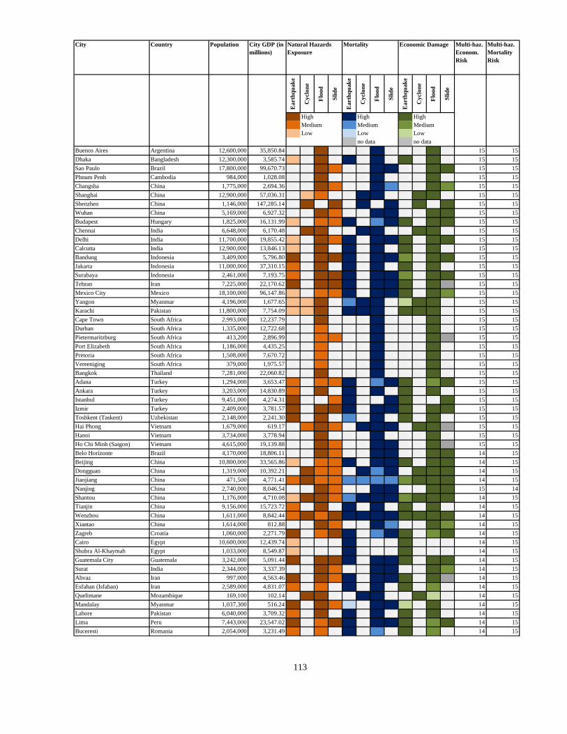
City Country Population City GDP (in
millions)
Multi-haz.
Econom.
Risk
Multi-haz.
Mortality
Risk
Ea
rth
qu
ak
e
Cy
clo
ne
Flo
od
Sli
de
Ea
rth
qu
ak
e
Cy
clo
ne
Flo
od
Sli
de
Ea
rth
qu
ak
e
Cy
clo
ne
Flo
od
Sli
de
3 High 3 High 3 High
2 Medium 2 Medium 2 Medium
1 Low 1 Low 1 Low
no data no data
Buenos Aires Argentina 12,600,000 35,850.84 0 0 3 0 0 0 3 0 0 0 3 0 15 15
Dhaka Bangladesh 12,300,000 3,585.74 1 0 3 0 3 0 3 0 3 0 3 0 15 15
Sao Paulo Brazil 17,800,000 99,670.73 0 0 3 2 0 0 3 3 0 0 3 3 15 15
Phnum Penh Cambodia 984,000 1,028.08 0 0 3 0 0 0 3 0 0 0 3 0 15 15
Changsha China 1,775,000 2,694.36 0 0 3 2 0 0 3 2 0 0 3 2 15 15
Shanghai China 12,900,000 57,036.31 0 1 2 0 0 3 3 0 0 3 3 0 15 15
Shenzhen China 1,146,000 147,285.14 0 3 0 3 0 3 0 3 0 3 0 3 15 15
Wuhan China 5,169,000 6,927.32 0 0 3 2 0 0 3 3 0 0 3 3 15 15
Budapest Hungary 1,825,000 16,131.99 1 0 2 2 3 0 2 3 3 0 3 3 15 15
Chennai India 6,648,000 6,170.48 0 3 3 0 0 3 3 0 0 3 3 0 15 15
Delhi India 11,700,000 19,855.42 1 0 3 2 3 0 3 3 3 0 3 3 15 15
Calcutta India 12,900,000 13,846.13 1 0 3 0 3 0 3 0 3 0 3 0 15 15
Bandung Indonesia 3,409,000 5,796.80 3 0 3 3 3 0 3 3 2 0 3 3 15 15
Jakarta Indonesia 11,000,000 37,310.15 2 0 3 0 3 0 3 0 3 0 3 0 15 15
Surabaya Indonesia 2,461,000 7,193.75 2 0 3 3 3 0 3 3 2 0 3 3 15 15
Tehran Iran 7,225,000 22,170.62 3 0 3 3 3 0 3 3 3 0 3 4 15 15
Mexico City Mexico 18,100,000 96,147.86 1 0 2 2 3 0 3 3 3 0 3 2 15 15
Yangon Myanmar 4,196,000 1,677.65 1 1 3 0 2 3 3 0 1 3 3 0 15 15
Karachi Pakistan 11,800,000 7,754.09 1 1 3 0 3 3 3 0 3 3 3 0 15 15
Cape Town South Africa 2,993,000 12,237.79 0 0 3 0 0 0 3 0 0 0 3 0 15 15
Durban South Africa 1,335,000 12,722.68 0 0 2 0 0 0 3 0 0 0 3 0 15 15
Pietermaritzburg South Africa 413,200 2,896.99 0 0 2 2 0 0 3 0 0 0 3 4 15 15
Port Elizabeth South Africa 1,186,000 4,435.25 0 0 2 0 0 0 3 0 0 0 3 0 15 15
Pretoria South Africa 1,508,000 7,670.72 0 0 2 0 0 0 3 0 0 0 3 0 15 15
Vereeniging South Africa 379,000 1,975.57 0 0 2 0 0 0 3 0 0 0 3 0 15 15
Bangkok Thailand 7,281,000 22,060.82 0 0 3 0 0 0 3 0 0 0 3 0 15 15
Adana Turkey 1,294,000 3,653.47 2 0 2 2 3 0 2 3 3 0 2 3 15 15
Ankara Turkey 3,203,000 14,830.89 2 0 3 0 3 0 3 0 3 0 3 0 15 15
Istanbul Turkey 9,451,000 4,274.31 3 0 0 2 3 0 0 3 3 0 0 3 15 15
Izmir Turkey 2,409,000 3,781.57 3 0 3 3 3 0 3 3 3 0 3 3 15 15
Toshkent (Taskent) Uzbekistan 2,148,000 2,241.30 3 0 3 0 2 0 3 0 3 0 3 0 15 15
Hai Phong Vietnam 1,679,000 619.17 0 2 3 2 0 3 3 3 0 3 3 4 15 15
Hanoi Vietnam 3,734,000 3,778.94 0 0 3 0 0 0 3 0 0 0 3 0 15 15
Ho Chi Minh (Saigon) Vietnam 4,615,000 19,139.88 0 0 3 2 0 0 3 3 0 0 3 4 15 15
Belo Horizonte Brazil 4,170,000 18,806.11 0 0 3 2 0 0 3 3 0 0 3 3 14 15
Beijing China 10,800,000 33,565.86 1 0 2 2 3 0 3 3 3 0 3 3 14 15
Dongguan China 1,319,000 10,392.21 0 3 2 2 0 3 2 3 0 3 3 3 14 15
Jiaojiang China 471,500 4,771.41 2 3 2 2 2 2 2 2 2 3 3 3 14 15
Nanjing China 2,740,000 8,046.54 0 0 3 2 0 0 3 3 0 0 3 3 15 14
Shantou China 1,176,000 4,710.08 1 3 3 2 2 3 3 3 2 3 3 3 14 15
Tianjin China 9,156,000 15,723.72 2 0 3 0 3 0 3 0 3 0 3 0 14 15
Wenzhou China 1,611,000 8,842.44 2 3 2 3 3 3 3 3 3 3 3 3 14 15
Xiantao China 1,614,000 812.88 0 0 3 2 0 0 3 2 0 0 3 2 14 15
Zagreb Croatia 1,060,000 2,271.79 3 0 2 3 3 0 2 3 3 0 2 3 14 15
Cairo Egypt 10,600,000 12,439.74 1 0 0 0 3 0 0 0 3 0 0 0 14 15
Shubra Al-Khaymah Egypt 1,033,000 8,549.87 1 0 0 0 3 0 0 0 3 0 0 0 14 15
Guatemala City Guatemala 3,242,000 5,091.44 3 0 3 3 3 0 3 3 3 0 3 3 14 15
Surat India 2,344,000 3,337.39 0 0 3 2 0 0 3 3 0 0 3 2 14 15
Ahvaz Iran 997,000 4,563.46 3 0 3 2 3 0 3 3 3 0 3 4 14 15
Esfahan (Isfahan) Iran 2,589,000 4,831.07 2 0 2 0 3 0 3 0 3 0 2 0 14 15
Quelimane Mozambique 169,100 102.14 0 3 3 0 0 3 3 0 0 3 1 0 14 15
Mandalay Myanmar 1,037,300 516.24 3 0 3 2 1 0 3 3 1 0 3 0 14 15
Lahore Pakistan 6,040,000 3,709.32 2 0 3 0 3 0 3 0 3 0 3 0 14 15
Lima Peru 7,443,000 23,547.02 3 0 2 3 3 0 3 3 3 0 2 3 14 15
Buceresti Romania 2,054,000 3,231.49 2 0 2 0 3 0 2 0 3 0 2 0 14 15
Natural Hazards
Exposure
Mortality Economic Damage
113

City Country Population City GDP (in
millions)
Multi-haz.
Econom.
Risk
Multi-haz.
Mortality
Risk
Ea
rth
qu
ak
e
Cy
clo
ne
Flo
od
Sli
de
Ea
rth
qu
ak
e
Cy
clo
ne
Flo
od
Sli
de
Ea
rth
qu
ak
e
Cy
clo
ne
Flo
od
Sli
de
3 High 3 High 3 High
2 Medium 2 Medium 2 Medium
1 Low 1 Low 1 Low
Natural Hazards
Exposure
Mortality Economic Damage
Krasnodar Russia 639,000 1,181.70 2 0 3 0 3 0 2 0 3 0 2 0 14 15
Alberton South Africa 161,700 3,153.83 0 0 2 0 0 0 3 0 0 0 3 0 15 14
Newcastle South Africa 240,100 1,438.78 0 0 2 0 0 0 3 0 0 0 3 0 15 14
Vanderbijlpark South Africa 276,800 2,022.19 0 0 2 0 0 0 3 0 0 0 3 0 15 14
Welkom South Africa 222,200 1,631.21 0 0 2 0 0 0 3 0 0 0 3 0 15 14
Bursa Turkey 1,304,000 1,805.41 3 0 2 3 3 0 2 3 3 0 2 3 14 15
Diyarbakir Turkey 558,600 1,436.64 2 0 2 0 3 0 1 0 3 0 2 0 14 15
Erzurum Turkey 326,200 833.20 3 0 2 3 3 0 1 3 3 0 2 3 14 15
Gaziantep Turkey 930,000 2,462.68 3 0 0 2 3 0 0 3 3 0 0 3 14 15
Kahramanmaras (Maras) Turkey 331,500 1,054.46 3 0 2 3 3 0 1 3 3 0 2 3 14 15
Kayseri Turkey 544,000 1,996.97 2 0 2 0 3 0 1 0 3 0 2 0 14 15
Kocaeli (Izmit) Turkey 216,400 6,589.36 3 0 0 3 3 0 0 3 3 0 0 3 15 14
Konya Turkey 680,500 2,457.38 2 0 2 0 3 0 1 0 3 0 2 0 14 15
Malatya Turkey 437,000 1,094.97 3 0 0 3 3 0 0 3 3 0 0 3 14 15
Manisa Turkey 219,800 265.46 3 0 3 3 3 0 2 3 3 0 2 3 14 15
Mersin (Icel) Turkey 547,400 3,463.71 1 0 3 2 3 0 2 3 3 0 3 3 14 15
Caracas Venezuela 3,153,000 6,111.20 2 0 3 2 3 0 3 2 2 0 3 1 14 15
Chittagong Bangladesh 3,581,000 894.32 3 2 3 3 3 3 3 3 2 3 3 2 13 15
Santiago Chile 5,538,000 15,572.46 3 0 2 3 3 0 3 3 3 0 3 3 13 15
Chongqing China 5,312,000 6,422.66 0 0 3 2 0 0 3 3 0 0 3 2 14 14
Fuzhou China 1,397,000 4,421.99 1 3 2 3 2 3 3 3 2 3 3 3 13 15
Hangzhou China 1,780,000 10,677.57 0 0 3 2 0 0 3 3 0 0 3 3 15 13
Nanchang China 1,722,000 2,660.51 0 0 3 2 0 0 3 3 0 0 3 3 14 14
Xiaogan China 858,900 1,222.07 0 0 3 2 0 0 3 2 0 0 3 2 14 14
Yiyang China 1,343,000 1,140.09 0 0 3 2 0 0 3 3 0 0 3 2 14 14
Yueyang China 1,213,000 1,170.36 0 0 3 2 0 0 3 2 0 0 3 2 14 14
Bogota Colombia 6,288,000 8,476.22 2 0 2 3 3 0 3 3 3 0 2 3 13 15
Ostrava (Ostrau) Czech Republic 320,900 2,865.55 1 0 2 2 3 0 1 3 3 0 2 3 14 14
Santo Domingo Dominican Republic 3,599,000 5,585.87 3 1 3 3 3 3 3 3 3 2 3 3 13 15
Guwahati (Gauhati) India 808,021 839.02 3 0 3 3 3 0 3 3 2 0 3 2 13 15
Hyderabad India 6,842,000 4,738.94 0 0 3 0 0 0 3 0 0 0 3 0 13 15
Mashhad (Meschhed) Iran 2,328,000 3,187.54 3 0 2 2 3 0 3 3 3 0 2 4 13 15
Rasht Iran 417,748 2,201.21 3 0 3 3 3 0 3 3 3 0 3 4 13 15
Shiraz Iran 1,090,000 2,074.80 3 0 3 3 3 0 3 3 3 0 3 4 13 15
Tabriz (Taebris) Iran 1,590,000 2,189.31 3 0 3 2 3 0 3 3 3 0 3 4 13 15
Amman Jordan 1,430,000 3,276.26 2 0 0 0 3 0 0 0 3 0 0 0 13 15
Vientiane Lao P.D.R. 632,200 232.24 1 0 3 2 1 0 3 3 2 0 3 3 13 15
Akyab Myanmar 161,200 73.49 0 3 0 3 0 3 0 3 0 3 0 0 13 15
Irkutsk Russia 593,700 712.91 2 0 3 0 3 0 2 0 3 0 2 0 13 15
Petropavlovsk-Kamatskij Russia 194,100 290.53 3 0 2 3 3 0 1 3 3 0 1 3 13 15
Vladikavkaz Russia 310,100 487.05 3 0 2 3 3 0 1 3 3 0 1 3 13 15
Bratislava Slovak Republic 448,900 2,717.39 1 0 2 2 3 0 1 3 3 0 2 3 14 14
Kosice Slovak Republic 244,400 1,229.15 1 0 3 0 3 0 2 0 3 0 3 0 14 14
Carltonville South Africa 179,600 857.18 0 0 2 0 0 0 3 0 0 0 3 0 14 14
EastÿLondon South Africa 232,000 1,030.17 0 0 2 0 0 0 3 0 0 0 3 0 14 14
Klerksdorp South Africa 150,100 1,420.49 0 0 2 0 0 0 3 0 0 0 3 0 15 13
Mdantsane South Africa 200,000 929.10 0 0 2 0 0 0 3 0 0 0 3 0 14 14
Nelspruit South Africa 103,500 1,151.04 0 0 2 0 0 0 3 0 0 0 3 0 15 13
Rustenburg South Africa 114,200 1,368.08 0 0 2 0 0 0 3 0 0 0 3 0 15 13
Witbank South Africa 182,700 948.98 0 0 2 0 0 0 3 0 0 0 3 0 14 14
Halab Syria 1,850,900 2,662.88 2 0 2 0 3 0 3 0 3 0 2 0 13 15
Antalya Turkey 559,100 697.44 3 0 2 2 3 0 1 3 3 0 1 3 13 15
Elazig Turkey 273,500 932.85 3 0 3 3 3 0 2 3 3 0 2 3 14 14
Sakarya (Adapazari) Turkey 200,100 967.28 3 0 2 3 3 0 1 3 3 0 2 3 14 14
Samsun Turkey 369,400 1,270.31 2 0 2 3 3 0 1 3 3 0 2 3 14 14
Sanliurfa (Urfa) Turkey 390,000 753.93 2 0 0 2 3 0 0 3 3 0 0 3 13 15
114

City Country Population City GDP (in
millions)
Multi-haz.
Econom.
Risk
Multi-haz.
Mortality
Risk
Ea
rth
qu
ak
e
Cy
clo
ne
Flo
od
Sli
de
Ea
rth
qu
ak
e
Cy
clo
ne
Flo
od
Sli
de
Ea
rth
qu
ak
e
Cy
clo
ne
Flo
od
Sli
de
3 High 3 High 3 High
2 Medium 2 Medium 2 Medium
1 Low 1 Low 1 Low
Natural Hazards
Exposure
Mortality Economic Damage
Tarsus Turkey 207,600 2,259.49 2 0 2 2 3 0 1 2 3 0 2 3 14 14
Montevideo Uruguay 1,236,000 11,885.27 0 0 3 2 0 0 3 1 0 0 3 1 14 14
Da Nang Vietnam 439,500 98.20 0 1 3 2 0 2 3 3 0 2 3 4 13 15
Rosario Argentina 1,278,000 1,729.28 0 0 3 0 0 0 3 0 0 0 3 0 12 15
Khulna Bangladesh 1,426,000 822.40 0 2 3 0 0 3 3 0 0 3 3 0 12 15
Gaborone Botswana 213,400 318.02 0 0 2 0 0 0 3 0 0 0 3 0 13 14
Porto Alegre Brazil 3,708,000 20,099.63 0 0 3 2 0 0 3 3 0 0 3 3 13 14
Dalian China 2,628,000 3,907.36 1 2 2 0 3 3 3 0 2 2 3 0 12 15
Ezhou China 1,031,700 759.86 0 0 3 2 0 0 3 2 0 0 3 2 13 14
Harbin China 2,928,000 4,545.57 0 0 3 0 0 0 3 0 0 0 3 0 14 13
Huangshi China 642,100 1,166.77 0 0 3 2 0 0 3 2 0 0 3 2 14 13
Jinan China 2,568,000 4,535.06 0 0 3 2 0 0 3 3 0 0 3 2 14 13
Leshan China 1,137,000 801.21 2 0 3 3 2 0 3 3 1 0 3 2 13 14
Quanzhou China 640,000 5,163.37 1 2 2 2 2 2 2 2 2 3 3 2 13 14
Tianmen China 1,779,000 730.73 0 0 3 2 0 0 3 2 0 0 3 1 13 14
Zhuhai China 407,000 10,652.42 0 2 0 3 0 2 0 3 0 3 0 3 13 14
Zibo China 2,654,200 3,076.60 1 0 3 2 3 0 3 3 2 0 3 2 13 14
San Salvador El Salvador 1,408,000 5,874.56 3 0 3 3 3 0 3 3 3 0 3 3 13 14
Ahmedabad India 4,160,000 4,437.39 0 0 3 0 0 0 3 0 0 0 3 0 13 14
Chandigarh India 808,796 1,093.46 3 0 3 3 3 0 3 3 3 0 3 3 12 15
Ludhiana India 1,655,000 1,122.15 2 0 3 0 3 0 3 0 2 0 3 0 12 15
Patna India 1,291,000 487.37 0 0 3 0 0 0 3 0 0 0 3 0 12 15
Pune (Poona) India 3,489,000 3,208.42 1 0 2 2 3 0 3 3 3 0 2 3 12 15
Vijayawada India 1,237,000 1,365.68 0 0 3 2 0 0 3 3 0 0 3 2 13 14
Visakhpatnam India 1,705,000 1,434.09 0 2 2 2 0 3 3 3 0 3 2 2 12 15
Malang Indonesia 803,900 2,251.16 2 0 3 3 2 0 3 3 2 0 3 3 14 13
Abadan Iran 206,073 1,334.27 2 0 3 0 3 0 3 0 3 0 3 0 13 14
Mehrshahr Iran 413,299 3,031.35 3 0 2 2 3 0 2 2 3 0 2 4 13 14
Raja'ishahr Iran 134,848 8,479.43 3 0 2 3 3 0 2 2 3 0 3 4 14 13
Kingston Jamaica 912,500 2,905.77 2 3 0 3 2 3 0 3 2 3 0 3 12 15
Cancun Mexico 397,191 1,353.62 0 3 0 0 0 3 0 0 0 3 0 0 12 15
Lagos Nigeria 13,400,000 6,817.79 0 0 3 2 0 0 3 3 0 0 3 0 12 15
Hyderabad Pakistan 1,304,000 902.15 2 0 3 0 3 0 3 0 2 0 3 0 12 15
Multan Pakistan 1,500,000 857.98 1 0 3 0 3 0 3 0 2 0 3 0 12 15
Angarsk Russia 264,700 895.53 1 0 3 0 3 0 2 0 3 0 3 0 13 14
Machaakala Russia 304,000 570.88 3 0 3 2 3 0 2 3 3 0 2 3 13 14
Moscow Russia 9,321,000 50,060.86 0 0 3 0 0 0 3 0 0 0 3 0 15 12
Nigel South Africa 100,200 709.47 0 0 2 0 0 0 3 0 0 0 3 0 14 13
Potchefstroom South Africa 111,100 540.97 0 0 2 0 0 0 3 0 0 0 3 0 14 13
Al-Harum Sudan 2,731,000 2,310.31 0 0 3 0 0 0 3 0 0 0 3 0 12 15
Dimashq Syria 1,747,200 2,325.14 2 0 2 2 3 0 3 2 3 0 2 4 12 15
Tunis Tunisia 1,897,000 1,886.72 2 0 2 2 3 0 3 2 3 0 2 4 12 15
Eskisehir Turkey 496,200 529.58 2 0 2 0 3 0 1 0 3 0 1 0 12 15
Kirikkale Turkey 222,200 1,176.87 2 0 2 0 3 0 1 0 3 0 2 0 13 14
Trabzon Turkey 199,300 793.41 2 0 3 2 3 0 2 3 3 0 2 3 13 14
Van Turkey 247,800 524.27 3 0 2 3 3 0 1 3 3 0 1 3 13 14
Barquisimeto Venezuela 923,000 1,862.64 3 0 3 3 3 0 3 3 2 0 3 1 12 15
Petare Venezuela 520,982 3,967.79 2 0 3 2 2 0 3 1 2 0 3 1 13 14
Can Tho Vietnam 244,900 284.25 0 0 3 0 0 0 3 0 0 0 3 0 14 13
Hue Vietnam 261,700 83.08 0 1 3 3 0 2 3 3 0 3 3 4 13 14
Nha Trang Vietnam 260,700 139.10 0 1 3 2 0 2 3 3 0 3 3 4 13 14
Narsingdi Bangladesh 253,700 462.14 2 0 3 0 3 0 3 0 2 0 3 0 12 14
Changchun China 3,093,000 2,897.09 0 0 3 2 0 0 3 3 0 0 3 2 13 13
Haikou China 527,900 1,545.29 1 3 2 2 2 2 2 2 2 3 2 2 11 15
Xian China 3,123,000 3,778.43 0 0 3 2 0 0 3 3 0 0 3 2 13 13
Yichang China 595,800 1,255.70 0 0 3 2 0 0 3 2 0 0 3 2 14 12
115
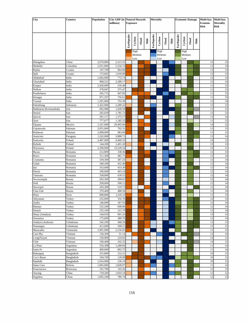
City Country Population City GDP (in
millions)
Multi-haz.
Econom.
Risk
Multi-haz.
Mortality
Risk
Ea
rth
qu
ak
e
Cy
clo
ne
Flo
od
Sli
de
Ea
rth
qu
ak
e
Cy
clo
ne
Flo
od
Sli
de
Ea
rth
qu
ak
e
Cy
clo
ne
Flo
od
Sli
de
3 High 3 High 3 High
2 Medium 2 Medium 2 Medium
1 Low 1 Low 1 Low
Natural Hazards
Exposure
Mortality Economic Damage
Zhengzhou China 2,070,000 2,315.55 0 0 3 2 0 0 3 2 0 0 3 2 13 13
Medellin Colombia 2,951,000 5,534.74 2 0 2 3 3 0 3 3 3 0 2 3 12 14
Rijeka Croatia 147,709 964.68 2 0 3 3 3 0 1 3 3 0 2 3 13 13
Split Croatia 173,692 1,018.89 2 0 3 3 3 0 2 3 3 0 2 3 13 13
Allahabad India 1,062,000 772.74 0 0 3 0 0 0 3 0 0 0 3 0 12 14
Ghaziabad India 968,521 2,288.17 1 0 3 0 3 0 3 0 3 0 3 0 12 14
Kanpur India 2,450,000 550.40 0 0 3 0 0 0 3 0 0 0 3 0 11 15
Nellore India 378,947 375.47 0 3 3 0 0 3 3 0 0 2 2 0 11 15
Pondicherry India 505,715 947.85 0 2 2 2 0 3 2 3 0 3 2 2 11 15
Srinagar India 971,357 750.61 2 0 3 3 3 0 3 3 2 0 3 3 11 15
Varnasi India 1,291,000 755.39 0 0 3 0 0 0 3 0 0 0 3 0 12 14
Palembang Indonesia 1,422,000 2,289.22 1 0 3 0 2 0 3 0 2 0 3 0 13 13
Bakhtaran (Kermanshah) Iran 692,986 1,028.58 3 0 3 3 3 0 3 3 3 0 2 4 11 15
Dezful Iran 202,639 1,785.72 3 0 3 0 3 0 3 0 3 0 3 0 13 13
Qazvin Iran 291,117 1,373.17 3 0 0 2 3 0 0 1 3 0 0 4 12 14
Qom Iran 777,677 1,185.52 3 0 2 0 3 0 3 0 3 0 1 0 11 15
Tijuana Mexico 1,167,000 29,495.84 2 0 2 2 3 0 3 1 3 0 3 1 14 12
Gujranwala Pakistan 2,051,000 792.31 2 0 3 0 3 0 3 0 2 0 3 0 11 15
Peshawar Pakistan 2,098,000 983.60 2 0 3 3 3 0 3 3 2 0 3 3 11 15
Asuncion Paraguay 1,262,000 3,888.71 0 0 3 2 0 0 3 2 0 0 3 2 12 14
Kattowitz Poland 3,487,000 6,460.53 0 0 3 0 0 0 3 0 0 0 3 0 14 12
Rybnik Poland 144,200 1,401.20 1 0 2 0 3 0 1 0 3 0 2 0 13 13
Warszawa Poland 2,269,000 15,529.34 0 0 3 0 0 0 3 0 0 0 3 0 15 11
Bacau Romania 212,800 338.46 3 0 3 2 3 0 2 2 3 0 2 3 12 14
Braov Romania 311,300 485.75 2 0 3 3 3 0 2 3 3 0 2 3 12 14
Constanta Romania 339,300 587.25 1 0 3 0 3 0 2 0 3 0 2 0 12 14
Galati Romania 340,200 432.48 2 0 3 0 3 0 3 0 3 0 3 0 12 14
Iasi Romania 353,600 433.30 2 0 3 2 3 0 2 3 3 0 2 3 12 14
Piteoti Romania 190,600 403.24 2 0 3 0 3 0 2 0 3 0 2 0 12 14
Timioara Romania 338,900 630.55 2 0 3 0 3 0 2 0 3 0 2 0 12 14
Novorossijsk Russia 203,300 399.61 2 0 3 0 3 0 1 0 3 0 2 0 12 14
Sodi Russia 358,600 508.12 2 0 3 0 3 0 2 0 3 0 2 0 12 14
Stavropol Russia 343,300 510.73 2 0 0 2 3 0 0 3 3 0 0 3 12 14
Ulan-Ude Russia 370,400 488.56 1 0 3 0 3 0 2 0 3 0 2 0 12 14
Hims Syria 698,800 1,220.32 2 0 2 0 3 0 3 0 3 0 1 0 11 15
Adiyaman Turkey 232,000 332.76 3 0 3 3 3 0 2 3 3 0 2 3 12 14
Aydin Turkey 146,000 187.93 3 0 3 3 3 0 1 3 2 0 2 3 12 14
Batman Turkey 232,200 608.86 2 0 3 2 3 0 1 3 3 0 2 3 12 14
Denizli Turkey 255,100 315.79 3 0 2 3 3 0 1 3 3 0 1 3 12 14
Hatay (Antakya) Turkey 144,910 691.26 3 0 2 3 3 0 1 3 3 0 1 3 13 13
Osmaniye Turkey 175,600 389.70 3 0 2 3 3 0 1 3 3 0 1 3 12 14
Andijon (Andizan) Uzbekistan 342,200 468.26 3 0 3 2 1 0 3 2 2 0 3 3 13 13
Namangan Uzbekistan 413,600 508.21 3 0 3 2 1 0 3 3 2 0 3 3 13 13
Maracaibo Venezuela 1,901,000 2,256.95 2 0 3 0 3 0 3 0 2 0 3 0 11 15
Cam Pha Vietnam 136,300 51.14 0 2 3 2 0 2 3 3 0 3 3 4 12 14
LongÿXuyen Vietnam 150,900 224.92 0 0 3 0 0 0 3 0 0 0 3 0 14 12
Vinh Vietnam 100,400 242.35 0 1 3 2 0 1 3 3 0 3 3 4 14 12
La Plata Argentina 556,308 1,288.84 0 0 3 0 0 0 3 0 0 0 3 0 11 14
Santa Fe Argentina 400,000 803.75 0 0 3 0 0 0 3 0 0 0 3 0 11 14
Bakerganj Bangladesh 255,800 232.51 0 3 3 0 0 3 3 0 0 2 2 0 10 15
Cox's Bazar Bangladesh 104,700 128.89 2 3 3 3 2 2 3 3 1 2 2 2 10 15
Rajshahi Bangladesh 1,016,000 236.19 1 0 3 0 3 0 3 0 2 0 3 0 10 15
Santa Cruz Bolivia 1,065,000 1,828.07 1 0 3 2 2 0 3 2 2 0 3 2 11 14
Francistown Botswana 101,700 143.26 0 0 2 0 0 0 3 0 0 0 3 0 12 13
Anyang China 718,200 1,810.54 1 0 3 2 2 0 3 2 2 0 3 2 13 12
Jingzhou China 1,065,100 786.74 0 0 3 0 0 0 3 0 0 0 3 0 12 13
116
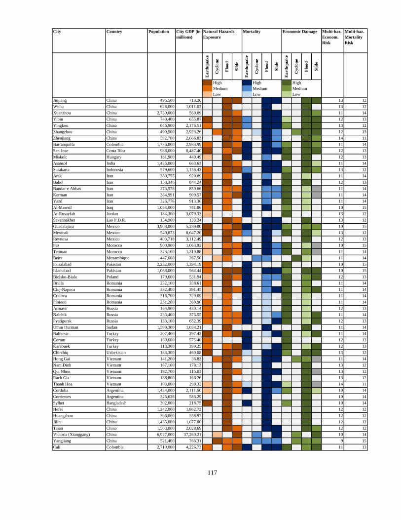
City Country Population City GDP (in
millions)
Multi-haz.
Econom.
Risk
Multi-haz.
Mortality
Risk
Ea
rth
qu
ak
e
Cy
clo
ne
Flo
od
Sli
de
Ea
rth
qu
ak
e
Cy
clo
ne
Flo
od
Sli
de
Ea
rth
qu
ak
e
Cy
clo
ne
Flo
od
Sli
de
3 High 3 High 3 High
2 Medium 2 Medium 2 Medium
1 Low 1 Low 1 Low
Natural Hazards
Exposure
Mortality Economic Damage
Jiujiang China 496,500 713.26 0 0 3 3 0 0 3 3 0 0 3 3 13 12
Wuhu China 628,000 1,011.02 0 0 3 0 0 0 3 0 0 0 3 0 13 12
Xuanzhou China 2,730,000 560.09 0 0 3 2 0 0 3 3 0 0 3 2 11 14
Yibin China 740,400 655.87 3 0 3 3 2 0 3 3 1 0 3 3 12 13
Yingkou China 646,900 2,176.51 2 0 3 3 2 0 3 3 2 0 3 3 13 12
Zhangzhou China 490,500 2,923.26 0 2 3 2 0 1 3 2 0 2 3 3 12 13
Zhenjiang China 592,700 2,666.03 0 0 3 2 0 0 3 2 0 0 3 2 14 11
Barranquilla Colombia 1,736,000 2,933.99 2 0 3 2 3 0 3 2 2 0 3 2 11 14
San Jose Costa Rica 988,000 8,487.40 3 0 2 3 3 0 3 3 3 0 3 3 12 13
Miskolc Hungary 181,900 440.49 1 0 3 0 3 0 2 0 3 0 3 0 12 13
Asansol India 1,425,000 663.63 0 0 3 2 0 0 3 3 0 0 3 1 11 14
Surakarta Indonesia 579,600 1,156.42 2 0 3 3 2 0 3 3 2 0 3 2 13 12
Arak Iran 380,755 920.89 2 0 2 0 3 0 2 0 3 0 1 0 11 14
Babol Iran 158,346 844.24 3 0 3 0 3 0 3 0 3 0 3 0 12 13
Bandar-e Abbas Iran 273,578 859.66 3 0 2 2 3 0 2 2 3 0 1 4 11 14
Kerman Iran 384,991 909.57 3 0 2 3 3 0 2 2 3 0 1 4 11 14
Yazd Iran 326,776 913.36 3 0 2 0 3 0 2 0 3 0 1 0 11 14
Al-Mawsil Iraq 1,034,000 781.86 2 0 2 0 3 0 3 0 2 0 1 0 10 15
Ar-Rusayfah Jordan 184,300 3,079.33 1 0 0 0 3 0 0 0 3 0 0 0 13 12
Savannakhet Lao P.D.R. 154,900 133.24 0 0 3 2 0 0 3 3 0 0 3 0 13 12
Guadalajara Mexico 3,908,000 5,289.00 3 0 2 3 3 0 3 3 2 0 2 2 10 15
Mexicali Mexico 549,873 8,647.26 3 0 3 2 2 0 3 1 3 0 3 1 13 12
Reynosa Mexico 403,718 3,112.49 0 0 3 0 0 0 3 0 0 0 3 0 12 13
Fez Morocco 900,900 1,063.92 1 0 2 2 3 0 3 2 3 0 1 4 10 15
Tetouan Morocco 323,100 1,310.88 1 0 3 2 3 0 3 2 3 0 2 4 11 14
Beira Mozambique 447,600 267.50 0 1 2 0 0 2 2 0 0 3 1 0 11 14
Faisalabad Pakistan 2,232,000 1,394.19 2 0 0 0 3 0 0 0 3 0 0 0 10 15
Islamabad Pakistan 1,068,000 564.44 2 0 3 3 3 0 3 3 2 0 3 3 10 15
Bielsko-Biala Poland 179,600 531.94 1 0 3 2 3 0 2 2 3 0 2 3 12 13
Braila Romania 232,100 338.61 2 0 3 0 3 0 2 0 3 0 2 0 11 14
Cluj-Napoca Romania 332,400 391.45 1 0 3 2 3 0 2 3 3 0 2 3 11 14
Craiova Romania 316,700 329.09 1 0 2 0 3 0 1 0 3 0 1 0 11 14
Ploieoti Romania 251,200 369.90 2 0 2 0 3 0 1 0 3 0 1 0 11 14
Armavir Russia 164,900 430.14 2 0 2 0 3 0 1 0 3 0 1 0 12 13
Nalchik Russia 233,400 376.55 2 0 2 2 3 0 1 2 3 0 1 3 11 14
Pyatigorsk Russia 133,100 652.39 2 0 2 2 3 0 1 3 3 0 1 3 12 13
Umm Durman Sudan 1,599,300 1,034.21 0 0 3 0 0 0 3 0 0 0 3 0 11 14
Balikesir Turkey 207,400 297.42 3 0 2 3 3 0 1 3 3 0 1 3 11 14
Corum Turkey 160,600 575.46 2 0 0 0 3 0 0 0 3 0 0 0 12 13
Karabuek Turkey 113,300 399.25 2 0 2 3 3 0 1 3 3 0 1 3 12 13
Chirchiq Uzbekistan 183,300 460.08 3 0 3 3 1 0 3 3 2 0 3 3 13 12
Hong Gai Vietnam 141,200 36.83 0 2 3 2 0 1 3 3 0 2 2 4 11 14
Nam Dinh Vietnam 187,100 178.13 0 0 3 0 0 0 3 0 0 0 3 0 13 12
Qui Nhon Vietnam 192,700 115.03 0 0 3 2 0 0 3 3 0 0 3 4 13 12
Rach Gia Vietnam 188,800 166.26 0 0 3 0 0 0 3 0 0 0 3 0 13 12
Thanh Hoa Vietnam 103,000 298.33 1 0 3 2 1 0 3 3 1 0 3 4 14 11
Cordoba Argentina 1,434,000 2,111.50 1 0 3 2 3 0 3 2 2 0 3 1 10 14
Corrientes Argentina 325,628 586.29 0 0 3 0 0 0 3 0 0 0 3 0 10 14
Sylhet Bangladesh 302,000 218.75 3 0 3 0 3 0 3 0 2 0 3 0 10 14
Hefei China 1,242,000 1,862.72 0 0 3 0 0 0 3 0 0 0 3 0 12 12
Huangzhou China 366,000 558.97 0 0 3 0 0 0 3 0 0 0 3 0 12 12
Jilin China 1,435,000 1,677.00 0 0 3 0 0 0 3 0 0 0 3 0 12 12
Taian China 1,503,000 2,028.69 0 0 3 2 0 0 3 3 0 0 3 2 12 12
Victoria (Xianggang) China 6,927,000 37,260.21 0 1 0 3 0 2 0 3 0 2 0 3 10 14
Yangjiang China 521,400 766.31 0 3 2 2 0 2 2 2 0 2 2 2 9 15
Cali Colombia 2,710,000 4,226.73 2 0 2 3 3 0 3 3 3 0 2 3 11 13
117
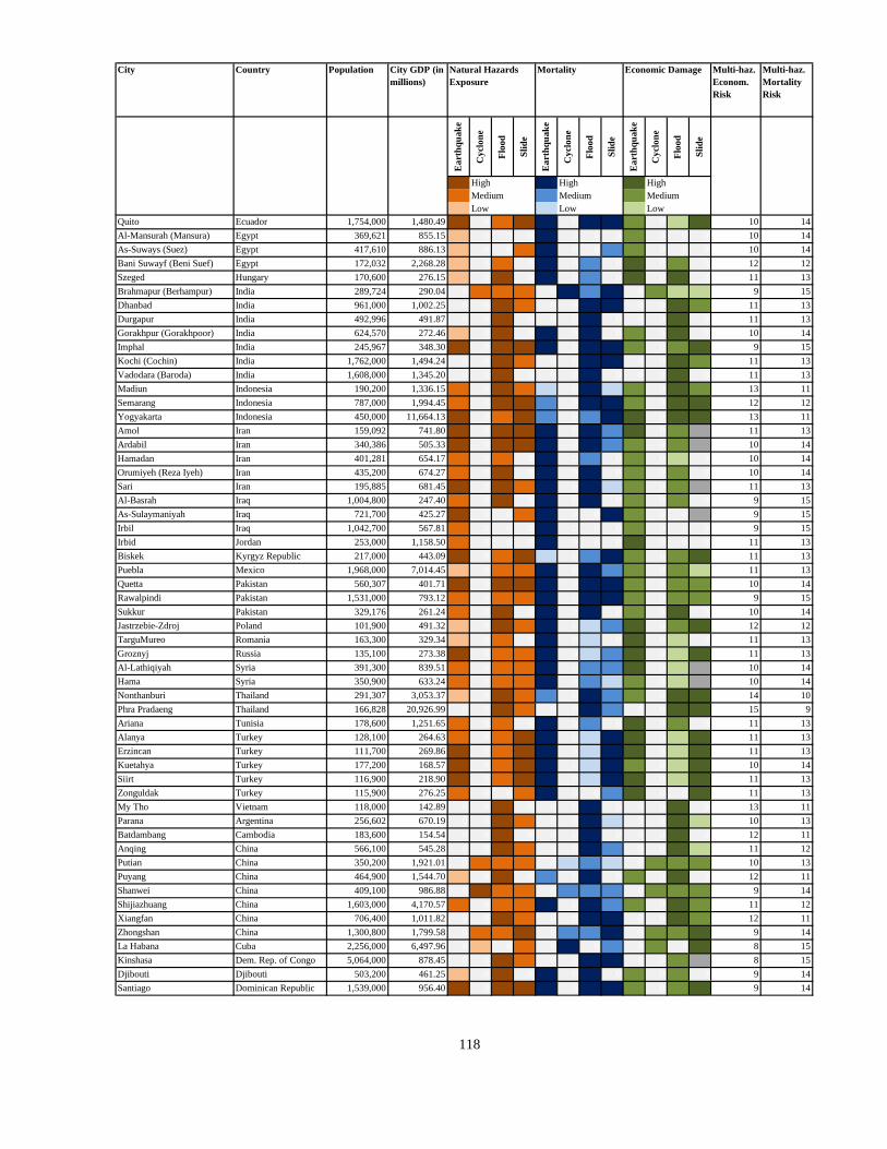
City Country Population City GDP (in
millions)
Multi-haz.
Econom.
Risk
Multi-haz.
Mortality
Risk
Ea
rth
qu
ak
e
Cy
clo
ne
Flo
od
Sli
de
Ea
rth
qu
ak
e
Cy
clo
ne
Flo
od
Sli
de
Ea
rth
qu
ak
e
Cy
clo
ne
Flo
od
Sli
de
3 High 3 High 3 High
2 Medium 2 Medium 2 Medium
1 Low 1 Low 1 Low
Natural Hazards
Exposure
Mortality Economic Damage
Quito Ecuador 1,754,000 1,480.49 3 0 2 3 3 0 3 3 2 0 1 3 10 14
Al-Mansurah (Mansura) Egypt 369,621 855.15 1 0 0 0 3 0 0 0 2 0 0 0 10 14
As-Suways (Suez) Egypt 417,610 886.13 1 0 0 2 3 0 0 2 2 0 0 0 10 14
Bani Suwayf (Beni Suef) Egypt 172,032 2,268.28 1 0 2 0 3 0 2 0 3 0 2 0 12 12
Szeged Hungary 170,600 276.15 1 0 3 0 3 0 2 0 3 0 3 0 11 13
Brahmapur (Berhampur) India 289,724 290.04 0 2 2 2 0 3 2 3 0 2 1 1 9 15
Dhanbad India 961,000 1,002.25 0 0 3 2 0 0 3 3 0 0 3 2 11 13
Durgapur India 492,996 491.87 0 0 3 0 0 0 3 0 0 0 3 0 11 13
Gorakhpur (Gorakhpoor) India 624,570 272.46 1 0 3 0 3 0 3 0 2 0 3 0 10 14
Imphal India 245,967 348.30 3 0 3 3 3 0 3 3 2 0 2 3 9 15
Kochi (Cochin) India 1,762,000 1,494.24 0 0 3 2 0 0 3 3 0 0 3 2 11 13
Vadodara (Baroda) India 1,608,000 1,345.20 0 0 3 0 0 0 3 0 0 0 3 0 11 13
Madiun Indonesia 190,200 1,336.15 2 0 3 2 1 0 3 1 2 0 3 2 13 11
Semarang Indonesia 787,000 1,994.45 2 0 3 3 2 0 3 3 2 0 3 3 12 12
Yogyakarta Indonesia 450,000 11,664.13 3 0 2 3 2 0 2 3 3 0 3 3 13 11
Amol Iran 159,092 741.80 3 0 3 3 3 0 3 2 3 0 2 4 11 13
Ardabil Iran 340,386 505.33 3 0 3 3 3 0 3 2 2 0 2 4 10 14
Hamadan Iran 401,281 654.17 2 0 2 0 3 0 2 0 2 0 1 0 10 14
Orumiyeh (Reza Iyeh) Iran 435,200 674.27 2 0 3 0 3 0 3 0 2 0 2 0 10 14
Sari Iran 195,885 681.45 3 0 3 2 3 0 3 1 2 0 2 4 11 13
Al-Basrah Iraq 1,004,800 247.40 2 0 3 0 3 0 3 0 2 0 2 0 9 15
As-Sulaymaniyah Iraq 721,700 425.27 3 0 0 2 3 0 0 3 2 0 0 4 9 15
Irbil Iraq 1,042,700 567.81 2 0 0 0 3 0 0 0 2 0 0 0 9 15
Irbid Jordan 253,000 1,158.50 2 0 0 0 3 0 0 0 3 0 0 0 11 13
Biskek Kyrgyz Republic 217,000 443.09 3 0 2 3 1 0 2 3 2 0 2 3 11 13
Puebla Mexico 1,968,000 7,014.45 1 0 2 2 3 0 3 2 2 0 2 1 11 13
Quetta Pakistan 560,307 401.71 3 0 3 3 3 0 3 3 2 0 2 2 10 14
Rawalpindi Pakistan 1,531,000 793.12 2 0 2 2 3 0 3 3 2 0 2 2 9 15
Sukkur Pakistan 329,176 261.24 2 0 3 0 3 0 3 0 2 0 3 0 10 14
Jastrzebie-Zdroj Poland 101,900 491.32 1 0 3 2 3 0 1 2 3 0 2 3 12 12
TarguMureo Romania 163,300 329.34 1 0 2 0 3 0 1 0 3 0 1 0 11 13
Groznyj Russia 135,100 273.38 3 0 2 2 3 0 1 2 3 0 1 3 11 13
Al-Lathiqiyah Syria 391,300 839.51 2 0 2 2 3 0 2 2 3 0 1 4 10 14
Hama Syria 350,900 633.24 2 0 2 2 3 0 2 1 2 0 1 4 10 14
Nonthanburi Thailand 291,307 3,053.37 1 0 3 2 2 0 3 2 2 0 3 3 14 10
Phra Pradaeng Thailand 166,828 20,926.99 0 0 3 2 0 0 3 2 0 0 3 3 15 9
Ariana Tunisia 178,600 1,251.65 2 0 2 0 3 0 2 0 3 0 2 0 11 13
Alanya Turkey 128,100 264.63 2 0 2 3 3 0 1 3 3 0 1 3 11 13
Erzincan Turkey 111,700 269.86 3 0 2 3 3 0 1 3 3 0 1 3 11 13
Kuetahya Turkey 177,200 168.57 3 0 2 3 3 0 1 3 2 0 1 3 10 14
Siirt Turkey 116,900 218.90 3 0 2 3 3 0 1 3 3 0 1 3 11 13
Zonguldak Turkey 115,900 276.25 2 0 0 2 3 0 0 2 3 0 0 3 11 13
My Tho Vietnam 118,000 142.89 0 0 3 0 0 0 3 0 0 0 3 0 13 11
Parana Argentina 256,602 670.19 0 0 3 2 0 0 3 1 0 0 3 1 10 13
Batdambang Cambodia 183,600 154.54 0 0 3 0 0 0 3 0 0 0 3 0 12 11
Anqing China 566,100 545.28 0 0 3 2 0 0 3 2 0 0 3 1 11 12
Putian China 350,200 1,921.01 0 2 2 2 0 1 2 1 0 2 2 2 10 13
Puyang China 464,900 1,544.70 1 0 3 0 2 0 3 0 2 0 3 0 12 11
Shanwei China 409,100 986.88 0 3 2 2 0 2 2 2 0 2 2 2 9 14
Shijiazhuang China 1,603,000 4,170.57 2 0 2 2 3 0 3 2 2 0 3 2 11 12
Xiangfan China 706,400 1,011.82 0 0 3 2 0 0 3 3 0 0 3 2 12 11
Zhongshan China 1,300,800 1,799.58 0 2 2 3 0 2 2 3 0 2 2 3 9 14
La Habana Cuba 2,256,000 6,497.96 0 1 0 2 0 3 0 2 0 2 0 3 8 15
Kinshasa Dem. Rep. of Congo 5,064,000 878.45 0 0 3 2 0 0 3 3 0 0 2 4 8 15
Djibouti Djibouti 503,200 461.25 1 0 3 0 3 0 3 0 2 0 2 0 9 14
Santiago Dominican Republic 1,539,000 956.40 3 0 3 3 3 0 3 3 2 0 2 3 9 14
118

City Country Population City GDP (in
millions)
Multi-haz.
Econom.
Risk
Multi-haz.
Mortality
Risk
Ea
rth
qu
ak
e
Cy
clo
ne
Flo
od
Sli
de
Ea
rth
qu
ak
e
Cy
clo
ne
Flo
od
Sli
de
Ea
rth
qu
ak
e
Cy
clo
ne
Flo
od
Sli
de
3 High 3 High 3 High
2 Medium 2 Medium 2 Medium
1 Low 1 Low 1 Low
Natural Hazards
Exposure
Mortality Economic Damage
Al-Isma'iliyah (Ismailia) Egypt 254,477 817.66 1 0 0 0 3 0 0 0 2 0 0 0 10 13
Al-Mahallah Al-Kubra Egypt 395,402 464.26 1 0 0 0 3 0 0 0 2 0 0 0 9 14
Gyoer Hungary 132,000 294.53 1 0 2 0 3 0 1 0 3 0 1 0 10 13
Agartala India 189,327 239.18 3 0 3 0 3 0 3 0 2 0 3 0 10 13
Agra India 1,169,000 628.88 1 0 2 0 3 0 3 0 2 0 1 0 9 14
Bhavnagar (Bhaunagar) India 517,578 378.37 0 1 3 0 0 2 3 0 0 1 2 0 9 14
Faizabad (New Township) India 1,051,000 142.71 1 0 3 0 3 0 3 0 1 0 2 0 8 15
Guntur India 514,707 487.55 1 0 3 0 3 0 3 0 2 0 2 0 9 14
Gwalior India 898,000 390.14 0 0 3 2 0 0 3 3 0 0 3 1 10 13
Jalandhar (Jullundur) India 701,223 645.30 2 0 2 0 3 0 2 0 2 0 1 0 9 14
Kakinada India 368,672 356.35 0 2 2 0 0 2 2 0 0 2 1 0 8 15
Rajahmundry India 408,341 641.71 0 0 3 2 0 0 3 3 0 0 3 1 11 12
Sangli (-Miraj) India 447,632 1,410.14 1 0 2 2 3 0 2 3 2 0 2 2 10 13
Shiliguri (Siliguri) India 470,275 386.08 2 0 3 3 3 0 3 3 2 0 2 2 9 14
Medan Indonesia 1,879,000 4,800.28 2 0 2 0 3 0 3 0 2 0 3 0 11 12
Bander-e Bushehr Iran 143,641 527.13 2 0 3 0 3 0 3 0 2 0 2 0 10 13
Borujerd Iran 217,804 292.70 3 0 3 2 3 0 3 1 2 0 2 4 9 14
Gorgan Iran 188,710 591.75 3 0 2 2 3 0 2 1 2 0 1 4 10 13
Kashan Iran 201,372 539.67 3 0 2 3 3 0 2 2 2 0 1 4 10 13
Khorramshahr (Khuninshahr) Iran 105,636 610.53 2 0 3 0 3 0 3 0 2 0 3 0 11 12
Qa'emshahr Iran 143,286 721.39 3 0 2 0 3 0 2 0 3 0 1 0 10 13
Zahedan Iran 419,518 479.96 3 0 0 0 3 0 0 0 2 0 0 0 9 14
Zanjan Iran 286,295 459.04 3 0 2 3 3 0 2 2 2 0 1 4 9 14
Az-Zubayr Iraq 153,200 378.92 2 0 3 0 3 0 3 0 2 0 2 0 10 13
Tuxtla Gutierrez Mexico 424,579 1,370.91 3 0 3 3 2 0 3 2 2 0 3 1 10 13
Villahermosa Mexico 330,846 1,866.60 1 0 3 0 2 0 3 0 2 0 3 0 11 12
Casablanca Morocco 3,541,000 3,351.21 0 0 3 0 0 0 3 0 0 0 3 0 10 13
Meknes Morocco 545,800 523.56 1 0 0 0 3 0 0 0 2 0 0 0 9 14
Sialkot (incl. Cantonment) Pakistan 417,597 325.27 2 0 3 0 3 0 3 0 2 0 2 0 9 14
Ciudad de Panama Panama 1,173,000 5,144.91 2 0 2 3 3 0 3 3 2 0 2 2 10 13
Dagupan Philippines 130,328 423.85 2 2 3 0 1 1 3 0 1 1 3 0 11 12
Davao Philippines 1,202,000 199.37 3 0 3 3 3 0 3 3 1 0 3 2 9 14
Arad Romania 181,900 199.51 1 0 3 0 3 0 2 0 2 0 2 0 10 13
Buzau Romania 147,600 175.50 3 0 2 2 3 0 1 2 2 0 1 3 10 13
Piatra Neamt Romania 122,800 143.45 2 0 3 2 3 0 2 2 2 0 2 3 10 13
Satu Mare Romania 127,900 209.96 1 0 3 0 3 0 1 0 2 0 2 0 10 13
Berkessk Russia 121,700 182.82 2 0 2 2 3 0 1 2 2 0 1 3 10 13
Juano-Sachalinsk Russia 179,200 283.13 1 0 2 2 3 0 1 2 3 0 1 3 10 13
Kislovodsk Russia 110,000 186.89 2 0 2 2 3 0 1 2 2 0 1 3 10 13
Nevinnomyssk Russia 132,600 246.73 2 0 2 0 3 0 1 0 3 0 1 0 10 13
Beograd (Belgrad) Serbia and Monten. 1,482,000 613.40 2 0 3 2 1 0 3 3 2 0 3 4 12 11
Khujand (Leninabad) Tajikistan 205,200 156.09 3 0 3 2 1 0 3 3 2 0 3 3 11 12
Dar es Salaam Tanzania 2,347,000 1,517.74 0 0 3 2 0 0 3 3 0 0 3 4 9 14
Thanya Buri Thailand 113,818 3,813.30 1 0 3 0 1 0 3 0 2 0 3 14 9
Bismil Turkey 110,700 161.94 2 0 3 0 3 0 1 0 2 0 1 0 10 13
Karaman Turkey 113,700 417.17 1 0 2 0 3 0 1 0 3 0 1 0 11 12
Kiziltepe Turkey 122,300 223.50 2 0 0 0 3 0 0 0 2 0 0 0 10 13
Ordu Turkey 128,500 213.99 2 0 2 2 3 0 1 2 2 0 1 3 10 13
Viransehir Turkey 116,100 228.04 2 0 0 0 3 0 0 0 2 0 0 0 10 13
Kabul Afghanistan 2,590,000 228.26 2 0 2 0 3 0 3 0 2 0 1 0 7 15
Concordia Argentina 131,716 837.57 0 0 3 2 0 0 3 1 0 0 3 1 10 12
Baki (Baku) Azerbaijan 1,936,000 2,445.84 2 0 3 0 1 0 3 0 2 0 3 0 13 9
Brahman Baria Bangladesh 202,400 120.88 2 0 3 0 3 0 3 0 1 0 2 0 9 13
Chandpur Bangladesh 119,900 65.41 1 2 3 0 2 2 3 0 1 1 2 0 8 14
Mymensingh (Nasirabad) Bangladesh 328,400 90.06 2 0 3 0 3 0 3 0 1 0 2 0 8 14
Rangpur Bangladesh 262,300 210.94 2 0 3 0 3 0 3 0 2 0 2 0 9 13
119
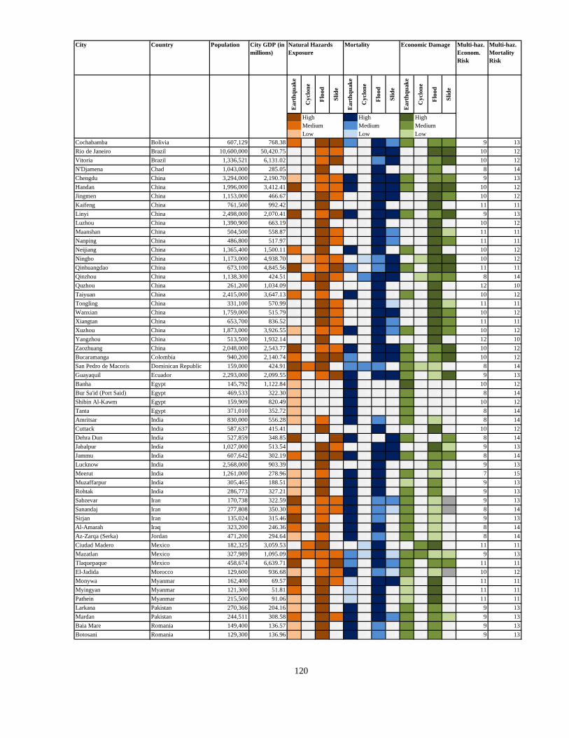
City Country Population City GDP (in
millions)
Multi-haz.
Econom.
Risk
Multi-haz.
Mortality
Risk
Ea
rth
qu
ak
e
Cy
clo
ne
Flo
od
Sli
de
Ea
rth
qu
ak
e
Cy
clo
ne
Flo
od
Sli
de
Ea
rth
qu
ak
e
Cy
clo
ne
Flo
od
Sli
de
3 High 3 High 3 High
2 Medium 2 Medium 2 Medium
1 Low 1 Low 1 Low
Natural Hazards
Exposure
Mortality Economic Damage
Cochabamba Bolivia 607,129 768.38 2 0 3 3 2 0 3 2 2 0 2 2 9 13
Rio de Janeiro Brazil 10,600,000 50,420.75 0 0 2 2 0 0 3 3 0 0 3 3 10 12
Vitoria Brazil 1,336,521 6,131.02 0 0 2 3 0 0 2 3 0 0 2 3 10 12
N'Djamena Chad 1,043,000 285.05 0 0 3 0 0 0 3 0 0 0 2 0 8 14
Chengdu China 3,294,000 2,190.70 1 0 2 2 3 0 3 3 2 0 2 2 9 13
Handan China 1,996,000 3,412.41 3 0 2 2 3 0 3 3 2 0 3 3 10 12
Jingmen China 1,153,000 466.67 0 0 3 2 0 0 3 3 0 0 3 2 10 12
Kaifeng China 761,500 992.42 0 0 3 0 0 0 3 0 0 0 3 0 11 11
Linyi China 2,498,000 2,070.41 3 0 2 3 3 0 3 3 2 0 2 3 9 13
Luzhou China 1,390,900 663.19 0 0 3 0 0 0 3 0 0 0 3 0 10 12
Maanshan China 504,500 558.87 0 0 3 2 0 0 3 2 0 0 3 1 11 11
Nanping China 486,800 517.97 0 0 3 2 0 0 3 2 0 0 3 2 11 11
Neijiang China 1,365,400 1,500.11 2 0 3 0 3 0 3 0 2 0 3 0 10 12
Ningbo China 1,173,000 4,938.70 0 1 2 2 0 1 2 3 0 1 3 3 10 12
Qinhuangdao China 673,100 4,845.56 3 0 2 3 2 0 2 3 2 0 3 3 11 11
Qinzhou China 1,138,300 424.51 0 2 3 2 0 2 3 3 0 1 2 2 8 14
Quzhou China 261,200 1,034.09 0 0 3 0 0 0 3 0 0 0 3 0 12 10
Taiyuan China 2,415,000 3,647.13 2 0 2 0 3 0 3 0 2 0 3 0 10 12
Tongling China 331,100 570.99 0 0 3 2 0 0 3 1 0 0 3 1 11 11
Wanxian China 1,759,000 515.79 0 0 3 2 0 0 3 3 0 0 3 2 10 12
Xiangtan China 653,700 836.52 0 0 3 2 0 0 3 2 0 0 3 2 11 11
Xuzhou China 1,873,000 3,926.55 1 0 2 2 3 0 3 2 2 0 3 2 10 12
Yangzhou China 513,500 1,932.14 0 0 3 0 0 0 3 0 0 0 3 0 12 10
Zaozhuang China 2,048,000 2,543.77 3 0 2 2 3 0 3 3 2 0 2 3 10 12
Bucaramanga Colombia 940,200 2,140.74 2 0 3 3 2 0 3 3 2 0 2 3 10 12
San Pedro de Macoris Dominican Republic 159,000 424.91 3 2 3 0 2 2 2 0 2 1 1 0 8 14
Guayaquil Ecuador 2,293,000 2,099.55 2 0 2 3 3 0 3 3 2 0 1 3 9 13
Banha Egypt 145,792 1,122.84 1 0 0 0 3 0 0 0 3 0 0 0 10 12
Bur Sa'id (Port Said) Egypt 469,533 322.30 1 0 0 0 3 0 0 0 2 0 0 0 8 14
Shibin Al-Kawm Egypt 159,909 820.49 1 0 0 0 3 0 0 0 2 0 0 0 10 12
Tanta Egypt 371,010 352.72 1 0 0 0 3 0 0 0 2 0 0 0 8 14
Amritsar India 830,000 556.28 1 0 2 0 3 0 2 0 2 0 1 0 8 14
Cuttack India 587,637 415.41 0 0 3 0 0 0 3 0 0 0 3 0 10 12
Dehra Dun India 527,859 348.85 3 0 0 3 3 0 0 3 2 0 0 2 8 14
Jabalpur India 1,027,000 513.54 0 0 3 2 0 0 3 3 0 0 3 1 9 13
Jammu India 607,642 302.19 2 0 3 3 3 0 3 3 2 0 2 2 8 14
Lucknow India 2,568,000 903.39 0 0 3 0 0 0 3 0 0 0 2 0 9 13
Meerut India 1,261,000 278.96 1 0 2 0 3 0 3 0 2 0 1 0 7 15
Muzaffarpur India 305,465 188.51 1 0 3 0 3 0 3 0 1 0 2 0 9 13
Rohtak India 286,773 327.21 1 0 3 0 3 0 3 0 2 0 2 0 9 13
Sabzevar Iran 170,738 322.59 3 0 2 2 3 0 2 2 2 0 1 4 9 13
Sanandaj Iran 277,808 350.30 2 0 2 2 3 0 2 1 2 0 1 4 8 14
Sirjan Iran 135,024 315.46 3 0 2 0 3 0 2 0 2 0 1 0 9 13
Al-Amarah Iraq 323,200 246.36 2 0 3 0 3 0 3 0 2 0 1 0 8 14
Az-Zarqa (Serka) Jordan 471,200 294.64 1 0 2 0 3 0 2 0 2 0 1 0 8 14
Ciudad Madero Mexico 182,325 3,059.53 0 2 3 0 0 1 3 0 0 2 3 0 11 11
Mazatlan Mexico 327,989 1,095.09 2 2 2 2 2 1 3 1 2 2 1 1 9 13
Tlaquepaque Mexico 458,674 6,639.71 3 0 2 3 2 0 3 2 2 0 2 2 11 11
El-Jadida Morocco 129,600 936.68 1 0 2 2 3 0 2 1 2 0 1 4 10 12
Monywa Myanmar 162,400 69.57 3 0 3 2 1 0 3 3 1 0 3 0 11 11
Myingyan Myanmar 121,300 51.81 2 0 3 0 1 0 3 0 1 0 3 0 11 11
Pathein Myanmar 215,500 91.06 1 0 3 0 1 0 3 0 1 0 3 0 11 11
Larkana Pakistan 270,366 204.16 1 0 3 0 3 0 3 0 2 0 2 0 9 13
Mardan Pakistan 244,511 308.58 2 0 3 2 3 0 3 2 2 0 2 1 9 13
Baia Mare Romania 149,400 136.57 1 0 3 0 3 0 2 0 2 0 2 0 9 13
Botosani Romania 129,300 136.96 1 0 3 0 3 0 2 0 2 0 2 0 9 13
120
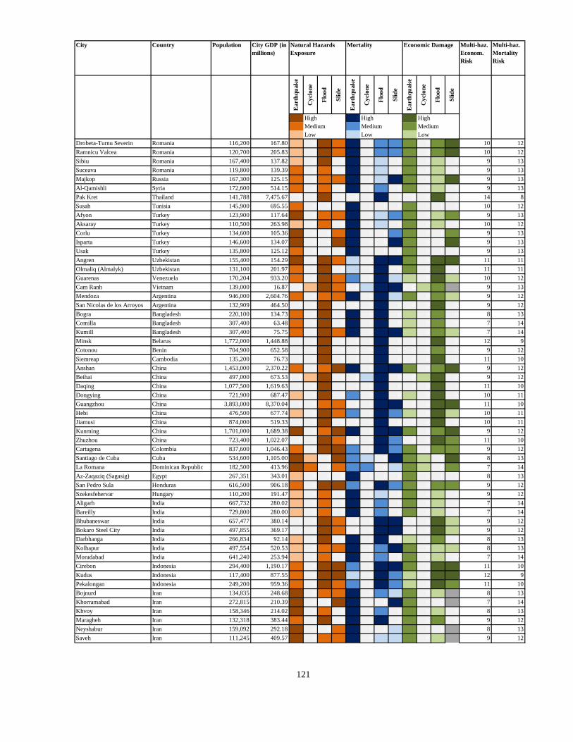
City Country Population City GDP (in
millions)
Multi-haz.
Econom.
Risk
Multi-haz.
Mortality
Risk
Ea
rth
qu
ak
e
Cy
clo
ne
Flo
od
Sli
de
Ea
rth
qu
ak
e
Cy
clo
ne
Flo
od
Sli
de
Ea
rth
qu
ak
e
Cy
clo
ne
Flo
od
Sli
de
3 High 3 High 3 High
2 Medium 2 Medium 2 Medium
1 Low 1 Low 1 Low
Natural Hazards
Exposure
Mortality Economic Damage
Drobeta-Turnu Severin Romania 116,200 167.80 1 0 3 2 3 0 2 2 2 0 2 3 10 12
Ramnicu Valcea Romania 120,700 205.83 1 0 3 2 3 0 2 2 2 0 2 3 10 12
Sibiu Romania 167,400 137.82 1 0 3 0 3 0 1 0 2 0 1 0 9 13
Suceava Romania 119,800 139.39 2 0 2 0 3 0 1 0 2 0 1 0 9 13
Majkop Russia 167,300 125.15 2 0 2 2 3 0 1 3 2 0 1 3 9 13
Al-Qamishli Syria 172,600 514.15 2 0 2 0 3 0 2 0 2 0 1 0 9 13
Pak Kret Thailand 141,788 7,475.67 0 0 3 0 0 0 3 0 0 0 3 0 14 8
Susah Tunisia 145,900 695.55 2 0 0 0 3 0 0 0 2 0 0 0 10 12
Afyon Turkey 123,900 117.64 3 0 2 2 3 0 1 2 2 0 1 2 9 13
Aksaray Turkey 110,500 263.98 1 0 2 0 3 0 1 0 2 0 1 0 10 12
Corlu Turkey 134,600 105.36 3 0 0 2 3 0 0 2 2 0 0 2 9 13
Isparta Turkey 146,600 134.07 3 0 0 3 3 0 0 3 2 0 0 3 9 13
Usak Turkey 135,800 125.12 2 0 0 0 3 0 0 0 2 0 0 0 9 13
Angren Uzbekistan 155,400 154.29 3 0 3 2 1 0 3 3 2 0 3 3 11 11
Olmaliq (Almalyk) Uzbekistan 131,100 201.97 2 0 3 0 1 0 3 0 2 0 3 0 11 11
Guarenas Venezuela 170,204 933.20 2 0 3 2 2 0 3 1 1 0 3 1 10 12
Cam Ranh Vietnam 139,000 16.87 0 1 3 2 0 1 3 3 0 1 2 4 9 13
Mendoza Argentina 946,000 2,604.76 2 0 2 2 3 0 3 1 2 0 2 1 9 12
San Nicolas de los Arroyos Argentina 132,909 464.50 0 0 3 0 0 0 3 0 0 0 3 0 9 12
Bogra Bangladesh 220,100 134.73 2 0 3 0 3 0 3 0 1 0 2 0 8 13
Comilla Bangladesh 307,400 63.48 2 0 3 0 3 0 3 0 1 0 2 0 7 14
Kumill Bangladesh 307,400 75.75 2 0 3 2 3 0 3 3 1 0 2 1 7 14
Minsk Belarus 1,772,000 1,448.88 0 0 3 0 0 0 3 0 0 0 3 0 12 9
Cotonou Benin 704,900 652.58 0 0 3 0 0 0 3 0 0 0 2 0 9 12
Siemreap Cambodia 135,200 76.73 0 0 3 0 0 0 3 0 0 0 3 0 11 10
Anshan China 1,453,000 2,370.22 2 0 2 3 3 0 3 3 2 0 2 3 9 12
Beihai China 497,000 673.53 0 1 3 0 0 1 3 0 0 1 3 0 9 12
Daqing China 1,077,500 1,619.63 0 0 3 0 0 0 3 0 0 0 3 0 11 10
Dongying China 721,900 687.47 1 0 3 0 2 0 3 0 1 0 3 0 10 11
Guangzhou China 3,893,000 8,370.04 0 0 2 2 0 0 3 3 0 0 3 3 11 10
Hebi China 476,500 677.74 1 0 3 2 2 0 3 2 1 0 3 1 10 11
Jiamusi China 874,000 519.33 0 0 3 0 0 0 3 0 0 0 3 0 10 11
Kunming China 1,701,000 1,689.38 3 0 2 3 3 0 3 3 2 0 2 3 9 12
Zhuzhou China 723,400 1,022.07 0 0 3 2 0 0 3 2 0 0 3 2 11 10
Cartagena Colombia 837,600 1,046.43 2 0 3 3 2 0 3 2 2 0 2 2 9 12
Santiago de Cuba Cuba 534,600 1,105.00 3 1 0 3 2 1 0 3 2 1 0 3 8 13
La Romana Dominican Republic 182,500 413.96 3 2 0 2 2 2 0 1 2 1 0 2 7 14
Az-Zaqaziq (Sagasig) Egypt 267,351 343.01 1 0 0 0 3 0 0 0 2 0 0 0 8 13
San Pedro Sula Honduras 616,500 906.18 2 0 3 3 2 0 3 2 2 0 2 2 9 12
Szekesfehervar Hungary 110,200 191.47 1 0 2 0 3 0 1 0 2 0 1 0 9 12
Aligarh India 667,732 280.02 1 0 2 0 3 0 2 0 2 0 1 0 7 14
Bareilly India 729,800 280.00 1 0 2 0 3 0 2 0 2 0 1 0 7 14
Bhubaneswar India 657,477 380.14 0 0 3 2 0 0 3 3 0 0 3 1 9 12
Bokaro Steel City India 497,855 369.17 0 0 3 2 0 0 3 3 0 0 3 1 9 12
Darbhanga India 266,834 92.14 1 0 3 0 3 0 3 0 1 0 2 0 8 13
Kolhapur India 497,554 520.53 1 0 2 2 3 0 2 3 2 0 1 1 8 13
Moradabad India 641,240 253.94 1 0 2 0 3 0 2 0 2 0 1 0 7 14
Cirebon Indonesia 294,400 1,190.17 2 0 3 3 2 0 3 3 2 0 3 3 11 10
Kudus Indonesia 117,400 877.55 2 0 3 3 1 0 3 2 1 0 3 3 12 9
Pekalongan Indonesia 249,200 959.36 2 0 3 2 2 0 3 2 1 0 3 2 11 10
Bojnurd Iran 134,835 248.68 3 0 2 2 3 0 2 1 2 0 1 4 8 13
Khorramabad Iran 272,815 210.39 3 0 0 3 3 0 0 3 2 0 0 4 7 14
Khvoy Iran 158,346 214.02 3 0 2 0 3 0 2 0 2 0 1 0 8 13
Maragheh Iran 132,318 383.44 2 0 3 0 3 0 3 0 2 0 2 0 9 12
Neyshabur Iran 159,092 292.18 3 0 0 2 3 0 0 1 2 0 0 4 8 13
Saveh Iran 111,245 409.57 3 0 2 2 3 0 1 1 2 0 1 4 9 12
121

City Country Population City GDP (in
millions)
Multi-haz.
Econom.
Risk
Multi-haz.
Mortality
Risk
Ea
rth
qu
ak
e
Cy
clo
ne
Flo
od
Sli
de
Ea
rth
qu
ak
e
Cy
clo
ne
Flo
od
Sli
de
Ea
rth
qu
ak
e
Cy
clo
ne
Flo
od
Sli
de
3 High 3 High 3 High
2 Medium 2 Medium 2 Medium
1 Low 1 Low 1 Low
Natural Hazards
Exposure
Mortality Economic Damage
Al-Kut Iraq 352,800 216.02 2 0 2 0 3 0 2 0 2 0 1 0 7 14
Almaty Kazakhstan 1,248,000 2,018.05 3 0 2 3 1 0 1 3 2 0 2 4 10 11
Toamasina Madagascar 166,000 26.83 0 1 2 0 0 1 2 0 0 2 1 0 8 13
Chihuahua Mexico 657,876 2,761.67 0 0 3 0 0 0 3 0 0 0 3 0 9 12
Ciudad Juarez Mexico 1,168,000 22,370.13 0 0 2 0 0 0 3 0 0 0 3 0 11 10
Minatitlan Mexico 109,193 2,370.64 1 0 3 2 1 0 3 1 2 0 3 1 11 10
Monterrey Mexico 3,416,000 9,864.26 0 0 2 2 0 0 3 2 0 0 3 1 9 12
Zapopan Mexico 910,690 3,223.01 3 0 2 3 3 0 3 3 2 0 2 2 9 12
Rabat Morocco 1,496,000 1,796.62 0 0 3 2 0 0 3 2 0 0 3 4 9 12
Pakokku Myanmar 111,100 46.30 2 0 3 0 1 0 3 0 1 0 3 0 10 11
Pyay Myanmar 123,800 49.94 1 0 3 3 1 0 3 3 1 0 3 0 10 11
Kathmandu Nepal 701,499 213.07 3 0 0 3 3 0 0 3 2 0 0 2 7 14
Kano Nigeria 3,169,100 1,102.87 0 0 3 0 0 0 3 0 0 0 2 0 8 13
Gujrat Pakistan 250,121 181.11 2 0 3 0 3 0 3 0 2 0 2 0 8 13
Jhang Sadar Pakistan 292,214 213.48 1 0 3 0 3 0 3 0 2 0 2 0 8 13
Arequipa Peru 720,400 2,329.58 3 0 2 3 2 0 2 2 2 0 1 3 10 11
Angeles Philippines 263,971 277.25 3 0 3 3 2 0 3 2 1 0 3 2 10 11
San Fernando Philippines 102,082 337.26 3 0 3 0 1 0 3 0 1 0 3 0 11 10
Magadan Russia 121,000 88.84 2 0 0 2 3 0 0 2 2 0 0 2 8 13
Usolje-Sibirskoje Russia 103,500 118.99 1 0 3 0 3 0 1 0 2 0 2 0 9 12
Al-Hasakah Syria 185,800 289.42 1 0 3 0 3 0 2 0 2 0 1 0 8 13
Dushanbe Tajikistan 691,600 499.35 3 0 2 3 2 0 3 3 2 0 2 3 10 11
Edirne Turkey 125,600 91.16 2 0 3 0 3 0 1 0 2 0 1 0 8 13
Tekirdag Turkey 109,800 66.69 3 0 3 2 3 0 1 3 2 0 1 3 8 13
Samarqand (Samarkand) Uzbekistan 371,800 536.92 3 0 2 0 1 0 3 0 2 0 2 0 11 10
Ciudad Guayana Venezuela 704,168 1,888.81 1 0 3 2 2 0 3 1 2 0 2 1 9 12
Puerto Cabello Venezuela 169,959 529.72 2 0 3 3 2 0 3 1 1 0 3 1 9 12
Ca Mau Vietnam 101,900 75.85 0 0 3 0 0 0 3 0 0 0 3 0 11 10
Phan Thiet Vietnam 139,200 45.09 0 1 3 2 0 1 3 3 0 1 3 4 10 11
Formosa Argentina 197,057 199.26 0 0 3 0 0 0 3 0 0 0 2 0 7 13
Posadas Argentina 250,000 456.13 0 0 3 2 0 0 3 1 0 0 2 1 8 12
Kushtia Bangladesh 114,100 141.86 1 0 3 0 2 0 3 0 1 0 2 0 9 11
Naogaon Bangladesh 143,700 123.39 2 0 3 0 3 0 3 0 1 0 2 0 8 12
Nawabganj Bangladesh 149,200 131.99 1 0 3 0 2 0 3 0 1 0 2 0 8 12
La Paz Bolivia 1,480,000 1,062.17 2 0 0 2 3 0 0 2 2 0 0 2 8 12
Moji das Cruzes Brazil 116,117 16,073.25 0 0 3 2 0 0 2 1 0 0 3 3 13 7
Baotou China 1,319,000 2,324.51 2 0 2 0 2 0 2 0 2 0 2 0 9 11
Chuzhou China 468,600 243.82 0 0 3 2 0 0 3 2 0 0 3 1 9 11
Fangchenggang China 464,400 218.37 0 2 3 3 0 1 3 3 0 1 2 2 7 13
Heze China 1,600,000 2,471.32 1 0 2 0 2 0 3 0 2 0 2 0 9 11
Hohhot China 978,000 1,564.91 2 0 2 2 2 0 2 2 2 0 2 2 9 11
Jieyang China 624,700 2,629.93 1 0 2 3 2 0 2 3 2 0 2 3 10 10
Lanzhou China 1,730,000 1,405.31 2 0 2 2 3 0 3 2 2 0 2 2 8 12
Sanya China 446,000 219.09 1 3 0 2 0 2 0 2 1 1 0 1 6 14
Shenyang China 4,828,000 4,810.10 0 0 2 0 0 0 3 0 0 0 3 0 10 10
Weifang China 1,287,000 2,198.55 2 0 2 2 2 0 2 2 2 0 2 2 9 11
Weinan China 861,000 620.93 0 0 3 2 0 0 3 2 0 0 3 1 9 11
Zhanjiang China 1,368,000 1,265.00 0 1 0 2 0 2 0 3 0 1 0 2 6 14
Aizawl India 229,714 157.15 3 0 2 3 3 0 2 3 2 0 1 3 6 14
Bhilai (Bhilai Nagar) India 925,000 660.37 0 0 3 0 0 0 3 0 0 0 2 0 9 11
Gandhinagar India 195,891 1,392.37 0 0 3 0 0 0 3 0 0 0 3 0 11 9
Kharagpur India 296,323 354.92 0 0 3 0 0 0 3 0 0 0 3 0 9 11
Patiala India 323,309 297.19 2 0 2 0 3 0 2 0 2 0 1 0 7 13
Raipur India 605,131 653.11 0 0 3 0 0 0 3 0 0 0 2 0 9 11
Shillong India 267,881 240.10 3 0 2 3 3 0 2 3 2 0 1 2 7 13
Thane India 1,484,000 8,944.18 0 0 2 2 0 0 3 3 0 0 3 3 10 10
122
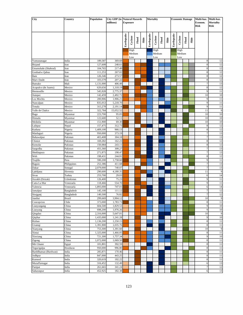
City Country Population City GDP (in
millions)
Multi-haz.
Econom.
Risk
Multi-haz.
Mortality
Risk
Ea
rth
qu
ak
e
Cy
clo
ne
Flo
od
Sli
de
Ea
rth
qu
ak
e
Cy
clo
ne
Flo
od
Sli
de
Ea
rth
qu
ak
e
Cy
clo
ne
Flo
od
Sli
de
3 High 3 High 3 High
2 Medium 2 Medium 2 Medium
1 Low 1 Low 1 Low
Natural Hazards
Exposure
Mortality Economic Damage
Yamunanagar India 189,587 369.69 2 0 0 0 3 0 0 0 2 0 0 0 8 12
Birjand Iran 127,608 248.61 3 0 2 3 3 0 2 2 2 0 1 4 8 12
Emamshahr (Shahrud) Iran 104,765 217.49 3 0 2 2 3 0 1 1 2 0 1 4 8 12
Gonbad-e Qabus Iran 111,253 267.02 3 0 2 2 3 0 1 1 2 0 1 4 8 12
Ilam Iran 126,346 273.57 3 0 0 3 3 0 0 2 2 0 0 4 8 12
Marv Dasht Iran 103,579 207.22 2 0 3 2 3 0 3 1 2 0 2 4 8 12
Bamako Mali 1,131,000 406.49 0 0 3 0 0 0 3 0 0 0 2 0 7 13
Acapulco (de Juarez) Mexico 620,656 1,318.19 3 0 2 3 3 0 3 2 2 0 2 1 8 12
Hermosillo Mexico 545,928 2,775.37 1 0 2 0 2 0 3 0 2 0 2 0 9 11
Jiutepec Mexico 142,459 2,492.72 2 0 3 3 2 0 3 1 2 0 3 1 10 10
Los Mochis Mexico 200,906 1,906.21 2 1 2 2 2 1 2 1 2 1 2 1 9 11
Naucalpan Mexico 835,053 5,218.70 1 0 0 2 2 0 0 2 2 0 0 1 9 11
Tonala Mexico 315,278 2,191.14 3 0 2 3 2 0 3 3 2 0 2 3 9 11
Valle de Chalco Mexico 322,784 15,052.52 1 0 0 2 2 0 0 1 3 0 0 2 11 9
Bago Myanmar 223,700 95.05 2 0 3 0 1 0 3 0 1 0 3 0 10 10
Hintada Myanmar 122,600 52.11 1 0 3 0 1 0 3 0 1 0 3 0 10 10
Meiktila Myanmar 151,900 69.30 3 0 3 0 1 0 3 0 1 0 3 0 10 10
Lalitpur Nepal 157,475 312.73 3 0 0 3 3 0 0 3 2 0 0 2 8 12
Kaduna Nigeria 1,409,100 966.13 0 0 3 0 0 0 3 0 0 0 2 0 8 12
Maiduguri Nigeria 950,000 373.19 0 0 3 0 0 0 3 0 0 0 2 0 7 13
Bahawalpur Pakistan 403,408 304.18 1 0 2 0 3 0 2 0 2 0 1 0 7 13
Chiniot Pakistan 169,282 162.23 2 0 3 0 3 0 3 0 2 0 2 0 8 12
Kemoke Pakistan 150,984 243.11 2 0 3 0 3 0 2 0 2 0 2 0 8 12
Sargodha Pakistan 455,360 308.27 2 0 2 0 3 0 2 0 2 0 1 0 7 13
Shekhapura Pakistan 271,875 198.47 2 0 3 0 3 0 2 0 2 0 1 0 7 13
Weh Pakistan 198,431 244.81 2 0 3 3 3 0 2 3 2 0 2 2 8 12
Trujillo Peru 590,200 1,758.60 3 0 0 2 2 0 0 1 2 0 0 2 9 11
Baguio Philippines 252,386 411.68 2 0 0 3 2 0 0 3 1 0 0 3 7 13
Dakar Senegal 2,079,000 740.07 0 0 3 0 0 0 3 0 0 0 2 0 7 13
Ljubljana Slovenia 290,600 4,180.35 2 0 2 3 2 0 1 3 2 0 2 3 11 9
Sivas Turkey 253,700 29.03 2 0 2 0 3 0 1 0 1 0 1 0 6 14
Jizzakh (Dzizak) Uzbekistan 126,400 75.23 2 0 3 0 1 0 3 0 1 0 3 0 9 11
Catia La Mar Venezuela 118,466 554.70 2 0 3 2 1 0 3 1 1 0 3 1 9 11
Valencia Venezuela 1,893,000 747.01 3 0 2 3 3 0 3 2 1 0 1 1 6 14
Jamalpur Bangladesh 145,100 111.12 3 0 3 0 3 0 3 0 1 0 2 0 7 12
Sirajganj Bangladesh 140,500 76.82 2 0 3 0 3 0 3 0 1 0 2 0 7 12
Jundiai Brazil 299,669 3,904.12 0 0 3 2 0 0 3 1 0 0 3 2 10 9
Concepcion Chile 373,000 1,783.73 3 0 2 2 2 0 3 1 2 0 2 1 8 11
Lianyungang China 604,500 1,829.53 1 0 2 2 2 0 2 2 2 0 2 2 9 10
Liaoyang China 698,200 1,976.26 1 0 2 2 2 0 2 2 2 0 2 2 9 10
Qingdao China 2,316,000 5,647.01 0 0 2 2 0 0 3 3 0 0 3 3 10 9
Qiqihar China 1,435,000 1,241.28 0 0 3 0 0 0 3 0 0 0 3 0 9 10
Rizhao China 1,136,200 1,250.15 2 0 2 0 2 0 2 0 2 0 2 0 8 11
Urumqi China 1,391,900 1,035.76 2 0 2 0 3 0 3 0 2 0 2 0 8 11
Xianyang China 753,300 1,391.60 0 0 3 0 0 0 3 0 0 0 3 0 10 9
Xintai China 1,325,000 1,466.05 2 0 2 2 2 0 2 2 2 0 2 2 8 11
Xinxiang China 721,300 1,757.34 1 0 2 2 2 0 2 3 2 0 2 2 9 10
Zigong China 1,072,000 1,069.50 3 0 2 2 2 0 2 2 2 0 2 2 8 11
Mit Ghamr Egypt 101,801 392.59 1 0 0 0 3 0 0 0 2 0 0 0 8 11
Tegucigalpa Honduras 950,000 996.80 2 0 0 3 2 0 0 3 2 0 0 2 8 11
Barddhaman (Burdwan) India 285,871 170.46 0 0 3 0 0 0 3 0 0 0 2 0 8 11
Jodhpur India 847,000 443.25 0 0 3 0 0 0 3 0 0 0 2 0 8 11
Kurnool India 320,619 192.22 0 0 3 0 0 0 3 0 0 0 2 0 8 11
Muzaffarnagar India 316,452 132.49 1 0 3 0 3 0 3 0 1 0 1 0 6 13
Panipat India 261,665 341.24 1 0 0 0 3 0 0 0 2 0 0 0 7 12
Saharanpur India 452,925 182.38 2 0 0 0 3 0 0 0 2 0 0 0 6 13
123

City Country Population City GDP (in
millions)
Multi-haz.
Econom.
Risk
Multi-haz.
Mortality
Risk
Ea
rth
qu
ak
e
Cy
clo
ne
Flo
od
Sli
de
Ea
rth
qu
ak
e
Cy
clo
ne
Flo
od
Sli
de
Ea
rth
qu
ak
e
Cy
clo
ne
Flo
od
Sli
de
3 High 3 High 3 High
2 Medium 2 Medium 2 Medium
1 Low 1 Low 1 Low
Natural Hazards
Exposure
Mortality Economic Damage
Shimla India 142,161 228.08 3 0 0 3 3 0 0 3 2 0 0 2 7 12
Thiruvananthapuram (Trivandrum)India 1,229,000 1,062.78 0 0 3 0 0 0 3 0 0 0 2 0 8 11
Padang Indonesia 611,900 1,067.11 2 0 0 3 2 0 0 3 2 0 0 3 7 12
Andimeshk Iran 106,923 175.26 3 0 0 2 3 0 0 1 2 0 0 4 7 12
Mahabad Iran 107,799 145.93 2 0 3 0 3 0 3 0 2 0 2 0 7 12
Malayer Iran 144,373 229.34 2 0 2 0 3 0 2 0 2 0 1 0 7 12
Shahr-e Kord Iran 100,477 203.32 2 0 0 0 3 0 0 0 2 0 0 0 7 12
Bacqubah Iraq 256,000 132.83 2 0 2 0 3 0 2 0 2 0 1 0 6 13
Bagdad Iraq 4,797,000 4,903.21 0 0 2 0 0 0 3 0 0 0 2 0 8 11
Oskemen Kyrgyz Republic 793,100 71.01 3 0 2 3 2 0 3 3 1 0 1 3 6 13
Luang Prabang Lao P.D.R. 116,000 116.81 1 0 3 0 1 0 3 0 1 0 3 0 10 9
Culiacan Mexico 540,823 2,053.19 2 0 2 3 2 0 3 1 2 0 2 1 8 11
Oaxaca Mexico 251,846 1,824.15 3 0 2 3 2 0 2 3 2 0 2 3 8 11
San Nicolas de los Garzas Mexico 496,879 16,448.71 0 0 2 2 0 0 3 1 0 0 3 2 10 9
Tlalnepantla Mexico 714,735 4,050.99 1 0 0 2 2 0 0 1 2 0 0 1 8 11
Ulan-Bator Mongolia 738,000 375.14 1 0 2 0 1 0 3 0 1 0 3 0 9 10
Wiratnagar Nepal 168,544 100.04 2 0 3 0 3 0 3 0 1 0 2 0 7 12
Dera Ghozi Khan Pakistan 188,149 140.77 2 0 3 0 3 0 3 0 1 0 2 0 7 12
Marpur Khas Pakistan 184,465 129.06 1 0 3 0 3 0 3 0 1 0 2 0 7 12
Port Moresby Papua New Guinea 300,200 175.80 1 0 2 3 1 0 3 3 1 0 2 0 8 11
Chiclayo Peru 481,100 1,346.22 3 0 0 2 2 0 0 2 2 0 0 2 9 10
Batangas Philippines 247,588 275.73 3 0 3 3 2 0 3 3 1 0 2 3 8 11
Krakow Poland 857,000 2,105.92 0 0 3 0 0 0 3 0 0 0 3 0 11 8
Chelyabinsk Russia 1,185,000 2,959.30 0 0 3 0 0 0 3 0 0 0 3 0 11 8
Kazan Russia 1,137,000 3,221.42 0 0 3 0 0 0 3 0 0 0 3 0 11 8
Samara (Kujbysev) Russia 1,260,000 3,374.71 0 0 3 0 0 0 3 0 0 0 3 0 11 8
Ufa Russia 1,139,000 2,545.87 0 0 3 0 0 0 3 0 0 0 3 0 11 8
Tartus Syria 141,500 226.79 2 0 0 2 3 0 0 1 2 0 0 4 7 12
Kampala Uganda 1,212,000 1,217.07 1 0 2 0 2 0 3 0 2 0 2 0 8 11
Kharkiv (Kharkov, Charkov) Ukraine 1,526,000 1,669.36 0 0 3 0 0 0 2 0 0 0 3 0 12 7
Mazar-i Sharif Afghanistan 232,800 83.98 3 0 2 0 3 0 2 0 1 0 1 0 5 13
Resistencia Argentina 280,000 274.76 0 0 3 0 0 0 3 0 0 0 2 0 6 12
San Miguel de Tucuman Argentina 519,252 1,534.21 2 0 2 3 2 0 3 1 2 0 2 1 7 11
Chudanga Bangladesh 107,900 155.22 1 0 3 0 2 0 2 0 1 0 2 0 7 11
Pabna Bangladesh 154,500 125.62 1 0 3 0 2 0 3 0 1 0 2 0 7 11
Araraquara Brazil 173,086 372.46 0 2 3 0 0 1 3 0 0 1 1 0 5 13
Criciuma Brazil 152,903 1,779.91 0 1 0 2 0 1 0 1 0 1 0 2 6 12
Sofija (Sofia) Bulgaria 1,192,000 828.17 2 0 3 3 1 0 2 3 2 0 3 4 10 8
Antofagasta Chile 249,000 2,086.14 3 0 2 2 2 0 2 1 2 0 2 1 8 10
Baoji China 554,000 632.79 1 0 3 0 2 0 3 0 1 0 2 0 8 10
Datong China 1,165,000 1,050.11 1 0 2 2 2 0 2 2 1 0 2 2 7 11
Dezhou China 510,000 1,474.43 1 0 2 0 2 0 2 0 2 0 2 0 8 10
Laiwu China 1,218,800 1,018.55 1 0 2 2 2 0 2 2 1 0 2 2 7 11
Lengshuitan China 1,040,400 395.68 0 0 3 2 0 0 3 2 0 0 2 1 8 10
Nanchong China 1,197,000 644.33 0 0 3 0 0 0 3 0 0 0 2 0 8 10
Panjin China 539,400 1,614.89 1 0 2 0 2 0 2 0 2 0 2 0 8 10
Shangqiu China 1,435,300 1,089.28 1 0 2 0 2 0 3 0 1 0 2 0 7 11
Taizhou (J+H) China 1,408,300 1,663.02 2 0 2 3 0 0 3 3 2 0 2 3 9 9
Xingtai China 489,000 1,232.32 3 0 2 0 2 0 2 0 2 0 2 0 8 10
Xining China 822,700 1,269.07 1 0 2 2 2 0 2 2 2 0 2 2 8 10
Zhangjiakou China 880,000 969.24 2 0 2 0 2 0 2 0 1 0 2 0 7 11
Zhoushan China 683,100 700.88 0 1 0 2 0 1 0 2 0 1 0 2 5 13
Abidjan Côte d'Ivoire 3,305,000 2,591.89 0 0 2 2 0 0 3 3 0 0 2 0 7 11
Kafr ash-Shaykh Egypt 124,819 141.31 1 0 0 0 3 0 0 0 2 0 0 0 6 12
Santa Ana El Salvador 241,266 580.98 2 0 3 3 2 0 3 3 2 0 2 3 8 10
Adis Abeba Ethiopia 2,639,000 949.22 1 0 0 2 3 0 0 3 2 0 0 4 7 11
124
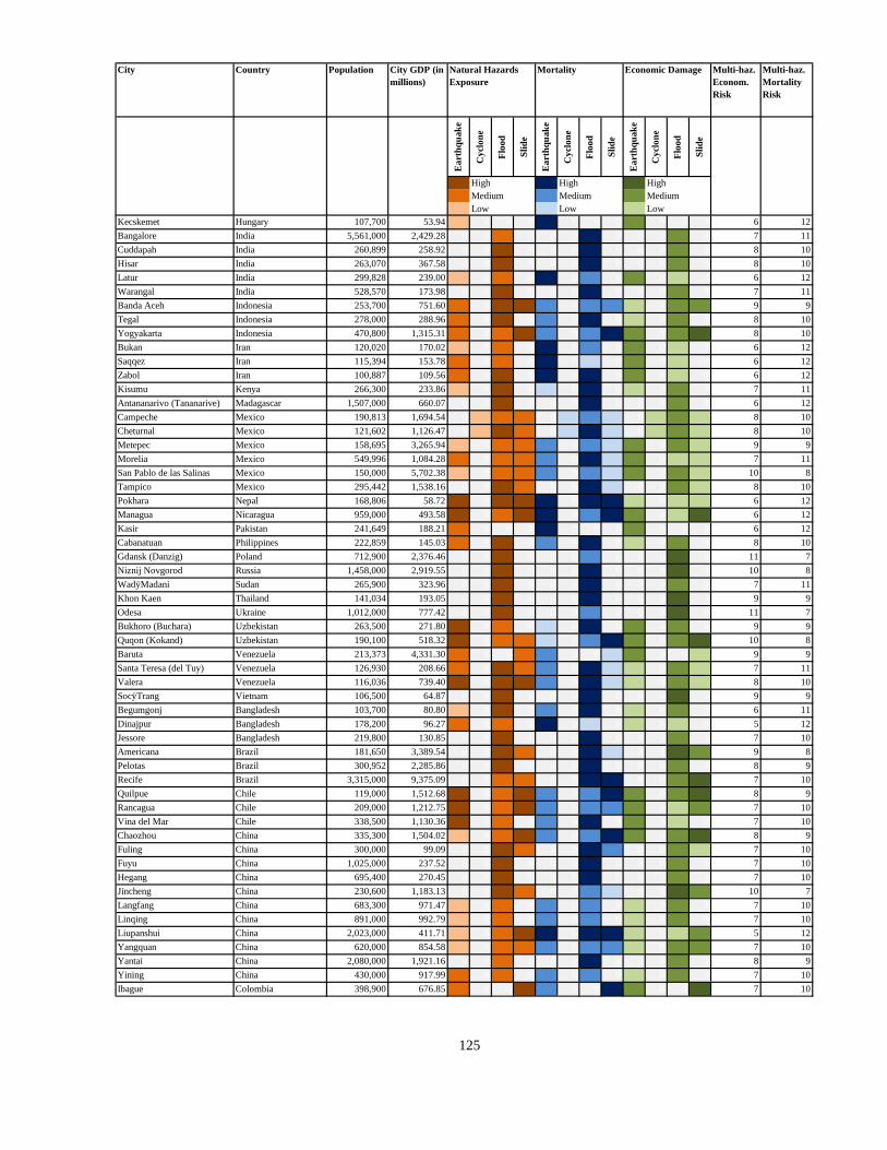
City Country Population City GDP (in
millions)
Multi-haz.
Econom.
Risk
Multi-haz.
Mortality
Risk
Ea
rth
qu
ak
e
Cy
clo
ne
Flo
od
Sli
de
Ea
rth
qu
ak
e
Cy
clo
ne
Flo
od
Sli
de
Ea
rth
qu
ak
e
Cy
clo
ne
Flo
od
Sli
de
3 High 3 High 3 High
2 Medium 2 Medium 2 Medium
1 Low 1 Low 1 Low
Natural Hazards
Exposure
Mortality Economic Damage
Kecskemet Hungary 107,700 53.94 1 0 0 0 3 0 0 0 2 0 0 0 6 12
Bangalore India 5,561,000 2,429.28 0 0 2 0 0 0 3 0 0 0 2 0 7 11
Cuddapah India 260,899 258.92 0 0 3 0 0 0 3 0 0 0 2 0 8 10
Hisar India 263,070 367.58 0 0 3 0 0 0 3 0 0 0 2 0 8 10
Latur India 299,828 239.00 1 0 2 0 3 0 2 0 2 0 1 0 6 12
Warangal India 528,570 173.98 0 0 3 0 0 0 3 0 0 0 2 0 7 11
Banda Aceh Indonesia 253,700 751.60 2 0 3 3 2 0 2 2 1 0 2 2 9 9
Tegal Indonesia 278,000 288.96 2 0 3 0 2 0 3 0 1 0 2 0 8 10
Yogyakarta Indonesia 470,800 1,315.31 2 0 2 3 2 0 2 3 2 0 2 3 8 10
Bukan Iran 120,020 170.02 1 0 2 0 3 0 2 0 2 0 1 0 6 12
Saqqez Iran 115,394 153.78 2 0 2 0 3 0 1 0 2 0 1 0 6 12
Zabol Iran 100,887 109.56 2 0 3 0 3 0 3 0 2 0 1 0 6 12
Kisumu Kenya 266,300 233.86 1 0 3 0 1 0 3 0 1 0 2 0 7 11
Antananarivo (Tananarive) Madagascar 1,507,000 660.07 0 0 3 0 0 0 3 0 0 0 2 0 6 12
Campeche Mexico 190,813 1,694.54 0 1 2 2 0 1 2 1 0 1 2 1 8 10
Cheturnal Mexico 121,602 1,126.47 0 1 3 2 0 1 3 1 0 1 2 1 8 10
Metepec Mexico 158,695 3,265.94 1 0 2 2 2 0 2 1 2 0 2 1 9 9
Morelia Mexico 549,996 1,084.28 2 0 2 2 2 0 3 1 2 0 1 1 7 11
San Pablo de las Salinas Mexico 150,000 5,702.38 1 0 2 2 2 0 2 1 2 0 2 1 10 8
Tampico Mexico 295,442 1,538.16 0 0 3 2 0 0 3 1 0 0 2 1 8 10
Pokhara Nepal 168,806 58.72 3 0 3 3 3 0 3 3 1 0 1 1 6 12
Managua Nicaragua 959,000 493.58 3 0 2 3 3 0 2 3 2 0 1 3 6 12
Kasir Pakistan 241,649 188.21 2 0 0 0 3 0 0 0 2 0 0 0 6 12
Cabanatuan Philippines 222,859 145.03 2 0 3 0 2 0 3 0 1 0 2 0 8 10
Gdansk (Danzig) Poland 712,900 2,376.46 0 0 3 0 0 0 2 0 0 0 3 0 11 7
Niznij Novgorod Russia 1,458,000 2,919.55 0 0 3 0 0 0 3 0 0 0 3 0 10 8
WadÿMadani Sudan 265,900 323.96 0 0 3 0 0 0 3 0 0 0 2 0 7 11
Khon Kaen Thailand 141,034 193.05 0 0 3 0 0 0 3 0 0 0 3 0 9 9
Odesa Ukraine 1,012,000 777.42 0 0 3 0 0 0 2 0 0 0 3 0 11 7
Bukhoro (Buchara) Uzbekistan 263,500 271.80 3 0 2 0 1 0 3 0 2 0 2 0 9 9
Quqon (Kokand) Uzbekistan 190,100 518.32 3 0 2 2 1 0 2 3 2 0 2 3 10 8
Baruta Venezuela 213,373 4,331.30 2 0 0 2 2 0 0 1 2 0 0 1 9 9
Santa Teresa (del Tuy) Venezuela 126,930 208.66 2 0 3 2 2 0 3 1 1 0 2 1 7 11
Valera Venezuela 116,036 739.40 3 0 3 3 2 0 3 1 1 0 2 1 8 10
SocÿTrang Vietnam 106,500 64.87 0 0 3 0 0 0 3 0 0 0 3 0 9 9
Begumgonj Bangladesh 103,700 80.80 1 0 3 0 2 0 3 0 1 0 2 0 6 11
Dinajpur Bangladesh 178,200 96.27 2 0 2 0 3 0 1 0 1 0 1 0 5 12
Jessore Bangladesh 219,800 130.85 0 0 3 0 0 0 3 0 0 0 2 0 7 10
Americana Brazil 181,650 3,389.54 0 0 3 2 0 0 3 1 0 0 3 2 9 8
Pelotas Brazil 300,952 2,285.86 0 0 3 0 0 0 3 0 0 0 2 0 8 9
Recife Brazil 3,315,000 9,375.09 0 0 2 2 0 0 3 3 0 0 2 3 7 10
Quilpue Chile 119,000 1,512.68 3 0 2 3 2 0 2 3 2 0 2 3 8 9
Rancagua Chile 209,000 1,212.75 3 0 2 3 2 0 2 2 2 0 1 2 7 10
Vina del Mar Chile 338,500 1,130.36 3 0 2 0 2 0 3 0 2 0 1 0 7 10
Chaozhou China 335,300 1,504.02 1 0 2 3 2 0 2 3 2 0 2 3 8 9
Fuling China 300,000 99.09 0 0 3 2 0 0 3 2 0 0 2 1 7 10
Fuyu China 1,025,000 237.52 0 0 3 0 0 0 3 0 0 0 2 0 7 10
Hegang China 695,400 270.45 0 0 3 0 0 0 3 0 0 0 2 0 7 10
Jincheng China 230,600 1,183.13 0 0 3 2 0 0 2 1 0 0 3 2 10 7
Langfang China 683,300 971.47 1 0 2 0 2 0 2 0 1 0 2 0 7 10
Linqing China 891,000 992.79 1 0 2 0 2 0 2 0 1 0 2 0 7 10
Liupanshui China 2,023,000 411.71 1 0 2 3 3 0 3 3 1 0 1 2 5 12
Yangquan China 620,000 854.58 1 0 2 2 2 0 2 2 1 0 2 2 7 10
Yantai China 2,080,000 1,921.16 0 0 2 0 0 0 3 0 0 0 2 0 8 9
Yining China 430,000 917.99 2 0 2 0 2 0 2 0 1 0 2 0 7 10
Ibague Colombia 398,900 676.85 2 0 0 3 2 0 0 3 2 0 0 3 7 10
125
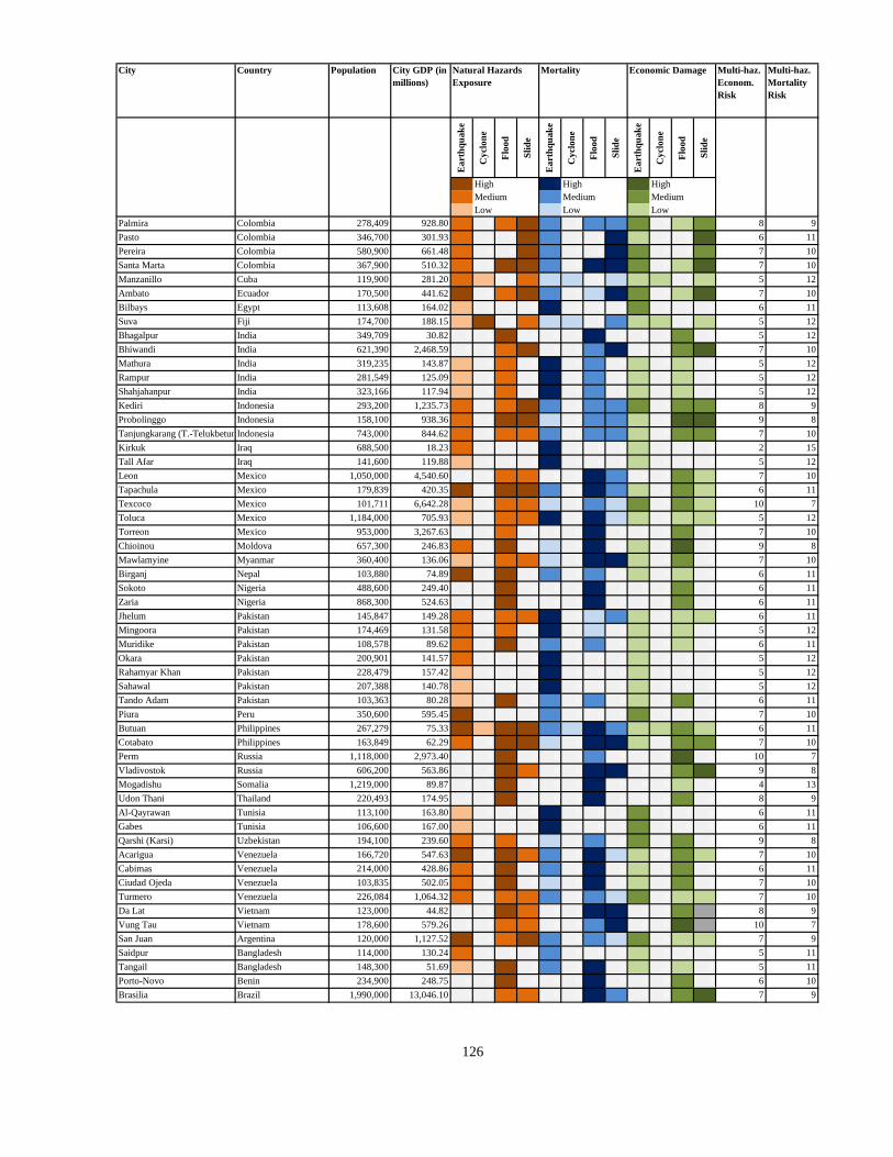
City Country Population City GDP (in
millions)
Multi-haz.
Econom.
Risk
Multi-haz.
Mortality
Risk
Ea
rth
qu
ak
e
Cy
clo
ne
Flo
od
Sli
de
Ea
rth
qu
ak
e
Cy
clo
ne
Flo
od
Sli
de
Ea
rth
qu
ak
e
Cy
clo
ne
Flo
od
Sli
de
3 High 3 High 3 High
2 Medium 2 Medium 2 Medium
1 Low 1 Low 1 Low
Natural Hazards
Exposure
Mortality Economic Damage
Palmira Colombia 278,409 928.80 2 0 2 3 2 0 2 2 2 0 1 2 8 9
Pasto Colombia 346,700 301.93 2 0 0 3 2 0 0 3 1 0 0 3 6 11
Pereira Colombia 580,900 661.48 2 0 0 3 2 0 0 3 2 0 0 2 7 10
Santa Marta Colombia 367,900 510.32 2 0 3 3 2 0 3 3 2 0 1 3 7 10
Manzanillo Cuba 119,900 281.20 2 1 0 2 1 1 0 1 1 1 0 1 5 12
Ambato Ecuador 170,500 441.62 3 0 2 3 2 0 1 3 2 0 1 3 7 10
Bilbays Egypt 113,608 164.02 1 0 0 0 3 0 0 0 2 0 0 0 6 11
Suva Fiji 174,700 188.15 1 3 0 2 1 1 0 2 1 1 0 1 5 12
Bhagalpur India 349,709 30.82 0 0 3 0 0 0 3 0 0 0 2 0 5 12
Bhiwandi India 621,390 2,468.59 0 0 2 3 0 0 2 3 0 0 2 3 7 10
Mathura India 319,235 143.87 1 0 2 0 3 0 2 0 1 0 1 0 5 12
Rampur India 281,549 125.09 1 0 2 0 3 0 2 0 1 0 1 0 5 12
Shahjahanpur India 323,166 117.94 1 0 2 0 3 0 2 0 1 0 1 0 5 12
Kediri Indonesia 293,200 1,235.73 2 0 2 3 2 0 2 2 2 0 2 2 8 9
Probolinggo Indonesia 158,100 938.36 2 0 3 3 1 0 2 2 1 0 3 3 9 8
Tanjungkarang (T.-Telukbetunk, Bandar LampunIndonesia 743,000 844.62 2 0 2 2 2 0 2 2 1 0 2 2 7 10
Kirkuk Iraq 688,500 18.23 2 0 0 0 3 0 0 0 1 0 0 0 2 15
Tall Afar Iraq 141,600 119.88 1 0 0 0 3 0 0 0 1 0 0 0 5 12
Leon Mexico 1,050,000 4,540.60 0 0 2 2 0 0 3 2 0 0 2 1 7 10
Tapachula Mexico 179,839 420.35 3 0 3 3 2 0 3 2 1 0 2 1 6 11
Texcoco Mexico 101,711 6,642.28 1 0 2 2 1 0 2 1 2 0 2 1 10 7
Toluca Mexico 1,184,000 705.93 1 0 2 2 3 0 3 1 1 0 1 1 5 12
Torreon Mexico 953,000 3,267.63 0 0 2 0 0 0 3 0 0 0 2 0 7 10
Chioinou Moldova 657,300 246.83 2 0 3 0 1 0 3 0 1 0 3 0 9 8
Mawlamyine Myanmar 360,400 136.06 1 0 2 2 1 0 3 3 1 0 2 0 7 10
Birganj Nepal 103,880 74.89 3 0 3 0 2 0 2 0 1 0 1 0 6 11
Sokoto Nigeria 488,600 249.40 0 0 3 0 0 0 3 0 0 0 2 0 6 11
Zaria Nigeria 868,300 524.63 0 0 3 0 0 0 3 0 0 0 2 0 6 11
Jhelum Pakistan 145,847 149.28 2 0 2 2 3 0 1 2 1 0 1 1 6 11
Mingoora Pakistan 174,469 131.58 2 0 2 0 3 0 1 0 1 0 1 0 5 12
Muridike Pakistan 108,578 89.62 2 0 3 0 2 0 2 0 1 0 1 0 6 11
Okara Pakistan 200,901 141.57 2 0 0 0 3 0 0 0 1 0 0 0 5 12
Rahamyar Khan Pakistan 228,479 157.42 1 0 0 0 3 0 0 0 1 0 0 0 5 12
Sahawal Pakistan 207,388 140.78 1 0 0 0 3 0 0 0 1 0 0 0 5 12
Tando Adam Pakistan 103,363 80.28 1 0 3 0 2 0 2 0 1 0 2 0 6 11
Piura Peru 350,600 595.45 3 0 0 0 2 0 0 0 2 0 0 0 7 10
Butuan Philippines 267,279 75.33 3 1 3 3 2 1 3 2 1 1 2 1 6 11
Cotabato Philippines 163,849 62.29 2 0 3 3 1 0 3 3 1 0 2 2 7 10
Perm Russia 1,118,000 2,973.40 0 0 3 0 0 0 2 0 0 0 3 0 10 7
Vladivostok Russia 606,200 563.86 0 0 3 2 0 0 3 3 0 0 2 3 9 8
Mogadishu Somalia 1,219,000 89.87 0 0 3 0 0 0 3 0 0 0 1 0 4 13
Udon Thani Thailand 220,493 174.95 0 0 3 0 0 0 3 0 0 0 2 0 8 9
Al-Qayrawan Tunisia 113,100 163.80 1 0 0 0 3 0 0 0 2 0 0 0 6 11
Gabes Tunisia 106,600 167.00 1 0 0 0 3 0 0 0 2 0 0 0 6 11
Qarshi (Karsi) Uzbekistan 194,100 239.60 2 0 2 0 1 0 2 0 2 0 2 0 9 8
Acarigua Venezuela 166,720 547.63 3 0 3 2 2 0 3 1 1 0 2 1 7 10
Cabimas Venezuela 214,000 428.86 2 0 3 0 2 0 3 0 1 0 2 0 6 11
Ciudad Ojeda Venezuela 103,835 502.05 2 0 3 0 1 0 3 0 1 0 2 0 7 10
Turmero Venezuela 226,084 1,064.32 2 0 2 2 2 0 2 1 2 0 1 1 7 10
Da Lat Vietnam 123,000 44.82 0 0 3 2 0 0 3 3 0 0 2 4 8 9
Vung Tau Vietnam 178,600 579.26 0 0 2 2 0 0 2 3 0 0 3 4 10 7
San Juan Argentina 120,000 1,127.52 3 0 2 3 2 0 2 1 2 0 1 1 7 9
Saidpur Bangladesh 114,000 130.24 2 0 0 0 2 0 0 0 1 0 0 0 5 11
Tangail Bangladesh 148,300 51.69 1 0 3 0 2 0 3 0 1 0 1 0 5 11
Porto-Novo Benin 234,900 248.75 0 0 3 0 0 0 3 0 0 0 2 0 6 10
Brasilia Brazil 1,990,000 13,046.10 0 0 2 2 0 0 3 2 0 0 2 3 7 9
126

City Country Population City GDP (in
millions)
Multi-haz.
Econom.
Risk
Multi-haz.
Mortality
Risk
Ea
rth
qu
ak
e
Cy
clo
ne
Flo
od
Sli
de
Ea
rth
qu
ak
e
Cy
clo
ne
Flo
od
Sli
de
Ea
rth
qu
ak
e
Cy
clo
ne
Flo
od
Sli
de
3 High 3 High 3 High
2 Medium 2 Medium 2 Medium
1 Low 1 Low 1 Low
Natural Hazards
Exposure
Mortality Economic Damage
Curitiba Brazil 2,525,000 12,465.23 0 0 2 0 0 0 3 0 0 0 2 0 7 9
Fortaleza Brazil 3,014,000 6,397.61 0 0 2 2 0 0 3 3 0 0 2 3 6 10
Santa Maria Brazil 230,464 1,680.27 0 0 3 2 0 0 3 2 0 0 2 2 7 9
Talcahuano Chile 277,000 694.87 3 0 2 0 2 0 2 0 1 0 1 0 6 10
Temuco Chile 260,000 642.35 3 0 2 3 2 0 2 3 1 0 1 1 6 10
Cangzhou China 440,400 954.57 1 0 2 0 2 0 2 0 1 0 2 0 7 9
Changzhi China 593,500 114.76 2 0 3 2 2 0 3 2 1 0 2 1 5 11
Changzhou China 886,000 4,501.09 0 0 2 0 0 0 2 0 0 0 3 0 10 6
Foshan China 468,400 6,261.63 0 0 2 3 0 0 2 3 0 0 3 3 10 6
Fushun China 1,411,300 2,469.52 0 0 2 0 0 0 3 0 0 0 2 0 8 8
Guiyang China 2,533,000 982.21 0 0 2 2 0 0 3 3 0 0 2 2 6 10
Nanyang China 1,613,700 1,389.06 0 0 2 2 0 0 3 3 0 0 2 2 7 9
Panzhihua China 635,500 471.30 2 0 2 3 2 0 2 3 1 0 1 2 6 10
Suzhou China 1,183,000 3,973.22 0 0 2 2 0 0 2 2 0 0 3 2 9 7
Wuxi China 1,127,000 2,806.50 0 0 2 0 0 0 2 0 0 0 2 0 9 7
Xiamen China 1,265,900 338.00 0 1 2 0 0 1 2 0 0 1 1 0 4 12
Yinchuan China 586,000 586.26 3 0 2 0 2 0 2 0 1 0 2 0 6 10
Armenia Colombia 294,300 669.98 2 0 0 3 2 0 0 2 2 0 0 2 7 9
Barrancabermeja Colombia 183,300 314.03 2 0 3 2 2 0 3 1 1 0 1 1 6 10
Buenaventura Colombia 324,207 423.40 2 0 2 3 2 0 2 2 2 0 1 2 6 10
Neiva Colombia 312,300 434.75 3 0 2 3 2 0 2 3 2 0 1 3 6 10
Holguin Cuba 305,000 636.95 2 0 0 2 2 0 0 1 2 0 0 2 7 9
La Vega Dominican Republic 106,200 667.86 3 0 3 3 1 0 2 2 2 0 2 3 8 8
Cuenca Ecuador 271,400 812.65 2 0 2 3 2 0 2 3 2 0 1 3 7 9
Alappuzha (Alleppey) India 177,079 271.70 0 0 3 2 0 0 3 3 0 0 2 2 7 9
Jaipur India 2,145,000 1,318.87 0 0 2 0 0 0 3 0 0 0 2 0 6 10
Kollam (Quilon) India 379,975 589.40 0 0 3 2 0 0 3 3 0 0 2 2 7 9
Nagpur India 2,062,000 2,193.80 0 0 2 0 0 0 3 0 0 0 2 0 7 9
Cilacap Indonesia 254,900 271.23 2 0 3 0 2 0 2 0 1 0 2 0 7 9
Pasuruan Indonesia 160,600 547.42 2 0 3 3 1 0 2 2 1 0 2 2 8 8
Taman (Jawa Tengah) Indonesia 102,800 462.88 2 0 3 3 1 0 2 2 1 0 2 2 9 7
Aguascalientes Mexico 594,092 3,329.57 0 0 2 2 0 0 3 1 0 0 2 1 7 9
Boca del Rio Mexico 123,891 578.67 1 0 3 0 1 0 3 0 1 0 2 0 6 10
Colima Mexico 119,639 920.14 3 0 2 3 2 0 2 2 2 0 1 2 7 9
Huixquilucan Mexico 107,951 9,817.37 1 0 0 2 1 0 0 1 3 0 0 1 10 6
Merida Mexico 662,530 2,590.20 0 0 2 0 0 0 3 0 0 0 2 0 6 10
Nuevo Laredo Mexico 308,828 8,864.70 0 0 2 0 0 0 3 0 0 0 3 0 9 7
Poza Rica de Hidalgo Mexico 151,441 1,244.91 1 0 2 3 2 0 2 1 1 0 2 1 7 9
Puerto Vallarta Mexico 151,432 536.29 3 1 2 3 2 1 2 1 1 1 1 1 6 10
Queretaro Mexico 536,463 3,377.44 0 0 2 2 0 0 3 1 0 0 2 1 7 9
San Luis Rio Colorado Mexico 126,645 1,093.79 3 0 2 0 2 0 2 0 2 0 1 0 7 9
Veracruz Mexico 411,582 1,381.21 1 0 0 2 2 0 0 1 2 0 0 1 6 10
Mohammedia Morocco 188,619 1,526.15 0 0 3 0 0 0 3 0 0 0 2 0 8 8
Daska Pakistan 101,500 86.84 2 0 3 0 2 0 2 0 1 0 1 0 5 11
Jacobabad Pakistan 137,733 91.82 2 0 2 0 3 0 1 0 1 0 1 0 5 11
Khairpur Pakistan 102,188 132.75 2 0 0 0 2 0 0 0 1 0 0 0 5 11
Kohat Pakistan 125,271 94.88 2 0 2 0 2 0 1 0 1 0 1 0 5 11
Nawabshah Pakistan 183,110 132.36 1 0 0 0 3 0 0 0 1 0 0 0 5 11
Sadiqabad Pakistan 141,509 117.97 1 0 2 0 2 0 1 0 1 0 1 0 5 11
Shikarpur Pakistan 133,259 97.55 2 0 2 0 3 0 1 0 1 0 1 0 5 11
Huancayo Peru 282,400 765.31 2 0 2 3 2 0 2 2 2 0 1 3 7 9
Naga Philippines 137,810 148.97 3 0 3 3 1 0 3 2 1 0 2 2 7 9
Olongapo Philippines 194,260 63.07 3 0 3 3 2 0 3 3 1 0 2 2 6 10
Stettin Poland 416,600 1,502.76 0 0 3 0 0 0 2 0 0 0 3 0 10 6
Chabarovsk Russia 614,000 535.37 0 0 3 2 0 0 2 3 0 0 2 3 8 8
Chimki Russia 133,500 10,212.53 0 0 3 0 0 0 1 0 0 0 3 0 13 3
127
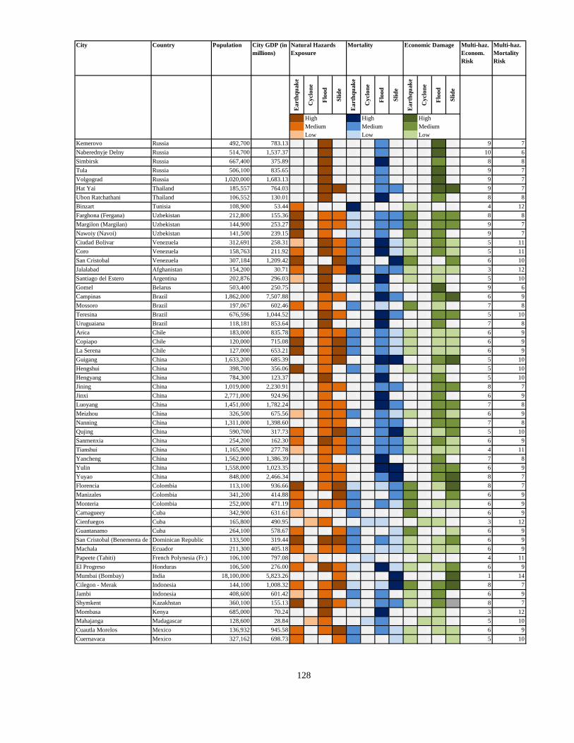
City Country Population City GDP (in
millions)
Multi-haz.
Econom.
Risk
Multi-haz.
Mortality
Risk
Ea
rth
qu
ak
e
Cy
clo
ne
Flo
od
Sli
de
Ea
rth
qu
ak
e
Cy
clo
ne
Flo
od
Sli
de
Ea
rth
qu
ak
e
Cy
clo
ne
Flo
od
Sli
de
3 High 3 High 3 High
2 Medium 2 Medium 2 Medium
1 Low 1 Low 1 Low
Natural Hazards
Exposure
Mortality Economic Damage
Kemerovo Russia 492,700 783.13 0 0 3 0 0 0 2 0 0 0 3 0 9 7
Naberednyje Delny Russia 514,700 1,537.37 0 0 3 0 0 0 2 0 0 0 3 0 10 6
Simbirsk Russia 667,400 375.89 0 0 3 0 0 0 3 0 0 0 2 0 8 8
Tula Russia 506,100 835.65 0 0 3 0 0 0 2 0 0 0 3 0 9 7
Volgograd Russia 1,020,000 1,683.13 0 0 3 0 0 0 2 0 0 0 3 0 9 7
Hat Yai Thailand 185,557 764.03 0 0 3 3 0 0 2 2 0 0 3 3 9 7
Ubon Ratchathani Thailand 106,552 130.01 0 0 3 0 0 0 3 0 0 0 2 0 8 8
Binzart Tunisia 108,900 53.44 2 0 0 0 3 0 0 0 1 0 0 0 4 12
Farghona (Fergana) Uzbekistan 212,800 155.36 3 0 2 2 1 0 2 2 2 0 2 2 8 8
Margilon (Margilan) Uzbekistan 144,900 253.27 3 0 2 2 1 0 2 2 2 0 2 2 9 7
Nawoiy (Navoi) Uzbekistan 141,500 239.15 3 0 2 0 1 0 2 0 2 0 2 0 9 7
Ciudad Bolivar Venezuela 312,691 258.31 1 0 3 2 2 0 3 1 1 0 2 1 5 11
Coro Venezuela 158,763 211.92 2 0 3 2 2 0 3 1 1 0 2 1 5 11
San Cristobal Venezuela 307,184 1,209.42 3 0 0 3 2 0 0 3 2 0 0 2 6 10
Jalalabad Afghanistan 154,200 30.71 2 0 3 2 3 0 2 2 1 0 1 1 3 12
Santiago del Estero Argentina 202,876 296.03 1 0 3 0 2 0 3 0 1 0 1 0 5 10
Gomel Belarus 503,400 250.75 0 0 3 0 0 0 2 0 0 0 3 0 9 6
Campinas Brazil 1,862,000 7,507.88 0 0 2 2 0 0 3 2 0 0 2 3 6 9
Mossoro Brazil 197,067 602.46 2 0 2 0 2 0 1 0 2 0 1 0 7 8
Teresina Brazil 676,596 1,044.52 0 0 3 2 0 0 3 2 0 0 2 2 5 10
Uruguaiana Brazil 118,181 853.64 0 0 3 0 0 0 3 0 0 0 2 0 7 8
Arica Chile 183,000 835.78 2 0 2 2 2 0 2 1 1 0 1 1 6 9
Copiapo Chile 120,000 715.08 3 0 2 3 2 0 2 1 1 0 1 1 6 9
La Serena Chile 127,000 653.21 3 0 2 3 2 0 2 1 1 0 1 1 6 9
Guigang China 1,633,200 685.39 0 0 2 3 0 0 3 3 0 0 2 3 5 10
Hengshui China 398,700 356.06 3 0 2 0 2 0 2 0 1 0 1 0 5 10
Hengyang China 784,300 123.37 0 0 3 0 0 0 3 0 0 0 2 0 5 10
Jining China 1,019,000 2,230.91 0 0 2 2 0 0 2 2 0 0 2 2 8 7
Jinxi China 2,771,000 924.96 0 0 2 0 0 0 3 0 0 0 2 0 6 9
Luoyang China 1,451,000 1,782.24 0 0 2 2 0 0 3 2 0 0 2 2 7 8
Meizhou China 326,500 675.56 1 0 2 2 2 0 2 1 1 0 2 1 6 9
Nanning China 1,311,000 1,398.60 0 0 2 2 0 0 2 2 0 0 2 2 7 8
Qujing China 590,700 317.73 2 0 2 3 2 0 2 3 1 0 1 2 5 10
Sanmenxia China 254,200 162.30 2 0 3 2 2 0 2 2 1 0 2 1 6 9
Tianshui China 1,165,900 277.78 1 0 2 2 2 0 2 2 1 0 1 1 4 11
Yancheng China 1,562,000 1,386.39 0 0 2 0 0 0 3 0 0 0 2 0 7 8
Yulin China 1,558,000 1,023.35 0 0 2 2 0 0 3 3 0 0 2 2 6 9
Yuyao China 848,000 2,466.34 0 0 2 2 0 0 2 3 0 0 2 3 8 7
Florencia Colombia 113,100 936.66 3 0 2 3 1 0 1 2 2 0 1 3 8 7
Manizales Colombia 341,200 414.88 2 0 0 3 2 0 0 2 2 0 0 2 6 9
Monteria Colombia 252,000 471.19 2 0 2 2 2 0 2 1 2 0 1 1 6 9
Camagueey Cuba 342,900 631.61 1 0 0 0 2 0 0 0 2 0 0 0 6 9
Cienfuegos Cuba 165,800 490.95 0 1 2 0 0 1 1 0 0 1 1 0 3 12
Guantanamo Cuba 264,100 578.67 2 0 0 2 2 0 0 1 2 0 0 1 6 9
San Cristobal (Benementa de San Cristobal)Dominican Republic 133,500 319.44 3 0 3 3 2 0 2 1 1 0 1 2 6 9
Machala Ecuador 211,300 405.18 2 0 2 2 2 0 1 1 1 0 1 1 6 9
Papeete (Tahiti) French Polynesia (Fr.) 106,100 797.08 0 1 0 0 0 1 0 0 0 1 0 0 4 11
El Progreso Honduras 106,500 276.00 2 0 3 2 1 0 3 1 1 0 1 2 6 9
Mumbai (Bombay) India 18,100,000 5,823.26 0 0 0 2 0 0 0 3 0 0 0 3 1 14
Cilegon - Merak Indonesia 144,100 1,008.32 2 0 2 3 1 0 1 3 2 0 2 3 8 7
Jambi Indonesia 408,600 601.42 1 0 2 0 2 0 2 0 1 0 2 0 6 9
Shymkent Kazakhstan 360,100 155.13 3 0 3 2 1 0 2 2 1 0 2 4 8 7
Mombasa Kenya 685,000 70.24 0 0 3 0 0 0 3 0 0 0 1 0 3 12
Mahajanga Madagascar 128,600 28.84 0 1 2 0 0 1 2 0 0 1 1 0 5 10
Cuautla Morelos Mexico 136,932 945.58 2 0 2 3 2 0 2 1 1 0 1 1 6 9
Cuernavaca Mexico 327,162 698.73 2 0 0 2 2 0 0 1 1 0 0 1 5 10
128

City Country Population City GDP (in
millions)
Multi-haz.
Econom.
Risk
Multi-haz.
Mortality
Risk
Ea
rth
qu
ak
e
Cy
clo
ne
Flo
od
Sli
de
Ea
rth
qu
ak
e
Cy
clo
ne
Flo
od
Sli
de
Ea
rth
qu
ak
e
Cy
clo
ne
Flo
od
Sli
de
3 High 3 High 3 High
2 Medium 2 Medium 2 Medium
1 Low 1 Low 1 Low
Natural Hazards
Exposure
Mortality Economic Damage
Saltillo Mexico 562,587 2,295.52 0 0 2 2 0 0 3 1 0 0 2 1 6 9
Tehuacan Mexico 204,598 858.70 1 0 2 3 2 0 2 1 1 0 1 1 6 9
Tepic Mexico 265,817 727.20 3 0 0 3 2 0 0 3 1 0 0 2 5 10
Xalapa Mexico 373,076 823.09 1 0 0 3 2 0 0 3 1 0 0 2 5 10
Safi Morocco 103,100 77.23 1 0 0 0 3 0 0 0 1 0 0 0 4 11
Tanger Morocco 578,800 529.80 0 0 3 2 0 0 3 2 0 0 2 4 5 10
Maputo Mozambique 3,025,000 744.08 0 0 2 2 0 0 3 3 0 0 1 0 4 11
Niamey Niger 182,450 215.48 0 0 3 0 0 0 3 0 0 0 2 0 5 10
Katsina Nigeria 377,400 219.81 0 0 3 0 0 0 3 0 0 0 2 0 5 10
Abbottabad Pakistan 105,999 82.76 2 0 0 3 2 0 0 3 1 0 0 2 4 11
Bahawalnagar Pakistan 109,642 96.75 2 0 0 0 2 0 0 0 1 0 0 0 4 11
Barewala Pakistan 149,857 104.16 1 0 0 0 2 0 0 0 1 0 0 0 4 11
Gojra Pakistan 114,967 80.86 1 0 0 0 2 0 0 0 1 0 0 0 4 11
Hafizabad Pakistan 130,216 90.19 2 0 0 0 3 0 0 0 1 0 0 0 4 11
Jaranwala Pakistan 103,308 73.06 2 0 2 0 2 0 1 0 1 0 1 0 4 11
Khanewal Pakistan 132,962 91.53 1 0 0 0 2 0 0 0 1 0 0 0 4 11
Pakpattan Pakistan 107,791 79.10 1 0 0 0 2 0 0 0 1 0 0 0 4 11
Cusco Peru 279,600 412.23 2 0 0 3 2 0 0 2 1 0 0 2 6 9
Iquitos Peru 340,200 489.49 1 0 2 0 2 0 2 0 1 0 1 0 6 9
Cagayan de Oro Philippines 461,877 292.67 2 0 2 3 2 0 2 3 1 0 1 3 5 10
Cebu Philippines 718,821 719.16 2 0 0 3 2 0 0 3 1 0 0 2 5 10
Legazpi Philippines 157,010 97.57 3 0 3 3 1 0 2 2 1 0 2 1 6 9
San Pablo Philippines 207,927 76.79 3 0 3 3 2 0 3 2 1 0 2 1 5 10
Tarlac Philippines 262,481 41.16 2 0 3 0 2 0 3 0 1 0 2 0 5 10
Bydgoszcz Poland 386,300 830.56 0 0 3 0 0 0 2 0 0 0 3 0 9 6
Wroclaw Poland 636,800 1,225.04 0 0 3 0 0 0 2 0 0 0 3 0 9 6
Lyubercy Russia 163,900 7,259.96 0 0 3 0 0 0 1 0 0 0 3 0 12 3
Odincovo Russia 127,400 8,505.17 0 0 3 0 0 0 1 0 0 0 3 0 12 3
Morogoro Tanzania 235,200 149.88 1 0 3 2 1 0 3 2 1 0 1 4 5 10
Tabora Tanzania 1,703,000 121.13 0 0 3 0 0 0 3 0 0 0 1 0 3 12
Rayong Thailand 106,585 2,397.71 0 0 3 0 0 0 2 0 0 0 3 0 11 4
Puerto la Cruz Venezuela 205,635 625.19 2 0 2 3 2 0 2 1 1 0 1 1 5 10
Asadabad Afghanistan 101,600 30.41 2 0 2 2 2 0 1 2 1 0 1 1 3 11
Herat Afghanistan 161,700 61.72 2 0 0 0 3 0 0 0 1 0 0 0 3 11
Mehtar Lam Afghanistan 118,500 30.50 2 0 2 2 2 0 1 2 1 0 1 1 3 11
Quandahar Afghanistan 329,300 4.22 2 0 0 0 3 0 0 0 1 0 0 0 1 13
Qunduz Afghanistan 111,200 32.06 3 0 2 0 3 0 1 0 1 0 1 0 3 11
Luanda Angola 2,571,600 1,482.51 0 0 2 0 0 0 3 0 0 0 1 0 3 11
Salta Argentina 457,223 427.19 2 0 0 3 2 0 0 1 1 0 0 1 4 10
San Salvador de Jujuy Argentina 226,961 335.57 2 0 2 0 2 0 2 0 1 0 1 0 4 10
Noakhali Bangladesh 103,700 112.08 1 0 0 0 2 0 0 0 1 0 0 0 4 10
Satkhira Bangladesh 100,800 60.26 0 0 3 0 0 0 3 0 0 0 2 0 5 9
Bujumbura Burundi 315,000 38.93 1 0 3 2 1 0 3 2 1 0 1 0 3 11
Garoua Cameroon 313,000 203.26 0 0 3 0 0 0 3 0 0 0 1 0 3 11
Calama Chile 124,000 953.02 2 0 2 2 2 0 2 1 1 0 1 1 6 8
Chillan Chile 167,000 530.90 2 0 2 0 2 0 2 0 1 0 1 0 5 9
Iquique Chile 170,000 820.04 3 0 0 2 2 0 0 1 1 0 0 1 5 9
Talca Chile 179,000 626.49 2 0 2 3 2 0 2 1 1 0 1 1 5 9
Valparaiso Chile 285,000 444.72 3 0 0 2 2 0 0 1 1 0 0 1 4 10
Baoding China 701,500 1,901.74 0 0 2 0 0 0 2 0 0 0 2 0 8 6
Benxi China 957,000 1,377.60 0 0 2 0 0 0 2 0 0 0 2 0 7 7
Changde China 1,374,000 998.26 0 0 2 2 0 0 3 3 0 0 2 2 6 8
Chifeng China 1,087,000 1,372.56 0 0 2 0 0 0 2 0 0 0 2 0 7 7
Dandong China 700,200 1,891.79 0 0 2 0 0 0 2 0 0 0 2 0 8 6
Huainan China 1,349,100 1,003.02 0 0 2 2 0 0 2 2 0 0 2 2 6 8
Huzhou China 1,077,000 1,543.86 0 0 2 2 0 0 2 3 0 0 2 2 7 7
129

City Country Population City GDP (in
millions)
Multi-haz.
Econom.
Risk
Multi-haz.
Mortality
Risk
Ea
rth
qu
ak
e
Cy
clo
ne
Flo
od
Sli
de
Ea
rth
qu
ak
e
Cy
clo
ne
Flo
od
Sli
de
Ea
rth
qu
ak
e
Cy
clo
ne
Flo
od
Sli
de
3 High 3 High 3 High
2 Medium 2 Medium 2 Medium
1 Low 1 Low 1 Low
Natural Hazards
Exposure
Mortality Economic Damage
Jiangmen China 427,900 1,761.45 0 0 2 3 0 0 2 3 0 0 2 3 8 6
Jiaxing China 791,000 2,077.39 0 0 2 0 0 0 2 0 0 0 2 0 8 6
Liuzhou China 928,000 1,528.26 0 0 2 2 0 0 2 3 0 0 2 2 7 7
Sucheng China 237,000 512.25 1 0 2 0 1 0 1 0 1 0 2 0 6 8
Suining China 1,428,000 914.02 0 0 2 0 0 0 3 0 0 0 2 0 6 8
Taicheng China 950,000 1,446.51 0 0 2 2 0 0 2 3 0 0 2 2 7 7
Tangshan China 1,671,000 67.95 3 0 0 0 3 0 0 0 1 0 0 0 2 12
Cucuta Colombia 723,200 129.21 2 0 2 2 2 0 2 2 1 0 1 1 3 11
Valledupar Colombia 274,300 292.80 2 0 2 2 2 0 2 2 1 0 1 2 5 9
Villavicencio Colombia 284,600 266.18 2 0 2 3 2 0 2 3 1 0 1 2 5 9
Matanzas Cuba 140,200 299.29 0 1 0 0 0 1 0 0 0 1 0 0 2 12
Praha (Prague, Prag) Czech Republic 1,226,000 10,593.07 0 0 2 0 0 0 2 0 0 0 3 0 10 4
Eloy Alfaro (Alfaro) Ecuador 137,800 792.34 2 0 2 3 1 0 1 2 2 0 1 3 7 7
Ibarra Ecuador 122,200 193.03 3 0 2 3 1 0 1 3 1 0 1 3 5 9
San Miguel El Salvador 227,414 343.40 2 0 2 3 2 0 1 2 1 0 1 2 5 9
Accra Ghana 1,976,000 1,031.18 0 0 2 0 0 0 3 0 0 0 2 0 4 10
Bilaspur India 330,291 190.96 0 0 3 0 0 0 3 0 0 0 2 0 5 9
Coimbatore India 1,292,000 784.19 0 0 2 2 0 0 3 3 0 0 2 2 5 9
Indore India 1,428,000 896.10 0 0 2 2 0 0 3 3 0 0 2 2 5 9
Korba India 315,695 75.02 0 0 3 0 0 0 3 0 0 0 1 0 4 10
Nashik (Nasik) India 1,136,000 978.54 0 0 2 2 0 0 3 3 0 0 2 2 5 9
Pemalang Indonesia 109,300 171.38 2 0 3 0 1 0 2 0 1 0 2 0 7 7
Masjed-e Soleyman Iran 116,883 16.02 3 0 0 0 3 0 0 0 1 0 0 0 2 12
Cordoba Mexico 133,807 1,116.13 1 0 2 3 1 0 2 2 1 0 1 2 6 8
Matamoros Mexico 376,279 2,456.22 0 0 2 0 0 0 3 0 0 0 2 0 6 8
Orizaba Mexico 118,552 1,093.84 1 0 2 3 1 0 2 3 1 0 1 2 6 8
Santa Catarina Mexico 225,976 3,879.31 0 0 2 3 0 0 2 2 0 0 2 2 7 7
Tultilan (Buenavista) Mexico 190,000 1,510.80 1 0 0 0 2 0 0 0 2 0 0 0 6 8
Uruapan Mexico 225,816 585.54 3 0 0 3 2 0 0 2 1 0 0 1 5 9
Taunggyi Myanmar 154,100 59.96 3 0 2 3 1 0 2 3 1 0 2 0 5 9
Jimeta Nigeria 213,300 125.73 0 0 3 0 0 0 3 0 0 0 1 0 4 10
Mubi Nigeria 194,000 101.94 0 0 3 0 0 0 3 0 0 0 1 0 4 10
Chishtian Mandi Pakistan 101,659 81.59 1 0 0 0 2 0 0 0 1 0 0 0 4 10
Ica Peru 183,700 416.87 3 0 0 2 2 0 0 1 2 0 0 1 6 8
Sullana Peru 180,400 410.31 3 0 2 0 2 0 1 0 2 0 1 0 6 8
Antipolo Philippines 470,866 155.75 3 0 0 3 2 0 0 3 1 0 0 3 3 11
General Santos Philippines 411,822 290.59 2 0 2 2 2 0 2 2 1 0 1 1 5 9
Iloilo Philippines 365,820 654.58 2 0 0 0 2 0 0 0 1 0 0 0 5 9
San Jose Philippines 108,254 53.30 2 0 3 3 1 0 3 3 1 0 2 2 5 9
Urdaneta Philippines 111,582 42.99 2 0 3 0 1 0 2 0 1 0 2 0 5 9
Astrachan Russia 486,100 934.76 0 0 3 0 0 0 2 0 0 0 2 0 8 6
Krasnojarsk Russia 977,000 2,551.57 0 0 2 2 0 0 2 3 0 0 2 3 8 6
Mytisci Russia 155,700 2,851.53 0 0 3 0 0 0 1 0 0 0 3 0 11 3
Saratov Russia 915,000 1,177.52 0 0 3 0 0 0 2 0 0 0 2 0 8 6
Tomsk Russia 482,100 1,767.23 0 0 3 0 0 0 2 0 0 0 3 0 9 5
Saint-Louis Senegal 144,100 82.10 0 0 3 0 0 0 3 0 0 0 1 0 4 10
Novi Sad Serbia and Monten. 182,778 113.91 1 0 3 0 1 0 2 0 1 0 2 0 9 5
Kassala Sudan 295,100 307.76 0 0 3 0 0 0 3 0 0 0 2 0 5 9
Kusti Sudan 218,400 73.48 0 0 3 0 0 0 3 0 0 0 1 0 4 10
Musoma Tanzania 131,500 88.94 1 0 3 0 1 0 3 0 1 0 1 0 4 10
Barinas Venezuela 228,598 305.22 2 0 2 3 2 0 2 2 1 0 1 1 4 10
Cumana Venezuela 269,428 305.28 3 0 2 2 2 0 2 1 1 0 1 1 4 10
Guacara Venezuela 137,816 574.76 2 0 2 2 2 0 2 1 1 0 1 1 5 9
Los Teques Venezuela 183,142 1,365.65 2 0 0 2 2 0 0 1 2 0 0 1 6 8
Maracay Venezuela 1,100,000 216.07 2 0 0 2 3 0 0 2 1 0 0 1 2 12
Maturin Venezuela 283,318 379.80 2 0 2 2 2 0 2 1 1 0 1 1 4 10
130

City Country Population City GDP (in
millions)
Multi-haz.
Econom.
Risk
Multi-haz.
Mortality
Risk
Ea
rth
qu
ak
e
Cy
clo
ne
Flo
od
Sli
de
Ea
rth
qu
ak
e
Cy
clo
ne
Flo
od
Sli
de
Ea
rth
qu
ak
e
Cy
clo
ne
Flo
od
Sli
de
3 High 3 High 3 High
2 Medium 2 Medium 2 Medium
1 Low 1 Low 1 Low
Natural Hazards
Exposure
Mortality Economic Damage
Merida Venezuela 230,101 366.72 3 0 2 3 2 0 2 1 1 0 1 1 4 10
Qaleh-ye Naw Afghanistan 115,200 17.44 2 0 0 0 2 0 0 0 1 0 0 0 2 11
Neuquen Argentina 327,374 1,730.86 0 0 2 0 0 0 3 0 0 0 2 0 5 8
Oruro Bolivia 232,311 192.69 2 0 3 0 2 0 2 0 1 0 1 0 4 9
Foz do Iguacu Brazil 256,349 1,663.14 0 0 3 2 0 0 2 1 0 0 2 2 6 7
Osorno Chile 129,000 451.84 2 0 2 3 2 0 2 1 1 0 1 1 5 8
Valdivia Chile 124,000 498.78 2 0 2 2 2 0 2 1 1 0 1 1 5 8
Baiyin China 445,200 262.05 3 0 0 0 2 0 0 0 1 0 0 0 3 10
Fuxin China 785,000 1,544.34 0 0 2 2 0 0 2 2 0 0 2 2 7 6
Fuyang China 1,729,500 573.40 0 0 2 0 0 0 3 0 0 0 2 0 5 8
Guilin China 611,200 1,038.19 0 0 2 3 0 0 2 3 0 0 2 3 6 7
Huaiyin China 521,800 2,376.73 0 0 2 0 0 0 2 0 0 0 2 0 8 5
Jinzhou China 834,000 1,516.09 0 0 2 2 0 0 2 2 0 0 2 2 7 6
Mianyang China 1,065,000 869.48 0 0 2 2 0 0 2 2 0 0 2 2 6 7
Pingdingshan China 723,000 1,340.23 0 0 2 2 0 0 2 3 0 0 2 2 7 6
Pingxiang China 1,502,000 542.37 0 0 2 2 0 0 3 3 0 0 2 2 5 8
Shaoxing China 324,300 3,637.83 0 0 2 2 0 0 2 1 0 0 3 2 9 4
Songyuan China 502,100 88.09 0 0 3 0 0 0 3 0 0 0 1 0 4 9
Taizhou China 588,000 1,947.96 0 0 2 0 0 0 2 0 0 0 2 0 8 5
Wuhai China 391,000 238.87 2 0 2 2 2 0 2 1 1 0 1 1 4 9
Yanan China 332,000 132.85 0 0 3 0 0 0 3 0 0 0 2 0 5 8
Sincelejo Colombia 231,500 377.44 2 0 0 2 2 0 0 1 1 0 0 1 5 8
Sogamoso Colombia 111,800 412.01 2 0 2 3 1 0 1 2 1 0 1 2 6 7
Tulua Colombia 157,300 266.10 2 0 2 3 2 0 1 1 1 0 1 2 5 8
Bayamo Cuba 181,900 372.97 2 0 0 0 2 0 0 0 1 0 0 0 5 8
Esmeraldas Ecuador 129,900 224.76 3 0 2 3 2 0 1 2 1 0 1 2 5 8
Riobamba Ecuador 125,100 269.54 3 0 2 3 1 0 1 2 1 0 1 2 5 8
Bhopal India 1,576,000 659.67 0 0 2 0 0 0 3 0 0 0 1 0 4 9
Jamshedpur India 1,002,000 659.80 0 0 2 2 0 0 2 3 0 0 1 1 4 9
Kozhikode (Calicut) India 1,115,000 596.85 0 0 2 2 0 0 3 3 0 0 1 1 4 9
Madurai India 1,275,000 1,105.93 0 0 2 0 0 0 3 0 0 0 2 0 5 8
Manado Indonesia 344,100 462.89 2 0 0 3 2 0 0 3 1 0 0 2 4 9
Tasikmalaya Indonesia 221,500 886.55 2 0 0 3 2 0 0 2 1 0 0 2 5 8
Nakuru Kenya 319,200 224.70 1 0 2 2 1 0 2 2 1 0 1 4 4 9
Blantyre Malawi 518,800 287.40 1 0 0 2 2 0 0 3 1 0 0 4 4 9
Kota Baharu Malaysia 233,673 2,110.38 0 0 3 0 0 0 3 0 0 0 2 0 5 8
Sungai Petani Malaysia 170,000 1,377.01 0 0 3 2 0 0 3 2 0 0 2 4 5 8
Chilpancingo Mexico 142,746 476.82 3 0 0 3 2 0 0 2 1 0 0 1 4 9
Ciudad del Carmen Mexico 126,024 183.53 0 0 3 0 0 0 3 0 0 0 1 0 4 9
Ciudad Valles Mexico 105,721 427.53 0 0 3 3 0 0 3 1 0 0 2 1 5 8
Durango Mexico 427,135 1,352.39 0 0 2 0 0 0 3 0 0 0 2 0 5 8
Ensenada Mexico 223,492 1,158.09 1 0 0 0 2 0 0 0 1 0 0 0 5 8
Pachuca Mexico 231,602 643.39 1 0 0 3 2 0 0 2 1 0 0 1 4 9
Mergui Myanmar 143,700 52.03 0 0 2 2 0 0 2 3 0 0 2 0 5 8
Masaya Nicaragua 110,000 327.62 3 0 2 3 1 0 1 2 1 0 1 2 6 7
Maradi Niger 503,061 39.60 0 0 3 0 0 0 3 0 0 0 1 0 2 11
Muzaffargarh Pakistan 121,641 5.32 2 0 2 3 2 0 1 3 1 0 1 1 1 12
Pucallpa Peru 227,500 335.30 1 0 2 0 2 0 1 0 1 0 1 0 5 8
Bacolod Philippines 429,076 564.68 2 0 0 2 2 0 0 2 1 0 0 2 4 9
San Carlos (Pangasinan) Philippines 154,264 41.19 2 0 3 0 1 0 3 0 1 0 1 0 4 9
Surigao Philippines 118,534 40.45 3 2 0 3 1 1 0 3 1 1 0 2 2 11
Plock Poland 130,900 525.17 0 0 3 0 0 0 2 0 0 0 3 0 9 4
Jaroslavl Russia 616,700 1,160.67 0 0 3 0 0 0 2 0 0 0 2 0 8 5
Maribor Slovenia 100,900 1,274.70 1 0 2 2 1 0 1 1 2 0 1 2 8 5
Ashgabad (Aschabad) Turkmenistan 605,000 708.01 3 0 2 2 1 0 1 2 2 0 2 4 8 5
Barcelona Venezuela 311,475 207.81 2 0 2 0 2 0 3 0 1 0 1 0 3 10
131
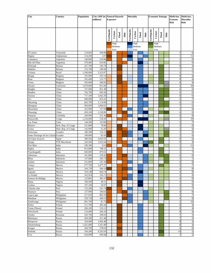
City Country Population City GDP (in
millions)
Multi-haz.
Econom.
Risk
Multi-haz.
Mortality
Risk
Ea
rth
qu
ak
e
Cy
clo
ne
Flo
od
Sli
de
Ea
rth
qu
ak
e
Cy
clo
ne
Flo
od
Sli
de
Ea
rth
qu
ak
e
Cy
clo
ne
Flo
od
Sli
de
3 High 3 High 3 High
2 Medium 2 Medium 2 Medium
1 Low 1 Low 1 Low
Natural Hazards
Exposure
Mortality Economic Damage
El Limon Venezuela 119,602 438.08 2 0 2 2 2 0 2 1 1 0 1 1 5 8
Baglan Afghanistan 114,200 2.07 3 0 2 2 3 0 1 2 1 0 1 1 1 11
Catamarca Argentina 140,000 210.86 2 0 2 0 2 0 2 0 1 0 1 0 3 9
Mar del Plata Argentina 579,483 610.85 0 0 2 2 0 0 3 1 0 0 1 1 3 9
Bobrujsk Belarus 227,700 146.78 0 0 3 0 0 0 2 0 0 0 2 0 8 4
Mahileu Belarus 372,700 189.06 0 0 3 0 0 0 2 0 0 0 2 0 7 5
Goiania Brazil 1,106,000 5,353.07 0 0 2 0 0 0 2 0 0 0 2 0 5 7
Burgas Bulgaria 192,900 203.14 1 0 3 0 1 0 2 0 1 0 2 0 8 4
Ruse Bulgaria 165,400 133.75 1 0 3 0 1 0 2 0 1 0 2 0 8 4
Varna Bulgaria 293,600 280.83 1 0 3 2 1 0 2 1 1 0 2 4 8 4
Douala Cameroon 1,670,000 812.60 0 0 2 2 0 0 3 3 0 0 1 4 2 10
Bengbu China 747,600 851.48 0 0 2 2 0 0 2 2 0 0 2 2 6 6
Huaibei China 762,700 843.26 0 0 2 2 0 0 2 2 0 0 2 2 6 6
Jiaozuo China 717,100 1,042.20 0 0 2 2 0 0 2 3 0 0 2 2 6 6
Jixi China 949,000 655.41 0 0 2 0 0 0 2 0 0 0 2 0 5 7
Maoming China 663,700 1,114.84 0 0 2 2 0 0 2 2 0 0 2 2 6 6
Shaoguan China 494,600 1,694.61 0 0 2 2 0 0 2 2 0 0 2 2 7 5
Shizuishan China 323,900 157.09 3 0 2 0 2 0 2 0 1 0 1 0 3 9
Zhaoqing China 459,100 1,130.00 0 0 2 3 0 0 2 3 0 0 2 3 6 6
Popayan Colombia 204,900 251.36 2 0 0 2 2 0 0 1 1 0 0 1 4 8
Brazzaville Congo 1,234,000 518.20 0 0 2 2 0 0 3 3 0 0 1 4 2 10
Las Tunas Cuba 144,300 310.84 1 0 0 0 1 0 0 0 1 0 0 0 5 7
Bukavu Dem. Rep. of Congo 231,800 78.80 1 0 3 0 1 0 3 0 1 0 1 0 3 9
Goma Dem. Rep. of Congo 142,900 55.20 1 0 3 2 1 0 3 1 1 0 1 4 3 9
Portoviejo Ecuador 180,300 125.15 3 0 2 3 2 0 1 2 1 0 1 2 3 9
Santo Domingo de los ColoradosEcuador 189,800 83.43 3 0 2 3 2 0 1 3 1 0 1 2 3 9
Al-Uqsor (Luxor) Egypt 360,503 3,035.52 0 0 2 0 0 0 2 0 0 0 2 0 6 6
Skopje FYR Macedonia 520,500 1,022.04 1 0 2 2 1 0 1 2 2 0 2 0 8 4
Port Blair India 100,186 0.63 2 0 0 2 2 0 0 3 1 0 0 1 1 11
Rajkot India 913,000 798.31 0 0 2 0 0 0 2 0 0 0 2 0 5 7
Tiruchirppalli India 820,000 879.53 0 0 2 0 0 0 2 0 0 0 2 0 5 7
Adiwerna Indonesia 101,800 529.42 2 0 2 3 1 0 1 2 1 0 2 2 6 6
Blitar Indonesia 137,600 292.73 2 0 2 2 1 0 1 2 1 0 1 2 5 7
Jember Indonesia 231,800 547.20 2 0 0 2 2 0 0 2 1 0 0 2 4 8
Celaya Mexico 277,750 1,477.27 0 0 2 2 0 0 2 1 0 0 2 1 5 7
Iguala Mexico 104,759 306.10 3 0 2 3 2 0 2 1 1 0 1 1 4 8
Irapuato Mexico 319,148 826.74 0 0 2 2 0 0 3 1 0 0 1 1 4 8
La Piedad Mexico 162,954 256.71 1 0 2 2 2 0 2 1 1 0 1 1 3 9
Zamora de Hidalgo Mexico 122,881 385.37 2 0 2 3 2 0 2 1 1 0 1 1 4 8
Bama Nigeria 100,500 40.51 0 0 3 0 0 0 3 0 0 0 1 0 3 9
Gashua Nigeria 107,100 56.07 0 0 3 0 0 0 3 0 0 0 1 0 3 9
Chincha Alta Peru 125,200 241.74 3 0 2 0 2 0 1 0 1 0 1 0 5 7
Huanuco Peru 137,900 180.65 2 0 2 3 1 0 1 2 1 0 1 2 4 8
Lapu-Lapu Philippines 217,019 883.76 2 0 0 2 2 0 0 2 1 0 0 2 5 7
Mandaue Philippines 259,728 449.13 2 0 0 3 2 0 0 2 1 0 0 2 4 8
Zamboanga Philippines 601,794 81.75 2 0 0 0 2 0 0 0 1 0 0 0 2 10
Kielce Poland 211,700 485.44 0 0 3 0 0 0 2 0 0 0 2 0 8 4
Torun (Thorn) Poland 206,100 533.13 0 0 3 0 0 0 2 0 0 0 2 0 8 4
Wloclawek Poland 123,400 426.10 0 0 3 0 0 0 2 0 0 0 2 0 8 4
Oradea Romania 220,700 298.03 0 0 3 0 0 0 2 0 0 0 2 0 7 5
Beboksary Russia 459,200 411.46 0 0 3 0 0 0 2 0 0 0 2 0 7 5
Berepovec Russia 324,400 1,064.48 0 0 3 0 0 0 2 0 0 0 2 0 8 4
Jekaterinburg Russia 1,431,000 3,351.89 0 0 2 0 0 0 2 0 0 0 2 0 8 4
Kurgan Russia 364,700 278.03 0 0 3 0 0 0 2 0 0 0 2 0 6 6
Podolsk Russia 194,300 9,102.64 0 0 2 0 0 0 1 0 0 0 3 0 10 2
Tver Russia 454,900 604.68 0 0 3 0 0 0 2 0 0 0 2 0 7 5
132
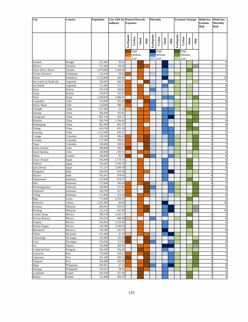
City Country Population City GDP (in
millions)
Multi-haz.
Econom.
Risk
Multi-haz.
Mortality
Risk
Ea
rth
qu
ak
e
Cy
clo
ne
Flo
od
Sli
de
Ea
rth
qu
ak
e
Cy
clo
ne
Flo
od
Sli
de
Ea
rth
qu
ak
e
Cy
clo
ne
Flo
od
Sli
de
3 High 3 High 3 High
2 Medium 2 Medium 2 Medium
1 Low 1 Low 1 Low
Natural Hazards
Exposure
Mortality Economic Damage
Kaolack Senegal 221,400 95.62 0 0 3 0 0 0 3 0 0 0 1 0 3 9
Mtwara Tanzania 131,400 69.56 0 0 3 2 0 0 3 1 0 0 1 4 3 9
Kyyiv (Kiev, Kiew) Ukraine 2,670,000 1,364.94 0 0 2 0 0 0 2 0 0 0 2 0 7 5
Termiz (Termez) Uzbekistan 124,100 59.83 2 0 2 0 1 0 2 0 1 0 1 0 5 7
Harare Zimbabwe 1,752,000 320.60 0 0 2 0 0 0 3 0 0 0 1 0 2 10
San Carlos de Bariloche Argentina 105,093 448.33 2 0 0 3 1 0 0 2 1 0 0 1 4 7
San Rafael Argentina 111,066 153.67 2 0 2 0 1 0 2 0 1 0 1 0 3 8
Sucre Bolivia 192,238 148.88 2 0 2 0 2 0 1 0 1 0 1 0 3 8
Tarija Bolivia 135,679 152.97 2 0 2 0 1 0 1 0 1 0 1 0 4 7
Natal Brazil 1,038,830 2,998.95 0 0 2 2 0 0 2 2 0 0 1 2 4 7
Coquimbo Chile 133,000 292.08 3 0 0 3 2 0 0 1 1 0 0 1 3 8
Puerto Montt Chile 134,000 488.75 2 0 0 2 2 0 0 1 1 0 0 1 4 7
Chengde China 417,200 61.26 1 0 2 2 2 0 2 2 1 0 1 1 2 9
Deyang China 594,400 762.81 0 0 2 2 0 0 2 2 0 0 2 2 6 5
Guangyuan China 867,100 329.12 0 0 2 2 0 0 2 3 0 0 1 2 4 7
Huizhou China 358,700 1,344.60 0 0 2 2 0 0 2 1 0 0 2 2 7 4
Mudanjiang China 801,000 601.67 0 0 2 0 0 0 2 0 0 0 2 0 5 6
Tieling China 419,700 835.33 0 0 2 2 0 0 2 2 0 0 2 2 6 5
Zaoyang China 1,121,000 450.12 0 0 2 2 0 0 2 2 0 0 1 1 4 7
Cartago Colombia 130,500 186.63 2 0 2 3 1 0 1 2 1 0 1 2 4 7
Girardot Colombia 117,000 199.29 2 0 2 3 1 0 1 2 1 0 1 2 4 7
Tunja Colombia 109,600 169.64 2 0 0 3 1 0 0 2 1 0 0 2 4 7
Palma Soriano Cuba 108,400 199.21 3 0 0 3 1 0 0 1 1 0 0 2 4 7
Sancti Spiritus Cuba 120,800 339.35 1 0 2 2 1 0 1 1 1 0 1 1 5 6
Manta Ecuador 168,800 95.97 3 0 0 3 2 0 0 2 1 0 0 1 3 8
Asyut (Assiut) Egypt 343,498 1,770.74 0 0 2 0 0 0 2 0 0 0 2 0 5 6
Mallawi Egypt 119,283 3,796.70 0 0 2 0 0 0 2 0 0 0 2 0 7 4
Qina (Kena) Egypt 171,275 3,288.59 0 0 2 0 0 0 2 0 0 0 2 0 7 4
Mangalore India 538,560 643.96 0 0 2 2 0 0 2 3 0 0 1 1 4 7
Mysore India 742,261 478.65 0 0 2 0 0 0 2 0 0 0 1 0 4 7
Banjarmasin Indonesia 553,000 874.75 0 0 2 0 0 0 2 0 0 0 2 0 6 5
Palu Indonesia 175,900 196.94 2 0 2 3 1 0 1 2 1 0 1 2 4 7
Pematangsiantar Indonesia 240,800 321.86 2 0 0 3 2 0 0 2 1 0 0 2 3 8
Sukabumi Indonesia 140,700 437.15 2 0 0 3 1 0 0 2 1 0 0 2 4 7
Talang Indonesia 131,800 419.40 2 0 2 2 1 0 1 1 1 0 1 2 5 6
Riga Latvia 775,000 3,104.57 0 0 2 0 0 0 1 0 0 0 2 0 8 3
Monrovia Liberia 1,347,600 60.82 0 0 2 0 0 0 3 0 0 0 1 0 1 10
Kuantan Malaysia 283,041 920.63 0 0 2 3 0 0 2 3 0 0 1 4 2 9
Kuching Malaysia 152,310 437.89 0 0 2 3 0 0 2 3 0 0 1 4 1 10
Ciudad Acuna Mexico 108,159 2,420.17 0 0 2 0 0 0 2 0 0 0 2 0 6 5
Nicolas Romero Mexico 216,192 468.44 1 0 0 0 2 0 0 0 1 0 0 0 3 8
Nogales Mexico 156,854 1,722.09 0 0 2 0 0 0 2 0 0 0 2 0 5 6
Piedras Negras Mexico 126,386 2,248.93 0 0 2 0 0 0 2 0 0 0 2 0 6 5
Marrakech Morocco 736,500 762.79 0 0 2 0 0 0 3 0 0 0 1 0 3 8
Thaton Myanmar 101,300 41.50 1 0 2 2 1 0 2 3 1 0 1 0 4 7
Chinandega Nicaragua 120,400 143.48 3 0 0 3 1 0 0 1 1 0 0 1 4 7
Leon Nicaragua 153,200 113.90 3 0 0 3 2 0 0 2 1 0 0 2 3 8
Jos Nigeria 722,900 300.00 0 0 2 2 0 0 3 3 0 0 1 4 2 9
Ciudad del Este Paraguay 254,300 556.40 0 0 3 2 0 0 2 1 0 0 1 1 4 7
Ayacuchu Peru 110,600 158.21 2 0 2 3 1 0 1 2 1 0 1 2 4 7
Cajamarca Peru 101,200 160.21 3 0 0 3 1 0 0 2 1 0 0 2 4 7
Tarapoto Peru 105,900 202.08 2 0 2 3 1 0 1 2 1 0 1 2 4 7
Iligan Philippines 285,061 67.26 2 0 2 3 2 0 2 3 1 0 1 2 2 9
Santiago Philippines 110,531 58.54 1 0 3 2 1 0 2 1 1 0 1 1 4 7
Grudziadz Poland 102,500 251.90 0 0 3 0 0 0 2 0 0 0 2 0 7 4
Radom Poland 231,600 506.97 0 0 3 0 0 0 2 0 0 0 2 0 7 4
133

City Country Population City GDP (in
millions)
Multi-haz.
Econom.
Risk
Multi-haz.
Mortality
Risk
Ea
rth
qu
ak
e
Cy
clo
ne
Flo
od
Sli
de
Ea
rth
qu
ak
e
Cy
clo
ne
Flo
od
Sli
de
Ea
rth
qu
ak
e
Cy
clo
ne
Flo
od
Sli
de
3 High 3 High 3 High
2 Medium 2 Medium 2 Medium
1 Low 1 Low 1 Low
Natural Hazards
Exposure
Mortality Economic Damage
Dzerdinsk Russia 277,100 746.49 0 0 3 0 0 0 2 0 0 0 2 0 7 4
Nidnekamsk Russia 223,400 559.55 0 0 3 0 0 0 2 0 0 0 2 0 7 4
Novokujbysevsk Russia 116,200 700.47 0 0 3 0 0 0 1 0 0 0 2 0 8 3
Novosibirsk Russia 1,478,000 2,100.85 0 0 2 0 0 0 2 0 0 0 2 0 7 4
Syzran Russia 186,900 572.79 0 0 3 0 0 0 2 0 0 0 2 0 7 4
Voloskij Russia 286,900 688.19 0 0 3 0 0 0 2 0 0 0 2 0 7 4
Freetown Sierra Leone 1,013,400 190.27 0 0 0 3 0 0 0 3 0 0 4 0 0 11
Abarah Sudan 110,500 174.57 0 0 3 0 0 0 2 0 0 0 1 0 4 7
Mwanza Tanzania 1,155,000 240.40 0 0 2 0 0 0 3 0 0 0 1 0 2 9
Carupano Venezuela 121,892 278.62 3 0 0 3 2 0 0 1 1 0 0 1 3 8
Cua Venezuela 101,868 216.71 2 0 2 2 1 0 2 1 1 0 1 1 3 8
Mariara Venezuela 101,115 182.18 2 0 2 2 1 0 2 1 1 0 1 1 3 8
Thai Nguyen Vietnam 131,500 58.12 0 0 2 2 0 0 2 3 0 0 2 4 5 6
La Rioja Argentina 138,074 161.85 2 0 0 0 2 0 0 0 1 0 0 0 2 8
Brest Belarus 304,200 153.33 0 0 3 0 0 0 2 0 0 0 2 0 6 4
Mazyr Belarus 109,000 106.92 0 0 3 0 0 0 1 0 0 0 2 0 7 3
Sarajevo Bosnia and Herzeg. 360,000 330.96 2 0 2 2 1 0 1 2 1 0 1 0 6 4
Juazeiro Brazil 132,796 522.16 0 0 3 0 0 0 2 0 0 0 1 0 4 6
Petropolis Brazil 270,489 8,335.14 0 0 2 2 0 0 2 1 0 0 2 3 6 4
Rio Grande Brazil 179,422 760.43 0 0 3 0 0 0 2 0 0 0 1 0 4 6
Sao Jose dos Campos Brazil 952,000 1,886.27 0 0 2 0 0 0 2 0 0 0 1 0 3 7
Sorocaba Brazil 487,907 4,185.90 0 0 2 2 0 0 2 1 0 0 2 2 5 5
Plovdiv Bulgaria 344,500 373.38 2 0 2 2 1 0 1 2 1 0 1 4 6 4
Ouagadougou Burkina Faso 1,130,000 63.64 0 0 2 0 0 0 3 0 0 0 1 0 1 9
Bangui Central African Republic 636,300 140.32 0 0 2 0 0 0 3 0 0 0 1 0 2 8
Los Angeles Chile 113,000 57.84 3 0 2 3 2 0 2 1 1 0 1 1 2 8
Chaoyang China 450,300 624.01 0 0 2 2 0 0 2 2 0 0 2 1 5 5
Chenzhou China 617,200 331.32 0 0 2 2 0 0 2 2 0 0 1 2 4 6
Jinchang China 190,200 104.63 2 0 2 0 1 0 1 0 1 0 1 0 3 7
Liaoyuan China 451,700 671.25 0 0 2 0 0 0 2 0 0 0 2 0 5 5
Longyan China 451,100 487.38 0 0 2 2 0 0 2 2 0 0 2 1 5 5
Qingyuan China 521,300 567.71 0 0 2 2 0 0 2 2 0 0 2 1 5 5
Xinyu China 775,800 417.47 0 0 2 2 0 0 2 2 0 0 1 1 4 6
Yichun China 871,000 317.71 0 0 2 2 0 0 2 2 0 0 1 1 4 6
Zhaodong China 851,000 380.47 0 0 2 0 0 0 2 0 0 0 1 0 4 6
Maicao Colombia 114,300 197.32 2 0 0 0 1 0 0 0 1 0 0 0 4 6
Ciego de Avila Cuba 118,400 258.35 1 0 0 0 1 0 0 0 1 0 0 0 4 6
Lubumbashi Dem. Rep. of Congo 967,000 37.40 0 0 2 0 0 0 3 0 0 0 1 0 1 9
Mbuji-Mayi Dem. Rep. of Congo 874,700 76.68 0 0 2 2 0 0 3 2 0 0 1 4 1 9
Loja Ecuador 124,000 155.07 2 0 0 3 1 0 0 2 1 0 0 2 3 7
Milagro Ecuador 130,800 139.88 2 0 2 0 1 0 1 0 1 0 1 0 3 7
Quevedo Ecuador 126,900 103.49 2 0 2 3 1 0 1 1 1 0 1 1 3 7
Al-Minya (Minje) Egypt 201,360 2,596.67 0 0 2 0 0 0 2 0 0 0 2 0 6 4
Aswan (Assuan) Egypt 219,017 1,688.48 0 0 2 0 0 0 2 0 0 0 2 0 5 5
Sawhaj (Sohag) Egypt 170,125 2,218.10 0 0 2 0 0 0 2 0 0 0 2 0 6 4
Conakry Guinea 1,824,000 425.75 0 0 0 3 0 0 0 3 0 0 0 4 0 10
La Ceiba Honduras 108,900 162.22 2 0 0 3 1 0 0 2 1 0 0 2 4 6
Ranchi India 862,850 449.11 0 0 2 0 0 0 2 0 0 0 1 0 3 7
Ambon Indonesia 261,300 92.05 3 0 0 3 2 0 0 2 1 0 0 1 2 8
Pontianak Indonesia 492,300 527.59 0 0 2 0 0 0 2 0 0 0 2 0 5 5
Samarinda Indonesia 494,800 648.87 0 0 2 2 0 0 2 2 0 0 2 2 5 5
Ipoh Malaysia 566,211 2,022.51 1 0 2 2 4 0 2 2 4 0 1 4 3 7
Kelang Malaysia 563,173 2,099.42 1 0 2 2 4 0 2 2 4 0 1 4 3 7
Petaling Jaya Malaysia 438,084 4,500.55 1 0 2 2 4 0 2 2 4 0 1 4 4 6
Segou Mali 132,400 54.13 0 0 3 0 0 0 3 0 0 0 1 0 2 8
Ciudad Victoria Mexico 249,029 479.37 0 0 2 2 0 0 2 1 0 0 1 1 3 7
134
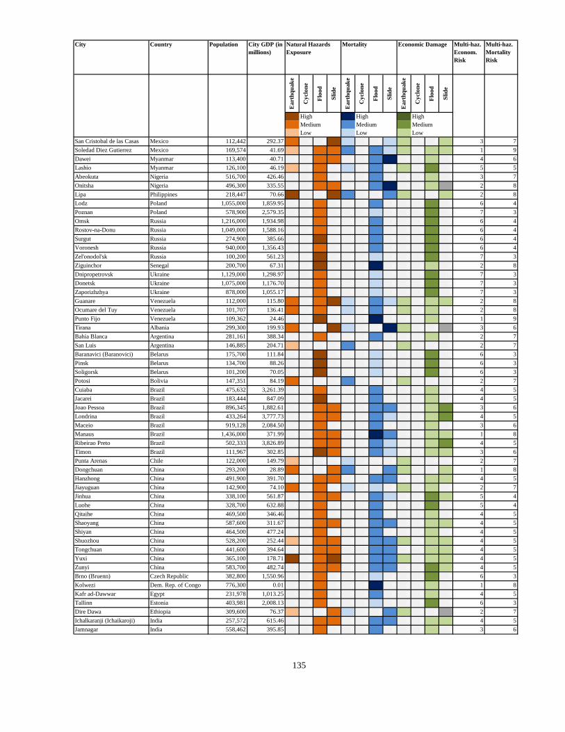
City Country Population City GDP (in
millions)
Multi-haz.
Econom.
Risk
Multi-haz.
Mortality
Risk
Ea
rth
qu
ak
e
Cy
clo
ne
Flo
od
Sli
de
Ea
rth
qu
ak
e
Cy
clo
ne
Flo
od
Sli
de
Ea
rth
qu
ak
e
Cy
clo
ne
Flo
od
Sli
de
3 High 3 High 3 High
2 Medium 2 Medium 2 Medium
1 Low 1 Low 1 Low
Natural Hazards
Exposure
Mortality Economic Damage
San Cristobal de las Casas Mexico 112,442 292.37 2 0 0 3 1 0 0 1 1 0 0 1 3 7
Soledad Diez Gutierrez Mexico 169,574 41.69 1 0 2 2 2 0 2 1 1 0 1 1 1 9
Dawei Myanmar 113,400 40.71 0 0 2 2 0 0 2 3 0 0 1 0 4 6
Lashio Myanmar 126,100 46.19 1 0 2 0 1 0 2 0 1 0 2 0 5 5
Abeokuta Nigeria 516,700 426.46 0 0 2 0 0 0 2 0 0 0 1 0 3 7
Onitsha Nigeria 496,300 335.55 0 0 2 2 0 0 2 3 0 0 1 4 2 8
Lipa Philippines 218,447 70.66 3 0 0 3 2 0 0 2 1 0 0 1 2 8
Lodz Poland 1,055,000 1,859.95 0 0 2 0 0 0 2 0 0 0 2 0 6 4
Poznan Poland 578,900 2,579.35 0 0 2 0 0 0 1 0 0 0 2 0 7 3
Omsk Russia 1,216,000 1,934.98 0 0 2 0 0 0 2 0 0 0 2 0 6 4
Rostov-na-Donu Russia 1,049,000 1,588.16 0 0 2 0 0 0 2 0 0 0 2 0 6 4
Surgut Russia 274,900 385.66 0 0 3 0 0 0 2 0 0 0 2 0 6 4
Voronesh Russia 940,000 1,356.43 0 0 2 0 0 0 2 0 0 0 2 0 6 4
Zel'onodol'sk Russia 100,200 561.23 0 0 3 0 0 0 1 0 0 0 2 0 7 3
Ziguinchor Senegal 200,700 67.31 0 0 3 0 0 0 3 0 0 0 1 0 2 8
Dnipropetrovsk Ukraine 1,129,000 1,298.97 0 0 2 0 0 0 1 0 0 0 2 0 7 3
Donetsk Ukraine 1,075,000 1,176.70 0 0 2 0 0 0 1 0 0 0 2 0 7 3
Zaporizhzhya Ukraine 878,000 1,055.17 0 0 2 0 0 0 1 0 0 0 2 0 7 3
Guanare Venezuela 112,000 115.80 2 0 2 3 1 0 2 1 1 0 1 1 2 8
Ocumare del Tuy Venezuela 101,707 136.41 2 0 2 0 1 0 2 0 1 0 1 0 2 8
Punto Fijo Venezuela 109,362 24.46 0 0 3 0 0 0 3 0 0 0 1 0 1 9
Tirana Albania 299,300 199.93 2 0 0 3 1 0 0 3 1 0 0 4 3 6
Bahia Blanca Argentina 281,161 388.34 0 0 2 0 0 0 2 0 0 0 1 0 2 7
San Luis Argentina 146,885 204.71 1 0 0 0 2 0 0 0 1 0 0 0 2 7
Baranavici (Baranovici) Belarus 175,700 111.84 0 0 3 0 0 0 1 0 0 0 2 0 6 3
Pinsk Belarus 134,700 88.26 0 0 3 0 0 0 1 0 0 0 2 0 6 3
Soligorsk Belarus 101,200 70.05 0 0 3 0 0 0 1 0 0 0 2 0 6 3
Potosi Bolivia 147,351 84.19 2 0 0 0 2 0 0 0 1 0 0 0 2 7
Cuiaba Brazil 475,632 3,261.39 0 0 2 0 0 0 2 0 0 0 1 0 4 5
Jacarei Brazil 183,444 847.09 0 0 3 0 0 0 2 0 0 0 1 0 4 5
Joao Pessoa Brazil 896,345 1,882.61 0 0 2 2 0 0 2 2 0 0 1 2 3 6
Londrina Brazil 433,264 3,777.73 0 0 2 2 0 0 2 1 0 0 1 2 4 5
Maceio Brazil 919,128 2,084.50 0 0 2 0 0 0 2 0 0 0 1 0 3 6
Manaus Brazil 1,436,000 371.99 0 0 2 2 0 0 3 2 0 0 1 1 1 8
Ribeirao Preto Brazil 502,333 3,826.89 0 0 2 2 0 0 2 1 0 0 1 2 4 5
Timon Brazil 111,967 302.85 0 0 3 2 0 0 2 1 0 0 1 1 3 6
Punta Arenas Chile 122,000 149.79 1 0 0 0 1 0 0 0 1 0 0 0 2 7
Dongchuan China 293,200 28.89 2 0 0 2 2 0 0 2 1 0 0 1 1 8
Hanzhong China 491,900 391.70 0 0 2 2 0 0 2 2 0 0 1 1 4 5
Jiayuguan China 142,900 74.10 2 0 2 0 1 0 1 0 1 0 1 0 2 7
Jinhua China 338,100 561.87 0 0 2 2 0 0 2 1 0 0 2 1 5 4
Luohe China 328,700 632.88 0 0 2 0 0 0 2 0 0 0 2 0 5 4
Qitaihe China 469,500 346.46 0 0 2 0 0 0 2 0 0 0 1 0 4 5
Shaoyang China 587,600 311.67 0 0 2 2 0 0 2 2 0 0 1 1 4 5
Shiyan China 464,500 477.24 0 0 2 0 0 0 2 0 0 0 1 0 4 5
Shuozhou China 528,200 252.44 1 0 2 2 0 0 2 2 1 0 1 1 4 5
Tongchuan China 441,600 394.64 0 0 2 2 0 0 2 2 0 0 1 1 4 5
Yuxi China 365,100 178.71 3 0 2 3 0 0 2 2 1 0 1 1 4 5
Zunyi China 583,700 482.74 0 0 2 2 0 0 2 2 0 0 2 1 4 5
Brno (Bruenn) Czech Republic 382,800 1,550.96 0 0 2 0 0 0 1 0 0 0 2 0 6 3
Kolwezi Dem. Rep. of Congo 776,300 0.01 0 0 2 0 0 0 3 0 0 0 1 0 1 8
Kafr ad-Dawwar Egypt 231,978 1,013.25 0 0 2 0 0 0 2 0 0 0 1 0 4 5
Tallinn Estonia 403,981 2,008.13 0 0 2 0 0 0 1 0 0 0 2 0 6 3
Dire Dawa Ethiopia 309,600 76.37 1 0 0 2 1 0 0 2 1 0 0 4 2 7
Ichalkaranji (Ichaikaroji) India 257,572 615.46 0 0 2 2 0 0 2 2 0 0 1 1 4 5
Jamnagar India 558,462 395.85 0 0 2 0 0 0 2 0 0 0 1 0 3 6
135
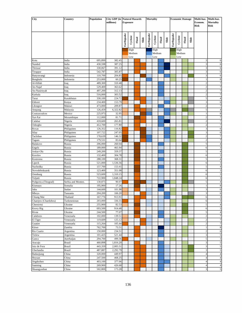
City Country Population City GDP (in
millions)
Multi-haz.
Econom.
Risk
Multi-haz.
Mortality
Risk
Ea
rth
qu
ak
e
Cy
clo
ne
Flo
od
Sli
de
Ea
rth
qu
ak
e
Cy
clo
ne
Flo
od
Sli
de
Ea
rth
qu
ak
e
Cy
clo
ne
Flo
od
Sli
de
3 High 3 High 3 High
2 Medium 2 Medium 2 Medium
1 Low 1 Low 1 Low
Natural Hazards
Exposure
Mortality Economic Damage
Kota India 695,899 382.45 0 0 2 0 0 0 2 0 0 0 1 0 3 6
Nanded India 430,598 387.25 0 0 2 2 0 0 2 3 0 0 1 1 3 6
Thrissur India 330,067 391.12 0 0 2 2 0 0 2 3 0 0 1 1 3 6
Tiruppur India 542,787 305.87 0 0 2 0 0 0 2 0 0 0 1 0 3 6
Banyuwangi Indonesia 110,700 204.85 2 0 0 3 1 0 0 2 1 0 0 2 3 6
Bengkulu Indonesia 253,000 60.25 3 0 0 0 2 0 0 0 1 0 0 0 1 8
Al-Hillah Iraq 489,300 310.48 0 0 2 0 0 0 2 0 0 0 1 0 2 7
An-Najaf Iraq 529,400 363.62 0 0 2 0 0 0 2 0 0 0 1 0 2 7
An-Nasiriryah Iraq 497,200 312.13 0 0 2 0 0 0 2 0 0 0 1 0 2 7
Karbala Iraq 516,000 303.52 0 0 2 0 0 0 2 0 0 0 1 0 2 7
Taraz Kazakhstan 330,100 224.72 3 0 2 2 1 0 1 1 1 0 1 4 5 4
Eldoret Kenya 234,400 153.79 1 0 0 2 1 0 0 2 1 0 0 4 3 6
Lilongwe Malawi 473,000 209.87 0 0 2 0 0 0 2 0 0 0 1 0 2 7
Ampang Malaysia 126,459 6,322.82 1 0 2 2 4 0 1 2 4 0 2 4 5 4
Coatzacoalcos Mexico 225,973 32.95 1 0 0 3 2 0 0 2 1 0 0 1 1 8
Xai-Xai Mozambique 112,000 81.71 0 0 3 2 0 0 2 1 0 0 1 0 2 7
Calabar Nigeria 418,600 265.81 0 0 2 2 0 0 2 3 0 0 1 4 2 7
Oshogbo Nigeria 412,700 177.80 0 0 2 0 0 0 2 0 0 0 1 0 2 7
Roxas Philippines 126,352 116.82 2 0 2 3 1 0 1 2 1 0 1 1 3 6
Silay Philippines 107,722 247.05 2 0 0 3 1 0 0 2 1 0 0 2 3 6
Tacloban Philippines 178,639 146.32 3 0 0 3 2 0 0 2 1 0 0 2 2 7
Tagum Philippines 179,531 83.64 3 0 0 2 2 0 0 1 1 0 0 1 2 7
Balakovo Russia 206,000 260.04 0 0 3 0 0 0 2 0 0 0 2 0 5 4
Engels Russia 189,000 465.94 0 0 3 0 0 0 1 0 0 0 2 0 6 3
Joskar-Ola Russia 249,200 359.37 0 0 3 0 0 0 2 0 0 0 2 0 5 4
Korolov Russia 132,400 304.78 0 0 3 0 0 0 1 0 0 0 2 0 6 3
Kostroma Russia 288,100 368.31 0 0 3 0 0 0 2 0 0 0 2 0 5 4
Lipeck Russia 521,000 1,536.56 0 0 2 0 0 0 1 0 0 0 2 0 6 3
Nachodka Russia 157,700 153.41 0 0 3 0 0 0 2 0 0 0 2 0 5 4
Novodeboksarsk Russia 123,400 351.08 0 0 3 0 0 0 1 0 0 0 2 0 6 3
Orenburg Russia 523,600 1,310.15 0 0 2 0 0 0 1 0 0 0 2 0 6 3
Toljatti Russia 722,900 1,848.24 0 0 2 0 0 0 1 0 0 0 2 0 6 3
Podgorica (Titograd) Serbia and Monten. 130,875 90.07 2 0 3 3 1 0 1 2 1 0 2 4 5 4
Kismayu Somalia 195,900 17.26 0 0 3 0 0 0 3 0 0 0 1 0 1 8
Juba Sudan 144,600 101.98 1 0 2 0 1 0 2 0 1 0 1 0 3 6
Mbeya Tanzania 204,200 166.20 1 0 0 2 1 0 0 2 1 0 0 4 3 6
Chiang Mai Thailand 167,776 913.91 0 0 2 2 0 0 1 2 0 0 2 2 6 3
Chaerjew (Chardzhou) Turkmenistan 203,000 336.55 2 0 2 0 1 0 1 0 1 0 1 0 6 3
Chernivtsi Ukraine 255,900 82.53 1 0 3 0 1 0 1 0 1 0 2 0 5 4
Krovy Rig Ukraine 693,500 914.48 0 0 2 0 0 0 1 0 0 0 2 0 6 3
Rivne Ukraine 244,500 77.07 0 0 3 0 0 0 2 0 0 0 2 0 5 4
Calabozo Venezuela 102,000 139.51 1 0 2 0 1 0 2 0 1 0 1 0 2 7
El Tigre Venezuela 119,609 125.12 1 0 0 2 1 0 0 1 1 0 0 1 2 7
Guatire Venezuela 115,264 105.44 2 0 0 2 1 0 0 1 1 0 0 1 2 7
Kitwe Zambia 762,700 73.51 0 0 2 0 0 0 3 0 0 0 1 0 1 8
Rio Cuarto Argentina 150,000 234.51 0 0 2 0 0 0 2 0 0 0 1 0 2 6
Trelew Argentina 101,425 521.44 0 0 2 0 0 0 2 0 0 0 1 0 3 5
Ganca Azerbaijan 294,700 499.36 2 0 0 0 1 0 0 0 1 0 0 0 5 3
Aracaju Brazil 460,898 1,816.20 0 0 2 0 0 0 2 0 0 0 1 0 3 5
Juiz de Fora Brazil 443,359 2,005.51 0 0 2 2 0 0 2 1 0 0 1 2 3 5
Uberlandia Brazil 487,887 2,292.79 0 0 2 2 0 0 2 1 0 0 1 2 3 5
Badaojiang China 320,000 449.97 0 0 2 2 0 0 2 1 0 0 1 1 4 4
Heyuan China 247,500 468.25 0 0 2 2 0 0 2 1 0 0 1 1 4 4
Jingdezhen China 403,100 377.06 0 0 2 2 0 0 2 2 0 0 1 1 4 4
Sanming China 269,900 426.68 0 0 2 2 0 0 2 1 0 0 1 1 4 4
Shuangyashan China 502,800 173.28 0 0 2 0 0 0 2 0 0 0 1 0 3 5
136
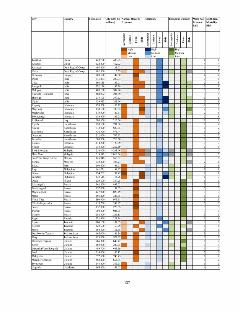
City Country Population City GDP (in
millions)
Multi-haz.
Econom.
Risk
Multi-haz.
Mortality
Risk
Ea
rth
qu
ak
e
Cy
clo
ne
Flo
od
Sli
de
Ea
rth
qu
ak
e
Cy
clo
ne
Flo
od
Sli
de
Ea
rth
qu
ak
e
Cy
clo
ne
Flo
od
Sli
de
3 High 3 High 3 High
2 Medium 2 Medium 2 Medium
1 Low 1 Low 1 Low
Natural Hazards
Exposure
Mortality Economic Damage
Tonghua China 428,700 439.65 0 0 2 0 0 0 2 0 0 0 1 0 4 4
Wuzhou China 328,400 452.02 0 0 2 0 0 0 2 0 0 0 1 0 4 4
Kisangani Dem. Rep. of Congo 497,800 39.72 0 0 2 0 0 0 2 0 0 0 1 0 1 7
Uvira Dem. Rep. of Congo 182,300 9.55 1 0 2 2 1 0 2 1 1 0 1 4 1 7
Debrecen Hungary 209,600 142.00 0 0 3 0 0 0 2 0 0 0 1 0 4 4
Dhule India 341,473 307.74 0 0 2 0 0 0 2 0 0 0 1 0 3 5
Gaya India 394,185 185.01 0 0 2 2 0 0 2 3 0 0 1 1 2 6
Junagadh India 252,138 147.79 0 0 2 2 0 0 2 3 0 0 1 1 2 6
Malegaon India 409,190 392.26 0 0 2 0 0 0 2 0 0 0 1 0 3 5
Raurkela (Rourkela) India 484,292 294.59 0 0 2 0 0 0 2 0 0 0 1 0 3 5
Shimoga India 274,105 307.62 0 0 2 2 0 0 2 3 0 0 1 1 3 5
Ujjain India 429,933 208.26 0 0 2 2 0 0 2 3 0 0 1 1 2 6
Kupang Indonesia 159,300 163.77 2 0 0 2 1 0 0 1 1 0 0 1 2 6
Magelang Indonesia 138,100 199.55 2 0 0 3 1 0 0 2 1 0 0 2 2 6
Mertoyudan Indonesia 119,000 89.87 2 0 0 2 1 0 0 1 1 0 0 1 2 6
Tebingtinggi Indonesia 139,400 189.01 2 0 0 0 1 0 0 0 1 0 0 0 2 6
Ar-Ramadi Iraq 388,300 210.06 0 0 2 0 0 0 2 0 0 0 1 0 2 6
Aqtobe Kazakhstan 253,100 781.36 0 0 2 0 0 0 1 0 0 0 2 0 6 2
Astana Kazakhstan 313,000 609.35 0 0 2 0 0 0 1 0 0 0 2 0 6 2
Earaoanda Kazakhstan 436,900 875.44 0 0 2 0 0 0 1 0 0 0 2 0 6 2
Oskemen Kazakhstan 311,000 707.92 0 0 2 0 0 0 1 0 0 0 2 0 6 2
Pavlodar Kazakhstan 300,500 719.50 0 0 2 0 0 0 1 0 0 0 2 0 6 2
Kaunas Lithuania 414,200 1,120.69 0 0 2 0 0 0 1 0 0 0 2 0 5 3
Vilnius Lithuania 578,300 1,252.39 0 0 2 0 0 0 1 0 0 0 2 0 5 3
Bukit Mertajam Malaysia 210,000 4,208.76 1 0 2 2 4 0 2 1 4 0 1 4 4 4
Shah Alam Malaysia 319,612 2,818.36 1 0 2 2 4 0 2 2 4 0 1 4 3 5
San Pedro Garza Garcia Mexico 125,945 556.57 0 0 2 0 0 0 2 0 0 0 1 0 3 5
Kenitra Morocco 330,200 403.24 0 0 2 2 0 0 2 1 0 0 1 4 2 6
Talara Peru 100,600 45.07 2 0 0 0 1 0 0 0 1 0 0 0 2 6
Bago Philippines 141,721 91.67 2 0 0 0 1 0 0 0 1 0 0 0 2 6
Ormoc Philippines 154,297 37.47 3 0 0 3 1 0 0 2 1 0 0 1 1 7
Pagadian Philippines 142,515 14.26 2 0 0 3 1 0 0 3 1 0 0 1 1 7
Opole Poland 129,500 357.25 0 0 3 0 0 0 1 0 0 0 2 0 5 3
Arkhangelsk Russia 361,800 849.02 0 0 2 0 0 0 1 0 0 0 2 0 5 3
Dimitrovgrad Russia 137,000 191.85 0 0 3 0 0 0 1 0 0 0 2 0 5 3
Magnitogorsk Russia 427,900 1,025.49 0 0 2 0 0 0 1 0 0 0 2 0 5 3
Miass Russia 166,200 333.55 0 0 3 0 0 0 1 0 0 0 2 0 5 3
Nidnij Tagil Russia 390,900 975.91 0 0 2 0 0 0 1 0 0 0 2 0 5 3
Nikolo-Berjozovka Russia 115,700 243.97 0 0 3 0 0 0 1 0 0 0 2 0 5 3
Serov Russia 132,000 228.35 0 0 3 0 0 0 1 0 0 0 2 0 5 3
T'umen' Russia 503,800 941.95 0 0 2 0 0 0 1 0 0 0 2 0 5 3
Ustinov Russia 652,800 1,236.13 0 0 2 0 0 0 1 0 0 0 2 0 5 3
Kigali Rwanda 351,400 229.74 0 0 2 0 0 0 2 0 0 0 1 0 2 6
Arusha Tanzania 160,100 137.35 1 0 0 2 1 0 0 2 1 0 0 4 3 5
Kigoma Tanzania 120,500 55.29 1 0 2 0 1 0 2 0 1 0 1 0 2 6
Moshi Tanzania 188,300 118.55 1 0 0 2 1 0 0 2 1 0 0 4 3 5
Dashhowuz (Tasauz) Turkmenistan 165,000 196.54 2 0 2 0 1 0 1 0 1 0 1 0 5 3
Mary Turkmenistan 123,000 321.87 2 0 2 0 1 0 1 0 1 0 1 0 6 2
Dniprodzerzhynsk Ukraine 266,300 649.47 0 0 2 0 0 0 1 0 0 0 2 0 6 2
Kerch Ukraine 160,900 240.65 2 0 2 0 1 0 1 0 1 0 1 0 5 3
Luhansk (Vorosilovgrad) Ukraine 459,700 633.69 0 0 2 0 0 0 1 0 0 0 2 0 6 2
Lutsk Ukraine 216,800 86.12 0 0 3 0 0 0 1 0 0 0 2 0 5 3
Makiyivka Ukraine 377,500 743.43 0 0 2 0 0 0 1 0 0 0 2 0 6 2
Mariupol' (Zdanov) Ukraine 484,400 654.85 0 0 2 0 0 0 1 0 0 0 2 0 6 2
Sevastopol Ukraine 344,400 359.61 2 0 0 0 1 0 0 0 1 0 0 0 5 3
Urgench Uzbekistan 165,400 63.02 2 0 0 0 1 0 0 0 1 0 0 0 4 4
137
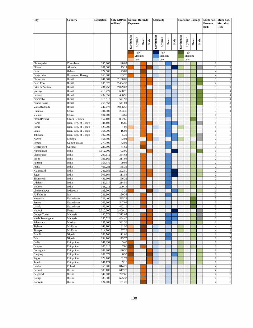
City Country Population City GDP (in
millions)
Multi-haz.
Econom.
Risk
Multi-haz.
Mortality
Risk
Ea
rth
qu
ak
e
Cy
clo
ne
Flo
od
Sli
de
Ea
rth
qu
ak
e
Cy
clo
ne
Flo
od
Sli
de
Ea
rth
qu
ak
e
Cy
clo
ne
Flo
od
Sli
de
3 High 3 High 3 High
2 Medium 2 Medium 2 Medium
1 Low 1 Low 1 Low
Natural Hazards
Exposure
Mortality Economic Damage
Chitungwiza Zimbabwe 390,600 148.07 0 0 2 0 0 0 2 0 0 0 1 0 2 6
Elbasan Albania 101,300 75.11 2 0 2 3 1 0 1 3 1 0 1 4 3 4
Orsa Belarus 124,500 73.82 0 0 3 0 0 0 1 0 0 0 1 0 4 3
Banja Luka Bosnia and Herzeg. 160,000 133.78 2 0 2 0 1 0 1 0 1 0 1 0 4 3
Blumenau Brazil 241,987 2,108.89 0 0 2 2 0 0 1 1 0 0 1 2 3 4
Cabo Frio Brazil 106,326 2,434.30 0 0 2 2 0 0 1 1 0 0 1 2 4 3
Feira de Santana Brazil 431,458 2,029.02 0 0 2 0 0 0 2 0 0 0 1 0 3 4
Ipatinga Brazil 210,777 1,668.76 0 0 2 2 0 0 1 1 0 0 1 2 3 4
Limeira Brazil 237,959 1,436.95 0 0 2 2 0 0 1 1 0 0 1 2 3 4
Piracicaba Brazil 316,518 1,571.99 0 0 2 2 0 0 2 1 0 0 1 2 3 4
Ponta Grossa Brazil 266,552 1,541.01 0 0 2 2 0 0 2 1 0 0 1 2 3 4
Volta Redonda Brazil 242,773 2,096.55 0 0 2 0 0 0 1 0 0 0 1 0 3 4
Huaihua China 301,500 293.36 0 0 2 0 0 0 2 0 0 0 1 0 3 4
Yichun China 904,000 53.69 0 0 2 0 0 0 2 0 0 0 1 0 1 6
Plzen (Pilsen) Czech Republic 167,100 882.65 0 0 2 0 0 0 1 0 0 0 2 0 5 2
Boma Dem. Rep. of Congo 341,100 15.80 0 0 2 2 0 0 2 2 0 0 1 4 1 6
Bunia Dem. Rep. of Congo 123,700 1.08 1 0 2 0 1 0 2 0 1 0 1 0 1 6
Likasi Dem. Rep. of Congo 364,700 16.03 0 0 2 0 0 0 2 0 0 0 1 0 1 6
Tshikapa Dem. Rep. of Congo 302,300 5.22 0 0 2 2 0 0 2 2 0 0 1 4 1 6
Nazret Ethiopia 161,800 62.01 1 0 0 2 1 0 0 2 1 0 0 4 2 5
Bissau Guinea-Bissau 279,900 42.02 0 0 2 0 0 0 2 0 0 0 1 0 1 6
Georgetown Guyana 223,900 41.62 0 0 3 0 0 0 2 0 0 0 1 0 1 6
Aurangabad India 1,012,000 793.90 0 0 0 2 0 0 0 3 0 0 0 2 1 6
Chandrapur India 297,612 364.64 0 0 2 0 0 0 2 0 0 0 1 0 3 4
Erode India 391,169 217.03 0 0 2 0 0 0 2 0 0 0 1 0 2 5
Jalgaon India 368,579 99.94 0 0 2 0 0 0 2 0 0 0 1 0 2 5
Jhansi India 463,281 165.26 0 0 2 0 0 0 2 0 0 0 1 0 2 5
Nizamabad India 286,956 202.50 0 0 2 2 0 0 2 3 0 0 1 1 2 5
Sagar India 309,164 111.54 0 0 2 2 0 0 2 3 0 0 1 1 2 5
Tirunelveli India 431,603 196.22 0 0 2 0 0 0 2 0 0 0 1 0 2 5
Udaipur India 389,317 214.55 0 0 2 0 0 0 2 0 0 0 1 0 2 5
Vellore India 388,211 200.14 0 0 2 0 0 0 2 0 0 0 1 0 2 5
Lhokseumawe Indonesia 135,000 43.26 2 0 0 3 1 0 0 2 1 0 0 1 1 6
Al-Fallujah Iraq 221,600 150.35 0 0 2 0 0 0 2 0 0 0 1 0 2 5
Kostanay Kazakhstan 221,400 595.28 0 0 2 0 0 0 1 0 0 0 2 0 5 2
Semey Kazakhstan 269,600 547.03 0 0 2 0 0 0 1 0 0 0 2 0 5 2
Uralsk Kazakhstan 195,500 462.15 0 0 2 0 0 0 1 0 0 0 2 0 5 2
Nairobi Kenya 2,310,000 2,809.10 0 0 0 2 0 0 0 3 0 0 0 4 0 7
George Town Malaysia 180,573 2,312.07 0 0 2 2 0 0 2 2 0 0 1 4 3 4
Kuala Terengganu Malaysia 250,528 1,484.40 0 0 2 2 0 0 2 2 0 0 1 4 2 5
Salamanca Mexico 137,000 391.38 0 0 2 2 0 0 2 1 0 0 1 1 2 5
Tighina Moldova 148,100 61.95 1 0 3 0 1 0 1 0 1 0 1 0 4 3
Tiraspol' Moldova 214,700 57.25 1 0 3 0 1 0 1 0 1 0 1 0 4 3
Bauchi Nigeria 283,700 111.08 0 0 2 0 0 0 2 0 0 0 1 0 1 6
Ede Nigeria 234,100 173.75 0 0 2 0 0 0 2 0 0 0 1 0 2 5
Cadiz Philippines 141,954 5.43 2 0 0 0 1 0 0 0 1 0 0 0 1 6
Calapan Philippines 105,910 7.68 3 0 2 0 1 0 1 0 1 0 1 0 1 6
Dumaguete Philippines 102,265 126.36 2 0 0 2 1 0 0 1 1 0 0 1 2 5
Gingoog Philippines 102,379 6.55 3 0 0 3 1 0 0 2 1 0 0 1 1 6
Sagay Philippines 129,765 31.77 2 0 0 2 1 0 0 1 1 0 0 1 1 6
Toledo Philippines 141,174 39.10 2 0 0 2 1 0 0 1 1 0 0 1 1 6
Lublin Poland 356,000 814.27 0 0 2 0 0 0 1 0 0 0 1 0 4 3
Barnaul Russia 580,100 617.25 0 0 2 0 0 0 1 0 0 0 1 0 4 3
Belgorod Russia 342,000 727.66 0 0 2 0 0 0 1 0 0 0 1 0 4 3
Kaluga Russia 339,300 625.33 0 0 2 0 0 0 1 0 0 0 1 0 4 3
Kamysin Russia 124,600 161.27 0 0 3 0 0 0 1 0 0 0 1 0 4 3
138
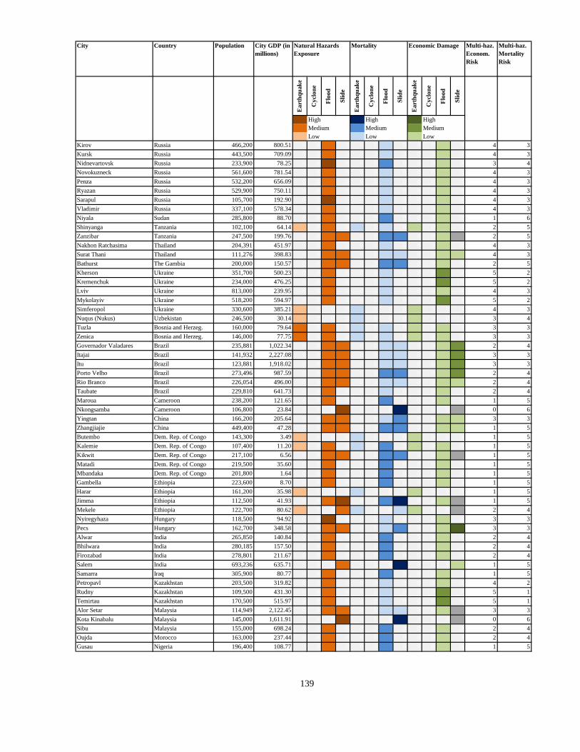
City Country Population City GDP (in
millions)
Multi-haz.
Econom.
Risk
Multi-haz.
Mortality
Risk
Ea
rth
qu
ak
e
Cy
clo
ne
Flo
od
Sli
de
Ea
rth
qu
ak
e
Cy
clo
ne
Flo
od
Sli
de
Ea
rth
qu
ak
e
Cy
clo
ne
Flo
od
Sli
de
3 High 3 High 3 High
2 Medium 2 Medium 2 Medium
1 Low 1 Low 1 Low
Natural Hazards
Exposure
Mortality Economic Damage
Kirov Russia 466,200 800.51 0 0 2 0 0 0 1 0 0 0 1 0 4 3
Kursk Russia 443,500 709.09 0 0 2 0 0 0 1 0 0 0 1 0 4 3
Nidnevartovsk Russia 233,900 78.25 0 0 3 0 0 0 2 0 0 0 1 0 3 4
Novokuzneck Russia 561,600 781.54 0 0 2 0 0 0 1 0 0 0 1 0 4 3
Penza Russia 532,200 656.09 0 0 2 0 0 0 1 0 0 0 1 0 4 3
Ryazan Russia 529,900 750.11 0 0 2 0 0 0 1 0 0 0 1 0 4 3
Sarapul Russia 105,700 192.90 0 0 3 0 0 0 1 0 0 0 1 0 4 3
Vladimir Russia 337,100 578.34 0 0 2 0 0 0 1 0 0 0 1 0 4 3
Niyala Sudan 285,800 88.70 0 0 2 0 0 0 2 0 0 0 1 0 1 6
Shinyanga Tanzania 102,100 64.14 1 0 2 0 1 0 1 0 1 0 1 0 2 5
Zanzibar Tanzania 247,500 199.76 0 0 2 2 0 0 2 2 0 0 1 4 2 5
Nakhon Ratchasima Thailand 204,391 451.97 0 0 2 0 0 0 1 0 0 0 1 0 4 3
Surat Thani Thailand 111,276 398.83 0 0 2 2 0 0 1 1 0 0 1 1 4 3
Bathurst The Gambia 200,000 150.57 0 0 2 2 0 0 2 2 0 0 1 0 2 5
Kherson Ukraine 351,700 500.23 0 0 2 0 0 0 1 0 0 0 2 0 5 2
Kremenchuk Ukraine 234,000 476.25 0 0 2 0 0 0 1 0 0 0 2 0 5 2
Lviv Ukraine 813,000 239.95 0 0 2 0 0 0 1 0 0 0 1 0 4 3
Mykolayiv Ukraine 518,200 594.97 0 0 2 0 0 0 1 0 0 0 2 0 5 2
Simferopol Ukraine 330,600 385.21 1 0 0 0 1 0 0 0 1 0 0 0 4 3
Nuqus (Nukus) Uzbekistan 246,500 30.14 1 0 0 0 1 0 0 0 1 0 0 0 3 4
Tuzla Bosnia and Herzeg. 160,000 79.64 2 0 2 0 1 0 1 0 1 0 1 0 3 3
Zenica Bosnia and Herzeg. 146,000 77.75 2 0 2 0 1 0 1 0 1 0 1 0 3 3
Governador Valadares Brazil 235,881 1,022.34 0 0 2 2 0 0 1 1 0 0 1 2 2 4
Itajai Brazil 141,932 2,227.08 0 0 2 2 0 0 1 1 0 0 1 2 3 3
Itu Brazil 123,881 1,918.02 0 0 2 2 0 0 1 1 0 0 1 2 3 3
Porto Velho Brazil 273,496 987.59 0 0 2 2 0 0 2 2 0 0 1 2 2 4
Rio Branco Brazil 226,054 496.00 0 0 2 2 0 0 1 1 0 0 1 1 2 4
Taubate Brazil 229,810 641.73 0 0 2 0 0 0 1 0 0 0 1 0 2 4
Maroua Cameroon 238,200 121.65 0 0 2 0 0 0 2 0 0 0 1 0 1 5
Nkongsamba Cameroon 106,800 23.84 0 0 0 3 0 0 0 3 0 0 0 4 0 6
Yingtan China 166,200 205.64 0 0 2 2 0 0 1 2 0 0 1 1 3 3
Zhangjiajie China 449,400 47.28 0 0 2 2 0 0 2 2 0 0 1 1 1 5
Butembo Dem. Rep. of Congo 143,300 3.49 1 0 0 0 1 0 0 0 1 0 0 0 1 5
Kalemie Dem. Rep. of Congo 107,400 11.20 1 0 2 0 1 0 2 0 1 0 1 0 1 5
Kikwit Dem. Rep. of Congo 217,100 6.56 0 0 2 2 0 0 2 2 0 0 1 4 1 5
Matadi Dem. Rep. of Congo 219,500 35.60 0 0 2 0 0 0 2 0 0 0 1 0 1 5
Mbandaka Dem. Rep. of Congo 201,800 1.64 0 0 2 0 0 0 2 0 0 0 1 0 1 5
Gambella Ethiopia 223,600 8.70 0 0 2 0 0 0 2 0 0 0 1 0 1 5
Harar Ethiopia 161,200 35.98 1 0 0 0 1 0 0 0 1 0 0 0 1 5
Jimma Ethiopia 112,500 41.93 0 0 2 3 0 0 2 3 0 0 1 4 1 5
Mekele Ethiopia 122,700 80.62 1 0 0 2 1 0 0 1 1 0 0 4 2 4
Nyiregyhaza Hungary 118,500 94.92 0 0 3 0 0 0 1 0 0 0 1 0 3 3
Pecs Hungary 162,700 348.58 0 0 2 2 0 0 1 2 0 0 1 3 3 3
Alwar India 265,850 140.84 0 0 2 0 0 0 2 0 0 0 1 0 2 4
Bhilwara India 280,185 157.50 0 0 2 0 0 0 2 0 0 0 1 0 2 4
Firozabad India 278,801 211.67 0 0 2 0 0 0 2 0 0 0 1 0 2 4
Salem India 693,236 635.71 0 0 0 2 0 0 0 3 0 0 0 1 1 5
Samarra Iraq 305,900 80.77 0 0 2 0 0 0 2 0 0 0 1 0 1 5
Petropavl Kazakhstan 203,500 319.82 0 0 2 0 0 0 1 0 0 0 1 0 4 2
Rudny Kazakhstan 109,500 431.30 0 0 2 0 0 0 1 0 0 0 2 0 5 1
Temirtau Kazakhstan 170,500 515.97 0 0 2 0 0 0 1 0 0 0 2 0 5 1
Alor Setar Malaysia 114,949 2,122.45 0 0 2 2 0 0 1 1 0 0 1 4 3 3
Kota Kinabalu Malaysia 145,000 1,611.91 0 0 0 3 0 0 0 3 0 0 0 4 0 6
Sibu Malaysia 155,000 698.24 0 0 2 0 0 0 2 0 0 0 1 0 2 4
Oujda Morocco 163,000 237.44 0 0 2 0 0 0 2 0 0 0 1 0 2 4
Gusau Nigeria 196,400 108.77 0 0 2 0 0 0 2 0 0 0 1 0 1 5
139

City Country Population City GDP (in
millions)
Multi-haz.
Econom.
Risk
Multi-haz.
Mortality
Risk
Ea
rth
qu
ak
e
Cy
clo
ne
Flo
od
Sli
de
Ea
rth
qu
ak
e
Cy
clo
ne
Flo
od
Sli
de
Ea
rth
qu
ak
e
Cy
clo
ne
Flo
od
Sli
de
3 High 3 High 3 High
2 Medium 2 Medium 2 Medium
1 Low 1 Low 1 Low
Natural Hazards
Exposure
Mortality Economic Damage
Iwo Nigeria 206,600 104.59 0 0 2 0 0 0 2 0 0 0 1 0 1 5
Makurdi Nigeria 243,900 91.70 0 0 2 2 0 0 2 2 0 0 1 4 1 5
Minna Nigeria 262,000 69.55 0 0 2 0 0 0 2 0 0 0 1 0 1 5
Bialystok Poland 285,000 604.64 0 0 2 0 0 0 1 0 0 0 1 0 4 2
Czestochowa Poland 256,500 553.96 0 0 2 0 0 0 1 0 0 0 1 0 4 2
Abakan Russia 169,200 523.51 0 0 2 0 0 0 1 0 0 0 1 0 4 2
Balasicha Russia 132,900 602.42 0 0 2 0 0 0 1 0 0 0 1 0 4 2
Berezniki Russia 181,900 526.61 0 0 2 0 0 0 1 0 0 0 1 0 4 2
Bijsk Russia 225,000 118.80 0 0 3 0 0 0 1 0 0 0 1 0 3 3
Bratsk Russia 457,400 387.24 0 0 2 0 0 0 1 0 0 0 1 0 3 3
Ivanovo Russia 459,200 369.11 0 0 2 0 0 0 1 0 0 0 1 0 3 3
Orel Russia 344,500 502.16 0 0 2 0 0 0 1 0 0 0 1 0 3 3
Orsk Russia 273,900 560.17 0 0 2 0 0 0 1 0 0 0 1 0 4 2
Petrozavodsk Russia 282,100 644.26 0 0 2 0 0 0 1 0 0 0 1 0 4 2
Prokopjevsk Russia 237,300 577.17 0 0 2 0 0 0 1 0 0 0 1 0 4 2
Staryj Oskol Russia 213,800 646.02 0 0 2 0 0 0 1 0 0 0 1 0 4 2
Syktyvkar Russia 229,700 766.31 0 0 2 0 0 0 1 0 0 0 1 0 4 2
Ussurijsk Russia 157,300 140.80 0 0 3 0 0 0 1 0 0 0 1 0 3 3
Nis Serbia and Monten. 182,583 69.07 1 0 2 2 1 0 1 1 1 0 1 4 3 3
Pristina Serbia and Monten. 186,611 65.43 1 0 2 0 1 0 1 0 1 0 1 0 3 3
Ar-Raqqah Syria 207,900 405.07 0 0 2 0 0 0 2 0 0 0 1 0 2 4
Dayr az-Zawr Syria 204,900 340.93 0 0 2 0 0 0 2 0 0 0 1 0 2 4
Geita Tanzania 135,100 156.86 0 0 2 0 0 0 2 0 0 0 1 0 2 4
Tanga Tanzania 202,900 110.69 0 0 2 2 0 0 2 2 0 0 1 4 1 5
Kirovohrad Ukraine 261,700 322.57 0 0 2 0 0 0 1 0 0 0 1 0 4 2
Lysychansk Ukraine 114,300 472.15 0 0 2 0 0 0 1 0 0 0 2 0 5 1
Poltava Ukraine 311,000 351.92 0 0 2 0 0 0 1 0 0 0 1 0 4 2
Sumy Ukraine 292,300 324.43 0 0 2 0 0 0 1 0 0 0 1 0 4 2
Kabwe Zambia 208,200 43.29 0 0 2 0 0 0 2 0 0 0 1 0 1 5
Benguela Angola 129,800 250.75 0 0 2 0 0 0 2 0 0 0 1 0 1 4
Lobito Angola 133,100 409.93 0 0 2 0 0 0 2 0 0 0 1 0 1 4
Grodno Belarus 311,500 158.71 0 0 2 0 0 0 1 0 0 0 1 0 3 2
Vitebsk Belarus 356,000 216.62 0 0 2 0 0 0 1 0 0 0 1 0 3 2
Barra Mansa Brazil 164,963 983.04 0 0 2 0 0 0 1 0 0 0 1 0 2 3
Boa Vista Brazil 196,942 479.37 0 0 2 2 0 0 1 1 0 0 1 1 2 3
Cachoeiro de Itapemirim Brazil 154,771 918.90 0 0 2 2 0 0 1 1 0 0 1 2 2 3
Campos dos Goytacazes Brazil 363,489 304.18 0 0 2 2 0 0 2 1 0 0 1 1 1 4
Caruaru Brazil 217,084 632.64 0 0 2 0 0 0 1 0 0 0 1 0 2 3
Divinopolis Brazil 177,729 739.38 0 0 2 0 0 0 1 0 0 0 1 0 2 3
Ilheus Brazil 161,898 496.97 0 0 2 0 0 0 1 0 0 0 1 0 2 3
Itabuna Brazil 190,888 867.79 0 0 2 0 0 0 1 0 0 0 1 0 2 3
Itapetininga Brazil 111,774 673.70 0 0 2 2 0 0 1 1 0 0 1 2 2 3
Jau Brazil 106,954 641.16 0 0 2 2 0 0 1 1 0 0 1 2 2 3
Jequie Brazil 130,207 501.24 0 0 2 2 0 0 1 1 0 0 1 1 2 3
Macae Brazil 125,118 734.95 0 0 2 0 0 0 1 0 0 0 1 0 2 3
Macapa Brazil 270,077 259.26 0 0 2 0 0 0 2 0 0 0 1 0 1 4
Nossa Senhora do Socorro Brazil 130,255 1,048.17 0 0 2 0 0 0 1 0 0 0 1 0 2 3
Patos de Minas Brazil 111,159 505.08 0 0 2 2 0 0 1 1 0 0 1 1 2 3
Pindamonhangaba Brazil 118,793 1,193.67 0 0 2 2 0 0 1 1 0 0 1 2 2 3
Pocos de Caldas Brazil 130,594 646.46 0 0 2 2 0 0 1 1 0 0 1 2 2 3
Rio Claro Brazil 163,341 1,013.25 0 0 2 2 0 0 1 1 0 0 1 2 2 3
Rondonopolis Brazil 141,660 630.88 0 0 2 2 0 0 1 1 0 0 1 2 2 3
Santarem Brazil 186,518 558.23 0 0 2 2 0 0 1 1 0 0 1 2 2 3
Santos Brazil 1,260,000 6,256.16 0 0 0 2 0 0 0 3 0 0 0 3 2 3
Teresopolis Brazil 114,688 804.61 0 0 2 2 0 0 1 1 0 0 1 2 2 3
Varginha Brazil 103,499 494.96 0 0 2 0 0 0 1 0 0 0 1 0 2 3
140
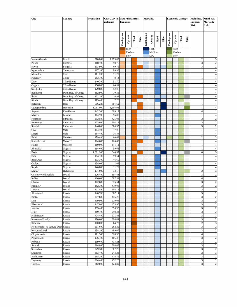
City Country Population City GDP (in
millions)
Multi-haz.
Econom.
Risk
Multi-haz.
Mortality
Risk
Ea
rth
qu
ak
e
Cy
clo
ne
Flo
od
Sli
de
Ea
rth
qu
ak
e
Cy
clo
ne
Flo
od
Sli
de
Ea
rth
qu
ak
e
Cy
clo
ne
Flo
od
Sli
de
3 High 3 High 3 High
2 Medium 2 Medium 2 Medium
1 Low 1 Low 1 Low
Natural Hazards
Exposure
Mortality Economic Damage
Varzea Grande Brazil 210,849 1,299.82 0 0 2 0 0 0 1 0 0 0 1 0 2 3
Pleven Bulgaria 118,700 98.76 1 0 2 0 1 0 1 0 1 0 1 0 3 2
Sliven Bulgaria 103,900 69.75 1 0 2 2 1 0 1 1 1 0 1 0 3 2
Ngaoundere Cameroon 167,100 99.96 0 0 2 0 0 0 2 0 0 0 1 0 1 4
Moundou Chad 111,200 71.29 0 0 2 0 0 0 2 0 0 0 1 0 1 4
Karamay China 263,100 8.14 0 0 2 0 0 0 2 0 0 0 1 0 1 4
Divo Côte d'Ivoire 140,300 51.70 0 0 2 0 0 0 2 0 0 0 1 0 1 4
Gagnoa Côte d'Ivoire 156,800 64.31 0 0 2 0 0 0 2 0 0 0 1 0 1 4
San-Pedro Côte d'Ivoire 129,800 52.07 0 0 2 0 0 0 2 0 0 0 1 0 1 4
Bandundu Dem. Rep. of Congo 112,900 10.36 0 0 2 0 0 0 2 0 0 0 1 0 1 4
Ilebo Dem. Rep. of Congo 101,100 4.94 0 0 2 2 0 0 1 1 0 0 1 4 1 4
Kindu Dem. Rep. of Congo 115,400 7.75 0 0 2 0 0 0 2 0 0 0 1 0 1 4
Belgaum India 506,235 301.62 0 0 0 2 0 0 0 3 0 0 0 1 1 4
Ujungpandang Indonesia 1,051,000 1,594.93 0 0 0 2 0 0 0 3 0 0 0 2 1 4
Atyrao Kazakhstan 142,500 309.17 0 0 2 0 0 0 1 0 0 0 1 0 4 1
Maseru Lesotho 164,700 55.80 0 0 2 0 0 0 2 0 0 0 1 0 1 4
Klaipoda Lithuania 202,500 425.04 0 0 2 0 0 0 1 0 0 0 1 0 3 2
Panevooys Lithuania 133,600 304.17 0 0 2 0 0 0 1 0 0 0 1 0 3 2
Siauliai Lithuania 146,800 304.55 0 0 2 0 0 0 1 0 0 0 1 0 3 2
Gao Mali 104,700 17.06 0 0 2 0 0 0 2 0 0 0 1 0 1 4
Mopti Mali 114,400 36.34 0 0 2 0 0 0 2 0 0 0 1 0 1 4
Boloi Moldova 179,400 60.68 1 0 2 0 1 0 1 0 1 0 1 0 2 3
Ksar-el-Kebir Morocco 124,600 126.49 0 0 2 2 0 0 2 1 0 0 1 4 1 4
Nador Morocco 110,000 141.11 0 0 2 0 0 0 1 0 0 0 1 0 1 4
Abakaliki Nigeria 118,600 59.63 0 0 2 0 0 0 2 0 0 0 1 0 1 4
Benin Nigeria 1,021,900 644.57 0 0 0 2 0 0 0 3 0 0 0 4 0 5
Bida Nigeria 154,100 99.54 0 0 2 0 0 0 2 0 0 0 1 0 1 4
IfonÿOsun Nigeria 103,300 46.69 0 0 2 0 0 0 2 0 0 0 1 0 1 4
Otukpo Nigeria 134,000 1.02 0 0 2 0 0 0 2 0 0 0 1 0 1 4
Sapele Nigeria 146,800 11.77 0 0 2 0 0 0 2 0 0 0 1 0 1 4
Marawi Philippines 131,090 73.17 0 0 2 3 0 0 1 2 0 0 1 1 2 3
Gorzow Wielkopolski Poland 126,400 397.88 0 0 2 0 0 0 1 0 0 0 1 0 3 2
Kalisz Poland 106,600 587.51 0 0 2 0 0 0 1 0 0 0 1 0 4 1
Olsztyn Poland 172,600 375.54 0 0 2 0 0 0 1 0 0 0 1 0 3 2
Rzeszow Poland 162,300 419.06 0 0 2 0 0 0 1 0 0 0 1 0 3 2
Tarnow Poland 121,400 303.12 0 0 2 0 0 0 1 0 0 0 1 0 3 2
Almetyevsk Russia 140,700 367.14 0 0 2 0 0 0 1 0 0 0 1 0 3 2
Bratsk Russia 277,600 475.28 0 0 2 0 0 0 1 0 0 0 1 0 3 2
Dita Russia 309,900 279.04 0 0 2 0 0 0 1 0 0 0 1 0 3 2
Elektrostal' Russia 147,000 453.95 0 0 2 0 0 0 1 0 0 0 1 0 3 2
Jakutsk Russia 195,400 394.95 0 0 2 0 0 0 1 0 0 0 1 0 3 2
Jelec Russia 119,700 298.34 0 0 2 0 0 0 1 0 0 0 1 0 3 2
Kaliningrad Russia 424,400 271.43 0 0 2 0 0 0 1 0 0 0 1 0 2 3
Kamensk-Uralsky Russia 190,600 394.04 0 0 2 0 0 0 1 0 0 0 1 0 3 2
Kinesma Russia 100,000 64.77 0 0 3 0 0 0 1 0 0 0 1 0 2 3
Komsomolsk-na-Amure DzemgiRussia 291,600 282.26 0 0 2 0 0 0 1 0 0 0 1 0 3 2
Novomoskovsk Russia 138,100 489.09 0 0 2 0 0 0 1 0 0 0 1 0 3 2
Oktyabraskiy Russia 111,500 528.93 0 0 2 0 0 0 1 0 0 0 1 0 4 1
Pervouralsk Russia 136,100 405.37 0 0 2 0 0 0 1 0 0 0 1 0 3 2
Rybinsk Russia 239,600 433.23 0 0 2 0 0 0 1 0 0 0 1 0 3 2
Saransk Russia 314,800 508.08 0 0 2 0 0 0 1 0 0 0 1 0 3 2
Serpuchov Russia 229,300 307.26 0 0 2 0 0 0 1 0 0 0 1 0 3 2
Smolensk Russia 353,400 243.23 0 0 2 0 0 0 1 0 0 0 1 0 2 3
Sterlitamak Russia 265,200 418.75 0 0 2 0 0 0 1 0 0 0 1 0 3 2
Taganrog Russia 284,400 452.73 0 0 2 0 0 0 1 0 0 0 1 0 3 2
Tambov Russia 312,000 423.89 0 0 2 0 0 0 1 0 0 0 1 0 3 2
141
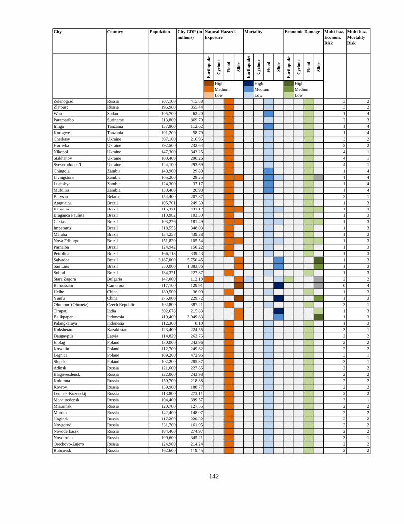
City Country Population City GDP (in
millions)
Multi-haz.
Econom.
Risk
Multi-haz.
Mortality
Risk
Ea
rth
qu
ak
e
Cy
clo
ne
Flo
od
Sli
de
Ea
rth
qu
ak
e
Cy
clo
ne
Flo
od
Sli
de
Ea
rth
qu
ak
e
Cy
clo
ne
Flo
od
Sli
de
3 High 3 High 3 High
2 Medium 2 Medium 2 Medium
1 Low 1 Low 1 Low
Natural Hazards
Exposure
Mortality Economic Damage
Zelenograd Russia 207,100 415.88 0 0 2 0 0 0 1 0 0 0 1 0 3 2
Zlatoust Russia 196,900 355.44 0 0 2 0 0 0 1 0 0 0 1 0 3 2
Wau Sudan 105,700 62.20 0 0 2 0 0 0 2 0 0 0 1 0 1 4
Paramaribo Suriname 213,800 869.70 0 0 2 0 0 0 1 0 0 0 1 0 2 3
Iringa Tanzania 137,900 112.62 0 0 2 0 0 0 2 0 0 0 1 0 1 4
Korogwe Tanzania 101,200 58.79 0 0 2 0 0 0 1 0 0 0 1 0 1 4
Cherkasy Ukraine 307,100 216.95 0 0 2 0 0 0 1 0 0 0 1 0 3 2
Horlivka Ukraine 292,500 232.64 0 0 2 0 0 0 1 0 0 0 1 0 3 2
Nikopol Ukraine 147,300 343.25 0 0 2 0 0 0 1 0 0 0 1 0 4 1
Stakhanov Ukraine 100,400 290.26 0 0 2 0 0 0 1 0 0 0 1 0 4 1
Syeverodonets'k Ukraine 124,100 293.69 0 0 2 0 0 0 1 0 0 0 1 0 4 1
Chingola Zambia 149,900 29.89 0 0 2 0 0 0 2 0 0 0 1 0 1 4
Livingstone Zambia 105,200 28.25 0 0 2 2 0 0 2 1 0 0 1 4 1 4
Luanshya Zambia 124,300 37.17 0 0 2 0 0 0 2 0 0 0 1 0 1 4
Mufulira Zambia 130,400 26.98 0 0 2 0 0 0 2 0 0 0 1 0 1 4
Barysau Belarus 154,400 207.87 0 0 2 0 0 0 1 0 0 0 1 0 3 1
Araguaina Brazil 105,701 249.39 0 0 2 0 0 0 1 0 0 0 1 0 1 3
Barreiras Brazil 115,331 431.12 0 0 2 2 0 0 1 1 0 0 1 1 1 3
Braganca Paulista Brazil 110,982 103.30 0 0 2 0 0 0 1 0 0 0 1 0 1 3
Caxias Brazil 103,276 181.49 0 0 2 2 0 0 1 1 0 0 1 1 1 3
Imperatriz Brazil 218,555 348.03 0 0 2 0 0 0 1 0 0 0 1 0 1 3
Maraba Brazil 134,258 439.38 0 0 2 0 0 0 1 0 0 0 1 0 1 3
Nova Friburgo Brazil 151,820 105.54 0 0 2 2 0 0 1 1 0 0 1 1 1 3
Parnaiba Brazil 124,942 150.22 0 0 2 0 0 0 1 0 0 0 1 0 1 3
Petrolina Brazil 166,113 339.43 0 0 2 0 0 0 1 0 0 0 1 0 1 3
Salvador Brazil 3,187,000 5,750.45 0 0 0 2 0 0 0 2 0 0 0 3 1 3
Sao Luis Brazil 950,000 1,383.86 0 0 0 2 0 0 0 2 0 0 0 2 1 3
Sobral Brazil 134,371 227.87 0 0 2 0 0 0 1 0 0 0 1 0 1 3
Stara Zagora Bulgaria 147,000 112.18 2 0 0 2 1 0 0 1 1 0 0 4 2 2
Bafoussam Cameroon 217,100 129.91 0 0 0 3 0 0 0 3 0 0 0 4 0 4
Heihe China 180,500 36.00 0 0 2 0 0 0 1 0 0 0 1 0 1 3
Yunfu China 275,000 229.72 0 0 0 3 0 0 0 3 0 0 0 2 1 3
Olomouc (Olmuetz) Czech Republic 102,800 387.21 0 0 2 0 0 0 1 0 0 0 1 0 3 1
Tirupati India 302,678 215.83 0 0 0 2 0 0 0 3 0 0 0 1 1 3
Balikpapan Indonesia 419,400 3,049.83 0 0 0 2 0 0 0 2 0 0 0 3 1 3
Palangkaraya Indonesia 112,300 0.10 0 0 2 0 0 0 1 0 0 0 1 0 1 3
Kokshetao Kazakhstan 123,400 224.55 0 0 2 0 0 0 1 0 0 0 1 0 3 1
Daugavpils Latvia 114,829 262.75 0 0 2 0 0 0 1 0 0 0 1 0 2 2
Elblag Poland 130,000 242.96 0 0 2 0 0 0 1 0 0 0 1 0 2 2
Koszalin Poland 112,700 249.82 0 0 2 0 0 0 1 0 0 0 1 0 2 2
Legnica Poland 109,200 472.96 0 0 2 0 0 0 1 0 0 0 1 0 3 1
Slupsk Poland 102,200 285.37 0 0 2 0 0 0 1 0 0 0 1 0 3 1
Adinsk Russia 121,600 227.85 0 0 2 0 0 0 1 0 0 0 1 0 2 2
Blagovesdensk Russia 222,000 243.98 0 0 2 0 0 0 1 0 0 0 1 0 2 2
Kolomna Russia 150,700 218.38 0 0 2 0 0 0 1 0 0 0 1 0 2 2
Kovrov Russia 159,900 188.77 0 0 2 0 0 0 1 0 0 0 1 0 2 2
Leninsk-Kuzneckij Russia 113,800 273.11 0 0 2 0 0 0 1 0 0 0 1 0 2 2
Meaduredensk Russia 104,400 399.57 0 0 2 0 0 0 1 0 0 0 1 0 3 1
Miaurinsk Russia 120,700 127.55 0 0 2 0 0 0 1 0 0 0 1 0 2 2
Murom Russia 142,400 148.07 0 0 2 0 0 0 1 0 0 0 1 0 2 2
Noginsk Russia 117,200 220.32 0 0 2 0 0 0 1 0 0 0 1 0 2 2
Novgorod Russia 231,700 161.95 0 0 2 0 0 0 1 0 0 0 1 0 2 2
Novoderkassk Russia 184,400 274.97 0 0 2 0 0 0 1 0 0 0 1 0 2 2
Novotroick Russia 109,600 345.21 0 0 2 0 0 0 1 0 0 0 1 0 3 1
Orechovo-Zujevo Russia 124,900 214.24 0 0 2 0 0 0 1 0 0 0 1 0 2 2
Rubcovsk Russia 162,600 119.45 0 0 2 0 0 0 1 0 0 0 1 0 2 2
142
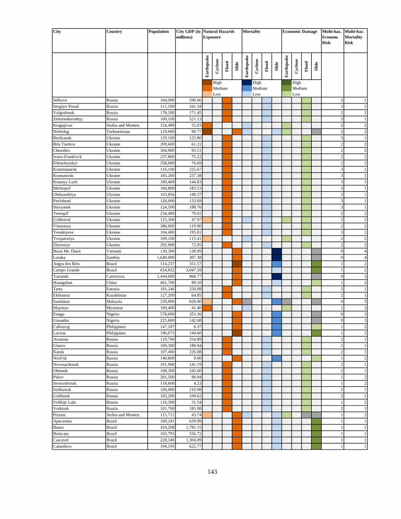
City Country Population City GDP (in
millions)
Multi-haz.
Econom.
Risk
Multi-haz.
Mortality
Risk
Ea
rth
qu
ak
e
Cy
clo
ne
Flo
od
Sli
de
Ea
rth
qu
ak
e
Cy
clo
ne
Flo
od
Sli
de
Ea
rth
qu
ak
e
Cy
clo
ne
Flo
od
Sli
de
3 High 3 High 3 High
2 Medium 2 Medium 2 Medium
1 Low 1 Low 1 Low
Natural Hazards
Exposure
Mortality Economic Damage
Selkovo Russia 104,900 296.66 0 0 2 0 0 0 1 0 0 0 1 0 3 1
Sergijev Posad Russia 111,100 341.34 0 0 2 0 0 0 1 0 0 0 1 0 3 1
Volgodonsk Russia 178,200 171.45 0 0 2 0 0 0 1 0 0 0 1 0 2 2
Zeleznodorodnyj Russia 100,100 521.13 0 0 2 0 0 0 1 0 0 0 1 0 3 1
Kragujevac Serbia and Monten. 154,489 55.03 2 0 0 0 1 0 0 0 1 0 0 0 2 2
Nebitdag Turkmenistan 119,000 90.77 3 0 0 2 1 0 0 1 1 0 0 4 2 2
Berdyansk Ukraine 129,100 125.80 0 0 2 0 0 0 1 0 0 0 1 0 3 1
Bila Tserkva Ukraine 209,600 61.31 0 0 2 0 0 0 1 0 0 0 1 0 2 2
Chernihiv Ukraine 304,900 93.51 0 0 2 0 0 0 1 0 0 0 1 0 2 2
Ivano-Frankivs'k Ukraine 237,800 75.22 0 0 2 0 0 0 1 0 0 0 1 0 2 2
Khmelnytskyi Ukraine 258,000 76.69 0 0 2 0 0 0 1 0 0 0 1 0 2 2
Kommunarsk Ukraine 116,100 225.67 0 0 2 0 0 0 1 0 0 0 1 0 3 1
Kramatorsk Ukraine 183,200 237.38 0 0 2 0 0 0 1 0 0 0 1 0 3 1
Krasnyy Luch Ukraine 100,400 144.83 0 0 2 0 0 0 1 0 0 0 1 0 3 1
Melitopol' Ukraine 166,800 183.53 0 0 2 0 0 0 1 0 0 0 1 0 3 1
Oleksandriya Ukraine 103,856 149.37 0 0 2 0 0 0 1 0 0 0 1 0 3 1
Pavlohrad Ukraine 126,000 133.69 0 0 2 0 0 0 1 0 0 0 1 0 3 1
Slavyansk Ukraine 124,500 188.76 0 0 2 0 0 0 1 0 0 0 1 0 3 1
Ternopil' Ukraine 234,400 79.02 0 0 2 0 0 0 1 0 0 0 1 0 2 2
Uzhhorod Ukraine 125,300 47.97 1 0 2 0 1 0 1 0 1 0 1 0 2 2
Vinnytsya Ukraine 386,000 119.90 0 0 2 0 0 0 1 0 0 0 1 0 2 2
Yenakiyeve Ukraine 104,400 195.81 0 0 2 0 0 0 1 0 0 0 1 0 3 1
Yevpatoriya Ukraine 109,100 115.41 1 0 0 0 1 0 0 0 1 0 0 0 2 2
Zhytomyr Ukraine 292,900 72.95 0 0 2 0 0 0 1 0 0 0 1 0 2 2
Buon Me Thuot Vietnam 130,300 138.09 0 0 0 2 0 0 0 3 0 0 0 4 0 4
Lusaka Zambia 1,640,000 307.38 0 0 0 2 0 0 0 3 0 0 0 4 0 4
Angra dos Reis Brazil 114,237 351.57 0 0 0 3 0 0 0 2 0 0 0 2 1 2
Campo Grande Brazil 654,832 3,047.59 0 0 0 2 0 0 0 1 0 0 0 2 1 2
Yaounde Cameroon 1,444,000 868.77 0 0 0 2 0 0 0 3 0 0 0 4 0 3
Huangshan China 401,700 89.10 0 0 0 2 0 0 0 1 0 0 0 1 1 2
Tartu Estonia 101,246 250.08 0 0 2 0 0 0 1 0 0 0 1 0 2 1
Ekibastuz Kazakhstan 127,200 64.85 0 0 2 0 0 0 1 0 0 0 1 0 2 1
Sandakan Malaysia 220,000 828.90 1 0 0 2 4 0 0 2 4 0 0 4 0 3
Maymyo Myanmar 100,400 41.40 2 0 0 0 1 0 0 0 1 0 0 0 1 2
Enugu Nigeria 578,000 353.36 0 0 0 2 0 0 0 2 0 0 0 4 0 3
Umuahia Nigeria 225,600 142.68 0 0 0 2 0 0 0 2 0 0 0 4 0 3
Calbayog Philippines 147,187 6.37 0 0 0 2 0 0 0 2 0 0 0 1 1 2
Lucena Philippines 196,075 144.60 0 0 0 3 0 0 0 2 0 0 0 2 1 2
Arzamas Russia 110,700 254.89 0 0 2 0 0 0 1 0 0 0 1 0 2 1
Glazov Russia 106,300 188.94 0 0 2 0 0 0 1 0 0 0 1 0 2 1
Kansk Russia 107,400 226.08 0 0 2 0 0 0 1 0 0 0 1 0 2 1
Noril'sk Russia 140,800 0.00 0 0 0 2 0 0 0 2 0 0 0 1 1 2
Novosachtinsk Russia 101,900 141.19 0 0 2 0 0 0 1 0 0 0 1 0 2 1
Obninsk Russia 108,300 245.60 0 0 2 0 0 0 1 0 0 0 1 0 2 1
Pskov Russia 201,500 90.94 0 0 2 0 0 0 1 0 0 0 1 0 1 2
Severodvinsk Russia 118,600 4.23 0 0 2 0 0 0 1 0 0 0 1 0 1 2
Solikamsk Russia 106,000 210.98 0 0 2 0 0 0 1 0 0 0 1 0 2 1
UstIlimsk Russia 105,200 109.62 0 0 2 0 0 0 1 0 0 0 1 0 2 1
Velikije Luki Russia 116,300 31.54 0 0 2 0 0 0 1 0 0 0 1 0 1 2
Votkinsk Russia 101,700 185.98 0 0 2 0 0 0 1 0 0 0 1 0 2 1
Prizren Serbia and Monten. 115,711 43.74 1 0 0 2 1 0 0 1 1 0 4 4 1 2
Apucarana Brazil 100,241 639.99 0 0 0 2 0 0 0 1 0 0 0 2 1 1
Bauru Brazil 310,208 1,781.15 0 0 0 2 0 0 0 1 0 0 0 2 1 1
Botucatu Brazil 103,793 556.72 0 0 0 2 0 0 0 1 0 0 0 2 1 1
Cascavel Brazil 228,340 1,304.09 0 0 0 2 0 0 0 1 0 0 0 2 1 1
Catanduva Brazil 104,195 622.77 0 0 0 2 0 0 0 1 0 0 0 2 1 1
143
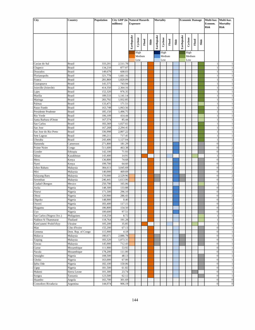
City Country Population City GDP (in
millions)
Multi-haz.
Econom.
Risk
Multi-haz.
Mortality
Risk
Ea
rth
qu
ak
e
Cy
clo
ne
Flo
od
Sli
de
Ea
rth
qu
ak
e
Cy
clo
ne
Flo
od
Sli
de
Ea
rth
qu
ak
e
Cy
clo
ne
Flo
od
Sli
de
3 High 3 High 3 High
2 Medium 2 Medium 2 Medium
1 Low 1 Low 1 Low
Natural Hazards
Exposure
Mortality Economic Damage
Caxias do Sul Brazil 333,201 2,511.78 0 0 0 2 0 0 0 1 0 0 0 2 1 1
Chapeco Brazil 134,210 877.07 0 0 0 2 0 0 0 1 0 0 0 2 1 1
Dourados Brazil 149,679 608.03 0 0 0 2 0 0 0 1 0 0 0 2 1 1
Florianopolis Brazil 321,778 1,661.16 0 0 0 2 0 0 0 1 0 0 0 2 1 1
Franca Brazil 281,869 1,820.09 0 0 0 2 0 0 0 1 0 0 0 2 1 1
Guarapuava Brazil 141,575 743.94 0 0 0 2 0 0 0 1 0 0 0 2 1 1
Joinville (Joinvile) Brazil 414,350 2,364.16 0 0 0 2 0 0 0 1 0 0 0 2 1 1
Lajes Brazil 152,320 976.35 0 0 0 2 0 0 0 1 0 0 0 2 1 1
Marilia Brazil 189,533 1,141.14 0 0 0 2 0 0 0 1 0 0 0 2 1 1
Maringa Brazil 283,792 1,932.85 0 0 0 2 0 0 0 1 0 0 0 2 1 1
Palmas Brazil 133,471 171.51 0 0 0 2 0 0 0 1 0 0 0 1 1 1
Passo Fundo Brazil 163,748 1,063.56 0 0 0 2 0 0 0 1 0 0 0 2 1 1
Presidente Prudente Brazil 185,150 1,496.75 0 0 0 2 0 0 0 1 0 0 0 2 1 1
Rio Verde Brazil 106,109 414.44 0 0 0 2 0 0 0 1 0 0 0 1 1 1
Santa Barbara d'Oeste Brazil 167,574 85.44 0 0 0 2 0 0 0 1 0 0 0 1 1 1
Sao Carlos Brazil 183,369 1,027.02 0 0 0 2 0 0 0 1 0 0 0 2 1 1
Sao Jose Brazil 167,268 2,294.45 0 0 0 2 0 0 0 1 0 0 0 2 1 1
Sao Jose do Rio Preto Brazil 336,998 2,807.22 0 0 0 2 0 0 0 1 0 0 0 2 1 1
Sete Lagoas Brazil 180,211 717.45 0 0 0 2 0 0 0 1 0 0 0 2 1 1
Uberaba Brazil 243,406 1,127.04 0 0 0 2 0 0 0 1 0 0 0 2 1 1
Bamenda Cameroon 271,800 181.29 0 0 0 2 0 0 0 2 0 0 0 4 0 2
Pointe Noire Congo 511,600 463.38 0 0 0 2 0 0 0 2 0 0 0 4 0 2
Gonder Ethiopia 142,100 71.93 0 0 0 2 0 0 0 2 0 0 0 4 0 2
Aktan Kazakhstan 143,400 14.91 0 0 2 0 0 0 1 0 0 0 1 0 1 1
Meru Kenya 136,800 74.68 0 0 0 2 0 0 0 2 0 0 0 4 0 2
Nyeri Kenya 199,700 64.60 0 0 0 2 0 0 0 2 0 0 0 4 0 2
Johor Baharu Malaysia 384,613 3,045.69 0 0 0 2 0 0 0 2 0 0 0 4 0 2
Miri Malaysia 140,000 469.69 0 0 0 2 0 0 0 2 0 0 0 4 0 2
Selayang Baru Malaysia 170,000 2,529.96 1 0 0 2 4 0 0 2 4 0 0 4 0 2
Seremban Malaysia 246,441 1,613.06 1 0 0 2 4 0 0 2 4 0 0 4 0 2
Ciudad Obregon Mexico 250,790 165.06 0 0 0 2 0 0 0 1 0 0 0 1 1 1
Awka Nigeria 148,300 133.88 0 0 0 2 0 0 0 2 0 0 0 4 0 2
Nnewi Nigeria 171,500 296.10 0 0 0 2 0 0 0 2 0 0 0 4 0 2
Obosi Nigeria 120,900 286.43 0 0 0 2 0 0 0 2 0 0 0 4 0 2
Okpoko Nigeria 148,900 0.40 0 0 0 2 0 0 0 2 0 0 0 4 0 2
Owerri Nigeria 183,400 117.15 0 0 0 2 0 0 0 2 0 0 0 4 0 2
Shagamu Nigeria 186,800 154.50 0 0 0 2 0 0 0 1 0 0 0 4 0 2
Uyo Nigeria 100,600 97.51 0 0 0 2 0 0 0 2 0 0 0 4 0 2
San Carlos (Negros Occ.) Philippines 118,259 8.72 0 0 0 2 0 0 0 1 0 0 0 1 1 1
Nakhon Si Thammarat Thailand 118,764 191.28 0 0 0 2 0 0 0 1 0 0 0 1 1 1
Kam'yanets'-Podol's'kyy Ukraine 105,200 35.85 0 0 2 0 0 0 1 0 0 0 1 0 1 1
Man Côte d'Ivoire 155,200 67.13 0 0 0 2 0 0 0 1 0 0 0 4 0 1
Gemena Dem. Rep. of Congo 115,900 4.18 0 0 0 2 0 0 0 1 0 0 0 4 0 1
Malacca Malaysia 180,671 2,886.78 1 0 0 2 4 0 0 1 4 0 0 4 0 1
Taiping Malaysia 183,320 1,073.31 1 0 0 2 4 0 0 1 4 0 0 4 0 1
Tawau Malaysia 145,000 712.43 1 0 0 2 4 0 0 1 4 0 0 4 0 1
Gurue Mozambique 111,900 53.92 0 0 0 2 0 0 0 1 0 0 0 0 0 1
Nacala Mozambique 178,200 111.00 0 0 0 2 0 0 0 1 0 0 0 0 0 1
Amaigbo Nigeria 108,500 48.13 0 0 0 2 0 0 0 1 0 0 0 4 0 1
Gboko Nigeria 163,000 67.00 0 0 0 2 0 0 0 1 0 0 0 4 0 1
Ijebu Ode Nigeria 182,100 150.06 0 0 0 2 0 0 0 1 0 0 0 4 0 1
Ugep Nigeria 181,500 61.82 0 0 0 2 0 0 0 1 0 0 0 4 0 1
Makeni Sierra Leone 101,300 23.74 0 0 0 2 0 0 0 1 0 0 4 0 0 1
Songea Tanzania 123,500 62.12 0 0 0 2 0 0 0 1 0 0 0 4 0 1
Huambo Angola 165,700 301.69 0 0 0 0 0 0 0 0 0 0 0 0 0 0
Comodoro Rivadavia Argentina 144,074 906.19 0 0 0 0 0 0 0 0 0 0 0 0 0 0
144
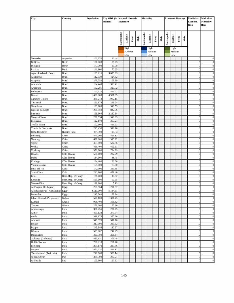
City Country Population City GDP (in
millions)
Multi-haz.
Econom.
Risk
Multi-haz.
Mortality
Risk
Ea
rth
qu
ak
e
Cy
clo
ne
Flo
od
Sli
de
Ea
rth
qu
ak
e
Cy
clo
ne
Flo
od
Sli
de
Ea
rth
qu
ak
e
Cy
clo
ne
Flo
od
Sli
de
3 High 3 High 3 High
2 Medium 2 Medium 2 Medium
1 Low 1 Low 1 Low
Natural Hazards
Exposure
Mortality Economic Damage
Mercedes Argentina 100,876 33.44 0 0 0 0 0 0 0 0 0 0 0 0 0 0
Bohicon Benin 107,200 69.23 0 0 0 0 0 0 0 0 0 0 0 0 0 0
Djougou Benin 177,300 20.38 0 0 0 0 0 0 0 0 0 0 0 0 0 0
Parakou Benin 141,100 72.05 0 0 0 0 0 0 0 0 0 0 0 0 0 0
Aguas Lindas de Goias Brazil 105,216 3,675.63 0 0 0 0 0 0 0 0 0 0 0 0 0 0
Alagoinhas Brazil 112,339 424.62 0 0 0 0 0 0 0 0 0 0 0 0 0 0
Anapolis Brazil 279,752 1,109.69 0 0 0 0 0 0 0 0 0 0 0 0 0 0
Aracatuba Brazil 164,440 1,393.41 0 0 0 0 0 0 0 0 0 0 0 0 0 0
Arapiraca Brazil 152,281 323.72 0 0 0 0 0 0 0 0 0 0 0 0 0 0
Barbacena Brazil 103,522 499.02 0 0 0 0 0 0 0 0 0 0 0 0 0 0
Belem Brazil 1,638,000 4,931.85 0 0 0 0 0 0 0 0 0 0 0 0 0 0
Campina Grande Brazil 336,218 1,002.15 0 0 0 0 0 0 0 0 0 0 0 0 0 0
Castanhal Brazil 121,174 239.24 0 0 0 0 0 0 0 0 0 0 0 0 0 0
Garanhuns Brazil 103,283 340.55 0 0 0 0 0 0 0 0 0 0 0 0 0 0
Juazeiro do Norte Brazil 201,950 842.76 0 0 0 0 0 0 0 0 0 0 0 0 0 0
Luziania Brazil 129,905 2,262.38 0 0 0 0 0 0 0 0 0 0 0 0 0 0
Montes Claros Brazil 288,534 1,340.09 0 0 0 0 0 0 0 0 0 0 0 0 0 0
Paranagua Brazil 122,179 267.24 0 0 0 0 0 0 0 0 0 0 0 0 0 0
Teofilo Otoni Brazil 102,500 455.93 0 0 0 0 0 0 0 0 0 0 0 0 0 0
Vitoria da Conquista Brazil 225,430 910.76 0 0 0 0 0 0 0 0 0 0 0 0 0 0
Bobo Dioulasso Burkina Faso 474,300 128.33 0 0 0 0 0 0 0 0 0 0 0 0 0 0
Baicheng China 471,300 421.13 0 0 0 0 0 0 0 0 0 0 0 0 0 0
Nantong China 639,600 1,393.92 0 0 0 0 0 0 0 0 0 0 0 0 0 0
Siping China 463,000 587.96 0 0 0 0 0 0 0 0 0 0 0 0 0 0
Weihai China 496,400 803.61 0 0 0 0 0 0 0 0 0 0 0 0 0 0
Xuchang China 350,200 784.29 0 0 0 0 0 0 0 0 0 0 0 0 0 0
Bouake Côte d'Ivoire 578,400 232.79 0 0 0 0 0 0 0 0 0 0 0 0 0 0
Daloa Côte d'Ivoire 184,300 88.75 0 0 0 0 0 0 0 0 0 0 0 0 0 0
Korhogo Côte d'Ivoire 164,400 80.36 0 0 0 0 0 0 0 0 0 0 0 0 0 0
Yamoussoukro Côte d'Ivoire 165,000 73.80 0 0 0 0 0 0 0 0 0 0 0 0 0 0
Pinar del Rio Cuba 172,300 333.55 0 0 0 0 0 0 0 0 0 0 0 0 0 0
Santa Clara Cuba 243,900 479.40 0 0 0 0 0 0 0 0 0 0 0 0 0 0
Isiro Dem. Rep. of Congo 131,700 10.92 0 0 0 0 0 0 0 0 0 0 0 0 0 0
Kananga Dem. Rep. of Congo 521,900 53.55 0 0 0 0 0 0 0 0 0 0 0 0 0 0
Mwene-Ditu Dem. Rep. of Congo 189,900 5.13 0 0 0 0 0 0 0 0 0 0 0 0 0 0
Al-Fayyum (El-Fajum) Egypt 260,964 1,291.97 0 0 0 0 0 0 0 0 0 0 0 0 0 0
Al-Iskandariyah (Alexandria) Egypt 4,113,000 5,134.51 0 0 0 0 0 0 0 0 0 0 0 0 0 0
Damanhur Egypt 212,203 179.64 0 0 0 0 0 0 0 0 0 0 0 0 0 0
Libreville (incl. Peripherie) Gabon 526,100 1,331.45 0 0 0 0 0 0 0 0 0 0 0 0 0 0
Kumasi Ghana 906,400 301.82 0 0 0 0 0 0 0 0 0 0 0 0 0 0
Tamale Ghana 259,200 75.20 0 0 0 0 0 0 0 0 0 0 0 0 0 0
Ahmadnagar India 307,455 257.45 0 0 0 0 0 0 0 0 0 0 0 0 0 0
Ajmer India 490,138 270.54 0 0 0 0 0 0 0 0 0 0 0 0 0 0
Akola India 399,978 357.30 0 0 0 0 0 0 0 0 0 0 0 0 0 0
Amravati India 549,370 511.76 0 0 0 0 0 0 0 0 0 0 0 0 0 0
Bellary India 317,000 230.82 0 0 0 0 0 0 0 0 0 0 0 0 0 0
Bijapur India 245,946 182.37 0 0 0 0 0 0 0 0 0 0 0 0 0 0
Bikaner India 529,007 247.29 0 0 0 0 0 0 0 0 0 0 0 0 0 0
Davanagere India 363,780 258.64 0 0 0 0 0 0 0 0 0 0 0 0 0 0
Gulbarga (Gulburga) India 435,631 306.48 0 0 0 0 0 0 0 0 0 0 0 0 0 0
Hubli-Dharwar India 786,018 201.70 0 0 0 0 0 0 0 0 0 0 0 0 0 0
Parbhani India 259,170 233.56 0 0 0 0 0 0 0 0 0 0 0 0 0 0
Solapur India 873,037 589.17 0 0 0 0 0 0 0 0 0 0 0 0 0 0
Thoothukkudi (Tuticorin) India 242,860 308.14 0 0 0 0 0 0 0 0 0 0 0 0 0 0
ad-Diwaniyah Iraq 388,300 207.21 0 0 0 0 0 0 0 0 0 0 0 0 0 0
Al-Kufah Iraq 105,600 120.92 0 0 0 0 0 0 0 0 0 0 0 0 0 0
145

City Country Population City GDP (in
millions)
Multi-haz.
Econom.
Risk
Multi-haz.
Mortality
Risk
Ea
rth
qu
ak
e
Cy
clo
ne
Flo
od
Sli
de
Ea
rth
qu
ak
e
Cy
clo
ne
Flo
od
Sli
de
Ea
rth
qu
ak
e
Cy
clo
ne
Flo
od
Sli
de
3 High 3 High 3 High
2 Medium 2 Medium 2 Medium
1 Low 1 Low 1 Low
Natural Hazards
Exposure
Mortality Economic Damage
As-Samawah Iraq 118,300 0.76 0 0 0 0 0 0 0 0 0 0 0 0 0 0
Machakos Kenya 173,700 59.09 0 0 0 0 0 0 0 0 0 0 0 0 0 0
Antsirabe Madagascar 151,800 10.35 0 0 0 0 0 0 0 0 0 0 0 0 0 0
Fianarantsoa Madagascar 131,600 3.10 0 0 0 0 0 0 0 0 0 0 0 0 0 0
Sikasso Mali 125,400 39.21 0 0 0 0 0 0 0 0 0 0 0 0 0 0
Monclova Mexico 192,554 1,877.68 0 0 0 0 0 0 0 0 0 0 0 0 0 0
San Luis Potosi Mexico 931,000 3,115.06 0 0 0 0 0 0 0 0 0 0 0 0 0 0
Zacatecas Mexico 113,947 419.34 0 0 0 0 0 0 0 0 0 0 0 0 0 0
Agadir Morocco 599,300 437.49 0 0 0 0 0 0 0 0 0 0 0 0 0 0
Beni-Mellal Morocco 153,600 193.05 0 0 0 0 0 0 0 0 0 0 0 0 0 0
Khouribga Morocco 164,600 265.48 0 0 0 0 0 0 0 0 0 0 0 0 0 0
Chimoio Mozambique 192,700 126.30 0 0 0 0 0 0 0 0 0 0 0 0 0 0
Nampula Mozambique 341,700 200.40 0 0 0 0 0 0 0 0 0 0 0 0 0 0
Windhoek Namibia 192,300 662.58 0 0 0 0 0 0 0 0 0 0 0 0 0 0
Agadez Niger 107,000 9.41 0 0 0 0 0 0 0 0 0 0 0 0 0 0
Zinder Niger 195,595 50.43 0 0 0 0 0 0 0 0 0 0 0 0 0 0
Aba Nigeria 766,800 273.56 0 0 0 0 0 0 0 0 0 0 0 0 0 0
Abuja Nigeria 154,200 43.70 0 0 0 0 0 0 0 0 0 0 0 0 0 0
Ado Nigeria 235,600 138.96 0 0 0 0 0 0 0 0 0 0 0 0 0 0
Akure Nigeria 361,200 198.68 0 0 0 0 0 0 0 0 0 0 0 0 0 0
Bugama Nigeria 119,700 67.73 0 0 0 0 0 0 0 0 0 0 0 0 0 0
Damaturu Nigeria 218,000 47.07 0 0 0 0 0 0 0 0 0 0 0 0 0 0
Efon Alaye Nigeria 239,900 45.06 0 0 0 0 0 0 0 0 0 0 0 0 0 0
Ejigbo Nigeria 114,100 64.57 0 0 0 0 0 0 0 0 0 0 0 0 0 0
Funtua Nigeria 119,500 65.37 0 0 0 0 0 0 0 0 0 0 0 0 0 0
Gbongan Nigeria 115,000 76.97 0 0 0 0 0 0 0 0 0 0 0 0 0 0
Gombe Nigeria 224,600 99.04 0 0 0 0 0 0 0 0 0 0 0 0 0 0
Ibadan Nigeria 1,731,000 2,045.19 0 0 0 0 0 0 0 0 0 0 0 0 0 0
Ife Nigeria 307,300 168.94 0 0 0 0 0 0 0 0 0 0 0 0 0 0
Igboho Nigeria 112,800 75.40 0 0 0 0 0 0 0 0 0 0 0 0 0 0
Ijero Nigeria 143,900 66.66 0 0 0 0 0 0 0 0 0 0 0 0 0 0
Ikare Nigeria 156,800 70.21 0 0 0 0 0 0 0 0 0 0 0 0 0 0
Ikire Nigeria 183,300 83.77 0 0 0 0 0 0 0 0 0 0 0 0 0 0
Ikirun Nigeria 125,900 77.59 0 0 0 0 0 0 0 0 0 0 0 0 0 0
Ikot Ekpene Nigeria 205,700 144.18 0 0 0 0 0 0 0 0 0 0 0 0 0 0
Ila Nigeria 147,800 64.20 0 0 0 0 0 0 0 0 0 0 0 0 0 0
Ilawe Nigeria 157,000 88.11 0 0 0 0 0 0 0 0 0 0 0 0 0 0
Ilesha Nigeria 229,300 0.19 0 0 0 0 0 0 0 0 0 0 0 0 0 0
Ilorin Nigeria 732,700 436.23 0 0 0 0 0 0 0 0 0 0 0 0 0 0
Inisa Nigeria 135,400 45.88 0 0 0 0 0 0 0 0 0 0 0 0 0 0
Ise Nigeria 163,200 70.40 0 0 0 0 0 0 0 0 0 0 0 0 0 0
Iseyin Nigeria 281,100 137.48 0 0 0 0 0 0 0 0 0 0 0 0 0 0
Jalingo Nigeria 101,200 2.57 0 0 0 0 0 0 0 0 0 0 0 0 0 0
Kishi Nigeria 128,200 101.64 0 0 0 0 0 0 0 0 0 0 0 0 0 0
Lafia Nigeria 112,500 61.27 0 0 0 0 0 0 0 0 0 0 0 0 0 0
Offa Nigeria 102,300 63.27 0 0 0 0 0 0 0 0 0 0 0 0 0 0
Ogbomosho Nigeria 712,100 245.56 0 0 0 0 0 0 0 0 0 0 0 0 0 0
Okene Nigeria 430,900 371.36 0 0 0 0 0 0 0 0 0 0 0 0 0 0
Okrika Nigeria 117,800 88.17 0 0 0 0 0 0 0 0 0 0 0 0 0 0
Ondo Nigeria 220,600 122.55 0 0 0 0 0 0 0 0 0 0 0 0 0 0
Owo Nigeria 237,400 113.94 0 0 0 0 0 0 0 0 0 0 0 0 0 0
Oyo Nigeria 608,300 310.46 0 0 0 0 0 0 0 0 0 0 0 0 0 0
Port Harcourt Nigeria 1,016,200 73.73 0 0 0 0 0 0 0 0 0 0 0 0 0 0
Shaki Nigeria 147,300 90.35 0 0 0 0 0 0 0 0 0 0 0 0 0 0
Suleja Nigeria 145,500 38.20 0 0 0 0 0 0 0 0 0 0 0 0 0 0
Warri Nigeria 486,700 11.59 0 0 0 0 0 0 0 0 0 0 0 0 0 0
146

City Country Population City GDP (in
millions)
Multi-haz.
Econom.
Risk
Multi-haz.
Mortality
Risk
Ea
rth
qu
ak
e
Cy
clo
ne
Flo
od
Sli
de
Ea
rth
qu
ak
e
Cy
clo
ne
Flo
od
Sli
de
Ea
rth
qu
ak
e
Cy
clo
ne
Flo
od
Sli
de
3 High 3 High 3 High
2 Medium 2 Medium 2 Medium
1 Low 1 Low 1 Low
Natural Hazards
Exposure
Mortality Economic Damage
Khanpur Pakistan 117,764 87.94 0 0 0 0 0 0 0 0 0 0 0 0 0 0
Waldenburg Poland 135,700 471.67 0 0 0 0 0 0 0 0 0 0 0 0 0 0
Zielona Gora (Gruenberg) Poland 118,800 410.15 0 0 0 0 0 0 0 0 0 0 0 0 0 0
Elista Russia 103,300 72.67 0 0 0 0 0 0 0 0 0 0 0 0 0 0
Kolpino Russia 141,200 618.44 0 0 0 0 0 0 0 0 0 0 0 0 0 0
Leningrad Russia 5,133,000 3,756.63 0 0 0 0 0 0 0 0 0 0 0 0 0 0
Murmansk Russia 376,300 1,390.32 0 0 0 0 0 0 0 0 0 0 0 0 0 0
Sachty Russia 221,800 381.93 0 0 0 0 0 0 0 0 0 0 0 0 0 0
Salavat Russia 156,800 347.96 0 0 0 0 0 0 0 0 0 0 0 0 0 0
Vologda Russia 302,500 994.71 0 0 0 0 0 0 0 0 0 0 0 0 0 0
Mbour Senegal 122,400 32.44 0 0 0 0 0 0 0 0 0 0 0 0 0 0
Thies Senegal 255,200 84.79 0 0 0 0 0 0 0 0 0 0 0 0 0 0
Koidu Sierra Leone 109,900 2.90 0 0 0 0 0 0 0 0 0 0 0 0 0 0
Singapore Singapore 3,567,000 80,516.77 0 0 0 0 0 0 0 0 0 0 0 0 0 0
Hargeisa Somalia 197,100 44.01 0 0 0 0 0 0 0 0 0 0 0 0 0 0
Merca Somalia 168,200 5.75 0 0 0 0 0 0 0 0 0 0 0 0 0 0
Benoni South Africa 399,400 2,076.47 0 0 0 0 0 0 0 0 0 0 0 0 0 0
Bloemfontein South Africa 364,700 1,640.85 0 0 0 0 0 0 0 0 0 0 0 0 0 0
Boksburg South Africa 285,100 1,675.58 0 0 0 0 0 0 0 0 0 0 0 0 0 0
Brakpan South Africa 187,300 1,348.13 0 0 0 0 0 0 0 0 0 0 0 0 0 0
George South Africa 102,900 534.61 0 0 0 0 0 0 0 0 0 0 0 0 0 0
Johannesburg South Africa 2,335,000 9,219.15 0 0 0 0 0 0 0 0 0 0 0 0 0 0
Kimberley South Africa 186,200 853.92 0 0 0 0 0 0 0 0 0 0 0 0 0 0
King Williams Town South Africa 101,900 718.65 0 0 0 0 0 0 0 0 0 0 0 0 0 0
Krugersdorp South Africa 222,000 2,866.14 0 0 0 0 0 0 0 0 0 0 0 0 0 0
Randfontein South Africa 107,100 2,205.04 0 0 0 0 0 0 0 0 0 0 0 0 0 0
Springs South Africa 175,700 710.67 0 0 0 0 0 0 0 0 0 0 0 0 0 0
Tembisa South Africa 308,500 2,906.26 0 0 0 0 0 0 0 0 0 0 0 0 0 0
Westonaria South Africa 124,500 1,481.80 0 0 0 0 0 0 0 0 0 0 0 0 0 0
Al-Fasir Sudan 178,500 56.67 0 0 0 0 0 0 0 0 0 0 0 0 0 0
Al-Junaynah Sudan 116,800 83.31 0 0 0 0 0 0 0 0 0 0 0 0 0 0
Al-Qadarif Sudan 240,500 249.07 0 0 0 0 0 0 0 0 0 0 0 0 0 0
Al-Ubayyid Sudan 288,600 105.72 0 0 0 0 0 0 0 0 0 0 0 0 0 0
Bur Sudan Sudan 384,100 0.00 0 0 0 0 0 0 0 0 0 0 0 0 0 0
Dodoma Tanzania 159,100 102.25 0 0 0 0 0 0 0 0 0 0 0 0 0 0
Sfax Tunisia 257,800 420.12 0 0 0 0 0 0 0 0 0 0 0 0 0 0
Play Cu Vietnam 102,000 35.51 0 0 0 0 0 0 0 0 0 0 0 0 0 0
Ndola Zambia 568,600 72.08 0 0 0 0 0 0 0 0 0 0 0 0 0 0
Bulawayo Zimbabwe 794,600 123.03 0 0 0 0 0 0 0 0 0 0 0 0 0 0
Gweru Zimbabwe 163,900 36.64 0 0 0 0 0 0 0 0 0 0 0 0 0 0
Mutare Zimbabwe 168,100 139.91 0 0 0 0 0 0 0 0 0 0 0 0 0 0
147

148
APPENDIX 2: COPYRIGHT PERMISSIONS
1. Permission from Westermann
----- Original Message -----
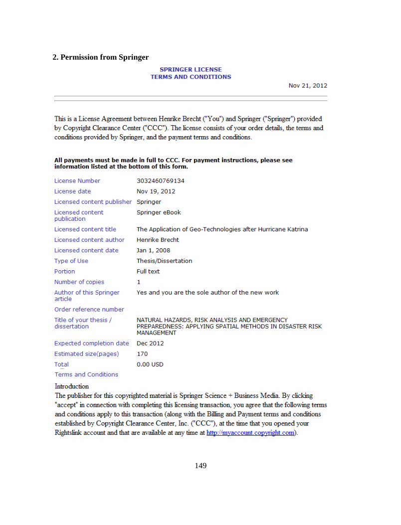
149
2. Permission from Springer

150
151

152

153
3. Permission from SAGE
154
155
VITA
Henrike Brecht was born in Bad Gandersheim, Germany. She was awarded a M.S. in
Environmental Science from Westfaelische Wilhelms-University in Muenster, Germany, in
2002. During her M.S. studies, she was a research assistant at the Institute for
Geoinformatics in Muenster. After graduation, Henrike worked for the United Nations High
Commissioner for Refugees (UNHCR) in Switzerland, Kenya and Sudan. In 2004, she
started her doctoral studies at Louisiana State University (LSU) in Geography and
Anthropology under the advisorship of Dr. Michael Leitner and with financing from the
Economic Development Scholarship through the LSU Hurricane Center. In 2007, she took a
position as a Disaster Risk Management Specialist at the World Bank, where she has
enjoyed implementing risk reduction projects predominantly in Southeast Asian countries.
She expects to receive her Doctor of Philosophy degree in December 2012.