natural language processing machine learning tools zhao hai 赵海 department of computer science...
TRANSCRIPT
Natural Language Processing
machine learning tools
Zhao Hai 赵海
Department of Computer Science and Engineering
Shanghai Jiao Tong University
2
Machine Learning Approaches for Natural Language Processing
k-Nearest Neighbor
Support Vector Machine
Maximum Entropy (log-linear) Model
Outline
3
What’s Machine Learning
• Learning from some known data, and give predictions on unknown data.
• Typically, classification.• Types
– Supervised learning: labeled data are necessary– Unsupervised learning: only unlabeled data are used
but some heuristic rules are necessary.– Semi-supervised learning: both labeled and unlabeled
data are used.
4
What’s Machine Learning
• What we are talking about is supervised machine learning.
• Natural language processing often asks for structure learning.
5
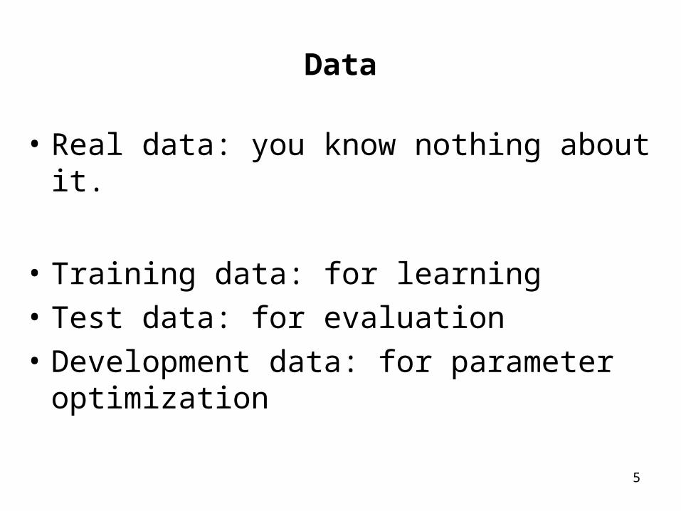
Data
• Real data: you know nothing about it.
• Training data: for learning
• Test data: for evaluation
• Development data: for parameter optimization
6
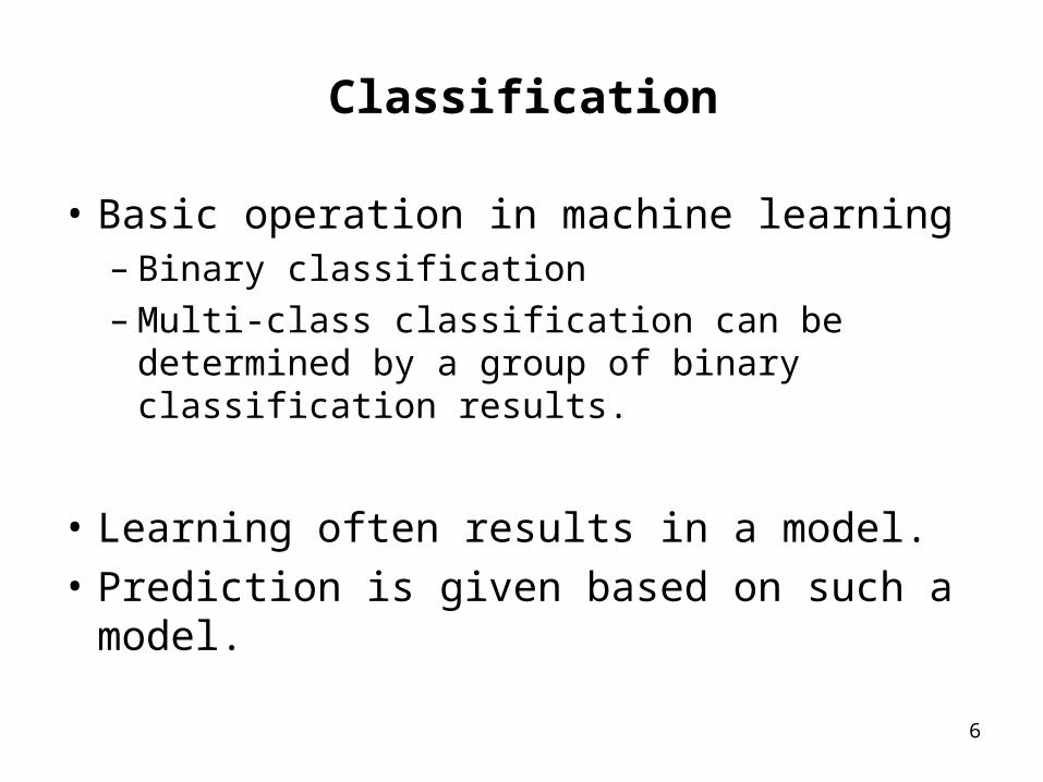
Classification
• Basic operation in machine learning– Binary classification– Multi-class classification can be determined
by a group of binary classification results.
• Learning often results in a model.
• Prediction is given based on such a model.
7
Machine Learning Approaches for Natural Language Processing
k-Nearest Neighbor
Support Vector Machine
Maximum Entropy (log-linear) Model
Outline
k-Nearest Neighbor (k-NN)
This part is based on slides by Xia Fei

9
Instance-based (IB) learning
• No training: store all training instances. “Lazy learning”
• Examples:– k-NN– Locally weighted regression– Radial basis functions– Case-based reasoning– …
• The most well-known IB method: k-NN

10
k-NN
+
+
+
+
+
++ +
o
o
o o
o
o
oo
o
o
o
oo
o
o
o
o
o?
11
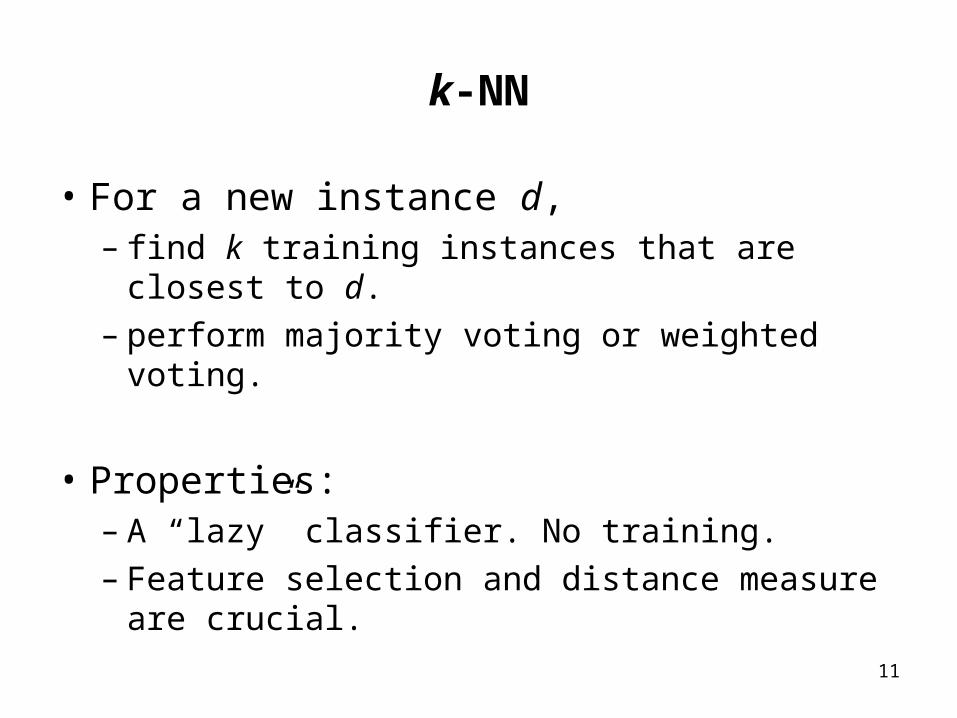
k-NN
• For a new instance d,– find k training instances that are closest to d.– perform majority voting or weighted voting.
• Properties:– A “lazy” classifier. No training.– Feature selection and distance measure are
crucial.
12
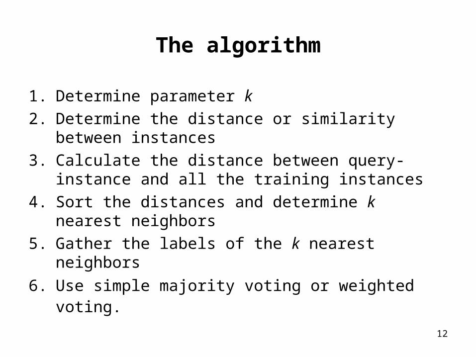
The algorithm
1. Determine parameter k
2. Determine the distance or similarity between instances
3. Calculate the distance between query-instance and all the training instances
4. Sort the distances and determine k nearest neighbors
5. Gather the labels of the k nearest neighbors
6. Use simple majority voting or weighted voting.
13
Picking k
• Use N-fold cross validation: pick the one that minimizes cross validation error.
14
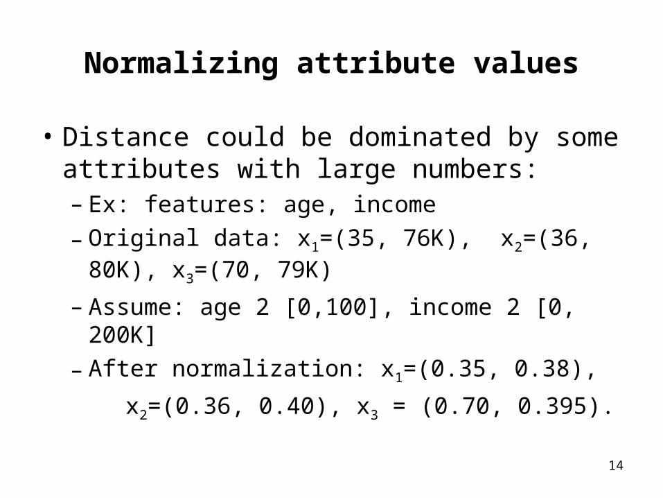
Normalizing attribute values
• Distance could be dominated by some attributes with large numbers:– Ex: features: age, income
– Original data: x1=(35, 76K), x2=(36, 80K), x3=(70, 79K)
– Assume: age 2 [0,100], income 2 [0, 200K]
– After normalization: x1=(0.35, 0.38),
x2=(0.36, 0.40), x3 = (0.70, 0.395).
15
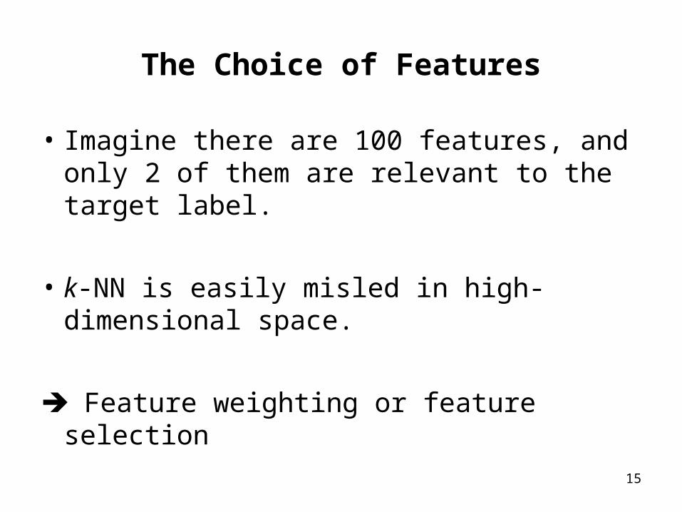
The Choice of Features
• Imagine there are 100 features, and only 2 of them are relevant to the target label.
• k-NN is easily misled in high-dimensional space.
Feature weighting or feature selection
16
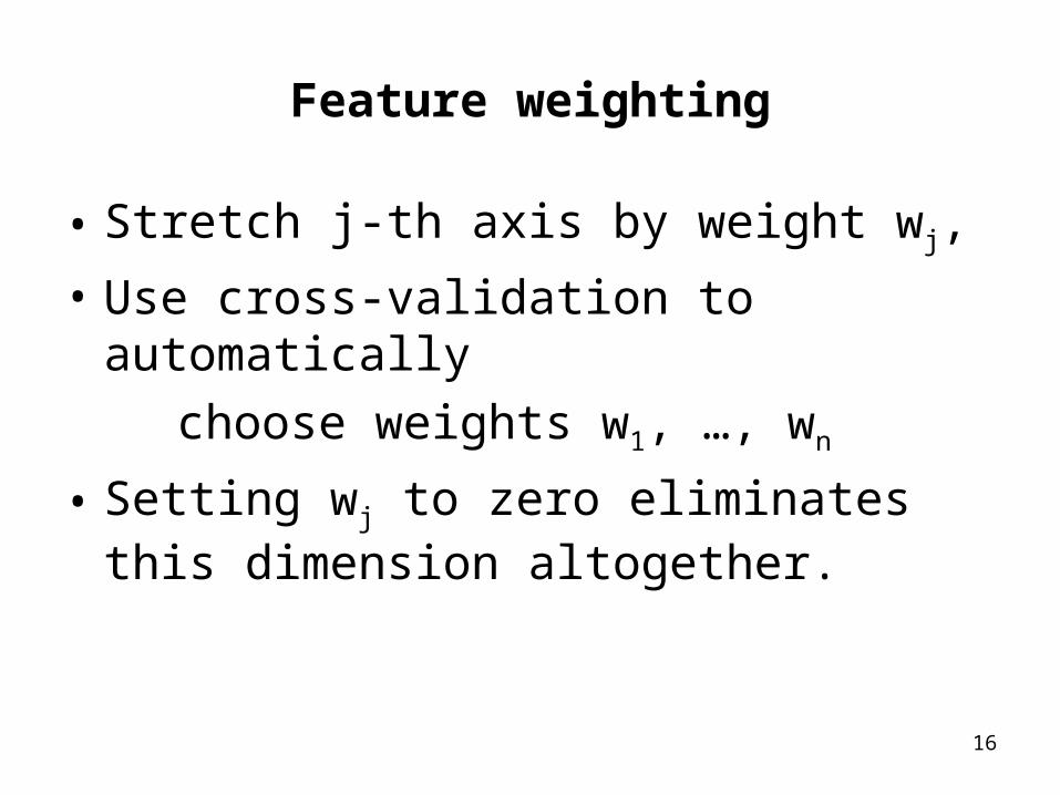
Feature weighting
• Stretch j-th axis by weight wj,
• Use cross-validation to automatically
choose weights w1, …, wn
• Setting wj to zero eliminates this dimension altogether.
17
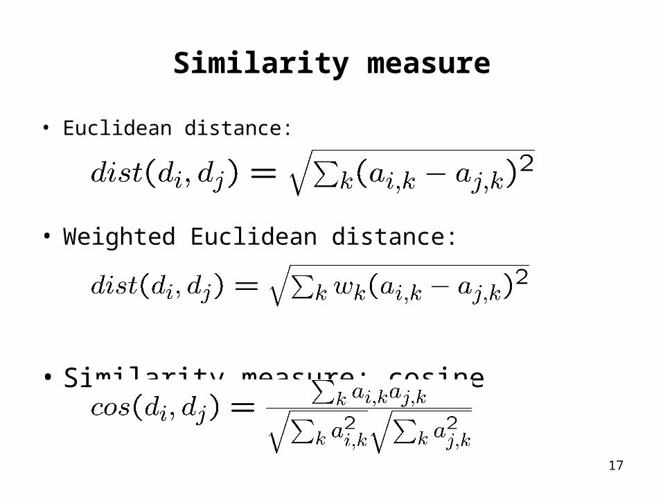
Similarity measure
• Euclidean distance:
• Weighted Euclidean distance:
• Similarity measure: cosine
18
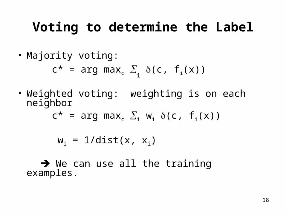
Voting to determine the Label
• Majority voting:
c* = arg maxc i (c, fi(x))
• Weighted voting: weighting is on each neighbor c* = arg maxc i wi (c, fi(x))
wi = 1/dist(x, xi)
We can use all the training examples.
19
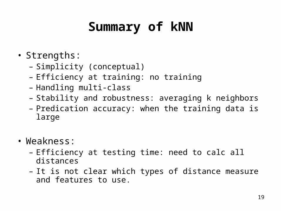
Summary of kNN
• Strengths:– Simplicity (conceptual)– Efficiency at training: no training– Handling multi-class– Stability and robustness: averaging k neighbors– Predication accuracy: when the training data is large
• Weakness:– Efficiency at testing time: need to calc all distances– It is not clear which types of distance measure and
features to use.
20
Machine Learning Approaches for Natural Language Processing
k-Nearest Neighbor
Support Vector Machine
Maximum Entropy (log-linear) Model
Outline
Support Vector Machines
This part is partially revised from the slides byConstantin F. Aliferis & Loannis Tsamardinos
22
Support Vector Machines
• Decision surface is a hyperplane (line in 2D) in feature space (similar to the Perceptron)
• Arguably, the most important recent discovery in machine learning
• In a nutshell: – Find the hyperplane that maximizes the margin
between the two classes– If data are not separable find the hyperplane that
maximizes the margin and minimizes the (a weighted average of the) misclassifications
– map the data to a predetermined very high-dimensional space via a kernel function
23
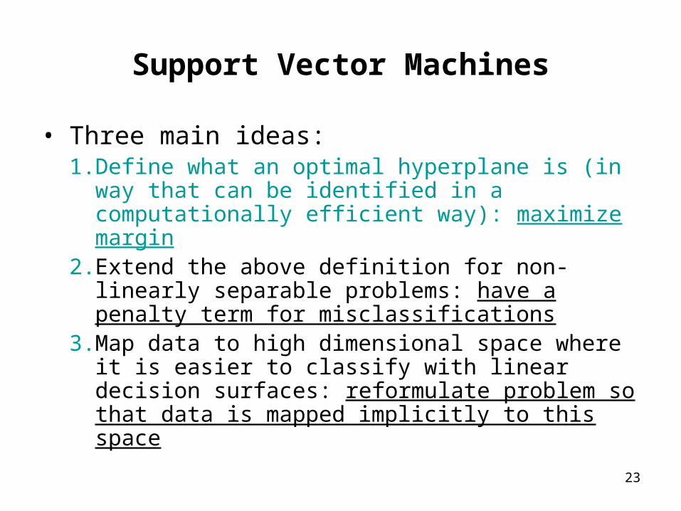
Support Vector Machines
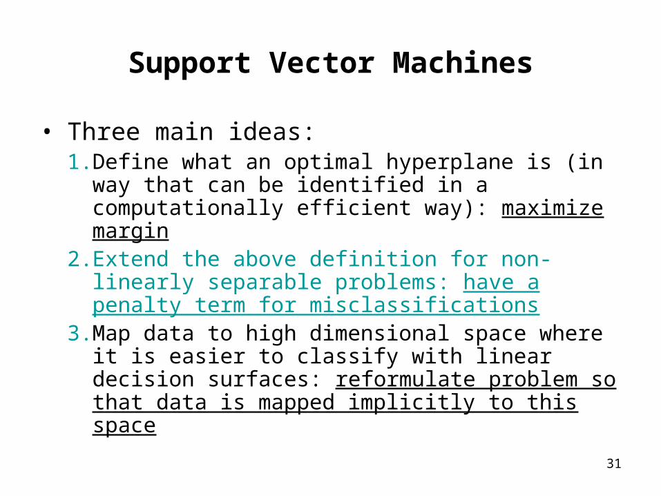
• Three main ideas:1. Define what an optimal hyperplane is (in way
that can be identified in a computationally efficient way): maximize margin
2. Extend the above definition for non-linearly separable problems: have a penalty term for misclassifications
3. Map data to high dimensional space where it is easier to classify with linear decision surfaces: reformulate problem so that data is mapped implicitly to this space
24
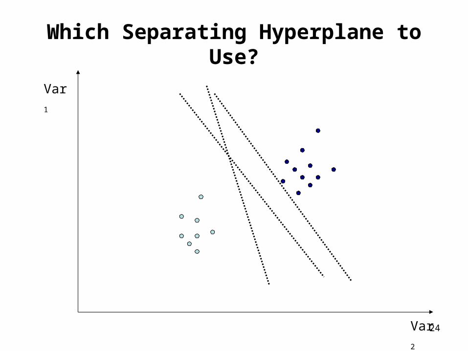
Which Separating Hyperplane to Use?
Var1
Var2
25
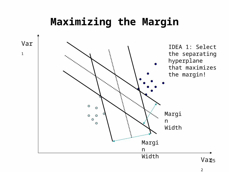
Maximizing the Margin
Var1
Var2
Margin Width
Margin Width
IDEA 1: Select the separating hyperplane that maximizes the margin!
26
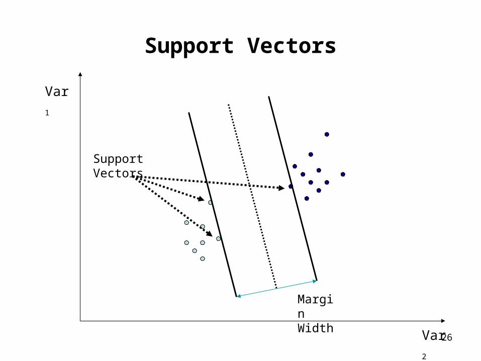
Support Vectors
Var1
Var2
Margin Width
Support Vectors
27
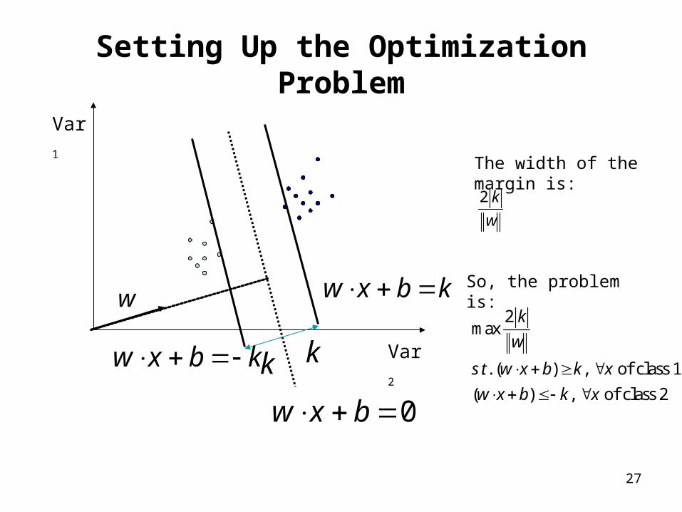
Setting Up the Optimization Problem
Var1
Var2kbxw
kbxw
0 bxwkk
w
The width of the margin is:
2 k
w
So, the problem is:
2max
. . ( ) , of class 1
( ) , of class 2
k
w
s t w x b k x
w x b k x
28
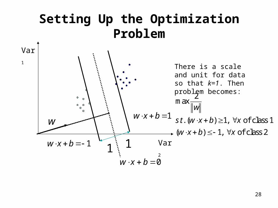
Setting Up the Optimization Problem
Var1
Var21w x b
1w x b
0 bxw
11
w
There is a scale and unit for data so that k=1. Then problem becomes:
2max
. . ( ) 1, of class 1
( ) 1, of class 2
w
s t w x b x
w x b x
29
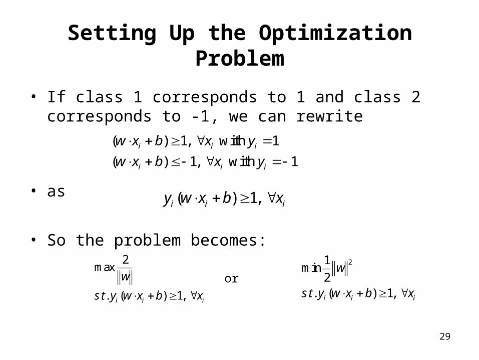
Setting Up the Optimization Problem
• If class 1 corresponds to 1 and class 2 corresponds to -1, we can rewrite
• as
• So the problem becomes:
( ) 1, with 1
( ) 1, with 1i i i
i i i
w x b x y
w x b x y
( ) 1, i i iy w x b x
2max
. . ( ) 1, i i i
w
s t y w x b x
21min
2. . ( ) 1, i i i
w
s t y w x b x or
30
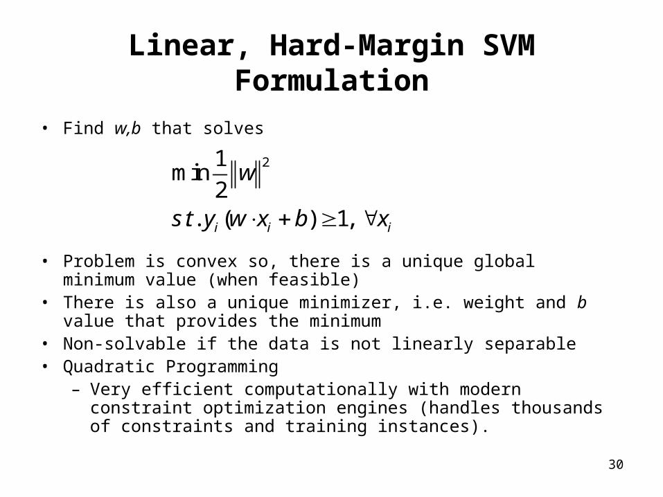
Linear, Hard-Margin SVM Formulation
• Find w,b that solves
• Problem is convex so, there is a unique global minimum value (when feasible)
• There is also a unique minimizer, i.e. weight and b value that provides the minimum
• Non-solvable if the data is not linearly separable• Quadratic Programming
– Very efficient computationally with modern constraint optimization engines (handles thousands of constraints and training instances).
21min
2. . ( ) 1, i i i
w
s t y w x b x
31
Support Vector Machines
• Three main ideas:1. Define what an optimal hyperplane is (in way
that can be identified in a computationally efficient way): maximize margin
2. Extend the above definition for non-linearly separable problems: have a penalty term for misclassifications
3. Map data to high dimensional space where it is easier to classify with linear decision surfaces: reformulate problem so that data is mapped implicitly to this space
32
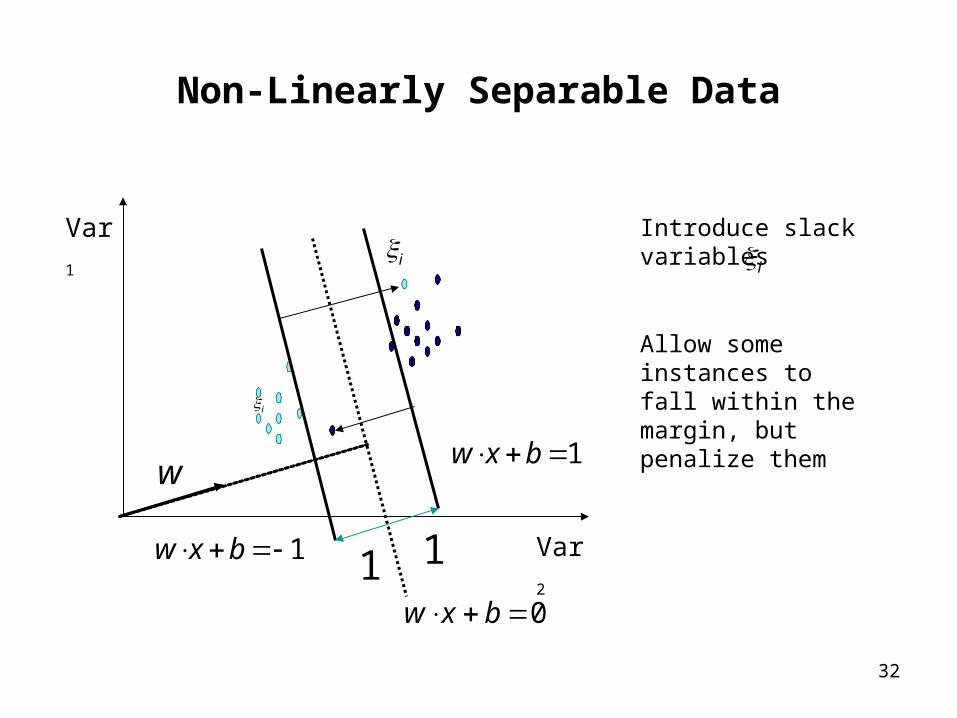
Non-Linearly Separable Data
i
Var1
Var21w x b
1w x b
0 bxw
11
w
iIntroduce slack variables
Allow some instances to fall within the margin, but penalize them
i
33
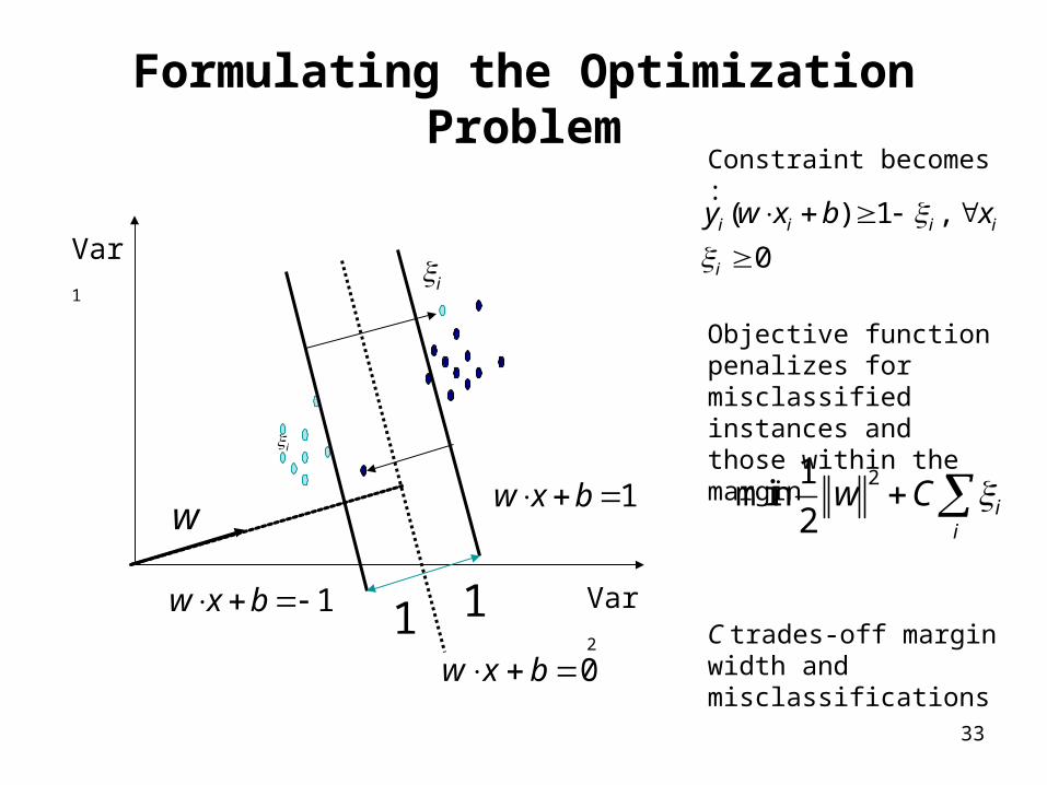
Formulating the Optimization Problem
i
Var1
Var21w x b
1w x b
0 bxw
11
w
i
Constraint becomes :
Objective function penalizes for misclassified instances and those within the margin
C trades-off margin width and misclassifications
( ) 1 ,
0i i i i
i
y w x b x
21min
2 ii
w C
34
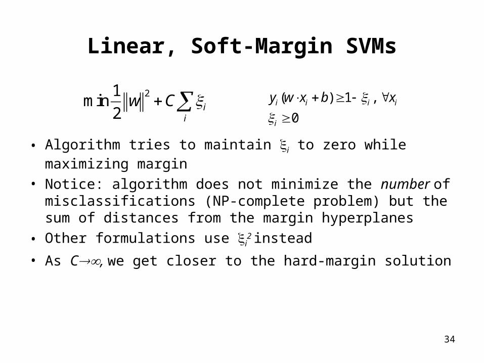
Linear, Soft-Margin SVMs
• Algorithm tries to maintain i to zero while maximizing margin
• Notice: algorithm does not minimize the number of misclassifications (NP-complete problem) but the sum of distances from the margin hyperplanes
• Other formulations use i2 instead
• As C, we get closer to the hard-margin solution
( ) 1 ,
0i i i i
i
y w x b x
21min
2 ii
w C
35
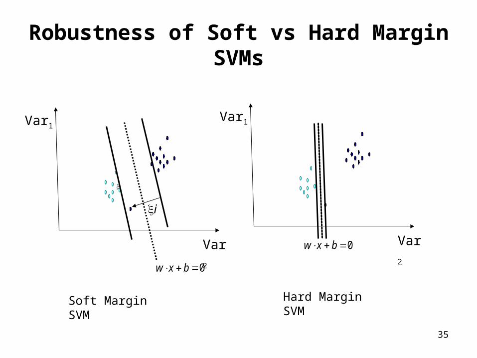
Robustness of Soft vs Hard Margin SVMs
i
Var1
Var2
0 bxw
i
Var1
Var20 bxw
Soft Margin SVM Hard Margin SVM
36
Soft vs Hard Margin SVM
• Soft-Margin SVMs always have a solution• Soft-Margin is more robust to outliers
– Smoother surfaces (in the non-linear case)• Hard-Margin does not require to guess the cost
parameter (requires no parameters at all)
37
Support Vector Machines
• Three main ideas:1. Define what an optimal hyperplane is (in way
that can be identified in a computationally efficient way): maximize margin
2. Extend the above definition for non-linearly separable problems: have a penalty term for misclassifications
3. Map data to high dimensional space where it is easier to classify with linear decision surfaces: reformulate problem so that data is mapped implicitly to this space
38
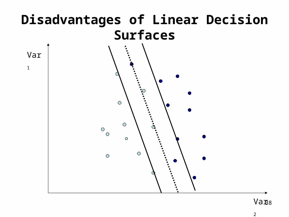
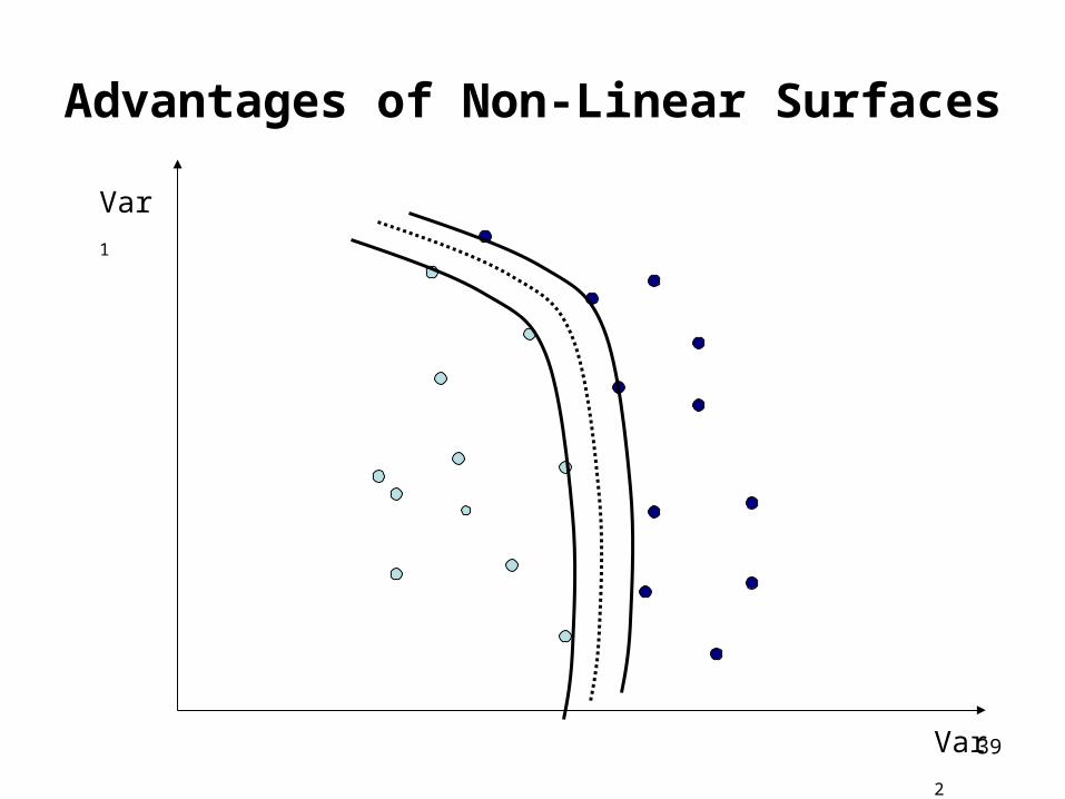
Disadvantages of Linear Decision Surfaces
Var1
Var2
39
Advantages of Non-Linear Surfaces
Var1
Var2
40
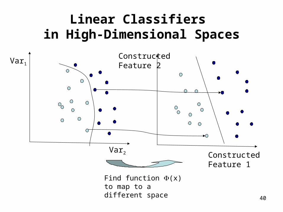
Linear Classifiers in High-Dimensional Spaces
Var1
Var2 Constructed Feature 1
Find function (x) to map to a different space
Constructed Feature 2
41
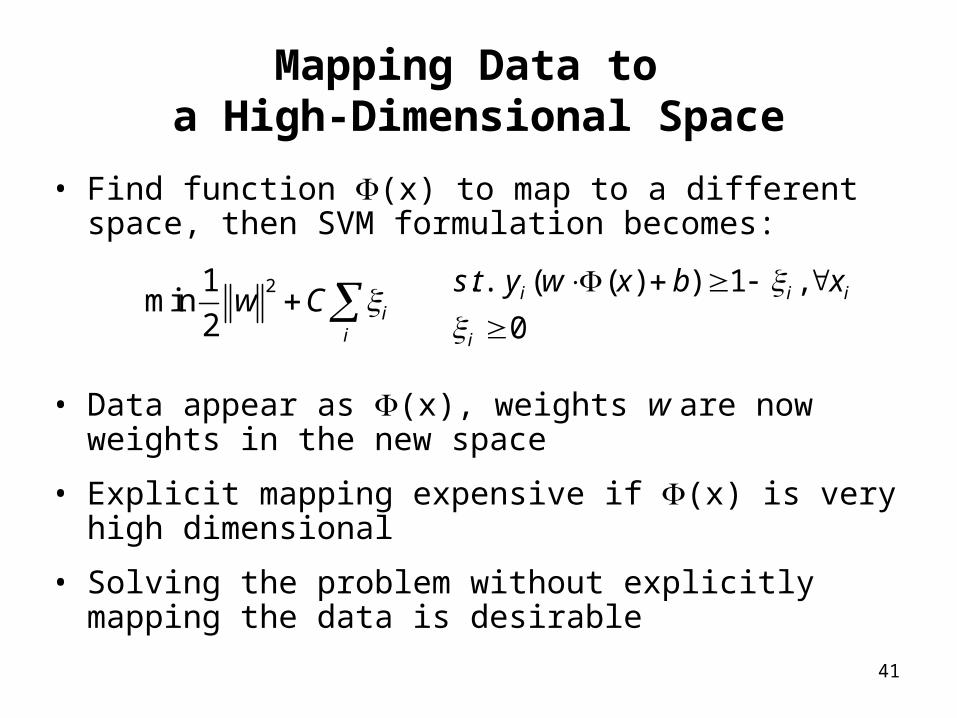
Mapping Data to a High-Dimensional Space
• Find function (x) to map to a different space, then SVM formulation becomes:
• Data appear as (x), weights w are now weights in the new space
• Explicit mapping expensive if (x) is very high dimensional
• Solving the problem without explicitly mapping the data is desirable
21min
2 ii
w C 0
,1))(( ..
i
iii xbxwyts
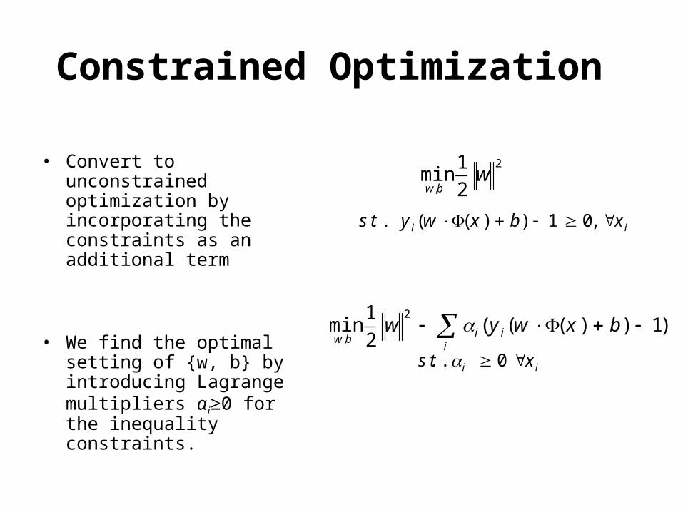
Constrained Optimization
• Convert to unconstrained optimization by incorporating the constraints as an additional term
• We find the optimal setting of {w, b} by introducing Lagrange multipliers αi≥0 for the inequality constraints.
ii xbxwyts ,01))(( ..
2
, 21
min wbw
ii xts 0 ..
i
iibwbxwyw )1))(((
21
min2
,
Constrained Optimization
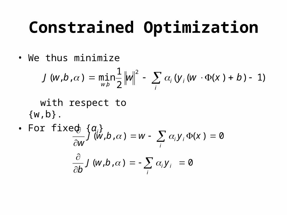
• We thus minimize
with respect to {w,b}.
• For fixed {αi}
i
iibwbxwywbwJ )1))(((
21
min),,(2
,
0),,(
0)(),,(
iii
iii
ybwJb
xywbwJw
44
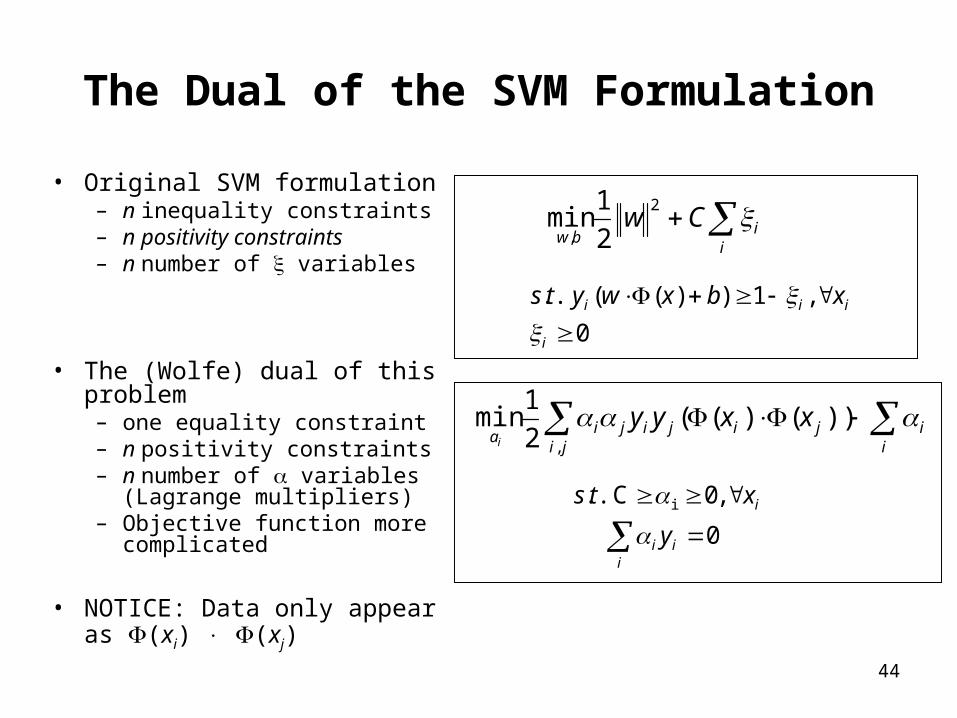
The Dual of the SVM Formulation
• Original SVM formulation– n inequality constraints– n positivity constraints– n number of variables
• The (Wolfe) dual of this problem– one equality constraint– n positivity constraints– n number of variables
(Lagrange multipliers)– Objective function more
complicated
• NOTICE: Data only appear as (xi) (xj)
0
,1))(( ..
i
iii xbxwyts
i
ibw
Cw 2
, 2
1min
iii
i
y
xts
0
,0C .. i
ji i
ijijijia
xxyyi ,
))()((2
1min
45
The Kernel Trick
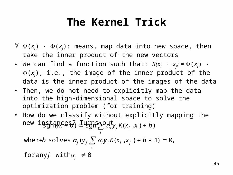
(xi) (xj): means, map data into new space, then take the inner product of the new vectors
• We can find a function such that: K(xi xj) = (xi) (xj), i.e., the image of the inner product of the data is the inner product of the images of the data
• Then, we do not need to explicitly map the data into the high-dimensional space to solve the optimization problem (for training)
• How do we classify without explicitly mapping the new instances? Turns out
0 with any for
,0)1),(( solves where
)),(sgn()sgn(
j
ijiiijj
iiii
j
bxxKyyb
bxxKybwx
46
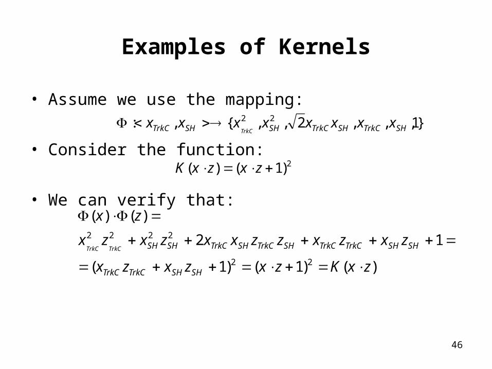
Examples of Kernels
• Assume we use the mapping:
• Consider the function:
• We can verify that:
}1,,,2,,{,: 22SHTrkCSHTrkCSHSHTrkC xxxxxxxx
TrkC
2)1()( zxzxK
)()1()1(
12
)()(
22
2222
zxKzxzxzx
zxzxzzxxzxzx
zx
SHSHTrkCTrkC
SHSHTrkCTrkCSHTrkCSHTrkCSHSHTrkCTrkC
47
Polynomial and Gaussian Kernels
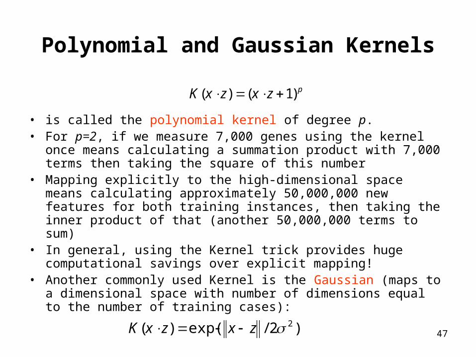
• is called the polynomial kernel of degree p.• For p=2, if we measure 7,000 genes using the kernel once means
calculating a summation product with 7,000 terms then taking the square of this number
• Mapping explicitly to the high-dimensional space means calculating approximately 50,000,000 new features for both training instances, then taking the inner product of that (another 50,000,000 terms to sum)
• In general, using the Kernel trick provides huge computational savings over explicit mapping!
• Another commonly used Kernel is the Gaussian (maps to a dimensional space with number of dimensions equal to the number of training cases):
pzxzxK )1()(
)2/exp()( 2zxzxK
48
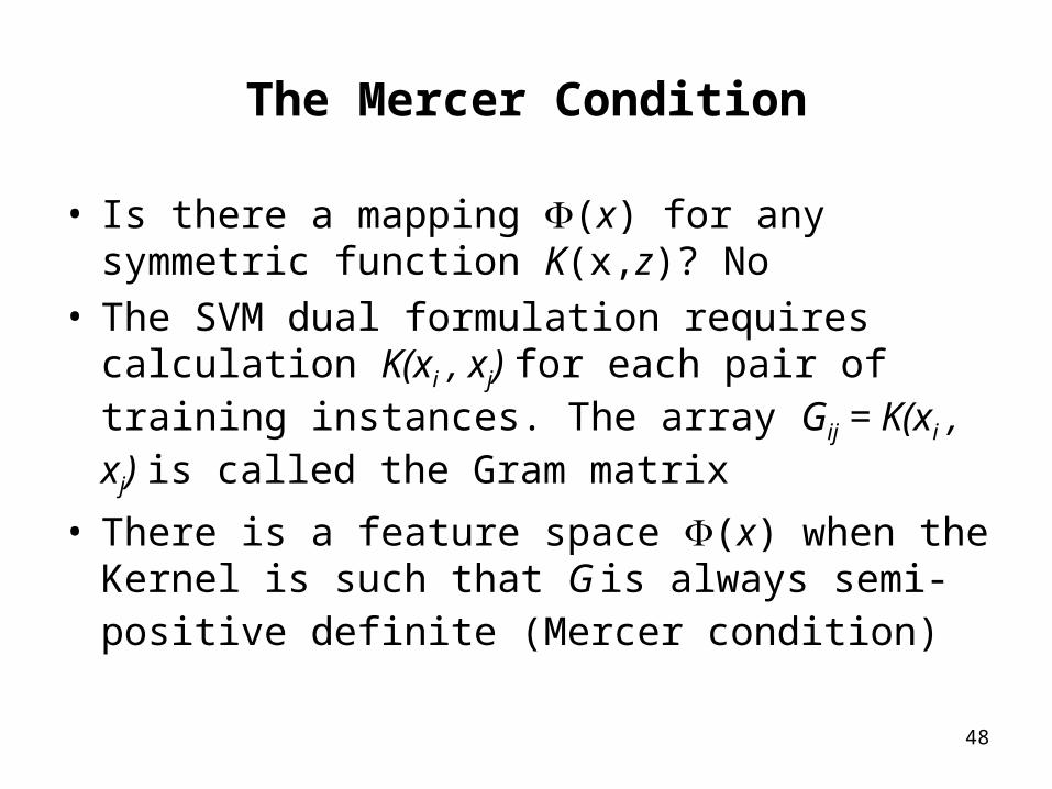
The Mercer Condition
• Is there a mapping (x) for any symmetric function K(x,z)? No
• The SVM dual formulation requires calculation K(xi , xj) for each pair of training instances. The array Gij = K(xi , xj) is called the Gram matrix
• There is a feature space (x) when the Kernel is such that G is always semi-positive definite (Mercer condition)
49
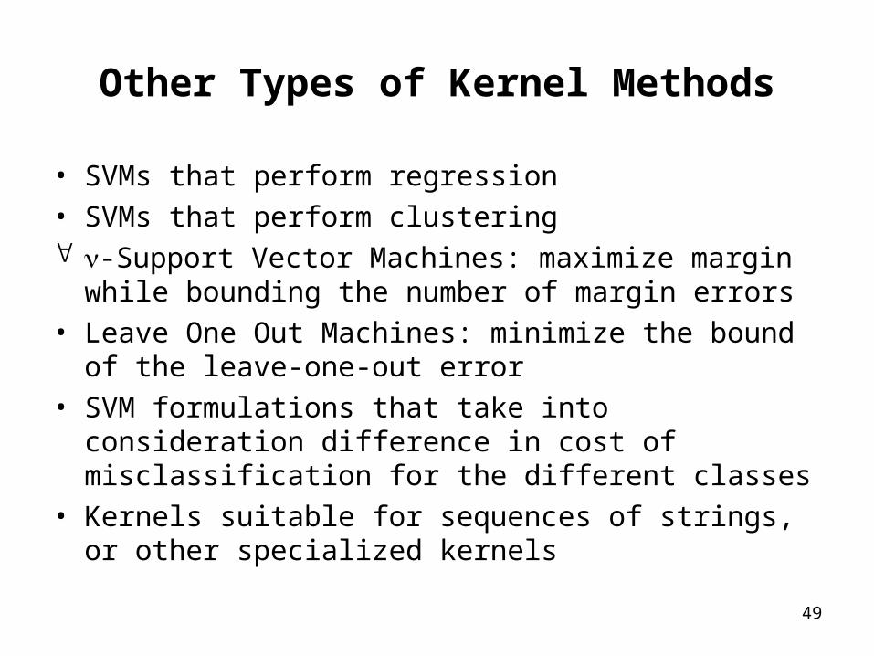
Other Types of Kernel Methods
• SVMs that perform regression• SVMs that perform clustering -Support Vector Machines: maximize margin while
bounding the number of margin errors• Leave One Out Machines: minimize the bound of the
leave-one-out error• SVM formulations that take into consideration difference
in cost of misclassification for the different classes• Kernels suitable for sequences of strings, or other
specialized kernels
50
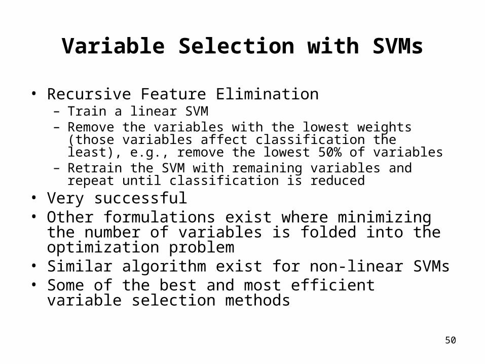
Variable Selection with SVMs
• Recursive Feature Elimination– Train a linear SVM– Remove the variables with the lowest weights (those variables
affect classification the least), e.g., remove the lowest 50% of variables
– Retrain the SVM with remaining variables and repeat until classification is reduced
• Very successful• Other formulations exist where minimizing the number of
variables is folded into the optimization problem• Similar algorithm exist for non-linear SVMs• Some of the best and most efficient variable selection
methods
51
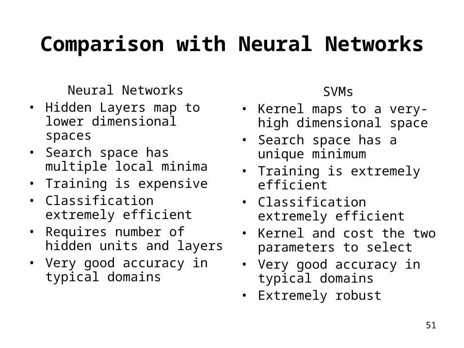
Comparison with Neural Networks
Neural Networks• Hidden Layers map to lower
dimensional spaces• Search space has multiple
local minima• Training is expensive• Classification extremely
efficient• Requires number of hidden
units and layers• Very good accuracy in typical
domains
SVMs• Kernel maps to a very-high
dimensional space• Search space has a unique
minimum• Training is extremely efficient• Classification extremely
efficient• Kernel and cost the two
parameters to select• Very good accuracy in typical
domains• Extremely robust
52
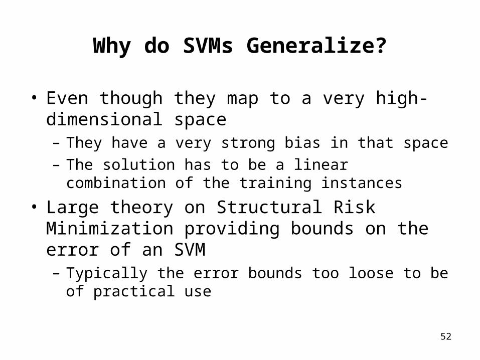
Why do SVMs Generalize?
• Even though they map to a very high-dimensional space– They have a very strong bias in that space– The solution has to be a linear combination of the
training instances
• Large theory on Structural Risk Minimization providing bounds on the error of an SVM– Typically the error bounds too loose to be of practical
use
53
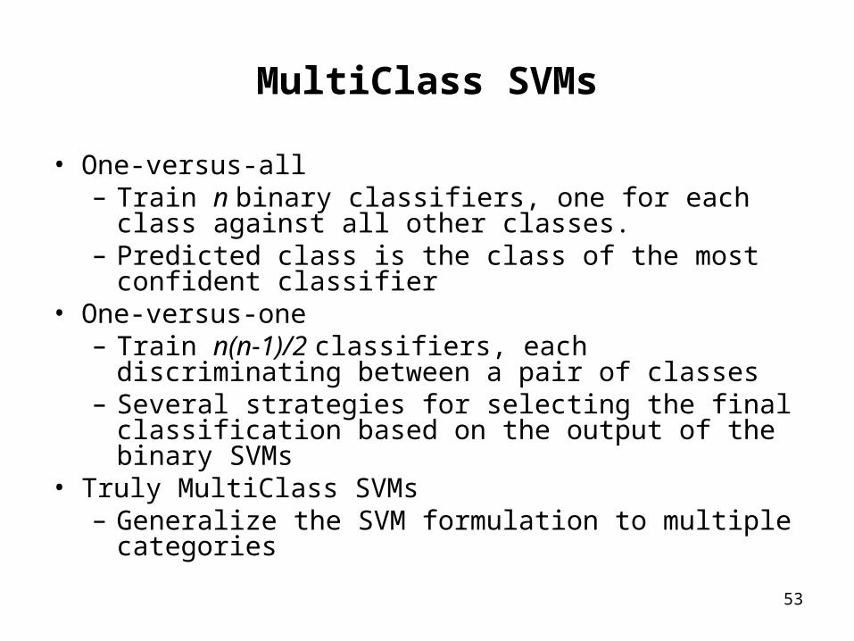
MultiClass SVMs
• One-versus-all– Train n binary classifiers, one for each class against
all other classes.– Predicted class is the class of the most confident
classifier• One-versus-one
– Train n(n-1)/2 classifiers, each discriminating between a pair of classes
– Several strategies for selecting the final classification based on the output of the binary SVMs
• Truly MultiClass SVMs– Generalize the SVM formulation to multiple categories
54
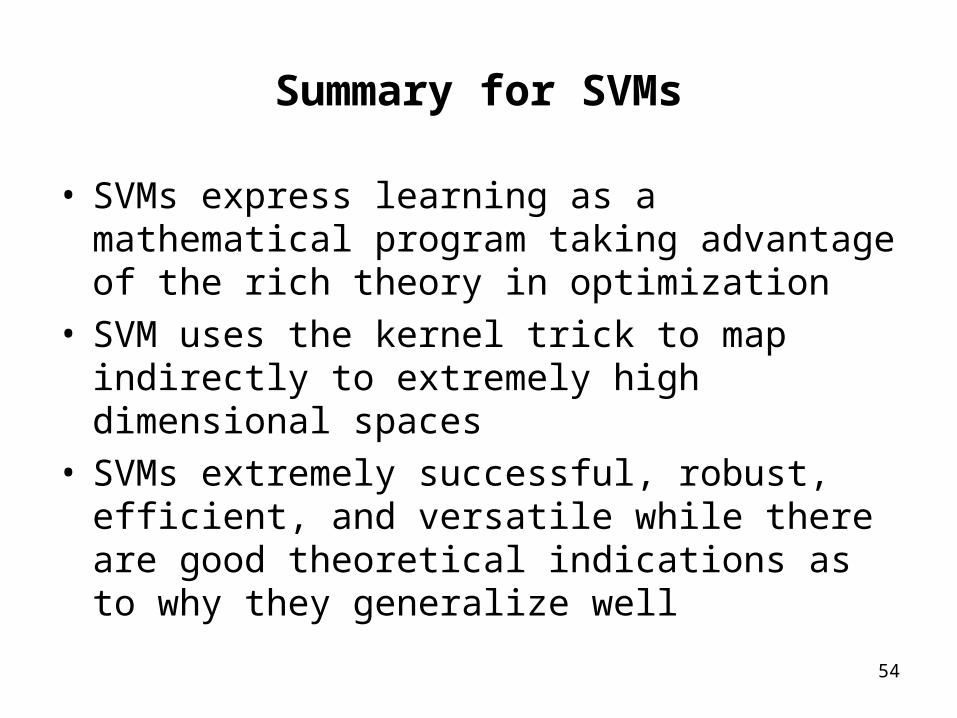
Summary for SVMs
• SVMs express learning as a mathematical program taking advantage of the rich theory in optimization
• SVM uses the kernel trick to map indirectly to extremely high dimensional spaces
• SVMs extremely successful, robust, efficient, and versatile while there are good theoretical indications as to why they generalize well
55
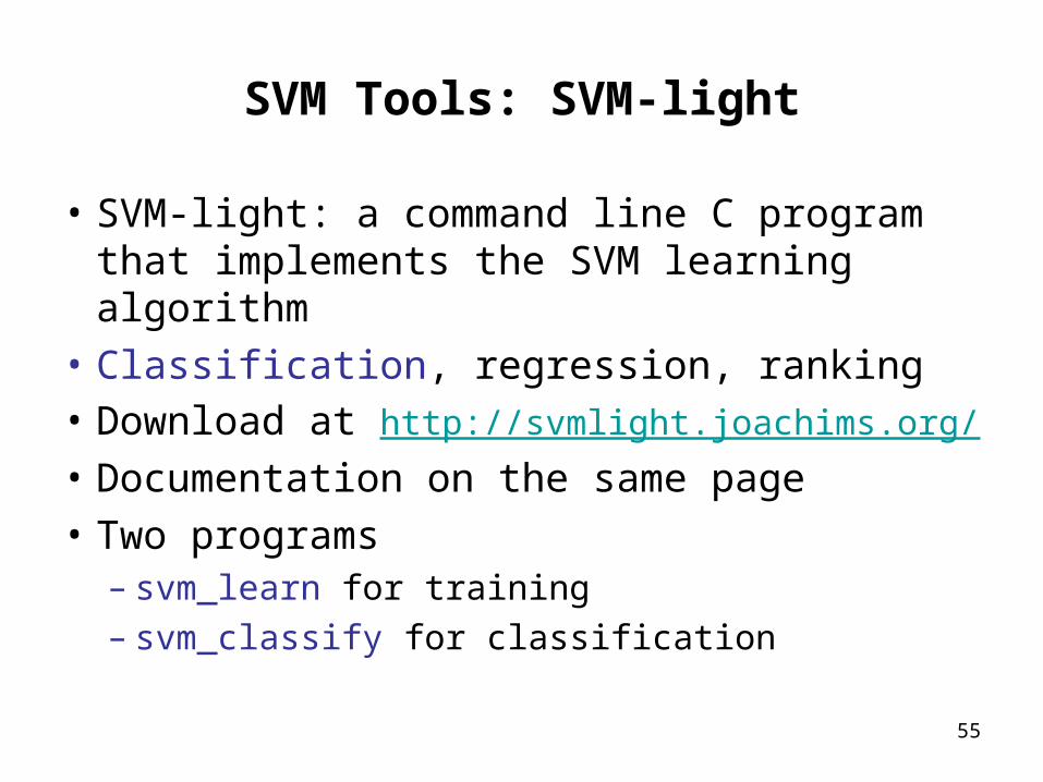
SVM Tools: SVM-light
• SVM-light: a command line C program that implements the SVM learning algorithm
• Classification, regression, ranking• Download at http://svmlight.joachims.org/
• Documentation on the same page
• Two programs– svm_learn for training– svm_classify for classification
56
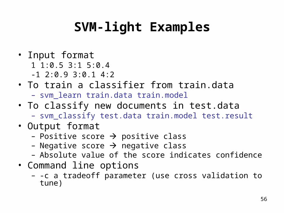
SVM-light Examples
• Input format1 1:0.5 3:1 5:0.4-1 2:0.9 3:0.1 4:2
• To train a classifier from train.data– svm_learn train.data train.model
• To classify new documents in test.data– svm_classify test.data train.model test.result
• Output format– Positive score positive class– Negative score negative class– Absolute value of the score indicates confidence
• Command line options– -c a tradeoff parameter (use cross validation to tune)
57
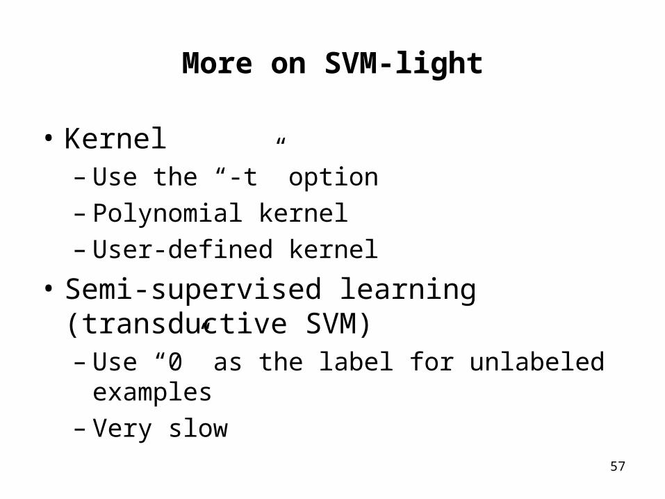
More on SVM-light
• Kernel– Use the “-t” option– Polynomial kernel– User-defined kernel
• Semi-supervised learning (transductive SVM)– Use “0” as the label for unlabeled examples– Very slow
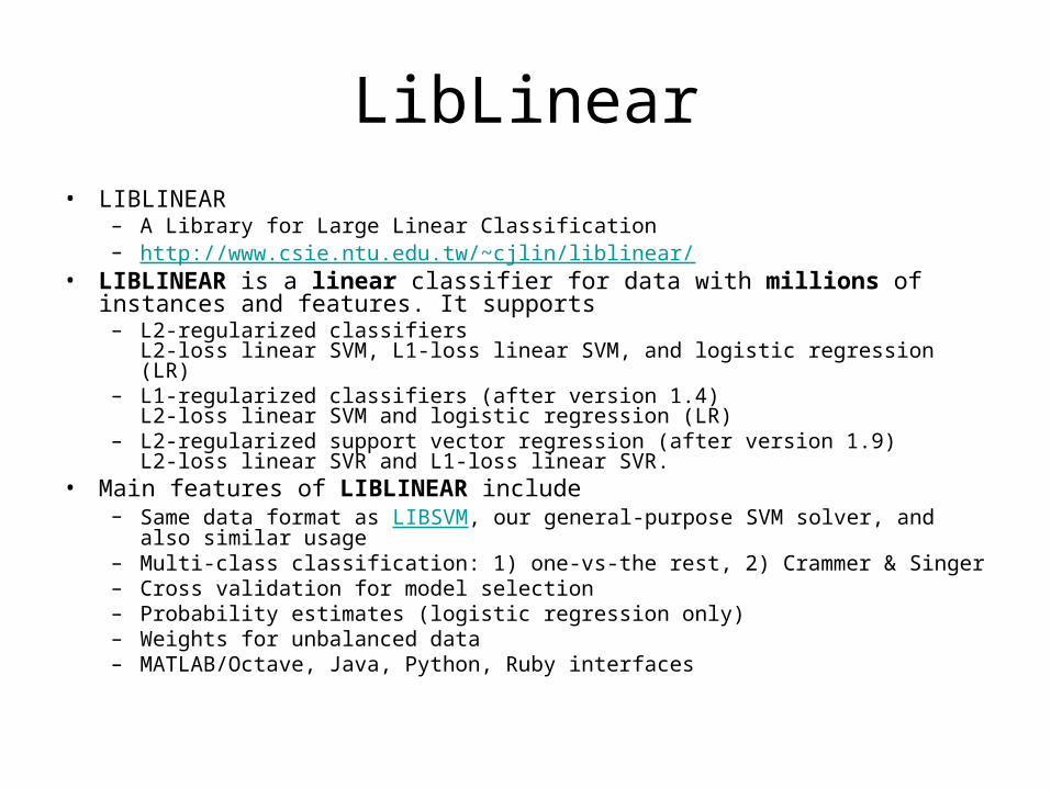
LibLinear• LIBLINEAR
– A Library for Large Linear Classification – http://www.csie.ntu.edu.tw/~cjlin/liblinear/
• LIBLINEAR is a linear classifier for data with millions of instances and features. It supports
– L2-regularized classifiers L2-loss linear SVM, L1-loss linear SVM, and logistic regression (LR)
– L1-regularized classifiers (after version 1.4) L2-loss linear SVM and logistic regression (LR)
– L2-regularized support vector regression (after version 1.9) L2-loss linear SVR and L1-loss linear SVR.
• Main features of LIBLINEAR include – Same data format as LIBSVM, our general-purpose SVM solver, and also similar
usage – Multi-class classification: 1) one-vs-the rest, 2) Crammer & Singer – Cross validation for model selection – Probability estimates (logistic regression only) – Weights for unbalanced data – MATLAB/Octave, Java, Python, Ruby interfaces
59
Machine Learning Approaches for Natural Language Processing k-Nearest Neighbor
Support Vector Machine
Maximum Entropy (log-linear) Model
(this part is revised from that by Michael Collins)
Outline
60
Overview
• Log-linear models
• The maximum-entropy property
• Smoothing, feature selection etc. in log-linear models
61
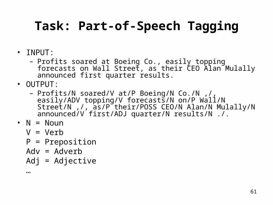
Task: Part-of-Speech Tagging
• INPUT:– Profits soared at Boeing Co., easily topping forecasts on Wall
Street, as their CEO Alan Mulally announced first quarter results.• OUTPUT:
– Profits/N soared/V at/P Boeing/N Co./N ,/, easily/ADV topping/V forecasts/N on/P Wall/N Street/N ,/, as/P their/POSS CEO/N Alan/N Mulally/N announced/V first/ADJ quarter/N results/N ./.
• N = NounV = VerbP = PrepositionAdv = AdverbAdj = Adjective…
62
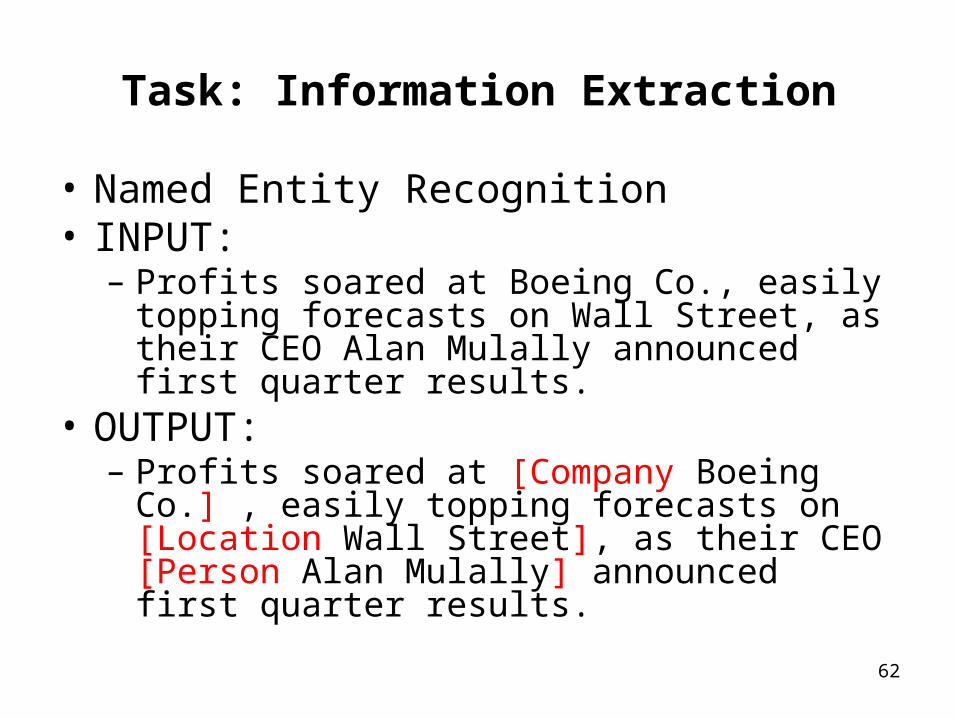
Task: Information Extraction
• Named Entity Recognition• INPUT:
– Profits soared at Boeing Co., easily topping forecasts on Wall Street, as their CEO Alan Mulally announced first quarter results.
• OUTPUT:– Profits soared at [Company Boeing Co.] , easily
topping forecasts on [Location Wall Street], as their CEO [Person Alan Mulally] announced first quarter results.
63
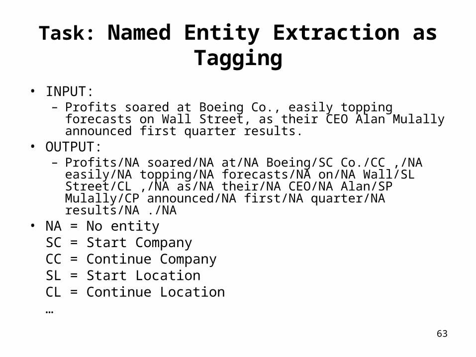
Task: Named Entity Extraction as Tagging
• INPUT: – Profits soared at Boeing Co., easily topping forecasts on Wall
Street, as their CEO Alan Mulally announced first quarter results.• OUTPUT:
– Profits/NA soared/NA at/NA Boeing/SC Co./CC ,/NA easily/NA topping/NA forecasts/NA on/NA Wall/SL Street/CL ,/NA as/NA their/NA CEO/NA Alan/SP Mulally/CP announced/NA first/NA quarter/NA results/NA ./NA
• NA = No entitySC = Start CompanyCC = Continue CompanySL = Start LocationCL = Continue Location…
64
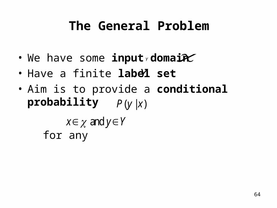
The General Problem
• We have some input domain• Have a finite label set • Aim is to provide a conditional probability
for any
Y
Y
( | )P y x
and x y Y
65
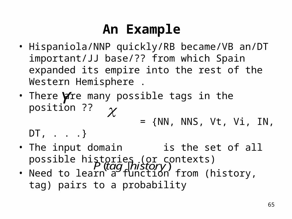
An Example• Hispaniola/NNP quickly/RB became/VB an/DT
important/JJ base/?? from which Spain expanded its empire into the rest of the Western Hemisphere .
• There are many possible tags in the position ??
= {NN, NNS, Vt, Vi, IN, DT, . . .}• The input domain is the set of all possible histories (or
contexts)• Need to learn a function from (history, tag) pairs to a
probability
Y
( | )P tag history

66
Representation: Histories
• A history is a 4-tuple• are the previous two tags.• are the n words in the input sentence. • is the index of the word being tagged• is the set of all possible histories • Hispaniola/NNP quickly/RB became/VB an/DT
important/JJ base/?? from which Spain expanded its empire into the rest of the Western Hemisphere .– = DT, JJ
– = <Hispaniola, quickly, became,…, Hemisphere, .>
– = 6
1 2 [1: ], , ,nt t w i
1 2,t t
w
[1: ]nw
i
1 2,t t
[1: ]nwi
67
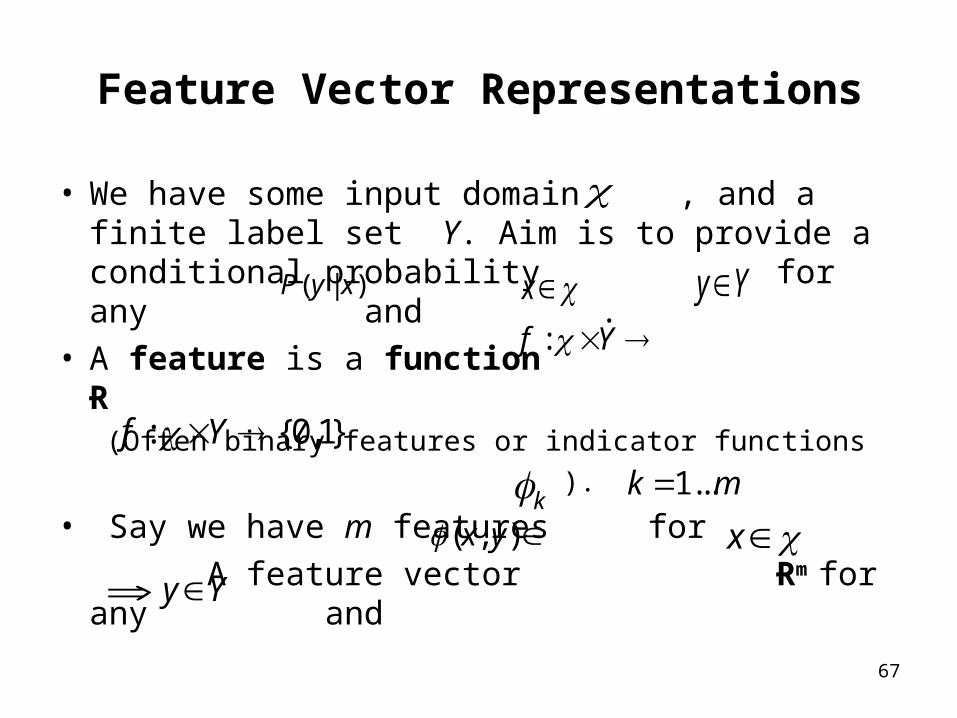
Feature Vector Representations
• We have some input domain , and a finite label set Y. Aim is to provide a conditional probability for any and .
• A feature is a function Ɍ (Often binary features or indicator functions
).
• Say we have m features for
A feature vector Ɍm for any and
( | )P y x x y Y:f Y
: {0,1}f Y
k 1...k m
( , )x y x y Y
68
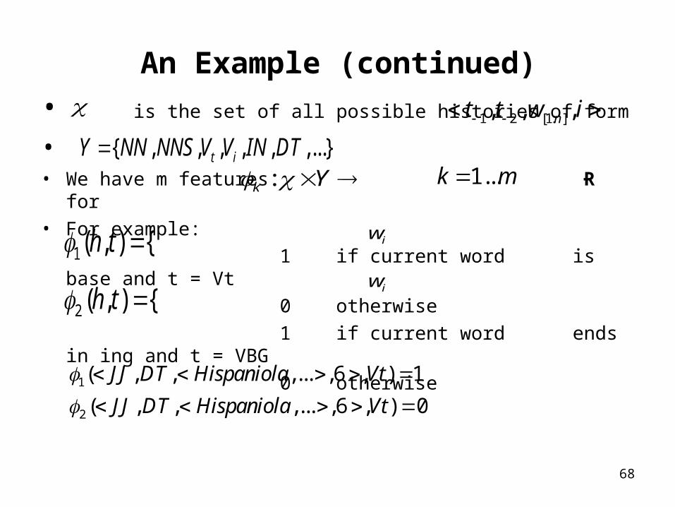
An Example (continued)
• is the set of all possible histories of form
• • We have m features Ɍ for• For example:
1 if current word is base and t = Vt
0 otherwise
1 if current word ends in ing and t = VBG
0 otherwise
1 2 [1: ], , ,nt t w i
{ , , , , , ,...}t iY NN NNS V V IN DT
:k Y 1...k m
1( , ) {h t iw
2 ( , ) {h t iw
1
2
( , , ,... ,6 , ) 1
( , , ,... ,6 , ) 0
JJ DT Hispaniola Vt
JJ DT Hispaniola Vt
69
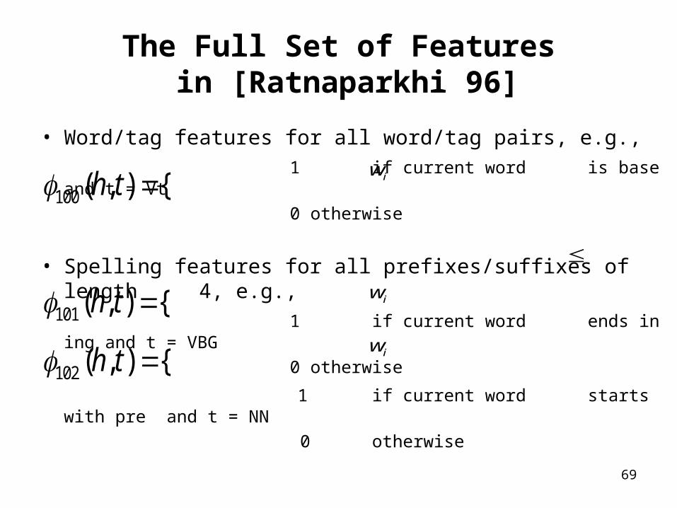
The Full Set of Features in [Ratnaparkhi 96]
• Word/tag features for all word/tag pairs, e.g.,
1 if current word is base and t = Vt
0 otherwise
• Spelling features for all prefixes/suffixes of length 4, e.g.,
1 if current word ends in ing and t = VBG
0 otherwise
1 if current word starts with pre and t = NN
0 otherwise
100 ( , ) {h t
101( , ) {h t
102 ( , ) {h t
iw
iw
iw
70
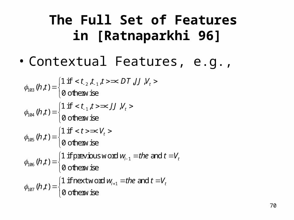
The Full Set of Features in [Ratnaparkhi 96]
• Contextual Features, e.g.,
2 1103
1104
105
1106
107
1 if , , , ,( , )
0 otherwise
1 if , ,( , )
0 otherwise
1 if ( , )
0 otherwise
1 if previous word and ( , )
0 otherwise
( ,
t
t
t
i t
t t t DT JJ Vh t
t t JJ Vh t
t Vh t
w the t Vh t
h t
11 if next word and )
0 otherwisei tw the t V
71
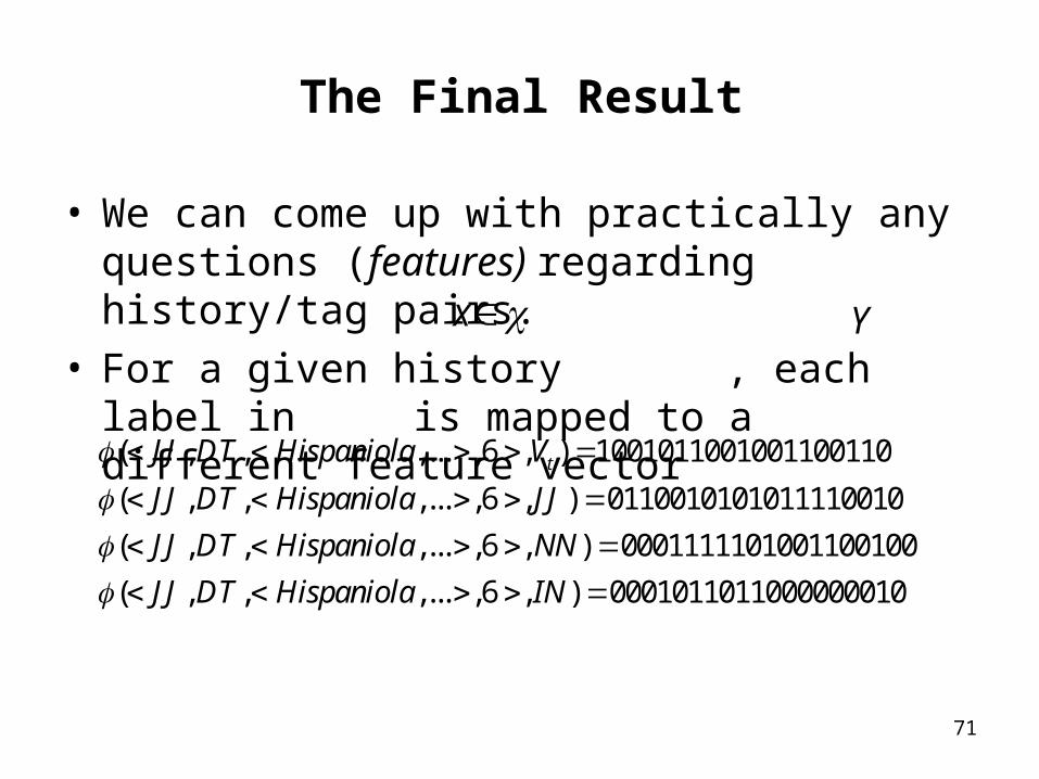
The Final Result
• We can come up with practically any questions (features) regarding history/tag pairs.
• For a given history , each label in is mapped to a different feature vector
( , , ,... ,6 , ) 1001011001001100110
( , , ,... ,6 , ) 0110010101011110010
( , , ,... ,6 , ) 0001111101001100100
( , , ,... ,6 , ) 00010110110
tJJ DT Hispaniola V
JJ DT Hispaniola JJ
JJ DT Hispaniola NN
JJ DT Hispaniola IN
00000010
x Y
72
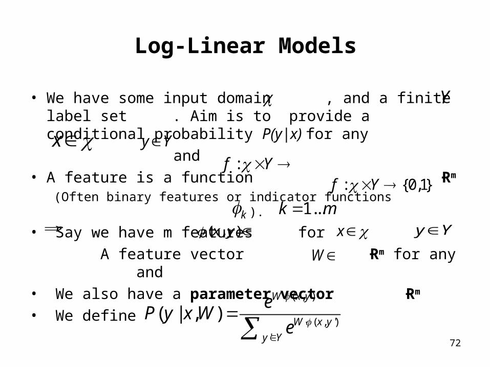
Log-Linear Models
• We have some input domain , and a finite label set . Aim is to provide a conditional probability P(y|x) for any
and • A feature is a function Ɍm
(Often binary features or indicator functions ).
• Say we have m features for
A feature vector Ɍm for any and• We also have a parameter vector Ɍm
• We define
Y
:f Y : {0,1}f Y
k 1...k m( , )x y x y Y
W
( , )
( , ')
'
( | , )W x y
W x y
y Y
eP y x W
e
x Yy
73
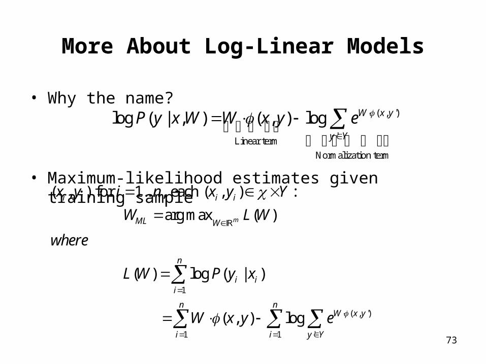
More About Log-Linear Models
• Why the name?
• Maximum-likelihood estimates given training sample
( , ')
'Linear term
Normalization term
log ( | , ) ( , ) log W x y
y Y
P y x W W x y e
1
( , ')
1 1 '
( , ) for 1... , each ( , ) :
arg max ( )
( ) log ( | )
( , ) log
m
i i i i
ML W
n
i ii
n nW x y
i i y Y
x y i n x y Y
W L W
where
L W P y x
W x y e
74
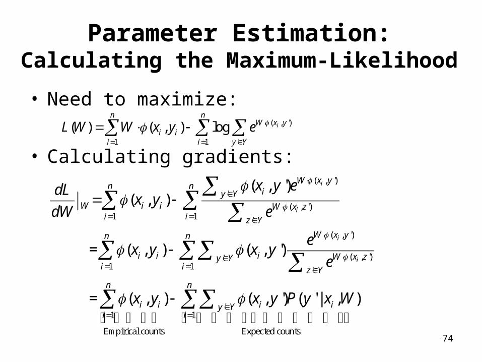
Parameter Estimation:Calculating the Maximum-Likelihood
• Need to maximize:
• Calculating gradients:
( , ')
1 1 '
( ) ( , ) log i
n nW x y
i ii i y Y
L W W x y e
( , ')
'
( , ')1 1 '
( , ')
( , ')'1 1 '
'1
Empirical counts
( , ')( , )
= ( , ) ( , ')
= ( , ) ( , ') ( ' |
i
i
i
i
W x yn n
iy YW i i W x z
i i z Y
W x yn n
i i i W x zy Yi i z Y
n
i i iy Yi
x y edLx y
dW e
ex y x y
e
x y x y P y x
1
Expected counts
, )n
ii
W
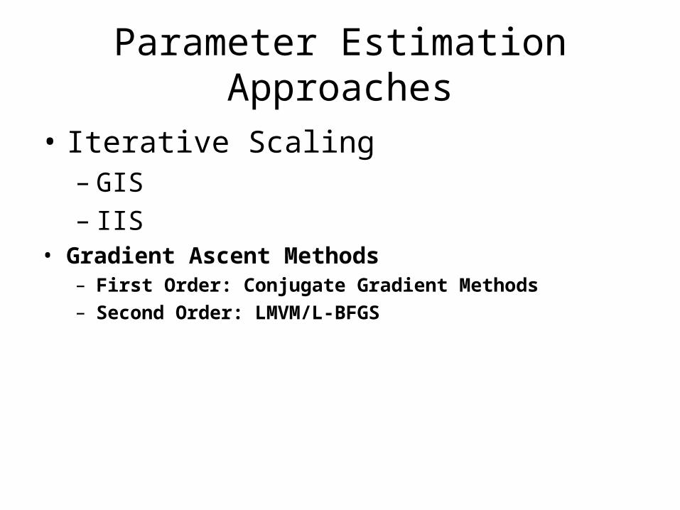
Parameter Estimation Approaches
• Iterative Scaling– GIS– IIS
• Gradient Ascent Methods– First Order: Conjugate Gradient Methods– Second Order: LMVM/L-BFGS
76
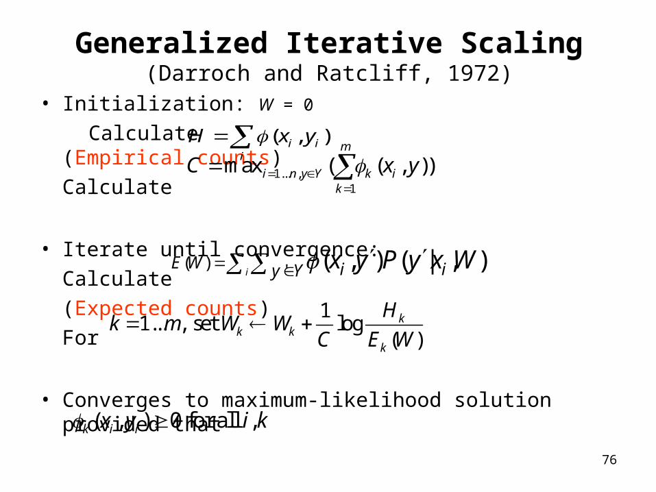
Generalized Iterative Scaling(Darroch and Ratcliff, 1972)
• Initialization: W = 0
Calculate (Empirical counts)
Calculate
• Iterate until convergence:
Calculate
(Expected counts)
For
• Converges to maximum-likelihood solution provided that
( , )i ii
x yH 1... ,
1
ma ( ))x ( ,m
i n y Y k ik
x yC
( ) ' ,( ) ( | , )i i iy YE W x y P y x W
11... , set
( )log k
k kk
WkW
Hm W
C E
0 for all ) ,( ,k i ix y i k
77
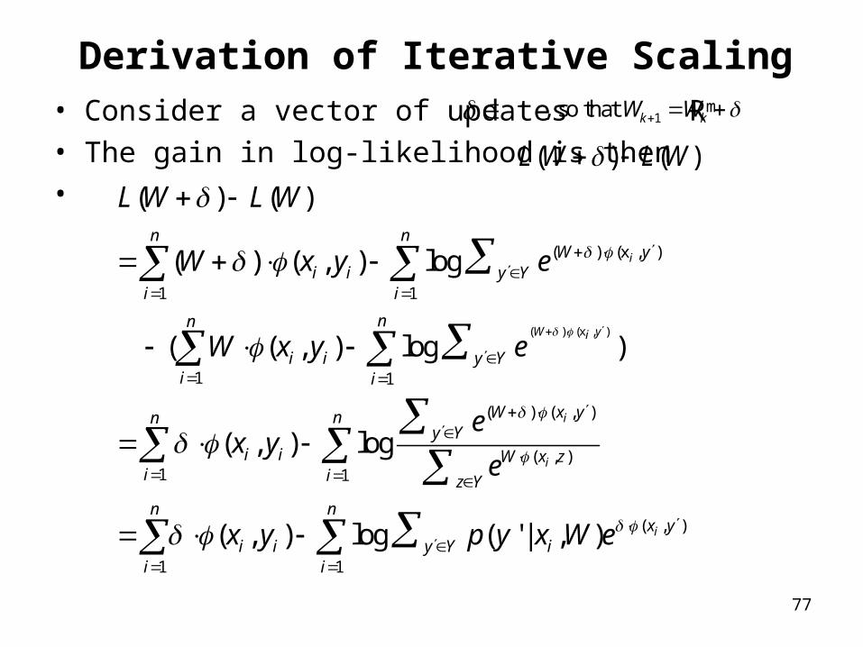
Derivation of Iterative Scaling• Consider a vector of updates Ɍm
• The gain in log-likelihood is then•
( ) ( )L W L W
( ) x , )(
(x
( ) ( )
(
( , )
) , )
1 1
1 1
,
1 1
1 1
( ) ( )
( log
( log )
) ( , )
( , )
( , lo)
( ,
g
l) og
i
W yi
i
i
n nW y
i i y Yi i
nn
i i y Yi i
ynny Y
i ii i Y
n n
i i y Yi i
W x
W x z
z
L W L W
W e
e
e
e
x y
W x y
x y
x y p
( , )( ' | , ) ix yiy x W e
1, so that k kW W
78
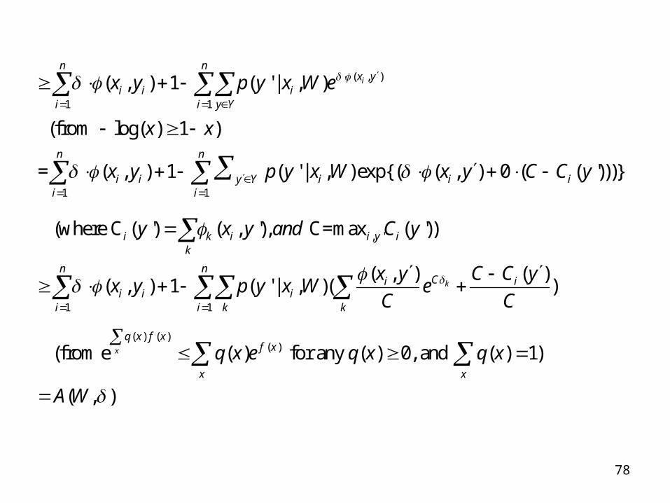
( , )
1 1
1 1
, '
1
( ' |
( ' | ( ')
( ') ( , '),
( , ) 1 , )
(from log( ) 1
C=max ( '))
)
= ( , ) 1 , ) exp{( ( , ) 0 ( ))}
(where C
( ,
i
n nx y
i i ii i y Y
n n
i i y Y i i ii i
i k i i y ik
n
ii
p y x
p y
x y W e
x x
x y
y x y a
x y W x y C
n
C
x
d C y
1
( ) ( )( )
, ) ( )) 1 , )( )
(from e
(( ' |
for any( ) ( ) 1) ( ) 0, and
( , )
k
x
nCi i
i ii k k
q x f xf x
x x
y C C yxp y x
C
q x
y W eC
q x e q x
A W
79
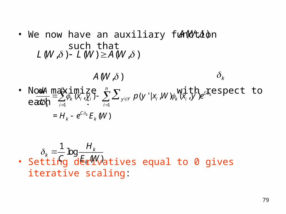
• We now have an auxiliary function such that
• Now maximize with respect to each :
• Setting derivatives equal to 0 gives iterative scaling:
( , )A W
( , )A W
) ( ) ( ,, )( L WL W A W
k
1 1
, ) , )( ( ' | (
= (
, )
)
k
k
n nC
k i i y Y i k ii ik
Ck k
dAx p y x x
d
H e E W
y W y e
1log
( )k
kk
H
WC E
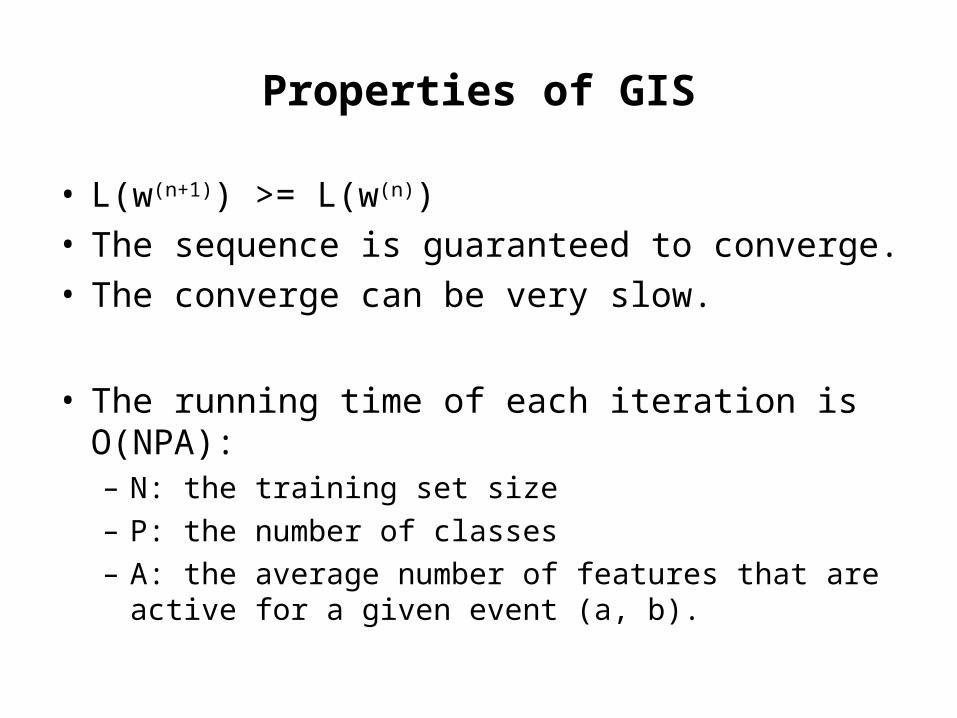
Properties of GIS
• L(w(n+1)) >= L(w(n))• The sequence is guaranteed to converge.• The converge can be very slow.
• The running time of each iteration is O(NPA):– N: the training set size– P: the number of classes– A: the average number of features that are active for
a given event (a, b).
81
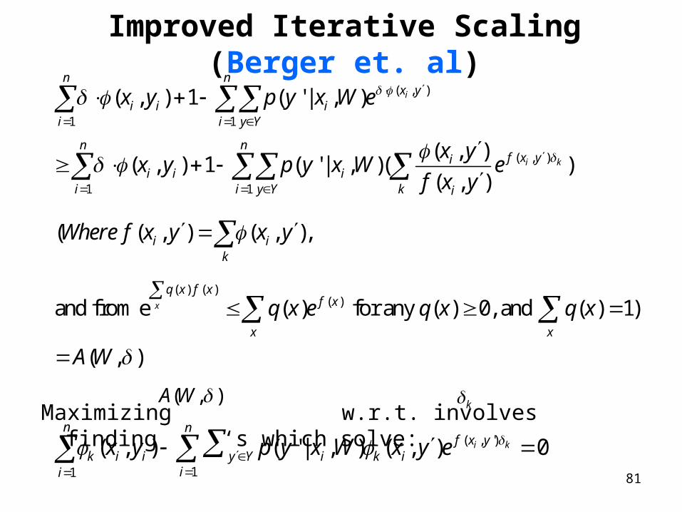
Improved Iterative Scaling (Berger et. al)
Maximizing w.r.t. involves finding ‘s which solve:
( , )
1 1
( , )
1 1
( ) ( )( )
( , ) 1 , )
, )( , ) 1 , )( )
( , )
( ( , ) , ),
and from e
( ' |
(( ' |
(
for any ( ) 0, and ( ) (
i
i k
x
n nx y
i i ii i y Y
n nf x yi
i i ii i y Y k i
i ik
q x f xf x
x
p y x
xp y x
x
q
x y W e
yx y W e
f x y
Where f x y
q qx
y
x e
) 1)
( , )x
x
A W
( , )A W k
( , ')
11
, ) ( ' | , ) ( , )( 0i k
n nf x y
k i i y Y i k iii
y p y x W xx y e
82
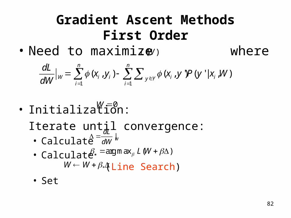
Gradient Ascent MethodsFirst Order
• Need to maximize where
• Initialization:
Iterate until convergence:• Calculate • Calculate (Line Search)• Set
'1 1
( , ) ( , ') ( ' | , )n n
W i i i iy Yi i
dLx y x y P y x W
dW
( )L W
0W
|WdL
dW
arg max ( )L W
*W W
83
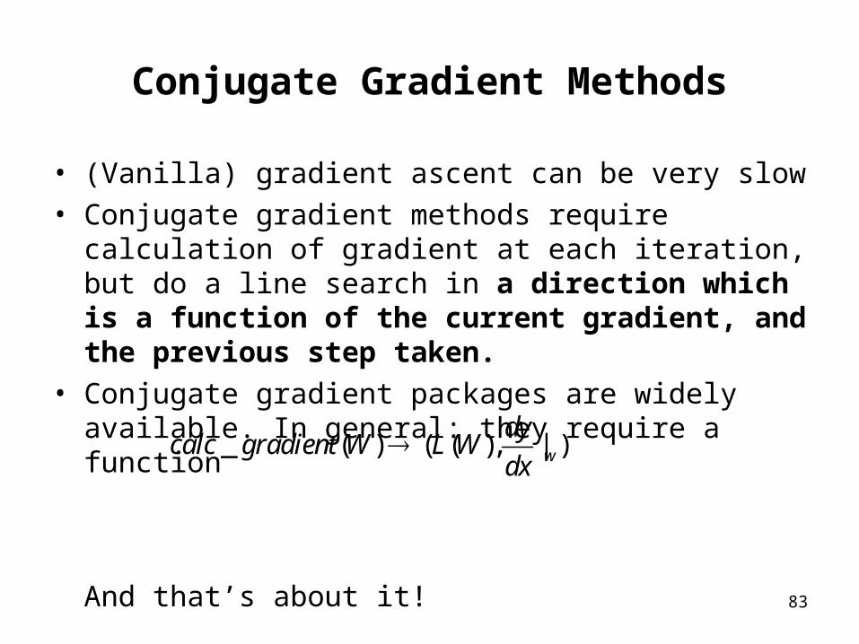
Conjugate Gradient Methods
• (Vanilla) gradient ascent can be very slow• Conjugate gradient methods require calculation of
gradient at each iteration, but do a line search in a direction which is a function of the current gradient, and the previous step taken.
• Conjugate gradient packages are widely available. In general: they require a function
And that’s about it!
_ ( ) ( ( ), )|wdy
calc gradient W L Wdx
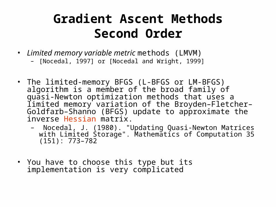
Gradient Ascent MethodsSecond Order
• Limited memory variable metric methods (LMVM)– [Nocedal, 1997] or [Nocedal and Wright, 1999]
• The limited-memory BFGS (L-BFGS or LM-BFGS) algorithm is a member of the broad family of quasi-Newton optimization methods that uses a limited memory variation of the Broyden–Fletcher–Goldfarb–Shanno (BFGS) update to approximate the inverse Hessian matrix.– Nocedal, J. (1980). "Updating Quasi-Newton Matrices with Limited
Storage". Mathematics of Computation 35 (151): 773–782
• You have to choose this type but its implementation is very complicated
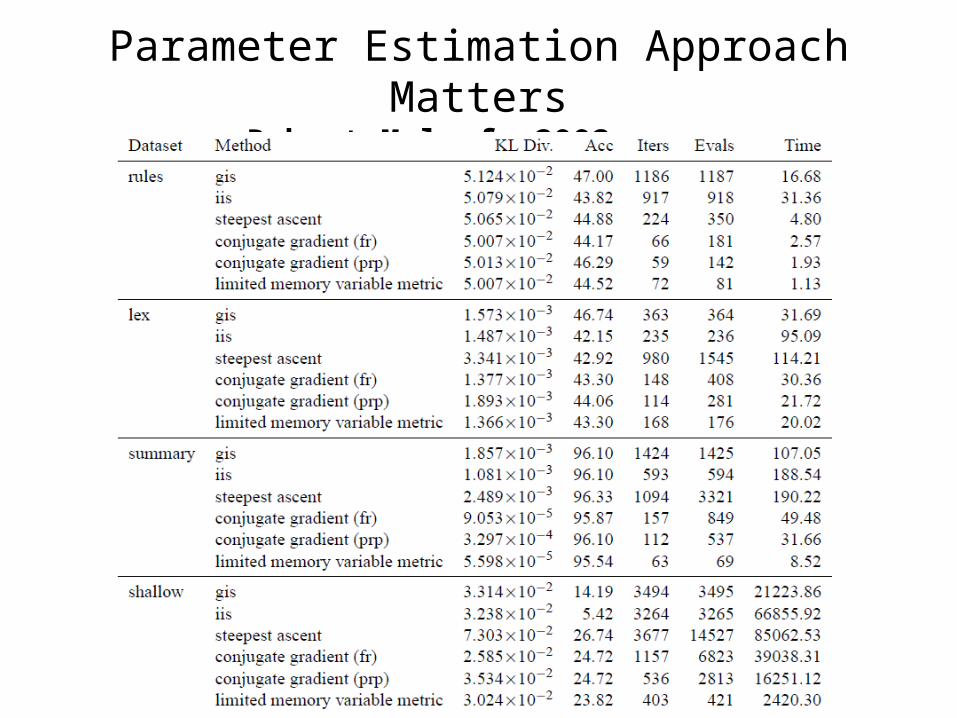
Parameter Estimation Approach Matters[Robert Malouf, 2002]@COLING
86
Overview
• Log-linear models
• The maximum-entropy property
• Smoothing, feature selection etc. in log-linear models
87
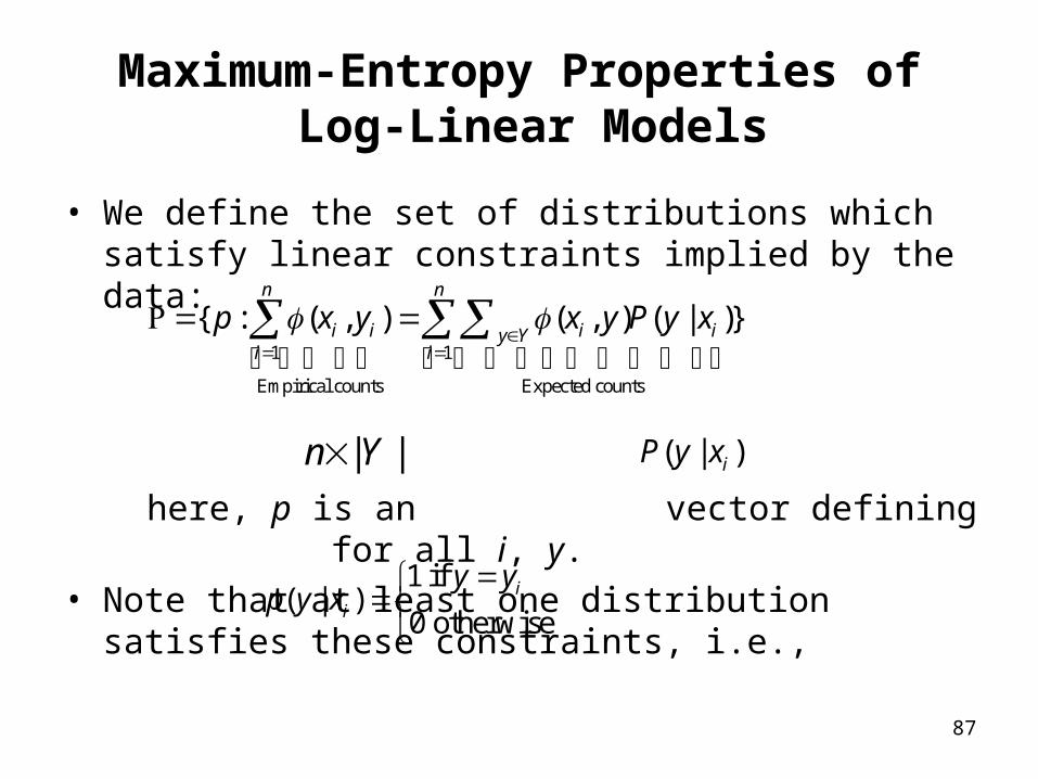
Maximum-Entropy Properties of Log-Linear Models
• We define the set of distributions which satisfy linear constraints implied by the data:
here, p is an vector defining for all i, y.• Note that at least one distribution satisfies these
constraints, i.e.,
1 1
Empirical counts Expected counts
{ : ( , ) ( , ) ( | )}n n
i i i iy Yi i
p x y x y P y x
| |n Y )( | iP y x
1 if ( |
0 otherwise) i
i
y yp y x
88
Maximum-Entropy Properties of Log-Linear Models
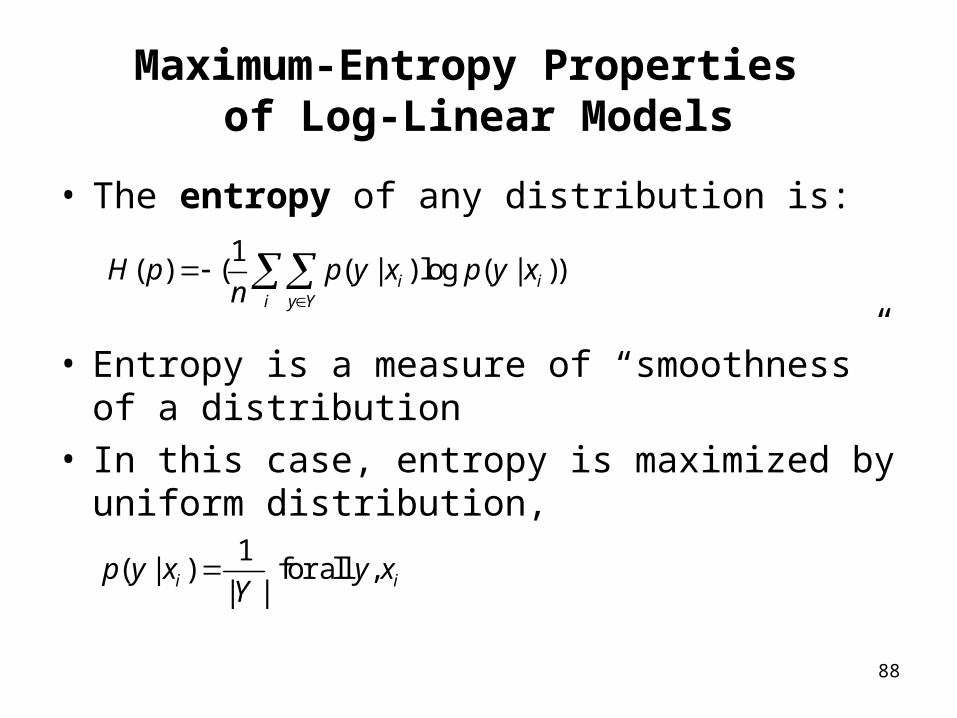
• The entropy of any distribution is:
• Entropy is a measure of “smoothness” of a distribution
• In this case, entropy is maximized by uniform distribution,
1( | ) log (( |( )) )i i
i y Y
p y x p y xn
H p
1) for all ,
| |( | i ip y x y x
Y
89
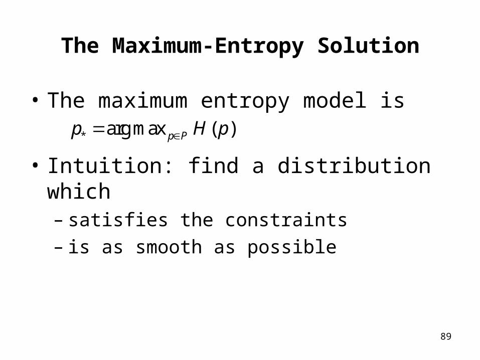
The Maximum-Entropy Solution
• The maximum entropy model is
• Intuition: find a distribution which– satisfies the constraints– is as smooth as possible
* arg max ( )p Pp H p
90
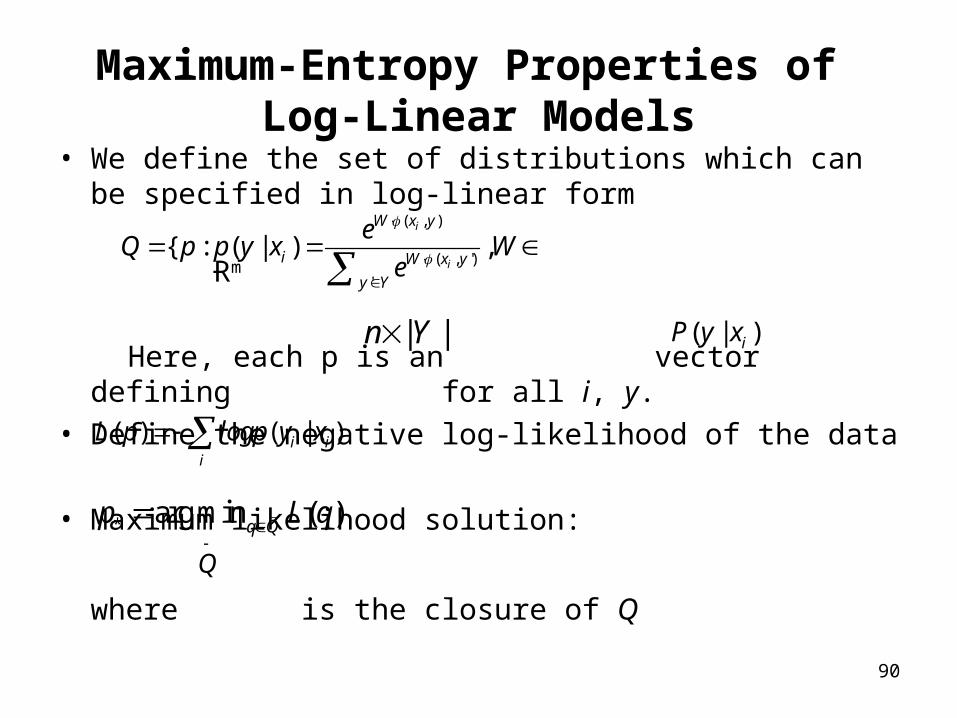
Maximum-Entropy Properties of Log-Linear Models
• We define the set of distributions which can be specified in log-linear form
Ɍm
Here, each p is an vector defining for all i, y.
• Define the negative log-likelihood of the data
• Maximum likelihood solution:
where is the closure of Q
( , )
( , ')
'
){ : ( | ,i
i
W x y
W x y
y
i
Y
eQ p p y x W
e
| |n Y )( | iP y x
|( () )i ii
logp yL xp
* arg min ( )q Qp L q
Q
91
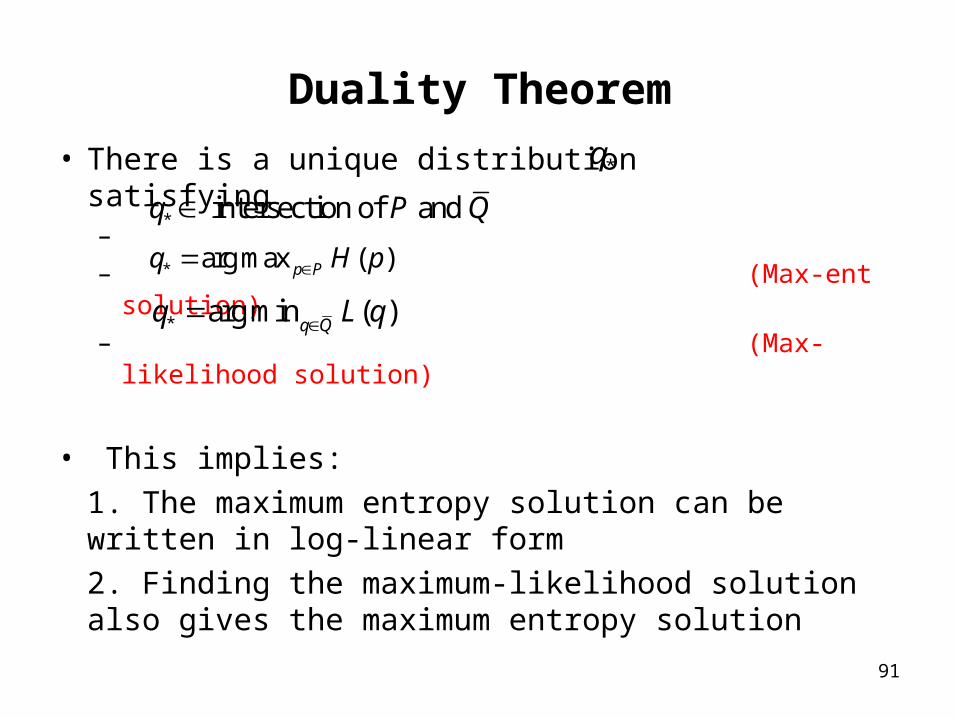
Duality Theorem
• There is a unique distribution satisfying– – (Max-ent solution) – (Max-likelihood solution)
• This implies:
1. The maximum entropy solution can be written in log-linear form
2. Finding the maximum-likelihood solution also gives the maximum entropy solution
*q
* intersection of and P Qq
* arg min ( )q Qq L q* arg max ( )p Pq H p
92
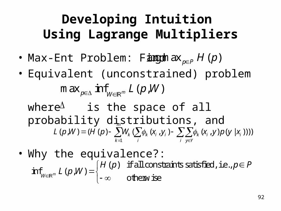
Developing Intuition Using Lagrange Multipliers
• Max-Ent Problem: Find• Equivalent (unconstrained) problem
where is the space of all probability distributions, and
• Why the equivalence?:
arg max ( )p P H p
max inf ( , )mp WL p W
1
( , ) , ) (( , ) ( ( ) ( ( | )) ))m
k k i i k i ik i i y Y
x y y p yL p W H p W x x
( ) if all constraints satisfied, i.e., inf ( , )
otherwise mW
H p p PL p W
93
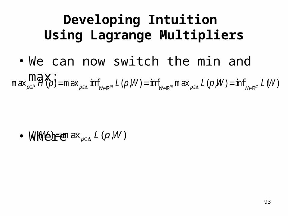
Developing Intuition Using Lagrange Multipliers
• We can now switch the min and max:
• Where
max ( ) max inf ( , ) inf max ( , ) inf ( )m m mp P p pW W WH p L p W L p W L W
( ) max ( , )pL W L p W
94
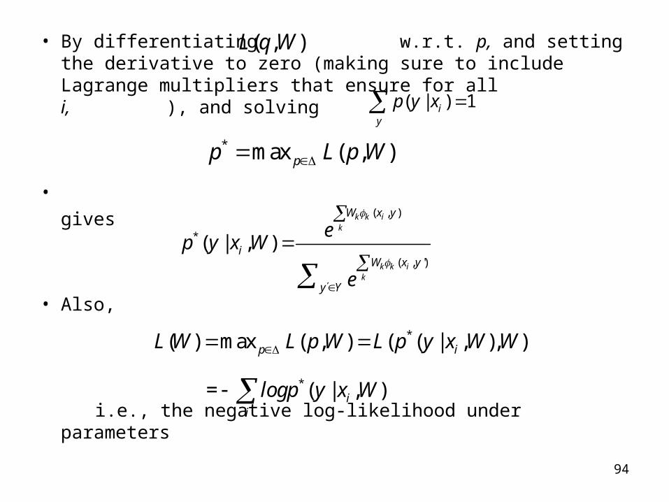
• By differentiating w.r.t. p, and setting the derivative to zero (making sure to include Lagrange multipliers that ensure for all i, ), and solving
•
gives
• Also,
i.e., the negative log-likelihood under parameters
( , )L q W
( | ) 1iy
p y x * max ( , )pp L p W
,( )
*
( , ')
, )( |
k k ik
k k ik
y
iy
y Y
W x
W x
Wp y x
e
e
*
*
, ), )
( ) ma
x ( ,
= ( |
) ( ( |
, )
p i
ii
L W L p W L p W W
logp y W
y x
x
95
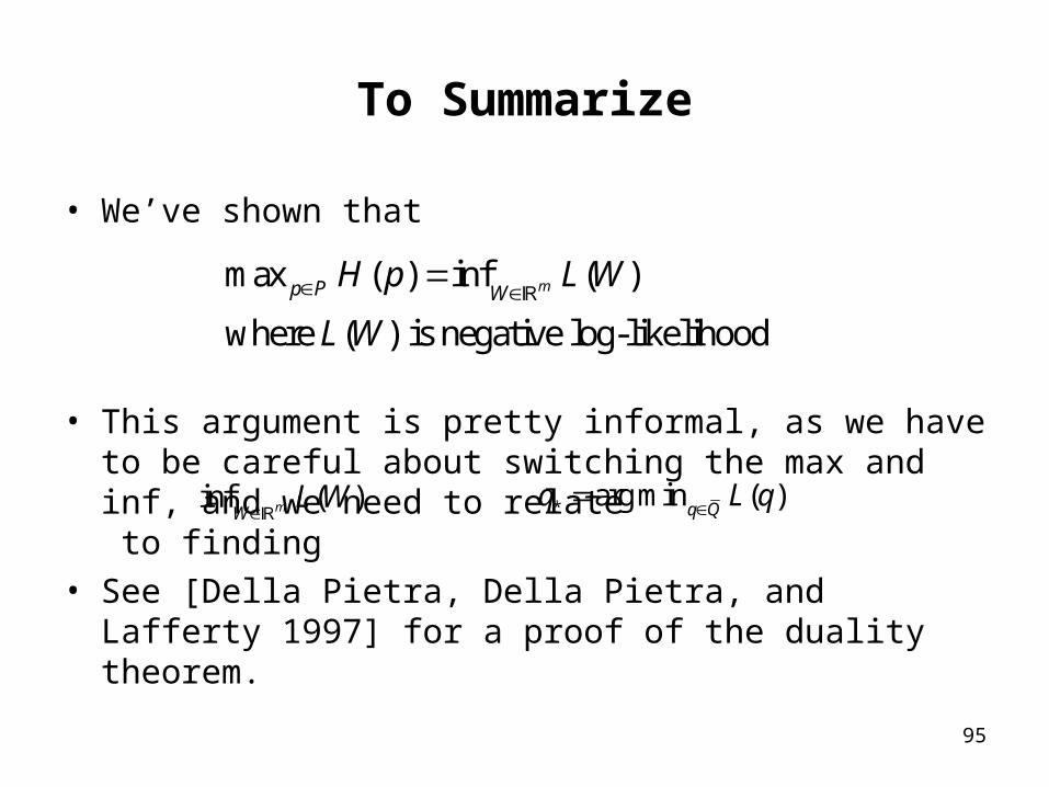
To Summarize
• We’ve shown that
• This argument is pretty informal, as we have to be careful about switching the max and inf, and we need to relate to finding
• See [Della Pietra, Della Pietra, and Lafferty 1997] for a proof of the duality theorem.
max ( ) inf ( )
where ( ) is negative log-likelihood
mp P WH p L W
L W
inf ( )mWL W
* arg min ( )q Qq L q
96
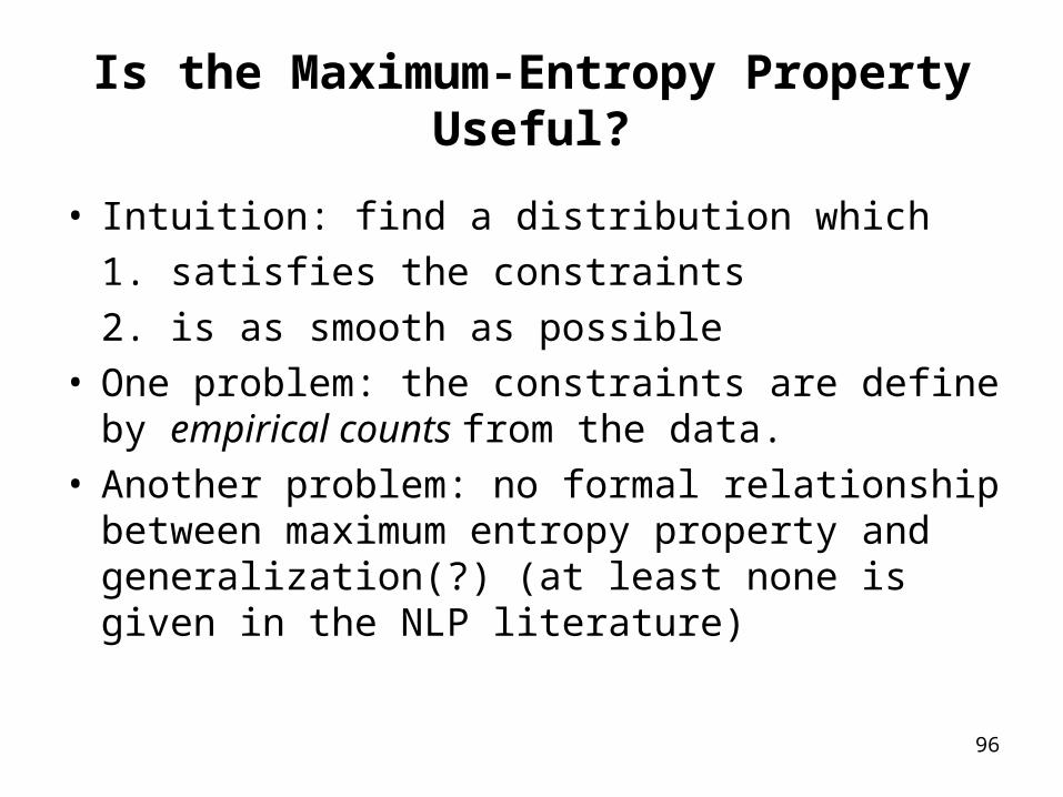
Is the Maximum-Entropy Property Useful?
• Intuition: find a distribution which
1. satisfies the constraints
2. is as smooth as possible• One problem: the constraints are define by
empirical counts from the data.• Another problem: no formal relationship between
maximum entropy property and generalization(?) (at least none is given in the NLP literature)
97
Overview
• Log-linear models
• The maximum-entropy property
• Smoothing, feature selection etc. in log-linear models
98
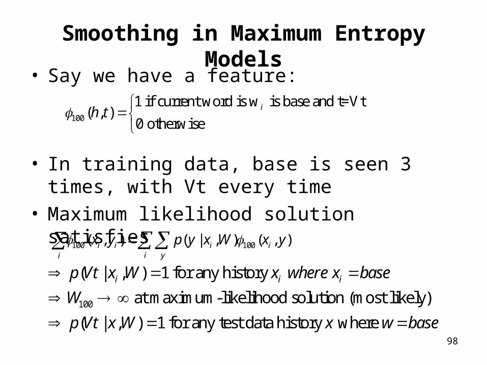
Smoothing in Maximum Entropy Models• Say we have a feature:
• In training data, base is seen 3 times, with Vt every time
• Maximum likelihood solution satisfies
100
1 if current word i is base and s w(
t=Vt, )
0 otherwiseih t
100 100( , ) ( | , ) ( , )i i i ii yi
p y xx y x yW
100
at maximum-likelihood solution (most likely
( | , ) 1 for any history
)
( | , ) 1 for any test data hist
ory where
i i ix where x base
W
p
p Vt x W
Vt x W x w base
99
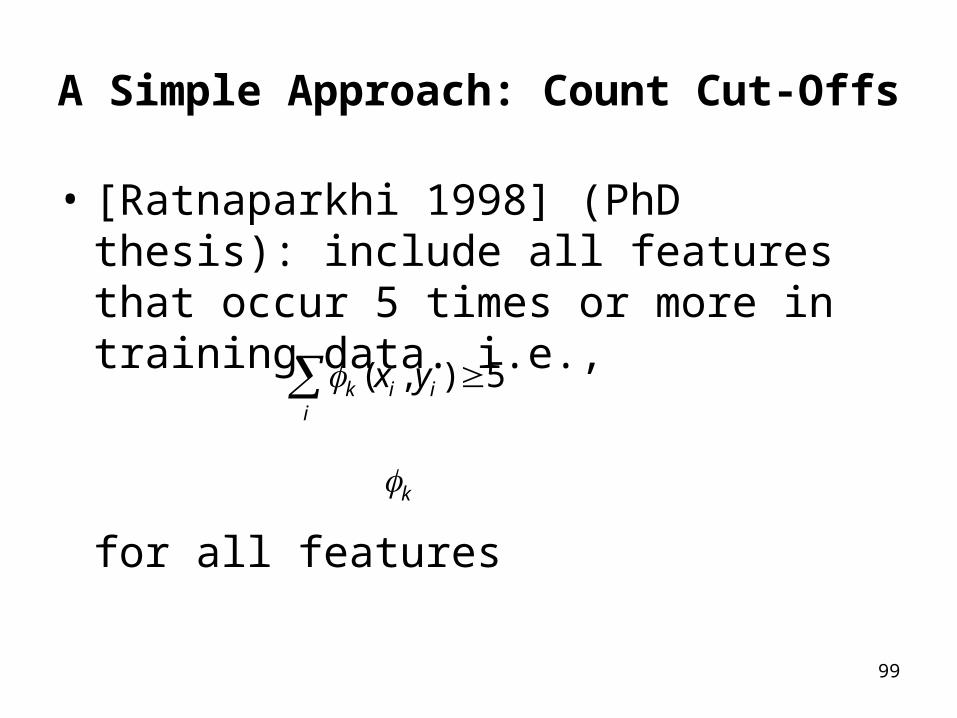
A Simple Approach: Count Cut-Offs
• [Ratnaparkhi 1998] (PhD thesis): include all features that occur 5 times or more in training data. i.e.,
for all features k
, )( 5k i ii
yx
100
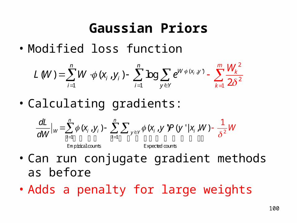
Gaussian Priors
• Modified loss function
• Calculating gradients:
• Can run conjugate gradient methods as before
• Adds a penalty for large weights
( , ')
1 '2
1
2
1
( ) ( , ) log2
i
mk
k
n nW x
ii y Y
iy
i
WL W W x y e
'1 1
Empirical counts Expected count
2
s
( , ) ( , ') ( ' | ,1
)n n
W i i i iy Yi i
dLx y x y P Wy x W
dW
101
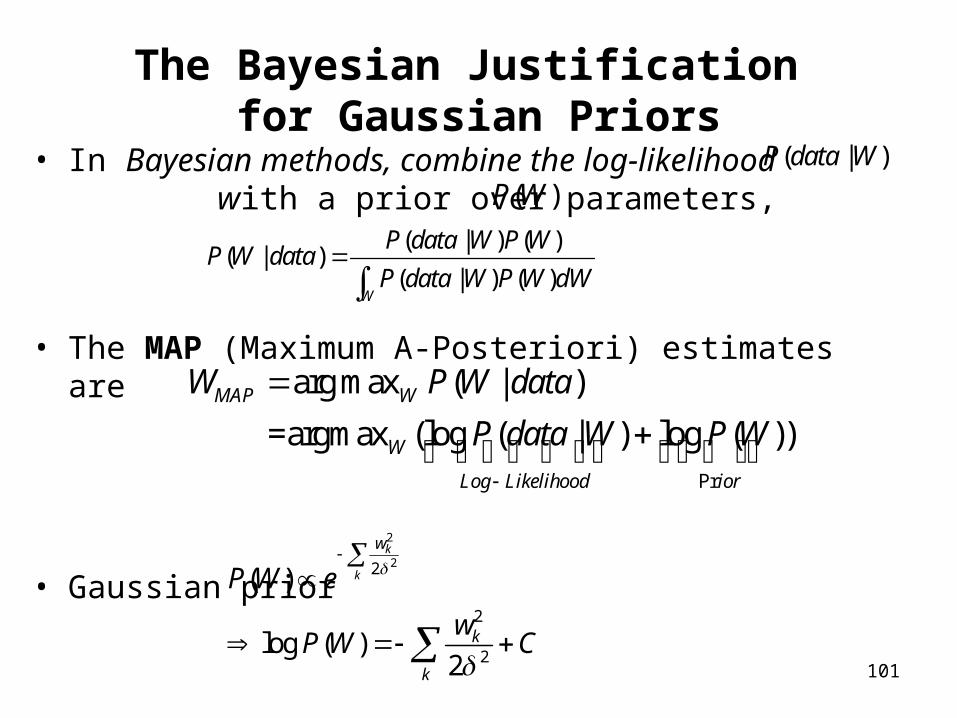
The Bayesian Justification for Gaussian Priors
• In Bayesian methods, combine the log-likelihood with a prior over parameters,
• The MAP (Maximum A-Posteriori) estimates are
• Gaussian prior
( | )P data W
( )P W
( | ) ( )( | )
( | ) ( )W
P data W P WP W data
P data W P W dW
Pr
arg max ( | )
=argmax (log ( | ) log ( ))Log Likelihood ior
MAP W
W
W P W data
P data W P W
2
22
2
2
( )
log ( )2
k
k
w
k
k
P W e
P Ww
C
102
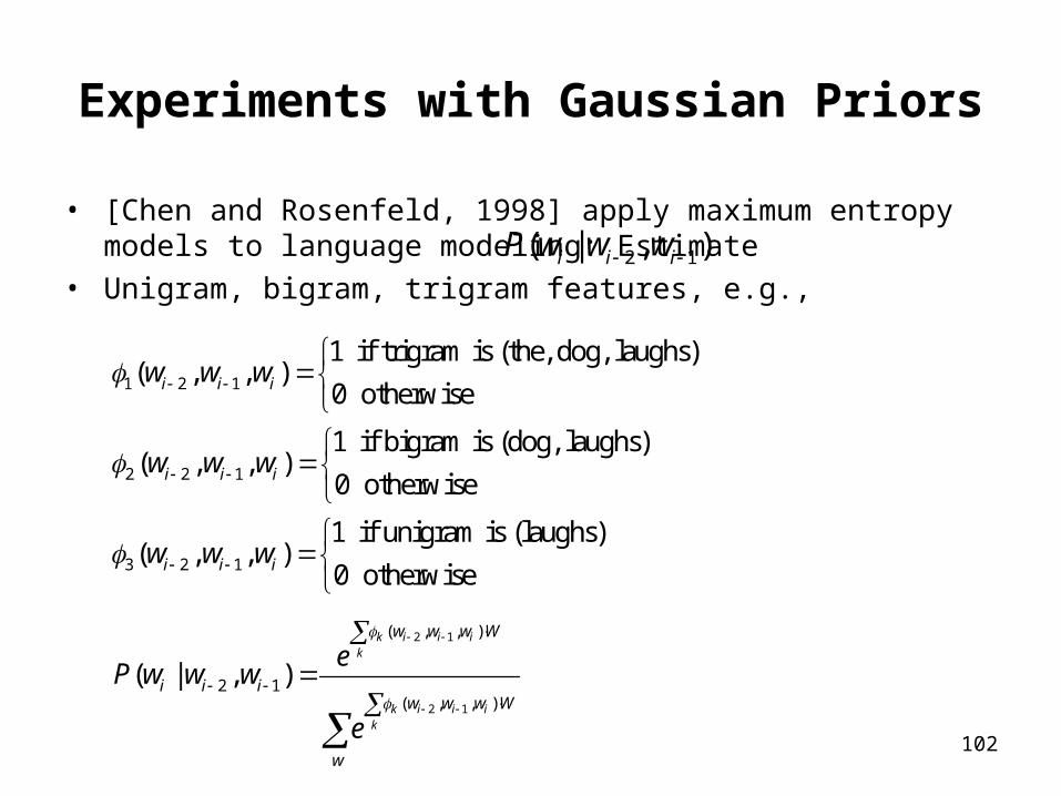
Experiments with Gaussian Priors
• [Chen and Rosenfeld, 1998] apply maximum entropy models to language modeling: Estimate
• Unigram, bigram, trigram features, e.g.,2 1( | , )i i iP w ww
1 2 1
2 1
2 1
2 1
2
3
1 if trigram is (the, dog, laughs)( , , )
0 otherwise
1 if bigram is (dog, laughs)( , , )
0 otherwise
1 if unigram is (laughs)( , , )
0 otherwise
( | , )
i i i
i i i
i i i
i i i
w w w
w w w
w w w
P w w w
2 1
2 1
( , , )
( , , )
k i i ik
k i i ik
w
w w w W
w w w W
e
e
103
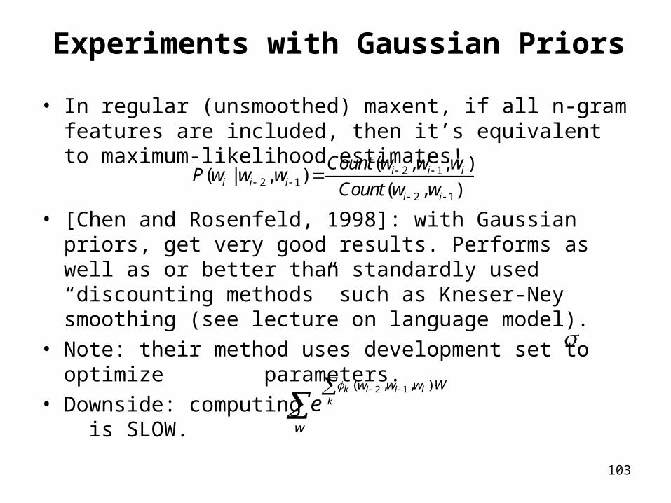
Experiments with Gaussian Priors
• In regular (unsmoothed) maxent, if all n-gram features are included, then it’s equivalent to maximum-likelihood estimates!
• [Chen and Rosenfeld, 1998]: with Gaussian priors, get very good results. Performs as well as or better than standardly used “discounting methods” such as Kneser-Ney smoothing (see lecture on language model).
• Note: their method uses development set to optimize parameters.
• Downside: computing is SLOW.
2 1( , , )k i i ik
w w w
w
W
e
2 12 1
2 1
( , , )( | , )
( , )i i i
i i ii i
Count w w wP w w w
Count w w
104
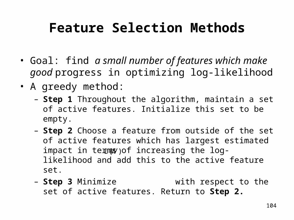
Feature Selection Methods
• Goal: find a small number of features which make good progress in optimizing log-likelihood
• A greedy method:– Step 1 Throughout the algorithm, maintain a set of active
features. Initialize this set to be empty.– Step 2 Choose a feature from outside of the set of active
features which has largest estimated impact in terms of increasing the log-likelihood and add this to the active feature set.
– Step 3 Minimize with respect to the set of active features. Return to Step 2.
( )L W
105
Experimental Results from [Ratnaparkhi 1998] (PhD thesis)
• The task: PP attachment ambiguity• ME Default: Count cut-off of 5• ME Tuned: Count cut-offs vary for 4-tuples, 3-tuples, 2-
tuples, unigram features• ME IFS: feature selection method
106
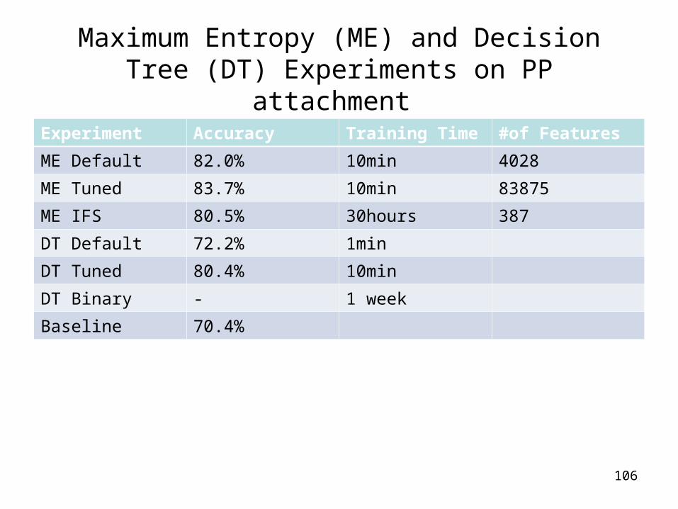
Maximum Entropy (ME) and Decision Tree (DT) Experiments on PP attachment
Experiment Accuracy Training Time #of Features
ME Default 82.0% 10min 4028
ME Tuned 83.7% 10min 83875
ME IFS 80.5% 30hours 387
DT Default 72.2% 1min
DT Tuned 80.4% 10min
DT Binary - 1 week
Baseline 70.4%
107
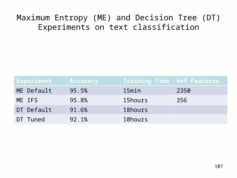
Maximum Entropy (ME) and Decision Tree (DT) Experiments on text classification
Experiment Accuracy Training Time #of Features
ME Default 95.5% 15min 2350
ME IFS 95.8% 15hours 356
DT Default 91.6% 18hours
DT Tuned 92.1% 10hours
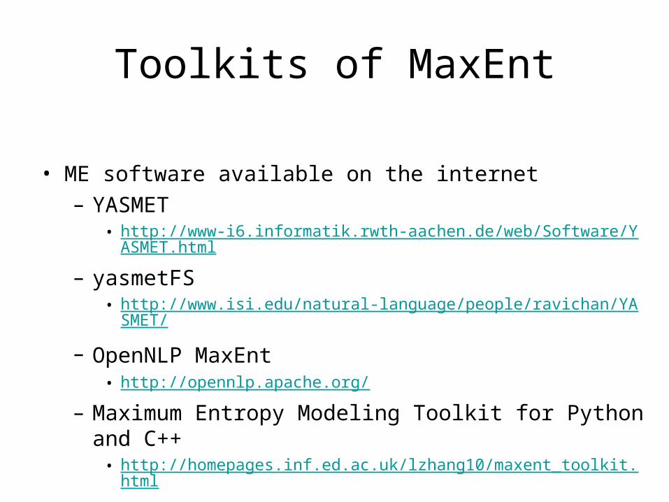
Toolkits of MaxEnt
• ME software available on the internet– YASMET
• http://www-i6.informatik.rwth-aachen.de/web/Software/YASMET.html
– yasmetFS• http://www.isi.edu/natural-language/people/ravichan/YASMET/
– OpenNLP MaxEnt • http://opennlp.apache.org/
– Maximum Entropy Modeling Toolkit for Python and C++• http://homepages.inf.ed.ac.uk/lzhang10/maxent_toolkit.html
109
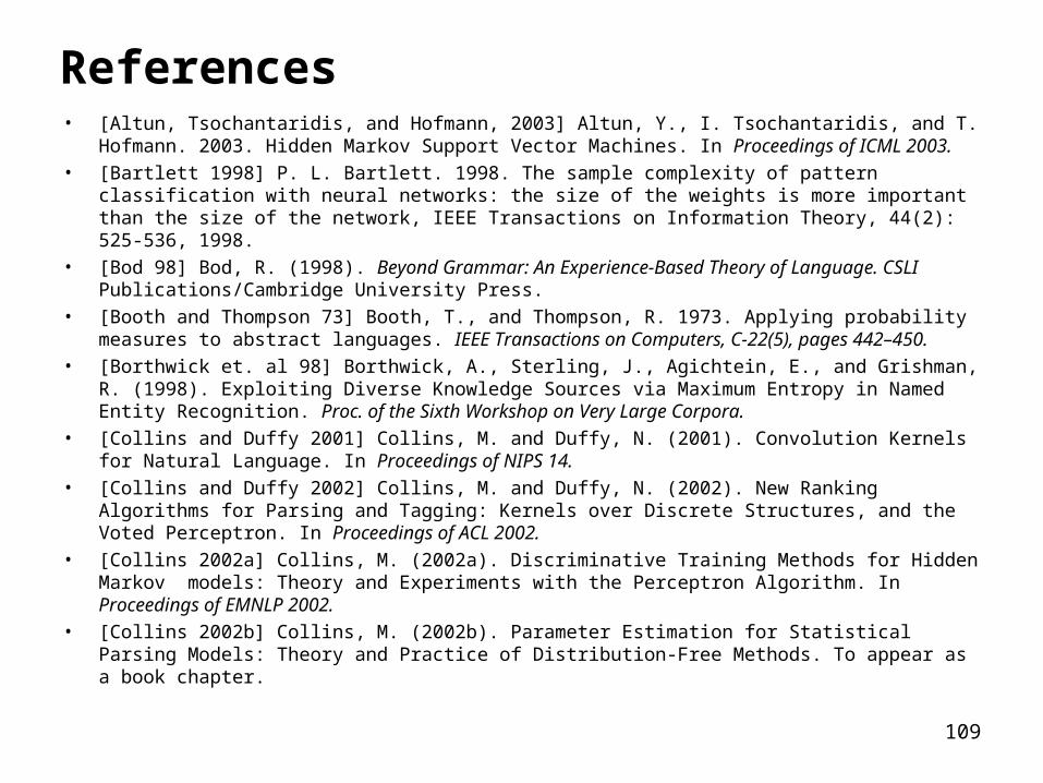
References• [Altun, Tsochantaridis, and Hofmann, 2003] Altun, Y., I. Tsochantaridis, and T. Hofmann. 2003.
Hidden Markov Support Vector Machines. In Proceedings of ICML 2003.
• [Bartlett 1998] P. L. Bartlett. 1998. The sample complexity of pattern classification with neural networks: the size of the weights is more important than the size of the network, IEEE Transactions on Information Theory, 44(2): 525-536, 1998.
• [Bod 98] Bod, R. (1998). Beyond Grammar: An Experience-Based Theory of Language. CSLI Publications/Cambridge University Press.
• [Booth and Thompson 73] Booth, T., and Thompson, R. 1973. Applying probability measures to abstract languages. IEEE Transactions on Computers, C-22(5), pages 442–450.
• [Borthwick et. al 98] Borthwick, A., Sterling, J., Agichtein, E., and Grishman, R. (1998). Exploiting Diverse Knowledge Sources via Maximum Entropy in Named Entity Recognition. Proc. of the Sixth Workshop on Very Large Corpora.
• [Collins and Duffy 2001] Collins, M. and Duffy, N. (2001). Convolution Kernels for Natural Language. In Proceedings of NIPS 14.
• [Collins and Duffy 2002] Collins, M. and Duffy, N. (2002). New Ranking Algorithms for Parsing and Tagging: Kernels over Discrete Structures, and the Voted Perceptron. In Proceedings of ACL 2002.
• [Collins 2002a] Collins, M. (2002a). Discriminative Training Methods for Hidden Markov models: Theory and Experiments with the Perceptron Algorithm. In Proceedings of EMNLP 2002.
• [Collins 2002b] Collins, M. (2002b). Parameter Estimation for Statistical Parsing Models: Theory and Practice of Distribution-Free Methods. To appear as a book chapter.
110
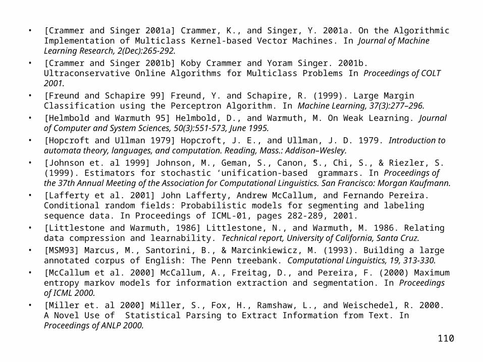
• [Crammer and Singer 2001a] Crammer, K., and Singer, Y. 2001a. On the Algorithmic Implementation of Multiclass Kernel-based Vector Machines. In Journal of Machine Learning Research, 2(Dec):265-292.
• [Crammer and Singer 2001b] Koby Crammer and Yoram Singer. 2001b. Ultraconservative Online Algorithms for Multiclass Problems In Proceedings of COLT 2001.
• [Freund and Schapire 99] Freund, Y. and Schapire, R. (1999). Large Margin Classification using the Perceptron Algorithm. In Machine Learning, 37(3):277–296.
• [Helmbold and Warmuth 95] Helmbold, D., and Warmuth, M. On Weak Learning. Journal of Computer and System Sciences, 50(3):551-573, June 1995.
• [Hopcroft and Ullman 1979] Hopcroft, J. E., and Ullman, J. D. 1979. Introduction to automata theory, languages, and computation. Reading, Mass.: Addison–Wesley.
• [Johnson et. al 1999] Johnson, M., Geman, S., Canon, S., Chi, S., & Riezler, S. (1999). Estimators for stochastic ‘unification-based” grammars. In Proceedings of the 37th Annual Meeting of the Association for Computational Linguistics. San Francisco: Morgan Kaufmann.
• [Lafferty et al. 2001] John Lafferty, Andrew McCallum, and Fernando Pereira. Conditional random fields: Probabilistic models for segmenting and labeling sequence data. In Proceedings of ICML-01, pages 282-289, 2001.
• [Littlestone and Warmuth, 1986] Littlestone, N., and Warmuth, M. 1986. Relating data compression and learnability. Technical report, University of California, Santa Cruz.
• [MSM93] Marcus, M., Santorini, B., & Marcinkiewicz, M. (1993). Building a large annotated corpus of English: The Penn treebank. Computational Linguistics, 19, 313-330.
• [McCallum et al. 2000] McCallum, A., Freitag, D., and Pereira, F. (2000) Maximum entropy markov models for information extraction and segmentation. In Proceedings of ICML 2000.
• [Miller et. al 2000] Miller, S., Fox, H., Ramshaw, L., and Weischedel, R. 2000. A Novel Use of Statistical Parsing to Extract Information from Text. In Proceedings of ANLP 2000.
111
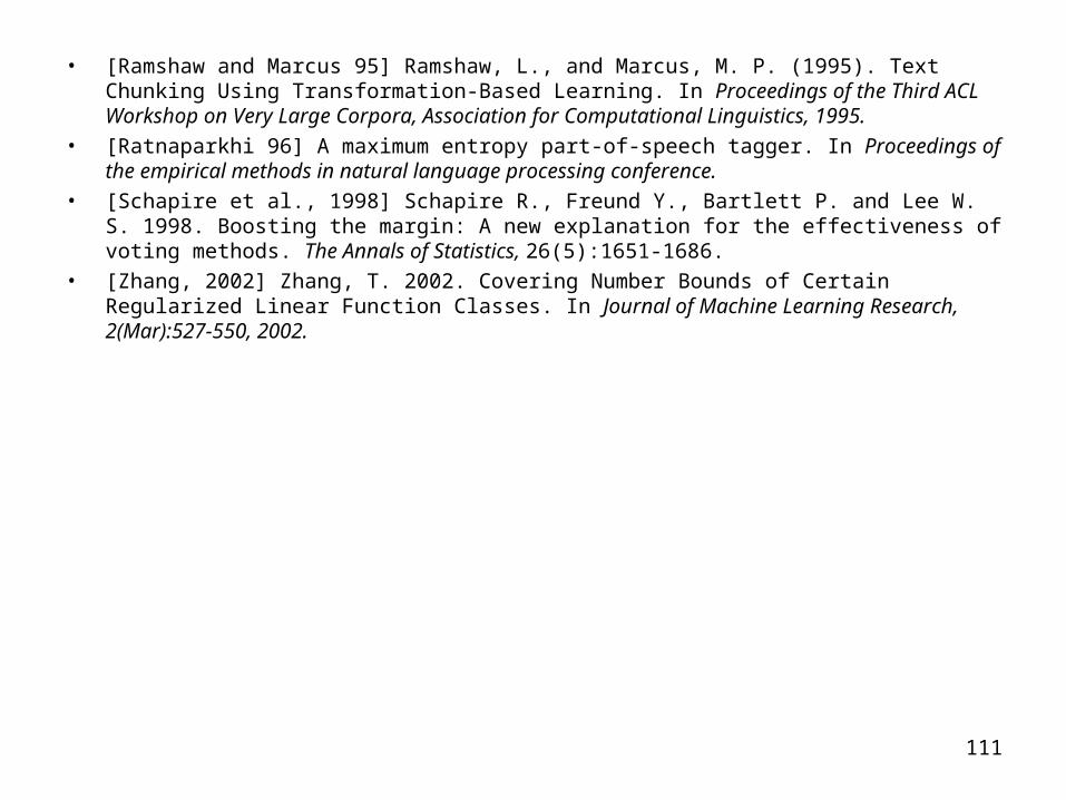
• [Ramshaw and Marcus 95] Ramshaw, L., and Marcus, M. P. (1995). Text Chunking Using Transformation-Based Learning. In Proceedings of the Third ACL Workshop on Very Large Corpora, Association for Computational Linguistics, 1995.
• [Ratnaparkhi 96] A maximum entropy part-of-speech tagger. In Proceedings of the empirical methods in natural language processing conference.
• [Schapire et al., 1998] Schapire R., Freund Y., Bartlett P. and Lee W. S. 1998. Boosting the margin: A new explanation for the effectiveness of voting methods. The Annals of Statistics, 26(5):1651-1686.
• [Zhang, 2002] Zhang, T. 2002. Covering Number Bounds of Certain Regularized Linear Function Classes. In Journal of Machine Learning Research, 2(Mar):527-550, 2002.