June 19, 2018

Naturalness, Extra-Empirical Theory Assessments,and the Implications of Skepticism1

James D. Wells

Leinweber Center for Theoretical PhysicsPhysics Department, University of Michigan

Ann Arbor, MI 48109-1040 USA

Abstract: Naturalness is an extra-empirical quality that aims to assess plausibility of a theory.Finetuning measures are one way to quantify the task. However, knowing statistical distri-butions on parameters appears necessary for rigor. Such meta-theories are not known yet.A critical discussion of these issues is presented, including their possible resolutions in fixedpoints. Skepticism of naturalness’s utility remains credible, as is skepticism to any extra-empirical theory assessment (SEETA) that claims to identify “more correct” theories that areequally empirically adequate. Specifically to naturalness, SEETA implies that one must ac-cept all concordant theory points as a priori equally plausible, with the practical implicationthat a theory can never have its plausibility status diminished by even a “massive reduction”of its viable parameter space as long as a single theory point still survives. A second implica-tion of SEETA suggests that only falsifiable theories allow their plausibility status to change,but only after discovery or after null experiments with total theory coverage. And a thirdimplication of SEETA is that theory preference then becomes not about what theory is morecorrect but what theory is practically more advantageous, such as fewer parameters, easier tocalculate, or has new experimental signatures to pursue.

1Based on lecture presented at the workshop “Naturalness, Hierarchy, and Finetuning”, Aachen, Germany,28 February 2018.

1

1 Extra-empirical attributes of theories

Empirical adequacy 2 is the pre-eminent requirement of a theory. However, a key problem inscience is the underdetermination of theory based on observed phenomena. Many theories, infact an infinite number of theories, are consistent with all known observations. This assertionmay be qualitatively true, but assuredly it is technically true when we realize that thereare a finite number of observations made to compare with theory, and all observations haveuncertainty (e.g., the mass of the Z boson is MZ = 91.1176± 0.0021 GeV [2]).

Faced with a large number of concordant theories (i.e., equally empirically adequate), onelooks to additional extra-empirical criteria to further refine assessments of their value. Theseextra-empirical attributes to theories include simplicity, testability, falsifiability, naturalness,calculability, and diversity. None of these attributes has been proven to be logically necessaryfor an authentic theory, although an authentic theory may possess them. However, there stillmay be important reasons to evoke these considerations in the pursuit of scientific progress.For example, a scientist may wish to make a discovery in his/her lifetime, in which casepromptly testable theories are more important to work on than theories judged to be morelikely but not promptly testable. Or, a scientist may wish to widen her vision of observableconsequences of concordant theories in order to cast a wider experimental net, which wouldlead her to pursue diverse theories over simple theories.

Another preference might be to identify the subset of concordant theory(ies) most likely tobe authentic among the much larger collection of concordant theories. Simplicity, falsifiability,calculability, etc., are all not reliable guides to answer this question. However, among theextra-empirical attributes naturalness [3, 4, 5, 6, 7, 8, 9] is the one that most directly speaksto this goal. If the naturalness of a theory has any value at all, it is because it appeals to ourquest to sort concordant theories into likely and unlikely candidates – natural and unnaturaltheories.

2 Finetuning functional

In practice, naturalness is often closely tied to notions of finetuning. A theory is unnatural ifits parameters require a high degree of finetuning to match observables or other parameterswhen matching across effective theories (EFTs), and a theory is natural otherwise. One firstconstructs a finetuning functional FT on a theory T to map the theory to a number FT [T ],which is its finetuning. For example, let us denote a set of parameters of the theory by xi,and a set of observables by Ok. A candidate finetuning functional could be [10, 11]

FT [T ] = max∑ik

∣∣∣∣ xiOk

∂Ok

∂xi

∣∣∣∣ . (1)

The higher the value of FT [T ] the more finetuned it is and the less likely it is to be natural,according to this algorithm. For example, one could decide that a theory is natural, or “FT-

2Italicized words appearing in this article are defined in more detail in [1].

2

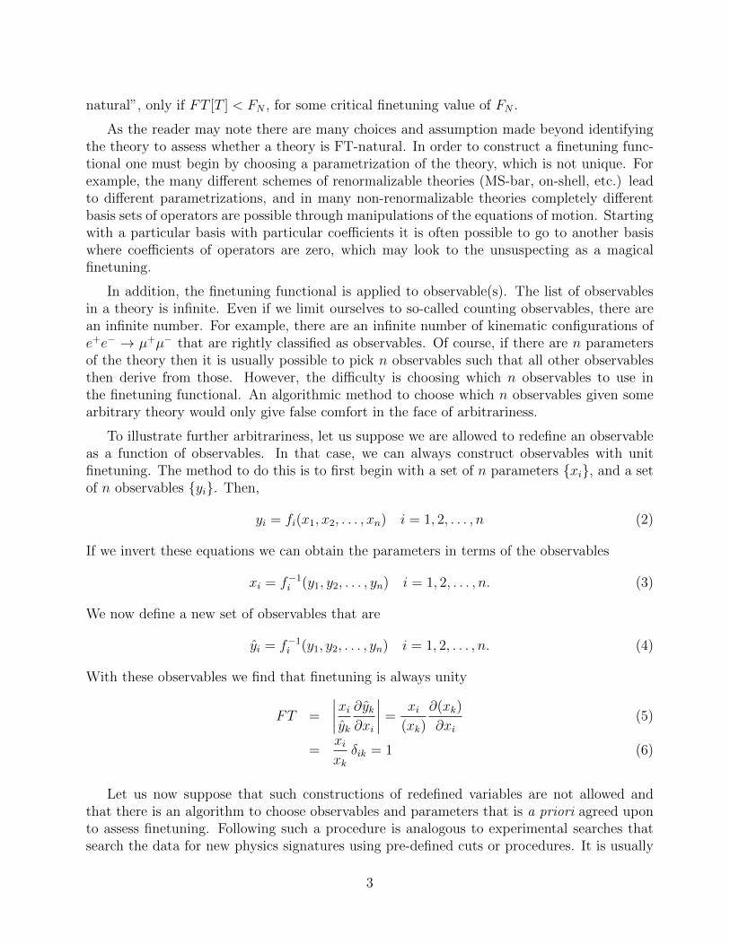
natural”, only if FT [T ] < FN , for some critical finetuning value of FN .

As the reader may note there are many choices and assumption made beyond identifyingthe theory to assess whether a theory is FT-natural. In order to construct a finetuning func-tional one must begin by choosing a parametrization of the theory, which is not unique. Forexample, the many different schemes of renormalizable theories (MS-bar, on-shell, etc.) leadto different parametrizations, and in many non-renormalizable theories completely differentbasis sets of operators are possible through manipulations of the equations of motion. Startingwith a particular basis with particular coefficients it is often possible to go to another basiswhere coefficients of operators are zero, which may look to the unsuspecting as a magicalfinetuning.

In addition, the finetuning functional is applied to observable(s). The list of observablesin a theory is infinite. Even if we limit ourselves to so-called counting observables, there arean infinite number. For example, there are an infinite number of kinematic configurations ofe+e− → µ+µ− that are rightly classified as observables. Of course, if there are n parametersof the theory then it is usually possible to pick n observables such that all other observablesthen derive from those. However, the difficulty is choosing which n observables to use inthe finetuning functional. An algorithmic method to choose which n observables given somearbitrary theory would only give false comfort in the face of arbitrariness.

To illustrate further arbitrariness, let us suppose we are allowed to redefine an observableas a function of observables. In that case, we can always construct observables with unitfinetuning. The method to do this is to first begin with a set of n parameters {xi}, and a setof n observables {yi}. Then,

yi = fi(x1, x2, . . . , xn) i = 1, 2, . . . , n (2)

If we invert these equations we can obtain the parameters in terms of the observables

xi = f−1i (y1, y2, . . . , yn) i = 1, 2, . . . , n. (3)

We now define a new set of observables that are

yi = f−1i (y1, y2, . . . , yn) i = 1, 2, . . . , n. (4)

With these observables we find that finetuning is always unity

FT =

∣∣∣∣xiyk ∂yk∂xi

∣∣∣∣ =xi

(xk)

∂(xk)

∂xi(5)

=xixkδik = 1 (6)

Let us now suppose that such constructions of redefined variables are not allowed andthat there is an algorithm to choose observables and parameters that is a priori agreed uponto assess finetuning. Following such a procedure is analogous to experimental searches thatsearch the data for new physics signatures using pre-defined cuts or procedures. It is usually

3

bad practice to bin the data after it is accrued with the sole purpose of maximizing a statisticalanomaly, or minimizing it. One decides before the analysis and opens up the box to see ifthere are anomalies.

However, even with such an approach there are still concerns. For example, let us supposewe have an observable y that depends on the input parameter xn according to y = xn, wheren is some integer power. In this case, the higher the value of n the more finetuned the theory.However, it is rather transparent that different powers of n do not affect naturalness as onewould intuit. The trouble is that this finetuning value is the same no matter what value of xthe theory provides, and therefore no matter what the value of the observable y. Yet, if thetheory provides a value of x then there simply is a value of y that comes out. This problemwith the finetuning measure was recognized by Anderson & Castano [12, 13] who attemptedto fix the measure by stating a new finetuning functional needs to be defined which is theold finetuning functional divided by the average finetuning. In the y = xn case, the averagefinetuning is n, since it is the same over all values of x and thus the new finetuning functionreturns a finetuning of 1 (n divided by average finetuning of n) for all possible values of n.This appears to be going in the right direction, and in cases like this is responsive to ourintuitions about finetuning.

However, the Anderson, Castano finetuning functional has its own difficulties. For example,most examples are not as simple as the one above – they do not have a constant finetuningfor any input parameters xi. And when the finetuning changes over values of the parametersxi then one has no choice but to introduce a probability measure over xi in order to getan “average finetuning.” Such a probability measure introduces yet another extra-empiricalassumption about the theory, turning it into a meta-theory, which further calls into questionthe finetuning functional used to assess naturalness. In addition, since finetuning itself is notfirmly rooted in probability theory, adding a sub-component of the functional that introducesprobabilities over parameters introduces the burden of justifying probabilities for part of thecalculation and then inexplicably abandons them when applying the finetuning calculation.

Let us now give an example of how the finetuning functional, even corrected accordingto Anderson and Castano, can be at odds with probabilistic intepretations of observablemeasurements. In many theories, high finetuning results from the cancellation of two largenumbers. Let us represent the observable by y and the two large parameters as x1 and x2.The concern is over finetuning for y = x1 − x2. In the Standard Model such an algebraicequation is used to discuss the cancellation of a bare mass term of the Higgs boson witha large cut-off dependent quadratic divergence Λ2. Or, more physically, the renormalizedSM Higgs mass parameter with a large one-loop correction from an exotic singlet scalar orvector-like quarks [6, 8]. In supersymmetric theories, the condition for successful electroweaksymmetry breaking has the form y = x1 − x2 where y = m2

Z and x1 ∝ m2Hu

and x2 ∝ m2Hd

(see, e.g., eq. 8.1.12 of [14]). m2Hu

and m2Hd

are supersymmetric breaking parameters whichin many theories of supersymmetric are correlated with superpartner masses of the quarks,leptons and gauge bosons. Since high-energy collisions of LHC have not found superpartnersit is expected that these masses are greater than ∼ 1.5 TeV. This implies that m2

Huand m2

Hd

may be greater than a TeV and thus much larger than mZ .

4

In all these cases, the concern becomes requiring y = x1 − x2 when x1, x2 � y. It lookslike a “finetuned cancellation”. Our intuition even suggests that it would be odd that a verylarge value of x1 would cancel with a very large value of x2 to give me a small value of y. Thefinetuning functional puts a number on that intuition:

FT =1

2

2∑i=1

∣∣∣∣xiy ∂y

∂xi

∣∣∣∣ =1

2

∣∣∣∣x1 + x2x1 − x2

∣∣∣∣ =x

y(7)

where x is the average of x1 and x2. If we applied the Anderson-Castano procedure to thiswe would have to determine what the probability distributions are of x1 and x2, then find theaverage FT value and then divide the above equation by that. Thus, it would only change theabove equation by a constant and not qualitative change the conclusion that very small valuesof y compared to much larger values of x1 and x2 are finetuned and therefore unnatural. Inthe next section we look at this example from the point of view of probability.

3 Finetuning and probability

For the case of y = x1 − x2, how rooted in probability and viability is such a finetuningmeasure as given by eq. 7? In order to assess this we must assume some probability measureover x1 and x2. If we assume some reasonable probability over these variables and show thatFT assessment is incompatible with probability assessments of likely outcome for y, we havefurther reason to suspect the finetuning functional is not a good quantitative measure to assessnaturalness. Let us assume that x1 and x2 are flatly distributed over the range of 0 to 1. Now,we will approach the question of how likely is a small value of y (y � 1) from two points ofview.

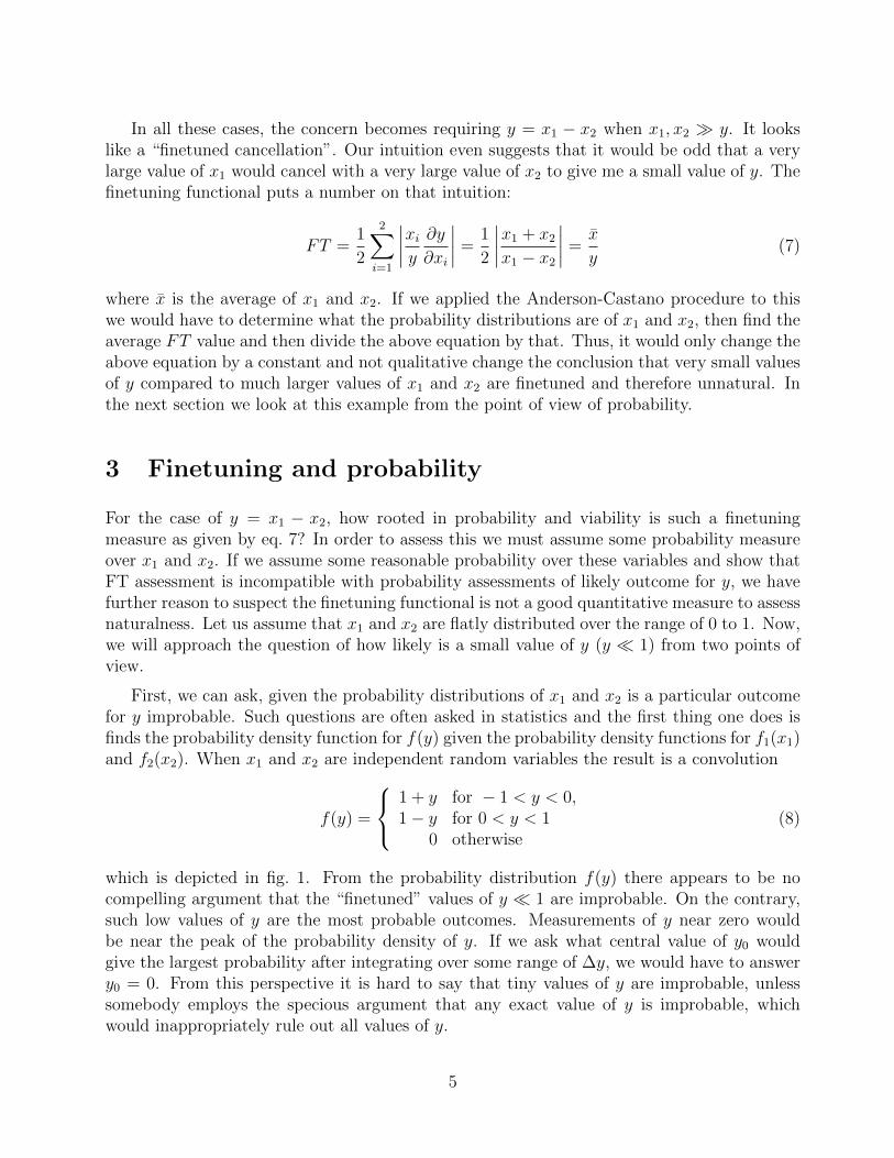
First, we can ask, given the probability distributions of x1 and x2 is a particular outcomefor y improbable. Such questions are often asked in statistics and the first thing one does isfinds the probability density function for f(y) given the probability density functions for f1(x1)and f2(x2). When x1 and x2 are independent random variables the result is a convolution

f(y) =

1 + y for − 1 < y < 0,1− y for 0 < y < 1

0 otherwise(8)

which is depicted in fig. 1. From the probability distribution f(y) there appears to be nocompelling argument that the “finetuned” values of y � 1 are improbable. On the contrary,such low values of y are the most probable outcomes. Measurements of y near zero wouldbe near the peak of the probability density of y. If we ask what central value of y0 wouldgive the largest probability after integrating over some range of ∆y, we would have to answery0 = 0. From this perspective it is hard to say that tiny values of y are improbable, unlesssomebody employs the specious argument that any exact value of y is improbable, whichwould inappropriately rule out all values of y.

5

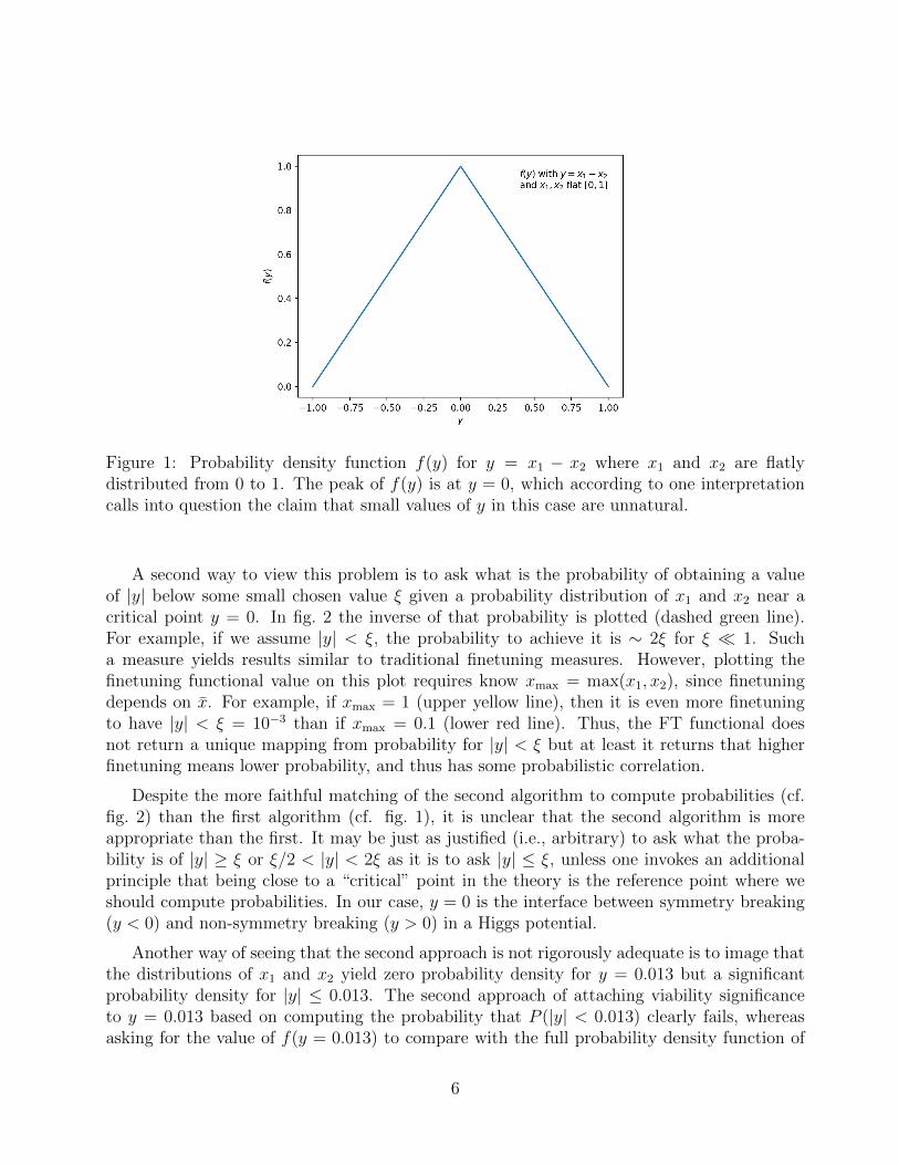
Figure 1: Probability density function f(y) for y = x1 − x2 where x1 and x2 are flatlydistributed from 0 to 1. The peak of f(y) is at y = 0, which according to one interpretationcalls into question the claim that small values of y in this case are unnatural.

A second way to view this problem is to ask what is the probability of obtaining a valueof |y| below some small chosen value ξ given a probability distribution of x1 and x2 near acritical point y = 0. In fig. 2 the inverse of that probability is plotted (dashed green line).For example, if we assume |y| < ξ, the probability to achieve it is ∼ 2ξ for ξ � 1. Sucha measure yields results similar to traditional finetuning measures. However, plotting thefinetuning functional value on this plot requires know xmax = max(x1, x2), since finetuningdepends on x. For example, if xmax = 1 (upper yellow line), then it is even more finetuningto have |y| < ξ = 10−3 than if xmax = 0.1 (lower red line). Thus, the FT functional doesnot return a unique mapping from probability for |y| < ξ but at least it returns that higherfinetuning means lower probability, and thus has some probabilistic correlation.

Despite the more faithful matching of the second algorithm to compute probabilities (cf.fig. 2) than the first algorithm (cf. fig. 1), it is unclear that the second algorithm is moreappropriate than the first. It may be just as justified (i.e., arbitrary) to ask what the proba-bility is of |y| ≥ ξ or ξ/2 < |y| < 2ξ as it is to ask |y| ≤ ξ, unless one invokes an additionalprinciple that being close to a “critical” point in the theory is the reference point where weshould compute probabilities. In our case, y = 0 is the interface between symmetry breaking(y < 0) and non-symmetry breaking (y > 0) in a Higgs potential.

Another way of seeing that the second approach is not rigorously adequate is to image thatthe distributions of x1 and x2 yield zero probability density for y = 0.013 but a significantprobability density for |y| ≤ 0.013. The second approach of attaching viability significanceto y = 0.013 based on computing the probability that P (|y| < 0.013) clearly fails, whereasasking for the value of f(y = 0.013) to compare with the full probability density function of

6

Figure 2: Finetuning computation and inverse probability of |y| < ξ when y = x1−x2 with x1and x2 flatly distributed from 0 to 1. The inverse probability of achieving very low values of|y| is correlated well, but not one-to-one, with finetuning in this example. xmax is defined to bemax(x1, x2) in the computation for finetuning. The larger the xmax the higher the finetuningto achieve low |y|.

y is defensible. However, it may only be defensible when probability is zero.

Let us return to the example earlier of the observable y depending on parameter x throughy = xn. We had stated earlier that it was nonsensical that naturalness should depend on n,and then found that Anderson-Castano rectified this problem by stating that the finetuningfunctional should be divided by the average value of finetuning. In that case, FT = 1 forall choices of x and for all choices of n. However, if we put a probability density on x andask about probability of y rather than finetuning of y, we get a very different answer. Fig. 3depicts the probability density functions fn(y) for various values of n given a flat distributionof x from 0 to 1. We see that for high powers of n the probability for lower values of y greatlyincreases. The finetuning functional does not reveal this issue.

It is interesting to revisit what we discussed above about redefining sets of observableswith respect to this specific case. If we are allowed to construct new observables yi as afunction of some canonical set of independent observables yi, as we discussed above, yi =f−1i (y1, y2, . . . , yn) we can always make a construction where FT = 1. In this specific case withy = xn, one can redefine y = y1/n and thus y = x and FT = 1. Furthermore, the probabilitydensity of y is flat from 0 to 1. This calls into question the FT measure, but it does not callinto question the probability measure. A flat probability for y is equally meaningful to assessthe viability of the theory as is the skewed and peaked probability distribution for y. However,the ability to redefine observables as functions of observables to get different FT values wouldmean loss of utility since it is not grounded in assessing probabilities.

7

Figure 3: Probability density function f(y) for y = xn for different values of n and for x flatlydistributed from 0 to 1.

4 Probability and naturalness

After considering finetuning and the criticisms of the finetuning functional as a quantita-tive means to assess naturalness, we have been led to notions of probability distributions onparameters. If naturalness has any connection to the extra-empirical judgments of theoryplausibility, which is surely what naturalness discussion is after, we have no recourse but tointroduce probability measures across parameters of the theory. A corollary to this is thatany discussion about naturalness that does not unambiguously state assumptions about theprobability distributions of parameters of the theory cannot be rooted in probability theoryand therefore has little to do with theory plausibility.

Now, any explicit claims about probability distributions of parameters is highly contro-versial, appears to go beyond the normal scientific endeavor. However, we can discuss normalscience within the language of probability distributions on parameters. For example, normaltests of a theory can be reinterpreted as an assumption of δ(xi−xthi )-function distributions onparameters, which then can be used to compute the distribution of the observables throughythi (xth1 , x

th2 , . . .). In the limit of perfect errorless theory calculation the probability distribution

of the observables would also be δ-functions: f(ythi ) = δ(yi − ythi ).

If there is theory uncertain in the calculation, e.g. from finite order perturbation theory,the δ-function distribution of parameters become a somewhat spread-out probability distri-bution for the observables, whose distribution (and therefore uncertainty) is hard to know,but the standard deviation might be estimated to be the difference in values obtained for theobservables when varying the renormalization scale by a factor of two below and above thecharacteristic energy of the observable process (e.g., mb/2 < µ < 2mb in b-meson observables

8

calculations). But that just complicates the discussion unnecessarily, so let us go back andassume that theory is perfect and we start with a δ-function distribution on parameters andobtain a δ-function distribution of observables, and we compare those observables to the data,which often Gaussian distributed.

Next, fancy statistical tests are done to see if the predictions are compatible with themeasurements, and if so the theory is said to agree with the data and the choice of parametersis then declared acceptable. One does this many times over small changes in the argumentsof the δ-function distributions on parameters and finds the full space of parameters wheretheory predictions are in agreement with observables. In the limiting case that the theoryis a valid one, and theory is calculated perfectly, and experiments yield exact results, theδ(xi − xth)-function distributions of parameters yield a δ(yi − ythi ) distribution of observablesthat exactly match the data with ythi = yexpti .

The concept of naturalness invites the theoretician to go beyond this procedure. In thelanguage above, it invites us to consider a distribution of input parameters that are not δfunctions but something more complicated with finite extent. Perhaps the parameters areflatly distributed, or Gaussian distributed, skew-distributed, or something even more compli-cated. Either way, a choice on distributions must be made or recognized somehow, and thena probability assessment on some outcome must be made. The questions then proliferate:What parameters do I attach probability distributions to? How does one determine whichprobability distributions are appropriate? What outcomes (observables, parameters?) do Icheck for probable or improbable? How is probable vs. improbable demarcated? All of thesequestions must be addressed in one form or another. Failure to do so renders any naturalnessdiscussion fuzzy with diminished meaning. At the same time, answering these questions isa highly speculative endeavor given our current understanding of quantum field theory andnature. This is what ultimately may bar naturalness from meaningful technical discourse, butit is useful to press forward to see if there are qualitative lessons one can learn about theoriesand their relative degree of probability or improbability compared to other theories.

The above discussion further begs the question of why there should be a probability distri-bution on parameters at all. Well, there is the formulation of normal science discussed abovewhich is already in terms of probability distributions on parameters, which are δ-functions.And so, a commitment to a particular distribution function has already been made implicitlyfrom this perspective. The question becomes then whether there is another distribution func-tion that is more appropriate. In Landscape discussions it is plausible that parameters are theresult of a random choice among a semi-infinite number of solutions from a more fundamentaltheory. If our universe is one random choice out of these infinite ones we certainly require thatthe probability of that choice be non-zero. That is not controversial. What becomes morecontroversial is that we might even wish to demand that the probability of our universe’schoice of outcomes be “generic.” In other words, we may wish to require that the value of thejoint probability density function over outcomes is not atypically tiny.

9

5 Probability flows of gauge couplings

We have already looked at both the finetuning interpretations and probability interpretationsof the cases y = xn and y = x1 − x2 for xi inputs and y output. One of the conclusionsfrom that discussion is that finetuning assessments might be useful for judging the plausibilityof a theory but only if they match a coherent probability interpretation, and probabilityinterpretations are only possible when distributions on parameters are specified. Let us nowproceed to investigate the IR implications of a probability distribution on a UV value of gaugecouplings.

First, let us explore the probability flow of QCD gauge coupling. We begin by assuming aflat probability distribution of MS-bar g3(MH) coupling at MH = 1015 GeV with values from0 to 0.6, chosen such that g3(Q) ≤

√4π (“finite”) down to MZ . To be clear, this is an ansatz

whose implications will be explored. For simplicity we only consider the one-loop β functionfor the renormalization group evolution of g3, which is

dg3d logQ

= − b2g33, where b =

7

8π2. (9)

The solution to this equation is

g3(Q) =g3(MH)√

1− g3(MH)2b(Q), where b(Q) = b ln(MH/Q). (10)

Note, b(Q) monotonically increases as Q flows to the IR.

Eq. 10 is analogous to our y = xn equation given earlier, where y = g3(Q) and x = g3(MH).We know (or rather posit) the distribution on x and we want to know the resulting distributionon y. Let us compute the distribution function for g3(MZ) assuming the above-stated flatdistribution on g3(MH). The probability density function is

f(g3(MZ)) =1√4π

(1 + 4π b(MZ))1/2

(1 + g3(MZ)2 b(MZ))3/2. (11)

If we had chosen g3(MH) to be flat from 0 to√

4π rather than flat from 0 to 0.6 then 83%(= 1 − 0.6/

√4π) of the probability distribution would have flowed to a divergent value of

g3(MZ). In that case the probability density function could be represented by

f ′(g3(MZ)) = 0.17 f(g3(MZ)) + 0.83 δ(g3(MZ)−√

4π) (12)

where we have let g3(MZ) =√

4π be the value of g3(MZ) where all the probability now residesfor divergent coupling. This is a complication that can be handled, but it is avoided by theoriginal assumption that g(MH) is flatly distributed from 0 to 0.6, and our probability densityfunction f(g3(MZ)) of eq. 11 holds.

As we see from fig. 4 that f(g3(MZ)) peaks at low values of g3(MZ). At first this mayseem counter-intuitive, since the g3 rises toward the infrared, and so should it not be more

10

Figure 4: The probability density function of g3(MZ) if g3(MH) at MH = 1015 GeV is assumedto be flatly distributed from 0 to

√4π.

probable to have higher values? The answer is that g3 = 0 is a fixed point (albeit unstable)of the one-loop β function and so low values of g3 in the UV stay low in the IR whereashigher values of g3 in the UV diverge rapidly in the IR. One can see this behavior by plottingprobability flow lines for g3(Q), where evenly spaced values g3(MH) are chosen to reflect itsflat distribution and then evolved down to low scales. See fig. 5. The flow lines are denserfor lower values of g3(Q) than at higher values of g3(MZ). The density of flow lines at MZ isindicative of the probability distribution of g3(MZ) at MZ . Thus, there is higher probabilityfor lower values.

How are we to interpret the flow of probability density, as defined above? It appears thatnature’s choice of g3 appears to be more probable or less probable depending on what scalewe evaluate it. A quantum field theorist might immediately recoil from this conclusion, sincewe are used to the maxim that observables (i.e., things that have meaning and a fixed valueindependent of how you might calculate them) cannot depend on what arbitrary scale youuse to conduct perturbation theory. However, we are not computing observables, and so themaxim need not apply. Nevertheless, we are left asking what scale is most appropriate to askabout the local probability density of a coupling’s value. As we discuss at the end of thissection, the resolution to this question is that the scale does not matter if we specify a finiteintegration domain. In terms of values of the couplings, RG flow will expand and contractthat finite domain at different scales but the total probability within will remain fixed.

As with most probability discussions, it is fruitful to think of betting. If a distribution isgiven at the high scale for g3(MH) and one is given a ∆g3 chip of some fixed finite range toplace at the MZ scale, what choice of position g3(MZ) would you put this chip? If one believesthat that question makes sense and there is a computable answer, which appears to be so,

11

Figure 5: Probability flow lines for the g3(Q) gauge coupling evolved from MH = 1015 GeVto MZ . Equal spacing at MH indicates flat distribution (each value equally likely in therange), whereas the converging (diverging) of flow lines at MZ indicate increased (decreased)probability density of g3(MZ) at low (high) values.

then one might be convinced of probability flows of coupling distributions from RG evolution.

We note that in normal science, where δ-function distributions are implicitly assumed forparameters, RG flow will retain δ-function distribution centered on the coupling throughoutits trajectory. Therefore, there is no conundrum to solve about what scale to evaluate acoupling’s probability – it is equally 100% probable all throughout its RG flow.

Another implication of this discussion is that a flat probability distribution of a non-abelian gauge coupling from 0 to ∞ in the UV would push an infinite number of flow linesinto a confining territory well before reaching our low value of ΛQCD and thus our theory wouldbe vanishingly improbable. Note, this conclusion could not be made by looking only at thehigh scale flat distribution, which says any value is equally likely. Only after RGE flow doesone see that the non-infinite coupling density function (where g3(Q) <

√4π by convention

here) becomes infinitesimal after RG flow into the IR. The binary probability determinationof what choices lead to too early confinement and what choices lead to QCD at Q ≤ ΛQCD iseasy to make, and in that case the realization of QCD would have infinitesimal probability.For this reason it is somewhat safe to say that if there are probability distributions on QCDcoupling they would not extend uniformly to very high values in the UV.

Repeating this exercise for a non-asymptotically free coupling, such as an abelian gaugecoupling e, one finds that the probability distribution is more peaked at the higher values ofthe coupling in the IR given a flat distribution in the UV. As we flow deeper and deeper intothe IR the probability density peaks further and further toward the maximum allowed value

12

of the coupling as a function of scale. Let us define emax(Q) to be the maximum value of e atthe scale Q given a maximum value of e at MH . If

de

d lnQ=b

2e3, with b > 0, then e2max(Q) =

e2max(MH)

1 + e2max(MH)b lnMH/Q. (13)

Also,

if emax(MH) =∞ =⇒ e2max(Q) =1

b lnMH/Q. (14)

If e(MH) is flatly distributed from 0 to emax(MH) then the probability distribution for e(Q) is

f(e(Q)) =1

emax(Q)

(1− e2max(Q)b lnMH/Q)1/2

(1− e2(Q)b lnMH/Q)3/2. (15)

where emax(Q) is given in eq. 13.

The first property to note of eq. 15 is that if emax(MH) is indeed infinite the probabilitydensity function diverges at e(Q) = emax(Q). This is because all large RG flow lines, whichwere evenly spaced in e(MH) at Q = MH , converge on emax(Q). Only a relatively small numberof lines (actually, infinitesimally small number of lines) converge to values discernably less thanemax(Q). This is because a small number of flow lines near e(MH) ∼ 1 are overwhelmed by theinfinite number of flow lines that started from e(MH)� 1. It is in this sense that we can callemax(Q) a probability flow fixed point. An implication of this discussion is that we know thata distribution with infinitely many more flow lines for e(MH)� 1 than for e(MH) ∼ 1, such asa flat distribution, could not have enabled e < emax in the IR with any reasonable probability.Thus, there is likely a firm upper bound on the distribution of abelian couplings, which isthe same conclusion we reached for non-abelian gauge couplings but for different reasons. Ofcourse, the theory becomes non-perturbative as the couplings go higher, but the qualitativemessage is similar even if the value of the emax(MH) must remain below some agreed uponperturbative bound.

These same considerations lead one to conclude that emax(Q) is a probabilistic fixed pointdeep in the IR independent of what value e started with at MH . To see this we note that theRG solution (one loop) is

e2(Q) =e2(MH)

1 + e2(MH)b lnMH/Q(16)

As Q→ 0 in the IR, the solution increasingly asymptotes to the e(Q)→ 0, but also asymptotesto emax(Q). The proper way to analyze this is to ask for some initial choice of e(MH) belowemax(MH) what value of does e(Q) have with respect to emax(Q). The answer is

e(Q)

emax(Q)=

e(MH)

emax(MH)

√1 + e2max(MH)b lnMH/Q

1 + e2(MH)b lnMH/Q. (17)

At Q = MH we have e(Q)/emax(Q) = e(MH)/emax(MH), but at Q→ 0 the expression asymp-totes to e(Q)/emax(Q) = 1. Thus, we can conclude that under high-scale flat distributions

13

abelian theories asymptote in the IR to their maximum allowed values. This conclusion holdsfor many other distributions beyond flat.

To end this section, let us remark that if we have a density function f(x) over a domaina < x < b, then we can always remap the random variable x into y by y = ψ(x) such that thedomain of y is the minimum and maximum values of ψ(x) over x’s domain a < x < b. By asuitable choice of ψ(x) one can obtain a distribution function f(y) that is arbitrarily large orsmall at y0 = ψ(x0). The implication for this is that knowing the local value of a probabilitydensity function — e.g., f(x0) — is not sufficient to know how likely it is that the value ofx is x0. We can only ask how likely it is to find x in some finite domain (x1, x2) of x-valuesenclosing x0, and equivalently how likely it is to find y in the corresponding mapped domain(ψ(x1), ψ(x2)). That is something one can place and win bets on, as discussed above. So,implicit to the above discussion is the assumption that we want to know how likely is it thatthe gauge couplings g or e falls within some small window, say g = g0 ± 0.1, or what is theprobability that the coupling is below some value g. Those are meaningful questions that canbe asked and answered in RG flows on parameter distributions at different any scale, wherethe function ψ() is the analog to RG evolution.

6 Fixed points and naturalness

The investigation into probabilistic interpretations of theories has lead us toward fixed points.Indeed, the intuitions of researchers have always been that low-energy fixed points are the mostprobable values of those couplings. This is based on an implicit assumption of underlying flatdistributions of parameters or distributions not too dissimilar from flat. Furthermore, IR fixedpoints have very low finetuning from standard finetuning functionals like those we discussedabove. Very large changes in the UV (input parameters) yield very small deviations in the IR(output parameters). However, one should caution that even in the presence of fixed pointsthere are flow lines that deviate far from the fixed point values at some non-zero IR energy,and probability distributions can be made on the UV inputs that would favor those linesand disfavor the lesser finetuned values very close to the fixed point. Nevertheless, we cantentatively hold that low finetuning may be indicative of higher probability for couplings, andtherefore higher plausibility of a theory at that point in parameter space. Again, it must beemphasized that such a conclusion is based on an implicit assumption of underlying parameterdistributions which are not too dissimilar to flat distributions, and therefore the hint of higherprobability from lower finetuning is by no means guaranteed.

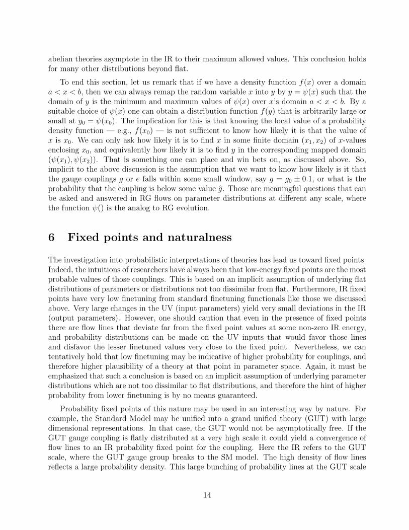
Probability fixed points of this nature may be used in an interesting way by nature. Forexample, the Standard Model may be unified into a grand unified theory (GUT) with largedimensional representations. In that case, the GUT would not be asymptotically free. If theGUT gauge coupling is flatly distributed at a very high scale it could yield a convergence offlow lines to an IR probability fixed point for the coupling. Here the IR refers to the GUTscale, where the GUT gauge group breaks to the SM model. The high density of flow linesreflects a large probability density. This large bunching of probability lines at the GUT scale

14

Figure 6: Probability flow lines for flatly distributed g3(Q) (unified coupling) at a scale of2 × 1017 GeV evolved according to a strong non-asymptotically free GUT theory down to1015 GeV and then evolved according to the Standard Model asymptotically free theory from1015 GeV down to MZ , yielding enhanced probability density at its maximum IR value.

then acts as inputs to the probability density for the SM gauge couplings. The SU(2) gaugecouplings and especially the abelian U(1)Y gauge coupling squeeze these probability flow lineseven closer together in the IR, peaking the distribution at a very narrow range. The QCDgauge coupling, since it is asymptotically free, wants to fan the probability lines out andreduce the probability density along this gmax(Q) trajectory. However, if the original densityfunction of gmax is sufficiently large at the GUT scale — the flow lines being very packed there– the fanning out process does not fully unravel the prediction and the low scale couplingis rather well peaked even for QCD. Fig. 6 depicts the scenario discussed above, where flowlines are equally spaced at a scale well above the GUT scale, and then RG flow squeezes themcloser together near the upper-limit quasi-fixed point. This could be an argument for GUTtheories not being asymptotically free.

The above discussions on gauge coupling RG flows and probabilistic interpretations issimplistic from several points of view. First, it was all done in a one-loop analysis, whichenabled us to see analytic formula for RG evolution and probability density functions. Oneshould go to higher order in RG evolution, which in realistic theories of nature will involveadditional couplings, such as the top Yukawa coupling and the Higgs coupling, albeit atsuppressed order. Nevertheless, fixed point behaviors do change especially in strongly coupledregimes due to the existence of other couplings entering the flow. Once additional couplings areadded the discussion of probability is greatly intensified. There are probability distributionsthat need to be assumed for all the parameters, and their correlations. A large joint probabilityfunction over all parameters is needed, in other words, to analyze further claims of likelihood

15

of a theory point. A line of inquiry could be to ask what distributions (beyond the obviousδ-function distributions) of high-scale parameters would yield RG flow lines that converge inthe IR to the measured values. Such theories would then be natural by definition, and likelywould involve little finetuning. However, since no theory has perfect flow to IR fixed pointbehavior, the preponderance of lines flowing to the IR fixed point neighborhood may stillnot be good enough for the strongest skeptic who would claim that an explicit probabilitydistribution is needed to make any rigorous statement at all.

7 Implications of skepticism

The critical discussion above leads to a credible skepticism to extra-empirical theory assess-ments (SEETA). We do not have a meta-theory that provides statistical distributions toparameters of theories, which is a key problem naturalness faces. It is therefore of some use topromote SEETA to a guiding principle, in apposition to naturalness and other extra-empiricalassessments. For us here, SEETA by definition is the disbelief that extra-empirical theory as-sessments, such as naturalness, enable one to find the “correct theory,” or the “more correcttheory” among competing theories. There are many resulting implications once SEETA isadopted, of which we highlight a few below.

First, since there is no meta-theory of probability distributions and any criteria to assessnaturalness, such as finetuning measures, are unacceptable to SEETA, there can be no pre-ferred regions in concordant theory space. Thus, any theory point is as good and a prioriequally likely as another. For this reason, there can be allowed no disillusionment of a theoryeven if experiment rules out a “massive fraction” of allowed parameter space, since such dec-larations implicitly assume some knowledge of probability distributions of parameters, which,however, is barred from consideration by SEETA. Therefore, as long as there is at least onetheory point that is surviving the theory is still as good as it ever was, and no judgments ofreduced plausibility can be tolerated.

A second related implication of SEETA is that only falsifiable theories allow their plau-sibility status to change, but only after discovery or after null experiments with total theorycoverage. A falsifiable theory must enable the prospect of all its theory points to be ruledout by experiment. Here we include the condition that falsifiable theories make predictionsacross its entire parameter space that have not yet been confirmed by experiment. If theentire parameter space of the theory can be covered, then a falsifiable theory will either beruled out because nothing new is found, or it is established beyond the standard theory sincea non-trivial prediction was borne out by experiment.

Now, the subtlety with this second implication is that one can extract out of any testabletheory a falsifiable theory. For example, I may have a theory T (e.g., supersymmetry), whichhas two regions of parameter space TF and TNF , where T = TF ⊕ TNF. One region, TF , isthe area that makes new predictions and can be non-trivially tested by experiment in thereasonable future (e.g., very low energy minimal supersymmetry). Another region, TNF, is theregion of parameter space that is not TF. If a theory T has TF 6= ∅ then the theory is testable,

16

and if TNF = ∅ it is falsifiable. If TNF 6= ∅ then one can declare a new theory T ′ which is theprojection PF of the falsifiable region TF:

T ′ = PF(T ) = PF(TF ⊕ TNF) = TF. (18)

T ′ is a falsifiable theory, albeit artificially created, and its plausibility status is guaranteedto change after experimental inquiry. An example of this is projecting all of supersymmetry(T ) down to a very minimal supersymmetric SU(5) GUT with low-scale supersymmetry (TF),which is falsifiable and indeed was falsified [15].

The difficulty with such falsifiable projections is the sometimes artificial nature of thedivision between TF and TNF. The separation between the two is sometimes made not out oftheory considerations, in contrast to the SU(5) supersymmetric GUT example given above,but rather the perceived boundaries to what experiments are willing and able to achieve inthe near term. For example, if T is supersymmetry, and TF is what the LHC can find, thenthere is a tendency to misname T ′ = PF(T ) = TF as “supersymmetry”, and when it is notfound, it is said that “supersymmetry” has been ruled out. In reality, T ′ is better called“LHC-projected supersymmetry”, and therefore the LHC is capable of ruling out only “LHC-projected supersymmetry”, and not “supersymmetry,” if it is not found. Projecting T ontoTF to form a falsifiable T ′ based only on recognizing what experiment can and cannot do inthe near term creates artificial theories whose falsification is not very meaningful.

Finally, a third implication of SEETA is that theory preference then becomes not aboutwhat theory is more likely to be correct but what theory is practically more advantageousor wanted for other reasons. Such reasons include fewer parameters, easier to calculate, hasnew experimental signatures to pursue, interesting connections to other subfields of physics,mathematical interest, etc. There are many reasons to prefer theories beyond one being morecorrect than another — the only attitude unacceptable to SEETA is to say that one theoryis more “correct” or more likely to be correct than another theory that is equally empiricallyadequate. No theory of theory preference will be given here, except to say that “diversity”has a strong claim to a quality for preference. If theorists only develop and analyze theoriesthat give the same phenomena, at the expense of exploring other theories equally compatiblewith experiment, there becomes the practical problem of not arguing for or analyzing newsignals requiring new experiments. A few examples out of many in the literature that havethe quality of diversity at least going for it are clockwork theories [16, 17] and theories ofsuperlight dark matter (see, e.g., [18, 19]). These theories lead to new experiments, or newexperimental analyses, that may not have been performed otherwise.

To conclude and summarize the skeptical ethos: theories must be compatible with experi-ment, and any that are should be viewed as just as likely as any others. There is no concept ofa theory being “almost ruled out” when its parameter space shrinks due to null experimentalresults, since such descriptions imply knowledge of as-yet unknown probability distributionsof parameters. Regarding naturalness, it becomes a theory quality upon a well-defined al-gorithm to quantify it. Without yet having a meta-theory of probability distributions overparameters, one must abandon standard naturalness as a quality that points to theories thatare more likely to be correct, which may be fatal for naturalness since that is implicitly its

17

main raison d’etre. It is important, nevertheless, to continue to assess theories beyond theirempirical adequacy. Seeking diversity is one example of a potentially fruitful extra-empiricalcriterion. Other qualities such as simplicity, calculability, consilience, etc., may also be use-ful practical qualities to declare preferred theories. However, as argued, there is no knownguaranteed justification to call these preferred theories more correct.

Acknowledgments: I am grateful for discussions with A. Hebecker, S. Martin, A. Pierce, andY. Zhao. This work was supported in part by the DOE under grant DE-SC0007859.

References

[1] J.D. Wells. “Lexicon of Theory Qualities.” Physics Resource Manuscripts (19 June 2018).http://umich.edu/~jwells/prms/prm8.pdf

[2] C. Patrignani et al. (Particle Data Group), Chin. Phys. C, 40, 100001 (2016) and 2017update.

[3] G. F. Giudice, “Naturally Speaking: The Naturalness Criterion and Physics at the LHC,”[arXiv:0801.2562 [hep-ph]].

[4] M. Farina, D. Pappadopulo and A. Strumia, “A modified naturalness principleand its experimental tests,” JHEP 1308, 022 (2013) doi:10.1007/JHEP08(2013)022[arXiv:1303.7244 [hep-ph]].

[5] G. Marques Tavares, M. Schmaltz and W. Skiba, “Higgs mass naturalness and scale invari-ance in the UV,” Phys. Rev. D 89, no. 1, 015009 (2014) doi:10.1103/PhysRevD.89.015009[arXiv:1308.0025 [hep-ph]].

[6] A. de Gouvea, D. Hernandez and T. M. P. Tait, “Criteria for Natural Hierarchies,” Phys.Rev. D 89, no. 11, 115005 (2014) doi:10.1103/PhysRevD.89.115005 [arXiv:1402.2658[hep-ph]].

[7] P. Williams, “Naturalness, the autonomy of scales, and the 125 GeV Higgs,” Stud. Hist.Phil. Sci. B 51, 82 (2015). doi:10.1016/j.shpsb.2015.05.003

[8] J. D. Wells, “Higgs naturalness and the scalar boson proliferation instability problem,”Synthese 194, no. 2, 477 (2017) doi:10.1007/s11229-014-0618-8 [arXiv:1603.06131 [hep-ph]].

[9] G. F. Giudice, “The Dawn of the Post-Naturalness Era,” arXiv:1710.07663 [physics.hist-ph].

[10] J. R. Ellis, K. Enqvist, D. V. Nanopoulos and F. Zwirner, “Observables in Low-EnergySuperstring Models,” Mod. Phys. Lett. A 1, 57 (1986). doi:10.1142/S0217732386000105

18

[11] R. Barbieri and G. F. Giudice, “Upper Bounds on Supersymmetric Particle Masses,”Nucl. Phys. B 306, 63 (1988). doi:10.1016/0550-3213(88)90171-X

[12] G. W. Anderson and D. J. Castano, “Measures of fine tuning,” Phys. Lett. B 347, 300(1995) doi:10.1016/0370-2693(95)00051-L [hep-ph/9409419].

[13] G. W. Anderson and D. J. Castano, “Naturalness and superpartner masses orwhen to give up on weak scale supersymmetry,” Phys. Rev. D 52, 1693 (1995)doi:10.1103/PhysRevD.52.1693 [hep-ph/9412322].

[14] S. P. Martin, “A Supersymmetry primer,” Adv. Ser. Direct. High EnergyPhys. 21, 1 (2010) [Adv. Ser. Direct. High Energy Phys. 18, 1 (1998)]doi:10.1142/9789812839657 0001, 10.1142/9789814307505 0001 [hep-ph/9709356]. Ver-sion 7 from January 27, 2016.

[15] H. Murayama and A. Pierce, “Not even decoupling can save minimal supersymmet-ric SU(5),” Phys. Rev. D 65, 055009 (2002) doi:10.1103/PhysRevD.65.055009 [hep-ph/0108104].

[16] G. F. Giudice and M. McCullough, “A Clockwork Theory,” JHEP 1702, 036 (2017)doi:10.1007/JHEP02(2017)036 [arXiv:1610.07962 [hep-ph]].

[17] G. F. Giudice, Y. Kats, M. McCullough, R. Torre and A. Urbano, “Clock-work/linear dilaton: structure and phenomenology,” JHEP 1806, 009 (2018)doi:10.1007/JHEP06(2018)009 [arXiv:1711.08437 [hep-ph]].

[18] Y. Hochberg, Y. Zhao and K. M. Zurek, “Superconducting Detectors for Superlight DarkMatter,” Phys. Rev. Lett. 116, no. 1, 011301 (2016) doi:10.1103/PhysRevLett.116.011301[arXiv:1504.07237 [hep-ph]].

[19] Y. Hochberg, M. Pyle, Y. Zhao and K. M. Zurek, “Detecting Superlight Dark Matter withFermi-Degenerate Materials,” JHEP 1608, 057 (2016) doi:10.1007/JHEP08(2016)057[arXiv:1512.04533 [hep-ph]].

19