nature protocols: doi:10.1038/nprot.2017 · peel off the tape and use a pair of tweezers to tear...
TRANSCRIPT
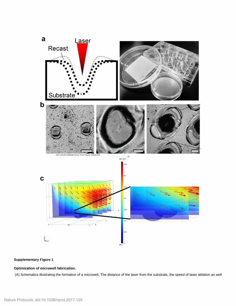
Supplementary Figure 1
Optimization of microwell fabrication.
(A) Schematics illustrating the formation of a microwell. The distance of the laser from the substrate, the speed of laser ablation as well
Nature Protocols: doi:10.1038/nprot.2017.125

as laser power affects the depth and width of microwell formed. The higher the laser power, the deeper and wider the resultant microwell becomes. The layer of the recast is an artifact generated by the laser process, which becomes prominent with stronger laser power. (B) Phase contrast images of the smallest (left; average inner diameter 50 µm; Scale bar is 50 µm) and largest possible microwell that can be fabricated (middle; average inner diameter 341.5 µm; Scale bar is 100 µm.) with laser-ablation. (Right) Magnified view of the array of microwells with optimal parameters. (C) Simulation results of flow velocity at the entrance of the channel. (left) Cross-sectional slices of the velocity magnitude in the XZ-plane. Coloured scale bar represents the velocity magnitude in mm/s. Red arrows depict the direction of the flow and have lengths that are proportional to the velocity magnitude. (right) Zoomed in view of the panel a where the microwells are. The uniform dark blue colour within the microwells indicate that there is no flow in that region i.e. cells in culture do not experience shear stresses from the flow of fluid entering the channel from the gradient generator.
Nature Protocols: doi:10.1038/nprot.2017.125

Supplementary Figure 2
Optimization of microwell parameters.
Phase contrast images of cancer cells seeded into microwells of different average diameters (~107 µm, 187.5 µm and 341.5 µm from left to right). Images were obtained with a 20X objective lens. Scale bar is 50 µm.
Nature Protocols: doi:10.1038/nprot.2017.125

Supplementary Figure 3
Custom tapered microwells for CTC cluster formation.
Clinical samples do not form clusters in conventional round bottom wells (left) but are able to develop clusters consistently in our tapered microwell assay. These clusters can be formed in microwells generated by either laser-ablation (middle) or microfabrication (right).
Nature Protocols: doi:10.1038/nprot.2017.125

Supplementary Figure 4
Nature Protocols: doi:10.1038/nprot.2017.125

Step 79: Enumeration of cell counts in a fixed area reveal cell packing density.
(a) Cell counts in a fixed area (e.g. 50 µm by 50 µm) are obtained from images of cultures with WBCs from healthy volunteer only and spiked cultures with WBC and cancer cell lines. (b) Spiked cultures start to form aggregates of higher cell density (> 8 cells per 2500 µm
2) after only 3 days in culture.
Nature Protocols: doi:10.1038/nprot.2017.125

Supplementary Figure 5
Substrate adherence requirement.
(a) Surfactant treatment of polystyrene surfaces is temporary, and spheroids of cell lines cultured in laser-ablated microwells dispersed after three days in culture. N=3. Scale bar is 50 µm. (b) Clinical samples can form loose clusters with microwells of 187.5 µm average diameter in the absence of surfactant treatment. N=3. Scale bar is 50 µm.
Nature Protocols: doi:10.1038/nprot.2017.125
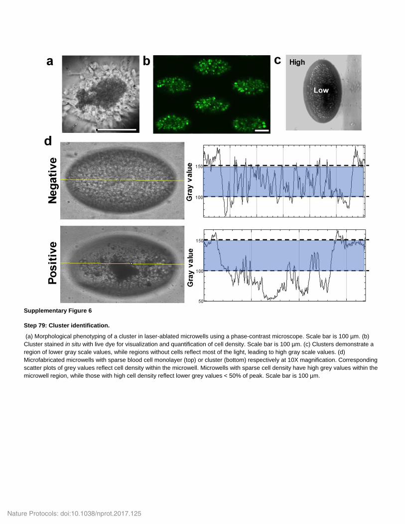
Supplementary Figure 6
Step 79: Cluster identification.
(a) Morphological phenotyping of a cluster in laser-ablated microwells using a phase-contrast microscope. Scale bar is 100 µm. (b)
Cluster stained in situ with live dye for visualization and quantification of cell density. Scale bar is 100 µm. (c) Clusters demonstrate a
region of lower gray scale values, while regions without cells reflect most of the light, leading to high gray scale values. (d)
Microfabricated microwells with sparse blood cell monolayer (top) or cluster (bottom) respectively at 10X magnification. Corresponding
scatter plots of grey values reflect cell density within the microwell. Microwells with sparse cell density have high grey values within the
microwell region, while those with high cell density reflect lower grey values < 50% of peak. Scale bar is 100 µm.
Nature Protocols: doi:10.1038/nprot.2017.125

Supplementary Figure 7
Panel of healthy sample cultures.
Cultures of healthy blood samples demonstrate either cell debris (25%) or monolayer of residual blood cells (75%) (n=16). Scale bar is 50 µm.
Nature Protocols: doi:10.1038/nprot.2017.125

Supplementary Figure 8
Step 6: Fabrication of the primary mold with elliptical pillars.
(a) The 4” soda lime mask with the elliptical opening patterned in the Cr layer, already coated with the 500-nm thick PMGI sacrificial layer (step 28). (b) SU-8 spin coating of the mask plate. SU-8 3050 is poured carefully on the plate while this is placed on the vacuum chuck of the spin coater (steps 29 and 31). (c) Soft baking of the SU-8 (steps 30 and 32). (d) Loading of the mask (face down) in the UV exposure system. A blank mask plate is placed face up to prevent reflection of the UV light from the bottom, after passing through the SU-8 layer. (e) The opal diffuser is placed on top of the mask (step 33). (f) Development of the mask. When all the unexposed SU-8 has been removed, the plate is cleaned with spraying SU-8 developer first and IPA later, and then dried with gentle nitrogen flow (step 35).
Nature Protocols: doi:10.1038/nprot.2017.125

Supplementary Figure 9
Step 34: Soft-lithographic replica of the primary mold.
(a) The mask plate with the SU-8 dome-shaped pillars is placed in a petri dish face up (Step 39). (b) PDMS is poured on the mask (step 40). (c) De-gassing of the PDMS to remove all trapped air. (d) After curing, the PDMS is cut along the mask border with a razor blade (step 43). (e) Using a pair of tweezer, the cured PDMS is gently peeled off from the mask. (f) PDMS replica and original mold after the peeling-off step is completed.
Nature Protocols: doi:10.1038/nprot.2017.125

Supplementary Figure 10
Step 37: The soft-lithographic replica of the secondary mold.
(a) Surface activation of the PDMS Secondary mold using oxygen plasma (step 45). (b) The activated PDMS secondary mold is placed in a vacuum jar along with a small quantity of silane for its silanization process (step 45). (c) After the silanization is completed, the Secondary Mold is placed in a petri dish and fresh uncured PDMS is poured (same as in previous image and step 39-40 and 48). Then, after curing the PDMS is cut along the Secondary Mold border with a razor blade (as in step 48) and the replica is gently peeled off. (d) Secondary Mold (right) and its PDMS replica (left)
Nature Protocols: doi:10.1038/nprot.2017.125

Supplementary Figure 11
Step 48: Release of PDMS from the mold after curing.
(a) Carefully cut out the PDMS without cutting the SU-8 pattern of the gradient generator. (b) Slide the blade along the inner wall of the aluminum mold for the barrier layer. (c) Cut along the outline of the PDMS replica mold of the microwell layer drawn in Step 50. (d-f) Use the blade to lift the corners of the PDMS from each of the three molds. (g-i) Peel out the gradient generator, barrier and microwell layers from their respective molds.
Nature Protocols: doi:10.1038/nprot.2017.125

Supplementary Figure 12
Steps 49 and 50: Preparation of each PDMS layer prior to assembly.
(a) Trim the sides of the gradient generator and punch two vertical holes at the inlets. (b) Cover the top surface of the barrier layer with tape. (c) Flip the barrier layer upside down and cut through the thin layer of PDMS along the length on both sides of each channel. (d) Peel off the tape and use a pair of tweezers to tear out the thin strips of PDMS. (e, f) Place the microwell layer under the barrier layer and align it with the channels in the barrier layer. Trim off the sides of the microwell layer using the edges of the barrier layer as a guide.
Nature Protocols: doi:10.1038/nprot.2017.125
Supplementary Tutorial 1: COMSOL Tutorial for Simulating Flow Rates and
Concentration Gradient
1. Create a new model.
2. Select 2D Space Dimension and click “next”.
3. Under “Add Physics”, select Fluid Flow > Single Phase Flow > Laminar Flow (spf) > +
for simulating flow rates in the device.
4. For simulating concentration gradients, select Chemical Species Transport > Transport of
Diluted Species (chds) > +.
5. Click “next”.
6. Select “Stationary” study and click “finish”.
Nature Protocols: doi:10.1038/nprot.2017.125

7. Select "Geometry 1" on the Model Builder Panel. Change the Length unit to mm.
8. Right click "Geometry 1" on the Model Builder Panel and select the "Import" option.
9. Browse the file to import and click "Import".
Nature Protocols: doi:10.1038/nprot.2017.125

10. Right click "Geometry 1" on the Model Builder Panel and select the "Delete Entities"
option.
11. Under Geometric entity level, select "Domain" and select all the regions in the
imported drawing to be removed.
12. Select “Build all”.
Nature Protocols: doi:10.1038/nprot.2017.125

13. Right click "Materials" on the Model Builder Panel and select the "Open Material
Browser" option.
14. Under “Material Browser”, select Material Library> Simple Oxides > H20(water) and
select liquid phase. Add Material to Model.
Nature Protocols: doi:10.1038/nprot.2017.125

15. Right click "Laminar Flow" on the Model Builder Panel and select the "+ Inlet" and"
+ Outlet" options.
16. Select "Inlet 1" on the Model Builder Panel. Select the boundaries for the inlets and
input the normal inflow velocity (hold the scroll button on the mouse to zoom in and out,
right click to drag the model around). This value can be calculated by dividing the flow rate
(50µl/min) by the cross sectional area of the inlet channel (50µm x 50µm) and further
dividing by 60 (to convert min to s).
Nature Protocols: doi:10.1038/nprot.2017.125

17. Click "Outlet 1" on the Model Builder Panel. Add the boundaries for the outlets.
18. Right click "Laminar Flow" on the Model Builder Panel and select "+ Inflow" twice
and" + Outflow" eight times (2 inlets and 8 outlets).
Nature Protocols: doi:10.1038/nprot.2017.125

19. Select "Convection and Diffusion 1" on the Model Builder Panel. Under Velocity
field, select "Velocity field (Spf/fp1)". Next, select "H2O(water)[liquid]" under Bulk material.
Finally, define Dc as 1e-4.
20. Select "Inflow 1" on the Model Builder Panel. Select the boundary for the inlet and
input the concentration as 0.
21. Select "Inflow 2" on the Model Builder Panel. Select the boundary for the inlet and
input the concentration as 1000.
Nature Protocols: doi:10.1038/nprot.2017.125

22. Click "Outflow 1" on the Model Builder Panel. Add the boundaries for the outlet first
outlet. Repeat this step for all 8 outflows.
23. Select "Mesh 1" on the Model Builder Panel and select the "Finer" Element size.
Click “Build All”.
24. Right click "Device Simulation.mph (root)" on the Model Builder Panel and select
"Add Study". Select “Stationary” study type.
Nature Protocols: doi:10.1038/nprot.2017.125
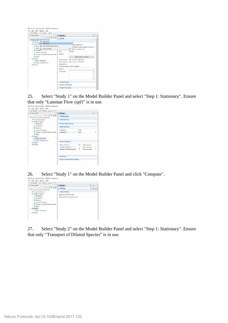
25. Select "Study 1" on the Model Builder Panel and select "Step 1: Stationary". Ensure
that only “Laminar Flow (spf)” is in use.
26. Select "Study 1" on the Model Builder Panel and click "Compute".
27. Select "Study 2" on the Model Builder Panel and select "Step 1: Stationary". Ensure
that only “Transport of Diluted Species” is in use.
Nature Protocols: doi:10.1038/nprot.2017.125

28. Select "Study 2" on the Model Builder Panel and click "Compute".
29. 2D plot groups for Velocity, Pressure and Concentration are plotted automatically.
To plot 1D plots to compare the flow velocity at each outlet, click “Results” on the Model
Builder Panel. Right click “Data Sets” and select “+ Cut Line 2D”. Select Solution 1 and
fill in the parameters as shown. Click Plot.
Nature Protocols: doi:10.1038/nprot.2017.125

Nature Protocols: doi:10.1038/nprot.2017.125

30. To also plot 1D plots to compare the fluid concentrations at each outlet, click “Results”
on the Model Builder Panel. Right click “Data Sets” and select “+ Cut Line 2D”. Select
Solution 2 and fill in the parameters as shown. Click Plot.
31. Right click "Results" on the Model Builder Panel and select the "+ 1D Plot Group"
option twice to plot the velocity and concentration.
32. Right click "1D Plot Group 1" on the Model Builder Panel and select the "+ Line
Graph" option. Do the same for "1D Plot Group 2".
Nature Protocols: doi:10.1038/nprot.2017.125

33. Select “Line Graph 1” under “1D Plot Group 1”. Select “Cut Line 2D 1” under Data
set. Ensure that the expression is as shown for plotting velocity. Click “Plot”.
34. To plot the concentration, select “1D Plot Group 2” and select “Solution 2”. Click
“Plot”. Select “Line Graph 1” under “1D Plot Group 2”. Select “Cut Line 2D 2” under Data
set. Click on the green and orange triangles followed by the expression to plot. Click Plot.
Nature Protocols: doi:10.1038/nprot.2017.125

35. To export data, right click on a plot and select “+ Add Plot Data to Export”.
Thereafter, browse a location to save the file as well as indicate the data format.
Nature Protocols: doi:10.1038/nprot.2017.125