naval postgraduate school · author amanda r. mueller 7. performing organization name(s) and...

NAVAL POSTGRADUATE

SCHOOL

MONTEREY, CALIFORNIA

THESIS

Approved for public release; distribution is unlimited

LIDAR AND IMAGE POINT CLOUD COMPARISON

by

Amanda R. Mueller

September 2014

Thesis Advisor: Richard C. Olsen Second Reader: David M. Trask

THIS PAGE INTENTIONALLY LEFT BLANK

i

REPORT DOCUMENTATION PAGE Form Approved OMB No. 0704-0188 Public reporting burden for this collection of information is estimated to average 1 hour per response, including the time for reviewing instruction, searching existing data sources, gathering and maintaining the data needed, and completing and reviewing the collection of information. Send comments regarding this burden estimate or any other aspect of this collection of information, including suggestions for reducing this burden, to Washington headquarters Services, Directorate for Information Operations and Reports, 1215 Jefferson Davis Highway, Suite 1204, Arlington, VA 22202-4302, and to the Office of Management and Budget, Paperwork Reduction Project (0704-0188) Washington DC 20503.

1. AGENCY USE ONLY (Leave blank)

2. REPORT DATE September 2014

3. REPORT TYPE AND DATES COVERED Master’s Thesis

4. TITLE AND SUBTITLE LIDAR AND IMAGE POINT CLOUD COMPARISON

5. FUNDING NUMBERS

6. AUTHOR Amanda R. Mueller

7. PERFORMING ORGANIZATION NAME(S) AND ADDRESS(ES) Naval Postgraduate School Monterey, CA 93943-5000

8. PERFORMING ORGANIZATION REPORT NUMBER

9. SPONSORING /MONITORING AGENCY NAME(S) AND ADDRESS(ES) N/A

10. SPONSORING/MONITORING AGENCY REPORT NUMBER

11. SUPPLEMENTARY NOTES The views expressed in this thesis are those of the author and do not reflect the official policy or position of the Department of Defense or the U.S. Government. IRB protocol number ____N/A____.

12a. DISTRIBUTION / AVAILABILITY STATEMENT Approved for public release; distribution is unlimited

12b. DISTRIBUTION CODE A

13. ABSTRACT (maximum 200 words)

This paper analyzes new techniques used to extract 3D point clouds from airborne and satellite electro-optical data. The objective of this research was to compare the three types of point clouds to determine whether image point clouds could compete with the accuracy of LiDAR point clouds. The two main types of image point clouds are those created photogrammetrically, with two side-by-side images, or through feature matching between multiple images using multiview stereo techniques. Two software packages known for handling aerial imagery, IMAGINE Photogrammetry and Agisoft Photoscan Pro, were used to create such models. They were also tested with sub-meter resolution satellite imagery to determine whether much larger, but still truthful, models could be produced. It was found that neither software package is equipped to vertically analyze satellite imagery but both were successful when applied to aerial imagery. The photogrammetry model contained fewer points than the multiview model but maintained building shape better. While the photogrammetry model was determined to be the more accurate of the two it still did not compare to the accuracy of the LiDAR data.

14. SUBJECT TERMS LiDAR, photogrammetry, multiview stereo, point cloud 15. NUMBER OF

PAGES 83

16. PRICE CODE

17. SECURITY CLASSIFICATION OF REPORT

Unclassified

18. SECURITY CLASSIFICATION OF THIS PAGE

Unclassified

19. SECURITY CLASSIFICATION OF ABSTRACT

Unclassified

20. LIMITATION OF ABSTRACT

UU

NSN 7540-01-280-5500 Standard Form 298 (Rev. 2-89) Prescribed by ANSI Std. 239-18

ii


iii

Approved for public release; distribution is unlimited

LIDAR AND IMAGE POINT CLOUD COMPARISON

Amanda R. Mueller Second Lieutenant, United States Air Force

B.S., United States Air Force Academy, 2013

Submitted in partial fulfillment of the requirements for the degree of

MASTER OF SCIENCE IN REMOTE SENSING INTELLIGENCE

from the

NAVAL POSTGRADUATE SCHOOL September 2014

Author: Amanda R. Mueller

Approved by: Richard C. Olsen Thesis Advisor

David M. Trask Second Reader

Dan C. Boger Chair, Department of Information Science

iv


v

ABSTRACT

This paper analyzes new techniques used to extract 3D point clouds from airborne and

satellite electro-optical data. The objective of this research was to compare the three types

of point clouds to determine whether image point clouds could compete with the

accuracy of LiDAR point clouds. The two main types of image point clouds are those

created photogrammetrically, with two side-by-side images, or through feature matching

between multiple images using multiview stereo techniques. Two software packages

known for handling aerial imagery, IMAGINE Photogrammetry and Agisoft Photoscan

Pro, were used to create such models. They were also tested with sub-meter resolution

satellite imagery to determine whether much larger, but still truthful, models could be

produced. It was found that neither software package is equipped to vertically analyze

satellite imagery but both were successful when applied to aerial imagery. The

photogrammetry model contained fewer points than the multiview model but maintained

building shape better. While the photogrammetry model was determined to be the more

accurate of the two it still did not compare to the accuracy of the LiDAR data.

vi


vii

TABLE OF CONTENTS

I. INTRODUCTION........................................................................................................1 A. PURPOSE OF RESEARCH ...........................................................................1 B. OBJECTIVE ....................................................................................................1

II. BACKGROUND ..........................................................................................................3 A. PHOTOGRAMMETRY ..................................................................................3

1. Mechanics behind Photogrammetry ................................................12 2. Computer Photogrammetry and MVS ............................................13 3. How It Works .....................................................................................17

B. LIDAR BACKGROUND ..............................................................................19 1. Physics of LiDAR Systems ................................................................20

III. DATA AND SOFTWARE .........................................................................................23 A. LIDAR AND IMAGERY OF NPS ...............................................................23 B. AIRBORNE DATA ........................................................................................25 C. SATELLITE DATA.......................................................................................27 D. SOFTWARE ...................................................................................................28

IV. PROCESSING, RESULTS, AND ANALYSIS .......................................................29 A. AERIAL IMAGERY MULTIVIEW STEREO ..........................................29

1. Trial #1 ................................................................................................29 2. Trial #2 ................................................................................................34 3. Trial #3 ................................................................................................35

B. SATELLITE IMAGERY MULTIVIEW STEREO ...................................38 C. PHOTOGRAMMETRIC MODELS ............................................................41

1. Aerial Imagery ...................................................................................42 2. Satellite Imagery ................................................................................45

D. COMPARISON WITH LIDAR....................................................................47 1. Aerial ...................................................................................................48 2. Satellite ................................................................................................52

V. SUMMARY AND CONCLUSION ..........................................................................59

LIST OF REFERENCES ......................................................................................................61

INITIAL DISTRIBUTION LIST .........................................................................................65

viii


ix

LIST OF FIGURES

Figure 1. “Plan of the Village of Buc, near Versailles” Created by Aimé Laussedat in 1861 (from Laussedat, 1899, p. 54) ...............................................................4

Figure 2. Hot Air Balloon Photography of Paris taken by Gaspard-Felix Tournachon, Better Known as Nadar (from Saiz, 2012) ...................................5

Figure 3. Schematic of the Scheimpflug Principle (from Erdkamp, 2011) .......................6 Figure 4. Scheimpflug’s Camera Configurations (from Erdkamp, 2011) .........................7 Figure 5. Scheimpflug’s Photo Perspektograph Model II (from Erdkamp, 2011) ............8 Figure 6. Topographic Survey of Ostia from a Hot Air Balloon (from Shepherd,

2006) ..................................................................................................................9 Figure 7. Mosaic of Images Taken of Ostia For Use in the Topographic Survey by

Hot Air Balloon (from Shepherd, 2006) ..........................................................10 Figure 8. Three-Lens Camera Used by USGS Team in Alaska, with One Vertical

and Two Obliques (from “Early Techniques,” 2000) ......................................11 Figure 9. Scanning Stereoscope (from “Old Delft,” 2009) .............................................12 Figure 10. Quam Differenced Two Images from the 1969 Mariner Mission to Mars as

a Form of Change Detection (from Quam, 1971, p. 77) ..................................14 Figure 11. Block Diagram Illustrating Relationships between Image-to-Model

Techniques .......................................................................................................17 Figure 12. Deriving Depths of Points P and Q using Two Images (from “Image-

based Measurements,” 2008) ...........................................................................18 Figure 13. Electronic Total Stations Measure Heights of Unreachable Objects Via

Remote Elevation Measurement (from “Total Station,” n.d.) .........................19 Figure 14. Main Components of Airborne LiDAR (from Diaz, 2011) .............................21 Figure 15. LiDAR Dataset of the NPS Campus East of the Monterey Peninsula (map

from Google Maps, n.d.) ..................................................................................23 Figure 16. LiDAR Dataset Compared to a Photograph of Hermann Hall (from “NPS

Statistics,” 2014) ..............................................................................................24 Figure 17. Close-up Near-nadir View of Glasgow Hall Aerial Imagery ..........................25 Figure 18. WSI Image Subset to Glasgow Hall and Dudley Knox Library ......................30 Figure 19. Three Aligned Photos (One Off-screen) and Sparse Point Cloud ...................31 Figure 20. Sparse and Dense Aerial Point Clouds in Agisoft ...........................................32 Figure 21. IMAGINE Photogrammetry’s Point Measurement Window ..........................43 Figure 22. GCPs and Tie Points in IMAGINE Photogrammetry ......................................44 Figure 23. Photogrammetry Point Cloud of Glasgow Hall, Aerial Imagery .....................45 Figure 24. Stereo Photogrammetry Point Cloud of Monterey, CA; Horizontal View of

the Southern Edge (Top), Topographic Map (Left, after “Digital Wisdom,” 2014), Nadir View (Bottom) ...........................................................................47

Figure 25. Transects of Glasgow Hall Models Using Aerial Imagery, Top: Northwest to Southeast, Bottom: Southwest to Northeast ................................................52

Figure 26. Aerial Photogrammetry Model of Monterey, Clipped to NPS ........................53 Figure 27. MVS Satellite Model of Monterey, Clipped to NPS .......................................53 Figure 28. Close-up of Satellite Photogrammetry Model with LiDAR of NPS ...............55

x

Figure 29. Close-up of Satellite MVS Model with LiDAR of NPS ..................................55 Figure 30. Horizontal View of Satellite Photogrammetry Model with LiDAR of NPS ...56 Figure 31. Horizontal View of Satellite MVS Model with LiDAR of NPS .....................56 Figure 32. Transects of Glasgow Hall Models Using Satellite Imagery, Top:

Northwest to Southeast, Bottom: Southwest to Northeast ...............................57

xi

LIST OF TABLES

Table 1. Comparison of October 2013 and May 2014 Hasselblad Imagery (Oriented Roughly North-South) .....................................................................26

Table 2. UltraCam Eagle Imagery of Glasgow Hall ......................................................26 Table 3. Satellite Imagery Thumbnails, Date of Collection, Run Number, and

Details (after Digital Globe, 2013) ..................................................................27 Table 4. Dense Points Clouds for Trials Utilizing All Three Datasets ..........................33 Table 5. Models of Each Six-Image Collection Compared to Winning Combined

Model, Using Aerial Imagery ..........................................................................34 Table 6. Comparison of WSI Models ............................................................................35 Table 7. WSI Models of Five and Six Images ...............................................................37 Table 8. Order Satellite Images were added to Agisoft Photoscan Pro .........................38 Table 9. Five Successive MVS Runs, Adding One New Satellite Image Each Time ...39 Table 10. Satellite MVS Close-up of NPS .......................................................................40 Table 11. Side-view of Satellite MVS Models, Indicating Z-Errors ...............................41 Table 12. Comparing Imagery Results to LiDAR Ground Truth (View of Glasgow

Hall from the Southwest) .................................................................................49 Table 13. Comparing Imagery Results to LiDAR Ground Truth (View of Glasgow

Hall from the Northeast) ..................................................................................50

xii


xiii

LIST OF ACRONYMS AND ABBREVIATIONS

2D 2-dimensional

2.5D 2.5-dimensional

3D 3-dimensional

CC CloudCompare

DEM digital elevation model

DSM digital surface model

ETS electronic total station

GCP ground control point

GPS Global Positioning System

IMU inertial measurements unit

LiDAR light detection and ranging

MI mutual information

MVS multiview stereo

PRF pulse repetition frequency

QTM Quick Terrain Modeler

SfM structure from motion

TIN triangular irregular network

TOF time of flight

UAV unmanned aerial vehicle

USGS United States Geological Survey

UTM Universal Transverse Mercator

WGS 84 World Geodetic System 1984

WSI Watershed Sciences, Inc.

xiv


xv

ACKNOWLEDGMENTS

I would like to thank all of the members of the NPS Remote Sensing Center who

let me pick their brains this past year: Scott Runyon, Sarah Richter, Chelsea Esterline,

Jean Ferreira, and Andre Jalobeanu. Additional thanks go to Jeremy Metcalf for sharing

his Agisoft expertise, Angie Kim for learning Imagine with me and taking turns on the

computer, and Colonel Dave Trask for agreeing to take the time to read every last page of

my thesis.

I would also like to acknowledge professors Chris Olsen and Fred Kruse for

voluntarily dedicating so many hours of their time to me and my classmate. Whether it

meant hiking over to Glasgow or up to the fourth floor, we both appreciated the time and

effort you spent on us. And speaking of my classmate, I would like to thank Shelli Cone,

not only for being a great sounding board as I brainstormed my thesis, but for all of the

other little things this year. Thanks for rides to the airport, introducing me to people in

Monterey, studying for finals with me, teaching me how to cook, and on and on. I was so

happy the Navy decided at the last minute to allow me a classmate, but I am even happier

now that I know you.

I must also mention Annamaria Castiglia-Zanello, a friend of Shelli’s, who

translated pages of articles from Italian so that I could include the information in my

thesis. She did a much better job than Google Translate.

Finally, I’d like to thank my husband, family, and church friends. Without your

encouragement, I never would have had the energy to get through this year.

xvi


1

I. INTRODUCTION

A. PURPOSE OF RESEARCH

Light detection and ranging (LiDAR) is a remote sensing technology that has

bloomed in the last 30 years. It transmits pulses of light toward an object and collects the

returns in order to create a 3-dimensional (3D) model called a point cloud. When taken

from an airplane digital surface models (DSMs) can be created to accurately map objects

on the Earth’s surface or objects can be removed to create digital elevation models

(DEMs) of the surface itself. These DEMs can be used to make topographic maps

because they reveal changes in elevation.

Photogrammetry, the science of making 3D models by making measurements on

side-by-side photographs, existed well before LiDAR. The technology has been updated

to the point that pixels in digital images can be registered to create point clouds.

Recent progress in computer vision technology has brought forth a competing

method for creating 3D models: multiview stereopsis (MVS). MVS programs use

photographs taken of an object or scene from multiple different angles to recreate a point

cloud likeness of the original in 3D space. By matching unique features in each

photograph and determining from which direction the images were taken, accurate

models can be built of the entire scene.

This research will compare the point clouds produced in all three methods to

demonstrate the possibility of using the imagery techniques in place of LiDAR.

B. OBJECTIVE

The objective of this research is to demonstrate the accuracy of photogrammetric

and MVS point cloud models as compared to LiDAR-derived point cloud models. Point

clouds of each of the datasets were compared to establish the usability of the imagery

techniques.

2


3

II. BACKGROUND

Two very different communities have contributed to the evolution of today’s

MVS techniques: photogrammetrists with their exact science of measuring image

distances and computer visionaries with their pursuit of automated image matching.

LiDAR shares a parent discipline with photogrammetry, having been developed within

the surveying community, but it has since branched out to airborne and spaceborne

activities over the past two decades.

A. PHOTOGRAMMETRY

The art of photogrammetry was born in 1851, when Colonel Aimé Laussedat, the

“Father of Photogrammetry,” of the French Corps of Engineers began tinkering with

measurements taken from photographs in hopes of working out a model for creating

topographic maps without the extreme amount of manual labor required to survey large

areas.

After 10 years, in 1861, Laussedat was able to create the “Plan of the Village of

Buc, near Versailles” using terrestrial images, seen in Figure 1 (Aerial, 2013). In the top

right corner, two vertices reveal multiple angles of interest used in the drawing of this

plan, representing the camera locations at the time each photograph was taken. These

positions indicate hilltops or tall towers from which many details of the village would

have been visible.

4

Figure 1. “Plan of the Village of Buc, near Versailles” Created by Aimé Laussedat in 1861 (from Laussedat, 1899, p. 54)

In addition to this work, Laussedat attempted to use photographs taken from kites

and rooftops. In 1858, he experimented with the famous French photographer Nadar on

utilizing the wet collodion process to take photographs from hot air balloons. As seen in

Figure 2, it was necessary to take two images of the same location from slightly different

angles in order to determine object heights. By the Paris Exposition of 1867, he was

ready to present a map of Paris based on photographic surveys. Laussedat’s map closely

matched earlier instrument surveys and his technique was examined and found

satisfactory by two members of the Academie des Sciences (“Laussedat,” 2008).

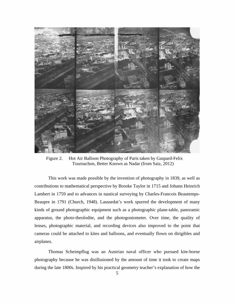
5

Figure 2. Hot Air Balloon Photography of Paris taken by Gaspard-Felix Tournachon, Better Known as Nadar (from Saiz, 2012)

This work was made possible by the invention of photography in 1839, as well as

contributions to mathematical perspective by Brooke Taylor in 1715 and Johann Heinrich

Lambert in 1759 and to advances in nautical surveying by Charles-Francois Beautemps-

Beaupre in 1791 (Church, 1948). Laussedat’s work spurred the development of many

kinds of ground photographic equipment such as a photographic plane-table, panoramic

apparatus, the photo-theolodite, and the photogoniometer. Over time, the quality of

lenses, photographic material, and recording devices also improved to the point that

cameras could be attached to kites and balloons, and eventually flown on dirigibles and

airplanes.

Thomas Scheimpflug was an Austrian naval officer who pursued kite-borne

photography because he was disillusioned by the amount of time it took to create maps

during the late 1800s. Inspired by his practical geometry teacher’s explanation of how the

6

new science of photogrammetry was much faster than manual point-to-point image

correlation young Thomas set forth to develop the “photo karte,” a distortion-free

photograph that could be used to make highly accurate maps (Erdkamp, 2011). Utilizing

ideas from a 1901 British patent submitted by Parisian engineer, Jules Carpentier, he was

able to submit his own patent in 1904 describing an apparatus to alter or (un)distort

photographs (Merklinger, 1996). In this work, he described what would later become

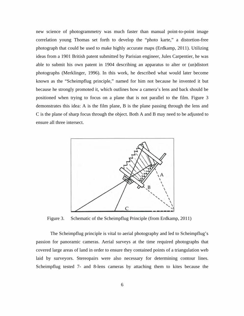
known as the “Scheimpflug principle,” named for him not because he invented it but

because he strongly promoted it, which outlines how a camera’s lens and back should be

positioned when trying to focus on a plane that is not parallel to the film. Figure 3

demonstrates this idea: A is the film plane, B is the plane passing through the lens and

C is the plane of sharp focus through the object. Both A and B may need to be adjusted to

ensure all three intersect.

Figure 3. Schematic of the Scheimpflug Principle (from Erdkamp, 2011)

The Scheimpflug principle is vital to aerial photography and led to Scheimpflug’s

passion for panoramic cameras. Aerial surveys at the time required photographs that

covered large areas of land in order to ensure they contained points of a triangulation web

laid by surveyors. Stereopairs were also necessary for determining contour lines.

Scheimpflug tested 7- and 8-lens cameras by attaching them to kites because the

7

multitude of angles provided more than 100-degree views of the ground. His most

popular camera configurations are shown in Figure 4.

Figure 4. Scheimpflug’s Camera Configurations (from Erdkamp, 2011)

For the actual map-making one more piece of equipment was needed: the “photo

perspektograph” camera. This device, seen in Figure 5, processed aerial photographs to

remove distortion by compensating for the decrease in scale proportional to the distance

from the camera. This distorting enlarger corrected object proportions and positioned

8

them where they ought to be on a conventional map (Erdkamp, 2011). Finally, maps

could be made directly from corrected photographs.

Figure 5. Scheimpflug’s Photo Perspektograph Model II (from Erdkamp, 2011)

Captain Cesare Tardivo was as dedicated to aerial imagery and surveying as

Thomas Scheimpflug. After many years of working with hot air balloons as a member of

the Photographic Section of the Italian Specialist Brigade, Tardivo was able to present

surveys, such as the one seen in Figure 6, to the International Conference of Photography

(Guerra & Pilot, 2000). The success of this topographic survey of Ostia (Antica), the

location of ancient Rome’s harbor city, finished in 1911, helped convince military and

civilian groups of the utility of this new discipline.

9

Figure 6. Topographic Survey of Ostia from a Hot Air Balloon (from Shepherd, 2006)

As support and interest grew, Tardivo wrote a book on the subject. His “Manual

of Photography, Telephotography, and Topography from Balloon” explains many aspects

of surveying, from appropriate weather conditions and the dimensions required for a

balloon to carry certain instruments to the need of having a tailor on the collection team

in case of repairs (1911). As inferred from in Figure 7, large numbers of images were

required in order to cover any sizable area because only the centers of each photograph

were geometrically correct enough for use in maps, and successive images were rarely

aligned. With the invention of the airplane in 1903 this changed drastically because

images could be collected quickly and efficiently, following pre-planned flight paths in

controlled directions.

10

Figure 7. Mosaic of Images Taken of Ostia For Use in the Topographic Survey by Hot Air Balloon (from Shepherd, 2006)

In the United States, terrestrial photographs were first used for topographic

mapping in 1904 when a panoramic camera was taken to Alaska by the United States

Geological Survey (USGS) (Church, 1948). Topographic maps depict terrain in three

dimensions with the topographic relief usually represented by contour lines. James

Bagley documented and later published much of what he learned firsthand about

terrestrial surveying and applying photogrammetry to aerial surveys (1917). He and

another member of the USGS team to Alaska, F. H. Moffitt, were inspired to build a

three-lens camera, as seen in Figure 8, based on the cameras of Thomas Scheimpflug.

11

Figure 8. Three-Lens Camera Used by USGS Team in Alaska, with One Vertical and Two Obliques (from “Early Techniques,” 2000)

The T-1, their tri-lens camera built in 1916, had “one lens pointing vertically

downward and two lenses inclined 35 degrees from the vertical” (Church, 1948). This

setup allowed crews to collect photographs of a flight path from three separate angles on

a single pass. This three-lens method created less distortion than the wide angle lenses

that were popular at the time. As World War I progressed, Bagley was sent to France to

continue work on the tri-lens camera and after the war he stayed on with the Army at

McCook Field. Advances made over the next 25 years proved invaluable to the United

States’ World War II military forces. Aerial photographs were used to prepare

aeronautical charts of inaccessible areas, to mark enemy positions and movements on

maps, and to plan invasions. More domestic uses of aerial photography and

photogrammetric products include investigations by oil, lumber, and power companies,

highway and railroad commissions, inventorying, and forestry.

12

1. Mechanics behind Photogrammetry

Stereoscopic vision allows an observer to see the height and depth of a

photograph in addition to lengths and widths. The phenomenon of depth perception is

possible due to the physical distance between the human eyes as this provides the brain

with slightly different viewing angles of the same scene. An equivalent setup can be

accomplished artificially by taking photographs of the same object or scene from

different angles and viewing them side by side with a scanning stereoscope, as seen in

Figure 9.

Figure 9. Scanning Stereoscope (from “Old Delft,” 2009)

A stereoscope allows an observer to look at the two overlapping photographs of a

stereopair simultaneously but with each eye looking at one image instead of both eyes

looking at the same image. To work correctly the photographs are taken in the same plane

and lined up parallel to the ocular base of the instrument. For vertical aerial photographs

the line of flight of the aircraft should be used to align the photographs on the instrument.

When prepared correctly, the result is a miniature model seen in relief, called a

13

stereoscopic model or stereogram. Another technique for obtaining stereoscopic models

includes printing two overlapping photographs in complementary colors on the same

sheet. Special glasses are worn, with each lens being tinted the same color as one of the

images, so that the observer sees one photograph with each eye. This creates a miniature

relief model in black and white (Church, 1948).

For measuring distances in the models supplementary tools are needed. A

measuring stereoscope includes a “floating mark” in each eye-piece to help define the

line of sight and measure parallaxes. A stereocomparator additionally has a “system for

reading the rectangular coordinates upon its photograph” (Church, 1948). In order to

draw planimetric and topographic maps a multiplex projector is required. This instrument

utilizes a collection of projectors to display adjacent photographs onto a plotting table,

called a platen (Church, 1948). Two projectors are used at a time, one with a red lens and

the other with a blue-green lens, and when their rays intersect the observer moves the

platen around the model to mark different elevations on the map (Church, 1948).

2. Computer Photogrammetry and MVS

It had been hypothesized since the 1960s that computers could be used to analyze

imagery. In 1969, Azriel Rosenfeld suggested methods for classifying entire images by

the relationships among objects within them (Rosenfeld, 1969). Two years later, Lynn

Quam reported on digital techniques for detecting change between images including

those taken from different viewing angles (1971). As seen in Figure 10, simple change

detection was completed by differencing two images, with areas of high dissimilarity

indicating a change between the two. Papers such as these laid a foundation for future

computer vision work and digital photogrammetry.

14

Figure 10. Quam Differenced Two Images from the 1969 Mariner Mission to Mars as a Form of Change Detection (from Quam, 1971, p. 77)

According to Dr. Joseph Mundy, the goal of digital photogrammetry is to “find

the set of camera parameters, image feature positions and ground control point positions”

that minimizes total error (1993). In manual photogrammetry exact camera parameters

and positions are known because photogrammetrists strictly collect such information for

mapmaking. Although time-consuming, it is fairly easy to match features in stereopairs

because the two photographs are taken from similar angles.

Some computer software, such as BAE Systems’ SoftCopy Exploitation Toolkit,

(SOCET) follows strict photogrammetric rules. SOCET originated from fully digital

analytical plotters, called photogrammetric workstations, created by photogrammetrist

Uuno Vilho Helava in the 1970s (Walker, 2007). While these plotters have become more

automatic over the years they still require a good deal of manual input. Large amounts of

camera information are required to register images because SOCET relies on “faithful,

mathematical sensor modeling” and image metadata to orient and triangulate imagery

15

(Walker, 2007). Possible SOCET inputs include camera model, interior and exterior

orientation, calibration information, and GPS location, as well as tie points or ground

controls points (GCPs). Products include 2-dimensional (2D) feature mapping around

buildings, 3D point clouds either regularly gridded or in a Triangular Irregular Network

(TIN), DEMs, DSMs, ortho-images, and mosaics.

In 2013, an initial comparison revealed that stereo point clouds created with

SOCET using either aerial or satellite imagery accurately portrayed object locations but

vegetation and building edges were less defined than LiDAR point clouds (Basgall,

2013). The difficulty with vertical walls around buildings was due to the method of point

cloud creation. SOCET’s stereo point cloud generator first created a DEM, which

identified matching points between the images but continued by interpolating to create a

0.15m grid. This means that where cars, trees, or buildings were in close proximity the

surface morphed them together in the DEM and the output point cloud. The result is not

surprising because most photogrammetric outputs are actually 2.5-dimensional (2.5D)

meaning they do not allow more than one point at any x,y location even with distinct z

values. This makes representing truly vertical walls impossible, leaving them as

unknowns in most models. Matching vegetation between images is also challenging

because separate leaves and branches may move between collections or may be smaller

than the image resolution. Even facing these difficulties Basgall’s comparison revealed

the SOCET output could still be used for change detection of sizable events (2013).

New software with roots in the computer vision community is trying to make

image registration fully automatic. By teaching computers how to match features

between images the human component is removed. A survey by professors at the

University of Washington concluded there are four main categories of multiview stereo

(MVS) algorithms (Seitz, 2006). The first of these compute a cost function to determine

which surfaces to extract from a 3D volume. Seitz and Dyer proposed a method for

coloring voxels by finding locations that stay constant throughout a set of images (1999).

A second class includes space carving techniques such as those based on voxels, level

sets, or surface meshes that progressively remove parts of a volume according to the

imagery (Seitz, 2006). One of these methods, described by Eisert, Steinbach, and Girod,

16

uses two steps to first, assign color hypotheses to every voxel according to the

incorporated images and second, either assign a consistent color or remove the voxel

(1999). Algorithms in the third class compute depth maps for input images and merge

them together to create coherent surfaces (Gargallo & Sturm, 2005). The last class

includes methods which extract and match features between images before fitting a

surface to the registered points. Morris and Kanade suggested starting with a rough

triangulation of a surface and refining it to better represent the objects found within the

input images (2000).

Due to the vast number of pixels found in a single image and the amount of time

it takes to compare all of them, older algorithms were taught to identify a handful of

unique features and compare those to the unique features found in other images. Now that

computer hardware has progressed, lifting previous time constraints, dense pixel-wise

matching algorithms are available that can search every pixel or window of pixels for a

match (Hirschmuller, 2005). The large numbers of matches found in this way allow for

the creation of very detailed 3D models. Heiko Hirshmuller’s semi-global matching

(SGM) algorithm maintains sharper object boundaries than local methods and

implements mutual information (MI) based matching instead of intensity based matching

because it “is robust against many complex intensity transformations and even

reflections” (2005). SGM’s pathwise aggregation uses cost information from eight

directions to minimize disparity, with its major attraction being that its runtime is linear

to the number of pixels and disparities (Hirshmuller, 2011).

Developments in the computer vision community over the last 10 years have also

led to the creation of algorithms that can determine camera orientation automatically.

Software such as Bundler, Microsoft Photosynth, Agisoft PhotoScan and PhotoModeler

solve for camera parameters and generate 3D point clouds of either objects or scenes

(Harwin, 2012). Some can reconstruct objects and buildings from unorganized collections

of photographs taken from different cameras at multiple distances, viewing angles, and

levels of illumination (Agarwal, 2011). Matching features in such dissimilar images

requires identifying interest points within each photograph, with the more rigorous

algorithms finding affine-, in-plane rotation-, translation-, and illumination-invariant

17

features (Van Gool, 2002). The scale invariant feature transform (SIFT) operator has

proven especially robust and has grown in use since 2004 (Lindeberg, 2012).

Structure from motion (SfM) is another technology that utilizes multiview

techniques. It falls between photogrammetry and MVS by using overlapping photographs

taken by a single camera around an object. The motion of the camera between semi-

stereopairs is used to determine position and orientation so the correct geometry can be

applied to build 3D models. See Figure 11 for an illustration of the relationships between

the three techniques mentioned.

Figure 11. Block Diagram Illustrating Relationships between Image-to-Model Techniques

3. How It Works

Triangulation is the basic mathematical concept behind photogrammetry. Stereo

vision exploits the slightly different views between two photographs to derive depth and

create 3D models. As seen in Figure 12, it is necessary to know the two camera locations

(C1 and C2) in order to correctly locate the objects (P and Q) in 3D space according to

their images (P’1, P’2, Q’1, and Q’2). Accurate image correspondences are required for

3D reconstruction so coordinates can be derived from intersecting optical rays (Faugeras

& Keriven, 2002). By finding the intersection of the lines extending from each camera

through its respective image, the depth of each object can be determined.

18

Figure 12. Deriving Depths of Points P and Q using Two Images (from “Image-based Measurements,” 2008)

If the camera’s position and aiming angle are unknown, resection is required to

determine the missing information. Resection uses a given image to determine three

position coordinates and three angles in order to correctly derive the location of the

camera and the angle it was pointing at the time the photograph was taken. Resection, if

done manually, is a long tedious process, which is why the automatic computer vision

approach is highly desirable. Cameras must also be calibrated before use so that detected

errors can be removed before imagery is processed. Altogether these techniques

(triangulation, resection, calibration) are referred to as the bundle adjustment. In some

computer vision algorithms triangulation and resection are computed at the same time,

minimizing errors in each until an optimal solution is found.

Once feature coordinates are determined, points are created in 3D space.

Photogrammetric point clouds are limited to the area of overlap between the two included

images and can only contain one height coordinate for each latitude and longitude,

similar to LiDAR point clouds. MVS point clouds are not quite as limited, revealing

walls and other vertical structures provided they were visible in multiple images and

correctly matched.

19

B. LIDAR BACKGROUND

While most people are familiar with radar and its ability to determine the location

of objects by using radio waves, light detection and ranging (LiDAR) has gained

popularity within the last 30 years. LiDAR is a technology that utilizes many radar

principles, but applies them to shorter wavelengths: in the visible to infrared range.

Surveyors used the first terrestrial laser instruments to replace tungsten and

mercury vapor lamps in the 1970s. Newly invented lasers allowed a small team to

measure long distances and apply trilateration techniques in order to create topographic

maps quickly and efficiently (Shan & Toth, 2009). Current electronic total stations

(ETSs) measure angles and distances from their location to that of their corresponding

prism reflector using modulated infrared signals. Figure 13 shows how ETSs can

determine vertical height measurements that are out of reach of ground-based prisms.

Figure 13. Electronic Total Stations Measure Heights of Unreachable Objects Via Remote Elevation Measurement (from “Total Station,” n.d.)

20

By timing how long it takes the infrared signal to travel to and from the prism,

very accurate distances can be determined. This idea, when carried out in a scanning

mode, allows one unit to measure distances to multiple objects, returning large numbers

of points that can be converted into 3D space and used to build 3D models. Terrestrial

LiDAR has been found useful in a multitude of applications such as “bridge and dam

monitoring, architectural restoration, facilities inventory, crime and accident scene

analysis, landslide and erosion mapping, and manufacturing” (Schuckman, 2014).

LiDAR has also been adapted to collect from airborne platforms. When carried on

the underside of an airplane or unmanned aerial vehicle (UAV) large swaths of land can

be covered in a few hours. Airborne sensors usually operate in a whiskbroom mode,

sweeping a laser in a “sawtooth” pattern of points, back and forth across the flight path.

This mode takes advantage of the forward motion of the aircraft to cover the ground

below (Diaz, 2011). The speed of the aircraft and the pulse rate of the sensor determine

the resolution, or point density, of the point cloud that can be created. Airborne systems

are able to concentrate on moderately sized areas such as cities, coastlines, and national

parks. Multiple flight lines are collected, usually in parallel, with enough overlap so each

strip can be stitched to adjacent ones and a continuous surface model can be created.

1. Physics of LiDAR Systems

Modern LiDAR units consist of three integral components, seen in Figure 14, to

ensure accuracy and usability of the collected data. The laser rangefinder is arguably the

most important apparatus, as it actively emits and then collects laser energy like the

terrestial ETSs, but for airborne systems the Global Positioning System (GPS) and the

inertial measurements unit (IMU) are required if the collected data is to be geolocated

and correctly fused.

21

Figure 14. Main Components of Airborne LiDAR (from Diaz, 2011)

The main laser unit employs a laser which emits pulses of photons. When these

pulses travel to the ground, reflect off objects and the earth’s surface, and return to the

aircraft the photodetector collects and records their intensity level and time of return.

Most systems use the time of flight (TOF) method to determine the range of the objects

illuminated by the laser. The TOF method determines the distance between the aircraft

and the illuminated object, providing the height information for post-processed points in

the 3D model. Due to atmospheric effects, mechanical issues, and human error it is

impossible for an aircraft to stay perfectly straight and level during a survey so an IMU is

also required. IMUs take these factors into account and precisely track the attitude of the

aircraft, recording changes in the roll, pitch, and yaw at all times during a collection so

that these measurements can be processed with the data.

22

GPS systems provide position and velocity information so that points within the

data set can be referenced to real points on the surface of the earth. Due to factors such as

the wavelength of light produced by the laser source, the pulse repetition frequency

(PRF), and the speed of the aircraft, the entire surface of the ground will not be mapped.

Instead, points will be collected at intervals along the laser’s path. The point density,

usually measured per square meter, indicates the resolution of objects that can be seen in

a particular scan.

Once all points are collected, flight paths are stitched together and software is

used to visualize the 3D point cloud. The GPS provides the x and y coordinates, latitude

and longitude, while the determined range indicates the z, or altitude coordinate. Certain

software can now identify points within a point cloud according to height and separate

them into categories such as ground, buildings, and trees. If color imagery is collected of

the same area on the ground, software can overlay this data onto the point cloud to

produce true-color 3D scenes. The best results occur when the LiDAR scan and imagery

are taken simultaneously so that objects prone to movement, such as cars, people, and

water, appear in the exact same location in both datasets.

23

III. DATA AND SOFTWARE

A. LIDAR AND IMAGERY OF NPS

LiDAR data were collected in October of 2012 by Watershed Sciences, Inc.

(WSI). It utilized an Optech Orion C200 laser system flown on a Bell 206 LongRanger

helicopter. A good portion of the Monterey Peninsula was collected; Figure 15 shows the

extent of the area around the Naval Postgraduate School (NPS) to be studied here. As the

LiDAR data were saved in tiles less than 200 Megabytes, 12 such tiles were required to

represent the entire NPS campus.

Figure 15. LiDAR Dataset of the NPS Campus East of the Monterey Peninsula (map from Google Maps, n.d.)

24

Even flying at 450m altitude the LiDAR point cloud was very dense at

approximately 30 points/m2, allowing for sub-meter objects to be identified. The point

cloud seen below includes RGB coloring from photographs taken of the same area. This

extra encoding aids in the identification of different surfaces. Figure 16 demonstrates

how the vertical surfaces of buildings, such as the front façade of Hermann Hall, are

missing due to the vertical nature of LiDAR collection. However, details such as roof

shape, tree leaves, cars in the parking lot, and even the flagpole are present. Compare the

structures shown in the LiDAR dataset to a photograph taken of Hermann Hall and the

surrounding buildings.

Figure 16. LiDAR Dataset Compared to a Photograph of Hermann Hall (from “NPS Statistics,” 2014)

25

B. AIRBORNE DATA

Optical imagery was obtained in both October 2013 and May 2014 using a

Hasselblad H4D-50 50 megapixel camera. This imagery was likely taken from a small

airplane similar to a Partenavia SPA P68C from an altitude of 433m which produced 5cm

pixel resolution (University of Texas, 2013). In both the October and May collects six of

the images contained Glasgow Hall. Figure 17 illustrates the quality of the 2013

Hasselblad imagery used for this study.

Figure 17. Close-up Near-nadir View of Glasgow Hall Aerial Imagery

26

Table 1 shows the similarity between the May and October collects. The two

sequences were photographed from near-identical flight paths so the pairs are very

similar. The top row exhibits the October 2013 images, taken during Monterey’s sunny

Indian summer, while the bottom row was taken in May 2014 on a cloudy day, useful

because of the lack of shadows. They have been arranged so that the building’s south side

can be viewed in a west-to-east direction in the first three images, followed by three near-

nadir views.

Table 1. Comparison of October 2013 and May 2014 Hasselblad Imagery (Oriented Roughly North-South)

Aerial imagery was also collected by Watershed Sciences, Inc (WSI) in October

2012. This collection was flown at 450m yielding a pixel resolution of 10-15cm with an

UltraCam Eagle camera produced by Microsoft. Again, six of the images contain

Glasgow Hall, and due to very oblique angles in three of the images the rear of the

building is visible. In Table 2, the first three images show the south side of Glasgow on a

west-to-east flight path and the last three images similarly show the north side.

Table 2. UltraCam Eagle Imagery of Glasgow Hall

27

C. SATELLITE DATA

A small collection of satellite imagery covering the Monterey, CA area over the

years 2000 to 2011 was accessed, providing seven usable images of NPS. Table 3

exhibits each image and provides the panchromatic resolution given on the Digital Globe

website for each of the mentioned satellites.

Table 3. Satellite Imagery Thumbnails, Date of Collection, Run Number, and Details (after Digital Globe, 2013)

28

The IKONOS satellite is the oldest one of the group, having been in orbit since

1999. Following the launch of IKONOS were those of Quickbird I in 2001, Worldview-1

in 2007, and GeoEye-1 (previously Orbview 5) in 2008 (Digital Globe, 2013).

D. SOFTWARE

The IMAGINE Photogrammetry software application, formerly Leica

Photogrammetry Suite, extracts information from stereopairs to create 3D models. In the

works since 2003, it now contains three methods for producing terrain models. The

automatic terrain extraction (ATE) process creates medium density DTMs rapidly and

requires little manual editing. The enhanced ATE (eATE) process generates higher

resolution models using stereopairs and can also take advantage of parallel processing to

decrease runtime. The 2014 release of IMAGINE Photogrammetry unveiled a SGM

algorithm that can create models with point spacing to rival that of LiDAR. SGM is

currently only applicable to aerial imagery but Intergraph is looking to update the

algorithm for its 2015 release. For this thesis the eATE module was applied to both aerial

imagery, in TIF, and satellite imagery, in NTF.

For MVS purposes, Agisoft Photoscan Professional, from here on referred to as

Agisoft, offered itself as a suitable software package. Agisoft allows any user to upload a

variety of photos and generate 3D models. The software is sensor ambiguous as it

completes a bundle adjustment for each image without supplementary information,

determining camera angle and location before building 3D models automatically. While

created to work with aerial imagery, Agisoft was able to ingest satellite photos once

they’d been converted to TIFF. The product website also indicates it can accept inputs of

JPEG, PNG, and BMP.

Quick Terrain Modeler (QTM) and CloudCompare (CC) are visualization

packages designed to display 3D point clouds. They both have the capacity to express

multiple models simultaneously making side-by-side comparison possible.

29

IV. PROCESSING, RESULTS, AND ANALYSIS

A. AERIAL IMAGERY MULTIVIEW STEREO

Having access to three aerial imagery datasets allowed for a number of

combinations to be tested. The Agisoft website and those of similar software packages

lead a user to believe that the more images included in the process the more complete the

model turns out. It was found this was not necessarily the case, as explained in the three

trials below.

The two Hasselblad datasets were collected using similar flight paths so the

images provided only slightly different views of Glasgow Hall, while the WSI dataset

included very oblique angles and provided much better views of the sides of the building.

Trial #1 used equal numbers of images from each dataset, working from one to six so that

the first trial was composed of three images and the last trial contained all 18. In Trial #2

the best model created in Trial #1 was compared to dense models created with the six

images in each separate dataset. Finally, Trial #3 dissected the winning model from Trial

#2 to see if all six images were really necessary or whether a model created using three,

four, or five photographs was sufficient, or even superior in completeness.

1. Trial #1

Images in this trial were added in such a way as to provide the most new

information in the first three runs before adding the repeat images from the Hasselblad

datasets. Because the WSI imagery covered a much larger area, each image had to be

subset within Agisoft to focus on the Glasgow Hall area. Subsets included Glasgow Hall,

the Dudley Knox Library, and surrounding parking lots in order to cover the same subject

matter as the Hasselblad imagery, as seen in Figure 18. This was the extent of pre-

processing required by the Agisoft software.

30

Figure 18. WSI Image Subset to Glasgow Hall and Dudley Knox Library

After adding the preferred images (Workflow > Add Photos… > select from

library) a sparse point cloud preceded any advanced models. The sparse cloud was

created by aligning the photos (Workflow > Align Photos…), which is when Agisoft

performs a bundle adjustment on each image to determine its location and pointing angle.

The sparse point cloud is only a rough sketch, as seen in Figure 19. Each blue rectangle

represents a camera’s suggested position and the black line stemming toward the image

name provides the suggested angle. In the lower left corner of the main window, the

sparse point cloud is seen as white and gray points.

31

Figure 19. Three Aligned Photos (One Off-screen) and Sparse Point Cloud

After the sparse point cloud laid the groundwork, the now-registered images

were re-evaluated for matching features and a dense point cloud was created. As seen in

Figure 20, dense clouds reveal structures and textures, especially when color imagery is

available. The incompleteness of this dense point cloud was due to the lack of

information, as only three images were run in this trial.

32

Figure 20. Sparse and Dense Aerial Point Clouds in Agisoft

In Table 4, the progression of dense point clouds appears to reveal improvements

from the first to the fourth runs. While the fifth and sixth runs begin to display pieces of

Glasgow’s southern wall they also appear fuzzy and speckled. The shape of Glasgow’s

roof is hardly discernable in the last run, indicating that adding more images degraded the

model. For this trial Run #4 claims the title for best model.

33

Table 4. Dense Points Clouds for Trials Utilizing All Three Datasets

34

2. Trial #2

The goal of Trial #2 was to determine whether a single dataset could compete

with the results of the combined dataset. Using Run #4 as the winner of Trial #1, the

steps already mentioned were repeated for each of the image collections separately. Table

5 shows the WSI model a clear winner, as it contains the fewest holes, the most

vegetation, and even walls of buildings.

Table 5. Models of Each Six-Image Collection Compared to Winning Combined Model, Using Aerial Imagery

35

3. Trial #3

For the final trial, the winning WSI model from Trial #2 was further evaluated.

The first run started with three WSI images, chosen so that the largest differences in

camera angle might provide the most information, with the last run containing all six

images. Table 6 demonstrates changes between the models.

Table 6. Comparison of WSI Models

36

The winning model is not the expected run containing all six images. Comparing

Run #3 and Run #4, small differences indicate a greater level of completeness in the

model of only five images. Starting with the buildings it should be noted that the walls of

Glasgow’s highest protrusion, a white square-shaped room, are more complete in Run #3.

Similarly, Glasgow’s southernmost wall has fewer and smaller holes. This trend extends

to the walls of the library and other nearby buildings. Due to the small number of images

incorporated into these models the results seen above are surprising.

To further investigate the puzzling findings above another run was completed,

switching the fifth and sixth images. In Run #3 of the last trial the fifth image was taken

from a north-facing position while the sixth image was taken from a south-facing

position. As seen in Table 7, by focusing on only the south walls of the buildings in Trial

#3 half of the information was missed. In Table 7 it becomes clear the fifth images

provided the information allowing Agisoft to model the building walls: the original five

covering the southern walls and the new five covering the northern walls. After

considering all views of Glasgow, the run containing all six images reclaims the title of

best model, as it represents building walls on all sides, albeit incompletely.

This trial revealed that the order in which the images were added to the model

changed the points registered with each iteration. If all images are eventually going to be

included this does not affect the final outcome but for situations in which the number of

images is limited care should be taken to include those containing the most unique

information.

37

Table 7. WSI Models of Five and Six Images

. WSI Model with All 6 Images: South Side

38

B. SATELLITE IMAGERY MULTIVIEW STEREO

As Agisoft could not ingest the satellite images provided in National Imagery

Transmission Format (NITF) they were converted to Tagged Image File Format (TIF).

Then each image histogram was stretched to cover the full bit range to create the greatest

contrast between shades of gray. AgiSoft was run with each set of images; first by

aligning them and creating a sparse point cloud, and then creating a dense point cloud

after the model passed initial inspection. Table 8 shows the progression of images run

through the software. The first three include one of each resolution, followed by the

IKONOS images at the lowest resolution of 82 cm, and finally by the higher resolution

images at 46 cm.

Image # Run # Year Month Day Satellite Panchromatic Resolution 1 1 2000 Nov 28 IKONOS 82 cm 32 in 3 1 2002 Sep 21 Quickbird II 61 cm 24 in 6 1 2009 Oct 28 Worldview 1 46 cm 18 in 4 2 2002 Oct 29 IKONOS 82 cm 32 in 2 3 2000 Nov 28 IKONOS 82 cm 32 in 5 4 2008 Dec 26 Worldview 1 46 cm 18 in 7 5 2011 Jan 19 GeoEye 1 46 cm 18 in

Table 8. Order Satellite Images were added to Agisoft Photoscan Pro

After completing each run the dense point cloud was exported in .las format and

viewed in QTModeler software for comparison. As seen in Table 9, with each image

addition more of the Monterey Peninsula became visible. By returning to Table 3 the

reader can see that while the three original satellite images cover much of the same area

only a thin strip of the peninsula was correctly registered. Another oddity is found in the

run of five images where the northeastern tip of the peninsula is missing when it was

clearly present in the run before, a run containing four of the same images.

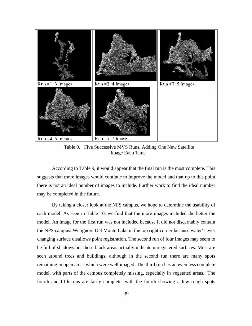
39

Table 9. Five Successive MVS Runs, Adding One New Satellite Image Each Time

According to Table 9, it would appear that the final run is the most complete. This

suggests that more images would continue to improve the model and that up to this point

there is not an ideal number of images to include. Further work to find the ideal number

may be completed in the future.

By taking a closer look at the NPS campus, we hope to determine the usability of

each model. As seen in Table 10, we find that the more images included the better the

model. An image for the first run was not included because it did not discernably contain

the NPS campus. We ignore Del Monte Lake in the top right corner because water’s ever

changing surface disallows point registration. The second run of four images may seem to

be full of shadows but these black areas actually indicate unregistered surfaces. Most are

seen around trees and buildings, although in the second run there are many spots

remaining in open areas which were well imaged. The third run has an even less complete

model, with parts of the campus completely missing, especially in vegetated areas. The

fourth and fifth runs are fairly complete, with the fourth showing a few rough spots

40

around forested areas and the fifth missing part of a baseball diamond and parking lot, as

well as some of the academic buildings on the west end of campus.

Table 10. Satellite MVS Close-up of NPS

If we were only interested in the nadir view of each model we could simply

compare each one to a map of the area. When considering 3D models we must also

evaluate the altitude or elevation component, the third element of xyz models. The

second run appears to have points on at least four different planes, while the third, fourth,

and fifth runs appear to contain five, four, and two planes, respectively. It appears the

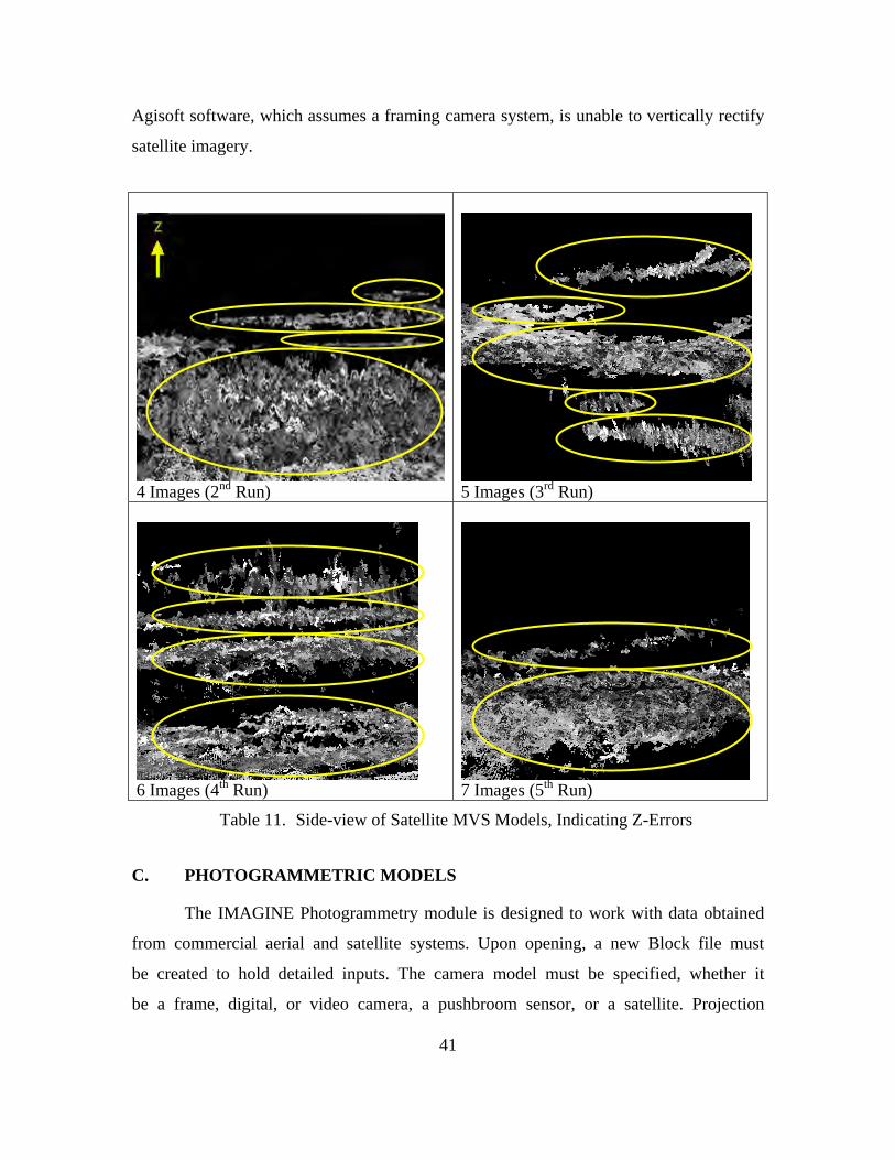
41

Agisoft software, which assumes a framing camera system, is unable to vertically rectify

satellite imagery.

4 Images (2nd Run)

5 Images (3rd Run)

6 Images (4th Run)

7 Images (5th Run)

Table 11. Side-view of Satellite MVS Models, Indicating Z-Errors

C. PHOTOGRAMMETRIC MODELS

The IMAGINE Photogrammetry module is designed to work with data obtained

from commercial aerial and satellite systems. Upon opening, a new Block file must

be created to hold detailed inputs. The camera model must be specified, whether it

be a frame, digital, or video camera, a pushbroom sensor, or a satellite. Projection

42

information, camera values, and tie points are also required before any type of processing

can occur.

1. Aerial Imagery

As the UltraCam Eagle used to collect the WSI imagery is a digital camera this

option was chosen. Next, a reference coordinate system was needed; in this case the

defaults of a Geographic projection and WGS 84 Datum were left untouched. There are

many options for projections and if this information was missing these selections could

be left as “unknown.” The next piece of required information was the average flying

height, in this case 450m.

Once the preliminaries were entered, images could finally be added (right click on

“Images” > Add > select from library). More information then had to be included to

categorize the interior and exterior orientation of the camera. Specifically the pixel size,

perspective center, and rotation angles were needed, which were accessed by right-

clicking one of the red boxes under the intended heading.

The next step could have been accomplished in a few different ways. IMAGINE

Photogrammetry was programmed to accept both GCPs and/or tie points so as long as

enough of one or both were created triangulation could be completed. Clicking on the

crosshairs symbol opened the point measurement window. Here both images were

viewed simultaneously so that identical points could be created to tie them together.

When GPS information was available the point was marked as “Control” in the “Usage”

column and the x/y/z values were entered, otherwise it was labeled as “Tie.” Once an

acceptable number of points were marked, “Automatic Tie Generation” (the symbol

looks like a plus sign inside a circle of arrows) was run in order to lessen the workload,

although all created tie points had to be checked for accuracy before use. As seen in

Figure 21, each point had to be as exact as possible, with zoom windows available to

mark them to pixel accuracy.

43

Figure 21. IMAGINE Photogrammetry’s Point Measurement Window

The last step in this window was to “Perform Triangulation” (the blue triangle

symbol). This caused the image outlines in the main window to overlap according to their

newly determined positions. The images needed to overlap more than 30% for IMAGINE

to process them. Figure 22 demonstrates a correctly aligned and marked pair, with GCPs

represented as red triangles and tie points shown as red squares.

44

Figure 22. GCPs and Tie Points in IMAGINE Photogrammetry

Finally, the actual photogrammetry could be completed. The blue “Z” symbol

seen at the top of Figure 22 is the “DTM Extraction” tool, from which “eATE” was

selected as the preferred method. In the eATE Manager window the last two steps were to

click “Generate Processing Elements” (from the Process tab), which highlighted the

overlapping area between the images, followed by “Batch Run eATE…” (also under the

Process tab) and clicking the “Run Now” button. Depending on the size of the images,

final processing took from 30 minutes to hours to complete. The result obtained by

entering two of the WSI images can be seen in Figure 23. In spite of doing a fair job of

outlining most of the major features, this model is quite lean. Points along color

boundaries appear to have been the easiest to associate, indicating the algorithm searches

for unique color features to match between the two images. The top portion of Figure 23,

a horizontal view of the model, reveals that most of the points represent surfaces at a

believable range of elevations, a good portion of them existing on the ground and several

others at the levels of trees and building roofs (green and white, respectively).

45

Figure 23. Photogrammetry Point Cloud of Glasgow Hall, Aerial Imagery

2. Satellite Imagery

Setting up the Photogrammetry module with satellite imagery was much faster

than with aerial imagery because the only information that had to be manually entered

was the camera/satellite type and the correct projection and datum. Because all of the

46

auxiliary information for satellite images is included within rational polynomial

coefficient (RPC) files or provided NTFs, all that was necessary was to select the

preferred photogrammetry method and run it.

In keeping with the results found in the aerial imagery MVS section, it was

decided to use two images from the same satellite for this experiment. This limited the

choice to three IKONOS images or two Worldview images, the latter of which did not

provide enough overlap. Upon examination, the 2000 November 28 #1 image and the

2002 October 29 image were chosen; they can be seen in Table 3. IKONOS images are

provided as NTFs so after specifying the sensor type and Universal Transverse Mercator

(UTM) projection of Zone 10, with a World Geodetic System 1984 (WGS 84) datum the

manual work was concluded by selecting and running the eATE method.

Figure 24 reveals the panchromatic photogrammetric model created of the

Monterey Peninsula. Similar to the aerial result, this model appears to have registered

points lying on color boundaries the best, such as roads and buildings. The top view of

the figure reveals the elevation changes detected by the model, which generally match the

elevations indicated by the red line running through the topographic map to the left.

47

Figure 24. Stereo Photogrammetry Point Cloud of Monterey, CA; Horizontal View of the Southern Edge (Top), Topographic Map (Left, after

“Digital Wisdom,” 2014), Nadir View (Bottom)

D. COMPARISON WITH LIDAR

Turning to the CloudCompare software, the LiDAR, IMAGINE, and Agisoft

models were opened simultaneously and aligned. Using the LiDAR point cloud as ground

truth for the location of objects and buildings, the photogrammetric and MVS datasets

were translated and rotated to match. Tables 12 through 16 demonstrate the differences

between the three point clouds from different points of view. The first window of each

table demonstrates how difficult it was to determine differences between the color

models. To solve this problem, the points of the photogrammetric point cloud were

changed to purple and those of the MVS point cloud were rendered in yellow with the

LiDAR points in white or left as true color.

48

1. Aerial

The overall meagerness of the photogrammetry point cloud made finding matches

between models problematic because the IMAGINE software identified edges of objects

but failed to render any kind of homogenous areas such as concrete roads or parking lots,

dirt, grass, or building roofs. In Table 12, the main takeaway is that none of the roof

points extend into the “shadow” of the wall on the south or west sides of Glasgow Hall.

In Table 13, it becomes apparent that the photogrammetry model contains the Glasgow

building but it is shifted to the northeast. This can be explained by a characteristic of

aerial photography known as relief displacement. This geometric distortion is due to

elevation changes and is particularly disturbing in urban areas with tall buildings.

Because stereo photogrammetry only makes use of two images it is not surprising this

distortion appears in the 3D model.

There is slightly more to be said of the MVS model, in that the entire shape of the

building hugs that of the LiDAR model, to include segments of wall on all sides. There

are a few dissimilarities seen in the concavities of the building where the MVS model has

rounded some of the surfaces instead of providing straight edges, but at least the walls are

present.

49

Table 12. Comparing Imagery Results to LiDAR Ground Truth (View of Glasgow Hall from the Southwest)

50

Table 13. Comparing Imagery Results to LiDAR Ground Truth (View of Glasgow Hall from the Northeast)

Transects of the images seen in Figure 25 demonstrate how closely

photogrammetric and MVS models follow the surface of the LiDAR data. The points

delineating the ground closely overlap with little to no deviation between the three

models. Where vegetation is present the photogrammetric and MVS points outline the

51

highest points to within half a unit which is reasonable when considering the difficulty of

matching leaves and branches between images. Examination of the lower transect

revealed the mass of white LiDAR points to the left side of the image, circled in red, was

the site of a tree that had been removed between the LiDAR and imagery collections.

This explains why no yellow MVS points exist over this spot while there are several

along the ground. The few purple points floating above this area are artifacts.

When comparing the structure of the building, the LiDAR and MVS roof points

overlap neatly while the few photogrammetric points deviate by half a unit both above

and below the LiDAR ground truth. The photogrammetric model is also found lacking

where vertical walls are concerned as points are absent along the walls. The downfall of

the MVS model is corners and building edges. At the coordinates (80, 10) of the upper

view of Figure 25 the center cutout of Glasgow reveals a curved surface. This inner wall

differs from the LiDAR by less than half a unit until it reaches the ground where

it diverges upward and abruptly stops, fluctuating from the LiDAR by two units. At

(70, 26) of the lower view the MVS model rounded the upper roof, differing by half a

unit in both the x and y directions.

52

Figure 25. Transects of Glasgow Hall Models Using Aerial Imagery, Top: Northwest to Southeast, Bottom: Southwest to Northeast

2. Satellite

For this section, both the photogrammetric and MVS satellite models were

clipped to the same size around the NPS campus. Figures 26 and 27 demonstrate the

point densities of each method, with the photogrammetric model again showing a

reliance on color boundaries while the MVS model is much more inclusive.

53

Figure 26. Aerial Photogrammetry Model of Monterey, Clipped to NPS

Figure 27. MVS Satellite Model of Monterey, Clipped to NPS

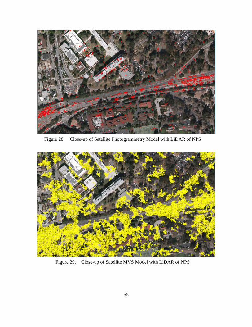
Due to the much higher density of the LiDAR point cloud, it was not meaningful

to render the points in white for the comparisons shown in Figures 28 through 31, so the

LiDAR data was left in true color. The photogrammetry model was changed to red or

purple and the MVS model was rendered in yellow to make visual analysis easier.

The results from the automated photogrammetric analysis were disappointing.

Photogrammetric approaches can clearly produce better results, but more human

intervention may be required. As seen in Figure 28, the red points of the photogrammetry

54

model loosely match the LiDAR data. It was difficult to align the two models because of

the sparse number of photogrammetry points but the highway was used as a constant

across the 12-year span between datasets. Once the road had been lined up the lack of

coherence between man-made structures became quite obvious as the photogrammetry

model failed to outline buildings and only a few continuous surfaces can be found. The

eATE module of IMAGINE Photogrammetry was utilized both with and without

manually entered tie points in hopes of improving the result but the outcomes were nearly

identical. The unexpectedly poor result may be due to the temporal span between the

satellite images which is nearly two years. Other factors may include the method of

output, as .las files are not usual photogrammetric products.

The MVS model seen in Figure 29 covers more features than the photogrammetry

model but only about half of it is visible. After a mean ground level had been identified

within the MVS model, it was aligned with the LiDAR and about 50 percent of the points

fell below said level. This is more clearly demonstrated in Figures 30 and 31. The vertical

errors of the two models are equally poor, indicating neither should be utilized further

unless corrections are made.

55

Figure 28. Close-up of Satellite Photogrammetry Model with LiDAR of NPS

Figure 29. Close-up of Satellite MVS Model with LiDAR of NPS

56

Figure 30. Horizontal View of Satellite Photogrammetry Model with LiDAR of NPS

Figure 31. Horizontal View of Satellite MVS Model with LiDAR of NPS

57

Figure 32 more clearly illustrates the inconsistent elevation values provided by

the photogrammetry and MVS software. The purple points range as far as 100 units from

the LiDAR data and the yellow points range as much as 80 units, confirming the software

packages were not meant to handle satellite data.

Figure 32. Transects of Glasgow Hall Models Using Satellite Imagery, Top: Northwest to Southeast, Bottom: Southwest to Northeast

58


59

V. SUMMARY AND CONCLUSION

This research revealed the capabilities of two software packages in creating point

cloud models from both aerial and satellite imagery. Images included those taken with

Hasselblad and UltraCam Eagle digital cameras as well as four satellites: IKONOS,

Worldview-1, Quickbird-1, and GeoEye-1. A LiDAR dataset collected by WSI at a point

density of 30 points/m2 constituted the ground truth which the imagery point clouds were

measured against.

In the aerial imagery MVS trials it was found that when combining three different

datasets of the same location, Glasgow Hall on the NPS campus, the best model was not

necessarily the one with the most images. A single dataset, six photographs collected by

WSI, that provided unique views produced a more complete model of Glasgow Hall than

the combined model with twelve images. It was determined in the third trial that within a

single image dataset results improve when more images are included.

The satellite imagery MVS trial was less conclusive as there were only seven

available images of the Monterey Peninsula from four satellites offering different

resolutions. The results indicated that improvements occurred between each run without

any obvious digression so further work must be completed to determine the ideal number

of satellite images to be included.

On the photogrammetry side, the aerial imagery produced very accurate results.

While some relief displacement occurred due to the angles of the two images used and

holes existed anywhere homogenous surfaces disallowed point registration, the points

that were created as part of this model represented the most truthful elevation values.

Unlike the MVS aerial model which rounded some of the buildings’ walls, the

photogrammetry point cloud stayed true to shape.

When comparing the satellite photogrammetric and MVS models it was found

that neither was accurate enough to use at present. Viewing them horizontally, the MVS

model registered the most points by far while the photogrammetric model contained so

few points it was difficult to identify anything other than a stretch of road and a few

60

building roofs. The spread of z values was so high in both models we conclude these

software packages were not created to work with satellite data as their vertical data were

invalid.

According to these tests LiDAR remains the model of choice due to its accurate

elevation values. Software packages utilizing aerial imagery have improved to the point

that models indicating the general shape and location of objects are possible, even

including building walls and vertical structures. On the other hand, satellite imagery

products require more rigorous algorithms to ground points to surfaces before they can be

of further use.

Subsequent research should focus on overcoming software weaknesses in

analyzing satellite imagery. If vertical data could be correctly determined, satellite

models could be used to represent much larger areas in less time. Further research into

other software packages might also reveal capabilities not found in those studied here.

61

LIST OF REFERENCES

Aerial Photography. (2013). In J. Hannavy (Ed.), Encyclopedia of nineteenth-century photography (p. 13). London: Routledge.

Agarwal, S., Furukawa, Y., Snavely, N., Simon, I., Curless, B., Seitz, S. M., & Szeliski, R. (2011). Building Rome in a day. Communications of the ACM, 54(10), 105–112. doi: 10.1145/2001269.2001293

Bagley, J. (1917). The use of the panoramic camera in topographic surveying. Washington DC: Government Printing Office.

Basgall, P. (2013). LiDAR point cloud and stereo image point cloud fusion (master’s thesis). Retrieved from Calhoun: http://hdl.handle.net/10945/37584

Church, E., & Quinn, A. (1948). Elements of Photogrammetry. Syracuse, NY: Syracuse University Press.

Diaz, J. C. F. (2011). Lifting the Canopy Veil: Airborne LiDAR for Archaeology of Forested Areas. Imaging Notes, 26(2) , 31–34.. Retrieved from http://www.imagingnotes.com/go/article_freeJ.php?mp_id=264

Digital Wisdom [Image]. (2014). Retrieved from https://www.digiwis.com/dwi_uss.htm

Digital Globe. (2013). Data sheets for IKONOS, GeoEye-1, Worldview-1, and Quickbird 2. Retrieved from http://www.digitalglobe.com/resources/satellite-information

Dismukes, K. (2005). Space Shuttle basics, human space flight. Retrieved from http://spaceflight.nasa.gov/shuttle/reference/basics

Early Techniques and Equipment [Image]. (2000). Retrieved September 5, 2014 from https://airandspace.si.edu/exhibitions/looking-at-earth/online/script/ss_early2.htm

Eisert, P., Steinbach, E., & Girod, B. (1999). Multi-hypothesis, volumetric reconstruction of 3-D objects from multiple calibrated camera views. In Proceedings of the 1999 IEEE International Conference on Acoustics, Speech, and Signal Processing, 6, pp. 3509–3512. IEEE. doi: 10.1109/ICASSP.1999.757599

Erdkamp, J. (2011). Theodor Scheimpflug: The life and work of the man who gave us that rule. Photohistorisch Tijdschrift/Photo-Historical Journal, 34,3. Retrieved from http://kodaksefke.eu/scheimpflug-file.html

Erdkamp, J. (2011). The Theodor Scheimpflug file. Retrieved from http://kodaksefke.eu/scheimpflug-file.html.

62

Faugeras, O., & Keriven, R. (2002). Variational principles, surface evolution, PDE’s, level set methods and the stereo problem. In Proceedings of the 5th European Conference on Computer Vision, pp. 379–393. doi: 10.1109/SSBI.2002.1233990

Furukawa, Y., & Ponce, J. (2010). Accurate, dense, and robust multiview stereopsis. IEEE Transactions on Pattern Analysis and Machine Intelligence, 32(8), pp. 1362–1376. doi: 10.1109/TPAMI.2009.161

Gargallo, P., & Sturm, P. (2005). Bayesian 3D modeling from images using multiple depth maps. In Proceedings of the IEEE Computer Society Conference on Computer Vision and Pattern Recognition, 2, pp. 885–891. IEEE. doi: 10.1109/CVPR.2005.84

Guerra, F., & Pilot, L. (2000). Historic photoplanes. In International Archives of Photogrammetry and Remote Sensing, XXXIII(B5), 611–618. Retrieved from http://www.isprs.org/proceedings/xxxiii/congress/part5/611_XXXIII-part5.pdf

Hartley, R. I., & Mundy, J. L. (1993). The relationship between photogrammetry and computer vision. In Optical engineering and photonics in aerospace sensing, pp. 92–105. International Society for Optics and Photonics.

Hirschmuller, H. (2005). Accurate and efficient stereo processing by semi-global matching and mutual information. In Proceedings of the IEEE Computer Society Conference on Computer Vision and Pattern Recognition, 2, pp. 807–814. IEEE. doi: 10.1109/CVPR.2005.56

Hirschmüller, H. (2011). Semi-global matching motivation, developments and applications. Photogrammetric Week, 53, 173–184. Retrieved from http://www.ifp.uni-stuttgart.de/publications/phowo11/180Hirschmueller.pdf

Image-based measurements in machine vision: technology hints [Image]. (2008). Retrieved from http://cvg.deis.unibo.it/technology_hints_en.html

Laussedat, Aimé. (1899). La Métrophotographie. Paris, France: Gauthier-Villars, Imprimeur-Libraire. Retrieved from http://becot.info/opus/analecta/Laussedat_Metrophotographie1899.pdf

Laussedat, Aimé. (2008). In Complete dictionary of scientific biography. Retrieved from http://www.encyclopedia.com/doc/1G2-2830902500.html

Lindeberg, T. (2012). Scale invariant feature transform. In Scholarpedia. Retrieved from http://www.scholarpedia.org/article/Scale_Invariant_Feature_Transform# Extensions

Merklinger, H. (1996). Scheimpflug’s patent. Photo Technique. Retrieved from http://www.trenholm.org/hmmerk/HMArtls.html

63

Moffitt, F. (1959). Photogrammetry. Scranton, PA: International Textbook Company.

Morris, D., & Kanade, T. (2000). Image-consistent surface triangulation. In Proceedings of the IEEE Computer Society Conference on Computer Vision and Pattern Recognition, 1, pp. 332–338. IEEE. doi: 10.1109/CVPR.2000.855837

NPS Statistics [Image]. (2014). Retrieved from www.nps.edu/About/NPS_Statistics

Old Delft Scanning Stereoscope [Image]. (2009). Retrieved from http://www.publicsurplus.com/sms/auction/view?auc=310310

Quam, L. H. (1971). Computer comparison of pictures (No. STAN-CS-71-219). Stanford Univ CA Dept Of Computer Science. Retrieved from http://www.dtic.mil/cgi-bin/GetTRDoc?AD=AD0785172

Rosenfeld, A. (1969). Picture processing by computer. ACM Computing Surveys (CSUR), 1(3), 147–176. doi: 10.1145/356551.356554

Saiz, Angel. (2012). Nadar. Retrieved from http://historiasdearteyguerra.blogspot.com/2012/09/nadar.html

Schuckman, K., & Renslow, M. (2014). Ground-based platforms. Pennsylvania State University: John A. Dutton e-Education Institute. Retrieved from https://www.e-education.psu.edu/lidar/l2_p5.html

Seitz, S. M., Curless, B., Diebel, J., Scharstein, D., & Szeliski, R. (2006). A comparison and evaluation of multi-view stereo reconstruction algorithms. In IEEE Computer Society Conference on Computer vision and pattern recognition, 1, pp. 519–528. IEEE. doi: 10.1109/CVPR.2006.19

Seitz, S. M. & Dyer, C. R. (1999). Photorealistic Scene Reconstruction by Voxel Coloring. International Journal of Computer Vision, 35(2), pp. 151–173. doi: 10.1023/A:1008176507526

Shan, J., & Toth, C. K. (2009). Topographic laser ranging and scanning: Principles and processing. Boca Raton, FL: CRC Press/Taylor & Francis Group.

Shepherd, E. (2006). Il rilievo topofotografico di Ostia dal pallone 1911. In Archeologia Aerea Studi di Aerotopografia Archeologica, 2, pp. 15–38. Retrieved from http://www.ostia-antica.org/fulltext/shepherd/shepherd_aaerea.pdf

Tardivo, C. (1911). Manuale di fotografia-telefotografia, topofotografia dal pallone. Torina.

Total station and its applications in surveying [Image]. n.d. Retrieved September 3, 2014 from http://www.gisresources.com/total-station-and-its-applications-in-surveying

64

University of Texas at Austin (2013). Monterey Naval Postgraduate School Data Collect. Austin, TX: University of Texas.

Van Gool, L., Tuytelaars, T., Ferrari, V., Strecha, C., Wyngaerd, J. V., & Vergauwen, M. (2002). 3D modeling and registration under wide baseline conditions. International Archives of Photogrammetry and Remote Sensing, 34(3A), 3–14.

Watershed Sciences, I. (2012). Monterey Naval Postgraduate School Data Collect. Portland, Oregon: Watershed Sciences, Inc.

Walker, S. (2007). New features in SOCET SET®. Photogrammetric Week, 49(7), 35–40. Retrieved from http://www.ifp.uni-stuttgart.de/publications/phowo07/060Walker.pdf

65

INITIAL DISTRIBUTION LIST

1. Defense Technical Information Center Ft. Belvoir, Virginia 2. Dudley Knox Library Naval Postgraduate School Monterey, California

naval postgraduate school · author amanda r. mueller 7. performing organization name(s) and...

Documents