naval postgraduate school · report documentation page ... pollard’s kangaroo algorithm ... my...

NAVAL

POSTGRADUATE SCHOOL

MONTEREY, CALIFORNIA

THESIS

Approved for public release; distribution is unlimited

AN ANALYSIS OF ALGORITHMS FOR SOLVING DISCRETE LOGARITHMS IN FIXED GROUPS

by

Joseph Mihalcik

March 2010

Thesis Advisor: Dennis Volpano Second Reader: Harold Fredricksen

i

REPORT DOCUMENTATION PAGE Form Approved OMB No. 0704-0188 Public reporting burden for this collection of information is estimated to average 1 hour per response, including the time for reviewing instruction, searching existing data sources, gathering and maintaining the data needed, and completing and reviewing the collection of information. Send comments regarding this burden estimate or any other aspect of this collection of information, including suggestions for reducing this burden, to Washington headquarters Services, Directorate for Information Operations and Reports, 1215 Jefferson Davis Highway, Suite 1204, Arlington, VA 22202-4302, and to the Office of Management and Budget, Paperwork Reduction Project (0704-0188) Washington DC 20503. 1. AGENCY USE ONLY (Leave blank)

2. REPORT DATE March 2010

3. REPORT TYPE AND DATES COVERED Master’s Thesis

4. TITLE AND SUBTITLE An Analysis of Algorithms for Solving Discrete Logarithms in Fixed Groups 6. AUTHOR(S) Joseph Mihalcik

5. FUNDING NUMBERS

7. PERFORMING ORGANIZATION NAME(S) AND ADDRESS(ES) Naval Postgraduate School Monterey, CA 93943-5000

8. PERFORMING ORGANIZATION REPORT NUMBER

9. SPONSORING /MONITORING AGENCY NAME(S) AND ADDRESS(ES) Department of Defense

10. SPONSORING/MONITORING AGENCY REPORT NUMBER

11. SUPPLEMENTARY NOTES The views expressed in this thesis are those of the author and do not reflect the official policy or position of the Department of Defense or the U.S. Government.

12a. DISTRIBUTION / AVAILABILITY STATEMENT Approved for public release; distribution is unlimited

12b. DISTRIBUTION CODE

13. ABSTRACT (maximum 200 words) Internet protocols such as Secure Shell and Internet Protocol Security rely on the assumption that finding discrete logarithms is hard. The protocols specify fixed groups for Diffie-Hellman key exchange that must be supported. Although the protocols allow flexibility in the choice of group, it is highly likely that the specific groups required by the standards will be used in most cases. There are security implications to using a fixed group, because solving any discrete logarithm within a group is comparatively easier after a group-specific precomputation has been completed. In this work, we more accurately model real-world cryptographic applications with fixed groups. We use an analysis of algorithms to place an upper bound on the complexity of solving discrete logarithms given a group-specific precomputation.

15. NUMBER OF PAGES

71

14. SUBJECT TERMS Discrete Logarithms, Analysis of Algorithms, Advice Strings, Diffie-Hellman Key Exchange

16. PRICE CODE

17. SECURITY CLASSIFICATION OF REPORT

Unclassified

18. SECURITY CLASSIFICATION OF THIS PAGE

Unclassified

19. SECURITY CLASSIFICATION OF ABSTRACT

Unclassified

20. LIMITATION OF ABSTRACT

UU NSN 7540-01-280-5500 Standard Form 298 (Rev. 2-89) Prescribed by ANSI Std. 239-18

ii

THIS PAGE INTENTIONALLY LEFT BLANK

iii

Approved for public release; distribution is unlimited

AN ANALYSIS OF ALGORITHMS FOR SOLVING DISCRETE LOGARITHMS IN FIXED GROUPS

Joseph P. Mihalcik

Civilian, Department of Defense B.S., University of Maryland, College Park, 2000

Submitted in partial fulfillment of the requirements for the degree of

MASTER OF SCIENCE IN COMPUTER SCIENCE

from the

NAVAL POSTGRADUATE SCHOOL March 2010

Author: Joseph P. Mihalcik

Approved by: Dennis Volpano Thesis Advisor

Harold Fredricksen Second Reader

Peter Denning Chairman, Department of Computer Science


iv

ABSTRACT

Internet protocols such as Secure Shell and Internet Protocol Security rely on the as-sumption that finding discrete logarithms is hard. The protocols specify fixed groups for Diffie-Hellman key exchange that must be supported. Although the protocols allow flexibility in thechoice of group, it is highly likely that the specific groups required by the standards will beused in most cases. There are security implications to using a fixed group, because solving anydiscrete logarithm within a group is comparatively easier after a group-specific precomputationhas been completed. In this work, we more accurately model real-world cryptographic appli-cations with fixed groups. We use an analysis of algorithms to place an upper bound on thecomplexity of solving discrete logarithms given a group-specific precomputation.

v


vi

TABLE OF CONTENTS

I. Introduction 1

II. Background 5A. Discrete Logarithms Explained . . . . . . . . . . . . . . . . . . . . . . . . . . 5

1. Discrete Logarithm Example . . . . . . . . . . . . . . . . . . . . . . . 62. Discrete Logarithm Problem . . . . . . . . . . . . . . . . . . . . . . . 6

B. Cryptography and Discrete Logarithms . . . . . . . . . . . . . . . . . . . . . . 71. Diffie-Hellman Key Agreement . . . . . . . . . . . . . . . . . . . . . 82. ElGamal . . . . . . . . . . . . . . . . . . . . . . . . . . . . . . . . . 93. Digital Signature Algorithm . . . . . . . . . . . . . . . . . . . . . . . 11

C. Fixed Groups in Cryptographic Protocols . . . . . . . . . . . . . . . . . . . . 131. Groups in SSH . . . . . . . . . . . . . . . . . . . . . . . . . . . . . . 142. Groups in IKE . . . . . . . . . . . . . . . . . . . . . . . . . . . . . . 143. Advantages of Fixed Groups . . . . . . . . . . . . . . . . . . . . . . . 154. Risks of Using Fixed Groups . . . . . . . . . . . . . . . . . . . . . . . 16

III.Survey of Discrete Logarithm Algorithms 19A. Generic vs. Group-Specific Algorithms . . . . . . . . . . . . . . . . . . . . . 19B. Model of Computation . . . . . . . . . . . . . . . . . . . . . . . . . . . . . . 20C. Brute-Force Search . . . . . . . . . . . . . . . . . . . . . . . . . . . . . . . . 21D. Precomputed Table Algorithm . . . . . . . . . . . . . . . . . . . . . . . . . . 21E. Shank’s Algorithm . . . . . . . . . . . . . . . . . . . . . . . . . . . . . . . . 22F. Pohlig-Hellman Algorithm . . . . . . . . . . . . . . . . . . . . . . . . . . . . 24G. Pollard’s Rho Algorithm . . . . . . . . . . . . . . . . . . . . . . . . . . . . . 25H. Pollard’s Kangaroo Algorithm . . . . . . . . . . . . . . . . . . . . . . . . . . 28I. Index Calculus Algorithm . . . . . . . . . . . . . . . . . . . . . . . . . . . . . 31J. Summary . . . . . . . . . . . . . . . . . . . . . . . . . . . . . . . . . . . . . 36

IV. Complexity of Discrete Logarithms over Fixed Groups 37A. The Para-Discrete Logarithm Problem . . . . . . . . . . . . . . . . . . . . . . 37B. The Para-Discrete Logarithm Problem with an Advice String . . . . . . . . . . 39C. Para-Discrete Logarithm Algorithms . . . . . . . . . . . . . . . . . . . . . . . 39

1. Brute-Force Search and Precomputed Table Algorithms . . . . . . . . 40

vii

2. Shank’s Algorithm . . . . . . . . . . . . . . . . . . . . . . . . . . . . 403. Pollard’s Rho Algorithm . . . . . . . . . . . . . . . . . . . . . . . . . 424. Pollard’s Kangaroo Algorithm . . . . . . . . . . . . . . . . . . . . . . 445. Index Calculus Algorithm . . . . . . . . . . . . . . . . . . . . . . . . 47

D. Summary . . . . . . . . . . . . . . . . . . . . . . . . . . . . . . . . . . . . . 49

List of References 51

Initial Distribution List 55

viii

LIST OF TABLES

1. Powers of g = 2 in Z∗11 . . . . . . . . . . . . . . . . . . . . . . . . . . . . . . 72. Discrete Logarithms to the base g = 2 in Z∗11 . . . . . . . . . . . . . . . . . . 8

3. Complexity of Discrete Logarithm Algorithms . . . . . . . . . . . . . . . . . . 36

4. Time-Memory Trade-Offs of Para-Discrete Logarithm Algorithms . . . . . . . 495. Complexity of Para-Discrete Logarithm Algorithms . . . . . . . . . . . . . . . 50

ix


x

LIST OF ALGORITHMS AND DEFINITIONS

1. The Discrete Logarithm Problem (DLP) . . . . . . . . . . . . . . . . . . . . . 62. The Generalized Discrete Logarithm Problem (GDLP) . . . . . . . . . . . . . 73. Public Key Encryption (PKE) . . . . . . . . . . . . . . . . . . . . . . . . . . . 104. ElGamal Key Generation . . . . . . . . . . . . . . . . . . . . . . . . . . . . . 105. ElGamal Encryption . . . . . . . . . . . . . . . . . . . . . . . . . . . . . . . 116. ElGamal Decryption . . . . . . . . . . . . . . . . . . . . . . . . . . . . . . . 117. Digital Signature System . . . . . . . . . . . . . . . . . . . . . . . . . . . . . 128. DSA Key Generation . . . . . . . . . . . . . . . . . . . . . . . . . . . . . . . 129. DSA Signature Generation . . . . . . . . . . . . . . . . . . . . . . . . . . . . 1310. DSA Signature Verification . . . . . . . . . . . . . . . . . . . . . . . . . . . . 1311. Brute-Force Search . . . . . . . . . . . . . . . . . . . . . . . . . . . . . . . . 2112. Precomputed Table Algorithm . . . . . . . . . . . . . . . . . . . . . . . . . . 2213. Shank’s Algorithm . . . . . . . . . . . . . . . . . . . . . . . . . . . . . . . . 2314. Pohlig-Hellman Algorithm . . . . . . . . . . . . . . . . . . . . . . . . . . . . 2515. Pollard’s Rho Algorithm . . . . . . . . . . . . . . . . . . . . . . . . . . . . . 2716. Pollard’s Rho - Random Sequence Algorithm . . . . . . . . . . . . . . . . . . 2817. Pollard’s Kangaroo Algorithm . . . . . . . . . . . . . . . . . . . . . . . . . . 2918. Index Calculus Algorithm . . . . . . . . . . . . . . . . . . . . . . . . . . . . . 3319. The Para-Discrete Logarithm Problem (PDLP) . . . . . . . . . . . . . . . . . . 3820. The Generalized Para-Discrete Logarithm Problem (GPDLP) . . . . . . . . . . 3821. Precomputed Table: Advice Generator . . . . . . . . . . . . . . . . . . . . . . 4022. Precomputed Table: Instance Solver . . . . . . . . . . . . . . . . . . . . . . . 4023. Shank’s Algorithm: Advice Generator . . . . . . . . . . . . . . . . . . . . . . 4124. Shank’s Algorithm: Instance Solver . . . . . . . . . . . . . . . . . . . . . . . 4125. Pollard’s Rho Algorithm: Advice Generator . . . . . . . . . . . . . . . . . . . 4326. Pollard’s Rho Algorithm: Instance Solver . . . . . . . . . . . . . . . . . . . . 4427. Pollard’s Kangaroo Algorithm: Advice Generator . . . . . . . . . . . . . . . . 4528. Pollard’s Kangaroo Algorithm: Instance Solver . . . . . . . . . . . . . . . . . 4629. Index Calculus Algorithm: Advice Generator . . . . . . . . . . . . . . . . . . 4830. Index Calculus Algorithm: Instance Solver . . . . . . . . . . . . . . . . . . . . 49

xi


xii

Acknowledgements

Thanks to Jonathan Herzog, Harold Fredricksen, and Dennis Volpano for stimulating,informative discussions and helpful suggestions.

Professor Herzog was the actual primary advisor for this thesis. Unfortunately, I finishedmy thesis after Professor Herzog left the Naval Postgraduate School or his name would officiallyappear as advisor. His continued help in completing the thesis after his professional obligationended is greatly appreciated.

I especially want to thank my wife, Alexandria, and my daughter, Kaitlyn. I never wouldhave been able to finish this without their constant love and support.

xiii


xiv

I. Introduction

Thirty years ago, the field of cryptography was revolutionized when Whitfield Diffieand Martin Hellman published New Directions in Cryptography [3]. In this seminal paper, theyintroduced the idea of public key cryptography, a concept that now provides the foundation forsecure communications and secure financial transactions over the Internet. In the same paper,they also described a method for exchanging secret keys over an insecure network. Now knownas the Diffie-Hellman key exchange, this method is used within common network security pro-tocols including Secure Shell (SSH) [28] and Internet Protocol Security (IPsec) [12].

The Diffie-Hellman key exchange is an application of group theory. Computing the se-cret key requires modular exponentiation: raising a number to an exponent within a group ofintegers modulo a prime number. The inverse operation of modular exponentiation is calledfinding the discrete logarithm. Exponentiation is computationally easy, while finding discretelogarithms is believed to be hard. The key exchange depends on this asymmetry in computa-tional complexity for its security. If an adversary can compute discrete logarithms, the adversarycan break Diffie-Hellman and recover the secret key. This situation has lead to a vast amountof research toward finding efficient algorithms to solve discrete logarithms and also towardsunderstanding the computational complexity of the discrete logarithm problem.

Algorithms solving discrete logarithms generally can be divided into two phases: aprecomputation phase and a search phase. The precomputation phase is run first and the resultis stored in memory. The stored result is used in the search phase to speed up computation ofthe discrete logarithm. Often, the precomputation algorithm requires only the group description.This means that the first phase is independent of any particular instance of a discrete logarithm.Additional discrete logarithms over the same group can be solved by running just the searchphase.

Our work focuses on the efficiency of solving multiple discrete logarithms over the samegroup. The practical importance of this investigation can be seen when we examine how theDiffie-Hellman key exchange is used in real applications, such as the SSH and IPsec security

1

protocols. Within these protocols, a small number of standard groups are defined. For example,the standard for SSH only defines two groups that must be supported. There are valid reasonsto use standard groups. In particular, when two users exchange keys, using a standard grouprelieves one user from the computational burden of creating a secure group and the other userfrom the need to trust that it has been done securely. Choosing a secure group requires avoidingcertain groups with characteristics that make them easier to solve. Leaving group choice to astandards committee saves the user significant computation time, but the result will be manykey exchanges occurring over the same fixed groups. This provides an advantage to the attackerin that the cost of precomputation for a group can now be amortized over many key exchanges.As more exchanges occur under a group, the group precomputation increases in value to anattacker. Therefore, our analysis must take into account an attacker that can dedicate largeparallel systems to the precomputation.

Typically, a security analysis of discrete logarithm cryptography would consider thecomplexity of the discrete logarithm problem (DLP). However, the DLP is an incomplete modelfor cryptographic applications with fixed groups. In these applications, the group is constant,but the DLP treats the group as a variable input to the problem. In the DLP, the problem is tofind a single discrete logarithm in a given group, however, a precomputation provides no bene-fit when solving only one instance. Group-specific precomputation is most valuable when thegroup is reused often, which is the case for standards that specify fixed groups. Current secu-rity proofs based on the DLP do not account for group-specific precomputation and, therefore,underestimate the difficulty of attacking applications that specify fixed groups.

In this work, we present a more conservative security model for fixed groups that showsthat such real-world applications provide less cryptographic strength than previously acknowl-edged. In particular, we introduce the para-discrete logarithm problem (PDLP), a variant of theDLP where the group is not an input, but rather dependent only on the input size. This allows usto model the result of a group-specific precomputation as an advice string. In complexity theory,an advice string is roughly a piece of data provided to a help solve a computational problem,and the data can be dependent on the size of the input, but not on the input itself. In the standardDLP, the precomputation is not an advice string, because it is based on an input: the group.Once the precomputation has been completed for a standard group, the DLP is reduced to ourPDLP with an advice string.

We use an analysis of algorithms to place an upper bound on the complexity of the para-discrete logarithm problem with an advice string. In particular, we provide an analysis of thecommon algorithms for solving discrete logarithms, focusing on the relationship between the

2

asymptotic running times of the two phases and the asymptotic bit-length of the advice string.Given a group of order N , we show that the generalized para-discrete logarithm problem can besolved inO(N1/3) group operations with an advice string of sizeO(N1/3). The precomputationof such an advice string requires O(N2/3) group operations.

The rest of the work is as follows. In the next chapter, we review both the technicalbackground and the prior research in the field of cryptography that is relevant to understandingour work. In Chapter III, we survey the known algorithms for the discrete logarithm problemand perform a traditional analysis of their complexity. In Chapter IV, we consider the complex-ity of discrete logarithms over fixed groups and reanalyze the discrete logarithm algorithms inthat context.

3


4

II. Background

In this chapter, we review both the technical background and the prior research in thefield of cryptography that is relevant to understanding our work. In particular, we begin bydescribing discrete logarithms. Next, we examine their importance in cryptology. Lastly, welook at the use of fixed groups in cryptographic protocols.

A. Discrete Logarithms Explained

In this section, we describe discrete logarithms. In particular, we first relate discretelogarithms to standard logarithms in real numbers. Then, we provide mathematical definitionsfor group exponentiation and discrete logarithms. Next, we provide a simple concrete exampleof discrete logarithms. Lastly, we first define the standard computational problems regardingdiscrete logarithms; that is, the discrete logarithm problem (DLP) and the generalized discretelogarithm problem (GDLP). Throughout, we assume the reader is familiar with the concept ofgroups from abstract algebra.

Discrete logarithms are so named because they are analogous to standard logarithmswith real numbers. Just as the logarithm is the inverse operation of exponentiation, the discretelogarithm is the inverse operation of group exponentiation. In the real numbers, log ga = x ifgx = a. The same is true for discrete logarithms, except g and a are elements of a multiplicativecyclic group, G, with generator g. A cyclic group is a group where all the elements of the groupcan be generated by raising one element, a generator, to successive powers.

Group exponentiation to a power x ∈ N, can be defined as repeated group multiplication,

gx =x∏1

g

Methods such as repeated-squaring [16, Algorithm 2.143] allow group exponentiation to bedone efficiently, with just lg x multiplications. In the group Z∗n , where the group operation is

5

multiplication modulo an integer, n, group exponentiation is called modular exponentiation. Inthis setting, the value of gx is a if and only if gx ≡ a mod n. We can compute gx by raising gto the power x in the integers, then finding the remainder modulo n. (There are more practicalalgorithms as well [8].)

Finding a discrete logarithm means inverting the exponentiation and finding the expo-nent x given the value, a. That is, given g, n, and a, find a value of x, 0 ≤ x < n − 1,such that gx ≡ a mod n. While efficient algorithms exist for group exponentiation, no effi-cient algorithm is known for computing discrete logarithms. This asymmetry is what makesexponentiation useful in public key cryptography.

1. Discrete Logarithm Example

To further clarify, we will use a concrete example in Z∗p . The group Z∗p is the multiplica-tive group of integers modulo a prime, p. The elements of Z∗p are the integers 1, 2, . . . , p − 1.In this example, a is an element of the group that can be represented as a = gx, where xis an integer, 0 ≤ x < p − 1. The discrete logarithm of a to the base g, can be written aslog ga = log gg

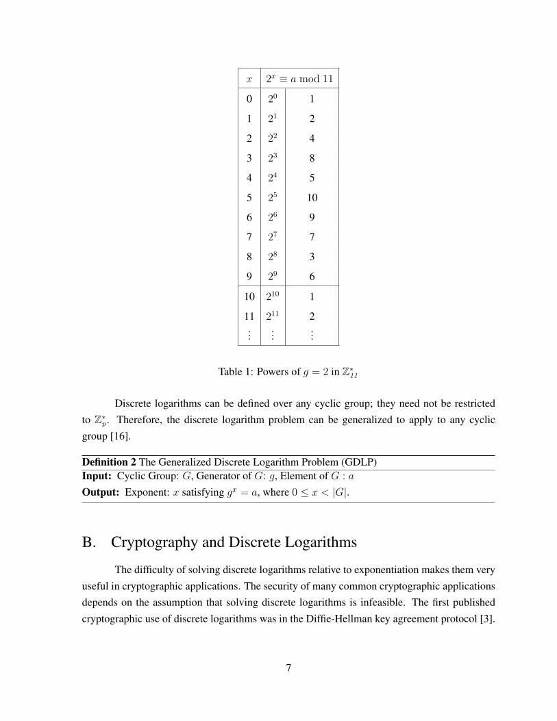
x = x. For this example, if we let p = 11 and g = 2, Table 1 shows the pow-ers of g. If we look in the table at the row x = 4 we see a = gx = 24 = 16 ≡ 5 mod 11.All ten elements of Z∗p are generated before we see another 1 in the table. For every g ∈ Z∗p ,gp−1 ≡ 1 mod p, and, if g is a generator, then there is no element 0 ≤ x < p − 1 such thatgx ≡ 1 mod p. There is no x < 10 such that 2x ≡ 1 mod 11, so 2 is a generator of Z∗11 . Alsonote that the values for greater exponents repeat, 20 = 210 = 1 mod 11.

When we invert this table we have the discrete logarithms in Z∗11 . Table 2 shows us thediscrete logarithms. For example, looking in the table at a = 5 we find log 25 = 4.

2. Discrete Logarithm Problem

Before we can analyze the security of cryptography, it is helpful to formally define thecomputational problems upon which that security relies. The DLP is the problem of solvingdiscrete logarithms over the group of integers modulo a prime and can be formalized as fol-lows [16],

Definition 1 The Discrete Logarithm Problem (DLP)Input: Prime: p, Generator of Z∗p: g, Element of Z∗p: aOutput: Exponent: x satisfying gx ≡ a mod p, where 0 ≤ x < p− 1.

6

x 2x ≡ a mod 11

0 20 1

1 21 2

2 22 4

3 23 8

4 24 5

5 25 10

6 26 9

7 27 7

8 28 3

9 29 6

10 210 1

11 211 2...

......

Table 1: Powers of g = 2 in Z∗11

Discrete logarithms can be defined over any cyclic group; they need not be restrictedto Z∗p . Therefore, the discrete logarithm problem can be generalized to apply to any cyclicgroup [16].

Definition 2 The Generalized Discrete Logarithm Problem (GDLP)Input: Cyclic Group: G, Generator of G: g, Element of G : a

Output: Exponent: x satisfying gx = a, where 0 ≤ x < |G|.

B. Cryptography and Discrete Logarithms

The difficulty of solving discrete logarithms relative to exponentiation makes them veryuseful in cryptographic applications. The security of many common cryptographic applicationsdepends on the assumption that solving discrete logarithms is infeasible. The first publishedcryptographic use of discrete logarithms was in the Diffie-Hellman key agreement protocol [3].

7

a log ga = x

1 log 21 0

2 log 22 1

3 log 23 8

4 log 24 2

5 log 25 4

6 log 26 9

7 log 27 7

8 log 28 3

9 log 29 6

10 log 210 5

Table 2: Discrete Logarithms to the Base g = 2 in Z∗11

The first public key cryptosystem relying on discrete logarithms was the ElGamal cryptosys-tem [4]. ElGamal also developed the first signature scheme based on discrete logarithms, avariant of which is the Digital Signature Algorithm (DSA) [19].

In this section, we present several cryptographic algorithms to demonstrate the practicalimportance of discrete logarithms. In particular, we first examine the Diffie-Hellman key agree-ment scheme. Next, we focus on the public key encryption system known as ElGamal. Finally,we examine the Digital Signature Algorithm (DSA).

1. Diffie-Hellman Key Agreement

The Diffie-Hellman key agreement enables two parties to agree on a secret key over aninsecure channel without revealing the key to an attacker. In this scheme, two participants, Aand B, agree on a cyclic group, G, and generator of the group, g. We must assume the attackerwill know the details of the group, as they will be sent over the same insecure channel. A and Bindependently and randomly choose their own secret exponents, a and b, respectively. User Acomputes and transmits ga; B computes and transmits gb. The secret key they agree on is gab.

8

User A computes the secret key by raising gb (received from B) to the power, a (A’s secret),

(gb)a = gba = gab

Equivalently, user B raises the value ga to the power, b,

(ga)b = gab

Now both users know the secret key, gab, while the attacker has only seen ga and gb.Clearly, however, if the attacker could compute discrete logarithms in the group, G, then theattacker could solve for either a or b and compute the secret key. It is an open question whetherthere is an easier way to find gab than to compute discrete logarithms. This is called the Diffie-

Hellman problem.It should also be noted that the Diffie-Hellman key agreement does not provide authen-

tication. An attacker with the ability to modify and insert messages could be in the middle ofan exchange between users A and B. If this occurs, A and B could unknowingly be sharingkeys with the attacker and not each other. To avoid this attack, Diffie-Hellman must be part ofa larger protocol that provides authentication.

2. ElGamal

The ElGamal cryptosystem is a method of public key encryption (PKE) that is based onDiffie-Hellman [4]. In this subsection, we show that the security of ElGamal is dependent onthe difficulty of finding discrete logarithms. In particular, we begin with a formal definition ofPKE. Then we explain what it means for a PKE to be secure. Next we describe the ElGamalalgorithms. Finally, we demonstrate how the security of ElGamal would be compromised if anefficient discrete logarithm method is discovered.

9

Definition 3 Public Key Encryption (PKE)A public key encryption system [6] is a triple of PPT algorithms (G,E,D) such that,

1. G is a key generation algorithm that on input 1k computes output (e, d).

2. E is an encryption algorithm that on input (1k, e,m) computes output c.

3. D is a decryption algorithm that on input (1k, d, c) computes output m.

where 1k is the security parameter, e is the public encryption key, d is the secret decryption key,m ∈ {0, 1}k is the plaintext message and c ∈ {0, 1}∗ is the encrypted ciphertext such that ifG→ (e, d) then D(E(e,m), d) = m.

The security of a PKE system has been defined in terms of semantic security [6]. Infor-mally, a PKE system is semantically secure if an adversary with access to the encryption key,e, and ciphertext, c, has no more than a negligible advantage in guessing the plaintext over anadversary without acesss to e or c.

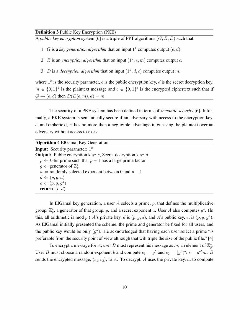
Algorithm 4 ElGamal Key GenerationInput: Security parameter: 1k

Output: Public encryption key: e, Secret decryption key: dp⇐ k-bit prime such that p− 1 has a large prime factorg ⇐ generator of Z∗pa⇐ randomly selected exponent between 0 and p− 1d⇐ (p, g, a)e⇐ (p, g, ga)return (e, d)

In ElGamal key generation, a user A selects a prime, p, that defines the multiplicativegroup, Z∗p , a generator of that group, g, and a secret exponent a. User A also computes ga. (Inthis, all arithmetic is mod p.) A’s private key, d is (p, g, a), and A’s public key, e, is (p, g, ga).As ElGamal initially presented the scheme, the prime and generator be fixed for all users, andthe public key would be only (ga). He acknowledged that having each user select a prime “ispreferable from the security point of view although that will triple the size of the public file.” [4]

To encrypt a message for A, user B must represent his message as m, an element of Z∗p .User B must choose a random exponent b and compute c1 = gb and c2 = (ga)bm = gabm. Bsends the encrypted message, (c1, c2), to A. To decrypt, A uses the private key, a, to compute

10

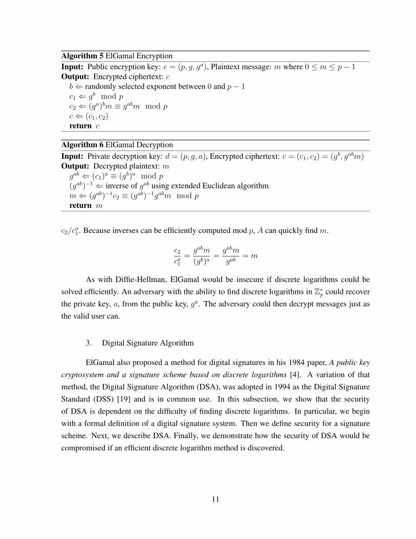
Algorithm 5 ElGamal EncryptionInput: Public encryption key: e = (p, g, ga), Plaintext message: m where 0 ≤ m ≤ p− 1Output: Encrypted ciphertext: cb⇐ randomly selected exponent between 0 and p− 1c1 ⇐ gb mod pc2 ⇐ (ga)bm ≡ gabm mod pc⇐ (c1, c2)return c

Algorithm 6 ElGamal DecryptionInput: Private decryption key: d = (p, g, a), Encrypted ciphertext: c = (c1, c2) = (gb, gabm)Output: Decrypted plaintext: mgab ⇐ (c1)

a ≡ (gb)a mod p(gab)−1 ⇐ inverse of gab using extended Euclidean algorithmm⇐ (gab)−1c2 ≡ (gab)−1gabm mod preturn m

c2/ca1. Because inverses can be efficiently computed mod p, A can quickly find m.

c2ca1

=gabm

(gb)a=gabm

gab= m

As with Diffie-Hellman, ElGamal would be insecure if discrete logarithms could besolved efficiently. An adversary with the ability to find discrete logarithms in Z∗p could recoverthe private key, a, from the public key, ga. The adversary could then decrypt messages just asthe valid user can.

3. Digital Signature Algorithm

ElGamal also proposed a method for digital signatures in his 1984 paper, A public key

cryptosystem and a signature scheme based on discrete logarithms [4]. A variation of thatmethod, the Digital Signature Algorithm (DSA), was adopted in 1994 as the Digital SignatureStandard (DSS) [19] and is in common use. In this subsection, we show that the securityof DSA is dependent on the difficulty of finding discrete logarithms. In particular, we beginwith a formal definition of a digital signature system. Then we define security for a signaturescheme. Next, we describe DSA. Finally, we demonstrate how the security of DSA would becompromised if an efficient discrete logarithm method is discovered.

11

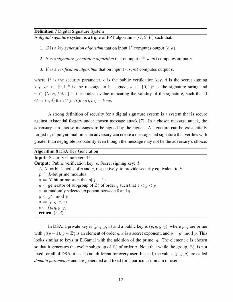
Definition 7 Digital Signature SystemA digital signature system is a triple of PPT algorithms (G,S, V ) such that,

1. G is a key generation algorithm that on input 1k computes output (e, d).

2. S is a signature generation algorithm that on input (1k, d,m) computes output s.

3. V is a verification algorithm that on input (e, s,m) computes output v.

where 1k is the security parameter, e is the public verification key, d is the secret signingkey, m ∈ {0, 1}k is the message to be signed, s ∈ {0, 1}k is the signature string andv ∈ {true, false} is the boolean value indicating the validity of the signature, such that ifG→ (e, d) then V (e, S(d,m),m) = true.

A strong definition of security for a digital signature system is a system that is secureagainst existential forgery under chosen message attack [7]. In a chosen message attack, theadversary can choose messages to be signed by the signer. A signature can be existentiallyforged if, in polynomial time, an adversary can create a message and signature that verifies withgreater than negligible probability even though the message may not be the adversary’s choice.

Algorithm 8 DSA Key GenerationInput: Security parameter: 1k

Output: Public verification key: e, Secret signing key: dL,N ⇐ bit-lengths of p and q, respectively, to provide security equivalent to kp⇐ L-bit prime modulusq ⇐ N -bit prime such that q|(p− 1)g ⇐ generator of subgroup of Z∗p of order q such that 1 < g < px⇐ randomly selected exponent between 0 and qy ⇐ gx mod pd⇐ (p, q, g, x)e⇐ (p, q, g, y)return (e, d)

In DSA, a private key is (p, q, g, x) and a public key is (p, q, g, y), where p, q are primewith q|(p− 1), g ∈ Z∗p is an element of order q, x is a secret exponent, and y = gx mod p. Thislooks similar to keys in ElGamal with the addition of the prime, q. The element g is chosenso that it generates the cyclic subgroup of Z∗p of order q. Note that while the group, Z∗p , is notfixed for all of DSA, it is also not different for every user. Instead, the values (p, q, g) are calleddomain parameters and are generated and fixed for a particular domain of users.

12

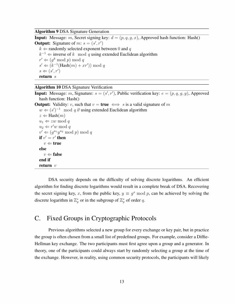
Algorithm 9 DSA Signature GenerationInput: Message: m, Secret signing key: d = (p, q, g, x), Approved hash function: Hash()Output: Signature of m: s = (s′, r′)k ⇐ randomly selected exponent between 0 and qk−1 ⇐ inverse of k mod q using extended Euclidean algorithmr′ ⇐ (gk mod p) mod qs′ ⇐ (k−1(Hash(m) + xr′)) mod qs⇐ (s′, r′)return s

Algorithm 10 DSA Signature VerificationInput: Message: m, Signature: s = (s′, r′), Public verification key: e = (p, q, g, y), Approved

hash function: Hash()Output: Validity: v, such that v = true ⇐⇒ s is a valid signature of mw ⇐ (s′)−1 mod q // using extended Euclidean algorithmz ⇐ Hash(m)u1 ⇐ zw mod qu2 ⇐ r′w mod qv′ ⇐ (gu1yu2 mod p) mod qif v′ = r′ thenv ⇐ true

elsev ⇐ false

end ifreturn v

DSA security depends on the difficulty of solving discrete logarithms. An efficientalgorithm for finding discrete logarithms would result in a complete break of DSA. Recoveringthe secret signing key, x, from the public key, y ≡ gx mod p, can be achieved by solving thediscrete logarithm in Z∗p or in the subgroup of Z∗p of order q.

C. Fixed Groups in Cryptographic Protocols

Previous algorithms selected a new group for every exchange or key pair, but in practicethe group is often chosen from a small list of predefined groups. For example, consider a Diffie-Hellman key exchange. The two participants must first agree upon a group and a generator. Intheory, one of the participants could always start by randomly selecting a group at the time ofthe exchange. However, in reality, using common security protocols, the participants will likely

13

agree to use a group that is specified in their protocol standard.In this section, we look at the use of fixed groups in cryptography. In particular, we first

provide examples of two commonly used cryptographic protocols that define specific groups.These are Secure Shell [29] and Internet Protocol Security [10]. Then, we examine the motiva-tions for specifying fixed groups in protocol standards. Following this, we discuss the securityrisks of reusing groups.

1. Groups in SSH

Protocol standards often specify just a few fixed groups for Diffie-Hellman key ex-changes. The standard for Secure Shell (SSH) [29] only defines two groups. The two pre-defined groups are subgroups of Z∗p where p is a specific 1024-bit prime and a 2048-bit prime,respectively. The primes were selected by a method described in the OAKLEY key determi-nation protocol [20]. In addition to the two required groups, an SSH implementation is free toadd additional groups. But since both client and server implementations must have a specificgroup predefined, this is essentially a mechanism to add additional standard groups. The SSHstandard does not require support for on-the-fly group generation.

There is, however, a proposed Internet standard, Diffie-Hellman Group Exchange for the

Secure Shell (SSH) Transport Layer Protocol [5], that extends SSH to allow new private groups.The standard defines a method for an SSH server to propose a new group to the client. For thisDiffie-Hellman group exchange extension to be effective, it must be supported by implementa-tions and new private groups must actually be created. The popular OpenSSH implements thegroup exchange, but does not automatically generate new groups. Instead, a utility is includedthat allows a server administrator to generate new groups from the command line. Without newgroup generation being automatic and transparent to the user, it is likely that standard groupswill still be used even between implementations supporting this extension.

2. Groups in IKE

The Internet Key Exchange (IKE) [10] is the key exchange protocol used in InternetProtocol Security (IPsec). IKE uses the Diffie-Hellman key exchange and specifies just fourfixed groups. The first two are subgroups of Z∗p where p is a 768-bit prime and 1024-bit primerespectively. The two primes are chosen by the same Oakley method as in SSH. The othertwo standard groups in IKE are a 155-bit and a 185-bit elliptic curve group. The disparity in

14

bit-lengths is because more efficient algorithms are known for solving discrete logarithms inZ∗p groups than in well chosen elliptic curve groups. Therefore a smaller elliptic curve group isbelieved to provide security equivalent to a larger Z∗p group.

3. Advantages of Fixed Groups

There are many valid reasons to specify fixed groups for Diffie-Hellman key exchangesin a protocol standard. In this subsection, we discuss two major advantages of specifying fixedgroups. The first advantage we consider is the reduction in protocol complexity. The secondadvantage we examine is that the standard groups can be carefully selected to be secure, savingthe user the computational expense of creating new secure groups.

Reduced Protocol Complexity

If a protocol is shorter and less complex, its security is easier to analyze and there arefewer opportunities for flaws. A simpler protocol also makes implementation easier with lesschance of errors or incompatibilities with other implementations. Using fixed groups reducesthe protocol complexity. In particular, it eliminates the need to communicate a description ofthe group before the key exchange. Additionally, it eliminates the need for clients to implementa method of secure group selection, which as we see in the next section, can be a complicatedprocess.

Securely Selected Groups

If a group is predefined, it can be carefully selected for desired security properties, andthe selection is not bound by the computational limitations that would exist if the group selectionwas done during a live protocol transaction. A protocol standard must ensure that the keyexchange provides an appropriate level of security, and the security provided by a group dependson more than just bit-length. Certain groups are weak and must be avoided. Specifically, if thegroup order is the product of only small prime factors, discrete logarithms can be computedefficiently in this group [21]. (See Section F on page 24.)

In both SSH and IKE, the groups were selected with the Oakley method to achieve goalsof efficiency, security, and trust that there is no back-door. In particular, for an n-bit prime, p,the Oakley method fixes the first and last 64-bits to all ones to speedup modular exponentiation.Then the interior bits of p are set to (c+m), where c is the first (n− 128) bits of π and m is the

15

smallest positive integer such that p and (p − 1)/2 are both prime. The reason for using π asthe source of randomness is to avoid “any suspicion that the primes have secretly been selectedto be weak” [20].

Additionally, using standard groups eliminates the need for the computationally inten-sive process of group creation within the protocol. Creating a new group requires finding aprime, p, and a generator, g of Z∗p . No efficient method is known for finding a generator of Z∗pfor a random prime, p. This is because efficiently determining that a number is a generator re-quires knowing the factorization of p−1, the order of the group, and factorization is believed tobe a hard problem. Therefore, instead of first choosing a random p, we must generateN = p−1

with a known factorization and then test that p is a prime.To avoid creating a weak group, we want N to have a large prime factor. (Again, see

Section F on page 24.) Because N is even, our best case is if N = 2q for q prime. Thus,to create a secure group Z∗p , we must select random primes, qi, until p = 2qi + 1 is prime.Many iterations of primality testing make this a computationally intensive process. If this hadto be done at the start of each transaction, the user may find the long delay unacceptable. If thegroup creation was performed automatically on the server it could potentially enable a denial ofservice attack.

4. Risks of Using Fixed Groups

The downside of using a fixed group is that it places a high premium on attacking asingle group. There will be many key exchanges over the same group over many years. To anadversary, the value of solving all discrete logarithms over this fixed group will be much higherthan the value of solving all discrete logarithms over a random group that may be used onlyonce. For example, while the value of decrypting a single bank transaction may be small, thevalue of attacking many simultaneously would be great.

The computational cost of computing multiple logarithms in a single group is much lessthan computing the same number of logarithms in separate groups. This is because algorithmsto find discrete logarithms often require a precomputation dependent only on the group. Oncethe precomputation is complete for a group, finding additional discrete logarithms in that groupis comparatively easy.

Using fixed groups also allows the time-consuming precomputation to occur before aspecific key-exchange occurs. Consider a hypothetical attack where the precomputation takesone year, but then solving each instance takes just one hour. (The attacker can trade off instance-

16

time for precomputation-time, so such a disparity is not unreasonable.) Given a random group,the adversary would always take one year from key exchange to solving the key. However, oncean adversary has completed the precomputation for a standard group, a key in that group couldbe solved just one hour after the exchange occurs. If the encrypted information is only valuableto the attacker for a short period of time, only the second attack is worthwhile.

17


18

III. Survey of Discrete Logarithm Algorithms

In this chapter, we survey the known algorithms for solving discrete logarithms andperform a traditional analysis of their complexity. In particular, we begin by distinguishingbetween generic algorithms, which work in all cyclic groups, and group-specific algorithms,which apply only in certain families of groups. Then we define the model of computation onwhich we will base our analysis. After that, we survey several generic algorithms. Lastly, weconsider the index calculus algorithm, which is group-specific. For each algorithm we find theasymptotic running time and space requirements.

A. Generic vs. Group-Specific Algorithms

There are several known algorithms for solving discrete logarithms. In this section, wedivide the algorithms into two categories, generic algorithms and group-specific algorithms.The first category we call generic algorithms, because they apply generally over any type ofcyclic group. A generic algorithm solves the generalized discrete logarithm problem (GDLP).The second category of algorithms are the group-specific algorithms. These are specializedalgorithms that make use of the structure in the group elements and apply only within certainfamilies of groups.

The generic algorithms we will consider include Shank’s algorithm [16], which is alsocalled the Baby-Step Giant-Step algorithm, Pollard’s Rho and Pollard’s Kangaroo algorithms [22].These algorithms apply over any cyclic group including elliptic curve groups and subgroups ofZ∗p , where better methods do not apply. The group-specific algorithms we discuss are index

calculus algorithms. They apply in Z∗p . Therefore, index calculus algorithms solve the standarddiscrete logarithm problem (DLP).

19

B. Model of Computation

In this section, we define our model of computation. In particular, we begin by definingthe abstract machine that which will execute the algorithms. Then we define the notation usedin our analysis. Finally, we explain the format we will use for our analysis of each algorithm.

For our analysis of algorithms to be consistent we need to define a model of computation.Central to that is defining a standard abstract machine for finding the asymptotic running timeof each algorithm. Our model uses a multitape Turing machine, which is a good model ofa standard computer. We provide our runtime complexity in terms of the number of groupoperations. We do this because the complexity of the group operation varies among differentgroup families.

Now we define the standard notation we use in our analysis. For each algorithm, wehave a cyclic group G and a generator g of that group. We let N be the order of g,

N = |〈g〉|,

and let n be the bit-length of N ,2n−1 ≤ N < 2n,

n = dlog2Ne.

When describing the asymptotic performance of these algorithms, we do so in terms of n, asis common practice. In terms of storage, we assume that elements of G can be represented inO(n) bits. This assumption is reasonable because there are less than 2n elements in G.

In the following sections, we perform a traditional complexity analysis of several knownalgorithms for solving discrete logarithms. Each analysis will follow a standard format. Foreach algorithm we begin with a description of the algorithm itself. Next, we analyze the algo-rithm’s runtime complexity. Then we analyze the asymptotic space requirements of the algo-rithm. We conclude the chapter with a table summarizing the space and runtime complexity ofeach algorithm.

20

C. Brute-Force Search

We begin our survey of generic algorithms, with the simplest method, brute-force orexhaustive search. That is simply trying every possible exponent (g0, g1, g2, ...) until a match isfound.

Algorithm 11 Brute-Force SearchInput: Cyclic Group: G, Generator: g, Group Element: aOutput: Exponent: x such that gx = a

1: b⇐ 12: x⇐ 03: while a 6= b do4: b⇐ b× g5: x⇐ x+ 16: end while7: return x

In the worst case, where a = gN−1, every exponent would be tested, requiring a totalof N tests. In terms of the bit-length of the input, n, this requires 2n group operations andcomparisons in the worst case. In the average case, one can expect to find the correct exponentafter searching half the space, or 2n−1 group operations. In either case, the running time of thealgorithm is exponential, O(2n), and will quickly become intractable for increasing n.

On the other hand, the space requirements are minimal. At each step we need only tostore x and b, and both can be represented in n bits. Therefore, the asymptotic space requirementof the brute-force algorithm is O(n).

D. Precomputed Table Algorithm

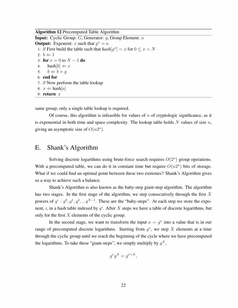
Just two average-case runs of the brute-force search algorithm requires an amount ofwork equivalent to computing all N exponents. Consider, instead, if one first computed all Nexponents and stored them. That is the idea behind our next algorithm, the precomputed tablealgorithm. We build a table holding every discrete logarithm for the group. After computingthe table, finding an individual discrete logarithm requires just a single table lookup.

The running time of the algorithm is dominated by the precomputation, which requiresN group operations. The asymptotic running time of the precomputed table algorithm isO(2n).The advantage of the algorithm is the instant solutions of subsequent discrete logarithms in the

21

Algorithm 12 Precomputed Table AlgorithmInput: Cyclic Group: G, Generator: g, Group Element: aOutput: Exponent: x such that gx = a

1: // First build the table such that hash[gx] = x for 0 ≤ x < N2: b⇐ 13: for x = 0 to N − 1 do4: hash[b]⇐ x5: b⇐ b× g6: end for7: // Now perform the table lookup8: x⇐ hash[a]9: return x

same group; only a single table lookup is required.Of course, this algorithm is infeasible for values of n of cryptologic significance, as it

is exponential in both time and space complexity. The lookup table holds N values of size n,giving an asymptotic size of O(n2n).

E. Shank’s Algorithm

Solving discrete logarithms using brute-force search requires O(2n) group operations.With a precomputed table, we can do it in constant time but require O(n2n) bits of storage.What if we could find an optimal point between these two extremes? Shank’s Algorithm givesus a way to achieve such a balance.

Shank’s Algorithm is also known as the baby-step giant-step algorithm. The algorithmhas two stages. In the first stage of the algorithm, we step consecutively through the first Xpowers of gi : g0, g1, g2, ...gX−1. These are the “baby-steps”. At each step we store the expo-nent, i, in a hash table indexed by gi. After X steps we have a table of discrete logarithms, butonly for the first X elements of the cyclic group.

In the second stage, we want to transform the input a = gx into a value that is in ourrange of precomputed discrete logarithms. Starting from gx, we step X elements at a timethrough the cyclic group until we reach the beginning of the cycle where we have precomputedthe logarithms. To take these “giant-steps”, we simply multiply by gX ,

gxgX = gx+X ,

22

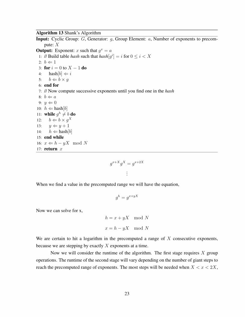
Algorithm 13 Shank’s AlgorithmInput: Cyclic Group: G, Generator: g, Group Element: a, Number of exponents to precom-

pute: XOutput: Exponent: x such that gx = a

1: // Build table hash such that hash[gi] = i for 0 ≤ i < X2: b⇐ 13: for i = 0 to X − 1 do4: hash[b]⇐ i5: b⇐ b× g6: end for7: // Now compute successive exponents until you find one in the hash8: b⇐ a9: y ⇐ 0

10: h⇐ hash[b]11: while gh 6= b do12: b⇐ b× gX13: y ⇐ y + 114: h⇐ hash[b]15: end while16: x⇐ h− yX mod N17: return x

gx+XgX = gx+2X

...

When we find a value in the precomputed range we will have the equation,

gh = gx+yX

Now we can solve for x,h = x+ yX mod N

x = h− yX mod N

We are certain to hit a logarithm in the precomputed a range of X consecutive exponents,because we are stepping by exactly X exponents at a time.

Now we will consider the runtime of the algorithm. The first stage requires X groupoperations. The runtime of the second stage will vary depending on the number of giant steps toreach the precomputed range of exponents. The most steps will be needed when X < x < 2X ,

23

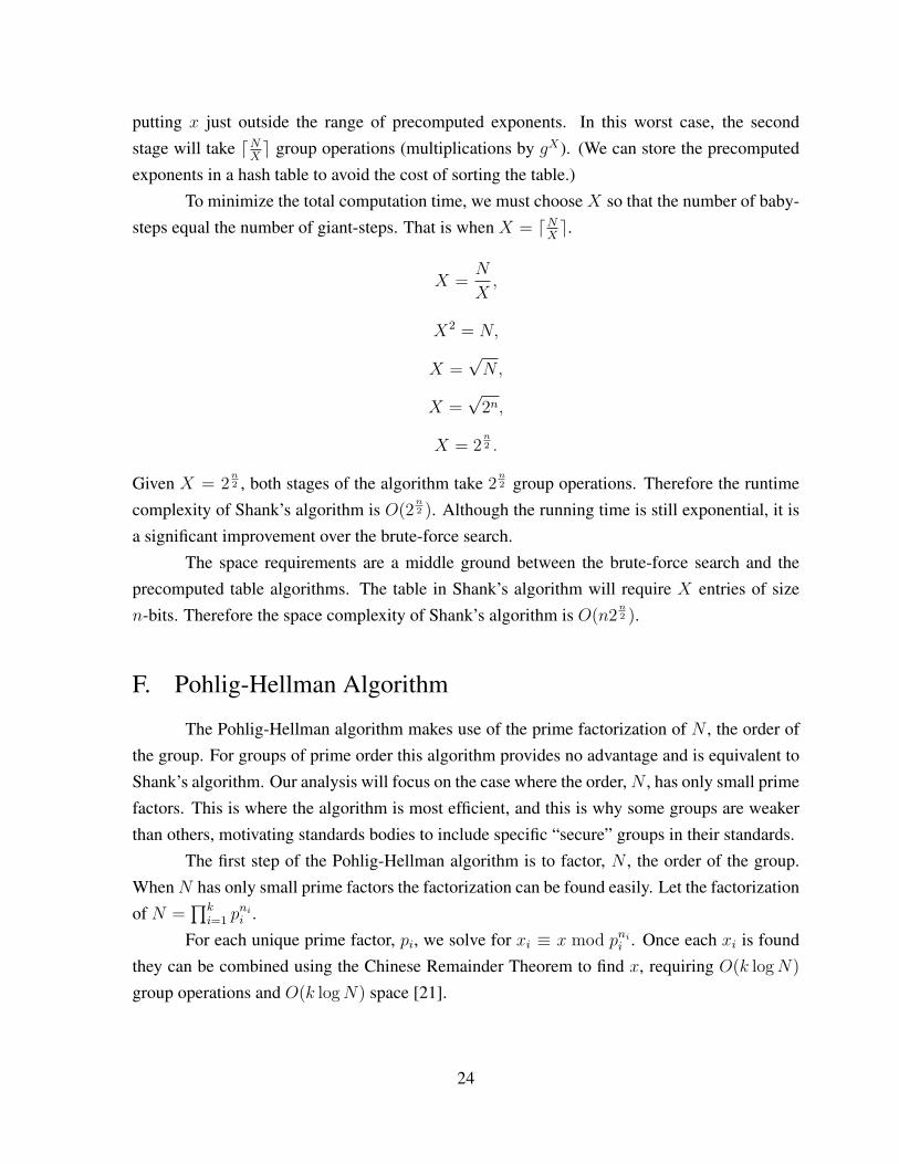
putting x just outside the range of precomputed exponents. In this worst case, the secondstage will take dN

Xe group operations (multiplications by gX). (We can store the precomputed

exponents in a hash table to avoid the cost of sorting the table.)To minimize the total computation time, we must choose X so that the number of baby-

steps equal the number of giant-steps. That is when X = dNXe.

X =N

X,

X2 = N,

X =√N,

X =√

2n,

X = 2n2 .

Given X = 2n2 , both stages of the algorithm take 2

n2 group operations. Therefore the runtime

complexity of Shank’s algorithm is O(2n2 ). Although the running time is still exponential, it is

a significant improvement over the brute-force search.The space requirements are a middle ground between the brute-force search and the

precomputed table algorithms. The table in Shank’s algorithm will require X entries of sizen-bits. Therefore the space complexity of Shank’s algorithm is O(n2

n2 ).

F. Pohlig-Hellman Algorithm

The Pohlig-Hellman algorithm makes use of the prime factorization of N , the order ofthe group. For groups of prime order this algorithm provides no advantage and is equivalent toShank’s algorithm. Our analysis will focus on the case where the order,N , has only small primefactors. This is where the algorithm is most efficient, and this is why some groups are weakerthan others, motivating standards bodies to include specific “secure” groups in their standards.

The first step of the Pohlig-Hellman algorithm is to factor, N , the order of the group.WhenN has only small prime factors the factorization can be found easily. Let the factorizationof N =

∏ki=1 p

nii .

For each unique prime factor, pi, we solve for xi ≡ x mod pnii . Once each xi is found

they can be combined using the Chinese Remainder Theorem to find x, requiring O(k logN)

group operations and O(k logN) space [21].

24

Algorithm 14 Pohlig-Hellman AlgorithmInput: Cyclic Group: G, Generator: g, Group Element: a, Order of group: NOutput: Exponent: x such that gx = a

1: Find the factorization of N =∏k

i=1 pnii

2: // For each factor pnii find xi ≡ x mod pni

i

3: for i = 1 to k do4: z ⇐ a5: h⇐ g−1

6: q ⇐ (p− 1)/pi7: gi ⇐ gq

8: for j = 0 to (ni − 1) do9: w ⇐ zq

10: bj ⇐ loggiw // Solve this discrete logarithm using Algorithm 13

11: z ⇐ zhbj

12: h⇐ hpi

13: q ⇐ q/pi14: end for15: xi ⇐

∑j bjp

ji

16: end for17: Solve for x given x1, ...xk using the Chinese Remainder Theorem18: return x

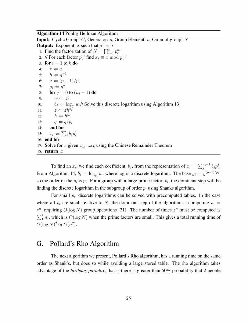
To find an xi, we find each coefficient, bj , from the representation of xi =∑ni−1

j bjpji .

From Algorithm 14, bj = loggiw, where log is a discrete logarithm. The base gi = g(p−1)/pi ,

so the order of the gi is pi. For a group with a large prime factor, pi, the dominant step will befinding the discrete logarithm in the subgroup of order pi using Shanks algorithm.

For small pi, discrete logarithms can be solved with precomputed tables. In the casewhere all pi are small relative to N , the dominant step of the algorithm is computing w =

zn, requiring O(logN) group operations [21]. The number of times zn must be computed is∑k1 ni, which is O(logN) when the prime factors are small. This gives a total running time of

O(logN)2 or O(n2).

G. Pollard’s Rho Algorithm

The next algorithm we present, Pollard’s Rho algorithm, has a running time on the sameorder as Shank’s, but does so while avoiding a large stored table. The rho algorithm takesadvantage of the birthday paradox; that is there is greater than 50% probability that 2 people

25

out of 23 chosen randomly will share a birthday. More generally, when selecting elements atrandom from N elements, a collision will be found after an expected

√πN/2 selections [27].

To find the discrete logarithm of an element a to the base g, Pollard’s Rho algorithmsteps through a random sequence of group elements si that can be represented as products ofpowers of a and g.

si = aaiggi = gxaiggi = gxai+gi .

The algorithm searches for a cycle in the sequence, two elements su, sv, u 6= v such that su = sv.Solving this equation for x gives the discrete logarithm of a.

su = sv

gxau+gu = gxav+gv

xau + gu ≡ xav + gv mod N

xau − xav ≡ gv − gu mod N

x(au − av) ≡ gv − gu mod N

x ≡ (au − av)−1gv − gu mod N

The running time is dominated by a search for a cycle in the sequence. Finding a cyclecould be accomplished by storing each element in the sequence until one is repeated. This wouldrequire a large amount of storage, so instead Pollard uses the Floyd cycle-finding algorithmwhich requires storing just two sequence elements si and s2i. The element, s2i, is always twiceas far into the sequence as si and a cycle is found when si = s2i. To advance both sequences, onestep of the algorithm requires a total of three steps of the sequences. Pollard’s [22] calculationsgave a mean value for i of 1.08

√N . The asymptotic running time is O(2

n2 ) group operations

and storage of just O(n).Algorithm 15 is an improved version of Pollard’s Rho method due to van Oorschot and

Wiener [27]. Their method finds the cycle by stepping just once through the sequences, pro-viding a speedup by a factor of 3. This is possible because they store distinguished points.Distinguished points are elements of the group with an easily distinguished property, for exam-ple, elements where the first c bits of their binary representation are zeros. We start at a randomlocation and step through the sequence until we reach a distinguished point. We store the dis-tinguished point and start again from a new random location. When we reach a distinguishedpoint that we already have stored, we have found a cycle and can solve for the logarithm.

26

Algorithm 15 Pollard’s Rho AlgorithmInput: Cyclic Group: G, Generator: g, Group Element: a, Order of g: NOutput: Exponent: x such that gx = a

1: // Search for a cycle in the random sequence S = s0, s1, ... defined by Algorithm 162: success⇐ false3: D ⇐ a subset of distinguished points from G4: while (success = false) do5: i⇐ 06: ai ⇐ randomly selected exponent between 0 and p− 17: gi ⇐ randomly selected exponent between 0 and p− 18: si ⇐ ggiaai

9: repeat10: i⇐ i+ 111: Calculate si, ai, gi applying Algorithm 1612: until (si ∈ D)13: // If we have already stored this point before14: if ((aj, gj)⇐ hash(si)) then15: success⇐ true16: else17: hash(si)⇐ (ai, gi)18: end if19: end while20: m⇐ ai − aj mod N21: x⇐ m−1(gj − gi) mod N22: return x

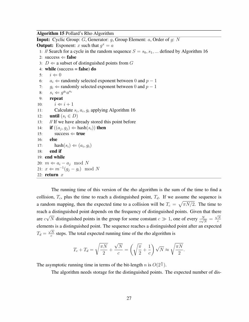
The running time of this version of the rho algorithm is the sum of the time to find acollision, Tc, plus the time to reach a distinguished point, Td. If we assume the sequence isa random mapping, then the expected time to a collision will be Tc =

√πN/2. The time to

reach a distinguished point depends on the frequency of distinguished points. Given that thereare c√N distinguished points in the group for some constant c � 1, one of every N

c√N

=√Nc

elements is a distinguished point. The sequence reaches a distinguished point after an expectedTd =

√Nc

steps. The total expected running time of the rho algorithm is

Tc + Td =

√πN

2+

√N

c=

(√π

2+

1

c

)√N ≈

√πN

2.

The asymptotic running time in terms of the bit-length n is O(2n2 ).

The algorithm needs storage for the distinguished points. The expected number of dis-

27

Algorithm 16 Pollard’s Rho - Random Sequence AlgorithmInput: Element: si, Exponents: ai, gi, such that si = aaiggi

Output: Element: si+1, Exponents: ai+1, gi+1, such that si+1 = aai+1ggi+1

1: // Given a partitioning of G into three equal-sized subsets S1, S2, S3

2: if si ∈ S1 then3: si+1 = asi4: ai+1 = ai + 1 mod N5: gi+1 = gi6: else if si ∈ S2 then7: si+1 = si

2

8: ai+1 = 2ai mod N9: gi+1 = 2gi mod N

10: else if si ∈ S3 then11: si+1 = gsi12: ai+1 = ai13: gi+1 = gi + 1 mod N14: end if15: return si+1, ai+1, gi+1

tinguished points will be the expected number of steps multiplied by the fraction of elementsthat are distinguished points,((√

π

2+

1

c

)√N

)(c√N

)= c

√π

2+ 1

For each distinguished point, we store a pair of n-bit exponents. Thus the total expected stor-age required by the algorithm is (c

√2π + 2)n bits. Because c is a constant, the total storage

requirement is O(n).

H. Pollard’s Kangaroo Algorithm

Another generic algorithm discovered by Pollard [22] is the kangaroo or lambda method.It has a runtime that differs from the Pollard’s Rho method by only a constant. It can also beused to find discrete logarithms when the exponent is known to lie in a smaller interval. Wepresent an improved version, due to van Oorschot and Weiner [27], that uses distinguishedpoints.

The kangaroo-method gets its name because it can be described with an analogy of twokangaroos hopping. If we imagine each element of the the cyclic group as being steps on a

28

Algorithm 17 Pollard’s Kangaroo AlgorithmInput: Cyclic Group: G, Generator: g, Group Element: a, Order of g: NOutput: Exponent: x such that gx = a

1: // Select a small sequence of possible step sizes2: S ⇐ (s0, s1, . . . , sk−1) where si = 2i and k such that the mean of the entries is

√N

3: R⇐ (r0, r1, . . . , rk−1) where ri = gsi

4: // Select a hash function to map a group element to a particular step size, si5: h(x)⇐ hash function mapping G into the interval [1..k]6: D ⇐ a subset of distinguished points from G7: // The “tame” kangaroo starts off half way through the cycle8: xt ⇐ g

N2

9: dt ⇐ 010: // The “wild” kangaroo starts off from a = gx

11: xw ⇐ a12: dw ⇐ 013: success⇐ false14: while (success = false) do15: // Step the tame kangaroo one hop16: i⇐ h(xt)17: xt ⇐ xtri18: dt ⇐ dt + si19: if xt ∈ D then20: // If we have already stored this point for a wild kangaroo21: if ((m,xi, di)⇐ hash(xt)) && (m = ’wild’) then22: x⇐ N

2+ dt − di

23: success⇐ true24: else25: hash(xt)⇐ (’tame’, xt, dt)26: end if27: end if28: // Step the wild kangaroo one hop29: i⇐ h(ww)30: xw ⇐ xwri31: dw ⇐ dw + si32: if xw ∈ D then33: // If we have already stored this point for a tame kangaroo34: if ((m,xi, di)⇐ hash(xw)) && (m = ’tame’) then35: x⇐ N

2+ di − dw

36: success⇐ true37: else38: hash(xw)⇐ (’wild’, xw, dw)39: end if40: end if41: end while42: return x

29

path, ordered by exponent, (g0, g1, g2, . . .), then each hop of the kangaroo is from one elementof the group to another. The distance of the hop, si, is selected from a small set of possible hopdistances S. The choice of si is based only on the current position, x, using a hash functionh(x) = i. This means that any kangaroo that lands on a particular element will always take thesame sequence of hops from then on.

The algorithm uses two kangaroos (sequences), one wild and one tame. The wild onestarts on element a = gx. Its starting position exponent, x is unknown; it is the discrete log-arithm that we are trying to find. We start the tame kangaroo at a known position, halfwaythrough the cycle, at g

N2 . We alternate stepping the wild and tame kangaroos. We keep track of

their respective positions, xw, xt, and their respective distances traveled, dw, dt.We want the wild kangaroo to land on the path of the tame kangaroo. Since we know the

exponent of the tame kangaroo, N2

+ dt, we can calculate the discrete logarithm by subtractingthe distance traveled by the wild kangaroo,

logg a = x ≡ N

2+ dt − dw mod N

As the two kangaroos jump, their paths will eventually converge.Anytime a kangaroo lands on a distinguished point, we store which kangaroo, the point,

and the distance traveled in a hash table. If the other kangaroo has already stored this point inthe hash table, then the paths have converged, and we can solve for the discrete logarithm. Theuse of distinguished points allows us to discover the convergence point quickly while reducingmemory accesses and storage requirements. Memory only needs to be read or written on thesmall percentage of steps that land on distinguished points.

To find the runtime and storage requirements, we follow the approximate analysis ofPollard [23]. We consider the algorithm as three stages:

1. The kangaroo in back must catch up with the starting point of the other kangaroo.

2. The back kangaroo must then land on the path of the other kangaroo.

3. The back kangaroo must continue until it reaches a distinguished point.

Throughout each stage, the back kangaroo could be either the wild or the tame kangaroo.At the start, the back kangaroo can be at most half a cycle behind and on average will be

a quarter of a cycle behind or N4

. The mean step size is m =√N2

, so the back kangaroo needsN4/√N2

=√N2

steps, on average, to catch up to the starting point of the front kangaroo. Giventhat the kangaroos alternate steps, the average running time of Stage 1 is

√N group operations.

30

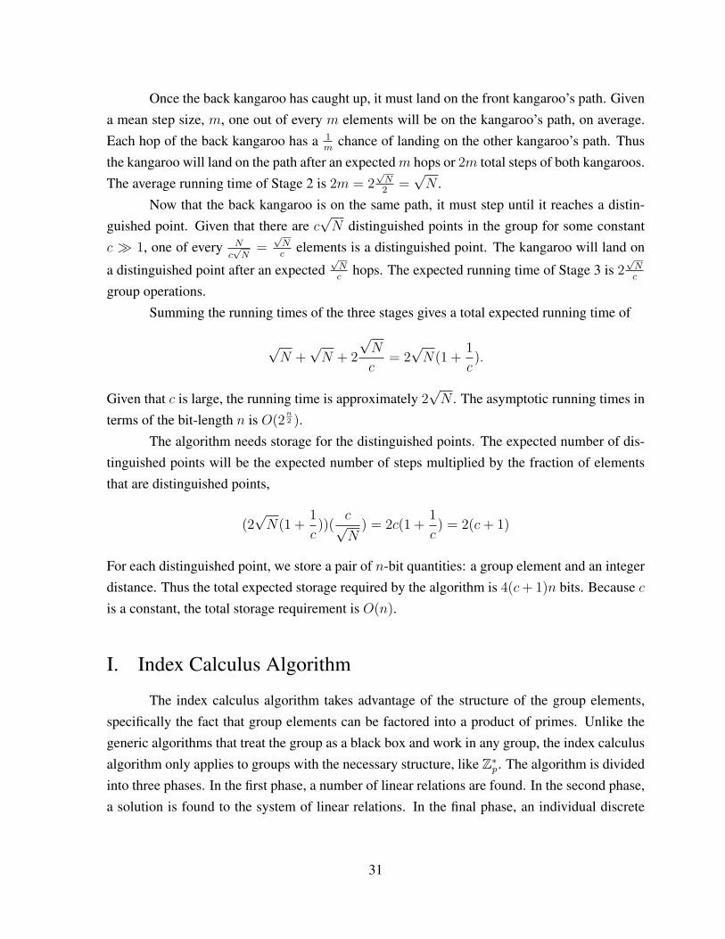
Once the back kangaroo has caught up, it must land on the front kangaroo’s path. Givena mean step size, m, one out of every m elements will be on the kangaroo’s path, on average.Each hop of the back kangaroo has a 1

mchance of landing on the other kangaroo’s path. Thus

the kangaroo will land on the path after an expectedm hops or 2m total steps of both kangaroos.The average running time of Stage 2 is 2m = 2

√N2

=√N .

Now that the back kangaroo is on the same path, it must step until it reaches a distin-guished point. Given that there are c

√N distinguished points in the group for some constant

c � 1, one of every Nc√N

=√Nc

elements is a distinguished point. The kangaroo will land on

a distinguished point after an expected√Nc

hops. The expected running time of Stage 3 is 2√Nc

group operations.Summing the running times of the three stages gives a total expected running time of

√N +

√N + 2

√N

c= 2√N(1 +

1

c).

Given that c is large, the running time is approximately 2√N . The asymptotic running times in

terms of the bit-length n is O(2n2 ).

The algorithm needs storage for the distinguished points. The expected number of dis-tinguished points will be the expected number of steps multiplied by the fraction of elementsthat are distinguished points,

(2√N(1 +

1

c))(

c√N

) = 2c(1 +1

c) = 2(c+ 1)

For each distinguished point, we store a pair of n-bit quantities: a group element and an integerdistance. Thus the total expected storage required by the algorithm is 4(c+ 1)n bits. Because cis a constant, the total storage requirement is O(n).

I. Index Calculus Algorithm

The index calculus algorithm takes advantage of the structure of the group elements,specifically the fact that group elements can be factored into a product of primes. Unlike thegeneric algorithms that treat the group as a black box and work in any group, the index calculusalgorithm only applies to groups with the necessary structure, like Z∗p . The algorithm is dividedinto three phases. In the first phase, a number of linear relations are found. In the second phase,a solution is found to the system of linear relations. In the final phase, an individual discrete

31

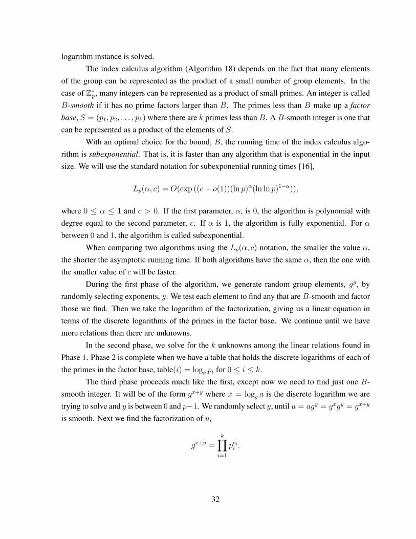
logarithm instance is solved.The index calculus algorithm (Algorithm 18) depends on the fact that many elements

of the group can be represented as the product of a small number of group elements. In thecase of Z∗p , many integers can be represented as a product of small primes. An integer is calledB-smooth if it has no prime factors larger than B. The primes less than B make up a factor

base, S = (p1, p2, . . . , pk) where there are k primes less than B. A B-smooth integer is one thatcan be represented as a product of the elements of S.

With an optimal choice for the bound, B, the running time of the index calculus algo-rithm is subexponential. That is, it is faster than any algorithm that is exponential in the inputsize. We will use the standard notation for subexponential running times [16],

Lp(α, c) = O(exp ((c+ o(1))(ln p)α(ln ln p)1−α)),

where 0 ≤ α ≤ 1 and c > 0. If the first parameter, α, is 0, the algorithm is polynomial withdegree equal to the second parameter, c. If α is 1, the algorithm is fully exponential. For αbetween 0 and 1, the algorithm is called subexponential.

When comparing two algorithms using the Lp(α, c) notation, the smaller the value α,the shorter the asymptotic running time. If both algorithms have the same α, then the one withthe smaller value of c will be faster.

During the first phase of the algorithm, we generate random group elements, gy, byrandomly selecting exponents, y. We test each element to find any that are B-smooth and factorthose we find. Then we take the logarithm of the factorization, giving us a linear equation interms of the discrete logarithms of the primes in the factor base. We continue until we havemore relations than there are unknowns.

In the second phase, we solve for the k unknowns among the linear relations found inPhase 1. Phase 2 is complete when we have a table that holds the discrete logarithms of each ofthe primes in the factor base, table(i) = logg pi for 0 ≤ i ≤ k.

The third phase proceeds much like the first, except now we need to find just one B-smooth integer. It will be of the form gx+y where x = logg a is the discrete logarithm we aretrying to solve and y is between 0 and p−1. We randomly select y, until u = agy = gxgy = gx+y

is smooth. Next we find the factorization of u,

gx+y =k∏i=1

pcii .

32

Algorithm 18 Index Calculus AlgorithmInput: Prime: p, Generator of Z∗p: g, Element of Z∗p: aOutput: Exponent: x satisfying gx ≡ a mod p, where 0 ≤ x < p− 1.

1: // Setup: Select a factor base2: B ⇐ a bound for the largest prime in the factor base, S3: S ⇐ (p1, p2, . . . , pk) where S contains all primes, pi < B4: // Phase 1: Find linear relations of the factor base5: // Find a few more relations than the size of the factor base to ensure a unique solution6: for j = 0 to k + c do7: repeat8: y ⇐ randomly selected exponent between 0 and p− 19: u⇐ gy mod p

10: until (u is B-smooth)11: // Find the factorization of u12: u =

∏1≤i≤k

pcii

13: // Take logarithms and store the linear relation14: y =

∑1≤i≤k

ci logg pi (mod p− 1)

15: end for16: // Phase 2: Solve system of linear relations17: Given the k + c relations from Phase 1, solve for the k unknown discrete logarithms of the

factor base.18: Store the logarithms, such that table(i) = logg pi, 1 ≤ i ≤ k19: // Phase 3: Solve for the individual discrete logarithm20: repeat21: y ⇐ randomly selected exponent between 0 and p− 122: u⇐ agy mod p23: until (u is B-smooth)24: // Find the factorization of u25: u =

∏1≤i≤k

pcii

26: // Take logarithms of both sides27: x+ y =

∑1≤i≤k


28: x⇐∑

1≤i≤k

ci table(i)− y (mod p− 1)

29: return x

33

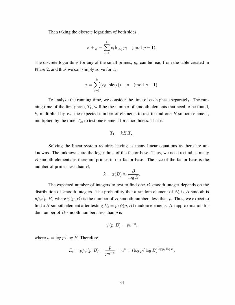
Then taking the discrete logarithm of both sides,

x+ y =k∑i=1

ci logg pi (mod p− 1).

The discrete logarithms for any of the small primes, pi, can be read from the table created inPhase 2, and thus we can simply solve for x,

x =k∑i=1

(citable(i))− y (mod p− 1).

To analyze the running time, we consider the time of each phase separately. The run-ning time of the first phase, T1, will be the number of smooth elements that need to be found,k, multiplied by Es, the expected number of elements to test to find one B-smooth element,multiplied by the time, Ts, to test one element for smoothness. That is

T1 = kEsTs.

Solving the linear system requires having as many linear equations as there are un-knowns. The unknowns are the logarithms of the factor base. Thus, we need to find as manyB-smooth elements as there are primes in our factor base. The size of the factor base is thenumber of primes less than B,

k = π(B) ≈ B

logB.

The expected number of integers to test to find one B-smooth integer depends on thedistribution of smooth integers. The probability that a random element of Z∗p is B-smooth isp/ψ(p,B) where ψ(p,B) is the number of B-smooth numbers less than p. Thus, we expect tofind a B-smooth element after testing Es = p/ψ(p,B) random elements. An approximation forthe number of B-smooth numbers less than p is

ψ(p,B) = pu−u,

where u = log p/ logB. Therefore,

Es = p/ψ(p,B) =p

pu−u= uu = (log p/ logB)log p/ logB.

34

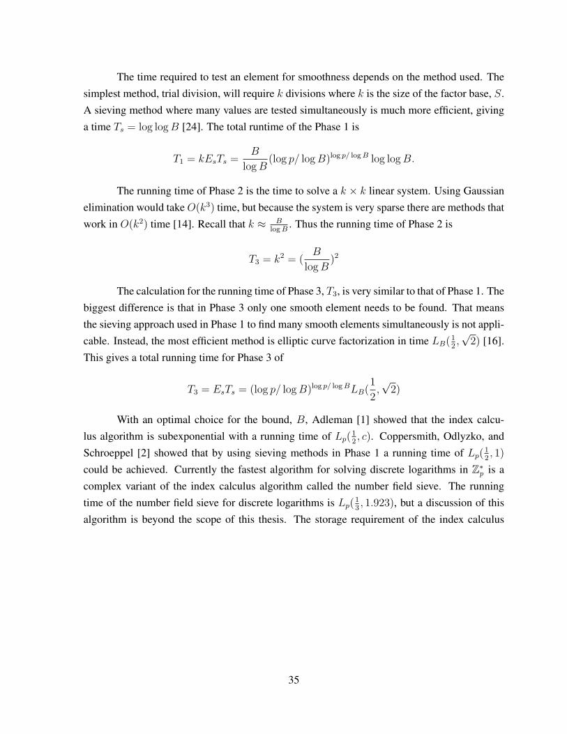
The time required to test an element for smoothness depends on the method used. Thesimplest method, trial division, will require k divisions where k is the size of the factor base, S.A sieving method where many values are tested simultaneously is much more efficient, givinga time Ts = log logB [24]. The total runtime of the Phase 1 is

T1 = kEsTs =B

logB(log p/ logB)log p/ logB log logB.

The running time of Phase 2 is the time to solve a k × k linear system. Using Gaussianelimination would takeO(k3) time, but because the system is very sparse there are methods thatwork in O(k2) time [14]. Recall that k ≈ B

logB. Thus the running time of Phase 2 is

T3 = k2 = (B

logB)2

The calculation for the running time of Phase 3, T3, is very similar to that of Phase 1. Thebiggest difference is that in Phase 3 only one smooth element needs to be found. That meansthe sieving approach used in Phase 1 to find many smooth elements simultaneously is not appli-cable. Instead, the most efficient method is elliptic curve factorization in time LB(1

2,√

2) [16].This gives a total running time for Phase 3 of

T3 = EsTs = (log p/ logB)log p/ logBLB(1

2,√

2)

With an optimal choice for the bound, B, Adleman [1] showed that the index calcu-lus algorithm is subexponential with a running time of Lp(1

2, c). Coppersmith, Odlyzko, and

Schroeppel [2] showed that by using sieving methods in Phase 1 a running time of Lp(12, 1)

could be achieved. Currently the fastest algorithm for solving discrete logarithms in Z∗p is acomplex variant of the index calculus algorithm called the number field sieve. The runningtime of the number field sieve for discrete logarithms is Lp(1

3, 1.923), but a discussion of this

algorithm is beyond the scope of this thesis. The storage requirement of the index calculus

35

algorithm is the space needed to represent the system of linear equations. Although the systembeing solved is k × k, the system is very sparse and the zero entries need not be stored. Eachequation will have fewer than logB non-zero entries of size n. So the asymptotic size of theindex calculus algorithm is

nB

logBlogB = nB.

To achieve the optimal running time for the index calculus algorithm the choice ofB is Lp(12, 1

2).

J. Summary

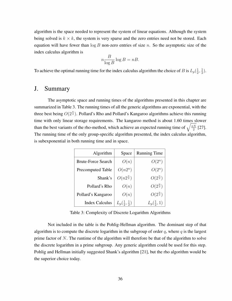
The asymptotic space and running times of the algorithms presented in this chapter aresummarized in Table 3. The running times of all the generic algorithms are exponential, with thethree best being O(2

n2 ). Pollard’s Rho and Pollard’s Kangaroo algorithms achieve this running

time with only linear storage requirements. The kangaroo method is about 1.60 times slowerthan the best variants of the rho-method, which achieve an expected running time of

√πN2

[27].The running time of the only group-specific algorithm presented, the index calculus algorithm,is subexponential in both running time and in space.

Algorithm Space Running Time

Brute-Force Search O(n) O(2n)

Precomputed Table O(n2n) O(2n)

Shank’s O(n2n2 ) O(2

n2 )

Pollard’s Rho O(n) O(2n2 )

Pollard’s Kangaroo O(n) O(2n2 )

Index Calculus Lp(12, 1

2) Lp(

12, 1)

Table 3: Complexity of Discrete Logarithm Algorithms

Not included in the table is the Pohlig-Hellman algorithm. The dominant step of thatalgorithm is to compute the discrete logarithm in the subgroup of order q, where q is the largestprime factor of N . The runtime of the algorithm will therefore be that of the algorithm to solvethe discrete logarithm in a prime subgroup. Any generic algorithm could be used for this step.Pohlig and Hellman initially suggested Shank’s algorithm [21], but the rho algorithm would bethe superior choice today.

36

IV. Complexity of Discrete Logarithms over Fixed Groups

In this chapter, we examine the complexity of discrete logarithms over fixed groups. Inparticular, we introduce the para-discrete logarithm problem, a variant of the discrete logarithmproblem that more closely models cryptologic applications over fixed groups. Next, we discusshow to model an adversary with access to a group-specific precomputation. Then we re-examineeach algorithm from the previous chapter as a para-discrete logarithm solver. We summarizethe analysis with a chart showing the run times and precomputation sizes for each algorithm.We then apply our analysis of generic algorithms to place an upper bound on the complexity ofthe generalized para-discrete logarithm problem. Finally, we use our analysis of index calculusalgorithms to place an upper bound on the para-discrete logarithm problem.

A. The Para-Discrete Logarithm Problem

Complexity theoretic models are useful for evaluating the security of real world crypto-graphic applications. However, a model can also provide a false sense of security if it oversim-plifies the implementation details or makes bad assumptions about the capabilities of the adver-sary. To illustrate this point, imagine a protocol that implements ElGamal public key encryption.This hypothetical protocol requires a user to prove they know their private key by respondingwith the plaintext after receiving an encrypted random number as a challenge. This allows anadversary to mount a chosen ciphertext attack. Consider an adversary who intercepts a cipher-text, (c1 = gb, c2 = gabm), encrypted with user A’s public key, ga, and wants to read the secretmessage, m. The adversary selects a random, r, and sends (c′1 = c1 = gb, c′2 = c2r = gabmr) tothe userA as a random number challenge. UserAwill decrypt and return the seemingly randommessage, m′ = mr. From m′, the attacker easily solves for m by multiplying by r−1, givingm = mrr−1. Thus, if ElGamal is used within a flawed protocol, the difficulty of the discretelogarithm problem is irrelevant. A security model must consider the protocol as a whole andnot just the underlying cryptography.

37

The use of fixed groups in security protocols inspires the question: Do our existingmodels sufficiently capture these applications? In the DLP and GDLP, the group and generatorare inputs to the problem along with a particular instance to solve. Yet in a fixed group imple-mentation, every instance takes place over the same small set of groups. Does this provide anadvantage to an adversary? We propose a new complexity problem that more closely modelsthese fixed group protocols, the para-discrete logarithm problem.

Definition 19 The Para-Discrete Logarithm Problem (PDLP)

Setup: Let p = p2, p3, p4, . . . be an infinite sequence of primes, where pi is a prime of bit-length, i. Let g = g2, g3, g4, . . . be an infinite sequence of integers, where 0 < gi < piand gi generates Z∗pi

.

Input: Security Parameter: 1n, Group Element: a ∈ Z∗pn, where pn ∈ p.

Output: Exponent: x satisfying gnx ≡ a mod pn, where gn ∈ g

Unlike in the standard discrete logarithm problem, the group and generator are not inputsto the para-discrete logarithm problem. Instead, there is just a security parameter, 1n, thatspecifies the bit-length of the prime modulus. The prime modulus, pn, comes from an infinitesequence of primes, with exactly one prime for a given bit-length. We contend this problemis a better computational model for discrete logarithms over fixed groups, because for a givensecurity parameter there is a single defined group.

Just as the discrete logarithm problem can be generalized from Z∗p to any cyclic groupG, we can generalize the para-discrete logarithm problem.

Definition 20 The Generalized Para-Discrete Logarithm Problem (GPDLP)

Setup: Let G = G1, G2, G3, . . . be an infinite sequence of groups, where Gi is a cyclic groupof order Ni, such that 2i−1 < Ni ≤ 2i. Let g = g1, g2, g3, . . . be an infinite sequence ofgroup elements, where gi ∈ Gi and gi generates Gi.

Input: Security Parameter: 1n, Group Element: a ∈ Gn, where Gn ∈ G.

Output: Exponent: x satisfying gnx = a, where gn ∈ g

Just as in the PDLP, the group is not an input to the GPDLP problem. Instead, the groupis determined by the security parameter 1n. For a given n, the group is fixed to Gn where Gn isan element of an infinite sequence of groups G1, G2, ....

38

B. The Para-Discrete Logarithm Problem with an Advice String

By removing the group as an input to the problem, the PDLP more closely models fixedgroup applications. In applications where groups are generated on the fly and used once, theadversary gains no advantage through a precomputation; the precomputation can only be usedonce. In contrast, with fixed groups a precomputation can provide the adversary an advantagefor all instances over the life of the cryptographic application.

We model this precomputation as an advice string. In computational complexity theoryan advice string is an extra input to a computational problem that depends only on the length ofthe input. By the definition of the PDLP, the group is fixed for a given input length. This allowsus to consider a group-specific computation as producing an advice string for the PDLP. (In thestandard DLP setting, the precomputation could not be considered an advice string because it isdependent on an input to the problem, the specific group.)

We assert that a conservative approach to evaluating the security of a protocol is to con-sider an attack where the adversary has access to a precomputation based only on the protocolstandard. In the case of a protocol with fixed groups, we should consider an adversary withaccess to a group-specific precomputation. Using the advice-string formalism allows us to bet-ter consider the difficulty of solving discrete logarithms once a group-specific precomputationhas been completed. We can consider the time and space complexity of solving the instanceseparately from the time to create the precomputation.

C. Para-Discrete Logarithm Algorithms

In this section, we re-examine each algorithm from the previous chapter as a para-discrete logarithm solver. We want to analyze the complexity of the PDLP with an advicestring. To assist this, we explicitly divide each algorithm into two sub-algorithms: the advice-generator (precomputation phase) and the instance-solver (search phase). The advice-generatorperforms a precomputation based only on the group and generator, not the specific probleminstance. That allows us to treat the precomputation’s output as an advice string for the PDLP.The instance-solver searches for the solution of a specific problem instance making use of theadvice string. For each algorithm, we determine the asymptotic runtime of both phases and thesize of the advice string.

39

1. Brute-Force Search and Precomputed Table Algorithms

We begin our re-examination, with the two simplest algorithms. In the brute-forcesearch, there is no precomputation done. If we try to modify the brute-force search to havea precomputation, we end up with the precomputed table algorithm. The precomputed tablealgorithm very naturally divides into the two algorithms we are looking for. In the advice-generator algorithm, the table of all logarithms is built. In the instance-solver algorithm a singlelookup into the table returns the discrete logarithm.

Algorithm 21 Precomputed Table: Advice GeneratorInput: Cyclic Group: G, Generator: gOutput: Advice string: hash such that hash[gx] = x for 0 ≤ x < N

1: b⇐ 12: for x = 0 to N − 1 do3: hash[b]⇐ x4: b⇐ b× g5: end for6: return hash

Algorithm 22 Precomputed Table: Instance SolverInput: Group Element: a, Advice string: hashOutput: Exponent: x such that gx = a

1: x⇐ hash[a]2: return x

The advice-generator will require N group multiplications to preform the precomputa-tion. The asymptotic running time of the advice-generator is O(2n). The size of the advicestring (the precomputed hash table containing N exponents) is exponential in n, O(n2n). Afterthe precomputation, the instance solver requires a single table lookup to solve an individualdiscrete log.

2. Shank’s Algorithm

The hash table built in Shank’s algorithm is independent of a particular discrete loga-rithm instance, so the hash table can act as the advice string. That is, the advice-generator buildsthe hash table. The instance-solver then giant-steps from the input a until it reaches an elementwith a precomputed discrete logarithm in the hash table.

40

Algorithm 23 Shank’s Algorithm: Advice GeneratorInput: Cyclic Group: G, Generator: g, Number of exponents to precompute: XOutput: Advice string: hash such that hash[gi] = i for 0 ≤ i < X

1: b⇐ 12: for i = 0 to X − 1 do3: hash[b]⇐ i4: b⇐ b× g5: end for6: return hash

Algorithm 24 Shank’s Algorithm: Instance SolverInput: Group Element: a, Advice string: hash, Number of precomputed logarithms: XOutput: Exponent: x such that gx = a

1: b⇐ a2: y ⇐ 03: h⇐ hash[b]4: while gh 6= b do5: b⇐ b× gX6: y ⇐ y + 17: h⇐ hash[b]8: end while9: x⇐ h− yX mod N

10: return x

Now we consider the runtime of each algorithm. For general X , the advice-generatortakes X group operations to generate an advice string with X entries of size n-bits, resulting inan advice string of O(nX). The instance-solver takes, on average, N

2Xoperations. For X = 2

n2 ,

both the advice generator and instance-solver take 2n2 group operations. Therefore, the runtime

complexity of both algorithms is O(2n2 ) with an advice string of O(n2

n2 ).

The best choice ofX varies depending on the particular trade-offs of a given application.A smaller choice for X means a quicker precomputation and a smaller advice string, but atthe expense of a longer runtime for the instance solver. Likewise, a larger X means quickerinstance solving, but at the expense of a larger advice-string and a longer runtime for the advicegenerator. Note that for X = 1 we have essentially the brute-force search, and for X = N wehave the precomputed table algorithm.

Given a desired number, k, of instances to solve in a particular group, we can select anXto minimize overall computation time. The total computation time is that of one precomputation

41

plus k instance computations,

f(X) = X + kN

2X.

To minimize f(X), we find the positive zero of the derivative,

d

dXf(X) = 1− kN

2X2= 0,

kN

2X2= 1,

X2 =kN

2,

X =

√kN

2.

Therefore, the best choice ofX to minimize computation time when solving k instances is√

kN2

or, in terms of the bit-length, n, X =√k2

n−12 . This gives a total computation time of

√2kN

and an average time per solution of√

2kNk

=√

2Nk

.

3. Pollard’s Rho Algorithm

As we examine Pollard’s Rho algorithm, we see that it does not fit the two-phase pattern.The algorithm only requires a small amount of storage while running and does not make useof a precomputation. The random sequence depends on a particular instance, a = gx, we aretrying to solve. It it not immediately clear how a instance-independent precomputation couldassist this algorithm. Using our terminology there is only an instance-solver algorithm and ituses no advice string.

However, [13] analyzes how work can be saved from each instance of the rho algorithm,speeding the solution of subsequent instances over the same group. They note that the tableof distinguished points stored during computation of one logarithm becomes a table of knownlogarithms once that instance has a solution. Those distinguished points can be saved andused to assist the next instance and so on. The saved distinguished points are effectively aprecomputation for solving the next instance.

This idea can be extended to create a useful advice string, a database of logarithms ofdistinguished points. The advice generator selects random exponents, i, to create random ele-ments, gi, and stores the discrete logarithm each time a distinguished point is found. Additional

42

distinguished points are found until the desired advice size has been reached. Let d be the num-ber of distinguished point logarithms we precompute. In one extreme, where d = 0, we have thestandard rho algorithm. At the other extreme, where d equals the total number of distinguishedpoints in the group, we completely remove the benefit of finding cycles in the random sequence;the first time we reach a distinguished point, we can solve the logarithm. This extreme is clearlyinferior to Shank’s algorithm where precomputing each logarithm requires only a single groupoperation.

Algorithm 25 Pollard’s Rho Algorithm: Advice GeneratorInput: Cyclic Group: G, Generator: g, Order of g: N , Number of logarithms of distinguished

points to precompute: dOutput: Advice string: hash such that hash[aaiggi ] = (ai, gi) for some aaiggi ∈ D

1: D ⇐ a subset of distinguished points from G2: // Randomly chose exponents and store logarithms of d distinguished points3: for j = 1 to d do4: repeat5: i⇐ randomly selected exponent between 0 and p− 16: si ⇐ gi

7: until (si ∈ D)8: hash(si)⇐ (0, i)9: end for

10: return hash

Kuhn and Struik [13] show that computing a total of X logarithms in the same grouptakes time

√2NX and that the X + 1 logarithm can be computed in time

√N/2X for X <<

N1/4.We design our advice generator so that it creates the number of distinguished points, d,

equivalent to having solved X logarithms. Because the results of Kuhn and Struik are limitedto X << N1/4, we let X = N1/5. The advice generator will take time

Tadvice =√

2NX =√

2N(N1/5) =√

2N6/5 =√

2N3/5.

The instance solver will take time

Tinstance =√N/2X =

√N/2N1/5 =

√N4/5/2 =

1√2N2/5.

The size of advice depends on θ, the proportion of elements that are distinguished points. Forthe time estimate of the instance solver to be accurate, it must reach many distinguished points.

43

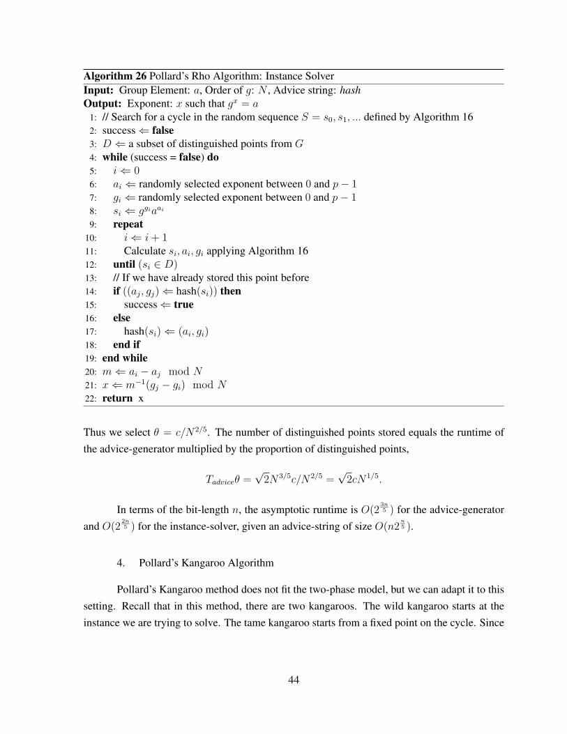
Algorithm 26 Pollard’s Rho Algorithm: Instance SolverInput: Group Element: a, Order of g: N , Advice string: hashOutput: Exponent: x such that gx = a

1: // Search for a cycle in the random sequence S = s0, s1, ... defined by Algorithm 162: success⇐ false3: D ⇐ a subset of distinguished points from G4: while (success = false) do5: i⇐ 06: ai ⇐ randomly selected exponent between 0 and p− 17: gi ⇐ randomly selected exponent between 0 and p− 18: si ⇐ ggiaai

9: repeat10: i⇐ i+ 111: Calculate si, ai, gi applying Algorithm 1612: until (si ∈ D)13: // If we have already stored this point before14: if ((aj, gj)⇐ hash(si)) then15: success⇐ true16: else17: hash(si)⇐ (ai, gi)18: end if19: end while20: m⇐ ai − aj mod N21: x⇐ m−1(gj − gi) mod N22: return x

Thus we select θ = c/N2/5. The number of distinguished points stored equals the runtime ofthe advice-generator multiplied by the proportion of distinguished points,

Tadviceθ =√

2N3/5c/N2/5 =√

2cN1/5.

In terms of the bit-length n, the asymptotic runtime is O(23n5 ) for the advice-generator

and O(22n5 ) for the instance-solver, given an advice-string of size O(n2

n5 ).

4. Pollard’s Kangaroo Algorithm

Pollard’s Kangaroo method does not fit the two-phase model, but we can adapt it to thissetting. Recall that in this method, there are two kangaroos. The wild kangaroo starts at theinstance we are trying to solve. The tame kangaroo starts from a fixed point on the cycle. Since

44

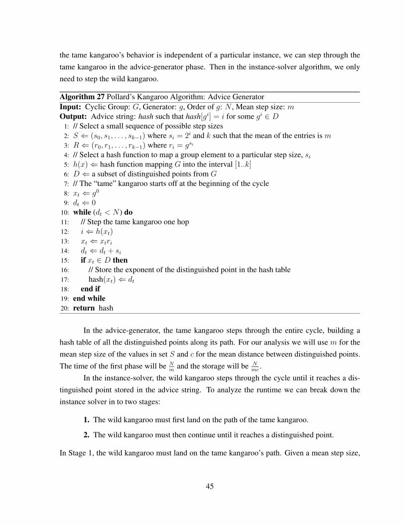
the tame kangaroo’s behavior is independent of a particular instance, we can step through thetame kangaroo in the advice-generator phase. Then in the instance-solver algorithm, we onlyneed to step the wild kangaroo.

Algorithm 27 Pollard’s Kangaroo Algorithm: Advice GeneratorInput: Cyclic Group: G, Generator: g, Order of g: N , Mean step size: mOutput: Advice string: hash such that hash[gi] = i for some gi ∈ D

1: // Select a small sequence of possible step sizes2: S ⇐ (s0, s1, . . . , sk−1) where si = 2i and k such that the mean of the entries is m3: R⇐ (r0, r1, . . . , rk−1) where ri = gsi

4: // Select a hash function to map a group element to a particular step size, si5: h(x)⇐ hash function mapping G into the interval [1..k]6: D ⇐ a subset of distinguished points from G7: // The “tame” kangaroo starts off at the beginning of the cycle8: xt ⇐ g0

9: dt ⇐ 010: while (dt < N ) do11: // Step the tame kangaroo one hop12: i⇐ h(xt)13: xt ⇐ xtri14: dt ⇐ dt + si15: if xt ∈ D then16: // Store the exponent of the distinguished point in the hash table17: hash(xt)⇐ dt18: end if19: end while20: return hash

In the advice-generator, the tame kangaroo steps through the entire cycle, building ahash table of all the distinguished points along its path. For our analysis we will use m for themean step size of the values in set S and c for the mean distance between distinguished points.The time of the first phase will be N

mand the storage will be N

mc.

In the instance-solver, the wild kangaroo steps through the cycle until it reaches a dis-tinguished point stored in the advice string. To analyze the runtime we can break down theinstance solver in to two stages:

1. The wild kangaroo must first land on the path of the tame kangaroo.

2. The wild kangaroo must then continue until it reaches a distinguished point.

In Stage 1, the wild kangaroo must land on the tame kangaroo’s path. Given a mean step size,

45

Algorithm 28 Pollard’s Kangaroo Algorithm: Instance SolverInput: Group Element: a, Order of g: N , Advice string: hashOutput: Exponent: x such that gx = a

1: // Use the same set S as in the advice-generator2: S ⇐ (s0, s1, . . . , sk−1) where si = 2i and k such that the mean of the entries is m3: R⇐ (r0, r1, . . . , rk−1) where ri = gsi

4: // Use the same hash function as in the advice-generator5: h(x)⇐ hash function mapping G into the interval [1..k]6: D ⇐ a subset of distinguished points from G7: // The “wild” kangaroo starts off from a = gx

8: xw ⇐ a9: dw ⇐ 0

10: success⇐ false11: while (success = false) do12: // Step the wild kangaroo one hop13: i⇐ h(ww)14: xw ⇐ xwri15: dw ⇐ dw + si16: if xw ∈ D then17: // If we have already stored this point for a tame kangaroo18: if (di ⇐ hash(xw)) then19: x⇐ di − dw mod N20: success⇐ true21: end if22: end if23: end while24: return x

m, each hop of the wild kangaroo has a 1m

chance of landing on the tame kangaroo’s path. Thusthe kangaroo will land on the path after an expected m hops.

In Stage 2, the wild kangaroo is on the path of the tame kangaroo and must reach a dis-tinguished point. Given that one of every c elements is a distinguished point, the wild kangaroowill land on a distinguished point after an expected c hops.

Combining the times from both stages gives a total runtime of m + c for the instance-solver. If we select c = m, the runtime becomes 2m and the size of the advice string is N

m2 .We can perform a trade-off between the runtime and the size of the advice string by varying m.One interesting trade-off is to balance the size of the advice string with the runtime,

N

m2= 2m.

46

Solving for m,

m3 =N

2,

m =3

√N

2.

This gives us a advice size and instance-solver time of 2m = 3√

4N . The advice-generator timeis

N

m=

3√

2N3√N

=3√

2N23 .

In terms of n, the bit-length of N , the instance-solver runs in O(2n3 ) time with an O(2

n3 ) size

advice string. The advice-generator runs in O(22n3 ) time.

5. Index Calculus Algorithm

The index calculus algorithm needs essentially no changes to match our desired two al-gorithm pattern. Phases 1 & 2 already use only the group description to create a precomputationresult. Combined, the first two phases become the advice-generator. The table of logarithmsof the factor base becomes the advice string, and final phase becomes our instance-solver algo-rithm.

The runtime of the advice generator will be the runtime of Phase 1 and Phase 2 of thestandard index calculus algorithm,

tadvice = T1 + T2 =B

logB(log p/ logB)log p/ logB log logB + (

B

logB)2.

The runtime of the instance generator is that of Phase 3,

tinstance = T3 = (log p/ logB)log p/ logBLB(1

2,√

2).

The size of the advice string will be the size of the table of logarithms of the factor base,

nk = nB

logB.

Looking at the structure of the algorithm, there is clearly a large imbalance betweenthe runtime of the advice-generator and that of the instance-solver. The instance solver has tofind only a single B-smooth integer, while the advice-generator must find k + c ≈ k B-smooth

47

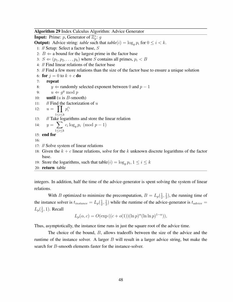
Algorithm 29 Index Calculus Algorithm: Advice GeneratorInput: Prime: p, Generator of Z∗p: gOutput: Advice string: table such that table(i) = logg pi for 0 ≤ i < k.

1: // Setup: Select a factor base, S2: B ⇐ a bound for the largest prime in the factor base3: S ⇐ (p1, p2, . . . , pk) where S contains all primes, pi < B4: // Find linear relations of the factor base5: // Find a few more relations than the size of the factor base to ensure a unique solution6: for j = 0 to k + c do7: repeat8: y ⇐ randomly selected exponent between 0 and p− 19: u⇐ gy mod p

10: until (u is B-smooth)11: // Find the factorization of u12: u =

∏1≤i≤k

pcii

13: // Take logarithms and store the linear relation14: y =

∑1≤i≤k


15: end for16:17: // Solve system of linear relations18: Given the k + c linear relations, solve for the k unknown discrete logarithms of the factor

base.19: Store the logarithms, such that table(i) = logg pi, 1 ≤ i ≤ k20: return table

integers. In addition, half the time of the advice-generator is spent solving the system of linearrelations.

With B optimized to minimize the precomputation, B = Lp(12, 1

2), the running time of

the instance solver is tinstance = Lp(12, 1

2) while the runtime of the advice-generator is tadvice =

Lp(12, 1). Recall

Lp(α, c) = O(exp ((c+ o(1))(ln p)α(ln ln p)1−α)),

Thus, asymptotically, the instance time runs in just the square root of the advice time.The choice of the bound, B, allows tradeoffs between the size of the advice and the

runtime of the instance solver. A larger B will result in a larger advice string, but make thesearch for B-smooth elements faster for the instance-solver.

48

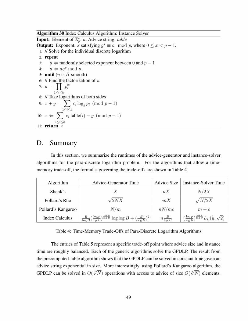
Algorithm 30 Index Calculus Algorithm: Instance SolverInput: Element of Z∗p: a, Advice string: tableOutput: Exponent: x satisfying gx ≡ a mod p, where 0 ≤ x < p− 1.

1: // Solve for the individual discrete logarithm2: repeat3: y ⇐ randomly selected exponent between 0 and p− 14: u⇐ agy mod p5: until (u is B-smooth)6: // Find the factorization of u7: u =

∏1≤i≤k

pcii

8: // Take logarithms of both sides9: x+ y =

∑1≤i≤k


10: x⇐∑

1≤i≤k

ci table(i)− y (mod p− 1)

11: return x

D. Summary

In this section, we summarize the runtimes of the advice-generator and instance-solveralgorithms for the para-discrete logarithm problem. For the algorithms that allow a time-memory trade-off, the formulas governing the trade-offs are shown in Table 4.

Algorithm Advice-Generator Time Advice Size Instance-Solver Time

Shank’s X nX N/2X

Pollard’s Rho√

2NX cnX√N/2X

Pollard’s Kangaroo N/m nN/mc m+ c

Index Calculus BlogB

( log plogB

)log plog B log logB + ( B

logB)2 n B

logB( log p

logB)

log plog BLB(1

2,√

2)

Table 4: Time-Memory Trade-Offs of Para-Discrete Logarithm Algorithms

The entries of Table 5 represent a specific trade-off point where advice size and instancetime are roughly balanced. Each of the generic algorithms solve the GPDLP. The result fromthe precomputed-table algorithm shows that the GPDLP can be solved in constant time given anadvice string exponential in size. More interestingly, using Pollard’s Kangaroo algorithm, theGPDLP can be solved in O( 3

√N) operations with access to advice of size O( 3

√N) elements.

49

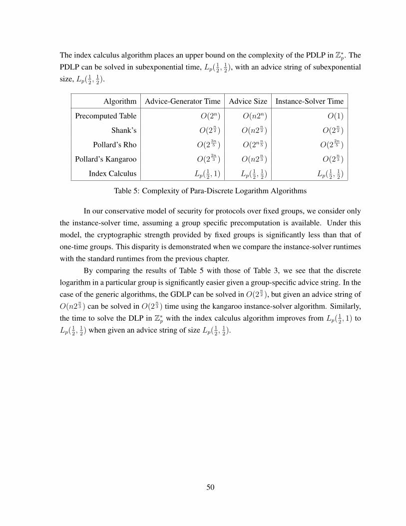
The index calculus algorithm places an upper bound on the complexity of the PDLP in Z∗p . ThePDLP can be solved in subexponential time, Lp(1

2, 1

2), with an advice string of subexponential

size, Lp(12, 1

2).

Algorithm Advice-Generator Time Advice Size Instance-Solver Time

Precomputed Table O(2n) O(n2n) O(1)

Shank’s O(2n2 ) O(n2

n2 ) O(2

n2 )

Pollard’s Rho O(23n5 ) O(2n

n5 ) O(2

2n5 )

Pollard’s Kangaroo O(22n3 ) O(n2

n3 ) O(2

n3 )

Index Calculus Lp(12, 1) Lp(

12, 1

2) Lp(

12, 1

2)

Table 5: Complexity of Para-Discrete Logarithm Algorithms

In our conservative model of security for protocols over fixed groups, we consider onlythe instance-solver time, assuming a group specific precomputation is available. Under thismodel, the cryptographic strength provided by fixed groups is significantly less than that ofone-time groups. This disparity is demonstrated when we compare the instance-solver runtimeswith the standard runtimes from the previous chapter.

By comparing the results of Table 5 with those of Table 3, we see that the discretelogarithm in a particular group is significantly easier given a group-specific advice string. In thecase of the generic algorithms, the GDLP can be solved in O(2

n2 ), but given an advice string of

O(n2n3 ) can be solved in O(2

n3 ) time using the kangaroo instance-solver algorithm. Similarly,

the time to solve the DLP in Z∗p with the index calculus algorithm improves from Lp(12, 1) to

Lp(12, 1

2) when given an advice string of size Lp(1

2, 1

2).

50

LIST OF REFERENCES

[1] L. Adleman. “A subexponential algorithm for the discrete logarithm problem with appli-cations to cryptography.” In 20th Annual Symposium on Foundations of Computer Sci-ence(SFCS 1979), pages 55–60. IEEE Computer Society, Los Alamitos, CA, USA, 1979.ISSN 0272-5428.

[2] D. Coppersmith, A. M. Odlyzko, and R. Schroeppel. “Discrete Logarithms in GF(p),”Algorithmica, 1(1):1–15, 1986.

[3] W. Diffie and M. Hellman. “New directions in cryptography,” IEEE Transactions onInformation Theory, 22(6):644–654, 1976.

[4] T. El Gamal. “A public key cryptosystem and a signature scheme based on discrete loga-rithms.” In Proceedings of Advances in Cryptology (CRYPTO 84), number 196 in LectureNotes in Computer Science, pages 10–18. Springer, New York, NY, 1985.

[5] M. Friedl, N. Provos, and W. Simpson. “Diffie-Hellman Group Exchange for the SecureShell (SSH) Transport Layer Protocol.” RFC 4419 (Proposed Standard), March 2006.Accessed March 25, 2010. http://www.ietf.org/rfc/rfc4419.txt, IETF.

[6] S. Goldwasser and S. Micali. “Probabilistic encryption,” Journal of Computer and SystemsSciences, 28(2):270–299, 1984.

[7] S. Goldwasser, S. Micali, and R. Rivest. “A Digital Signature Scheme Secure AgainstAdaptive Chosen-Message Attacks.”, SIAM Journal on Computing, 17:281–308, 1988.

[8] D. M. Gordon. “A survey of fast exponentiation methods,” Journal of algorithms, 27(1):129–146, 1998.

[9] D. M. Gordon and K. S. McCurley. “Massively parallel computation of discrete loga-rithms.” In Advances in Cryptology CRYPTO 92, Lecture Notes in Computer Science,page 312. Springer, New York, NY, 1993.

[10] D. Harkins and D. Carrel. “The Internet Key Exchange (IKE).” RFC 2409 (ProposedStandard), November 1998. Accessed March 25, 2010. http://www.ietf.org/rfc/rfc2409.txt, IETF. Obsoleted by RFC 4306, updated by RFC 4109.

51

http://www.ietf.org/rfc/rfc4419.txt



[11] A. Hildebrand and G. Tenenbaum. “On Integers Free of Large Prime Factors.”, Transac-tions of the American Mathematical Society, 296(1):265–290.

[12] S. Kent and K. Seo. “Security Architecture for the Internet Protocol.” RFC 4301 (ProposedStandard), December 2005. Accessed March 25, 2010. http://www.ietf.org/rfc/rfc4301.txt, IETF.

[13] F. Kuhn and R. Struik. “Random walks revisited: Extensions of Pollard’s rho algorithmfor computing multiple discrete logarithms,” Lecture Notes in Computer Science, pages212–229, 2001.

[14] B. A. LaMacchia and A. M. Odlyzko. “Solving large sparse linear systems over finitefields.” In Advances in Cryptology, pages 109–133. Springer, New York, NY, 1990.

[15] K. S. McCurley. “The discrete logarithm problem.” In Proceedings of Symposia in AppliedMathematics, volume 42 of Cryptology and computational number theory, pages 49–74.American Mathematical Society, 1990.

[16] A. J. Menezes, P. C. van Oorschot, and S. A. Vanstone. Handbook of applied cryptography.CRC press, 1996.

[17] D. Naccache and I. E. Shparlinski. “Divisibility, Smoothness and Cryptographic Applica-tions,” Arxiv preprint arXiv:0810.2067, 2008.

[18] A. M. Odlyzko. “Discrete logarithms in finite fields and their cryptographic significance.”In Proceedings of Advances in Cryptology (EUROCRYPT 84), volume 84 of Lecture Notesin Computer Science, pages 224–314. Springer, New York, NY, 1985.

[19] National Institute of Standards and Technology. “Digital Signature Standard (DSS).” Fed-eral Information Processing Standard (FIPS), Publication 186-2, 2000.

[20] H. Orman. “The OAKLEY Key Determination Protocol.” RFC 2412 (Informational),November 1998. Accessed March 25, 2010. http://www.ietf.org/rfc/rfc2412.txt, IETF.

[21] S. Pohlig and M. Hellman. “An improved algorithm for computing logarithms overGF (p)and its cryptographic significance (Correspondence),” IEEE Transactions on InformationTheory, 24(1):106–110, 1978.

[22] J. M. Pollard. “Monte Carlo methods for index computation (mod p),” Mathematics ofComputation, 32(143):918–924, 1978.

[23] J. M. Pollard. “Kangaroos, monopoly and discrete logarithms,” Journal of cryptology, 13(4):437–447, 2000.

[24] C. Pomerance. Algorithmic Number Theory: Lattices, Number Fields, Curves and Cryp-tography, volume 44 of Mathematical Sciences Research Institute Publications, chapterSmooth numbers and the quadratic sieve, pages 69–81. Cambridge University Press, 2008.

52




[25] O. Schirokauer, D. Weber, and T. Denny. “Discrete logarithms: the effectiveness of theindex calculus method.” In Algorithmic Number Theory, volume 1122 of Lecture Notes inComputer Science, pages 337–362. Springer, New York, NY, 1996.

[26] V. Shoup. “Lower bounds for discrete logarithms and related problems.” In Proceedings ofAdvances in Cryptology (EUROCRYPT 97), number 1233 in Lecture Notes in ComputerScience, pages 256–266. Springer, New York, NY, 1997.

[27] P. C. Van Oorschot and M. J. Wiener. “Parallel collision search with cryptanalytic appli-cations,” Journal of Cryptology, 12(1):1–28, 1999.

[28] T. Ylonen and C. Lonvick. “The Secure Shell (SSH) Protocol Architecture.” RFC 4251(Proposed Standard), January 2006. Accessed March 25, 2010. http://www.ietf.org/rfc/rfc4251.txt, IETF.

[29] T. Ylonen and C. Lonvick. “The Secure Shell (SSH) Transport Layer Protocol.” RFC4253 (Proposed Standard), January 2006. Accessed March 25, 2010. http://www.ietf.org/rfc/rfc4253.txt, IETF.

53






54

INITIAL DISTRIBUTION LIST

1. Defense Technical Information CenterFt. Belvoir, Virginia

2. Dudly Knox LibraryNaval Postgraduate SchoolMonterey, California

55

naval postgraduate school · report documentation page ... pollard’s kangaroo algorithm ... my...

Documents