naval postgraduate schoolfaculty.nps.edu/drcanrig/pub/nps-ma-05-001.pdf · naval postgraduate...
TRANSCRIPT

NPS-MA-05-001
NAVAL POSTGRADUATE
SCHOOL
MONTEREY, CALIFORNIA
Approved for public release; distribution is unlimited.
Prepared for: National Security Agency
A Very Compact Rijndael S-box
by
D. Canright
17 May 2005 (revised)

NAVAL POSTGRADUATE SCHOOL Monterey, California 93943-5000
RDML Patrick W. Dunne, USN Richard Elster President Provost This report was prepared for the National Security Agency and funded by the National Security Agency. Reproduction of all or part of this report is authorized. This report was prepared by: ________________________ David Canright Associate Professor of Mathematics Reviewed by: Released by: ________________________ ______________________________ Clyde Scandrett, Chairman Leonard A. Ferrari, Ph.D. Department of Applied Mathematics Associate Provost and Dean of Research

REPORT DOCUMENTATION PAGE
Form approved
OMB No 0704-0188 Public reporting burden for this collection of information is estimated to average 1 hour per response, including the time for reviewing instructions, searching existing data sources, gathering and maintaining the data needed, and completing and reviewing the collection of information. Send comments regarding this burden estimate or any other aspect of this collection of information, including suggestions for reducing this burden, to Washington Headquarters Services, Directorate for information Operations and Reports, 1215 Jefferson Davis Highway, Suite 1204, Arlington, VA 22202-4302, and to the Office of Management and Budget, Paperwork Reduction Project (0704-0188), Washington, DC 20503. 1. AGENCY USE ONLY (Leave blank)
2. REPORT DATE 17 May 2005
3. REPORT TYPE AND DATES COVERED Technical Report 6 July - 24 September 2004
4. TITLE AND SUBTITLE A Very Compact Rijndael S-box
5. FUNDING
6. AUTHOR(S) D. Canright
7. PERFORMING ORGANIZATION NAME(S) AND ADDRESS(ES) Naval Postgraduate School Monterey, CA 93943-5000
8. PERFORMING ORGANIZATION REPORT NUMBER NPS-MA-04-001
9. SPONSORING/MONITORING AGENCY NAME(S) AND ADDRESS(ES) National Security Agency 9800 Savage Road, Ste. 6538 Fort Meade, MD 20755-6538
10. SPONSORING/MONITORING AGENCY REPORT NUMBER
11. SUPPLEMENTARY NOTES 12a. DISTRIBUTION/AVAILABILITY STATEMENT Approved for public release; distribution is unlimited.
12b. DISTRIBUTION CODE A
13. ABSTRACT (Maximum 200 words.) One key step in the Advanced Encryption Standard (AES), or Rijndael, algorithm is called the "S-box", the only nonlinear step in each round of encryption/decryption. A wide variety of implementations of AES have been proposed, for various desiderata, that effect the S-box in various ways. In particular, the most compact implementation to date of Satoh et al. performs the 8-bit Galois field inversion of the S-box using subfields of 4 bits and of 2 bits. This work describes a refinement of this approach that minimizes the circuitry, and hence the chip area, required for the S-box. While Satoh used polynomial bases at each level, we consider also normal bases, with arithmetic optimizations; altogether, 432 different cases were considered. The isomorphism bit matrices are fully optimized, improving on the "greedy algorithm." The best case reduces the number of gates in the S-box by 20%. This decrease in chip area could be important for area-limited hardware implementations, e.g., smart cards. And for applications using larger chips, this approach could allow more copies of the S-box, for parallelism and/or pipelining in non-feedback modes of AES. 14. SUBJECT TERMS cryptography, encryption, AES, Rijndael, Galois fields, FPGA, ASIC
15. NUMBER OF PAGES 71
16. PRICE CODE
17. SECURITY CLASSIFICATION OF REPORT UNCLASSIFIED
18. SECURITY CLASSIFICATION OF THIS PAGE UNCLASSIFIED
19. SECURITY CLASSIFICATION OF ABSTRACT UNCLASSIFIED
20. LIMITATION OF ABSTRACT UNCLASSIFIED
NSN 7540-01-280-5800 Standard Form 298 (Rev. 2-89) Prescribed by ANSI Std 239-18
A Very Compact Rijndael S-box
D. CanrightApplied Mathematics Dept., Code MA/Ca
Naval Postgraduate SchoolMonterey, CA 93943
(revised) May 17, 2005
AbstractOne key step in the Advanced Encryption Standard (AES), or Rijndael, algorithm
is called the “S-box”, the only nonlinear step in each round of encryption/decryption.A wide variety of implementations of AES have been proposed, for various desiderata,that effect the S-box in various ways. In particular, the most compact implementationto date of Satoh et al.[12] performs the 8-bit Galois field inversion of the S-box usingsubfields of 4 bits and of 2 bits. This work describes a refinement of this approachthat minimizes the circuitry, and hence the chip area, required for the S-box. WhileSatoh[12] used polynomial bases at each level, we consider also normal bases, witharithmetic optimizations; altogether, 432 different cases were considered. The isomor-phism bit matrices are fully optimized, improving on the “greedy algorithm.” The bestcase reduces the number of gates in the S-box by 20%. This decrease in chip area couldbe important for area-limited hardware implementations, e.g., smart cards. And forapplications using larger chips, this approach could allow more copies of the S-box, forparallelism and/or pipelining in non-feedback modes of AES.
1 Introduction
The Advanced Encryption Standard (AES) was specified in 2001 by the National Instituteof Standards and Technology [9]. The purpose is to provide a standard algorithm for en-cryption, strong enough to keep U.S. government documents secure for at least the next 20years. The earlier Data Encryption Standard (DES) had been rendered insecure by advancesin computing power, and was effectively replaced by triple-DES. Now AES will largely re-place triple-DES for government use, and will likely become widely adopted for a variety ofencryption needs, such as secure transactions via the Internet. As Secretary of CommerceNorman Y. Mineta put it in announcing AES, “. . . this standard will serve as a criticalcomputer security tool supporting the rapid growth of electronic commerce. This is a verysignificant step toward creating a more secure digital economy. It will allow e-commerce ande-government to flourish safely, creating new opportunities for all Americans.”[7]
A wide variety of approaches to implementing AES have appeared, to satisfy the varyingcriteria of different applications. Some approaches seek to maximize throughput, e.g., [5], [14]
1
and [2]; others minimize power consumption, e.g., [6]; and yet others minimize circuitry, e.g.,[11], [12], [15], and [1]. For the latter goal, Rijmen[10] suggested using subfield arithmeticin the crucial step of computing an inverse in the Galois Field of 256 elements—essentiallyexpressing an 8-bit calculation in terms of 4-bit ones. This idea was further extended bySatoh et al.[12], breaking up the 4-bit calculations into 2-bit ones, which resulted in thesmallest AES circuit to date.
The current work improves on the compact implementation of [12] in the following ways.Many (432) choices of representation (isomorphisms) were compared, and the most compactturns out to use a normal basis for each subfield ([12] uses a polynomial basis for eachsubfield). And while [12] used the “greedy algorithm” to reduce the number of gates in thebit matrices required in changing representations, here each bit matrix is fully optimized,resulting in the minimum number of gates. These various refinements result in an S-boxcircuit that is 20% smaller, a significant improvement.
The AES algorithm, also called the Rijndael algorithm, is a symmetric encryption algo-rithm, meaning encryption and decryption are performed by essentially the same steps. Itis a block cipher, where the data is encrypted/decrypted in blocks of 128 bits. (The originalRijndael algorithm allows other block sizes, but the Standard only permits 128-bit blocks.)Each data block is modified by several “rounds” of processing, where each round involvesfour steps. Three different key sizes are allowed: 128 bits, 192 bits, or 256 bits, and thecorresponding number of rounds for each is 10 rounds, 12 rounds, or 14 rounds, respectively.From the original key, a different “round key” is computed for each of these rounds. Forsimplicity, the discussion below will use a key length of 128 bits and hence 10 rounds.
There are several different modes in which AES can be used [8]. For some of these, suchas Cipher Block Chaining (CBC), the result of encrypting one block is used in encryptingthe next. These are called feedback modes, and the feedback effectively precludes pipelining(simultaneous processing of several blocks in the “pipeline”). Other modes, such as the“Electronic Code Book” mode or “Counter” modes, do not require feedback. These non-feedback modes may be pipelined for greater throughput.
The four steps in each round of encryption, in order, are called SubBytes (byte substitu-tion), ShiftRows, MixColumns, and AddRoundKey. Before the first round, the input blockis processed by AddRoundKey; one could consider this round number zero. Also, the lastround, number ten, skips the MixColumns step. Otherwise, all rounds are the same, excepteach uses a different round key, and the output of one round becomes the input for the next.(For decryption, the mathematical inverse of each step is used, in reverse order; certainmanipulations allow this to appear like the same steps as encryption with certain constantschanged.)
Of these four steps, three of them (ShiftRows, MixColumns, and AddRoundKey) arelinear, in the sense that the output 128-bit block for such steps is just the linear combination(bitwise, modulo 2) of the outputs for each separate input bit. These three steps are all easyto implement by direct calculation in software or hardware.
The single nonlinear step is the SubBytes (byte substitution) step, where each byte (8bits) of the input is replaced by the result of applying the “S-box” function to that byte.This nonlinear function involves finding the inverse of the 8-bit number, considered as anelement of the Galois field GF(28). This is not a simple calculation, and so many currentimplementations use a table of the S-box function output; the input byte is an index into
2

the table to find the output. This table look-up method is fast and easy to implement.But for hardware implementations of AES, there is one drawback of the table look-up
approach to the S-box function: each copy of the table requires 256 bytes of storage, alongwith the circuitry to address the table and fetch the results. Each of the 16 bytes in a blockcan go through the S-box function independently, and so could be processed in parallel forthe byte substitution step. This then effectively requires 16 copies of the S-box table for oneround. To fully pipeline the encryption would entail “unrolling” the loop of 10 rounds into10 sequential copies of the round calculation. This would require 160 copies of the S-boxtable, a significant allocation of hardware resources.
In contrast, this work describes a direct calculation of the S-box function using sub-fieldarithmetic, similar to [12]. While the calculation is complicated to describe, the advantageis that the circuitry required to implement this in hardware is relatively simple, in termsof the number of logic gates required. This type of S-box implementation is significantlysmaller (less area) than the table it replaces, especially with the optimizations in this work.Furthermore, when chip area is limited, this compact implementation may allow parallelismin each round and/or unrolling of the round loop, for a significant gain in speed.
The rest of the paper describes the algorithm in detail. Section 2 describes some basicsof Galois field arithmetic and representations, essential to the algorithm. The basic idea ofthe algorithm is explained in Section 3. Section 4 discusses ways to optimize the calculation,Section 5 describes the choices of representation, and Section 6 gives the detailed formulasof the algorithm. Finally, Section 7 summarizes the work.
2 Galois Fields GF(2n)
Finite fields, or Galois fields, are important in many applications, such as error-correctingcodes[4], and have been studied extensively (one good reference is [3]). Here we give only abrief, informal introduction to the properties necessary for the AES algorithm.
A field is a set F of elements with two binary operations, say ⊕ and ⊗. We will callthese addition and multiplication, and will sometimes use the standard notation a + b andab instead of a⊕ b and a⊗ b, for simplicity. These operations must satisfy certain properties(here a, b, c represent arbitrary elements of F ):
1. the set is closed with respect to both operations:
(a) a ⊕ b ∈ F
(b) a ⊗ b ∈ F
2. both operations are associative:
(a) (a ⊕ b) ⊕ c = a ⊕ (b ⊕ c)
(b) (a ⊗ b) ⊗ c = a ⊗ (b ⊗ c)
3. both operations are commutative:
(a) a ⊕ b = b ⊕ a
3
(b) a ⊗ b = b ⊗ a
4. the operations obey the distributive law: (a ⊕ b) ⊗ c = (a ⊗ c) ⊕ (b ⊗ c)
5. each operation has an identity (call the identities 0 and 1):
(a) a ⊕ 0 = a
(b) a ⊗ 1 = a
6. each element a has an additive inverse (say q): a⊕ q = 0 (this defines subtraction; thestandard notation for the additive inverse of a is −a)
7. each nonzero element a 6= 0 has a multiplicative inverse (say r): a⊗ r = 1 (this definesdivision; the standard notation for the multiplicative inverse of a is a−1)
Familiar examples are the field of rational numbers, the field of real numbers, and the fieldof complex numbers. If a subset of a field is itself a field, using the same operations, then itis called a subfield. For example, the rational numbers is a subfield of the real numbers.
If a field has only a finite number of elements, it is a finite field. But given some finiteset, it is not always possible to define two operations with the above properties; it is onlypossible if the number of elements in the set is of the form pn where p is a prime numberand n is a positive integer. Then pn is called the order of the field and p is called thecharacteristic of the field. So there is no field of 6 elements, for example, but there is a fieldof 7 elements and a field of 8 (= 23) elements. Given a set of pn elements there may be morethan one way to define the operations to produce a field, but these different ways give fieldsthat are isomorphic: by changing the names we can change one field into the other—thestructure remains the same. So in this sense there is only one finite field for a given numberof elements pn; we call this the Galois Field GF(pn). (We will also use the notation of [3]for this field: Fk, where k = pn.) If a positive integer m is a factor of n, then GF(pm) is asubfield of GF(pn).
The simplest example is GF(2) = 0, 1 with the usual addition and multiplication except1 ⊕ 1 = 0; this is also called arithmetic modulo 2. Note that in this field, each element isits own additive inverse, so subtraction is the same as addition. This is true for all fieldsGF(2k) of characteristic 2.
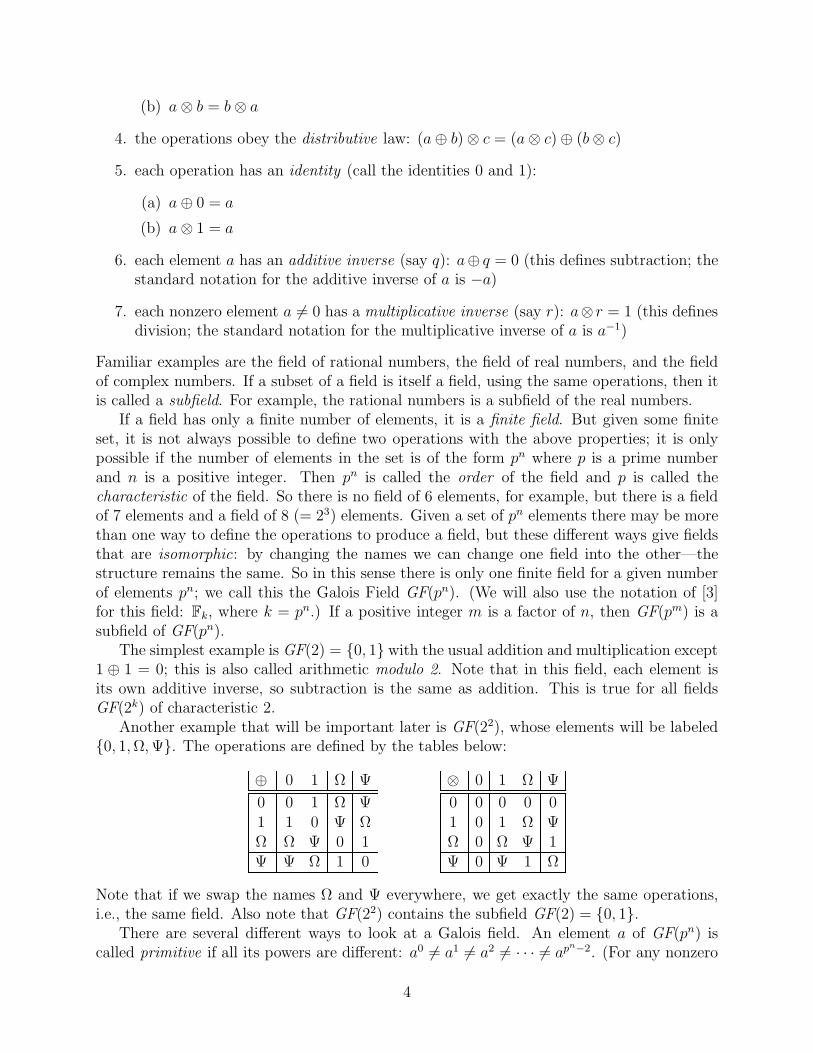
Another example that will be important later is GF(22), whose elements will be labeled0, 1, Ω, Ψ. The operations are defined by the tables below:
⊕ 0 1 Ω Ψ
0 0 1 Ω Ψ1 1 0 Ψ ΩΩ Ω Ψ 0 1Ψ Ψ Ω 1 0
⊗ 0 1 Ω Ψ
0 0 0 0 01 0 1 Ω ΨΩ 0 Ω Ψ 1Ψ 0 Ψ 1 Ω
Note that if we swap the names Ω and Ψ everywhere, we get exactly the same operations,i.e., the same field. Also note that GF(22) contains the subfield GF(2) = 0, 1.
There are several different ways to look at a Galois field. An element a of GF(pn) iscalled primitive if all its powers are different: a0 6= a1 6= a2 6= · · · 6= apn−2. (For any nonzero
4

element b then bpn−1 = 1; for any element b then bpn= b.) Hence the powers of a primitive
element give all the nonzero elements of GF(pn). Every finite field has at least one primitiveelement, so one way to look at the field is in terms of powers of that element. For example,in GF(22), Ω is a primitive element: 1 = Ω0, Ω = Ω1, Ψ = Ω2. This viewpoint makesmultiplication easy: add the exponents modulo pn − 1. But then addition is less obvious.
Another viewpoint involves polynomials, in some variable x, with coefficients in GF(p);these are called polynomials over GF(p). Each element of GF(pn) can be considered a poly-nomial over GF(p), of degree less than n. Then addition just means adding the coefficientsmodulo p. Multiplication must be done modulo some specified polynomial q(x), of degree n,with leading coefficient equal to 1; also q(x) must be irreducible, which means it is not theproduct of two polynomials of lower order.
For example, in GF(22) the only choice for q(x) is x2 + x + 1 (because the others factor:x2 = x∗x, x2+x = x∗(x+1), x2+1 = (x+1)∗(x+1); remember the coefficient arithmetic ismodulo 2). Then we could think of GF(22) as 0, 1, x, x+1 where x⊗x = (x2 modulo q) =x2 ⊕ (x2 + x + 1) = x + 1, and similarly x ⊗ (x + 1) = (x2 + x) ⊕ (x2 + x + 1) = 1 and(x + 1) ⊗ (x + 1) = (x2 + 1) ⊕ (x2 + x + 1) = x.
This polynomial viewpoint makes more sense if we think of the variable x as being a rootof the polynomial, so q(x) = 0. Then adding or subtracting multiples of q(x) is just addingzero. In the first representation of GF(22), note that Ω2 ⊕ (Ω⊕ 1) = Ψ⊕Ψ = 0, so we couldidentify x = Ω. Alternatively, we could identify x = Ψ (switching the names as before), theother root.
Another viewpoint is that the field GF(pn) is a vector space of dimension n, with vectoraddition ⊕ and multiplication by scalars in GF(p) (i.e., modulo p). (The vector viewpointis convenient for choosing a representation, but does not fully reflect the multiplicationoperation ⊗.) Then any n linearly independent elements b1, b2, . . . , bn of GF(pn) gives abasis, and we can indicate any element a by its list of coefficients with respect to this basis:if a = c1 ⊗ b1 ⊕ c2 ⊗ b2 ⊕ . . .⊕ cn ⊗ bn (with each ci ∈ GF(p)) then a is represented by the listof numbers [c1, c2, . . . , cn]. For small p this list commonly is written as digits in positionalnotation: c1c2 . . . cn.
For example, the polynomial viewpoint for GF(22), with x = Ω, corresponds to using theordered basis [Ω1, Ω0]; this is called a polynomial basis. Using this basis: 0 = 0Ω1+0Ω0 ≡ 00,1 = 0Ω1 + 1Ω0 ≡ 01, Ω = 1Ω1 + 0Ω0 ≡ 10, Ψ = 1Ω1 + 1Ω0 ≡ 11. This defines a field of 2-bitbinary numbers (where ⊕ is bitwise exclusive-or), where for example 11 ⊗ 11 = 10.
But different choices of basis are also possible. Another type of basis with convenientproperties is called a normal basis, of the form bp0
, bp1, . . . , bpn−1, where the element b of
GF(pn) must be chosen to make that set of powers linearly independent. (One nice propertyis that an isomorphism [name change] on the field has the same effect as rotating this list ofbasis elements.)
Using the ordered normal basis [Ω21, Ω20
] = [Ψ, Ω] for GF(22) gives the correspondence0 = 0Ψ + 0Ω ≡ 00, 1 = 1Ψ + 1Ω ≡ 11, Ω = 0Ψ + 1Ω ≡ 01, Ψ = 1Ψ + 0Ω ≡ 10. This givesa different 2-bit representation of GF(22); addition ⊕ is still bitwise exclusive-or, but nowfor example 11 ⊗ 11 = 11. So in one sense this is a different field, but it has exactly thesame structure as the previous version, only the names have been changed to confuse theinnocent.
The polynomial representation idea can be generalized. For any finite field F (of char-
5

acteristic p) containing a subfield S, where S is of order r = pj and F is of order rk = pjk,then the elements of F can be represented as polynomials of degree less than k, with co-efficients in S (i.e., polynomials over S). We notate this view of the field as F/S (read asF “over” S). Again, addition just means adding the coefficients in S, and multiplication isdone modulo some polynomial q(x), of degree k. The coefficients of q(x) also belong to S,with the leading coefficient equal to 1, and q(x) must be irreducible over S (no element ofS is a root). For example, the elements of GF(56) can be represented as polynomials of theform c2x
2 + c1x+ c0, with all the ci ∈ GF(52), modulo the polynomial q(x) = x3 +x2 +x+3,which is irreducible over GF(52).
Since the names of the elements of GF(pn) change with choice of representation, wemight wonder if the elements have certain properties that are independent of representation,a sort of identification. One such property is the minimal polynomial (over GF(p)) of a givenelement a. This is the irreducible polynomial of smallest degree, with coefficients in GF(p)and leading coefficient = 1, having a as a root. The degree m of the minimal polynomial isalways ≤ n, and that minimal polynomial has m distinct roots in GF(pn). Elements with thesame minimal polynomial are called conjugates; if one of them is a then the m conjugates area, ap, ap2
, . . . , apm−1. Each isomorphism of GF(pn) corresponds to replacing each element bby bpk
(for some integer k), and so in effect rotates each set of conjugates. For any primitiveelement, the minimal polynomial is called a primitive polynomial and has degree n. (Notethat a normal basis is a set of n distinct conjugates.) In GF(22) for example, the minimalpolynomial for 0 is x, that for 1 is x + 1, and the one for Ω and Ψ is x2 + x + 1 (they areconjugate primitive elements).
Again, these ideas can be extended to elements of F = GF(pn) as polynomials over anysubfield S of order r = pj, where n = jk for some k, so F is of order rk. Then each element aof F has a minimal polynomial over S, of degree m ≤ k, with m distinct roots in F , and them conjugates of a over S are a, ar, ar2
, . . . , arm−1. Also F/S is a vector space of dimensionk over S, and a normal basis is a set of k distinct conjugates.
The trace of a over S is then defined as
TrF/S(a) ≡ a + ar + ar2
+ . . . + ark−1
and the norm is defined as
NF/S(a) ≡ a · ar · ar2 · . . . · ark−1
(If the minimal polynomial of a is of degree k, then the trace is the sum of the conjugatesand the norm is the product of the conjugates.) It turns out that both the trace and thenorm are always elements of the subfield S. For example, in GF(22)/GF(2), both the traceand the norm of Ω are 1.
This brief introduction to Galois fields only covers the points relevant to the algorithmbelow. A nice, succinct introduction is given in [4]; for more depth and rigor, see [3].
3 S-box Algorithm
The S-box function of an input byte a is defined by two substeps:
6
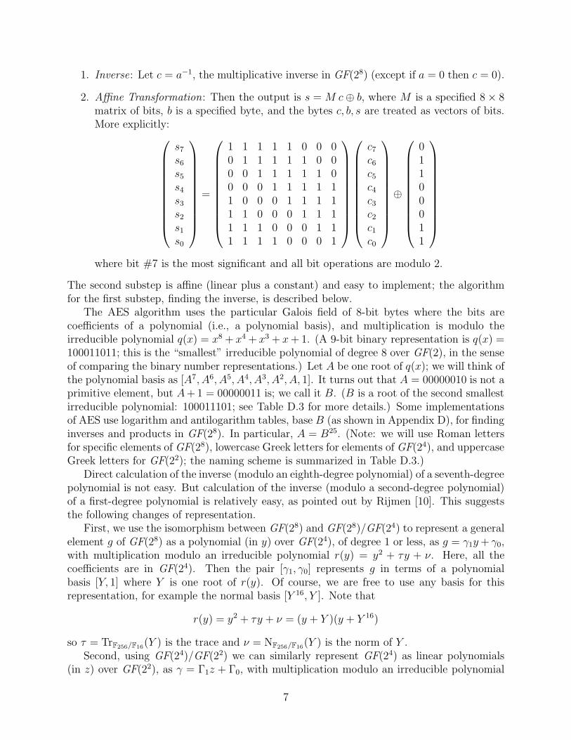
1. Inverse: Let c = a−1, the multiplicative inverse in GF(28) (except if a = 0 then c = 0).
2. Affine Transformation: Then the output is s = M c ⊕ b, where M is a specified 8 × 8matrix of bits, b is a specified byte, and the bytes c, b, s are treated as vectors of bits.More explicitly:
s7
s6
s5
s4
s3
s2
s1
s0
=
1 1 1 1 1 0 0 00 1 1 1 1 1 0 00 0 1 1 1 1 1 00 0 0 1 1 1 1 11 0 0 0 1 1 1 11 1 0 0 0 1 1 11 1 1 0 0 0 1 11 1 1 1 0 0 0 1
c7
c6
c5
c4
c3
c2
c1
c0
⊕
01100011
where bit #7 is the most significant and all bit operations are modulo 2.
The second substep is affine (linear plus a constant) and easy to implement; the algorithmfor the first substep, finding the inverse, is described below.
The AES algorithm uses the particular Galois field of 8-bit bytes where the bits arecoefficients of a polynomial (i.e., a polynomial basis), and multiplication is modulo theirreducible polynomial q(x) = x8 + x4 + x3 + x + 1. (A 9-bit binary representation is q(x) =100011011; this is the “smallest” irreducible polynomial of degree 8 over GF(2), in the senseof comparing the binary number representations.) Let A be one root of q(x); we will think ofthe polynomial basis as [A7, A6, A5, A4, A3, A2, A, 1]. It turns out that A = 00000010 is not aprimitive element, but A + 1 = 00000011 is; we call it B. (B is a root of the second smallestirreducible polynomial: 100011101; see Table D.3 for more details.) Some implementationsof AES use logarithm and antilogarithm tables, base B (as shown in Appendix D), for findinginverses and products in GF(28). In particular, A = B25. (Note: we will use Roman lettersfor specific elements of GF(28), lowercase Greek letters for elements of GF(24), and uppercaseGreek letters for GF(22); the naming scheme is summarized in Table D.3.)
Direct calculation of the inverse (modulo an eighth-degree polynomial) of a seventh-degreepolynomial is not easy. But calculation of the inverse (modulo a second-degree polynomial)of a first-degree polynomial is relatively easy, as pointed out by Rijmen [10]. This suggeststhe following changes of representation.
First, we use the isomorphism between GF(28) and GF(28)/GF(24) to represent a generalelement g of GF(28) as a polynomial (in y) over GF(24), of degree 1 or less, as g = γ1y + γ0,with multiplication modulo an irreducible polynomial r(y) = y2 + τy + ν. Here, all thecoefficients are in GF(24). Then the pair [γ1, γ0] represents g in terms of a polynomialbasis [Y, 1] where Y is one root of r(y). Of course, we are free to use any basis for thisrepresentation, for example the normal basis [Y 16, Y ]. Note that
r(y) = y2 + τy + ν = (y + Y )(y + Y 16)
so τ = TrF256/F16(Y ) is the trace and ν = NF256/F16
(Y ) is the norm of Y .Second, using GF(24)/GF(22) we can similarly represent GF(24) as linear polynomials
(in z) over GF(22), as γ = Γ1z + Γ0, with multiplication modulo an irreducible polynomial
7
s(z) = z2 + Tz + N , with all the coefficients in GF(22). Again, this uses a polynomial basis[Z, 1] for GF(24)/GF(22), where Z is one root of s(z). We could use any basis, such as thenormal basis [Z4, Z]. And for the same reasons above, T = TrF16/F4
(Z) is the trace andN = NF16/F4(Z) is the norm of Z (considering T and N as uppercase Greek for τ and ν).
Third we use GF(22)/GF(2) to represent GF(22) as linear polynomials (in w) over GF(2),as Γ = g1w + g0, with multiplication modulo t(w) = w2 + w + 1, where g1, g0 ∈ 0, 1. Thisuses a polynomial basis [W, 1], where W is either Ω or Ψ; a normal basis would be [W 2, W ].(Note that the trace and norm of Ω and Ψ are 1.)
This allows operations in GF(28) to be expressed in terms of simpler operations in GF(24),which in turn are expressed in the simple operations of GF(22). In particular, we want tofind the inverse in GF(28). Say the inverse of g = γ1y + γ0 is d = δ1y + δ0. Then (recallingsubtraction is the same as addition in GF(2n))
gd = (γ1y + γ0)(δ1y + δ0) mod (y2 + τy + ν)
= [(γ1δ1)y2 + (γ1δ0 + γ0δ1)y + (γ0δ0)] mod (y2 + τy + ν)
= [(γ1δ1)y2 + (γ1δ0 + γ0δ1)y + (γ0δ0)] + (γ1δ1)(y
2 + τy + ν)
= (γ1δ0 + γ0δ1 + γ1δ1τ)y + (γ0δ0 + γ1δ1ν)
= 1 = 0y + 1
Solving the two equations
0 = γ1δ0 + (γ0 + γ1τ)δ1
1 = γ0δ0 + (γ1ν)δ1
by
0 = γ1γ0δ0 + (γ20 + γ1γ0τ)δ1
γ1 = γ1γ0δ0 + (γ21ν)δ1
gives
γ1 = (γ21ν + γ1γ0τ + γ2
0)δ1
γ1δ0 = (γ0 + γ1τ)δ1
so that
δ1 = (γ21ν + γ1γ0τ + γ2
0)−1 γ1
δ0 = (γ21ν + γ1γ0τ + γ2
0)−1 (γ0 + γ1τ)
So finding an inverse in GF(28) involves an inverse and several multiplications in GF(24).(Addition in GF(24) as 4-bit elements, using any basis, is just bitwise exclusive-or.)
Similarly, to find the inverse in GF(24) of γ = Γ1z + Γ0 as δ = ∆1z + ∆0, then
γδ = (Γ1∆0 + Γ0∆1 + Γ1∆1T )z + (Γ0∆0 + Γ1∆1N)
8
so
∆1 = (Γ21N + Γ1Γ0T + Γ2
0)−1 Γ1
∆0 = (Γ21N + Γ1Γ0T + Γ2
0)−1 (Γ0 + Γ1T )
And to find the inverse in GF(22) of Γ = g1w + g0 as ∆ = d1w + d0, then
Γ∆ = (g1d0 + g0d1 + g1d1)w + (g0d0 + g1d1)
so
d1 = (g21 + g1g0 + g2
0)−1 g1
d0 = (g21 + g1g0 + g2
0)−1 (g0 + g1)
since both coefficients (trace and norm) in the polynomial t(w) are 1. This can be furthersimplified because for g ∈ GF(2), g2 = g−1 = g, so
d1 = (g1 + g1g0 + g0) g1
= (g1 + g1g0 + g1g0)
= g1
d0 = (g1 + g1g0 + g0) (g0 + g1)
= (g1g0 + g1 + g1g0 + g1g0 + g0 + g1g0)
= g1 + g0
Note that if the above inversion formulas are applied to a zero input then the output willalso be zero, so that special case is handled automatically.
How do these calculations change if we use normal bases at each level? In GF(28), tofind the inverse of g = γ1Y
16 +γ0Y as d = δ1Y16 + δ0Y , we use the fact that both Y and Y 16
satisfy y2 + τy + ν = 0 where τ = Y 16 + Y and ν = (Y 16)Y . Then 1 = τ−1(Y 16 + Y ), so:
gd = (γ1Y16 + γ0Y )(δ1Y
16 + δ0Y )
= (γ1δ1)(Y16)2 + (γ1δ0 + γ0δ1)(Y
16)Y + (γ0δ0)Y2
= (γ1δ1)(τY 16 + ν) + (γ1δ0 + γ0δ1)ν + (γ0δ0)(τY + ν)
= (γ1δ1τ)Y 16 + (γ0δ0τ)Y + [(γ1δ1)ν + (γ1δ0 + γ0δ1)ν + (γ0δ0)ν)]
= (γ1δ1τ)Y 16 + (γ0δ0τ)Y + [(γ1 + γ0)(δ1 + δ0)ν]τ−1(Y 16 + Y )
= [γ1δ1τ + (γ1 + γ0)(δ1 + δ0)ντ−1]Y 16 + [γ0δ0τ + (γ1 + γ0)(δ1 + δ0)ντ−1]Y
= 1 = τ−1(Y 16 + Y )
Solving the two equations
τ−1 = γ1δ1τ + (γ1 + γ0)(δ1 + δ0)ντ−1
τ−1 = γ0δ0τ + (γ1 + γ0)(δ1 + δ0)ντ−1
9
gives
0 = γ1δ1 + γ0δ0
1 = γ1δ1τ2 + (γ1δ0 + γ0δ1)ν
γ0 = γ1γ0δ1τ2 + (γ1γ0δ0 + γ2
0δ1)ν
= γ1γ0δ1τ2 + (γ2
1δ1 + γ20δ1)ν
= [γ1γ0τ2 + (γ2
1 + γ20)ν]δ1
so that
δ1 = [γ1γ0τ2 + (γ2
1 + γ20)ν]−1 γ0
δ0 = [γ1γ0τ2 + (γ2
1 + γ20)ν]−1 γ1
Again, finding an inverse in GF(28) involves an inverse and several multiplications in GF(24).Analogously, to find the inverse in GF(24) of γ = Γ1Z
4 + Γ0Z as δ = ∆1Z4 + ∆0Z, then
γδ = [Γ1∆1T + (Γ1 + Γ0)(∆1 + ∆0)NT−1]Z4 + [Γ0∆0T + (Γ1 + Γ0)(∆1 + ∆0)NT−1]Z
so
∆1 = [Γ1Γ0T2 + (Γ2
1 + Γ20)N ]−1 Γ0
∆0 = [Γ1Γ0T2 + (Γ2
1 + Γ20)N ]−1 Γ1
And to find the inverse in GF(22) of Γ = g1W2 + g0W as ∆ = d1W
2 + d0W , then
Γ∆ = [g1d1 + (g1 + g0)(d1 + d0)]W2 + [g0d0 + (g1 + g0)(d1 + d0)]W
so
d1 = [g1g0 + g1 + g0] g0
= g0
d0 = [g1g0 + g1 + g0] g1
= g1
using the same simplifications as before in GF(2).This shows how we break one problem (the 8-bit inverse in GF(28)) down into simpler
problems (4-bit operations in GF(24)), which can further be broken down to still simplerproblems (2-bit operations in GF(22) and bit operations in GF(2)).
4 Optimizations
There are several ways to reorganize the calculations above in order to reduce the totaloperation count and hence minimize the circuitry required. Additionally, there is somefreedom in the choice of the coefficients in the minimal polynomials r(y) and s(z) to giveconvenient multipliers.
10

ν⊗ γ2
γ−1
⊗
⊗
⊗ ⊕ ⊕ 4
4
γ0
γ1
δ0
δ1
Figure 1: Polynomial GF(28) inverter: (γ1y + γ0)−1 = (δ1y + δ0) Notes: the datapaths all
have the same bit width, shown at the output (4 bits here); addition is bitwise exclusive-OR;and sub-field multipliers appear below.
⊗
⊗
⊗ ⊕ ⊕
Ν⊗ Γ2
Γ−1 2
2Γ1
Γ0
∆1
∆0
Figure 2: Polynomial GF(24) inverter: (Γ1z + Γ0)−1 = (∆1z + ∆0)
The inverse formulas in GF(28)/GF(24) would simplify considerably if we could chooseτ = 0 or ν = 0, but neither choice gives an irreducible polynomial. We can find irreduciblepolynomials with τ = 1, which is also convenient. This is better than choosing ν = 1, sinceτ appears in two products in the inverse (in the polynomial basis, but even for the normalbasis τ = 1 turns out to be preferable). We can’t choose both ν = τ = 1 since then we getthe minimal polynomial of Ω and Ψ in GF(22), a subfield of GF(24). So from here on we letτ = 1 and similarly let T = 1.
4.1 Polynomial Basis Optimizations
First we consider optimizations using polynomial bases. In GF(28)/GF(24) the only op-eration required is the inverse. Satoh et al.[12] indicate the following steps in invertingg = γ1y + γ0, where we return to the ⊕,⊗ notation, and give names to intermediate results,to clarify the subfield operations needed:
φ = γ1 ⊕ γ0
θ = [(ν ⊗ γ21) ⊕ (φ ⊗ γ0)]
−1
g−1 = [θ ⊗ γ1]y + [θ ⊗ φ]
(Note: in the notation of [12], our ν becomes λ and our N becomes φ.) The operationsrequired in the subfield GF(24)/GF(22) include an inverter, multipliers, and adders (bitwiseXOR); see Figure 1.
The subfield inversions can be performed similarly, as suggested by [12]. So to invertγ = Γ1z + Γ0 in GF(24):
Φ = Γ1 ⊕ Γ0
Θ = [(N ⊗ Γ21) ⊕ (Φ ⊗ Γ0)]
−1
γ−1 = [Θ ⊗ Γ1]z + [Θ ⊗ Φ]
11

⊕ 1
1
g0
g1
d0
d1
Figure 3: Polynomial GF(22) inverter: (g1w+g0)−1 = (d1w+d0) Note: in GF(22) inverting
is the same as squaring.
⊕
⊕
⊕
⊕
Ν⊗ Γ⊗
⊗
⊗ 2
2
Γ1
Γ0
∆1
∆0
Φ1
Φ0
Figure 4: Polynomial GF(24) multiplier: (Γ1z + Γ0) ⊗ (∆1z + ∆0) = (Φ1z + Φ0)
(see Figure 2). And in GF(22) the inverse of Γ = g1w + g0 is simply:
Γ−1 = [g1]w + [g1 ⊕ g0]
(see Figure 3).The multiplier in GF(24) given by [12] finds the product γδ = (Γ1z + Γ0)(∆1z + ∆0) by
the steps
Φ = Γ0 ⊗ ∆0
γδ = [Φ ⊕ (Γ1 ⊕ Γ0) ⊗ (∆1 ⊕ ∆0)]z + [Φ ⊕ (N ⊗ Γ1 ⊗ ∆1)]
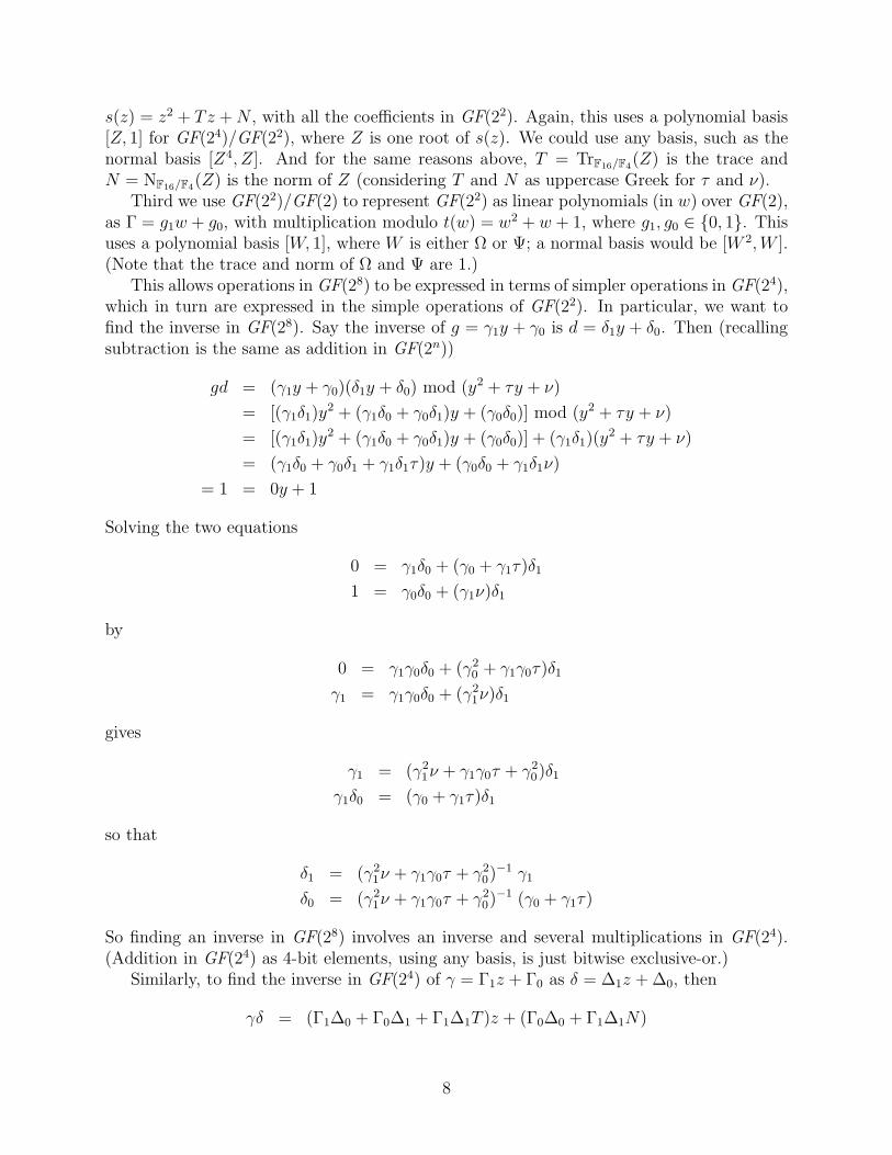
(see Figure 4.) Similarly in GF(22), the product Γ∆ = (g1w + g0)(d1w +d0) can be found by
f = g0 ⊗ d0
Γ∆ = [f ⊕ (g1 ⊕ g0) ⊗ (d1 ⊕ d0)]w + [f ⊕ (g1 ⊗ d1)]
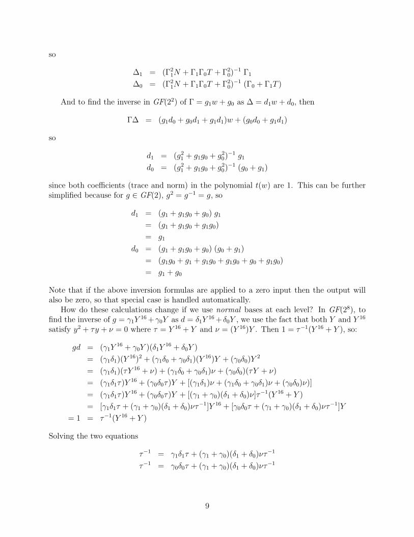
(where in GF(2), ⊗ means AND; see Figure 5).For further efficiency, multiplication by a known constant (e.g. ν above), which we will
call “scaling,” should use a specialized circuit instead of a generic multiplier, and the sameis true for squaring.
Scaling γ = Γ1z+Γ0 in GF(24) by ν = ∆1z+∆0 becomes simpler for special choices of ν,for example, if ∆0 = 0. (It is not possible to choose ∆1 = 0, because then r(y) is reducible.)Then
νγ = [∆1 ⊗ (Γ1 ⊕ Γ0)]z + [(N∆1) ⊗ Γ1]
And choosing N = ∆−11 makes scaling by ν even simpler:
νγ = [(N−1) ⊗ (Γ1 ⊕ Γ0)]z + [Γ1]
12
⊕
⊕
⊕
⊕
⊗
⊗
⊗ 1
1g0
g1
d0
d1 f0
f1
Figure 5: Polynomial GF(22) multiplier: (g1w + g0) ⊗ (d1w + d0) = (f1w + f0) Note: inGF(2), multiplication is bitwise AND.
⊕ 1
1
g0
g1
d0
d1
Figure 6: Polyno-mial GF(22) w-scaler:(w)⊗(g1w+g0) = (d1w+d0)
⊕ 1
1
g0
g1
d0
d1
Figure 7: Polyno-mial GF(22) w2-scaler:(w2)⊗(g1w+g0) = (d1w+d0)
In GF(22), since N 6= 0, 1 (so that s(z) = z2 + z + N is irreducible over GF(22)), thenboth N and N + 1 are roots of t(w) = w2 + w + 1, and N−1 = N2 = N + 1. Dependingon which root we choose for the polynomial basis [w, 1], then either N = w or N2 = w. Ineither case, since we need scalers for both N and N2, this corresponds to scalers for both wand w2, and scaling becomes
(w) ⊗ (g1w + g0) = [g1 ⊕ g0]w + [g1]
(w2) ⊗ (g1w + g0) = [g0]w + [g0 ⊕ g1]
(see Figures 6–7).Squaring γ = Γ1z ⊕ Γ0 in GF(24) corresponds to
Φ = Γ21
γ2 = [Φ]z + [Γ20 ⊕ N ⊗ Φ]
Of course, squaring Γ = g1w + g0 in the subfield GF(22) can be done similarly, using furthersimplifications in GF(2):
Γ2 = [g1]w + [g0 ⊕ g1]
Note that, in GF(22), every nonzero element Γ satisfies Γ3 = 1, so Γ−1 = Γ2, i.e., the GF(22)inverter is the same as the squarer (see Figure 3).
Another improvement comes from combining the square in GF(24) with the scaling by ν,since it is only this combination that is required in the GF(28) inverter. Then for the choice
13

1
1
g0
g1
d0
d1
Figure 8: PolynomialGF(22) square-scaler:(w)⊗(g1w+g0)
2 = (d1w+d0)Note: no gates required.
⊕ 1
1g0
g1
d0
d1
Figure 9: PolynomialGF(22) square-scaler:(w2) ⊗ (g1w + g0)
2 =(d1w + d0)
of ν above
ν ⊗ γ2 = ν ⊗ (Γ1z + Γ0)2
= ν ⊗ ([Γ21]z + [Γ2
0 ⊕ N ⊗ Γ21])
= [N2 ⊗ (Γ21 ⊕ (Γ2
0 ⊕ N ⊗ Γ21))]z + [Γ2
1]
= [(N2 + 1) ⊗ Γ21 ⊕ N2 ⊗ Γ2
0]z + [Γ21]
= [N ⊗ Γ21 ⊕ N2 ⊗ Γ2
0]z + [Γ21]
In the subfield GF(22), combining squaring with scaling by w gives
(w) ⊗ Γ2 = (w) ⊗ (g1w + g0)2
= (w) ⊗ ([g1]w + [g0 ⊕ g1])
= [g1 ⊕ (g0 ⊕ g1)]w + [g1]
= [g0]w + [g1]
(see Figure 8) so this combination is free (being just a swap of two bits)! This suggests thatif we choose w = N , then
ν ⊗ γ2 = [N ⊗ Γ21 ⊕ N ⊗ N ⊗ Γ2
0]z + [N2 ⊗ N ⊗ Γ21]
performs this combined operation with one addition and two scalings in the subfield, sincethe operations in are free. Or, if instead we choose w = N2 (see Figure 9) then
ν ⊗ γ2 = [N2 ⊗ N2 ⊗ Γ21 ⊕ N2 ⊗ Γ2
0]z + [N ⊗ N2 ⊗ Γ21]
again requiring only one addition and two scalings.Also, combining the multiplication in GF(22) with scaling by N gives a small improve-
ment; this combination appears in the GF(24) multiplier. If N = w, for example, the scaledproduct NΓ∆ = w(g1w + g0)(d1w + d0) becomes
f = (g1 ⊕ g0) ⊗ (d1 ⊕ d0)
NΓ∆ = [f ⊕ (g1 ⊗ d1)]w + [f ⊕ (g0 ⊗ d0)]
so the scaling is “free.”
14
1
1
g0
g1
d0
d1
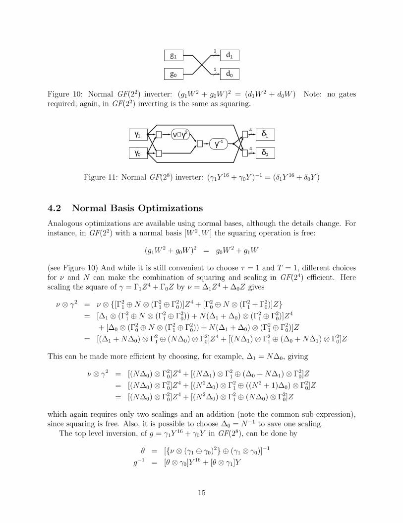
Figure 10: Normal GF(22) inverter: (g1W2 + g0W )2 = (d1W
2 + d0W ) Note: no gatesrequired; again, in GF(22) inverting is the same as squaring.
ν⊗ γ2
γ−1
⊗
⊗
⊗ ⊕
⊕ 4
4
γ0
γ1
δ0
δ1
Figure 11: Normal GF(28) inverter: (γ1Y16 + γ0Y )−1 = (δ1Y
16 + δ0Y )
4.2 Normal Basis Optimizations
Analogous optimizations are available using normal bases, although the details change. Forinstance, in GF(22) with a normal basis [W 2, W ] the squaring operation is free:
(g1W2 + g0W )2 = g0W
2 + g1W
(see Figure 10) And while it is still convenient to choose τ = 1 and T = 1, different choicesfor ν and N can make the combination of squaring and scaling in GF(24) efficient. Herescaling the square of γ = Γ1Z
4 + Γ0Z by ν = ∆1Z4 + ∆0Z gives
ν ⊗ γ2 = ν ⊗ [Γ21 ⊕ N ⊗ (Γ2
1 ⊕ Γ20)]Z
4 + [Γ20 ⊕ N ⊗ (Γ2
1 + Γ20)]Z
= [∆1 ⊗ (Γ21 ⊕ N ⊗ (Γ2
1 ⊕ Γ20)) + N(∆1 + ∆0) ⊗ (Γ2
1 ⊕ Γ20)]Z
4
+ [∆0 ⊗ (Γ20 ⊕ N ⊗ (Γ2
1 ⊕ Γ20)) + N(∆1 + ∆0) ⊗ (Γ2
1 ⊕ Γ20)]Z
= [(∆1 + N∆0) ⊗ Γ21 ⊕ (N∆0) ⊗ Γ2
0]Z4 + [(N∆1) ⊗ Γ2
1 ⊕ (∆0 + N∆1) ⊗ Γ20]Z
This can be made more efficient by choosing, for example, ∆1 = N∆0, giving
ν ⊗ γ2 = [(N∆0) ⊗ Γ20]Z
4 + [(N∆1) ⊗ Γ21 ⊕ (∆0 + N∆1) ⊗ Γ2
0]Z
= [(N∆0) ⊗ Γ20]Z
4 + [(N2∆0) ⊗ Γ21 ⊕ ((N2 + 1)∆0) ⊗ Γ2
0]Z
= [(N∆0) ⊗ Γ20]Z
4 + [(N2∆0) ⊗ Γ21 ⊕ (N∆0) ⊗ Γ2
0]Z
which again requires only two scalings and an addition (note the common sub-expression),since squaring is free. Also, it is possible to choose ∆0 = N−1 to save one scaling.
The top level inversion, of g = γ1Y16 + γ0Y in GF(28), can be done by
θ = [ν ⊗ (γ1 ⊕ γ0)2 ⊕ (γ1 ⊗ γ0)]
−1
g−1 = [θ ⊗ γ0]Y16 + [θ ⊗ γ1]Y
15
⊗
⊗
⊗ ⊕
⊕ Ν⊗ Γ2
Γ−1 2
2Γ1
Γ0
∆1
∆0
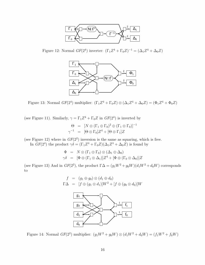
Figure 12: Normal GF(24) inverter: (Γ1Z4 + Γ0Z)−1 = (∆1Z
4 + ∆0Z)
⊕
⊕
⊕
⊕ Ν⊗ Γ
⊗
⊗
⊗ 2
2
Γ1
Γ0
∆1
∆0
Φ1
Φ0
Figure 13: Normal GF(24) multiplier: (Γ1Z4 + Γ0Z) ⊗ (∆1Z
4 + ∆0Z) = (Φ1Z4 + Φ0Z)
(see Figure 11). Similarly, γ = Γ1Z4 + Γ0Z in GF(24) is inverted by
Θ = [N ⊗ (Γ1 ⊕ Γ0)2 ⊕ (Γ1 ⊗ Γ0)]
−1
γ−1 = [Θ ⊗ Γ0]Z4 + [Θ ⊗ Γ1]Z
(see Figure 12) where in GF(22) inversion is the same as squaring, which is free.In GF(24) the product γδ = (Γ1Z
4 + Γ0Z)(∆1Z4 + ∆0Z) is found by
Φ = N ⊗ (Γ1 ⊕ Γ0) ⊗ (∆1 ⊕ ∆0)
γδ = [Φ ⊕ (Γ1 ⊗ ∆1)]Z4 + [Φ ⊕ (Γ0 ⊗ ∆0)]Z
(see Figure 13) And in GF(22), the product Γ∆ = (g1W2 + g0W )(d1W
2 + d0W ) correspondsto
f = (g1 ⊕ g0) ⊗ (d1 ⊕ d0)
Γ∆ = [f ⊕ (g1 ⊗ d1)]W2 + [f ⊕ (g0 ⊗ d0)]W
⊕
⊕
⊕
⊕
⊗
⊗
⊗ 1
1g0
g1
d0
d1 f0
f1
Figure 14: Normal GF(22) multiplier: (g1W2 + g0W ) ⊗ (d1W
2 + d0W ) = (f1W2 + f0W )
16

⊕ 1
1
g0
g1
d0
d1
Figure 15: Normal GF(22)w-scaler: (W ) ⊗ (g1W
2 +g0W ) = (d1W
2 + d0W )
⊕ 1
1
g0
g1
d0
d1
Figure 16: Normal GF(22)w2-scaler: (W 2) ⊗ (g1W
2 +g0W ) = (d1W
2 + d0W )
⊕ 1
1g0
g1
d0
d1
Figure 17: NormalGF(22) square-scaler:(W ) ⊗ (g1W
2 + g0W )2 =(d1W
2 + d0W )
⊕ 1
1
g0
g1
d0
d1
Figure 18: NormalGF(22) square-scaler:(W 2) ⊗ (g1W
2 + g0W )2 =(d1W
2 + d0W )
(see Figure 14) Scaling in GF(22) is accomplished by
(W ) ⊗ (g1W2 + g0W ) = [g1 ⊕ g0]W
2 + [g1]W
(W 2) ⊗ (g1W2 + g0W ) = [g0]W
2 + [g0 ⊕ g1]W
(see Figures 15–18)At this level of optimization, the smallest GF(28) inverter using normal bases turns out
to use exactly the same number of gates as the smallest polynomial version. However, thisdoes not account for further optimizations from common subexpressions (discussed below),nor for the change in representation (basis) required on entering and leaving the S-box.
4.3 Mixing Basis Types
There is no reason why the three bases, for GF(28), GF(24), and GF(22), should all bepolynomial bases or all be normal bases; one is free to choose either type of basis at eachlevel. (Of course, one could choose other types of basis at each level, but both polynomialand normal bases have structure that leads to efficient calculation, which is lacking in otherbases.) We have seen that the inverters in GF(28) for both types of basis require the samenumber and type of operations in GF(24), and similarly for the inverters in GF(24). Themultipliers also use the same operations for both types of bases; the same is true for thescalers in GF(22).
In GF(22), squaring is free with a normal basis, while the combination w⊗Γ2 is free witha polynomial basis. Since the GF(24) inverter needs one GF(22) inverter (same as squaring)and one combo N ⊗ Γ2, then as long as N = w this gives no preference for either type ofbasis.
The main differences then are in the combined squaring-scaling operation required bythe GF(28) inverters: ν ⊗ γ2. The details vary for the calculations this operation requires in
17

GF(22), depending on the basis types and the relations between ν, N , z, and w. The tablesbelow summarize all the different cases.
Coefficients: Polynomial GF(24) Basis XOR Gatesν = ν ⊗ (Az + B)2 = poly. GF(22) norm.
Cz + D [(CN2 + D)A2 + CB2]z + [(C + D)NA2 + DB2] w = N w = N2 GF(22)
N 0 A2 ⊕ N ⊗ B2 N2 ⊗ A2 4 5 4N2 0 N ⊗ A2 ⊕ N2 ⊗ B2 A2 4 5 4N N N2 ⊗ A2 ⊕ N ⊗ B2 N ⊗ B2 3 4 4N2 N2 A2 ⊕ N2 ⊗ B2 N2 ⊗ B2 4 4 3N 1 N ⊗ B2 (A ⊕ B)2 3 5 3N2 N N2 ⊗ B2 N ⊗ (A ⊕ B)2 3 4 4N N2 N ⊗ (A ⊕ B)2 N ⊗ (A ⊕ B)2 ⊕ B2 5 7 5N2 1 N2 ⊗ (A ⊕ B)2 N2 ⊗ (A ⊕ B)2 ⊕ N ⊗ B2 5 6 6
Coefficients: Normal GF(24) Basis XOR Gatesν = ν ⊗ (Az4 + Bz)2 = poly. GF(22) norm.
Cz4 + Dz [CA2+DN(A2+B2)]z4 + [CN(A2+B2)+DB2]z w = N w = N2 GF(22)
N 0 N ⊗ A2 N2 ⊗ (A ⊕ B)2 3 4 40 N N2 ⊗ (A ⊕ B)2 N ⊗ B2 3 4 4
N2 0 N2 ⊗ A2 (A ⊕ B)2 4 4 30 N2 (A ⊕ B)2 N2 ⊗ B2 4 4 3N 1 N ⊗ B2 N2 ⊗ A2 ⊕ N ⊗ B2 3 4 41 N N ⊗ A2 ⊕ N2 ⊗ B2 N ⊗ A2 3 4 4
N2 1 A2 ⊕ N ⊗ B2 A2 3 5 31 N2 B2 N ⊗ A2 ⊕ B2 3 5 3
The first table is for a polynomial basis in GF(24); the second is for a normal basis. Thefirst two columns show the coefficients of ν in terms of N , which depends on the bases forGF(24) and GF(22). (All eight possibilities are shown for both tables, although, due to thesymmetry of normal bases, the second table essentially has only four cases, each shown twoways.) The next two columns show the coefficients of ν⊗γ2 that need to be calculated; each isexpressed in a form to suggest a compact calculation. The last three columns show the totalnumber of XOR gates required for: a polynomial basis for GF(22) with w = N ; a polynomialbasis for GF(22) with w = N2; or a normal basis for GF(22). Note that addition in GF(22)uses two XOR’s while scaling uses one. These numbers incorporate taking advantage ofwhichever calculation is free in the particular GF(22) basis, and include this adjustment: fora polynomial basis in GF(22) with w = N2, add one since the N ⊗Γ2 in the inverter requiresa scaling.
Altogether, 85 XOR’s and 36 AND’s are needed for the rest of the calculation, so theinverter could include from 88 to 92 XOR’s (excluding common subexpression optimizationsbelow), depending on basis choice. This does not account for the gates needed to change
18
between representations (bases) on entering and exiting the S-box. Since there is only adifference of 4 XOR’s between the smallest and largest inverter that incorporate the aboveoptimizations, the change of basis can play an important role.
4.4 Common Subexpressions
A further level of optimization comes from finding subexpressions that appear more thanonce in the above hierarchical view of the inverter. Each of these common subexpressionsneed only be computed once, thus reducing the size of the inverter.
As [12] mentions, one place this occurs is when the same factor is input to two differentmultipliers. Each multiplier needs the sum of the high and low halves of each factor, soa shared factor saves one addition in the subfield. For example, a 2-bit factor shared bytwo GF(22) multipliers saves one XOR. Moreover, since each GF(24) multiplier includesthree GF(22) multipliers, then a shared 4-bit factor implies three corresponding shared 2-bitfactors. So each shared 4-bit factor saves five XOR’s (one 2-bit addition and three 1-bitadditions).
The polynomial-basis inverters for GF(28) and GF(24) each have two different factorsthat are each shared between two multipliers (which appeared as φ and θ in GF(24), Φ andΘ in GF(22)). However, each of the corresponding normal-basis inverters share all threefactors among the three multipliers (called θ, γ1 and γ0 in GF(24), and Θ, Γ1 and Γ0 inGF(22)). This gives a significant advantage to using a normal basis in GF(28), since theadditional shared factor in the GF(28) inverter saves five more XOR’s.
Another place to look is in the GF(24) square-scale combination. It turns out that, ofthe 36 variations in the tables (page 18), a repeated sum of two bits can be found in 10 cases(all with polynomial GF(24) bases), saving one XOR.
A more subtle saving occurs in the GF(24) inverter. There are essentially 6 versions,depending on the types of basis for GF(24) and GF(22), and for a polynomial GF(22) basiswhether N = w or N = w2. Each case can be improved by at least one XOR, and intwo cases, by two XOR’s. These improvements all involve bit sums computed for commonfactors being combined with some other operations, but the details vary from case to case.For example, with both bases polynomial, combining the GF(22) inverter with finding thesum of its output bits (it’s a shared factor) saves one XOR. Or for both normal bases,combining the sum of the high and low inputs and the following square-scale operation withthe bit sums of the high and low inputs (shared factors) again saves one XOR.
The last optimization occurs in the GF(28) inverter, combining the bit sums for sharedinput factors with parts of the square-scale operation. Again the details vary with thespecifics of the basis choices. All 36 versions with a normal GF(28) basis were examined (theothers have a 5 XOR handicap), and also the all-polynomial version corresponding to thebases in [12], for comparison. The resulting improvement ranges from three to five XOR’s:for most cases (23) it was three, for a dozen cases it was four, and it was five in only twocases.
While all these additional optimizations apply differently to the various basis choices,they tend to make the various versions more similar in size, with one exception: the extrashared factor in the normal GF(28) inverter gives an advantage of five XOR’s. Hence thosecases using a polynomial basis for GF(28) are effectively uncompetitive. The smallest (prior
19

to these optimizations) inverter saves 15 + 3 XOR’s in shared factors, 1 more in the GF(24)inverter, and 3 more in the GF(28) inverter, giving a total size of 66 XOR’s and 36 AND’s.(The bases of [12] give an inverter with 73 XOR’s.)
The following tables show the size of the inverter when all of these optimizations havebeen applied; in addition to the number of XOR’s shown, each inverter includes 36 AND’s.
Poly. XOR Gatesν = poly. GF(22) norm.
Cz + D w = N w = N2 GF(22)
N 0 67 67 67N2 0 67 67 67N N 67 67 67N2 N2 67 67 67N 1 67 67 67N2 N 67 67 67N N2 68 68 67N2 1 67 68 67
Norm. XOR Gatesν = poly. GF(22) norm.
Cz4 + Dz w = N w = N2 GF(22)
N 0 66 66 660 N 66 66 66
N2 0 66 66 660 N2 66 66 66N 1 66 66 661 N 66 66 66
N2 1 66 66 661 N2 66 66 66
The first table is for a polynomial GF(24) basis, the second for a normal GF(24) basis; bothtables assume a normal basis for GF(28), for the extra shared 4-bit factor. It is apparent thatthese low-level optimizations tend to even out the differences expected from the square-scaleoperation (compare with the tables on page 18). Using a polynomial GF(24) basis costsat least one XOR (one less shared 2-bit factor), and a few cases cost one more. Becausethe variation in the inverter size is so small, the cost of changing between the standardrepresentation and the S-box basis will be decisive.
4.5 Logic Gate Optimizations
Mathematically, computing the Galois inverse in GF(28) breaks down into operations inGF(2), i.e., the bitwise operations XOR and AND. However, it can be advantageous toconsider other logical operations that give equivalent results.
For example, for the 0.13-µ CMOS standard cell library considered[13], a NAND gate issmaller than an AND gate. Since the AND output bits in the GF(22) multiplier are alwayscombined by pairs in a following XOR, then the AND gates can be replaced by NAND gates.That is, [ (a ⊗ b) ⊕ (c ⊗ d) ] is equivalent to [ (a NAND b) XOR (c NAND d) ]. This gives aslight size saving.
Also, in this library an XNOR (not-exclusive-or, which really should be called NXOR)gate is the same size as an XOR gate. This is useful in the affine transformation of the S-box,where the addition of the constant b = 0x63 requires applying a NOT to some of the outputbits. In most cases, this can be done by replacing an XOR by an XNOR in the bit-matrixmultiply, so is “free.” But in some cases, such as when an output bit is given by a singleinput bit, the negation must be done explicitly with a NOT gate.
Note that the combination [ a⊕ b ⊕ (a ⊗ b) ] is equivalent to [ a OR b ]. In the few placesin the inverter where this combination occurs, we can replace 2 XOR’s and an AND by asingle OR, a worthwhile substitution. But since we use NAND’s, as mentioned above, then
20

the replacement would be a NOR, which is smaller than an OR. In fact, the NOR gate issmaller than an XOR gate, which means that even when a little rearrangement is requiredto get that combination, it is worthwhile even if the NOR ends up replacing only a singleXOR.
These gate-level optimizations apply more or less equally to the different bases considered,so play only a minor role in the selection of a particular basis.
5 Choices of Representation
This algorithm involves several related representations, or isomorphisms, of Galois Fields.First, GF(28) is considered as the set of bytes with the polynomial basis implied by theirreducible polynomial q(x) = x8 +x4 +x3 +x+1. Then GF(28)/GF(24) is also considered aspolynomials with coefficients in GF(24), based on the irreducible polynomial r(y) = y2+y+ν.Similarly, GF(24)/GF(22) uses a basis implied by the irreducible polynomial s(z) = z2+z+N ,and GF(22)/GF(2) uses a root of t(w) = w2 + w + 1. So each byte of information has twoforms: the standard AES form (polynomial basis in 8 powers of A), and the subfield formin GF(28)/GF(24) as a pair of 4-bit coefficients, each being (in GF(24)/GF(22)) a pair oftwo-bit coefficients, which in turn are coefficients in the basis for GF(22).
One approach to using these two forms, as suggested by [11], is to convert each byte of theinput block once, and do all of the AES algorithm in the new form, only converting back atthe end of all the rounds. Since all the arithmetic in the AES algorithm is Galois arithmetic,this would work fine, provided the key was appropriately converted as well. However, theMixColumns step involves multiplying by constants that are simple in the standard basis (2and 3, or A and A + 1), but this simplicity is lost in the subfield basis. For example, scalingby 2 in the standard basis takes only 3 XOR’s; the most efficient normal-basis version ofthis scaling requires 18 XOR’s. Similar concerns arise in the inverse of MixColumns, used indecryption. This extra complication more than offsets the savings from delaying the basischange back to standard. Then, as in [12], the affine transformation can be combined withthe basis change (see below). For these reasons, it is most efficient to change into the subfieldbasis on entering the S-box and to change back again on leaving it.
Each change of basis is in effect multiplication by an 8 × 8 bit matrix. Letting X referto the matrix that converts from the subfield basis to the standard basis, then to computethe S-box function of a given byte, first we do a bit-matrix multiply by X−1 to change intothe subfield basis, then calculate the Galois inverse by subfield arithmetic, then change basisback again by another bit-matrix multiply, by X. But this is followed directly by the affinetransformation (substep 2), which includes another bit-matrix multiply, by the constantmatrix M . (This can be regarded another change of basis, since M is invertible.) So we cancombine the matrices into the product MX to save one bit-matrix multiply, as pointed outby [12]. Then adding the constant b completes the S-box function.
The inverse S-box function is similar, except the XOR with constant b comes first, followedby multiplication by the bit matrix (MX)−1. Then after finding the inverse, we convert backto the standard basis through multiplication by the matrix X.
For each such constant-matrix multiply, the gate count can be reduced by “factoring out”combinations of input bits that are shared between different output bits (rows). One way to
21
do this is known as the “greedy algorithm,” where at each stage one picks the combination oftwo input bits that is shared by the most output bits; that combination is then pre-computedin a single (XOR) gate, which output effectively becomes a new input to the remaining matrixmultiply. The greedy algorithm is straightforward to implement, and generally gives goodresults.
But the greedy algorithm may not find the best result. We used a brute-force “treesearch” approach to finding the optimal factoring. At each stage, each possible choice forfactoring out a bit combination was tried, and the next stage examined recursively. Actually,some “pruning” of the tree is possible, when the bit-pair choice in the current stage isindependent of that in the calling stage and had been checked previously. Appendix C givesthe C program.
This method is guaranteed to find the minimal number of gates; the drawback is thatone cannot tell how long it will take, due to the combinatorial complexity of the algorithm.For example, running on an Intel Xeon processor under Linux (without “pruning”), oneparticular 8×8 matrix took over 2 weeks, while many others took a fraction of a microsecond.(However, many of the matrices that took very long times had already been ruled poorcandidates by the greedy algorithm, and could have been skipped.)
Using the “merged” S-box and inverse S-box of [12] complicates this picture, but reducesthe hardware required overall when both encryption and decryption are needed. There, ablock containing a single GF(28) inverter can be used to compute either the S-box functionor its inverse, depending on a selector signal. Given an input byte a, both X−1 a and(MX)−1 (a+b) are computed, with the first selected for encryption, the second for decryption.That selection is input into the inverter, and from the output byte c, both (MX) c + b andX c are computed; again the first is selected for encryption, the second for decryption.
With this merged approach, these basis-change matrix pairs can be optimized together,considering X−1 and (MX)−1 together as a 16× 8 matrix, and similarly (MX) and X, eachpair taking one byte as input and giving two bytes as output. (Then (MX)−1 (a + b) mustbe computed as (MX)−1 a + [(MX)−1 b].) Combining in this way allows more commonalityamong rows (16 instead of 8) and so yields a more compact “factored” form. Of course, thisalso means the “tree search” optimizer has a much bigger task and longer run time. (Note:this is what actually induced our development of the “pruning” strategy, which typicallygives a speedup factor of 10 to 20 times faster, enough to make full optimization feasible.)
The additive constant b of the affine transformation (or (MX)−1 b for decryption), beingan exclusive-OR with a known constant, just requires negating specific bits of the output ofthe basis change. (Actually, for the merged S-box, the multiplexors we use are themselvesnegating, so it is the bits other than those in b that need negating first.) As mentioned inSection 4.5, this usually involves replacing an XOR by an XNOR in the basis change (whichis “free” since both XOR and XNOR are the same size in the CMOS library we consider),but sometimes this is not possible and a NOT gate is required.
At this time, not all of the matrices for all of the cases considered below have been fullyoptimized, but the data so far indicate how full optimization can improve on the greedyalgorithm. For the architecture with separate encryptor and decryptor, all cases have beenfully optimized: of 1728 matrices (8 × 8) optimized, 762 (44%) were improved by at leastone XOR, and of those, 138 (18% of improved ones) were improved by two XOR’s, and 11(1.4% of improved ones) were improved by three XOR’s. For the merged architecture, the
22
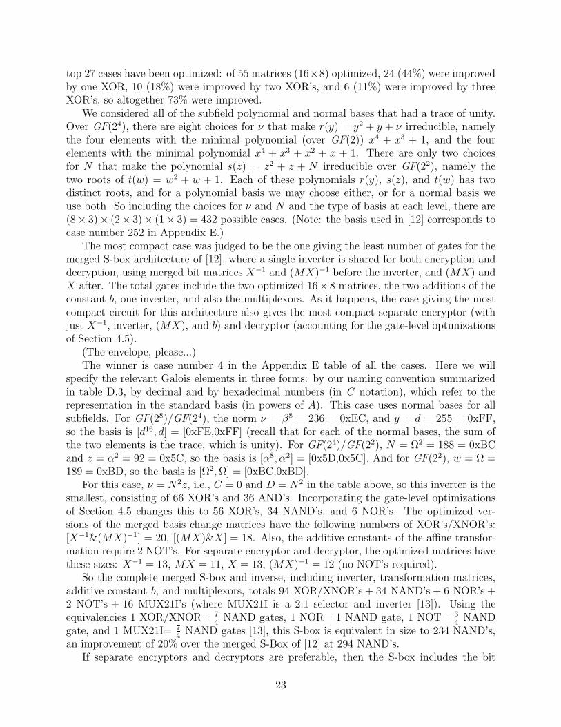
top 27 cases have been optimized: of 55 matrices (16×8) optimized, 24 (44%) were improvedby one XOR, 10 (18%) were improved by two XOR’s, and 6 (11%) were improved by threeXOR’s, so altogether 73% were improved.
We considered all of the subfield polynomial and normal bases that had a trace of unity.Over GF(24), there are eight choices for ν that make r(y) = y2 + y + ν irreducible, namelythe four elements with the minimal polynomial (over GF(2)) x4 + x3 + 1, and the fourelements with the minimal polynomial x4 + x3 + x2 + x + 1. There are only two choicesfor N that make the polynomial s(z) = z2 + z + N irreducible over GF(22), namely thetwo roots of t(w) = w2 + w + 1. Each of these polynomials r(y), s(z), and t(w) has twodistinct roots, and for a polynomial basis we may choose either, or for a normal basis weuse both. So including the choices for ν and N and the type of basis at each level, there are(8× 3)× (2× 3)× (1× 3) = 432 possible cases. (Note: the basis used in [12] corresponds tocase number 252 in Appendix E.)
The most compact case was judged to be the one giving the least number of gates for themerged S-box architecture of [12], where a single inverter is shared for both encryption anddecryption, using merged bit matrices X−1 and (MX)−1 before the inverter, and (MX) andX after. The total gates include the two optimized 16× 8 matrices, the two additions of theconstant b, one inverter, and also the multiplexors. As it happens, the case giving the mostcompact circuit for this architecture also gives the most compact separate encryptor (withjust X−1, inverter, (MX), and b) and decryptor (accounting for the gate-level optimizationsof Section 4.5).
(The envelope, please...)The winner is case number 4 in the Appendix E table of all the cases. Here we will
specify the relevant Galois elements in three forms: by our naming convention summarizedin table D.3, by decimal and by hexadecimal numbers (in C notation), which refer to therepresentation in the standard basis (in powers of A). This case uses normal bases for allsubfields. For GF(28)/GF(24), the norm ν = β8 = 236 = 0xEC, and y = d = 255 = 0xFF,so the basis is [d16, d] = [0xFE,0xFF] (recall that for each of the normal bases, the sum ofthe two elements is the trace, which is unity). For GF(24)/GF(22), N = Ω2 = 188 = 0xBCand z = α2 = 92 = 0x5C, so the basis is [α8, α2] = [0x5D,0x5C]. And for GF(22), w = Ω =189 = 0xBD, so the basis is [Ω2, Ω] = [0xBC,0xBD].
For this case, ν = N2z, i.e., C = 0 and D = N2 in the table above, so this inverter is thesmallest, consisting of 66 XOR’s and 36 AND’s. Incorporating the gate-level optimizationsof Section 4.5 changes this to 56 XOR’s, 34 NAND’s, and 6 NOR’s. The optimized ver-sions of the merged basis change matrices have the following numbers of XOR’s/XNOR’s:[X−1&(MX)−1] = 20, [(MX)&X] = 18. Also, the additive constants of the affine transfor-mation require 2 NOT’s. For separate encryptor and decryptor, the optimized matrices havethese sizes: X−1 = 13, MX = 11, X = 13, (MX)−1 = 12 (no NOT’s required).
So the complete merged S-box and inverse, including inverter, transformation matrices,additive constant b, and multiplexors, totals 94 XOR/XNOR’s + 34 NAND’s + 6 NOR’s +2 NOT’s + 16 MUX21I’s (where MUX21I is a 2:1 selector and inverter [13]). Using theequivalencies 1 XOR/XNOR= 7
4NAND gates, 1 NOR= 1 NAND gate, 1 NOT= 3
4NAND
gate, and 1 MUX21I= 74
NAND gates [13], this S-box is equivalent in size to 234 NAND’s,an improvement of 20% over the merged S-Box of [12] at 294 NAND’s.
If separate encryptors and decryptors are preferable, then the S-box includes the bit
23
matrices X−1 and MX and inverter, totaling 80 XOR’s + 34 NAND’s + 6 NOR’s, withequivalent size 180 NAND’s; the inverse S-box uses (MX)−1 and X and inverter, giving 81XOR’s + 34 NAND’s + 6 NOR’s, of size 1813
4NAND’s.
Since we have not yet fully optimized the (16 × 8) matrices for all of the 432 possiblecases, it is conceivable that one of the other cases could turn out to be better than case4. We have optimized all cases whose estimated size, based on the greedy algorithm, waswithin 9 XOR’s of the optimized size of case 4 (except in one case, where only 1 of the 2matrices was optimized; it improved by 2 XOR’s). So far, the best improvement in a single16× 8 matrix is 3 XOR’s, and the best improvement in the pair of matrices for a single caseis 5 XOR’s. For some other case to be best, full optimization must improve a matrix pair,beyond what the greedy algorithm found, by at least 10 XOR’s. We consider this highlyunlikely, and so are confident that case 4 is indeed the best of all 432 cases.
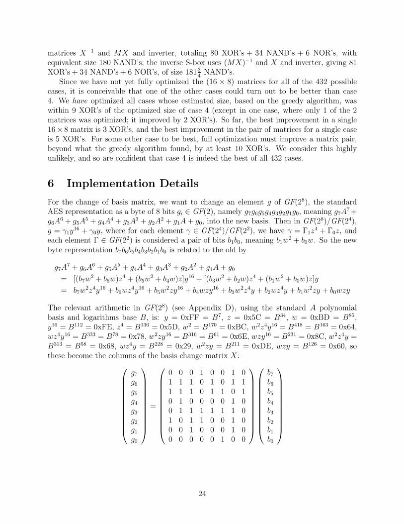
6 Implementation Details
For the change of basis matrix, we want to change an element g of GF(28), the standardAES representation as a byte of 8 bits gi ∈ GF(2), namely g7g6g5g4g3g2g1g0, meaning g7A
7 +g6A
6 + g5A5 + g4A
4 + g3A3 + g2A
2 + g1A + g0, into the new basis. Then in GF(28)/GF(24),g = γ1y
16 + γ0y, where for each element γ ∈ GF(24)/GF(22), we have γ = Γ1z4 + Γ0z, and
each element Γ ∈ GF(22) is considered a pair of bits b1b0, meaning b1w2 + b0w. So the new
byte representation b7b6b5b4b3b2b1b0 is related to the old by
g7A7 + g6A
6 + g5A5 + g4A
4 + g3A3 + g2A
2 + g1A + g0
= [(b7w2 + b6w)z4 + (b5w
2 + b4w)z]y16 + [(b3w2 + b2w)z4 + (b1w
2 + b0w)z]y
= b7w2z4y16 + b6wz4y16 + b5w
2zy16 + b4wzy16 + b3w2z4y + b2wz4y + b1w
2zy + b0wzy
The relevant arithmetic in GF(28) (see Appendix D), using the standard A polynomialbasis and logarithms base B, is: y = 0xFF = B7, z = 0x5C = B34, w = 0xBD = B85,y16 = B112 = 0xFE, z4 = B136 = 0x5D, w2 = B170 = 0xBC, w2z4y16 = B418 = B163 = 0x64,wz4y16 = B333 = B78 = 0x78, w2zy16 = B316 = B61 = 0x6E, wzy16 = B231 = 0x8C, w2z4y =B313 = B58 = 0x68, wz4y = B228 = 0x29, w2zy = B211 = 0xDE, wzy = B126 = 0x60, sothese become the columns of the basis change matrix X:
g7
g6
g5
g4
g3
g2
g1
g0
=
0 0 0 1 0 0 1 01 1 1 0 1 0 1 11 1 1 0 1 1 0 10 1 0 0 0 0 1 00 1 1 1 1 1 1 01 0 1 1 0 0 1 00 0 1 0 0 0 1 00 0 0 0 0 1 0 0
b7
b6
b5
b4
b3
b2
b1
b0
24
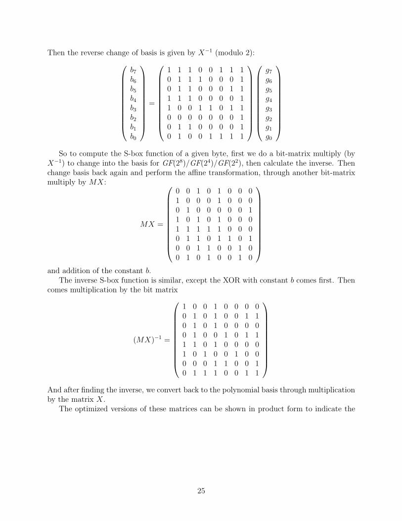
Then the reverse change of basis is given by X−1 (modulo 2):
b7
b6
b5
b4
b3
b2
b1
b0
=
1 1 1 0 0 1 1 10 1 1 1 0 0 0 10 1 1 0 0 0 1 11 1 1 0 0 0 0 11 0 0 1 1 0 1 10 0 0 0 0 0 0 10 1 1 0 0 0 0 10 1 0 0 1 1 1 1
g7
g6
g5
g4
g3
g2
g1
g0
So to compute the S-box function of a given byte, first we do a bit-matrix multiply (byX−1) to change into the basis for GF(28)/GF(24)/GF(22), then calculate the inverse. Thenchange basis back again and perform the affine transformation, through another bit-matrixmultiply by MX:
MX =
0 0 1 0 1 0 0 01 0 0 0 1 0 0 00 1 0 0 0 0 0 11 0 1 0 1 0 0 01 1 1 1 1 0 0 00 1 1 0 1 1 0 10 0 1 1 0 0 1 00 1 0 1 0 0 1 0
and addition of the constant b.The inverse S-box function is similar, except the XOR with constant b comes first. Then
comes multiplication by the bit matrix
(MX)−1 =
1 0 0 1 0 0 0 00 1 0 1 0 0 1 10 1 0 1 0 0 0 00 1 0 0 1 0 1 11 1 0 1 0 0 0 01 0 1 0 0 1 0 00 0 0 1 1 0 0 10 1 1 1 0 0 1 1
And after finding the inverse, we convert back to the polynomial basis through multiplicationby the matrix X.
The optimized versions of these matrices can be shown in product form to indicate the
25
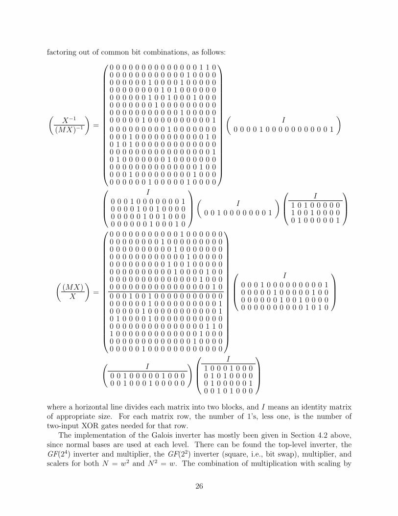
factoring out of common bit combinations, as follows:
(X−1
(MX)−1
)=
0 0 0 0 0 0 0 0 0 0 0 0 0 0 1 1 00 0 0 0 0 0 0 0 0 0 0 0 1 0 0 0 00 0 0 0 0 0 1 0 0 0 0 1 0 0 0 0 00 0 0 0 0 0 0 0 1 0 1 0 0 0 0 0 00 0 0 0 0 0 1 0 0 1 0 0 0 1 0 0 00 0 0 0 0 0 0 1 0 0 0 0 0 0 0 0 00 0 0 0 0 0 0 0 0 0 0 1 0 0 0 0 00 0 0 0 0 1 0 0 0 0 0 0 0 0 0 0 10 0 0 0 0 0 0 0 0 1 0 0 0 0 0 0 00 0 0 1 0 0 0 0 0 0 0 0 0 0 0 1 00 1 0 1 0 0 0 0 0 0 0 0 0 0 0 0 00 0 0 0 0 0 0 0 0 0 0 0 0 0 0 0 10 1 0 0 0 0 0 0 0 1 0 0 0 0 0 0 00 0 0 0 0 0 0 0 0 0 0 0 0 0 1 0 00 0 0 1 0 0 0 0 0 0 0 0 0 1 0 0 00 0 0 0 0 0 1 0 0 0 0 0 1 0 0 0 0
(I
0 0 0 0 1 0 0 0 0 0 0 0 0 0 0 1
)
I0 0 0 1 0 0 0 0 0 0 0 10 0 0 0 1 0 0 1 0 0 0 00 0 0 0 0 1 0 0 1 0 0 00 0 0 0 0 0 1 0 0 0 1 0
(
I0 0 1 0 0 0 0 0 0 0 1
)
I1 0 1 0 0 0 0 01 0 0 1 0 0 0 00 1 0 0 0 0 0 1
((MX)
X
)=
0 0 0 0 0 0 0 0 0 0 0 1 0 0 0 0 0 00 0 0 0 0 0 0 0 1 0 0 0 0 0 0 0 0 00 0 0 0 0 0 0 0 0 0 1 0 0 0 0 0 0 00 0 0 0 0 0 0 0 0 0 0 0 1 0 0 0 0 00 0 0 0 0 0 0 0 0 1 0 0 1 0 0 0 0 00 0 0 0 0 0 0 0 0 0 1 0 0 0 0 1 0 00 0 0 0 0 0 0 0 0 0 0 0 0 0 1 0 0 00 0 0 0 0 0 0 0 0 0 0 0 0 0 0 0 1 00 0 0 1 0 0 1 0 0 0 0 0 0 0 0 0 0 00 0 0 0 0 0 1 0 0 0 0 0 0 0 0 0 0 10 0 0 0 0 1 0 0 0 0 0 0 0 0 0 0 0 10 1 0 0 0 0 1 0 0 0 0 0 0 0 0 0 0 00 0 0 0 0 0 0 0 0 0 0 0 0 0 0 1 1 01 0 0 0 0 0 0 0 0 0 0 0 0 0 1 0 0 00 0 0 0 0 0 0 0 0 0 0 0 0 1 0 0 0 00 0 0 0 0 1 0 0 0 0 0 0 0 0 0 0 0 0
I0 0 0 1 0 0 0 0 0 0 0 0 0 10 0 0 0 0 1 0 0 0 0 0 1 0 00 0 0 0 0 0 1 0 0 1 0 0 0 00 0 0 0 0 0 0 0 0 0 1 0 1 0
(I
0 0 1 0 0 0 0 0 1 0 0 00 0 1 0 0 0 1 0 0 0 0 0
)
I1 0 0 0 1 0 0 00 1 0 1 0 0 0 00 1 0 0 0 0 0 10 0 1 0 1 0 0 0
where a horizontal line divides each matrix into two blocks, and I means an identity matrixof appropriate size. For each matrix row, the number of 1’s, less one, is the number oftwo-input XOR gates needed for that row.
The implementation of the Galois inverter has mostly been given in Section 4.2 above,since normal bases are used at each level. There can be found the top-level inverter, theGF(24) inverter and multiplier, the GF(22) inverter (square, i.e., bit swap), multiplier, andscalers for both N = w2 and N2 = w. The combination of multiplication with scaling by
26

⊕
Γ2 2
2Γ1
Γ0
∆1
∆0Ν⊗ Γ
Γ2
Figure 19: Normal GF(24) square-scale: ν ⊗ (Γ1Z4 + Γ0Z)2 = ∆1Z
4 + ∆0Z
N = w2 in GF(22) is given by
f = g0 ⊗ d0
NΓ∆ = [f ⊕ ((g1 ⊕ g0) ⊗ (d1 ⊕ d0))]w2 + [f ⊕ (g1 ⊗ d1)]w
The only other operation required is the square-scale operator in the normal basis GF(24),as shown on page 18 for C = 0 and D = N2, which is
ν(Az4 + Bz)2 = [(A ⊕ B)2]z4 + [N2 ⊗ B2]z
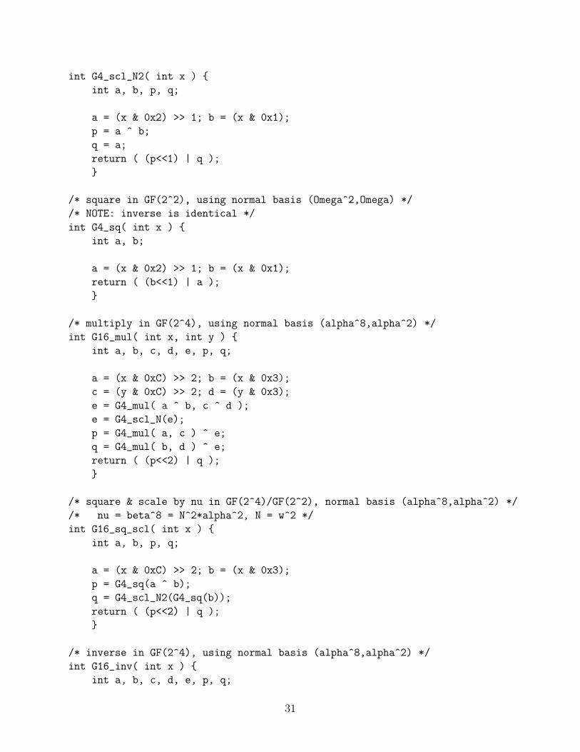
where the squaring is free (see Figure 19).Appendix A gives a C program that implements the S-box function (and its inverse) to
illustrate the algorithm. This shows the hierarchical structure of the subfield approach, butdoes not include the low-level optimizations of Section 4.4. The output is a table that can becompared with the reference version in the file boxes-ref.dat, included in the “Referencecode in ANSI C v2.2.” link from The Rijndael Page:http://www.esat.kuleuven.ac.be/~rijmen/rijndael/
Appendix B gives our compact implementation of the merged S-box and inverse as aVerilog module. All the low-level optimizations of Sections 4.4 and 4.5 are shown. Theseinclude: pre-computing sums of high and low parts of common factors for multipliers; in theGF(28) inverter, using the bit sums of common factors to replace some terms in the scaledsquare of the sum of high and low inputs; similarly in the GF(24) inverter; using NAND’sinstead of AND’s, and replacing some XOR’s and NAND’s by NOR’s.
We sucessfully tested this implementation using an FPGA (though our approach is reallymore appropriate for ASIC’s). Specifically, we used an SRC-6E Reconfigurable Computer,which includes two Intel processors and two Virtex II FPGA’s. As implemented on oneFPGA, the function evaluation takes just one tick of the 100 MHz clock, the same amountof time needed for the table look-up approach.
We also implemented a complete AES encryptor/decryptor on this same system, usingour S-box. Certain constraints (block RAM access) of this particular system prevent usingtable lookup for a fully unrolled pipelined version; 160 copies of the table (16 bytes/round×10rounds) would not fit. So for this system, our compact S-box allowed us to implement afully pipelined encryptor/decryptor, where in the FPGA, effectively one block is processedfor each clock tick.
7 Conclusion
The goal of this work is an algorithm to compute the S-box function of AES, that can beimplemented in hardware with a minimal amount of circuitry. This should save a significant
27
amount of chip area in ASIC hardware versions of AES. Moreover, this area savings couldallow many copies of the S-box circuit to fit on a chip, enough to “unroll” the loop of 10rounds. This in turn would allow the AES process to be fully pipelined, increasing the rateof throughput significantly (for non-feedback modes of encryption), on smaller chips.
This algorithm employs the multi-level representation of arithmetic in GF(28), similar tothe previous compact implementation of Satoh et al[12]. Our work shows how this approachleads to a whole family of 432 implementations, depending on the particular isomorphism(basis) chosen, from which we found the best one. And in factoring the transformation (basischange) matrices for compactness, rather than rely on the greedy algorithm as in prior work,we fully optimized the matrices, using our tree search algorithm with pruning of redundantcases. This gave an improvement over the greedy algorithm in 73% of the (16× 8) matricesthat we optimized. Also new is the detailed description of this nested-subfield algorithm,including specification of all constants for each choice of representation.
Our best compact implementation gives an S-box that is 20% smaller than the previouslymost compact version of [12]. We have shown that none of the other 431 versions possiblewith this subfield approach is as small. This compact S-box could be useful for many futurehardware implementations of AES, for a variety of security applications.
Acknowledgements
This work was supported by the National Security Agency.Many thanks to Akashi Satoh for his patient and very helpful discussions.
References
[1] Pawel Chodowiec and Kris Gaj. Very compact FPGA implementation of the AESalgorithm. In C.D. Walter et al., editor, CHES 2003, LNCS 2779, pages 319–333, 2003.
[2] Kimmo U. Jarvinen, Matti T. Tommiska, and Jorma O. Skytta. A fully pipelinedmemoryless 17.8 gbps AES128 encryptor. In FPGA 03. ACM, 2003.
[3] Rudolf Lidl and Harald Niederreiter. Introduction to finite fields and their applications.Cambridge, New York, 1986.
[4] F. J. MacWilliams and N. J. A. Sloane. The Theory of Error-Correcting Codes. North-Holland, New York, 1977.
[5] Sumio Morioka and Akashi Satoh. A 10 Gbps full-AES crypto design with a twisted-BDD S-box architecture. In IEEE International Conference on Computer Design. IEEE,2002.
[6] Sumio Morioka and Akashi Satoh. An optimized S-box circuit arthitecture for low powerAES design. In CHES2002, LNCS 2523, pages 172–186, 2003.
[7] NIST. Commerce department announces winner ofglobal information security competition. press release athttp://www.nist.gov/public_affairs/releases/g00-176.htm, October 2000.
28

[8] NIST. Recommendation for block cipher modes of operation. Technical Report SP800-38A, National Institute of Standards and Technology (NIST), December 2001.
[9] NIST. Specification for the ADVANCED ENCRYPTION STANDARD (AES). Tech-nical Report FIPS PUB 197, National Institute of Standards and Technology (NIST),November 2001.
[10] Vincent Rijmen. Efficient implementation of the Rijndael S-box. available athttp://www.esat.kuleuven.ac.be/~rijmen/rijndael/sbox.pdf.
[11] Atri Rudra, Pradeep K. Dubey, Charanjit S. Jutla, Vijay Kumar, Josyula R. Rao,and Pankaj Rohatgi. Efficient Rijndael encryption implementation with composite fieldarithmetic. In CHES2001, LNCS 2162, pages 171–184, 2001.
[12] A. Satoh, S. Morioka, K. Takano, and Seiji Munetoh. A compact Rijndael hardwarearchitecture with S-box optimization. In Advances in Cryptology - ASIACRYPT 2001,LNCS 2248, pages 239–254, 2001.
[13] Akashi Satoh. personal communication, July 2004.
[14] Nicholas Weaver and John Wawrzynek. High performance, com-pact AES implementations in Xilinx FPGAs. available athttp://www.cs.berkeley.edu/~nweaver/papers/AES_in_FPGAs.pdf, September2002.
[15] Johannes Wolkerstorfer, Elisabeth Oswald, and Mario Lamberger. An ASIC implemen-tation of the AES Sboxes. In CT-RSA 2002, LNCS 2271, pages 67–78, 2002.
29

A S-box Algorithm in C
/* sbox.c
*
* by: David Canright
*
* illustrates compact implementation of AES S-box via subfield operations
* case # 4 : [d^16, d], [alpha^8, alpha^2], [Omega^2, Omega]
* nu = beta^8 = N^2*alpha^2, N = w^2
*/
#include <stdio.h>
#include <sys/types.h>
/* to convert between polynomial (A^7...1) basis A & normal basis X */
/* or to basis S which incorporates bit matrix of Sbox */
static int
A2X[8] = 0x98, 0xF3, 0xF2, 0x48, 0x09, 0x81, 0xA9, 0xFF,
X2A[8] = 0x64, 0x78, 0x6E, 0x8C, 0x68, 0x29, 0xDE, 0x60,
X2S[8] = 0x58, 0x2D, 0x9E, 0x0B, 0xDC, 0x04, 0x03, 0x24,
S2X[8] = 0x8C, 0x79, 0x05, 0xEB, 0x12, 0x04, 0x51, 0x53;
/* multiply in GF(2^2), using normal basis (Omega^2,Omega) */
int G4_mul( int x, int y )
int a, b, c, d, e, p, q;
a = (x & 0x2) >> 1; b = (x & 0x1);
c = (y & 0x2) >> 1; d = (y & 0x1);
e = (a ^ b) & (c ^ d);
p = (a & c) ^ e;
q = (b & d) ^ e;
return ( (p<<1) | q );
/* scale by N = Omega^2 in GF(2^2), using normal basis (Omega^2,Omega) */
int G4_scl_N( int x )
int a, b, p, q;
a = (x & 0x2) >> 1; b = (x & 0x1);
p = b;
q = a ^ b;
return ( (p<<1) | q );
/* scale by N^2 = Omega in GF(2^2), using normal basis (Omega^2,Omega) */
30
int G4_scl_N2( int x )
int a, b, p, q;
a = (x & 0x2) >> 1; b = (x & 0x1);
p = a ^ b;
q = a;
return ( (p<<1) | q );
/* square in GF(2^2), using normal basis (Omega^2,Omega) */
/* NOTE: inverse is identical */
int G4_sq( int x )
int a, b;
a = (x & 0x2) >> 1; b = (x & 0x1);
return ( (b<<1) | a );
/* multiply in GF(2^4), using normal basis (alpha^8,alpha^2) */
int G16_mul( int x, int y )
int a, b, c, d, e, p, q;
a = (x & 0xC) >> 2; b = (x & 0x3);
c = (y & 0xC) >> 2; d = (y & 0x3);
e = G4_mul( a ^ b, c ^ d );
e = G4_scl_N(e);
p = G4_mul( a, c ) ^ e;
q = G4_mul( b, d ) ^ e;
return ( (p<<2) | q );
/* square & scale by nu in GF(2^4)/GF(2^2), normal basis (alpha^8,alpha^2) */
/* nu = beta^8 = N^2*alpha^2, N = w^2 */
int G16_sq_scl( int x )
int a, b, p, q;
a = (x & 0xC) >> 2; b = (x & 0x3);
p = G4_sq(a ^ b);
q = G4_scl_N2(G4_sq(b));
return ( (p<<2) | q );
/* inverse in GF(2^4), using normal basis (alpha^8,alpha^2) */
int G16_inv( int x )
int a, b, c, d, e, p, q;
31

a = (x & 0xC) >> 2; b = (x & 0x3);
c = G4_scl_N( G4_sq( a ^ b ) );
d = G4_mul( a, b );
e = G4_sq( c ^ d ); // really inverse, but same as square
p = G4_mul( e, b );
q = G4_mul( e, a );
return ( (p<<2) | q );
/* inverse in GF(2^8), using normal basis (d^16,d) */
int G256_inv( int x )
int a, b, c, d, e, p, q;
a = (x & 0xF0) >> 4; b = (x & 0x0F);
c = G16_sq_scl( a ^ b );
d = G16_mul( a, b );
e = G16_inv( c ^ d );
p = G16_mul( e, b );
q = G16_mul( e, a );
return ( (p<<4) | q );
/* convert to new basis in GF(2^8) */
/* i.e., bit matrix multiply */
int G256_newbasis( int x, int b[] )
int i, y = 0;
for ( i=7; i >= 0; i-- )
if ( x & 1 ) y ^= b[i];
x >>= 1;
return ( y );
/* find Sbox of n in GF(2^8) mod POLY */
int Sbox( int n )
int t;
t = G256_newbasis( n, A2X );
t = G256_inv( t );
t = G256_newbasis( t, X2S );
return ( t ^ 0x63 );
32

/* find inverse Sbox of n in GF(2^8) mod POLY */
int iSbox( int n )
int t;
t = G256_newbasis( n ^ 0x63, S2X );
t = G256_inv( t );
t = G256_newbasis( t, X2A );
return ( t );
/* compute tables of Sbox & its inverse; print ’em out */
int main ()
int Sbox_tbl[256], iSbox_tbl[256], i, j;
for (i = 0; i < 256; i++)
Sbox_tbl[i] = Sbox(i);
iSbox_tbl[i] = iSbox(i);
printf ("char S[256] = \n");
for (i = 0; i < 16; i++)
for (j = 0; j < 16; j++)
printf ( "%3d, ", Sbox_tbl[i*16+j]);
printf ( "\n" );
printf ( ";\n\n" );
printf ("char Si[256] = \n");
for (i = 0; i < 16; i++)
for (j = 0; j < 16; j++)
printf ( "%3d, ", iSbox_tbl[i*16+j]);
printf ( "\n" );
printf ( ";\n\n" );
return(0);
33

B S-box Algorithm in Verilog
/* S-box using all normal bases */
/* case # 4 : [d^16, d], [alpha^8, alpha^2], [Omega^2, Omega] */
/* beta^8 = N^2*alpha^2, N = w^2 */
/* optimized using OR gates and NAND gates */
/* square in GF(2^2), using normal basis [Omega^2,Omega] */
/* inverse is the same as square in GF(2^2), using any normal basis */
module GF_SQ_2 ( A, Q );
input [1:0] A;
output [1:0] Q;
assign Q = A[0], A[1] ;
endmodule
/* scale by w = Omega in GF(2^2), using normal basis [Omega^2,Omega] */
module GF_SCLW_2 ( A, Q );
input [1:0] A;
output [1:0] Q;
assign Q = (A[1] ^ A[0]), A[1] ;
endmodule
/* scale by w^2 = Omega^2 in GF(2^2), using normal basis [Omega^2,Omega] */
module GF_SCLW2_2 ( A, Q );
input [1:0] A;
output [1:0] Q;
assign Q = A[0], (A[1] ^ A[0]) ;
endmodule
/* multiply in GF(2^2), shared factors, using normal basis [Omega^2,Omega] */
module GF_MULS_2 ( A, ab, B, cd, Q );
input [1:0] A;
input ab;
input [1:0] B;
input cd;
output [1:0] Q;
wire abcd, p, q;
assign abcd = ~(ab & cd); /* note: ~& syntax for NAND won’t compile */
assign p = (~(A[1] & B[1])) ^ abcd;
assign q = (~(A[0] & B[0])) ^ abcd;
assign Q = p, q ;
34

endmodule
/* multiply & scale by N in GF(2^2), shared factors, basis [Omega^2,Omega] */
module GF_MULS_SCL_2 ( A, ab, B, cd, Q );
input [1:0] A;
input ab;
input [1:0] B;
input cd;
output [1:0] Q;
wire t, p, q;
assign t = ~(A[0] & B[0]); /* note: ~& syntax for NAND won’t compile */
assign p = (~(ab & cd)) ^ t;
assign q = (~(A[1] & B[1])) ^ t;
assign Q = p, q ;
endmodule
/* inverse in GF(2^4)/GF(2^2), using normal basis [alpha^8, alpha^2] */
module GF_INV_4 ( A, Q );
input [3:0] A;
output [3:0] Q;
wire [1:0] a, b, c, d, p, q;
wire sa, sb, sd; /* for shared factors in multipliers */
assign a = A[3:2];
assign b = A[1:0];
assign sa = a[1] ^ a[0];
assign sb = b[1] ^ b[0];
/* optimize this section as shown below
GF_MULS_2 abmul(a, sa, b, sb, ab);
GF_SQ_2 absq( (a ^ b), ab2);
GF_SCLW2_2 absclN( ab2, ab2N);
GF_SQ_2 dinv( (ab ^ ab2N), d);
*/
assign c = /* note: ~| syntax for NOR won’t compile */
~(a[1] | b[1]) ^ (~(sa & sb)) ,
~(sa | sb) ^ (~(a[0] & b[0])) ;
GF_SQ_2 dinv( c, d);
/* end of optimization */
assign sd = d[1] ^ d[0];
GF_MULS_2 pmul(d, sd, b, sb, p);
GF_MULS_2 qmul(d, sd, a, sa, q);
assign Q = p, q ;
endmodule
35
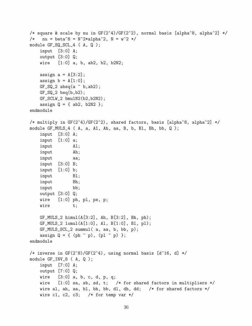
/* square & scale by nu in GF(2^4)/GF(2^2), normal basis [alpha^8, alpha^2] */
/* nu = beta^8 = N^2*alpha^2, N = w^2 */
module GF_SQ_SCL_4 ( A, Q );
input [3:0] A;
output [3:0] Q;
wire [1:0] a, b, ab2, b2, b2N2;
assign a = A[3:2];
assign b = A[1:0];
GF_SQ_2 absq(a ^ b,ab2);
GF_SQ_2 bsq(b,b2);
GF_SCLW_2 bmulN2(b2,b2N2);
assign Q = ab2, b2N2 ;
endmodule
/* multiply in GF(2^4)/GF(2^2), shared factors, basis [alpha^8, alpha^2] */
module GF_MULS_4 ( A, a, Al, Ah, aa, B, b, Bl, Bh, bb, Q );
input [3:0] A;
input [1:0] a;
input Al;
input Ah;
input aa;
input [3:0] B;
input [1:0] b;
input Bl;
input Bh;
input bb;
output [3:0] Q;
wire [1:0] ph, pl, ps, p;
wire t;
GF_MULS_2 himul(A[3:2], Ah, B[3:2], Bh, ph);
GF_MULS_2 lomul(A[1:0], Al, B[1:0], Bl, pl);
GF_MULS_SCL_2 summul( a, aa, b, bb, p);
assign Q = (ph ^ p), (pl ^ p) ;
endmodule
/* inverse in GF(2^8)/GF(2^4), using normal basis [d^16, d] */
module GF_INV_8 ( A, Q );
input [7:0] A;
output [7:0] Q;
wire [3:0] a, b, c, d, p, q;
wire [1:0] sa, sb, sd, t; /* for shared factors in multipliers */
wire al, ah, aa, bl, bh, bb, dl, dh, dd; /* for shared factors */
wire c1, c2, c3; /* for temp var */
36

assign a = A[7:4];
assign b = A[3:0];
assign sa = a[3:2] ^ a[1:0];
assign sb = b[3:2] ^ b[1:0];
assign al = a[1] ^ a[0];
assign ah = a[3] ^ a[2];
assign aa = sa[1] ^ sa[0];
assign bl = b[1] ^ b[0];
assign bh = b[3] ^ b[2];
assign bb = sb[1] ^ sb[0];
/* optimize this section as shown below
GF_MULS_4 abmul(a, sa, al, ah, aa, b, sb, bl, bh, bb, ab);
GF_SQ_SCL_4 absq( (a ^ b), ab2);
GF_INV_4 dinv( (ab ^ ab2), d);
*/
assign c1 = ~(ah & bh);
assign c2 = ~(sa[0] & sb[0]);
assign c3 = ~(aa & bb);
assign c = /* note: ~| syntax for NOR won’t compile */
(~(sa[0] | sb[0]) ^ (~(a[3] & b[3]))) ^ c1 ^ c3 ,
(~(sa[1] | sb[1]) ^ (~(a[2] & b[2]))) ^ c1 ^ c2 ,
(~(al | bl) ^ (~(a[1] & b[1]))) ^ c2 ^ c3 ,
(~(a[0] | b[0]) ^ (~(al & bl))) ^ (~(sa[1] & sb[1])) ^ c2 ;
GF_INV_4 dinv( c, d);
/* end of optimization */
assign sd = d[3:2] ^ d[1:0];
assign dl = d[1] ^ d[0];
assign dh = d[3] ^ d[2];
assign dd = sd[1] ^ sd[0];
GF_MULS_4 pmul(d, sd, dl, dh, dd, b, sb, bl, bh, bb, p);
GF_MULS_4 qmul(d, sd, dl, dh, dd, a, sa, al, ah, aa, q);
assign Q = p, q ;
endmodule
/* MUX21I is an inverting 2:1 multiplexor */
module MUX21I ( A, B, s, Q );
input A;
input B;
input s;
output Q;
assign Q = ~ ( s ? A : B ); /* mock-up for FPGA implementation */
endmodule
/* select and invert (NOT) byte, using MUX21I */
37
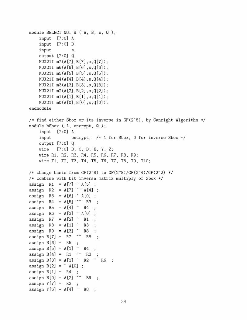
module SELECT_NOT_8 ( A, B, s, Q );
input [7:0] A;
input [7:0] B;
input s;
output [7:0] Q;
MUX21I m7(A[7],B[7],s,Q[7]);
MUX21I m6(A[6],B[6],s,Q[6]);
MUX21I m5(A[5],B[5],s,Q[5]);
MUX21I m4(A[4],B[4],s,Q[4]);
MUX21I m3(A[3],B[3],s,Q[3]);
MUX21I m2(A[2],B[2],s,Q[2]);
MUX21I m1(A[1],B[1],s,Q[1]);
MUX21I m0(A[0],B[0],s,Q[0]);
endmodule
/* find either Sbox or its inverse in GF(2^8), by Canright Algorithm */
module bSbox ( A, encrypt, Q );
input [7:0] A;
input encrypt; /* 1 for Sbox, 0 for inverse Sbox */
output [7:0] Q;
wire [7:0] B, C, D, X, Y, Z;
wire R1, R2, R3, R4, R5, R6, R7, R8, R9;
wire T1, T2, T3, T4, T5, T6, T7, T8, T9, T10;
/* change basis from GF(2^8) to GF(2^8)/GF(2^4)/GF(2^2) */
/* combine with bit inverse matrix multiply of Sbox */
assign R1 = A[7] ^ A[5] ;
assign R2 = A[7] ~^ A[4] ;
assign R3 = A[6] ^ A[0] ;
assign R4 = A[5] ~^ R3 ;
assign R5 = A[4] ^ R4 ;
assign R6 = A[3] ^ A[0] ;
assign R7 = A[2] ^ R1 ;
assign R8 = A[1] ^ R3 ;
assign R9 = A[3] ^ R8 ;
assign B[7] = R7 ~^ R8 ;
assign B[6] = R5 ;
assign B[5] = A[1] ^ R4 ;
assign B[4] = R1 ~^ R3 ;
assign B[3] = A[1] ^ R2 ^ R6 ;
assign B[2] = ~ A[0] ;
assign B[1] = R4 ;
assign B[0] = A[2] ~^ R9 ;
assign Y[7] = R2 ;
assign Y[6] = A[4] ^ R8 ;
38

assign Y[5] = A[6] ^ A[4] ;
assign Y[4] = R9 ;
assign Y[3] = A[6] ~^ R2 ;
assign Y[2] = R7 ;
assign Y[1] = A[4] ^ R6 ;
assign Y[0] = A[1] ^ R5 ;
SELECT_NOT_8 sel_in( B, Y, encrypt, Z );
GF_INV_8 inv( Z, C );
/* change basis back from GF(2^8)/GF(2^4)/GF(2^2) to GF(2^8) */
assign T1 = C[7] ^ C[3] ;
assign T2 = C[6] ^ C[4] ;
assign T3 = C[6] ^ C[0] ;
assign T4 = C[5] ~^ C[3] ;
assign T5 = C[5] ~^ T1 ;
assign T6 = C[5] ~^ C[1] ;
assign T7 = C[4] ~^ T6 ;
assign T8 = C[2] ^ T4 ;
assign T9 = C[1] ^ T2 ;
assign T10 = T3 ^ T5 ;
assign D[7] = T4 ;
assign D[6] = T1 ;
assign D[5] = T3 ;
assign D[4] = T5 ;
assign D[3] = T2 ^ T5 ;
assign D[2] = T3 ^ T8 ;
assign D[1] = T7 ;
assign D[0] = T9 ;
assign X[7] = C[4] ~^ C[1] ;
assign X[6] = C[1] ^ T10 ;
assign X[5] = C[2] ^ T10 ;
assign X[4] = C[6] ~^ C[1] ;
assign X[3] = T8 ^ T9 ;
assign X[2] = C[7] ~^ T7 ;
assign X[1] = T6 ;
assign X[0] = ~ C[2] ;
SELECT_NOT_8 sel_out( D, X, encrypt, Q );
endmodule
/* test program: put Sbox output into register */
module Sbox_r ( A, S, Si, CLK );
input [7:0] A;
output [7:0] S;
output [7:0] Si;
input CLK /* synthesis syn_noclockbuf=1 */ ;
reg [7:0] S;
39
reg [7:0] Si;
wire [7:0] s;
wire [7:0] si;
bSbox sbe(A,1,s);
bSbox sbd(A,0,si);
always @ (posedge CLK) begin
S <= s;
Si <= si;
end
endmodule
40
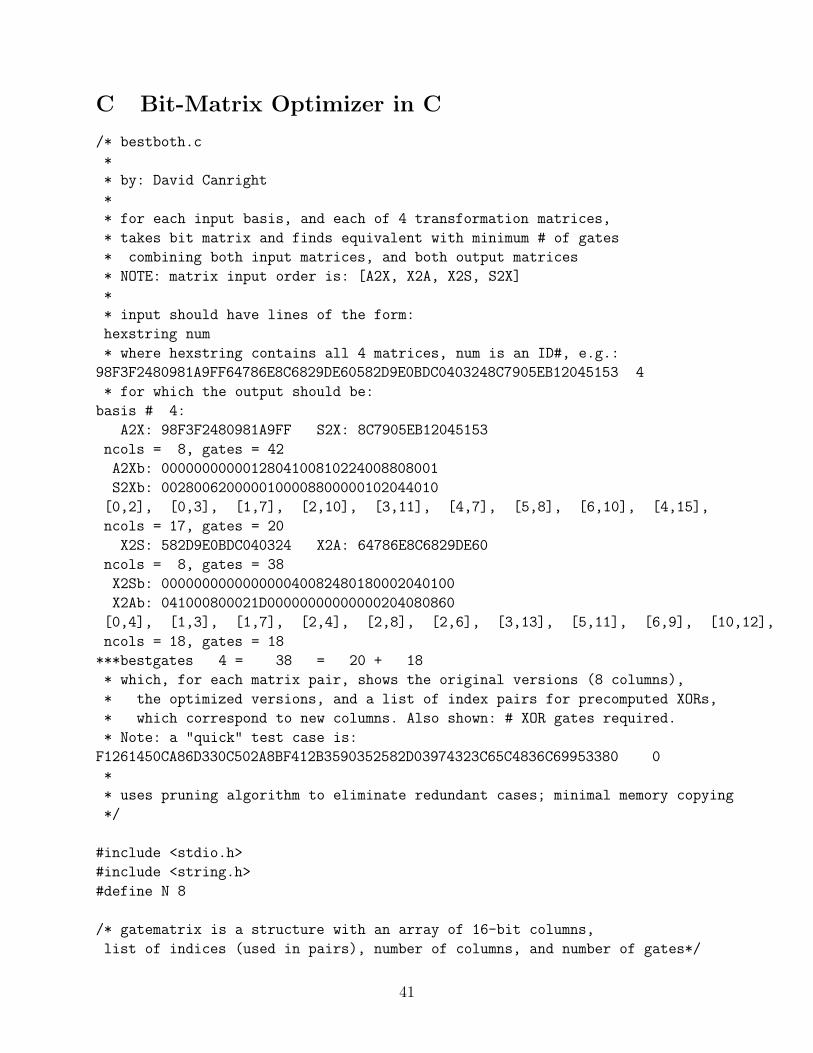
C Bit-Matrix Optimizer in C
/* bestboth.c
*
* by: David Canright
*
* for each input basis, and each of 4 transformation matrices,
* takes bit matrix and finds equivalent with minimum # of gates
* combining both input matrices, and both output matrices
* NOTE: matrix input order is: [A2X, X2A, X2S, S2X]
*
* input should have lines of the form:
hexstring num
* where hexstring contains all 4 matrices, num is an ID#, e.g.:
98F3F2480981A9FF64786E8C6829DE60582D9E0BDC0403248C7905EB12045153 4
* for which the output should be:
basis # 4:
A2X: 98F3F2480981A9FF S2X: 8C7905EB12045153
ncols = 8, gates = 42
A2Xb: 0000000000012804100810224008808001
S2Xb: 0028006200000100008800000102044010
[0,2], [0,3], [1,7], [2,10], [3,11], [4,7], [5,8], [6,10], [4,15],
ncols = 17, gates = 20
X2S: 582D9E0BDC040324 X2A: 64786E8C6829DE60
ncols = 8, gates = 38
X2Sb: 000000000000000040082480180002040100
X2Ab: 041000800021D00000000000000204080860
[0,4], [1,3], [1,7], [2,4], [2,8], [2,6], [3,13], [5,11], [6,9], [10,12],
ncols = 18, gates = 18
***bestgates 4 = 38 = 20 + 18
* which, for each matrix pair, shows the original versions (8 columns),
* the optimized versions, and a list of index pairs for precomputed XORs,
* which correspond to new columns. Also shown: # XOR gates required.
* Note: a "quick" test case is:
F1261450CA86D330C502A8BF412B3590352582D03974323C65C4836C69953380 0
*
* uses pruning algorithm to eliminate redundant cases; minimal memory copying
*/
#include <stdio.h>
#include <string.h>
#define N 8
/* gatematrix is a structure with an array of 16-bit columns,
list of indices (used in pairs), number of columns, and number of gates*/
41
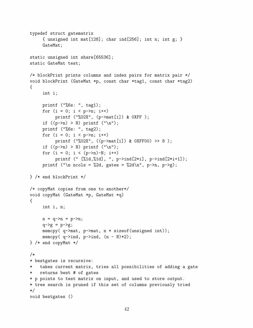
typedef struct gatematrix
unsigned int mat[128]; char ind[256]; int n; int g;
GateMat;
static unsigned int share[65536];
static GateMat test;
/* blockPrint prints columns and index pairs for matrix pair */
void blockPrint (GateMat *p, const char *tag1, const char *tag2)
int i;
printf ("%6s: ", tag1);
for (i = 0; i < p->n; i++)
printf ("%02X", (p->mat[i]) & 0XFF );
if ((p->n) > N) printf ("\n");
printf ("%6s: ", tag2);
for (i = 0; i < p->n; i++)
printf ("%02X", ((p->mat[i]) & 0XFF00) >> 8 );
if ((p->n) > N) printf ("\n");
for (i = 0; i < (p->n)-N; i++)
printf (" [%1d,%1d], ", p->ind[2*i], p->ind[2*i+1]);
printf ("\n ncols = %2d, gates = %2d\n", p->n, p->g);
/* end blockPrint */
/* copyMat copies from one to another*/
void copyMat (GateMat *p, GateMat *q)
int i, n;
n = q->n = p->n;
q->g = p->g;
memcpy( q->mat, p->mat, n * sizeof(unsigned int));
memcpy( q->ind, p->ind, (n - N)*2);
/* end copyMat */
/*
* bestgates is recursive:
* takes current matrix, tries all possibilities of adding a gate
* returns best # of gates
* p points to test matrix on input, and used to store output.
* tree search is pruned if this set of columns previously tried
*/
void bestgates ()
42

char indb[256];
int gb, nb, ci, cj;
int i, j, n, c, g, io, jo;
int nm, np, n2, n2p, t;
gb = 1024; /* best # gates, start high */
n = test.n; g = test.g;
nm=n-1; np=n+1; n2=2*(n-N); n2p=n2+1;
if (n==N) io = jo = 0; /* if orig matrix, no "old" index pair */
else io = (test.ind[n2-2]); jo = (test.ind[n2-1]);
for (i=0;i<nm;i++) /* for each pair of columns */
for (j=i+1;j<n;j++)
c = (test.mat[i]) & (test.mat[j]);
if (t=share[c]) /* if can share a gate */
if (i<io && j!=io && j!=jo && j<nm) /* if prior, indep. pair */
continue; /* then been there, done that; skip to next j */
test.n = np;
test.g = g - t;
ci = test.mat[i]; /* save current columns */
cj = test.mat[j];
test.mat[i] ^= c; /* update to new columns */
test.mat[j] ^= c;
test.mat[n] = c;
test.ind[n2] = i;
test.ind[n2p] = j;
bestgates(); /* recurse with new matrix */
test.mat[i] = ci; /* restore current columns */
test.mat[j] = cj;
if ( test.g < gb ) /* if best yet, save data */
memcpy( indb, test.ind+n2, (test.n - n)*2);
nb = test.n;
gb = test.g;
/* end columns loop */
if (gb < 1024) /* if improved, return best data */
memcpy( test.ind+n2, indb, (nb - n)*2);
test.n = nb;
test.g = gb;
/* else printf("%3d [%2d]",n,g); fflush(stdout); */
/* end bestgates */
/* bestmat reconstructs best matrix */
43
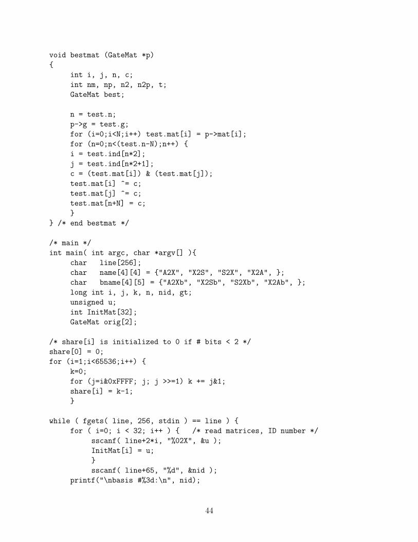
void bestmat (GateMat *p)
int i, j, n, c;
int nm, np, n2, n2p, t;
GateMat best;
n = test.n;
p->g = test.g;
for (i=0;i<N;i++) test.mat[i] = p->mat[i];
for (n=0;n<(test.n-N);n++)
i = test.ind[n*2];
j = test.ind[n*2+1];
c = (test.mat[i]) & (test.mat[j]);
test.mat[i] ^= c;
test.mat[j] ^= c;
test.mat[n+N] = c;
/* end bestmat */
/* main */
int main( int argc, char *argv[] )
char line[256];
char name[4][4] = "A2X", "X2S", "S2X", "X2A", ;
char bname[4][5] = "A2Xb", "X2Sb", "S2Xb", "X2Ab", ;
long int i, j, k, n, nid, gt;
unsigned u;
int InitMat[32];
GateMat orig[2];
/* share[i] is initialized to 0 if # bits < 2 */
share[0] = 0;
for (i=1;i<65536;i++)
k=0;
for (j=i&0xFFFF; j; j >>=1) k += j&1;
share[i] = k-1;
while ( fgets( line, 256, stdin ) == line )
for ( i=0; i < 32; i++ ) /* read matrices, ID number */
sscanf( line+2*i, "%02X", &u );
InitMat[i] = u;
sscanf( line+65, "%d", &nid );
printf("\nbasis #%3d:\n", nid);
44
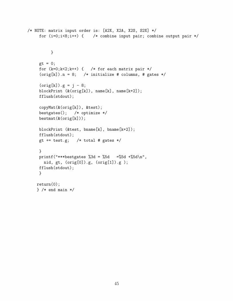
/* NOTE: matrix input order is: [A2X, X2A, X2S, S2X] */
for (i=0;i<8;i++) /* combine input pair; combine output pair */
(orig[0]).mat[i] = InitMat[8*0+i] | (InitMat[8*3+i] <<8) ;
(orig[1]).mat[i] = InitMat[8*2+i] | (InitMat[8*1+i] <<8) ;
gt = 0;
for (k=0;k<2;k++) /* for each matrix pair */
(orig[k]).n = 8; /* initialize # columns, # gates */
for (i=j=0; i<8; i++) j += share[ (orig[k]).mat[i] ];
(orig[k]).g = j - 8;
blockPrint (&(orig[k]), name[k], name[k+2]);
fflush(stdout);
copyMat(&(orig[k]), &test);
bestgates(); /* optimize */
bestmat(&(orig[k]));
blockPrint (&test, bname[k], bname[k+2]);
fflush(stdout);
gt += test.g; /* total # gates */
printf("***bestgates %3d = %5d =%5d +%5d\n",
nid, gt, (orig[0]).g, (orig[1]).g );
fflush(stdout);
return(0);
/* end main */
45

D Tables for GF(28)
D.1 Logarithm Table
For each number in decimal, hexadecimal, and binary, gives the logarithm base B in GF(28),using the polynomial basis from the root A of q(x) = x8 +x4 +x3 +x+1, where B = A+1.(See Table D.3 for an explanation of the names.)
dec hex binary logB name
0 00 00000000 −∞ 01 01 00000001 0 12 02 00000010 25 A3 03 00000011 1 B4 04 00000100 50 A2
5 05 00000101 2 B2
6 06 00000110 26 C2
7 07 00000111 198 F 64
8 08 00001000 75 E64
9 09 00001001 199 D8
10 0A 00001010 27 F11 0B 00001011 104 C8
12 0C 00001100 51 γ13 0D 00001101 238 β14 0E 00001110 223 b32
15 0F 00001111 3 K16 10 00010000 100 A4
17 11 00010001 4 B4
18 12 00010010 224 d32
19 13 00010011 14 d2
20 14 00010100 52 C4
21 15 00010101 141 F 128
22 16 00010110 129 K128
23 17 00010111 239 b16
24 18 00011000 76 g4
25 19 00011001 113 J16
26 1A 00011010 8 B8
27 1B 00011011 200 A8
28 1C 00011100 248 D29 1D 00011101 105 E8
30 1E 00011110 28 d4
31 1F 00011111 193 d64
dec hex binary logB name
32 20 00100000 125 R128
33 21 00100001 194 s64
34 22 00100010 29 j32
35 23 00100011 181 h2
36 24 00100100 249 k2
37 25 00100101 185 a64
38 26 00100110 39 f 8
39 27 00100111 106 M128
40 28 00101000 77 M16
41 29 00101001 228 f42 2A 00101010 166 M8
43 2B 00101011 114 f 128
44 2C 00101100 154 M32
45 2D 00101101 201 f 2
46 2E 00101110 9 l47 2F 00101111 120 T 8
48 30 00110000 101 m32
49 31 00110001 47 c16
50 32 00110010 138 N128
51 33 00110011 5 r52 34 00110100 33 l32
53 35 00110101 15 T54 36 00110110 225 T 32
55 37 00110111 36 l4
56 38 00111000 18 l2
57 39 00111001 240 T 16
58 3A 00111010 130 r128
59 3B 00111011 69 N64
60 3C 00111100 53 M64
61 3D 00111101 147 f 4
62 3E 00111110 218 h63 3F 00111111 142 j16
46
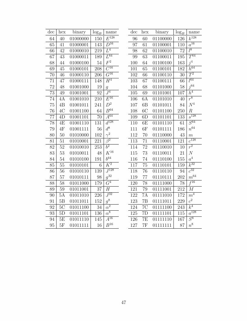
dec hex binary logB name
64 40 01000000 150 E128
65 41 01000001 143 D16
66 42 01000010 219 L4
67 43 01000011 189 L64
68 44 01000100 54 F 2
69 45 01000101 208 C16
70 46 01000110 206 G16
71 47 01000111 148 H4
72 48 01001000 19 g73 49 01001001 92 J4
74 4A 01001010 210 E16
75 4B 01001011 241 D2
76 4C 01001100 64 B64
77 4D 01001101 70 A64
78 4E 01001110 131 d128
79 4F 01001111 56 d8
80 50 01010000 102 γ2
81 51 01010001 221 β2
82 52 01010010 253 b2
83 53 01010011 48 K16
84 54 01010100 191 b64
85 55 01010101 6 K2
86 56 01010110 139 J128
87 57 01010111 98 g32
88 58 01011000 179 G4
89 59 01011001 37 H90 5A 01011010 226 J32
91 5B 01011011 152 g8
92 5C 01011100 34 α2
93 5D 01011101 136 α8
94 5E 01011110 145 A16
95 5F 01011111 16 B16
dec hex binary logB name
96 60 01100000 126 k128
97 61 01100001 110 a16
98 62 01100010 72 l8
99 63 01100011 195 T 64
100 64 01100100 163 j4
101 65 01100101 182 h64
102 66 01100110 30 T 2
103 67 01100111 66 l64
104 68 01101000 58 j64
105 69 01101001 107 h4
106 6A 01101010 40 r8
107 6B 01101011 84 N4
108 6C 01101100 250 R109 6D 01101101 133 s128
110 6E 01101110 61 S64
111 6F 01101111 186 n64
112 70 01110000 43 m113 71 01110001 121 c128
114 72 01110010 10 r2
115 73 01110011 21 N116 74 01110100 155 a4
117 75 01110101 159 k32
118 76 01110110 94 c32
119 77 01110111 202 m64
120 78 01111000 78 f 16
121 79 01111001 212 M122 7A 01111010 172 m4
123 7B 01111011 229 c2
124 7C 01111100 243 k4
125 7D 01111101 115 a128
126 7E 01111110 167 S8
127 7F 01111111 87 n8
47

dec hex binary logB name
128 80 10000000 175 R16
129 81 10000001 88 s8
130 82 10000010 168 N8
131 83 10000011 80 r16
132 84 10000100 244 S133 85 10000101 234 n134 86 10000110 214 h8
135 87 10000111 116 j128
136 88 10001000 79 S16
137 89 10001001 174 n16
138 8A 10001010 233 S2
139 8B 10001011 213 n2
140 8C 10001100 231 k8
141 8D 10001101 230 a142 8E 10001110 173 h16
143 8F 10001111 232 j144 90 10010000 44 s4
145 91 10010001 215 R8
146 92 10010010 117 n128
147 93 10010011 122 S128
148 94 10010100 235 R4
149 95 10010101 22 s2
150 96 10010110 11 s151 97 10010111 245 R2
152 98 10011000 89 m8
153 99 10011001 203 c4
154 9A 10011010 95 R32
155 9B 10011011 176 s16
156 9C 10011100 156 f 32
157 9D 10011101 169 M2
158 9E 10011110 81 N16
159 9F 10011111 160 r32
dec hex binary logB name
160 A0 10100000 127 b128
161 A1 10100001 12 K4
162 A2 10100010 246 L163 A3 10100011 111 L16
164 A4 10100100 23 J165 A5 10100101 196 g64
166 A6 10100110 73 H64
167 A7 10100111 236 G168 A8 10101000 216 F 8
169 A9 10101001 67 C64
170 AA 10101010 31 D32
171 AB 10101011 45 E172 AC 10101100 164 H32
173 AD 10101101 118 G128
174 AE 10101110 123 L128
175 AF 10101111 183 L8
176 B0 10110000 204 γ4
177 B1 10110001 187 β4
178 B2 10110010 62 D64
179 B3 10110011 90 E2
180 B4 10110100 251 b4
181 B5 10110101 96 K32
182 B6 10110110 177 F 16
183 B7 10110111 134 C128
184 B8 10111000 59 G64
185 B9 10111001 82 H16
186 BA 10111010 161 C32
187 BB 10111011 108 F 4
188 BC 10111100 170 Ω2
189 BD 10111101 85 Ω190 BE 10111110 41 H8
191 BF 10111111 157 G32
48

dec hex binary logB name
192 C0 11000000 151 c8
193 C1 11000001 178 m16
194 C2 11000010 135 T 128
195 C3 11000011 144 l16
196 C4 11000100 97 s32
197 C5 11000101 190 R64
198 C6 11000110 220 a32
199 C7 11000111 252 k200 C8 11001000 188 c64
201 C9 11001001 149 m128
202 CA 11001010 207 k16
203 CB 11001011 205 a2
204 CC 11001100 55 a8
205 CD 11001101 63 k64
206 CE 11001110 91 h32
207 CF 11001111 209 j2
208 D0 11010000 83 M4
209 D1 11010001 57 f 64
210 D2 11010010 132 l128
211 D3 11010011 60 T 4
212 D4 11010100 65 r64
213 D5 11010101 162 N32
214 D6 11010110 109 h128
215 D7 11010111 71 j8
216 D8 11011000 20 r4
217 D9 11011001 42 N2
218 DA 11011010 158 S32
219 DB 11011011 93 n32
220 DC 11011100 86 m2
221 DD 11011101 242 c222 DE 11011110 211 S4
223 DF 11011111 171 n4
dec hex binary logB name
224 E0 11100000 68 α4
225 E1 11100001 17 α226 E2 11100010 146 H128
227 E3 11100011 217 G2
228 E4 11100100 35 A32
229 E5 11100101 32 B32
230 E6 11100110 46 J2
231 E7 11100111 137 g128
232 E8 11101000 180 E4
233 E9 11101001 124 D128
234 EA 11101010 184 J8
235 EB 11101011 38 g2
236 EC 11101100 119 β8
237 ED 11101101 153 γ8
238 EE 11101110 227 D4
239 EF 11101111 165 E32
240 F0 11110000 103 G8
241 F1 11110001 74 H2
242 F2 11110010 237 L2
243 F3 11110011 222 L32
244 F4 11110100 197 J64
245 F5 11110101 49 g16
246 F6 11110110 254 b247 F7 11110111 24 K8
248 F8 11111000 13 C249 F9 11111001 99 F 32
250 FA 11111010 140 A128
251 FB 11111011 128 B128
252 FC 11111100 192 K64
253 FD 11111101 247 b8
254 FE 11111110 112 d16
255 FF 11111111 7 d
49
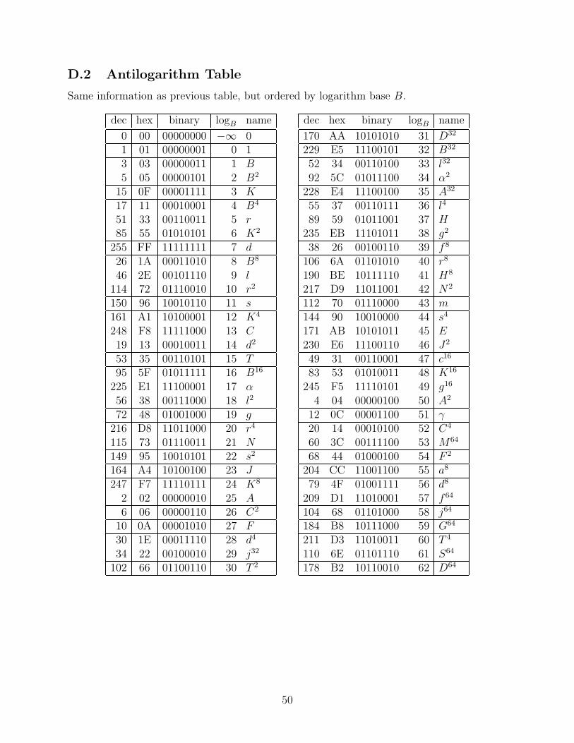
D.2 Antilogarithm Table
Same information as previous table, but ordered by logarithm base B.
dec hex binary logB name
0 00 00000000 −∞ 01 01 00000001 0 13 03 00000011 1 B5 05 00000101 2 B2
15 0F 00001111 3 K17 11 00010001 4 B4
51 33 00110011 5 r85 55 01010101 6 K2
255 FF 11111111 7 d26 1A 00011010 8 B8
46 2E 00101110 9 l114 72 01110010 10 r2
150 96 10010110 11 s161 A1 10100001 12 K4
248 F8 11111000 13 C19 13 00010011 14 d2
53 35 00110101 15 T95 5F 01011111 16 B16
225 E1 11100001 17 α56 38 00111000 18 l2
72 48 01001000 19 g216 D8 11011000 20 r4
115 73 01110011 21 N149 95 10010101 22 s2
164 A4 10100100 23 J247 F7 11110111 24 K8
2 02 00000010 25 A6 06 00000110 26 C2
10 0A 00001010 27 F30 1E 00011110 28 d4
34 22 00100010 29 j32
102 66 01100110 30 T 2
dec hex binary logB name
170 AA 10101010 31 D32
229 E5 11100101 32 B32
52 34 00110100 33 l32
92 5C 01011100 34 α2
228 E4 11100100 35 A32
55 37 00110111 36 l4
89 59 01011001 37 H235 EB 11101011 38 g2
38 26 00100110 39 f 8
106 6A 01101010 40 r8
190 BE 10111110 41 H8
217 D9 11011001 42 N2
112 70 01110000 43 m144 90 10010000 44 s4
171 AB 10101011 45 E230 E6 11100110 46 J2
49 31 00110001 47 c16
83 53 01010011 48 K16
245 F5 11110101 49 g16
4 04 00000100 50 A2
12 0C 00001100 51 γ20 14 00010100 52 C4
60 3C 00111100 53 M64
68 44 01000100 54 F 2
204 CC 11001100 55 a8
79 4F 01001111 56 d8
209 D1 11010001 57 f 64
104 68 01101000 58 j64
184 B8 10111000 59 G64
211 D3 11010011 60 T 4
110 6E 01101110 61 S64
178 B2 10110010 62 D64
50
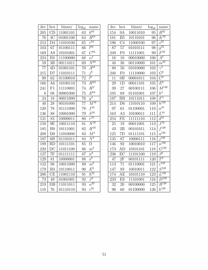
dec hex binary logB name
205 CD 11001101 63 k64
76 4C 01001100 64 B64
212 D4 11010100 65 r64
103 67 01100111 66 l64
169 A9 10101001 67 C64
224 E0 11100000 68 α4
59 3B 00111011 69 N64
77 4D 01001101 70 A64
215 D7 11010111 71 j8
98 62 01100010 72 l8
166 A6 10100110 73 H64
241 F1 11110001 74 H2
8 08 00001000 75 E64
24 18 00011000 76 g4
40 28 00101000 77 M16
120 78 01111000 78 f 16
136 88 10001000 79 S16
131 83 10000011 80 r16
158 9E 10011110 81 N16
185 B9 10111001 82 H16
208 D0 11010000 83 M4
107 6B 01101011 84 N4
189 BD 10111101 85 Ω220 DC 11011100 86 m2
127 7F 01111111 87 n8
129 81 10000001 88 s8
152 98 10011000 89 m8
179 B3 10110011 90 E2
206 CE 11001110 91 h32
73 49 01001001 92 J4
219 DB 11011011 93 n32
118 76 01110110 94 c32
dec hex binary logB name
154 9A 10011010 95 R32
181 B5 10110101 96 K32
196 C4 11000100 97 s32
87 57 01010111 98 g32
249 F9 11111001 99 F 32
16 10 00010000 100 A4
48 30 00110000 101 m32
80 50 01010000 102 γ2
240 F0 11110000 103 G8
11 0B 00001011 104 C8
29 1D 00011101 105 E8
39 27 00100111 106 M128
105 69 01101001 107 h4
187 BB 10111011 108 F 4
214 D6 11010110 109 h128
97 61 01100001 110 a16
163 A3 10100011 111 L16
254 FE 11111110 112 d16
25 19 00011001 113 J16
43 2B 00101011 114 f 128
125 7D 01111101 115 a128
135 87 10000111 116 j128
146 92 10010010 117 n128
173 AD 10101101 118 G128
236 EC 11101100 119 β8
47 2F 00101111 120 T 8
113 71 01110001 121 c128
147 93 10010011 122 S128
174 AE 10101110 123 L128
233 E9 11101001 124 D128
32 20 00100000 125 R128
96 60 01100000 126 k128
51

dec hex binary logB name
160 A0 10100000 127 b128
251 FB 11111011 128 B128
22 16 00010110 129 K128
58 3A 00111010 130 r128
78 4E 01001110 131 d128
210 D2 11010010 132 l128
109 6D 01101101 133 s128
183 B7 10110111 134 C128
194 C2 11000010 135 T 128
93 5D 01011101 136 α8
231 E7 11100111 137 g128
50 32 00110010 138 N128
86 56 01010110 139 J128
250 FA 11111010 140 A128
21 15 00010101 141 F 128
63 3F 00111111 142 j16
65 41 01000001 143 D16
195 C3 11000011 144 l16
94 5E 01011110 145 A16
226 E2 11100010 146 H128
61 3D 00111101 147 f 4
71 47 01000111 148 H4
201 C9 11001001 149 m128
64 40 01000000 150 E128
192 C0 11000000 151 c8
91 5B 01011011 152 g8
237 ED 11101101 153 γ8
44 2C 00101100 154 M32
116 74 01110100 155 a4
156 9C 10011100 156 f 32
191 BF 10111111 157 G32
218 DA 11011010 158 S32
dec hex binary logB name
117 75 01110101 159 k32
159 9F 10011111 160 r32
186 BA 10111010 161 C32
213 D5 11010101 162 N32
100 64 01100100 163 j4
172 AC 10101100 164 H32
239 EF 11101111 165 E32
42 2A 00101010 166 M8
126 7E 01111110 167 S8
130 82 10000010 168 N8
157 9D 10011101 169 M2
188 BC 10111100 170 Ω2
223 DF 11011111 171 n4
122 7A 01111010 172 m4
142 8E 10001110 173 h16
137 89 10001001 174 n16
128 80 10000000 175 R16
155 9B 10011011 176 s16
182 B6 10110110 177 F 16
193 C1 11000001 178 m16
88 58 01011000 179 G4
232 E8 11101000 180 E4
35 23 00100011 181 h2
101 65 01100101 182 h64
175 AF 10101111 183 L8
234 EA 11101010 184 J8
37 25 00100101 185 a64
111 6F 01101111 186 n64
177 B1 10110001 187 β4
200 C8 11001000 188 c64
67 43 01000011 189 L64
197 C5 11000101 190 R64
52
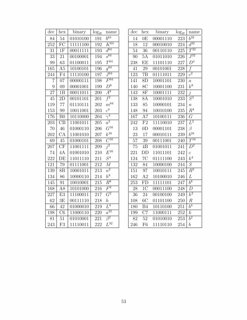
dec hex binary logB name
84 54 01010100 191 b64
252 FC 11111100 192 K64
31 1F 00011111 193 d64
33 21 00100001 194 s64
99 63 01100011 195 T 64
165 A5 10100101 196 g64
244 F4 11110100 197 J64
7 07 00000111 198 F 64
9 09 00001001 199 D8
27 1B 00011011 200 A8
45 2D 00101101 201 f 2
119 77 01110111 202 m64
153 99 10011001 203 c4
176 B0 10110000 204 γ4
203 CB 11001011 205 a2
70 46 01000110 206 G16
202 CA 11001010 207 k16
69 45 01000101 208 C16
207 CF 11001111 209 j2
74 4A 01001010 210 E16
222 DE 11011110 211 S4
121 79 01111001 212 M139 8B 10001011 213 n2
134 86 10000110 214 h8
145 91 10010001 215 R8
168 A8 10101000 216 F 8
227 E3 11100011 217 G2
62 3E 00111110 218 h66 42 01000010 219 L4
198 C6 11000110 220 a32
81 51 01010001 221 β2
243 F3 11110011 222 L32
dec hex binary logB name
14 0E 00001110 223 b32
18 12 00010010 224 d32
54 36 00110110 225 T 32
90 5A 01011010 226 J32
238 EE 11101110 227 D4
41 29 00101001 228 f123 7B 01111011 229 c2
141 8D 10001101 230 a140 8C 10001100 231 k8
143 8F 10001111 232 j138 8A 10001010 233 S2
133 85 10000101 234 n148 94 10010100 235 R4
167 A7 10100111 236 G242 F2 11110010 237 L2
13 0D 00001101 238 β23 17 00010111 239 b16
57 39 00111001 240 T 16
75 4B 01001011 241 D2
221 DD 11011101 242 c124 7C 01111100 243 k4
132 84 10000100 244 S151 97 10010111 245 R2
162 A2 10100010 246 L253 FD 11111101 247 b8
28 1C 00011100 248 D36 24 00100100 249 k2
108 6C 01101100 250 R180 B4 10110100 251 b4
199 C7 11000111 252 k82 52 01010010 253 b2
246 F6 11110110 254 b
53

D.3 Polynomial Table
Each minimal polynomial over GF(2) is listed as a bit string of coefficients, e.g., 100011011means x8 + x4 + x3 + x + 1 = q(x). Reversing the bit string corresponds to inverting theroots; the ordering is in such pairs. The conjugate roots are given in terms of logB; the firstlisted is given the name shown. The “order” is in the multiplicative subgroup, e.g., γ5 = 1.
name polynomial order logB of conjugates
0 10 1 −∞1 11 1 0
Ω 111 3 85 170
α 10011 15 17 34 68 136β 11001 15 238 221 187 119γ 11111 5 51 102 204 153
A 100011011 51 25 50 100 200 145 35 70 140a 110110001 51 230 205 155 55 110 220 185 115B 100011101 255 1 2 4 8 16 32 64 128b 101110001 255 254 253 251 247 239 223 191 127C 100101011 255 13 26 52 104 208 161 67 134c 110101001 255 242 229 203 151 47 94 188 121D 100101101 255 248 241 227 199 143 31 62 124d 101101001 255 7 14 28 56 112 224 193 131E 100111001 17 45 90 180 105 210 165 75 150F 100111111 85 27 54 108 216 177 99 198 141f 111111001 85 228 201 147 39 78 156 57 114G 101001101 255 236 217 179 103 206 157 59 118g 101100101 255 19 38 76 152 49 98 196 137H 101011111 255 37 74 148 41 82 164 73 146h 111110101 255 218 181 107 214 173 91 182 109J 101100011 255 23 46 92 184 113 226 197 139j 110001101 255 232 209 163 71 142 29 58 116K 101110111 85 3 6 12 24 48 96 192 129k 111011101 85 252 249 243 231 207 159 63 126L 101111011 85 246 237 219 183 111 222 189 123l 110111101 85 9 18 36 72 144 33 66 132
M 110000111 255 212 169 83 166 77 154 53 106m 111000011 255 43 86 172 89 178 101 202 149N 110001011 85 21 42 84 168 81 162 69 138n 110100011 85 234 213 171 87 174 93 186 117R 110011111 51 250 245 235 215 175 95 190 125r 111110011 51 5 10 20 40 80 160 65 130S 111001111 255 244 233 211 167 79 158 61 122s 111100111 255 11 22 44 88 176 97 194 133T 111010111 17 15 30 60 120 240 225 195 135
54

E All Possible Bases
The following table shows all 432 possible combinations of bases for GF(28), GF(24), andGF(22) for which the trace is unity (τ = T = 1). Each subfield basis is given as an orderedpair; if the second entry is 1 then it is a polynomial basis, otherwise a normal basis. TheGF(28) basis uses roots of r(y) = y2 +y+ν, the GF(24) basis uses roots of s(z) = z2 +z+N ,where ν and N are the respective norms, and the GF(22) basis uses roots of t(w) = w2+w+1.
The basis and norm entries use the naming convention summarized in Table D.3. Ex-plicitly, in terms of the standard AES basis: in subfield GF(22), Ω = 189 = 0xBD; insubfield GF(24), α = 225 = 0xE1, β = 13 = 0x0D, and γ = 12 = 0x0C; in the main field,d = 255 = 0xFF and L = 162 = 0xA2.
The coefficients C and D of ν with respect to the GF(24) basis are given in terms of N ,as is the root w, as on page 18.
Under “XOR Gates,” the first column shows the number of XOR gates for the inverter;each also includes 36 AND’s. For bases 1–144, this number includes all of the low-leveloptimizations given in Section 4.4; bases 145 and beyond use a polynomial basis for GF(28),and for those cases the inverter number is an estimate (except for 8 cases where theseoptimizations were explicitly included: 159, 177, 191, 209, 234, 252, 260, and 278). Thelast three columns show the XOR’s for a complete S-box, an inverse S-box, and a mergedcombination of both with a shared inverter (excluding multiplexors); each would also have36 AND’s and possibly a few NOT’s (for the affine transformation). A superscript o in thelast column means the 16 × 8 basis change matrices were fully optimized by the tree-searchalgorithm; otherwise they were factored by the greedy algorithm. (All of the 8× 8 matriceswere fully optimized.)
55

Case Bases Norms Coefficients XOR Gates# GF(28) GF(24) GF(22) ν N C D w = inv. S-box S-box−1 Both
1 [d16, d] [α4, α] [Ω2, Ω] β8 Ω N2 1 N 66 99 94 1222 [d16, d] [α4, α] [Ω, 1] β8 Ω N2 1 N 66 94 93 1193 [d16, d] [α4, α] [Ω2, 1] β8 Ω N2 1 N2 66 94 92 1164 [d16, d] [α8, α2] [Ω2, Ω] β8 Ω2 0 N2 N2 66 90 91 104o
5 [d16, d] [α8, α2] [Ω, 1] β8 Ω2 0 N2 N2 66 92 92 109o
6 [d16, d] [α8, α2] [Ω2, 1] β8 Ω2 0 N2 N 66 92 94 112o
7 [d16, d] [α, 1] [Ω2, Ω] β8 Ω N N2 N 67 97 94 1198 [d16, d] [α, 1] [Ω, 1] β8 Ω N N2 N 68 95 95 1179 [d16, d] [α, 1] [Ω2, 1] β8 Ω N N2 N2 68 98 94 119
10 [d16, d] [α4, 1] [Ω2, Ω] β8 Ω N 1 N 67 95 94 11711 [d16, d] [α4, 1] [Ω, 1] β8 Ω N 1 N 67 93 94 11512 [d16, d] [α4, 1] [Ω2, 1] β8 Ω N 1 N2 67 94 94 11813 [d16, d] [α2, 1] [Ω2, Ω] β8 Ω2 N2 0 N2 67 91 92 11414 [d16, d] [α2, 1] [Ω, 1] β8 Ω2 N2 0 N2 67 93 93 11415 [d16, d] [α2, 1] [Ω2, 1] β8 Ω2 N2 0 N 67 94 95 11816 [d16, d] [α8, 1] [Ω2, Ω] β8 Ω2 N2 N2 N2 67 91 93 111o
17 [d16, d] [α8, 1] [Ω, 1] β8 Ω2 N2 N2 N2 67 92 94 112o
18 [d16, d] [α8, 1] [Ω2, 1] β8 Ω2 N2 N2 N 67 93 94 11719 [d32, d2] [α4, α] [Ω2, Ω] β Ω N2 0 N 66 96 98 12420 [d32, d2] [α4, α] [Ω, 1] β Ω N2 0 N 66 97 99 11821 [d32, d2] [α4, α] [Ω2, 1] β Ω N2 0 N2 66 95 97 11622 [d32, d2] [α8, α2] [Ω2, Ω] β Ω2 N2 1 N2 66 96 97 11623 [d32, d2] [α8, α2] [Ω, 1] β Ω2 N2 1 N2 66 94 92 107o
24 [d32, d2] [α8, α2] [Ω2, 1] β Ω2 N2 1 N 66 94 94 11725 [d32, d2] [α, 1] [Ω2, Ω] β Ω N2 N2 N 67 97 98 12126 [d32, d2] [α, 1] [Ω, 1] β Ω N2 N2 N 67 96 97 12227 [d32, d2] [α, 1] [Ω2, 1] β Ω N2 N2 N2 67 97 95 12128 [d32, d2] [α4, 1] [Ω2, Ω] β Ω N2 0 N 67 97 98 12229 [d32, d2] [α4, 1] [Ω, 1] β Ω N2 0 N 67 96 93 11730 [d32, d2] [α4, 1] [Ω2, 1] β Ω N2 0 N2 67 96 97 11831 [d32, d2] [α2, 1] [Ω2, Ω] β Ω2 N N2 N2 67 96 97 12232 [d32, d2] [α2, 1] [Ω, 1] β Ω2 N N2 N2 68 98 94 11533 [d32, d2] [α2, 1] [Ω2, 1] β Ω2 N N2 N 68 99 96 12034 [d32, d2] [α8, 1] [Ω2, Ω] β Ω2 N 1 N2 67 94 97 112o
35 [d32, d2] [α8, 1] [Ω, 1] β Ω2 N 1 N2 67 93 93 110o
36 [d32, d2] [α8, 1] [Ω2, 1] β Ω2 N 1 N 67 92 94 118
ofully optimized results
56
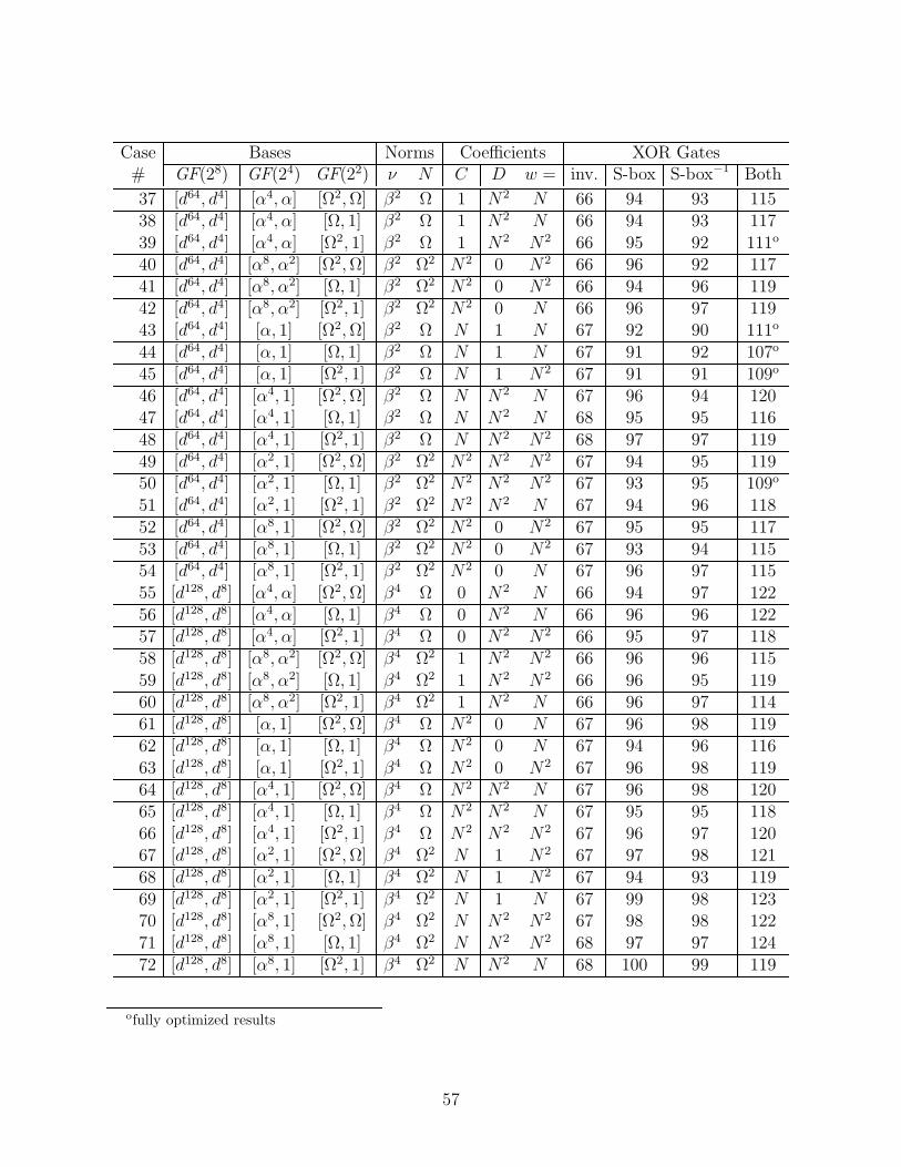
Case Bases Norms Coefficients XOR Gates# GF(28) GF(24) GF(22) ν N C D w = inv. S-box S-box−1 Both
37 [d64, d4] [α4, α] [Ω2, Ω] β2 Ω 1 N2 N 66 94 93 11538 [d64, d4] [α4, α] [Ω, 1] β2 Ω 1 N2 N 66 94 93 11739 [d64, d4] [α4, α] [Ω2, 1] β2 Ω 1 N2 N2 66 95 92 111o
40 [d64, d4] [α8, α2] [Ω2, Ω] β2 Ω2 N2 0 N2 66 96 92 11741 [d64, d4] [α8, α2] [Ω, 1] β2 Ω2 N2 0 N2 66 94 96 11942 [d64, d4] [α8, α2] [Ω2, 1] β2 Ω2 N2 0 N 66 96 97 11943 [d64, d4] [α, 1] [Ω2, Ω] β2 Ω N 1 N 67 92 90 111o
44 [d64, d4] [α, 1] [Ω, 1] β2 Ω N 1 N 67 91 92 107o
45 [d64, d4] [α, 1] [Ω2, 1] β2 Ω N 1 N2 67 91 91 109o
46 [d64, d4] [α4, 1] [Ω2, Ω] β2 Ω N N2 N 67 96 94 12047 [d64, d4] [α4, 1] [Ω, 1] β2 Ω N N2 N 68 95 95 11648 [d64, d4] [α4, 1] [Ω2, 1] β2 Ω N N2 N2 68 97 97 11949 [d64, d4] [α2, 1] [Ω2, Ω] β2 Ω2 N2 N2 N2 67 94 95 11950 [d64, d4] [α2, 1] [Ω, 1] β2 Ω2 N2 N2 N2 67 93 95 109o
51 [d64, d4] [α2, 1] [Ω2, 1] β2 Ω2 N2 N2 N 67 94 96 11852 [d64, d4] [α8, 1] [Ω2, Ω] β2 Ω2 N2 0 N2 67 95 95 11753 [d64, d4] [α8, 1] [Ω, 1] β2 Ω2 N2 0 N2 67 93 94 11554 [d64, d4] [α8, 1] [Ω2, 1] β2 Ω2 N2 0 N 67 96 97 11555 [d128, d8] [α4, α] [Ω2, Ω] β4 Ω 0 N2 N 66 94 97 12256 [d128, d8] [α4, α] [Ω, 1] β4 Ω 0 N2 N 66 96 96 12257 [d128, d8] [α4, α] [Ω2, 1] β4 Ω 0 N2 N2 66 95 97 11858 [d128, d8] [α8, α2] [Ω2, Ω] β4 Ω2 1 N2 N2 66 96 96 11559 [d128, d8] [α8, α2] [Ω, 1] β4 Ω2 1 N2 N2 66 96 95 11960 [d128, d8] [α8, α2] [Ω2, 1] β4 Ω2 1 N2 N 66 96 97 11461 [d128, d8] [α, 1] [Ω2, Ω] β4 Ω N2 0 N 67 96 98 11962 [d128, d8] [α, 1] [Ω, 1] β4 Ω N2 0 N 67 94 96 11663 [d128, d8] [α, 1] [Ω2, 1] β4 Ω N2 0 N2 67 96 98 11964 [d128, d8] [α4, 1] [Ω2, Ω] β4 Ω N2 N2 N 67 96 98 12065 [d128, d8] [α4, 1] [Ω, 1] β4 Ω N2 N2 N 67 95 95 11866 [d128, d8] [α4, 1] [Ω2, 1] β4 Ω N2 N2 N2 67 96 97 12067 [d128, d8] [α2, 1] [Ω2, Ω] β4 Ω2 N 1 N2 67 97 98 12168 [d128, d8] [α2, 1] [Ω, 1] β4 Ω2 N 1 N2 67 94 93 11969 [d128, d8] [α2, 1] [Ω2, 1] β4 Ω2 N 1 N 67 99 98 12370 [d128, d8] [α8, 1] [Ω2, Ω] β4 Ω2 N N2 N2 67 98 98 12271 [d128, d8] [α8, 1] [Ω, 1] β4 Ω2 N N2 N2 68 97 97 12472 [d128, d8] [α8, 1] [Ω2, 1] β4 Ω2 N N2 N 68 100 99 119
ofully optimized results
57

Case Bases Norms Coefficients XOR Gates# GF(28) GF(24) GF(22) ν N C D w = inv. S-box S-box−1 Both
73 [L16, L] [α4, α] [Ω2, Ω] γ2 Ω 0 N N 66 94 93 11774 [L16, L] [α4, α] [Ω, 1] γ2 Ω 0 N N 66 96 95 12075 [L16, L] [α4, α] [Ω2, 1] γ2 Ω 0 N N2 66 96 93 11976 [L16, L] [α8, α2] [Ω2, Ω] γ2 Ω2 N 1 N2 66 92 93 11577 [L16, L] [α8, α2] [Ω, 1] γ2 Ω2 N 1 N2 66 93 94 11978 [L16, L] [α8, α2] [Ω2, 1] γ2 Ω2 N 1 N 66 93 95 11779 [L16, L] [α, 1] [Ω2, Ω] γ2 Ω N 0 N 67 93 92 11480 [L16, L] [α, 1] [Ω, 1] γ2 Ω N 0 N 67 92 93 11681 [L16, L] [α, 1] [Ω2, 1] γ2 Ω N 0 N2 67 94 93 11582 [L16, L] [α4, 1] [Ω2, Ω] γ2 Ω N N N 67 94 96 11683 [L16, L] [α4, 1] [Ω, 1] γ2 Ω N N N 67 94 93 11684 [L16, L] [α4, 1] [Ω2, 1] γ2 Ω N N N2 67 93 94 11585 [L16, L] [α2, 1] [Ω2, Ω] γ2 Ω2 N2 N N2 67 92 93 111o
86 [L16, L] [α2, 1] [Ω, 1] γ2 Ω2 N2 N N2 67 92 94 11687 [L16, L] [α2, 1] [Ω2, 1] γ2 Ω2 N2 N N 67 93 95 11788 [L16, L] [α8, 1] [Ω2, Ω] γ2 Ω2 N2 1 N2 67 94 94 11189 [L16, L] [α8, 1] [Ω, 1] γ2 Ω2 N2 1 N2 68 92 92 11590 [L16, L] [α8, 1] [Ω2, 1] γ2 Ω2 N2 1 N 67 93 93 11591 [L32, L2] [α4, α] [Ω2, Ω] γ4 Ω 1 N N 66 96 95 11992 [L32, L2] [α4, α] [Ω, 1] γ4 Ω 1 N N 66 95 96 12193 [L32, L2] [α4, α] [Ω2, 1] γ4 Ω 1 N N2 66 97 97 11894 [L32, L2] [α8, α2] [Ω2, Ω] γ4 Ω2 0 N N2 66 94 94 112o
95 [L32, L2] [α8, α2] [Ω, 1] γ4 Ω2 0 N N2 66 93 96 11896 [L32, L2] [α8, α2] [Ω2, 1] γ4 Ω2 0 N N 66 93 95 11997 [L32, L2] [α, 1] [Ω2, Ω] γ4 Ω N2 1 N 67 98 99 12598 [L32, L2] [α, 1] [Ω, 1] γ4 Ω N2 1 N 67 97 98 12499 [L32, L2] [α, 1] [Ω2, 1] γ4 Ω N2 1 N2 68 98 99 122
100 [L32, L2] [α4, 1] [Ω2, Ω] γ4 Ω N2 N N 67 92 93 117101 [L32, L2] [α4, 1] [Ω, 1] γ4 Ω N2 N N 67 96 96 120102 [L32, L2] [α4, 1] [Ω2, 1] γ4 Ω N2 N N2 67 97 97 122103 [L32, L2] [α2, 1] [Ω2, Ω] γ4 Ω2 N 0 N2 67 95 97 121104 [L32, L2] [α2, 1] [Ω, 1] γ4 Ω2 N 0 N2 67 94 96 118105 [L32, L2] [α2, 1] [Ω2, 1] γ4 Ω2 N 0 N 67 95 96 119106 [L32, L2] [α8, 1] [Ω2, Ω] γ4 Ω2 N N N2 67 95 98 121107 [L32, L2] [α8, 1] [Ω, 1] γ4 Ω2 N N N2 67 96 95 116108 [L32, L2] [α8, 1] [Ω2, 1] γ4 Ω2 N N N 67 97 97 118
ofully optimized results
58

Case Bases Norms Coefficients XOR Gates# GF(28) GF(24) GF(22) ν N C D w = inv. S-box S-box−1 Both
109 [L64, L4] [α4, α] [Ω2, Ω] γ8 Ω N 0 N 66 91 93 114110 [L64, L4] [α4, α] [Ω, 1] γ8 Ω N 0 N 66 91 92 108o
111 [L64, L4] [α4, α] [Ω2, 1] γ8 Ω N 0 N2 66 91 93 108o
112 [L64, L4] [α8, α2] [Ω2, Ω] γ8 Ω2 1 N N2 66 93 90 114113 [L64, L4] [α8, α2] [Ω, 1] γ8 Ω2 1 N N2 66 94 90 109o
114 [L64, L4] [α8, α2] [Ω2, 1] γ8 Ω2 1 N N 66 91 90 108o
115 [L64, L4] [α, 1] [Ω2, Ω] γ8 Ω N N N 67 94 96 115116 [L64, L4] [α, 1] [Ω, 1] γ8 Ω N N N 67 93 94 115117 [L64, L4] [α, 1] [Ω2, 1] γ8 Ω N N N2 67 92 94 109o
118 [L64, L4] [α4, 1] [Ω2, Ω] γ8 Ω N 0 N 67 91 94 112o
119 [L64, L4] [α4, 1] [Ω, 1] γ8 Ω N 0 N 67 93 93 118120 [L64, L4] [α4, 1] [Ω2, 1] γ8 Ω N 0 N2 67 92 93 116121 [L64, L4] [α2, 1] [Ω2, Ω] γ8 Ω2 N2 1 N2 67 96 93 119122 [L64, L4] [α2, 1] [Ω, 1] γ8 Ω2 N2 1 N2 68 95 93 114123 [L64, L4] [α2, 1] [Ω2, 1] γ8 Ω2 N2 1 N 67 95 93 116124 [L64, L4] [α8, 1] [Ω2, Ω] γ8 Ω2 N2 N N2 67 95 92 115125 [L64, L4] [α8, 1] [Ω, 1] γ8 Ω2 N2 N N2 67 93 90 110o
126 [L64, L4] [α8, 1] [Ω2, 1] γ8 Ω2 N2 N N 67 94 92 116127 [L128, L8] [α4, α] [Ω2, Ω] γ Ω N 1 N 66 96 97 119128 [L128, L8] [α4, α] [Ω, 1] γ Ω N 1 N 66 97 97 119129 [L128, L8] [α4, α] [Ω2, 1] γ Ω N 1 N2 66 98 98 121130 [L128, L8] [α8, α2] [Ω2, Ω] γ Ω2 N 0 N2 66 92 91 115131 [L128, L8] [α8, α2] [Ω, 1] γ Ω2 N 0 N2 66 94 95 120132 [L128, L8] [α8, α2] [Ω2, 1] γ Ω2 N 0 N 66 92 95 116133 [L128, L8] [α, 1] [Ω2, Ω] γ Ω N2 N N 67 98 97 120134 [L128, L8] [α, 1] [Ω, 1] γ Ω N2 N N 67 98 99 119135 [L128, L8] [α, 1] [Ω2, 1] γ Ω N2 N N2 67 97 100 121136 [L128, L8] [α4, 1] [Ω2, Ω] γ Ω N2 1 N 67 99 99 123137 [L128, L8] [α4, 1] [Ω, 1] γ Ω N2 1 N 67 96 99 122138 [L128, L8] [α4, 1] [Ω2, 1] γ Ω N2 1 N2 68 98 99 126139 [L128, L8] [α2, 1] [Ω2, Ω] γ Ω2 N N N2 67 96 99 119140 [L128, L8] [α2, 1] [Ω, 1] γ Ω2 N N N2 67 96 98 120141 [L128, L8] [α2, 1] [Ω2, 1] γ Ω2 N N N 67 96 99 122142 [L128, L8] [α8, 1] [Ω2, Ω] γ Ω2 N 0 N2 67 95 94 116143 [L128, L8] [α8, 1] [Ω, 1] γ Ω2 N 0 N2 67 95 97 119144 [L128, L8] [α8, 1] [Ω2, 1] γ Ω2 N 0 N 67 95 97 117
ofully optimized results
59
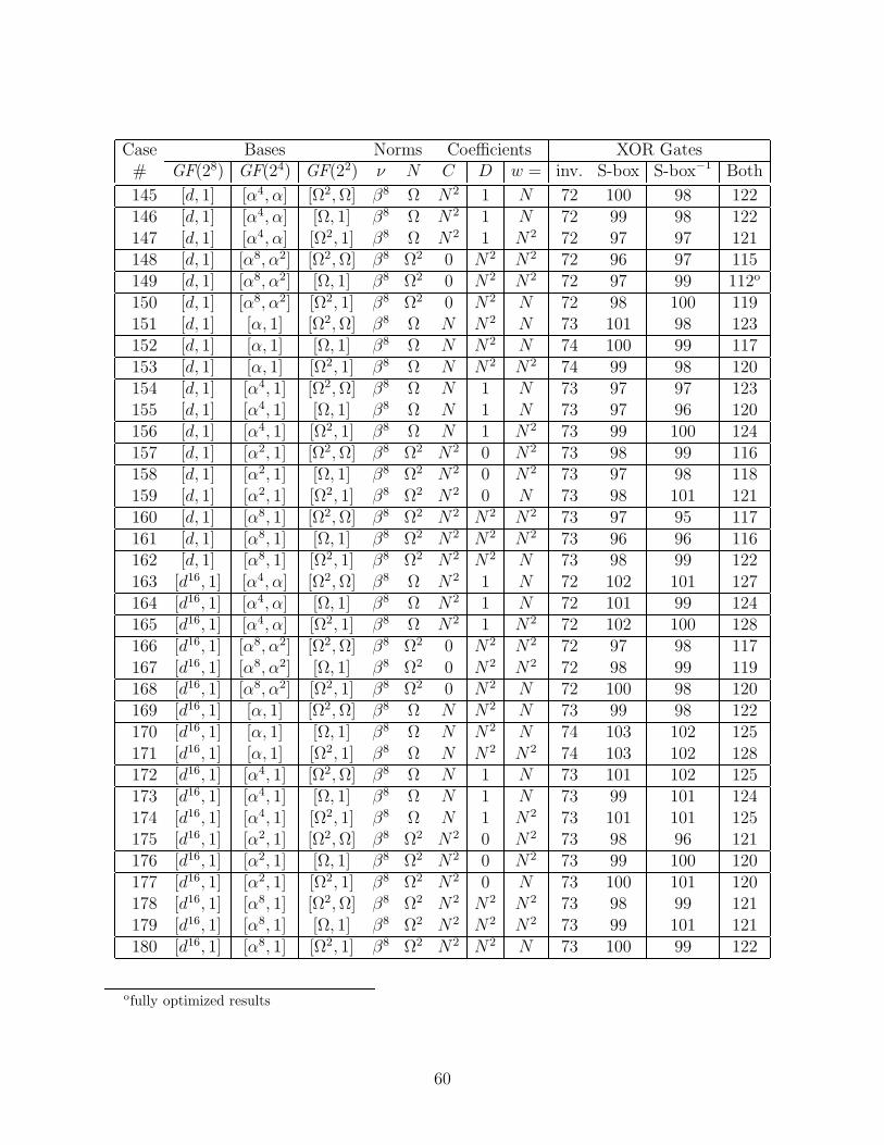
Case Bases Norms Coefficients XOR Gates# GF(28) GF(24) GF(22) ν N C D w = inv. S-box S-box−1 Both
145 [d, 1] [α4, α] [Ω2, Ω] β8 Ω N2 1 N 72 100 98 122146 [d, 1] [α4, α] [Ω, 1] β8 Ω N2 1 N 72 99 98 122147 [d, 1] [α4, α] [Ω2, 1] β8 Ω N2 1 N2 72 97 97 121148 [d, 1] [α8, α2] [Ω2, Ω] β8 Ω2 0 N2 N2 72 96 97 115149 [d, 1] [α8, α2] [Ω, 1] β8 Ω2 0 N2 N2 72 97 99 112o
150 [d, 1] [α8, α2] [Ω2, 1] β8 Ω2 0 N2 N 72 98 100 119151 [d, 1] [α, 1] [Ω2, Ω] β8 Ω N N2 N 73 101 98 123152 [d, 1] [α, 1] [Ω, 1] β8 Ω N N2 N 74 100 99 117153 [d, 1] [α, 1] [Ω2, 1] β8 Ω N N2 N2 74 99 98 120154 [d, 1] [α4, 1] [Ω2, Ω] β8 Ω N 1 N 73 97 97 123155 [d, 1] [α4, 1] [Ω, 1] β8 Ω N 1 N 73 97 96 120156 [d, 1] [α4, 1] [Ω2, 1] β8 Ω N 1 N2 73 99 100 124157 [d, 1] [α2, 1] [Ω2, Ω] β8 Ω2 N2 0 N2 73 98 99 116158 [d, 1] [α2, 1] [Ω, 1] β8 Ω2 N2 0 N2 73 97 98 118159 [d, 1] [α2, 1] [Ω2, 1] β8 Ω2 N2 0 N 73 98 101 121160 [d, 1] [α8, 1] [Ω2, Ω] β8 Ω2 N2 N2 N2 73 97 95 117161 [d, 1] [α8, 1] [Ω, 1] β8 Ω2 N2 N2 N2 73 96 96 116162 [d, 1] [α8, 1] [Ω2, 1] β8 Ω2 N2 N2 N 73 98 99 122163 [d16, 1] [α4, α] [Ω2, Ω] β8 Ω N2 1 N 72 102 101 127164 [d16, 1] [α4, α] [Ω, 1] β8 Ω N2 1 N 72 101 99 124165 [d16, 1] [α4, α] [Ω2, 1] β8 Ω N2 1 N2 72 102 100 128166 [d16, 1] [α8, α2] [Ω2, Ω] β8 Ω2 0 N2 N2 72 97 98 117167 [d16, 1] [α8, α2] [Ω, 1] β8 Ω2 0 N2 N2 72 98 99 119168 [d16, 1] [α8, α2] [Ω2, 1] β8 Ω2 0 N2 N 72 100 98 120169 [d16, 1] [α, 1] [Ω2, Ω] β8 Ω N N2 N 73 99 98 122170 [d16, 1] [α, 1] [Ω, 1] β8 Ω N N2 N 74 103 102 125171 [d16, 1] [α, 1] [Ω2, 1] β8 Ω N N2 N2 74 103 102 128172 [d16, 1] [α4, 1] [Ω2, Ω] β8 Ω N 1 N 73 101 102 125173 [d16, 1] [α4, 1] [Ω, 1] β8 Ω N 1 N 73 99 101 124174 [d16, 1] [α4, 1] [Ω2, 1] β8 Ω N 1 N2 73 101 101 125175 [d16, 1] [α2, 1] [Ω2, Ω] β8 Ω2 N2 0 N2 73 98 96 121176 [d16, 1] [α2, 1] [Ω, 1] β8 Ω2 N2 0 N2 73 99 100 120177 [d16, 1] [α2, 1] [Ω2, 1] β8 Ω2 N2 0 N 73 100 101 120178 [d16, 1] [α8, 1] [Ω2, Ω] β8 Ω2 N2 N2 N2 73 98 99 121179 [d16, 1] [α8, 1] [Ω, 1] β8 Ω2 N2 N2 N2 73 99 101 121180 [d16, 1] [α8, 1] [Ω2, 1] β8 Ω2 N2 N2 N 73 100 99 122
ofully optimized results
60

Case Bases Norms Coefficients XOR Gates# GF(28) GF(24) GF(22) ν N C D w = inv. S-box S-box−1 Both
181 [d2, 1] [α4, α] [Ω2, Ω] β Ω N2 0 N 72 100 101 124182 [d2, 1] [α4, α] [Ω, 1] β Ω N2 0 N 72 102 101 124183 [d2, 1] [α4, α] [Ω2, 1] β Ω N2 0 N2 72 99 100 121184 [d2, 1] [α8, α2] [Ω2, Ω] β Ω2 N2 1 N2 72 97 99 120185 [d2, 1] [α8, α2] [Ω, 1] β Ω2 N2 1 N2 72 98 98 116186 [d2, 1] [α8, α2] [Ω2, 1] β Ω2 N2 1 N 72 96 99 119187 [d2, 1] [α, 1] [Ω2, Ω] β Ω N2 N2 N 73 102 103 125188 [d2, 1] [α, 1] [Ω, 1] β Ω N2 N2 N 73 101 100 122189 [d2, 1] [α, 1] [Ω2, 1] β Ω N2 N2 N2 73 100 102 125190 [d2, 1] [α4, 1] [Ω2, Ω] β Ω N2 0 N 73 100 104 124191 [d2, 1] [α4, 1] [Ω, 1] β Ω N2 0 N 73 101 101 126192 [d2, 1] [α4, 1] [Ω2, 1] β Ω N2 0 N2 73 102 103 126193 [d2, 1] [α2, 1] [Ω2, Ω] β Ω2 N N2 N2 73 101 102 123194 [d2, 1] [α2, 1] [Ω, 1] β Ω2 N N2 N2 74 101 99 120195 [d2, 1] [α2, 1] [Ω2, 1] β Ω2 N N2 N 74 103 103 127196 [d2, 1] [α8, 1] [Ω2, Ω] β Ω2 N 1 N2 73 98 97 121197 [d2, 1] [α8, 1] [Ω, 1] β Ω2 N 1 N2 73 97 97 116198 [d2, 1] [α8, 1] [Ω2, 1] β Ω2 N 1 N 73 101 99 124199 [d32, 1] [α4, α] [Ω2, Ω] β Ω N2 0 N 72 102 102 130200 [d32, 1] [α4, α] [Ω, 1] β Ω N2 0 N 72 103 100 126201 [d32, 1] [α4, α] [Ω2, 1] β Ω N2 0 N2 72 102 100 125202 [d32, 1] [α8, α2] [Ω2, Ω] β Ω2 N2 1 N2 72 99 98 121203 [d32, 1] [α8, α2] [Ω, 1] β Ω2 N2 1 N2 72 96 97 116204 [d32, 1] [α8, α2] [Ω2, 1] β Ω2 N2 1 N 72 99 99 123205 [d32, 1] [α, 1] [Ω2, Ω] β Ω N2 N2 N 73 100 99 125206 [d32, 1] [α, 1] [Ω, 1] β Ω N2 N2 N 73 102 99 121207 [d32, 1] [α, 1] [Ω2, 1] β Ω N2 N2 N2 73 101 102 125208 [d32, 1] [α4, 1] [Ω2, Ω] β Ω N2 0 N 73 100 103 128209 [d32, 1] [α4, 1] [Ω, 1] β Ω N2 0 N 73 100 99 120210 [d32, 1] [α4, 1] [Ω2, 1] β Ω N2 0 N2 73 102 101 122211 [d32, 1] [α2, 1] [Ω2, Ω] β Ω2 N N2 N2 73 101 102 127212 [d32, 1] [α2, 1] [Ω, 1] β Ω2 N N2 N2 74 101 99 125213 [d32, 1] [α2, 1] [Ω2, 1] β Ω2 N N2 N 74 101 102 125214 [d32, 1] [α8, 1] [Ω2, Ω] β Ω2 N 1 N2 73 98 100 124215 [d32, 1] [α8, 1] [Ω, 1] β Ω2 N 1 N2 73 99 97 121216 [d32, 1] [α8, 1] [Ω2, 1] β Ω2 N 1 N 73 98 99 125
ofully optimized results
61
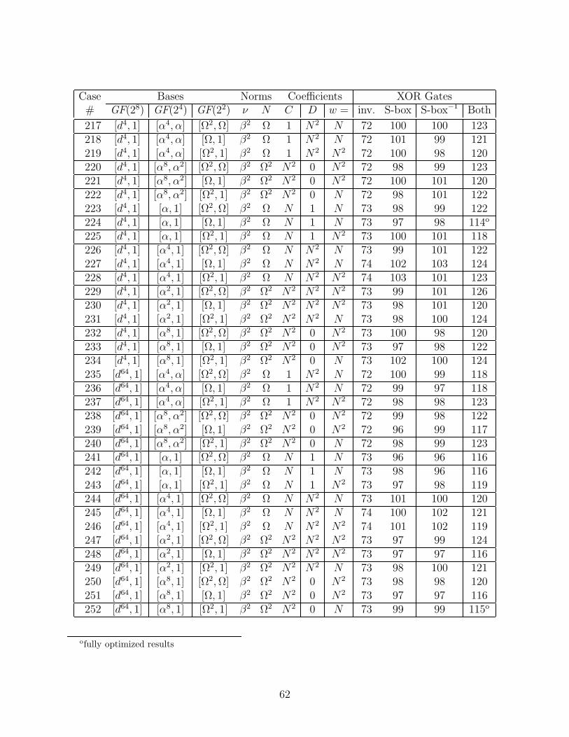
Case Bases Norms Coefficients XOR Gates# GF(28) GF(24) GF(22) ν N C D w = inv. S-box S-box−1 Both
217 [d4, 1] [α4, α] [Ω2, Ω] β2 Ω 1 N2 N 72 100 100 123218 [d4, 1] [α4, α] [Ω, 1] β2 Ω 1 N2 N 72 101 99 121219 [d4, 1] [α4, α] [Ω2, 1] β2 Ω 1 N2 N2 72 100 98 120220 [d4, 1] [α8, α2] [Ω2, Ω] β2 Ω2 N2 0 N2 72 98 99 123221 [d4, 1] [α8, α2] [Ω, 1] β2 Ω2 N2 0 N2 72 100 101 120222 [d4, 1] [α8, α2] [Ω2, 1] β2 Ω2 N2 0 N 72 98 101 122223 [d4, 1] [α, 1] [Ω2, Ω] β2 Ω N 1 N 73 98 99 122224 [d4, 1] [α, 1] [Ω, 1] β2 Ω N 1 N 73 97 98 114o
225 [d4, 1] [α, 1] [Ω2, 1] β2 Ω N 1 N2 73 100 101 118226 [d4, 1] [α4, 1] [Ω2, Ω] β2 Ω N N2 N 73 99 101 122227 [d4, 1] [α4, 1] [Ω, 1] β2 Ω N N2 N 74 102 103 124228 [d4, 1] [α4, 1] [Ω2, 1] β2 Ω N N2 N2 74 103 101 123229 [d4, 1] [α2, 1] [Ω2, Ω] β2 Ω2 N2 N2 N2 73 99 101 126230 [d4, 1] [α2, 1] [Ω, 1] β2 Ω2 N2 N2 N2 73 98 101 120231 [d4, 1] [α2, 1] [Ω2, 1] β2 Ω2 N2 N2 N 73 98 100 124232 [d4, 1] [α8, 1] [Ω2, Ω] β2 Ω2 N2 0 N2 73 100 98 120233 [d4, 1] [α8, 1] [Ω, 1] β2 Ω2 N2 0 N2 73 97 98 122234 [d4, 1] [α8, 1] [Ω2, 1] β2 Ω2 N2 0 N 73 102 100 124235 [d64, 1] [α4, α] [Ω2, Ω] β2 Ω 1 N2 N 72 100 99 118236 [d64, 1] [α4, α] [Ω, 1] β2 Ω 1 N2 N 72 99 97 118237 [d64, 1] [α4, α] [Ω2, 1] β2 Ω 1 N2 N2 72 98 98 123238 [d64, 1] [α8, α2] [Ω2, Ω] β2 Ω2 N2 0 N2 72 99 98 122239 [d64, 1] [α8, α2] [Ω, 1] β2 Ω2 N2 0 N2 72 96 99 117240 [d64, 1] [α8, α2] [Ω2, 1] β2 Ω2 N2 0 N 72 98 99 123241 [d64, 1] [α, 1] [Ω2, Ω] β2 Ω N 1 N 73 96 96 116242 [d64, 1] [α, 1] [Ω, 1] β2 Ω N 1 N 73 98 96 116243 [d64, 1] [α, 1] [Ω2, 1] β2 Ω N 1 N2 73 97 98 119244 [d64, 1] [α4, 1] [Ω2, Ω] β2 Ω N N2 N 73 101 100 120245 [d64, 1] [α4, 1] [Ω, 1] β2 Ω N N2 N 74 100 102 121246 [d64, 1] [α4, 1] [Ω2, 1] β2 Ω N N2 N2 74 101 102 119247 [d64, 1] [α2, 1] [Ω2, Ω] β2 Ω2 N2 N2 N2 73 97 99 124248 [d64, 1] [α2, 1] [Ω, 1] β2 Ω2 N2 N2 N2 73 97 97 116249 [d64, 1] [α2, 1] [Ω2, 1] β2 Ω2 N2 N2 N 73 98 100 121250 [d64, 1] [α8, 1] [Ω2, Ω] β2 Ω2 N2 0 N2 73 98 98 120251 [d64, 1] [α8, 1] [Ω, 1] β2 Ω2 N2 0 N2 73 97 97 116252 [d64, 1] [α8, 1] [Ω2, 1] β2 Ω2 N2 0 N 73 99 99 115o
ofully optimized results
62
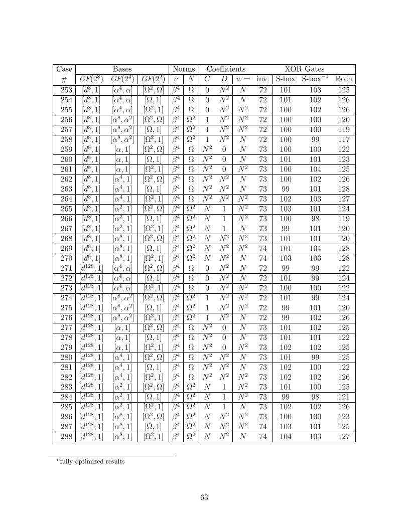
Case Bases Norms Coefficients XOR Gates# GF(28) GF(24) GF(22) ν N C D w = inv. S-box S-box−1 Both
253 [d8, 1] [α4, α] [Ω2, Ω] β4 Ω 0 N2 N 72 101 103 125254 [d8, 1] [α4, α] [Ω, 1] β4 Ω 0 N2 N 72 101 102 126255 [d8, 1] [α4, α] [Ω2, 1] β4 Ω 0 N2 N2 72 100 102 126256 [d8, 1] [α8, α2] [Ω2, Ω] β4 Ω2 1 N2 N2 72 100 100 120257 [d8, 1] [α8, α2] [Ω, 1] β4 Ω2 1 N2 N2 72 100 100 119258 [d8, 1] [α8, α2] [Ω2, 1] β4 Ω2 1 N2 N 72 100 99 117259 [d8, 1] [α, 1] [Ω2, Ω] β4 Ω N2 0 N 73 100 100 122260 [d8, 1] [α, 1] [Ω, 1] β4 Ω N2 0 N 73 101 101 123261 [d8, 1] [α, 1] [Ω2, 1] β4 Ω N2 0 N2 73 100 104 125262 [d8, 1] [α4, 1] [Ω2, Ω] β4 Ω N2 N2 N 73 100 102 126263 [d8, 1] [α4, 1] [Ω, 1] β4 Ω N2 N2 N 73 99 101 128264 [d8, 1] [α4, 1] [Ω2, 1] β4 Ω N2 N2 N2 73 102 103 127265 [d8, 1] [α2, 1] [Ω2, Ω] β4 Ω2 N 1 N2 73 103 101 124266 [d8, 1] [α2, 1] [Ω, 1] β4 Ω2 N 1 N2 73 100 98 119267 [d8, 1] [α2, 1] [Ω2, 1] β4 Ω2 N 1 N 73 99 101 120268 [d8, 1] [α8, 1] [Ω2, Ω] β4 Ω2 N N2 N2 73 101 101 120269 [d8, 1] [α8, 1] [Ω, 1] β4 Ω2 N N2 N2 74 101 104 128270 [d8, 1] [α8, 1] [Ω2, 1] β4 Ω2 N N2 N 74 103 103 128271 [d128, 1] [α4, α] [Ω2, Ω] β4 Ω 0 N2 N 72 99 99 122272 [d128, 1] [α4, α] [Ω, 1] β4 Ω 0 N2 N 72 101 99 124273 [d128, 1] [α4, α] [Ω2, 1] β4 Ω 0 N2 N2 72 100 100 122274 [d128, 1] [α8, α2] [Ω2, Ω] β4 Ω2 1 N2 N2 72 101 99 124275 [d128, 1] [α8, α2] [Ω, 1] β4 Ω2 1 N2 N2 72 99 101 120276 [d128, 1] [α8, α2] [Ω2, 1] β4 Ω2 1 N2 N 72 99 102 126277 [d128, 1] [α, 1] [Ω2, Ω] β4 Ω N2 0 N 73 101 102 125278 [d128, 1] [α, 1] [Ω, 1] β4 Ω N2 0 N 73 101 101 122279 [d128, 1] [α, 1] [Ω2, 1] β4 Ω N2 0 N2 73 102 102 125280 [d128, 1] [α4, 1] [Ω2, Ω] β4 Ω N2 N2 N 73 101 99 125281 [d128, 1] [α4, 1] [Ω, 1] β4 Ω N2 N2 N 73 102 100 122282 [d128, 1] [α4, 1] [Ω2, 1] β4 Ω N2 N2 N2 73 102 102 126283 [d128, 1] [α2, 1] [Ω2, Ω] β4 Ω2 N 1 N2 73 101 100 125284 [d128, 1] [α2, 1] [Ω, 1] β4 Ω2 N 1 N2 73 99 98 121285 [d128, 1] [α2, 1] [Ω2, 1] β4 Ω2 N 1 N 73 102 102 126286 [d128, 1] [α8, 1] [Ω2, Ω] β4 Ω2 N N2 N2 73 100 100 123287 [d128, 1] [α8, 1] [Ω, 1] β4 Ω2 N N2 N2 74 103 101 125288 [d128, 1] [α8, 1] [Ω2, 1] β4 Ω2 N N2 N 74 104 103 127
ofully optimized results
63
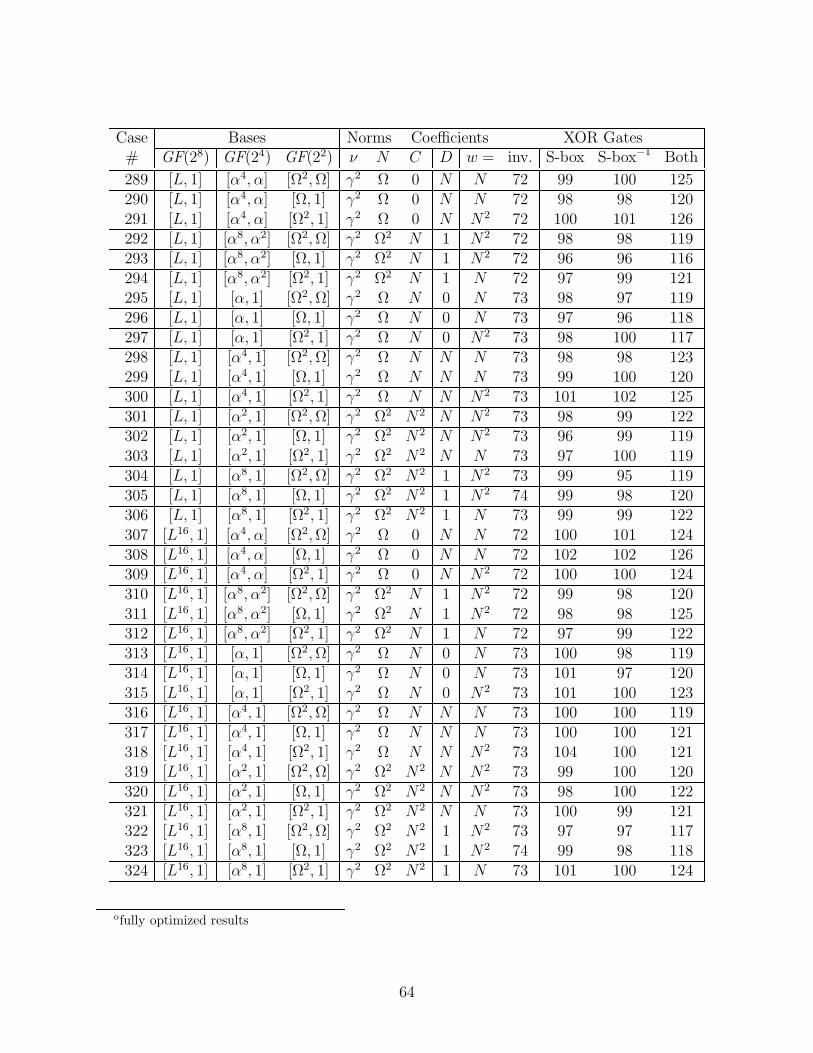
Case Bases Norms Coefficients XOR Gates# GF(28) GF(24) GF(22) ν N C D w = inv. S-box S-box−1 Both
289 [L, 1] [α4, α] [Ω2, Ω] γ2 Ω 0 N N 72 99 100 125290 [L, 1] [α4, α] [Ω, 1] γ2 Ω 0 N N 72 98 98 120291 [L, 1] [α4, α] [Ω2, 1] γ2 Ω 0 N N2 72 100 101 126292 [L, 1] [α8, α2] [Ω2, Ω] γ2 Ω2 N 1 N2 72 98 98 119293 [L, 1] [α8, α2] [Ω, 1] γ2 Ω2 N 1 N2 72 96 96 116294 [L, 1] [α8, α2] [Ω2, 1] γ2 Ω2 N 1 N 72 97 99 121295 [L, 1] [α, 1] [Ω2, Ω] γ2 Ω N 0 N 73 98 97 119296 [L, 1] [α, 1] [Ω, 1] γ2 Ω N 0 N 73 97 96 118297 [L, 1] [α, 1] [Ω2, 1] γ2 Ω N 0 N2 73 98 100 117298 [L, 1] [α4, 1] [Ω2, Ω] γ2 Ω N N N 73 98 98 123299 [L, 1] [α4, 1] [Ω, 1] γ2 Ω N N N 73 99 100 120300 [L, 1] [α4, 1] [Ω2, 1] γ2 Ω N N N2 73 101 102 125301 [L, 1] [α2, 1] [Ω2, Ω] γ2 Ω2 N2 N N2 73 98 99 122302 [L, 1] [α2, 1] [Ω, 1] γ2 Ω2 N2 N N2 73 96 99 119303 [L, 1] [α2, 1] [Ω2, 1] γ2 Ω2 N2 N N 73 97 100 119304 [L, 1] [α8, 1] [Ω2, Ω] γ2 Ω2 N2 1 N2 73 99 95 119305 [L, 1] [α8, 1] [Ω, 1] γ2 Ω2 N2 1 N2 74 99 98 120306 [L, 1] [α8, 1] [Ω2, 1] γ2 Ω2 N2 1 N 73 99 99 122307 [L16, 1] [α4, α] [Ω2, Ω] γ2 Ω 0 N N 72 100 101 124308 [L16, 1] [α4, α] [Ω, 1] γ2 Ω 0 N N 72 102 102 126309 [L16, 1] [α4, α] [Ω2, 1] γ2 Ω 0 N N2 72 100 100 124310 [L16, 1] [α8, α2] [Ω2, Ω] γ2 Ω2 N 1 N2 72 99 98 120311 [L16, 1] [α8, α2] [Ω, 1] γ2 Ω2 N 1 N2 72 98 98 125312 [L16, 1] [α8, α2] [Ω2, 1] γ2 Ω2 N 1 N 72 97 99 122313 [L16, 1] [α, 1] [Ω2, Ω] γ2 Ω N 0 N 73 100 98 119314 [L16, 1] [α, 1] [Ω, 1] γ2 Ω N 0 N 73 101 97 120315 [L16, 1] [α, 1] [Ω2, 1] γ2 Ω N 0 N2 73 101 100 123316 [L16, 1] [α4, 1] [Ω2, Ω] γ2 Ω N N N 73 100 100 119317 [L16, 1] [α4, 1] [Ω, 1] γ2 Ω N N N 73 100 100 121318 [L16, 1] [α4, 1] [Ω2, 1] γ2 Ω N N N2 73 104 100 121319 [L16, 1] [α2, 1] [Ω2, Ω] γ2 Ω2 N2 N N2 73 99 100 120320 [L16, 1] [α2, 1] [Ω, 1] γ2 Ω2 N2 N N2 73 98 100 122321 [L16, 1] [α2, 1] [Ω2, 1] γ2 Ω2 N2 N N 73 100 99 121322 [L16, 1] [α8, 1] [Ω2, Ω] γ2 Ω2 N2 1 N2 73 97 97 117323 [L16, 1] [α8, 1] [Ω, 1] γ2 Ω2 N2 1 N2 74 99 98 118324 [L16, 1] [α8, 1] [Ω2, 1] γ2 Ω2 N2 1 N 73 101 100 124
ofully optimized results
64

Case Bases Norms Coefficients XOR Gates# GF(28) GF(24) GF(22) ν N C D w = inv. S-box S-box−1 Both
325 [L2, 1] [α4, α] [Ω2, Ω] γ4 Ω 1 N N 72 99 99 124326 [L2, 1] [α4, α] [Ω, 1] γ4 Ω 1 N N 72 98 99 122327 [L2, 1] [α4, α] [Ω2, 1] γ4 Ω 1 N N2 72 99 99 127328 [L2, 1] [α8, α2] [Ω2, Ω] γ4 Ω2 0 N N2 72 97 99 116329 [L2, 1] [α8, α2] [Ω, 1] γ4 Ω2 0 N N2 72 98 100 124330 [L2, 1] [α8, α2] [Ω2, 1] γ4 Ω2 0 N N 72 98 99 118331 [L2, 1] [α, 1] [Ω2, Ω] γ4 Ω N2 1 N 73 101 102 123332 [L2, 1] [α, 1] [Ω, 1] γ4 Ω N2 1 N 73 101 101 124333 [L2, 1] [α, 1] [Ω2, 1] γ4 Ω N2 1 N2 74 101 104 124334 [L2, 1] [α4, 1] [Ω2, Ω] γ4 Ω N2 N N 73 99 99 120335 [L2, 1] [α4, 1] [Ω, 1] γ4 Ω N2 N N 73 98 97 121336 [L2, 1] [α4, 1] [Ω2, 1] γ4 Ω N2 N N2 73 99 100 121337 [L2, 1] [α2, 1] [Ω2, Ω] γ4 Ω2 N 0 N2 73 100 102 126338 [L2, 1] [α2, 1] [Ω, 1] γ4 Ω2 N 0 N2 73 99 102 125339 [L2, 1] [α2, 1] [Ω2, 1] γ4 Ω2 N 0 N 73 100 103 124340 [L2, 1] [α8, 1] [Ω2, Ω] γ4 Ω2 N N N2 73 99 98 118341 [L2, 1] [α8, 1] [Ω, 1] γ4 Ω2 N N N2 73 101 102 123342 [L2, 1] [α8, 1] [Ω2, 1] γ4 Ω2 N N N 73 101 102 124343 [L32, 1] [α4, α] [Ω2, Ω] γ4 Ω 1 N N 72 100 103 126344 [L32, 1] [α4, α] [Ω, 1] γ4 Ω 1 N N 72 101 100 125345 [L32, 1] [α4, α] [Ω2, 1] γ4 Ω 1 N N2 72 102 103 127346 [L32, 1] [α8, α2] [Ω2, Ω] γ4 Ω2 0 N N2 72 101 99 123347 [L32, 1] [α8, α2] [Ω, 1] γ4 Ω2 0 N N2 72 96 96 117348 [L32, 1] [α8, α2] [Ω2, 1] γ4 Ω2 0 N N 72 99 98 120349 [L32, 1] [α, 1] [Ω2, Ω] γ4 Ω N2 1 N 73 102 103 130350 [L32, 1] [α, 1] [Ω, 1] γ4 Ω N2 1 N 73 102 101 125351 [L32, 1] [α, 1] [Ω2, 1] γ4 Ω N2 1 N2 74 103 104 129352 [L32, 1] [α4, 1] [Ω2, Ω] γ4 Ω N2 N N 73 102 101 126353 [L32, 1] [α4, 1] [Ω, 1] γ4 Ω N2 N N 73 101 102 126354 [L32, 1] [α4, 1] [Ω2, 1] γ4 Ω N2 N N2 73 103 102 128355 [L32, 1] [α2, 1] [Ω2, Ω] γ4 Ω2 N 0 N2 73 102 101 124356 [L32, 1] [α2, 1] [Ω, 1] γ4 Ω2 N 0 N2 73 99 99 118357 [L32, 1] [α2, 1] [Ω2, 1] γ4 Ω2 N 0 N 73 99 102 125358 [L32, 1] [α8, 1] [Ω2, Ω] γ4 Ω2 N N N2 73 102 100 124359 [L32, 1] [α8, 1] [Ω, 1] γ4 Ω2 N N N2 73 100 100 124360 [L32, 1] [α8, 1] [Ω2, 1] γ4 Ω2 N N N 73 100 102 122
ofully optimized results
65
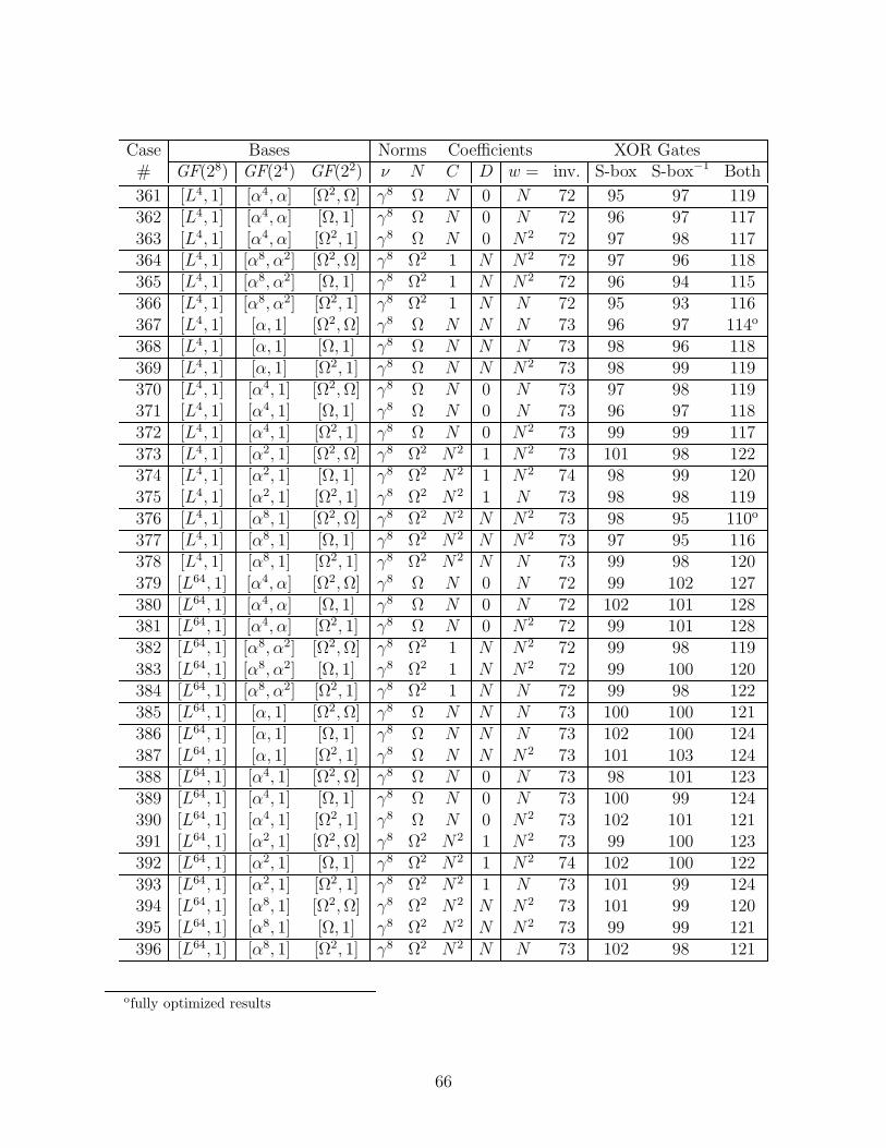
Case Bases Norms Coefficients XOR Gates# GF(28) GF(24) GF(22) ν N C D w = inv. S-box S-box−1 Both
361 [L4, 1] [α4, α] [Ω2, Ω] γ8 Ω N 0 N 72 95 97 119362 [L4, 1] [α4, α] [Ω, 1] γ8 Ω N 0 N 72 96 97 117363 [L4, 1] [α4, α] [Ω2, 1] γ8 Ω N 0 N2 72 97 98 117364 [L4, 1] [α8, α2] [Ω2, Ω] γ8 Ω2 1 N N2 72 97 96 118365 [L4, 1] [α8, α2] [Ω, 1] γ8 Ω2 1 N N2 72 96 94 115366 [L4, 1] [α8, α2] [Ω2, 1] γ8 Ω2 1 N N 72 95 93 116367 [L4, 1] [α, 1] [Ω2, Ω] γ8 Ω N N N 73 96 97 114o
368 [L4, 1] [α, 1] [Ω, 1] γ8 Ω N N N 73 98 96 118369 [L4, 1] [α, 1] [Ω2, 1] γ8 Ω N N N2 73 98 99 119370 [L4, 1] [α4, 1] [Ω2, Ω] γ8 Ω N 0 N 73 97 98 119371 [L4, 1] [α4, 1] [Ω, 1] γ8 Ω N 0 N 73 96 97 118372 [L4, 1] [α4, 1] [Ω2, 1] γ8 Ω N 0 N2 73 99 99 117373 [L4, 1] [α2, 1] [Ω2, Ω] γ8 Ω2 N2 1 N2 73 101 98 122374 [L4, 1] [α2, 1] [Ω, 1] γ8 Ω2 N2 1 N2 74 98 99 120375 [L4, 1] [α2, 1] [Ω2, 1] γ8 Ω2 N2 1 N 73 98 98 119376 [L4, 1] [α8, 1] [Ω2, Ω] γ8 Ω2 N2 N N2 73 98 95 110o
377 [L4, 1] [α8, 1] [Ω, 1] γ8 Ω2 N2 N N2 73 97 95 116378 [L4, 1] [α8, 1] [Ω2, 1] γ8 Ω2 N2 N N 73 99 98 120379 [L64, 1] [α4, α] [Ω2, Ω] γ8 Ω N 0 N 72 99 102 127380 [L64, 1] [α4, α] [Ω, 1] γ8 Ω N 0 N 72 102 101 128381 [L64, 1] [α4, α] [Ω2, 1] γ8 Ω N 0 N2 72 99 101 128382 [L64, 1] [α8, α2] [Ω2, Ω] γ8 Ω2 1 N N2 72 99 98 119383 [L64, 1] [α8, α2] [Ω, 1] γ8 Ω2 1 N N2 72 99 100 120384 [L64, 1] [α8, α2] [Ω2, 1] γ8 Ω2 1 N N 72 99 98 122385 [L64, 1] [α, 1] [Ω2, Ω] γ8 Ω N N N 73 100 100 121386 [L64, 1] [α, 1] [Ω, 1] γ8 Ω N N N 73 102 100 124387 [L64, 1] [α, 1] [Ω2, 1] γ8 Ω N N N2 73 101 103 124388 [L64, 1] [α4, 1] [Ω2, Ω] γ8 Ω N 0 N 73 98 101 123389 [L64, 1] [α4, 1] [Ω, 1] γ8 Ω N 0 N 73 100 99 124390 [L64, 1] [α4, 1] [Ω2, 1] γ8 Ω N 0 N2 73 102 101 121391 [L64, 1] [α2, 1] [Ω2, Ω] γ8 Ω2 N2 1 N2 73 99 100 123392 [L64, 1] [α2, 1] [Ω, 1] γ8 Ω2 N2 1 N2 74 102 100 122393 [L64, 1] [α2, 1] [Ω2, 1] γ8 Ω2 N2 1 N 73 101 99 124394 [L64, 1] [α8, 1] [Ω2, Ω] γ8 Ω2 N2 N N2 73 101 99 120395 [L64, 1] [α8, 1] [Ω, 1] γ8 Ω2 N2 N N2 73 99 99 121396 [L64, 1] [α8, 1] [Ω2, 1] γ8 Ω2 N2 N N 73 102 98 121
ofully optimized results
66

Case Bases Norms Coefficients XOR Gates# GF(28) GF(24) GF(22) ν N C D w = inv. S-box S-box−1 Both
397 [L8, 1] [α4, α] [Ω2, Ω] γ Ω N 1 N 72 102 103 125398 [L8, 1] [α4, α] [Ω, 1] γ Ω N 1 N 72 101 101 123399 [L8, 1] [α4, α] [Ω2, 1] γ Ω N 1 N2 72 103 102 123400 [L8, 1] [α8, α2] [Ω2, Ω] γ Ω2 N 0 N2 72 99 101 120401 [L8, 1] [α8, α2] [Ω, 1] γ Ω2 N 0 N2 72 99 100 119402 [L8, 1] [α8, α2] [Ω2, 1] γ Ω2 N 0 N 72 99 98 121403 [L8, 1] [α, 1] [Ω2, Ω] γ Ω N2 N N 73 101 103 123404 [L8, 1] [α, 1] [Ω, 1] γ Ω N2 N N 73 101 103 120405 [L8, 1] [α, 1] [Ω2, 1] γ Ω N2 N N2 73 102 106 123406 [L8, 1] [α4, 1] [Ω2, Ω] γ Ω N2 1 N 73 102 104 129407 [L8, 1] [α4, 1] [Ω, 1] γ Ω N2 1 N 73 101 103 125408 [L8, 1] [α4, 1] [Ω2, 1] γ Ω N2 1 N2 74 103 104 128409 [L8, 1] [α2, 1] [Ω2, Ω] γ Ω2 N N N2 73 102 102 125410 [L8, 1] [α2, 1] [Ω, 1] γ Ω2 N N N2 73 99 103 121411 [L8, 1] [α2, 1] [Ω2, 1] γ Ω2 N N N 73 101 102 125412 [L8, 1] [α8, 1] [Ω2, Ω] γ Ω2 N 0 N2 73 101 100 121413 [L8, 1] [α8, 1] [Ω, 1] γ Ω2 N 0 N2 73 101 101 119414 [L8, 1] [α8, 1] [Ω2, 1] γ Ω2 N 0 N 73 100 101 123415 [L128, 1] [α4, α] [Ω2, Ω] γ Ω N 1 N 72 100 101 127416 [L128, 1] [α4, α] [Ω, 1] γ Ω N 1 N 72 101 100 120417 [L128, 1] [α4, α] [Ω2, 1] γ Ω N 1 N2 72 102 103 128418 [L128, 1] [α8, α2] [Ω2, Ω] γ Ω2 N 0 N2 72 98 99 118419 [L128, 1] [α8, α2] [Ω, 1] γ Ω2 N 0 N2 72 97 101 122420 [L128, 1] [α8, α2] [Ω2, 1] γ Ω2 N 0 N 72 100 100 123421 [L128, 1] [α, 1] [Ω2, Ω] γ Ω N2 N N 73 101 104 122422 [L128, 1] [α, 1] [Ω, 1] γ Ω N2 N N 73 101 100 122423 [L128, 1] [α, 1] [Ω2, 1] γ Ω N2 N N2 73 102 103 127424 [L128, 1] [α4, 1] [Ω2, Ω] γ Ω N2 1 N 73 103 103 126425 [L128, 1] [α4, 1] [Ω, 1] γ Ω N2 1 N 73 100 101 125426 [L128, 1] [α4, 1] [Ω2, 1] γ Ω N2 1 N2 74 106 105 131427 [L128, 1] [α2, 1] [Ω2, Ω] γ Ω2 N N N2 73 101 102 124428 [L128, 1] [α2, 1] [Ω, 1] γ Ω2 N N N2 73 99 101 122429 [L128, 1] [α2, 1] [Ω2, 1] γ Ω2 N N N 73 100 104 128430 [L128, 1] [α8, 1] [Ω2, Ω] γ Ω2 N 0 N2 73 98 100 118431 [L128, 1] [α8, 1] [Ω, 1] γ Ω2 N 0 N2 73 97 99 120432 [L128, 1] [α8, 1] [Ω2, 1] γ Ω2 N 0 N 73 101 101 121
ofully optimized results
67

INITIAL DISTRIBUTION LIST 1. Defense Technical Information Center 2
8725 John J. Kingman Rd., STE 0944 Ft. Belvoir, VA 22060-6218
2. Dudley Knox Library, Code 013 2
Naval Postgraduate School Monterey, CA 93943-5100
3. Alan Hunsberger 2
National Security Agency 9800 Savage Road, Ste. 6538 Fort Meade, MD 20755-6538
4. Douglas Fouts, Code EC/Fs 1
Naval Postgraduate School Monterey, CA 93943-5207
5. David Canright, Code MA/Ca 10
Naval Postgraduate School Monterey, CA 93943-5216