NAVAL POSTGRADUATE

SCHOOL

MONTEREY, CA

OC3570 –PROJECT

A STUDY OF THE UNDERSEA CURRENTS WITHIN THE SAN NICHOLAS BASIN, SOUTHWEST OF SAN CLEMENTE ISLAND,

CALIFORNIA

by

LT David Colbert

September 2009

I. INTRODUCTION

The purpose of this study is to determine the undersea currents within the San

Nicholas Basin (SNB) using an Acoustic Doppler Current Profiler (ADCP). The

Teledyne RD Instruments (RDI) Ocean Surveyor Acoustic Doppler Current Profiler

(OSADCP) is the system mounted on the R/V New Horizon to acquire necessary

subsurface current data. The Naval Post-graduate School (NPS), research team embarked

on the vessel collection the data for the project. The ship departed from San Diego, CA

on July 24th and returned to San Diego on July 28th, 2009.

The SNB offers an excellent site for this project. It is a deep water basin that has

been studied before. Located relatively close to San Diego, CA the basin is nestled

between San Clemente Island to the east and San Nicholas Island to the west. During the

four days aboard the R/V New Horizon the ship passed directly over the basin two times.

These transits in conjunction with earlier findings (Gay, 2009) offer more than enough

data to accurately determine the location, velocity, and direction of the undersea current.

The vessel deployed for this project as stated earlier is the R/V New Horizon. This

platform turned out to be a perfect match for the expedition. The 170 foot ship was built

in 1978 and is owned by the University of California, San Diego. Its primary purpose is

oceanographic research and is operated by the Scripps Institute of Oceanography. The

navigation capabilities aboard the R/V New Horizon are the Trimble NT 300 differential

GPS, Ashtech ADU attitude sensing system, Trimble Tansmon P-code GPS, and the

Ametek Doppler Speed Log (R/V New Horizon, 2009).

2

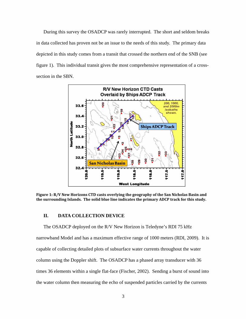
During this survey the OSADCP was rarely interrupted. The short and seldom breaks

in data collected has proven not be an issue to the needs of this study. The primary data

depicted in this study comes from a transit that crossed the northern end of the SNB (see

figure 1). This individual transit gives the most comprehensive representation of a cross-

section in the SBN.

Figure 1: R/V New Horizons CTD casts overlying the geography of the San Nicholas Basin and the surrounding Islands.  The solid blue line indicates the primary ADCP track for this study. 

II. DATA COLLECTION DEVICE

The OSADCP deployed on the R/V New Horizon is Teledyne’s RDI 75 kHz

narrowband Model and has a maximum effective range of 1000 meters (RDI, 2009). It is

capable of collecting detailed plots of subsurface water currents throughout the water

column using the Doppler shift. The OSADCP has a phased array transducer with 36

times 36 elements within a single flat-face (Fischer, 2002). Sending a burst of sound into

the water column then measuring the echo of suspended particles carried by the currents

3

as they pass multiple receptor cells within the OSADCP. Echoes that are retrieved later

are given as deeper recording. Through this and in conjunction with the ships navigation,

it can determine the velocity and direction of flow throughout the column. The OSADCP

has the option of operating in both narrow-band and broad-band. For this study we used

the narrow-band.

III. DATA PROCESSING

The data collected by the OSADCP aboard the R/V New Horizon was averaged and

saved every 5 minutes then updated every hour and stored in a Common Ocean Data

Access System (CODAS) database. The CODAS allows easier processing (as well as

underway formatting) of the ADCP data. The software used to process the CODAS is

named after the University of Hawaii Data Assimilation Software (UHDAS) and it comes

from the University of Hawaii, Department of Oceanography (Hammon, 2009). The

UHDAS enables the operator to turn the OSADCP data into a readable format that allows

the user to view the subsurface current profile graphically. This procedure is a multistep

process that corrects the data and enables the operator to make corrections so that the

result is valuable to the scientific community. All post processing for the OSADCP was

completed by the research teams Chief Scientist, Dr. Curtis A. Collins a professor from

NPS.

The OSADCP sea surface temperature (SST) is first checked to determine if the

sound speed is accurate at the transducer. This is accomplished using a plot of OSADCP

temperature verses the shipboard systems such as the boom probe (hung over the aft-port

of the vessel), the ships intake that utilizes a Seabird Electronics (SBE) 45 MicroTSG

4

Thermosalinograph, and also the vessel’s overboard Conductivity Temperature Depth

profiler (CTD) (see figure 2).

24/07 25/07 26/07 27/07 28/07 29/0716

17

18

19

20

21

22

23

24

Co

SST Comparison R/V New Horizon, 24-28 July 2009

adcp

sstboom

ctd

Figure 2: A C° verses time plot comparing the SST detection devises aboard the RV New Horizon.  The red line depicts the ADCP, the blue line depicts the ships intake, the black line depicts the overboard boom, and the green plus indicate individual CTD casts.  

In this comparison we find that the OSADCP seems to follow a similar pattern as the

boom, intake thermometers, and the CTD’s SST, but shows a visible lag of roughly a day.

This is a concern for it could indicate a problem with the collection device. The next step

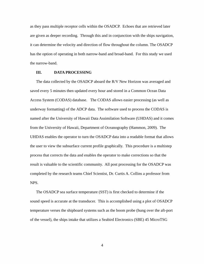
is to check the OSADCP’s longitude compared to the ships longitude (see figure 3). In

this comparison the adcp designates the OSADCP with a solid red line and the ships met

data is designated with a solid blue line. This shows that the ADCP’s position is equal to

the ships. There are very few places along the longitude verses time plot that the red line

is even visible. This is an indication that the OSADCP’s presumed spatial location is

highly accurate while the temperature sensor is not. This does not specifically point to a

5

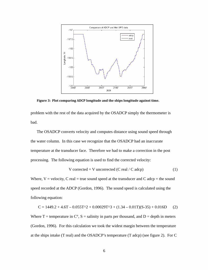
Figure 3:  Plot comparing ADCP longitude and the ships longitude against time.  

problem with the rest of the data acquired by the OSADCP simply the thermometer is

bad.

The OSADCP converts velocity and computes distance using sound speed through

the water column. In this case we recognize that the OSADCP had an inaccurate

temperature at the transducer face. Therefore we had to make a correction in the post

processing. The following equation is used to find the corrected velocity:

V corrected = V uncorrected (C real / C adcp) (1)

Where, V = velocity, C real = true sound speed at the transducer and C adcp = the sound

speed recorded at the ADCP (Gordon, 1996). The sound speed is calculated using the

following equation:

C = 1449.2 + 4.6T – 0.055T^2 + 0.00029T^3 + (1.34 – 0.01T)(S-35) + 0.016D (2)

Where T = temperature in C°, S = salinity in parts per thousand, and D = depth in meters

(Gordon, 1996). For this calculation we took the widest margin between the temperature

at the ships intake (T real) and the OSADCP’s temperature (T adcp) (see figure 2). For C

6

real we find a sound speed of 1520.63 m/s and the sound speed for C adcp as 1526.72

m/s. When computed we have a (C real / C adcp) equal to 0.9986. This outcome is very

close to 1 so we determine that the V uncorrected is very close to the V corrected.

Therefore we do not need to adjust the data for velocity.

As state earlier primary OSADCP transit crosses the northern end of the SNB, with a

relative heading northeast to southwest. This track is rotated by 54.5 ° to ease the

processing and reading of the data collected. This heading also varies from CTD station

to CTD station (as we adjusted heading for better seas while on station). The average

velocity of the subsurface current between 50-100 meters was calculated and compared to

the geostrophic velocity of the same depth (see figure 4).

Figure 4:  Plot comparing ADCP velocity and geostrophic velocity with longitude.   In this comparison there is a similar trend in both velocities. The ADCP velocity does

seem to be more varied with higher peaks and lower troughs. Therefore we smooth the

data from the OSADCP by limiting the interval to 12 data points (see figure 5). This

brought the OSADCP velocity closer to the geostrophic velocity.

7

Figure 5:   This plot compares a ADCP velocity that has been smoothed to 12 data points and geostrophic velocity both verses longitude.  The blue dots are the geostrophic velocities data points overlaid on the ADCP velocities.   

As stated earlier part of the ships navigation is the Ashtech ADU attitude sensing

system (Ashtech Gyro) this has to be compared to the true heading from GPS. Heading

errors can have a profound impact on the currents speed and direction (see figure 6). The

OSADCP data has to be corrected for the time variable gyro heading errors due to the

Figure 6:  Difference between Ashtech Gyro heading and degrees true verses decimal date. 

8

Schuler Oscillations compared to the GPS heading. This plot shows a relatively

significant error in the Ships Gyro. There is a trend to the positive side although there

does seem to be quite a bit of variation across the board. This is applied to the data as a

correction to heading.

The operator then reviews the data and can “zap” (remove) bad or extraneous data

from the final produce. This bad data will be outliers that could not be a reality in the

subsurface waters (see figure 7).

Figure 7:  Absolute reference layer velocity compared to the U axis verses decimal date and Absolute reference layer velocity compared to the V axis verses decimal date.   The reference layer velocity sited is the 50-100 meter depth velocity from the cruise. It is

measured in meters per second with U as the along track velocity and V as the cross-

section velocity. If left unchecked these uncorrected data points would lead to a false

depiction of the subsurface currents, their velocities and their directions. The data shown

above has had its extraneous outliers cleaned.

For the OSADCP to have the correct heading there are many factors that come into

play. The alignment of the ships axis and the calibration of the OSADCP is crucial for

the accuracy of the subsurface currents. The misalignment of the ADCP can usually be

traced to at least one of two factors. The first would be simply a skewed mounting of the

transducer head against the ships axis. This is apparently the more common of the

9

misalignment (Fischer, 2009). The second is the ships compass synchronization having

an unknown offset in opposition to the ADCP deck unit. The inaccurate calibration of the

OSADCP and the ships axis will cause a misreading of the acceleration and/or

deceleration of the subsurface currents. This will be exacerbated as the ship speeds up

and when the ship reaches an on-station location. For this study we used the “water

tracking” determination method. This method uses the fact that in a small region the

currents will remain relatively constant. Therefore this level of inaccuracy will be

evident as the ship approached the station at speed or rapidly changes heading as opposed

to on-station readings. We have multiple CTD drops where the ship decelerated and

changed heading to stay on-station during the four days of OSADCP data gathering.

Each of these CTD casts can be used as benchmarks for the water tracking method.

IV. RESULTS

Once the data has been corrected and processed through UHDAS the water column is

plotted. The processed data is then trimmed to the section that we are most interested in

for this study, the transit across the northern end of the SNB (see figure 1). This track

along with the other track that crosses the SBN from the west side of San Clemente

Island (SCI), indicates a strong current that flows to the north-northwest (see figure 8).

This current depicted in figure 8 is exactly the current Gay and Chereskin describe in

there “Undercurrent off Southern California”. They found that the current was strongest

along the eastern edge of the SBN. The date collected on the R/V New Horizon show the

same tendency with a top speed of roughly 40 cm/sec to the west of SCI. The Strength

and location of the current is shown in the along-section view of the velocity

10

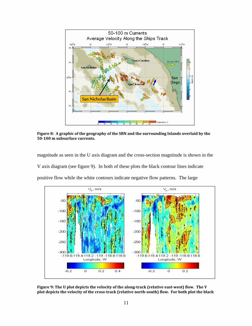
Figure 8:  A graphic of the geography of the SBN and the surrounding Islands overlaid by the 50­100 m subsurface currents.   

magnitude as seen in the U axis diagram and the cross-section magnitude is shown in the

V axis diagram (see figure 9). In both of these plots the black contour lines indicate

positive flow while the white contours indicate negative flow patterns. The large

Figure 9: The U plot depicts the velocity of the along­track (relative east­west) flow.  The V plot depicts the velocity of the cross­track (relative north­south) flow.  For both plot the black 

11

contours indicate positive flow direction (into the page) and the white contours indicate negative flow direction (out of the page).   whiteout area to the lower left is the Tanner Bank (TB) that acts as the western boundary

of the SNB. The whiteout area on the far right of the graphics is SCI rising from the sea

floor.

The U or along-section flow plot shows evidence of a strong surge traversing from

the west to the east over the TB. This helps fuel the larger more powerful current that is

seen in the V or cross-section flow plot. In the cross-section flow graphic we do find the

current we expected to find dominating the 50-100 meter depth of the SNB and running

in a relative northerly direction.

When the entire four day vessel track is plotted and displayed with the average 50-

100 meter currents we have a diagram that proves the subsurface current exists. It is a

counter current flowing in a north-northwesterly direction through the SNB (see figure

10).

12

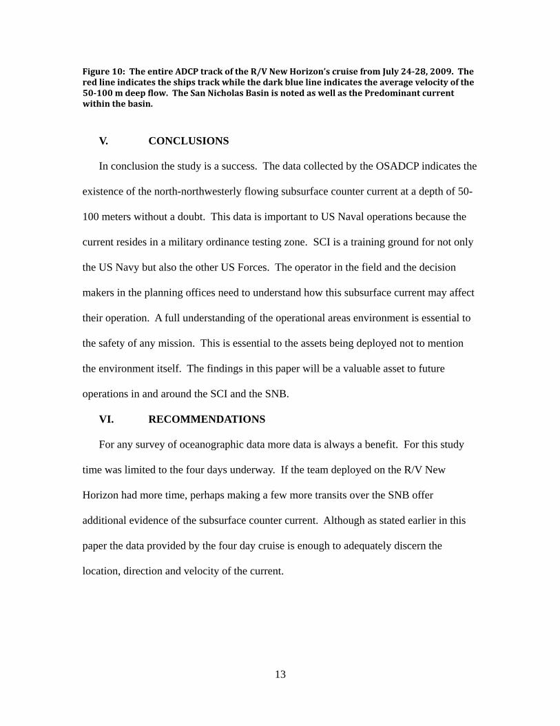
Figure 10:  The entire ADCP track of the R/V New Horizon’s cruise from July 24­28, 2009.  The red line indicates the ships track while the dark blue line indicates the average velocity of the 50­100 m deep flow.  The San Nicholas Basin is noted as well as the Predominant current within the basin. 

V. CONCLUSIONS

In conclusion the study is a success. The data collected by the OSADCP indicates the

existence of the north-northwesterly flowing subsurface counter current at a depth of 50-

100 meters without a doubt. This data is important to US Naval operations because the

current resides in a military ordinance testing zone. SCI is a training ground for not only

the US Navy but also the other US Forces. The operator in the field and the decision

makers in the planning offices need to understand how this subsurface current may affect

their operation. A full understanding of the operational areas environment is essential to

the safety of any mission. This is essential to the assets being deployed not to mention

the environment itself. The findings in this paper will be a valuable asset to future

operations in and around the SCI and the SNB.

VI. RECOMMENDATIONS

For any survey of oceanographic data more data is always a benefit. For this study

time was limited to the four days underway. If the team deployed on the R/V New

Horizon had more time, perhaps making a few more transits over the SNB offer

additional evidence of the subsurface counter current. Although as stated earlier in this

paper the data provided by the four day cruise is enough to adequately discern the

location, direction and velocity of the current.

13

14

VII. REFERENSES

Gay, P. S., T. K. Chereskin, (2009), Mean structure and seasonal variability of the

poleward undercurrent off southern California, J. Geophy. Research, 114, CO2007 R/V New Horizon Handbook, Scripps Institution of Oceanography, UC San Diego, 15

Sept. 2009 <http://shipsked.ucsd.edu/Ships/New_Horizon/Handbook/>. RD Instruments Ocean Surveyor ADCP, Teledyne Technologies Incorporated, 15 Sept.

2009 < http://www.rdinstruments.com/surveyor.aspx>. Fischer, J., P. Brandt, M. Dengler, M. Muller, (2002), Surveying the upper ocean with the

ocean surveyor: a new phased array Doppler current profiler. J. Atmos. Oceanis Technol., 20, 742-751.

Hammon, J., UHDAS+CODAS Documentation, University of Hawaii Dept. of

Oceanography, 15 Sept. 2009 < http://currents.soest.hawaii.edu/docs/doc/>. Gordon, R. L. (1996), Acoustic Doppler current profiler, Principles of Operation A

Practical Primer, RD Instruments.