NBER WORKING PAPER SERIES

EVALUATING THE EFFECT OF ANANTIDISCRIMINATION LAW USING

A REGRESSION-DISCONTINUITY DESIGN

Jinyong HahnPetra Todd

Wilbert Van der Klaauw

Working Paper 7131http://www.nber.org/papers/w7 131

NATIONAL BUREAU OF ECONOMIC RESEARCH1050 Massachusetts Avenue

Cambridge, MA 02138May 1999

A previous version of this paper has been circulated under the title "Estimation of Treatment Effects witha Quasi-Experimental Regression-Discontinuity Design: with Application to Evaluating the Effect ofFederal Antidiscrimination Laws on Minority Employment in Small U.S. Firms." We thank Joshua Angrist,James Heckman, Guido Imbens, Alan Kruegger, Tony Lancaster, Sendhil Mullainathan, and Ken Wolpinfor helpful comments. The paper has also benefited from comments received at the 1997 MidwesternEconometrics Group conference, the 1997 AEA meetings, the 1998 Econometric Society Summer Meetingsin Montreal, the University of Michigan, the University of Rochester, the University of Wisconsin, the jointHarvard/MIT econometrics conference, and the joint Brown-Yale-NYU-Penn-JHU labor conference. Vander Klaauw thanks the C.V. Starr Center of Applied Economics at NYU for research support. Petra Todd'sparticipation was supported by NSF grant #SBR-9730688. The views expressed herein are those of theauthors and do not necessarily reflect the views of the National Bureau of Economic Research.

© 1999 by Jinyong Hahn, Petra Todd, and Wilbert Van der Klaauw. All rights reserved. Short sections oftext, not to exceed two paragraphs, may be quoted without explicit permission provided that full credit,including © notice, is given to the source.

Evaluating the Effect of an AntidiscriminationLaw using a Regression-Discontinuity DesignJinyong Hahn, Petra Todd, and Wilbert Van der KlaauwNBER Working Paper No. 7131May 1999JELNo. C14, C51

ABSTRACT

The regression discontinuity (RD) data design is a quasi-experimental design with the

defining characteristic that the probability of receiving treatment changes discontinuously as a

function of one or more individual characteristics. This data design occasionally arises in economic

and other applications but is only infrequently exploited in evaluating the effects of a treatment. We

consider the problem of identification and estimation of treatment effects under a RD data design.

We offer an interpretation of the IV or so-called Wald estimator as a regression discontinuity

estimator. We propose nonparametric estimators of treatment effects and present their asymptotic

distribution theory. Then we apply the estimation method to evaluate the effect of EEOC-coverage

on minority employment in small U.S. firms.

Jinyong Hahn Petra ToddDepartment of Economics Department of Economics

University of Pennsylvania University of Pennsylvania3718 Locust Walk 3718 Locust WalkPhiladelphia, PA 19104 Philadelphia, PA 19104

hahn@econ.sas.upenn.edu and NBER

petraathena.sas.upenn.edu

Wilbert van der KlaauwDepartment of EconomicsUniversity of North CarolinaChapel Hill, NC 27599

1 Introduction

Quasi-experimental methods, like the regression-discontinuity method, are only infrequently consid-ered in the evaluation literature as a separate method of evaluation. The focus is usually either on

purely experimental or purely observational methods. Data generated by a regression-discontinuity

design shares features with both experimental and observational data. In an experiment, treat-

ment is assigned by a randomization device, which guarantees that persons in the treated group

and in the control group are comparable. A regression-discontinuity (RD) design is similar to anexperiment in that there is also a known rule that influences how persons are assigned to treat-

ment. However, assignment to treatment is not random and persons who receive treatment may

differ systematically from those who do not. In this sense, data from a RD design are similar toobservational data.

In one of the first applications of the RD method and the first paper to introduce the design,

Thistlethwaite and Campbell (1960) estimate the effect that receipt of a National Merit Award has

on students' success in obtaining additional college scholarships and on their career aspirations.

They observe that the awards are given on the basis of whether a test score exceeds a threshold, so

one can take advantage of knowing the cut-off point to learn about treatment effects for persons near

the cut-off. Berk and Rauma (1983) take a similar approach in analyzing the effect of extending

unemployment benefits to released prisoners on recidivism rates, where benefits are given only to

prisoners who worked a minimum number of hours while in prison. Van der Klaauw (1996) examines

the effect that college scholarships awarded at the time of admission have on students' decisions

to attend a particular college. He uses the fact that the value of an index based on a combination

of the student's grade-point average and SAT score partly determines in a discontinuous manner

whether a fellowship is awarded as well as the amount of fellowship. In another recent application,

Angrist and Lavy (1996) estimate the effect of classroom size on student test scores. One of thefactors determining class size in their data is a rule stipulating that another classroom be added

whenever the average classroom size crosses a threshold level. Finally, Black (1996) uses an RD

approach to estimate parents' willingness to pay for higher quality schools by comparing housingprices near geographic school attendance boundaries. In all these examples, the treatment variable

changes discontinuously as a function of one or more underlying variables, which is the defining

characteristic of regression discontinuity data designs.

Although there have already been many applications of RD methods, important questions stillremain concerning sources of identification and ways of estimating treatment effects under minimal

parametric restrictions. Trochim (1984) discusses alternative parametric and semiparametric RD

estimators that have been proposed in the statistics literature.' Van der Klaauw (1996) considers

'Trochim (1984) also discusses several applications of these methods in educational research.

1

identification and estimation in a semiparametric model under a constant treatment effect assump-tion. In this paper, we consider the more general case which allows for variable treatment effects.

We demonstrate that treatment effects are typically nonparametrically unidentified in regression

discontinuity models but that a weak form of identification can be achieved through a functional

form restriction. The restriction is unusual in that it requires imposing continuity assumptions in

order to take advantage of the known discontinuity in the treatment assignment mechanism.2 We

propose two estimators and apply these to evaluate the effect of an antidiscrimination law.

The paper develops as follows. Section 2 discusses the model, the parameters of interest, anddifferent types of RD designs. Sections 3 considers alternative sources of identifying information.

Section 4 proposes consistent estimators and provides the distribution theory. This section alsodraws a comparison between IV estimators and RD estimators by observing that under certain

conditions a kernel-based RD estimator is numerically equivalent to a standard IV estimator. Sec-

tion 5 applies the methods to study the relationship between firm size and minority employment

patterns using data from the NLSY (National Longitudinal Survey of Youth). In the U.S., onlyfirms with 15 or more employees are subject to federal antidiscrimination laws.3 We can therefore

exploit the discontinuity of this rule to analyze whether smaller firms that are not subject to these

regulations tend to hire smaller proportions of minority workers. Section 6 summarizes our main

findings.

2 The Regression-Discontinuity Design

The goal of an evaluation is to determine the effect that some binary treatment variable x has

on an outcome y1. The evaluation problem arises because persons either receive or do not receive

treatment and no individual is observed in both states at the same time. Let Yli denote the outcome

with treatment and YOi that in the absence of treatment, and let x = 1 if treatment is received and= 0 otherwise. The model for the observed outcome can be written as

(1)

where a1 yçjj, Yiz — YOi. The entire distribution of treatment impacts may be of interestin an evaluation, but because a2 is not observed for any x2 = 1 person it may only be possibleto reliably estimate limited aspects of the impact distribution. Two parameters of interest thatreceive much attention in the evaluation literature are the mean effect of treatment on the treated

E [31 x = 1] and the mean effect of treatment on randomly assigned individual =

2While our approach is unusual in its reliance on a continuity assumption for identification, the type of assumptionwe make is commonly invoked under other estimation approaches.

3Specifically, to Title VII of the Civil Rights Act of 1965 and to a 1972 Amendment to the Act.

2

E [Yii — YOi] = E [3].4If the data are purely observational, then little may be known a priori about the selection into

treatment process. With data from a RD design, the analyst has some information about thetreatment assignment mechanism. There are two main types of discontinuity designs considered inthe literature - the sharp design and the so-called fuzzy design (see e.g. Trochim, 1984). With asharp design, treatment x is known to depend in a deterministic way on some observable variable

z, x = f (z), where z takes on a continuum of values and the point z0 where the function f (z) is

discontinuous is assumed to be known. In the empirical work of section 6, we consider data from

a sharp design.With a fuzzy design, x2 is a random variable given z, but the conditional probability f (z)

E [xI z = z] = Pr [x = 1 z = z] is known to be discontinuous at zo. For example, in the ap-plication of Van der Klaauw (1996), the probability that a student receives financial aid changesdiscontinuously as a function of a known index of the student's CPA and SAT scores. However,

there are other factors, some of which are unobserved, which affect the financial aid decision, sothe data fits a fuzzy rather than a sharp design.5

Next we consider formally why knowing that the probability of receiving treatment changes dis-

continuously as a function of an underlying variable is a valuable source of identifying information.

3 Sources of Identification

3.1 Sharp Design

To simplify the exposition of ideas, consider the special case of a simple sharp discontinuity design.Treatment is assigned based on whether zj crosses a threshold value z0:

= 1 if z > zO

= 0 if z2 <z0.

As z may be correlated with the outcome variable, the assignment mechanism is clearly not random

and a comparison of outcomes between persons who received and did not receive treatment will

generally be a biased estimator of treatment impacts.° However, we may have reason to believe that

persons close to the threshold z0 are similar. If so, we may view the design as almost experimental

near z.

4See, e.g., Peters (1941), Belson (1956), Rosenbaum and Rubin (1985) or Beckman and Robb (1985).5The model of Angrist and Lavy (1996) also falls under the fuzzy design. Both Angrist and Lavy, and Van der

Klaauw (1996) analyze the case of multiple treatment dose levels, which can be viewed as an extension of the uniform

treatment dose case.5Note that, as z is assumed to be observed, assignment in the sharp RD design is a special case of selection on

observables.

3

To make this argument rigorous, let e > 0 denote an arbitrary small number. Comparingconditional means for persons who received and did not receive treatment gives

E [yI z zO + eI — E [dz.j = — e] = E [/3J 2.j = z0 + e]

+ E [aI zj = z0 + eI — E[°I; = — e].

When persons near to the threshold are similar, we would expect E [aIz = z0 + e] E [ai! z = — e].This intuition motivates the following assumptions:

Condition (Cl) E [aijzj = z] is continuous in z at zo.7

Condition (C2) The limit limeo+ [/1 z = zO + e] is well defined and of interest.

Under Conditions (Cl) and (C2), it is easy to see that

lim {E[yz =zo+e] —E[yz = zo—e]} = E[flIzoI. (2)

By comparing persons arbitrarily close to the point z0 who did and did not receive treatment, we

can in the limit identify E [/1j1 z = zo]. Without further assumptions such as the "common effect"

assumption, treatment effects can only be identified at z = z0.8 Conditions (Cl) and (C2) are all

that is required for identification.It is a limitation of a RD design that we can only learn about treatment effects for persons with

z values near the point of discontinuity. An advantage of randomized data is that randomization

identifies treatment impacts over the full support of z. With data from a RD design, treatmenteffects can only be identified over a wider range of the support of z by increasing the number of

discontinuity points. As the number of points approaches infinity, a discontinuity design approxi-mates the conditions of a randomized experiment.9 If treatment effects were locally constant, say

within quintiles of z, then a RD design with a fixed number of discontinuity points would allow

identification of the range of treatment impacts. Multiple discontinuity points also allow a test of

the common effect assumption.

3.2 Fuzzy DesignThe fuzzy design differs from the sharp design in that the treatment assignment is not a deter-ministic function of z; there are additional variables which are unobserved by the evaluator that

7Throughout this paper, we also assume that the density of z is positive in the neighborhood containing zO.8This notion of identification is similar to the "identification at infinity" idea put forth in Heckman (1990), although

it differs from his case in that we do not require that z has support over the whole real line. Because of the local

nature of our source of identification, the semiparametric information bound is by definition zero: a root-n estimator

cannot exist.9The number of points has to go to infinity in such a way that the limit densely covers the range of values of z

for which the treatment effect is of interest.

4

determine assignment to treatment. The common feature it shares with the sharp design is that

the probability of receiving treatment, Pr [x = i Zj], viewed as a function of z2, is discontinuous

at zO.'° We consider identification of treatment impacts under different assumptions about the

heterogeneity of impacts.

3.2.1 Common Treatment Effects

Suppose that the treatment effect is constant across different individuals. Write 3 for the common

value. The mean difference in outcomes for persons above and below the discontinuity point is

. {E{xjz = z0 + e] — E[xjlzj = z0 — e]} + E[cjIzj = z0 + e] — E[Iz = z0 — e].

Under (Cl), we have

lim {E[yIz =zo+e] —E[yIz =zo—e]} 3. lim {E[xjIz =zo+e] —E[xIz =zo—e]}.

Thus, we can identify /3 by

lime.O+ E[yI zj = z0 + e] — lime.o+ E [I z.j = — e]3limo+E[xjIz = zo+e] —limeo+E[xilzi = zo —ey

(

The denominator is nonzero because the fuzzy RD design ensures that Pr [x. = i zj = z is discon-

tinuous at zO.

3.2.2 Variable Treatment Effects

Now consider the question of identification when treatment effects are heterogeneous. To identify

E [j31 z = zo] using the same strategy as in the constant treatment effect case, we assume thatconditional on z the other variables affecting whether a person receives treatment are independent

of the treatment effect:

Condition (C3) x is independent of 13 conditional on z, near z0: x I /3 z.

Although (C3) allows for more generality than the common treatment impact assumption, it still

restricts the form of the heterogeneity in a way that may not be acceptable in application.1' On the

other hand, the condition is slightly weaker than the conditional ignorability assumption commonly

invoked in the statistics literature on matching (e.g. Rosenbaum and Rubin, 1983) in that we do

not require that YOi and Yli are conditionally independent of x.'2

'°This probability is often referred to as the propensity score in the statistics literature. See e.g., Rosenbaum and

Rubin (1983)."Condition (03) maintains that individuals do not select into treatment on the basis of anticipated gains from the

treatment, an assumption that is criticized in Heckrnan and Smith (1997).'2To some extent, this technicality is substantive. For example, the common effect model satisfies (03) trivially

but not necessarily the stronger assumption.

5

Condition (C3) implies that

E[x .I3Iz = z±e] = E[/3Iz = z±eI E[xI zi = z±e}

Combined with (Cl) and (C2), we obtain

urn {E {yj z z0 + e] — E [yj z = z0 — e]}

= E[/3I z = zo] urn {E [xIz = z0 + e] — E [xII z2 = z0 — e]}.

We can therefore again identify E [/3j z = zo] by (3).To examine the consequence of dropping (C3), we examine an alternative case that is sometimes

considered in the evaluation literature. Suppose, as in Imbens and Angrist (1994) or Angrist,

Imbens, and Rubin (1994), that for each observation i, treatment assignment is a deterministicfunction of z, but that the function is different for different persons or groups of persons. Forexample, consider the case where college fellowships are awarded on the basis of SAT scores, but

the threshold cutoffs for awarding fellowships are different for different ethnic groups. If the analyst

does not have this information, the assignment mechanism may appear to be random. Considerthe following set of assumptions on impacts and treatment assignment:

(i) x (z)) is jointly independent of z near z0.

(ii) x (zo + e) � x (zcj — e) for e > 0 sufficiently small.

Invoking the reasoning in Imbens and Angrist (1994), we obtain

E[x .13.Iz =zo+e] —E[x i3Iz =zo—e]= E[x(zo +e) ./3J —E[x2(zo —e) ./3.]

= Pr [x (zO + e) — Xi (zO — e) = 1]. E [j9 x (zo + e) — x2 (z0 — e) = 1]

= {E[xjIz=zo+e]—E[xjIzj=zo—e}}.E[/3Ixj(zo-+-e)—xj(zo—e)=1].

Therefore, under Conditions (Cl) and (C3'), (3) identifies the local average treatment effect (LATE)

at Z,

lirn E[3Jx(zo-f-e) —x(zo —e) = 1].e_O+

That is, the estimator identifies the local average treatment impact for the subgroup of persons for

whom treatment changes discontinuously at zj.We can relax Condition (i) of (C3)' and instead impose a series of continuity restrictions.

Because the notation is cumbersome, we defer discussion of this case to the appendix.

6

3.2.3 Nonparametric Nonidentification

In all the above examples, we have shown how identification of treatment effects can be achieved

through a local continuity restriction on E [au z,J and a known discontinuity in E [x z,]. Inthis section, we show that these restrictions are necessary and that without them the model isnonparametrically unidentified. We can put the model for outcomes in more familiar econometric

notation by writing

y =a(zu)+8.xj+v

where a, is a function of the zj variable and of some other unobservables v, a, = a(z) + v, anda (z) = E [au z,].'3 The selection model can be written as

= 1 if f(z) +u >0= 0 else.

We argue that the usual conditional mean independence restriction, E [v z] = 0, is not sufficient

for identification of the treatment effect, even for the common treatment effect case. For thispurpose consider another DGP, where we have

y =a*(zj)+0.xi+v,

and where

a*(zj)=a(zj)_/3.E[xjlzjj, v=vu+/3.{x—E[xzu]}.

These two models are equivalent except that the treatment effect in the former case is 3 whereas in

the latter case it is equal to 0. We cannot distinguish the models in the population if E [v,I z] = 0

is the only restriction available.

There are different types of restrictions that can be imposed to overcome this problem. If it

is known that E [au z is continuous at a point zo but E [xIz} is discontinuous, then the models

can be distinguished (a (z) is continuous but a* (z) is not). This is the strategy followed here.Alternative strategies not considered here could be based on standard types of exclusion restrictions- variables known to affect treatment assignment but not the average outcome. In that case, vwould depend on the excluded variable whereas v would not.14 Still another possibility is to impose

functional form restrictions on a (z,) so that the treatment impact parameter could be identified

solely off the functional form.

'3For notational simplicity, we consider the case where z is the only observable variable.'4lmposing continuity on cx(z) also implicitly imposes an exclusion restriction in that it excludes 1(z > ZO) as a

variable in the outcome equation. We thank a referee for this point.

7

4 Estimation

An estimation approach that has been adopted in the literature for the sharp design is to assume

(in addition to continuity) a flexible parametric specification for g(z) = E [I z2] and add this asa 'control function' to the regression of y2 on x. Van der Klaauw (1996), for example, assumes

the functional form of g to belong to the class of polynomial functions. For the fuzzy design heproposes a similar approach but where x in the control function-augmented regression equation

is now replaced by a first stage estimate of E[xj z]. Although this would result in a consistentestimator of /3 under correct specification, it may be more fragile to misspecification. For thisreason, we consider a more robust nonparametric strategy based on (3).

For both the sharp design and fuzzy design, (3) identifies the treatment effect at z = z.Thus, given consistent estimators of the four one-sided limits in (3), the treatment effect can be

consistently estimated. In principle, we can use any nonparametric estimator to estimate the limits.

We first consider one-sided kernel estimation and observe that under certain conditions an estimate

based on kernel regression will be numerically equivalent to a standard Wald estimator. We then

argue that such an estimator may have a poor finite sample property due to the boundary problem

and propose to avoid the boundary problem by using local linear nonparametric regression (LLR)methods. We describe the asymptotic distribution theory for the estimator of (3) based on local

regression.

4.1 A Wald Estimator based on Kernel Regression

Let 3 denote an estimator for the treatment impact based on equation (3), where_--

x —x

and where ,, and i are estimators for each of the limit expressions. One way to estimate

the limits is by one-sided kernel regression.

—

>1(z>zo)K(%)V —

— x.1(z2 >zo)K(j) — <zo)K(j.Q.)X —

>1(z > zo)K(.) ' S — 1(z <zo)K(.L)where K(.) is a kernel function, 1(.) is an indicator function that equals one if the condition inparentheses is true and zero else, and h is a bandwidth parameter.

Consider the special case where we use kernel regression estimators based on one-sided uniform

kernels.15 Given appropriate bandwidths h and h_, we would estimate the limits by

y2.1(z <z2 <zo+h+) — y.1(zo—h_ <z2 <zo)V —>1(zo<zj<zo+h+) ' V —

>11(zo—h_<zi<zo)'5For the uniform kernel, K(u) = 1/2 if ui � 1, K(u) = 0 else.

8

and

— 1 (zo <z <zo + h+) — 1 (zo — h_ <z <zo)—1 (zo <z <ZO + h+)

' —>:i: 1 (zo — h_ <z <zO)

Now, let

w = 1 ifz0 <zj <zo+h+= 0 if z0 — h_ <z, <zO

and observe that

>y,.. 1(zo <z <zo+h+) xj 1(zo <z2 <zo+h+)1(zo<zj<zo+h+) ' 1(zo<z<zo+h+)

are the averages of y2 and x2 such that wj = 1. Similarly,

>IYj 1(zo — h_ <z2 <zo) 1(zo — h_ <zj <zo)>1(zo—h_<zj<zo) ' >1(zo—h_<zj<zo)

are the averages of y and x such that w = 0. Thus, the estimator is numerically equivalent to an

IV estimator for the regression of y on xi which uses w as an instrument, applied to the subsample

where z0 — h_ <z2 <zo + h+. Denote this estimator byIt is interesting to note that the regression discontinuity can 'justify' a Wald estimator even when

the standard IV assumption that the instrument is uncorrelated with the error term is violated.To see this, put the model in more familiar econometric notation by writing

= E[aj]+v a+Vj.

Under the common treatment assumption, this yields a model for outcomes of the form

= a + x2 . /3 + v.

Identification of /3 does not require that the error term v be uncorrelated with z. All that isrequired is smoothness conditions Cl and C2. As long as the researcher is willing to change the

bandwidths appropriately as a function of the sample size, is consistent. Thus the local Wald

estimator is motivated by a different principle than is the usual Wald estimator, but for a particular

choice of kernel and subsample they are numerically equivalent.

4.1.1 The Boundary Problem

Although is numerically equivalent to a local Wald estimator, inference based on /3 will be

different from that based on a Wald estimator. will be asymptotically biased, as are many other

nonparametric-regression-based estimators, whereas the Wald estimator itself is asymptotically

9

unbiased. The bias problem is exacerbated in the regression-discontinuity case due to the bad

boundary behavior of the kernel regression estimator: at boundary points, the bias of the kernelregression estimator converges to zero at a slower rate than at interior points. The boundary bias

problem arises because the kernel weighting becomes asymmetric near boundary points where there

is only a one-sided interval over which to carry out the local averaging.1617

For our problem, all the points of estimation are at boundaries. The bias could be substantial in

finite samples, especially when the conditional expectations E [y z] and/or E [x z] have nonzeroone-sided derivatives around zo.18 It would be misleading to use the conventional confidence interval

based on the asymptotic distribution of the (asymptotically unbiased) Wald estimator as the trueoverage probability would be very different from the nominal coverage probability.

4.2 A Local Linear Regression Estimator

Because of the poor boundary performance of standard kernel estimators, we propose insteadto estimate the limits by local linear regression (LLR), shown by Fan (1992) to have betterboundary properties. Both kernel regression and LLR estimators can be viewed as special cases

of more general local polynomial estimators.19 The local polynomial estimator of degree k for

limeo+ E [yjj z2 = zo + e], for example, can be computed from the minimization problem

/v ( 2 k\' fZi—Z0m1nIi.yii—a—bi(zi—zo)—b2(zi—zo) —...—bk(z—zo) Ka,b

where I = 1 (z > zo), K(.) is a kernel function and h > 0 is a suitable bandwidth which converges

to zero as n —p 00.20 The local polynomial regression estimator of the conditional mean is a. The

standard kernel regression estimator corresponds to a local polynomial of degree 0 and the LLR

estimator to one of degree 1.

6Boundary points are points within one bandwidth of the boundary. Under conventional assumptions on thekernel function, the order of the bias of the standard kernel estimator is O(h) at boundary points and O(h) atinterior points, where n is the sample size and h, is a bandwidth sequence that goes to 0 as n gets large. See H.rd1e

(1990) or Härdle and Linton (1994) for further discussion of the boundary bias problem.7Porter (1998) recently proposed an alternative estimator for the sharp discontinuity design, common effect model

for which the boundary bias problem does not exist. The estimator invokes slightly stronger regularity conditionsthan ours.

15The boundary bias formula of the kernel estimator reveals that the bias is the smallest when the conditional

expectations E [y z] and/or E [xiI z] have one-sided derivatives around zo all equals to zeros. Then, the propensity

score is approximately constant on either side of ZO, and c (z) is constant near zo. We thus obtain the not-so-surprising

conclusion that the local Wald estimator has a small bias only for the case where a has no correlation with z, i.e.,the case where z is a proper instrument and the Wald assumption is exactly satisfied near the discontinuity.

'°Local polynomial estimators were developed in the early literature by Cleveland (1979) and Stone (1977), andmore recently considered in the econometrics literature by Gozalo and Linton (1997) and Heckman et. al. (1998).

20Theorem 1 given below places restrictions on the bandwidth sequence.

10

Fan (1992) shows that for any odd order local polynomial estimator, the expression for thevariance is the same as that of the next lower even order estimator but the bias is different. The

odd order estimator has a lower order bias at boundary points. Thus, increasing the degree of the

local polynomial regression from 0 to 1 brings an advantage in terms of solving the boundary bias

problem without any disadvantage.2' The smaller bias associated with the LLR estimator implies

that it is more rate-efficient than the kernel-based estimator. Another advantage of odd-orderestimators emphasized by Fan is that the bias does not depend on the design density of the data.

Because of these advantages, local linear methods are usually a better choice than standard kernel

methods for nonparametric regression estimation.22

The local polynomial estimator is asymptotically normal with a rate of convergence equal to

'/i. The rate is slower than the parametric rate, because estimation is based only on thesubsample near the discontinuity.

4.2.1 Distribution Theory

We next present the distribution theory for the LLR estimator j3 where the limits are estimated by

local linear regresson. As before, denote the limit expressions by

= lim E[yIz =zo+e}, y = lim E[yz == lim E[xIz =zo+e], x = lim E[xIz =ZO —ci

and the corresponding LLR estimators by 2, and iIf. Also, define in (z) = E [g z z]

and p(z) = [xj z = zJ and define the limits 1im50+ E [zidz = z + el, 1im50+ E [yjj; = z —

lim50+ E [xiIz = z + e], and lim50+ E [xI z, = z —e] by m (z), m (z), p+ (z) and p (z), re-

spectively.

Additionally, define23

a2(z0)= lim Var[yz=zo+e], u2(zo)= lim Var[yjz=zo—e]

71+ (zo) = lim Cov[y, x4 z = z0 + e], and ij (zo) = lim Coy [ye, x z = — e].eO+

To show the distribution theory for /3, we make use of the following assumptions:

2tThe advantage stems from the fact that local linear regression imposes an orthogonality condition between theregressors and the residuals that is not imposed under kernel regression. See Fan (1992).

220ne case where they would not be a better choice is if the function being estimated cannot be assumed to havea first derivative, in which case the kernel regression estimator is feasible but the local linear estimator is not. Formost well-behaved functions, a polynomial of degree one suffices for local estimation. For a highly variable function

a higher order polynomial regression, like local cubic regression, may provide a better fit. (See Fan (1996) for further

discussion).231n general, Cov[y, x z] 0 even in the neighborhood of zO.

11

1. For z > z0, m (z) and p (z) are twice continuously differentiable. There exists some VI > 0such that Im (z)j, m' (z), m" (z) and p (z)j, p' ( p" (z) are uniformly bounded

on (zo, z0 + M]. Similarly, 1rn (z), m' (z), m" (z) and 1p (z)I, p' (z), p" (z) areuniformly bounded on [zo — M, zo).

2. The limits rn+ (zo), m (zo), m' (zo), m' — (zo), m" + (zo),rn" —

(z0), p+ (z0), p (zo),+

(zO)

p'—

(z0), p" + (ZO), and p"—

(z0) are well-defined and finite.

3. The density of z, f (z), is continuous and bounded near zo. It is also bounded away fromzero near z.

4. K () is continuous, symmetric and nonnegative-valued with compact support.

5. u2 (z2) = Var(yilz2) is uniformly bounded near z0. Similarly, 'i7(zj) = Cov(y,x z) is uni-formly bounded near z0. Furthermore, the limits u2+ (zo) ,,2 (zo), ?7+ (zo), and i (z0) arewell-defined and finite.

6. limeo+ E [IYi — m (z)j3 z = zo e] is well-defined and finite.

7. The bandwidth sequence satisfies 1in = p l/5 for some .

Theorem 1: Asymptotic Distribution

Under assumptions 1-7,

fl* -ii)where

+ (zo) — - (zo)) —

(x+ xj2+ (zO) —

(zo)),

and

(x± _xj2 (+2+ (zo) +w2 (zo))

— 2 (wi (zo) + w (zO))(x± —xj

+—

(wp (zo) (1—p (zo)) +wp (Zo) (1

—p (zo))),(x+—xj

12

and where

+ = (f0mu2K(u) du)2 — (f0mu3K(u) du) (fuK(u) du)2(f0mu2K(u) du) (fK(u) du) — (fuK(u) du)2 2'

— f ((J°° sK (s) ds) — (f° sK (s) ds) u)2 K (u)2 du

f(zo). [(fu2K(u) du) (fK(u) du) - (fuK(u) du)2J2

with p and w similarly defined but now with the integral in the limits ofintegration over (—oo, 0).P roof. See Appendix A..

Theorem 1': Asymptotic Distribution

Under assumptions 1-7,

fl ( - - (y y))where

+ (zO) — pm"—

(zo), and 8 ,+y2+ (zo) + wa2 (zo).

P roof. See Appendix A..

When there are multiple discontinuity points, then it is possible to test for whether thetreatmenteffect is constant by testing the equivalence of the locally estimated treatment effects. As long asthe test points are at least two bandwidths apart, treatment effect estimates are independent and ajoint test of the null that treatment effects are equivalent across points can be based on a standardchi-square test.

5 Empirical Application: Evaluating the Effect ofEEOC-coverageon Minority Employment Patterns in Small Firms

We now apply the methods developed above to analyze the effect of a federal antidiscrimination

law on firm employment of minority workers. We use the fact that by U.S. law, firms with at least

15 employees are covered by Title VII of the Civil Rights Act of 1964 and by the 1972 amendmentto the act, while firms with fewer than 15 employees are not.24

While there have been a large number of studies of the effect of Title VII legislation over thelast few decades, researchers still disagree as to how effective government legislation and litigationhas been in increasing employment and earnings opportunities for minority workers. The lack ofa

24The 1972 amendment to the Civil Rights Act, also called the 1972 Equal EmploymentOpportunity Act, expandedcoverage of Title VII from firms with 25 or more employees to firms with 15 or more employees.

13

consensus on this question probably stems in part from the difficulty of assessing the impact of laws

that have near universal coverage. Two broad schools of thought have emerged from the literature.

One emphasizes the importance of long-term secular trends in education, educational quality andmigration as the predominant sources of black economic progress.(See e.g. Smith and Welch, 1986)

The other assigns a greater role to government policies. (See e.g. Donohue and Heckman, 1991,Heckman and Payner, 1989, Chay, 1995, and Carrington, McCue, and Pierce, 1995.)

Many of the existing empirical studies identify the effects of discrimination laws either through

a "before-after" or a "difference-in-difference" approach. For example, some studies establish a re-

lationship between the timing of the introduction of a law and the timing of changes in employment

practices. A potential problem with this kind of approach is that of disentangling the effect of legis-

lation from other year effects and demographic trends. When data are available on a control group

that is not subject to the law, then it is possible to control for time effects though a difference-in-

difference approach. However, the validity of a difference-in-differences strategy depends cruciallyon whether the experiences of the control group accurately represent how the treated group (thegroup subject to the law change) would have fared in the absence of the legal intervention.

A recent study that examines a question of interest similar to ours using a difference-in-

differences approach is that of Chay (1995). Chay analyzes the impact of the 1972 Amendment to

the Civil Rights Act on minority employment and earnings outcomes in firms that were affected

by the change in coverage (firms with 15-24 employees). Chay uses variation across industries inthe fraction of employees in small establishments and across states in the employer coverage of Fair

Employment Practice (FEP) laws to define treatment and control groups.25 Changes over time in

employment and earnings outcomes are then compared in the treatment and control groups. Chay's

study concludes that the change in the law led to annual increases in the percentage of black em-

ployment in small firms of about 0.5 percentage points, resulting in an accumulated increase of

about 3.5 percentage points in the 1980 employment shares.

Another related study is that of Carrington, McCue, and Pierce (1995), which examines whether

the introduction of Title VII of the Civil Rights Act and of affirmative action led to a migration

of blacks and women towards larger firms (defined as firms with 20 or more employees) who were

covered under the Act. Their study finds evidence that such migration did occur, leading over 10

years to substantial changes in employment patterns in small and large establishments.

To analyze whether the anti-discrimination law has had and continues to have an effect on

25Because the CPS data Chay used did not allow workers employed in establishments with less than 15 employees to

be distinguished from those working in establishment with 15-24 employees, he simply compares small firms (defined

as those with less than 25 employees) with larger firms. While most states in the South did not have FEP laws atthe time of the 1972 Amendment, so that firms with less than 25 employees were not covered by any law before 1972,

most other states already had FEP laws in place covering firms smaller than those subject to Title VII.

14

the relative share of minority employment, we adopt a related but different estimation approach.

Like Chay (1995) and Carrington, McCue, and Pierce (1995) we exploit variation in employmentbetween employers covered and not covered by the law as determined by their number of employees.

However, we use only cross-sectional variation. Because the law applies discontinuously as a function

of firm size, an RD approach provides a straightforward way of evaluating the effect that coverage

under the law has on minority employment. There are several advantages of using an RD estimator

instead of a more traditional evaluation estimator. It can be justified under very weak assumptions

and it bypasses many questions concerning model specification, as we discuss further below.

3.1 The Model and the Data

We obtain data on individuals and the sizes of the firms at which they work from the National

Longitudinal Survey of Youth (NLSY). This panel data set contains standard demographic infor-

mation as well as information on employment, earnings and education histories. In most years, the

NLSY survey asks about the size of the firm at which the individual is employed and asks whether

the firm operated at other locations.26

The variables that we use are the race/ethnicity of the individual and the size of the firm at

which the individual is employed. We define "minority" as black or Hispanic and combine women

and men in the analysis. Only working persons are included in our sample and individuals atfirms with more than one location are excluded.27 The final sample consists of approximately 2000

observations followed over the years 1979 to 1993,28 Table 1 provides descriptive statistics of the

variables used in our study.

In our application, treatment x is a dummy variable for whether a firm is covered by the law.

The dependent variable yj is the fraction of minority workers hired by the firm. Let z2 denote thesize of the firm. "Treatment" is received if the size of the firm has at least 15 employees:

— 1 if z, > 15,

= 0 otherwise.

26We would have preferred a dataset with more observations than the moderate number available in the NLSY,but most other datasets report firm size in intervals, which precludes the application of an RD evaluation method.

These include the CPS (Current Population Survey), PSID (Panel Survey of Income Dynamics) and NLS (National

Longitudinal Survey) datasets.27The law applies to the total number of employees in all locations combined. We do not know the exact number

of employees at all other locations, only whether there were more or less than 1000 employees at the other locations.

Since we can not determine whether the law applies, we excluded these persons.28The number of observations varies slightly from year to year because of attrition and as a consequence of our

sample selection criteria. The question about firm size was not asked in years 1981 through 1985. See Appendix Bfor additional information on omitted observations.

15

Since treatment assignment depends only on z, the model fits within the sharp RD design frame-work.

We do not have data on individual firms but rather data on individual workers and the sizes

of the firms at which they work.29 From the data set, however, we can infer the fraction ofminorities in firms of a given size, and the number of firms of a given size. By using the number of

observations of a given firm size as weights in the local linear regression of the fraction of minorities

on the firm sizes, we can recover the estimates that would have been obtained had we had access

to individual firm data. For example, the local linear regression estimator of limo+ E(yjlzo + e)

that incorporates sampling weights c2 is given by

cjy(zj)W

whereT r.-'• fl r r..'2 r T/ fl T 7;.'•

— j=1 13j — '' k=1 1k'k—

>i=i 1kK IK — i=l IkKki1 1K3'

I = 1(z � 15), K = K((z — zo)h'), y(Zi) is the mean fraction of minorities for observations

with firm size z and Cj is the number of individual level observations reporting firm size z2.3° The

estimators for the lower limit expression can be defined analogously. To estimate the treatment

effect, we take the difference between the estimated conditional mean fraction of minorities employed

at firms just above and just below the threshold value of 15.

There are many different variables that one would expect to affect the proportion of minorities

hired by a firm. For example, there may be differential costs with more selective hiring. The size

of the firm may be correlated with other variables such as the industrial sector to which the firm

belongs and the geographic region in which it is located, both of which may in turn be correlated

with the demographic composition of the applicant pool (see Brown and Medoff, 1989, and/orHolzer, 1996). Furthermore, in 20 states (mostly northern states) firms are also subject to statefair employment laws which are similar to the federal laws.

A key advantage of adopting an RD approach is that it does not require building a model of

all the determinants of minority hirings. This is because the effects of all these other unobserved

determinants are not discontinuous at 15 and so enter through c in (1). As long as their effectis continuous at 15, their effect differences out in estimation. In the case of state fair employment

29This implies that our data set is subject to size-biased sampling, since it oversamples bigger firms and under-samples smaller ones. However, size-biased sampling does not pose any particular problem in our study since we are

interested in the percentage of minorities conditional on a given firm size.30Sampling weights provided in the NLSY dataset to account for nonrandom sampling are used to reweig ht the

data back to random proportions in constructing each of the y(z1) means. See Todd (1996) for discussion of locallinear regression methods in nonrandom sampling situations.

16

laws, it is worthwhile to note that the cut-off size, which varies across states (from 1 to 100), is

never equal to 15.31

5.2 Empirical Results

We estimate the conditional means nonparametrically by local linear regression, which requires that

we choose a kernel and bandwidth. Previous research has shown that nonparametric estimates can

be particularly sensitive to the choice of bandwidth—more so than to the choice of kernel. (see e.g.

Silverman 1982, or Hardle and Linton, 1994). We specify the kernel to be the biweight kernel and

consider several alternative choices of the bandwidth to check the robustness of our findings.32

Figure 1 plots mean firm size against the average fraction minority for a representative yearin the panel (1987) and shows the number of observations at each data point.33 Estimates of the

percentage minorities conditional on the firm size are obtained by local linear regression weighted

means, taken separately over the data sets defined by z < 15 and zj > 15. Figure 2 plots the

estimates for each of the years in our panel. The estimated effect of the change in the law for firms

of size 15 is the difference in the estimated conditional means evaluated at Table 2 reports

the estimated treatment effect in each year, obtained under several different bandwidth choices.35

Figure 2 and the estimates in Table 2 provide support for the hypothesis that the law has a

positive effect on the percentage of minority workers employed at small firms.36 In most of the

years, the figure shows a positive change in the conditional mean at firm size equal to 15. However,

the table reveals that often the estimated changes are not significantly different from zero, which

we conjecture is due primarily to the moderate size samples available to us. For some of the years,

the estimates are sensitive to the choice of bandwidth. In two of the years, 1987 and 1991, effects

of a magnitude of around 10% (implying an increase of 10 percentage points in minorities' share

311t may be, however, that the federal law may have a smaller effect in states with stringent fair employment laws.

The treatment effect we estimate is the impact of the federal law conditional on any existing state laws.32The biweight kernel (also called the quartic kernel) is K(s) = (2 — 1)2 for II < 1,= 0 else.331n our data, numbers such as 10, 15, 20, 25 and 50 tend to be reported more often, suggesting that individuals

may round in reporting the firm size. It appears from the frequenciesof reported firm sizes that individuals at larger

firms are more likely to round. If employees are rounding in reporting firm size, then this creates a measurementerror problem: Some employees giving a size below 15 may still be at a firm that reported to the EEOC and other

individuals giving a size greater than 15 may be at firms that did not report. We do not yet know how to address

the measurement error problem in the regression discontinuity design.34A bandwidth equal to 12 was used in generating the figure.35Estimation with bandwidths of size 7or less gave estimates with high variability and resulted in negative estimated

percentages minority for at least one year. Therefore, 8 is the smallest bandwidth size that we report in the table.

We report results for bandwidths equal to 8, 10, 12, and 14 but bandwidths equal to 9,11, and 13 yielded similar

results.36Table B.2, which reports estimates omitting with exactly 15 employees from the sample firms, reveals that our

point estimates are rather sensitive.

17

of employment) are statistically significant at conventional levels for all the bandwidth choices.

At least for these two years, we can conclude that EEOC coverage had a positive effect of thepercentage of minorities employed in small firms. The effect may be due to discrimination on the

part of small flrms in hiring minorities or to greater efforts on the part of minority workers toseek employment at firms that are covered by the law. We cannot distinguish between these two

sources, but because of the RD design we can at least be relativelyconfident that this estimated

effect is due to the law and not to other factors. On the other hand, the use of 5% significance

levels may be a little misleading given the number of years used. Such significance levels may result

in over-rejection when the ten tests are regarded as components of a single null hypothesis "H0

The law did not have any effect in any given year". It may well be the case that the significance

of the two years, 1987 and 1991, is purely due to such problem. Bonferroni type modification then

make it impossible to reject H0.The second to last row of the table reports the estimated treatment effect that would be obtained

simply by taking the difference between the percentage of minorities for firms with 15 or more

employees and for firms with fewer than 15 employees. This would correspond to a simple IVestimator using an indicator for size � 15 as the instrument. We find that such an estimatorwould lead to similar inference in terms of the signs of the estimates. On the other hand, the'reported' standard errors based on the usual IV asymptotics are much smaller for this estimator.

If the Wald assumption is satisfied, the IV estimator uses all the data instead of only the ones near

cut-off point and, hence, is more accurate—as reflected in the smaller 'reported' standard errors. If

the Wald assumption is not satisfied, then the IV estimator, viewed as an RD estimator, uses a

bandwidth large enough to encompass all the data, and is therefore likely to suffer from severe bias.

The last row of the table considers a locaL IV estimator, that only uses data in a neighborhood of

the cut-off (observations within a bandwidth equal to 12). Here the effects are also positive but of

somewhat smaller magnitude.37

6 SummaryA RD evaluation provides an answer to a precise question: what is the treatment effect for aparticular subgroup of individuals? The most attractive feature of the method isthat it is justified

with very minimal assumptions and bypasses many of the questions concerning model specification:both the question of which variables to include in the model and of their functional forms. A

limitation of the RD method is that there are many aspects of the treatment impact distribution

that may be of interest in any evaluation. Estimating these other parameters usually requiresimposing more structure on the problem.

37The estimated effects are very similar to those reported in Chay's (1995) study.

18

In this paper, we examine how the regression discontinuity (RD) data design can be usedto nonparametrically estimate treatment effects. We consider the question of identification and

estimation under two salient cases, the sharp design and the fuzzy design. The estimator we

propose uses recently developed local linear nonparametric regression techniquesthat avoid the poor

boundary behavior of the kernel regression estimator. We also demonstrate that the regression-

discontinuity design sometimes provides a possible justification for the Wald estimator, even when

the zero correlation condition is violated.We apply the proposed methods to estimate the effect that EEOC coverage has on firms'

minority employment patterns. Our estimator takes advantage of the fact that firms with fewer than

15 employees are not covered under the law. For two years in our panel, we find empirical support for

a statistically significant positive effect of EEOC coverage on the employment of minority workers,

although Bonferroni type consideration renders even such finding statistically insignificant.

19

References

[1] ANGRIST, J. AND LAVY, V. (1996): "Using Maimonides Rule to Estimate the Effect of Class

Size on Scholastic Achievement," Unpublished manuscript, MIT.

[2] ANGRIST, J., G. IMBENS AND D. RUBIN (1994): "Identification of Causal Effects using

Instrumental Variables," forthcoming in Journal of the American Statistical Association.

[3] BELSON, W. A. (1956): "A Technique for Studying the Effects of a Television Boradcast,"

Applied Statistics, Vol V, 195-202.

[4] BERK, R. A. AND RAuMA, D. "Capitalizing on Nonrandom Assignment to Treatments: A

Regression-Discontinuity Evaluation of a Crime-Control Program," Journal of the American

Statistical Association, 78, 381, 21-28.

[5] BLACK, 5. (1996): "Do 'Better' Schools Matter? Parents Think So!" Unpublished manuscript,

Harvard University.

[6] BROWN, C. AND J. MEDOFF (1989): "The Employer Size-Wage Effect," Journal of Political

Economy, 97, 1027-59.

[7] CARRINGTON, W. J., K. MCCuE AND B. PIERCE, "Using Establishment Size to Measure the

Impact of Title VII and Affirmative Action," Working Paper 347, Johns Hopkins University.

[8] CHAY, K. Y. (1995), "The Impact of Federal Civil Rights Policy on Black Economic Progress:

Evidence from the Equal Employment Opportunity Act of 1972", Working paper 346, Indus-trial Relations Section, Princeton University.

[9] CLEVELAND, W. (1979): "Robust Locally Weighted Regression and Smoothing Scatterplots,"Journal of the American Statistical Association, 74. 829-836.

[10] DONOHUE, J. AND HECKMAN, J. (1991): "Continuous Versus Episodic Change: The Impactof Civil Rights Policy on the Economic Status of Blacks," Journal of Economic Literature, 29,

1603-1643.

[11] FAN, J. (1992): "Design Adaptive Nonparametric Regression," Journal of the American Sta-tistical Association, 87, 998-1004.

[12] FAN, J. (1996): Local Polynomial Modelling and Its Applications. New York: Chapman andHall.

[13] FAN, J., T. Hu, AND Y. TRUONG (1994): "Robust Nonparametric Function Estimation,"Scandinavian Journal of Statistics, 21, 433-446.

20

[14] GOzALO, P. AND LINT0N, 0. (1997): "Local Nonlinear Least Squares: Using Parametric

Information in Nonparametric Regression," unpublished manuscript, Yale University.

[15] HARDLE, W. (1990), Applied Nonparametric Regression. New York: Cambridge UniversityPress.

[16] HARDLE, W. AND LINTON, 0. (1994), "Applied Nonparametric Methods," in Handbook of

Econometrics, Volume 4, ed. by D.F. McFadden and R.F. Engle. Amsterdam: North Holland,2295 - 2339.

[17] HECKMAN, J. (1990): "Varieties of Selection Bias," American Economic Review, 80, 313-318.

[18] HECKMAN, J., H. ICHIMURA, J. SMITH AND P. TODD (1998): "Characterizing Selection Bias

Using Experimental Data," Econometrica, 66, 1017 - 1098.

[19] HECKMAN, J., AND J. SMITH (1998): "Evaluating the Welfare State," in Econometrics and

Economic Theory in the Oth Century: The Ragrtar Frisch Centennial, ed. by S. Strom. Cam-

bridge: Cambridge University Press for Econometric Monograph Series.

[20] HECKMAN, J. AND PAYNER, B. (1989): "Determining the Impact of Federal Antidiscrim-

ination Policy on the Economic Status of Blacks: A Study of South Carolina," American

Economic Review, 79, 138-177.

[21] HOLZER, H. J. (1996): "Employer Hiring Decisions and Antidiscrimination Policy", in De-

mand Side Strategies for Low- Wage Labor Markets, ed. by R. Freeman and P. Gottschalk. New

York: Russell Sage Foundation.

[22] IMBENS, C., AND J. ANGRIST (1994): "Identification of Local Average Treatment Effects,"

in Econometrica, 62, 467-475.

[23] PETERS, C. C. (1941): "A Method of Matching Groups for Experiments With no Loss of

Population," Journal of Educational Research, 34, 606-612.

[24] PORTER, J. (1998): "Estimation of Regression Discontinuities", Seminar Notes.

[25] ROSENBAUM, P., AND D. RUBIN (1983): "The Central Role of the Propensity Score in Ob-

servational Studies for Causal Effects," Biometrika, 70, 41-55.

[26] ROSENBAUM, P., AND D. RuBIN (1985): "The Bias Due to Incomplete Matching," Biometrics,

41, 103 - 116.

[27] SMITH, J. AND WELCH, F. (1989): "Black Economic Progress After Myrdal," Journal of

Economic Literature, 27, 519-564.

21

[28] STONE, C. (1977): "Consistent Nonparametric Regression," Annals of Statistics, 5, 595-645.

[29] THISTLETHWAITE, D., AND D. CAMPBELL (1960) : "Regression-discontinuity Analysis: Analternative to the ex post facto experiment", Journal of Educational Psychology, 51, 309-317.

[30] TODD, P. (1995): "Local Linear Approaches to Program Evaluation Using a Semiparametric

Propensity Score," unpublished manuscript, University of Pennsylvania.

[31] TROCHIM, W. (1984): Research Design for Program Evaluation: the Regression-Discontinuity

Approach. Beverly Hills: Sage Publications.

[32] VAN DER KLAAUW, W. (1996): "A Regression-Discontinuity Evaluation of the Effect of Fi-

nancial Aid Offers on College Enrollment," Unpublished manuscript, New York University.

22

Appendix A: Generalizing Condition (i) of (C3')

Instead of Condition (i) of (C3'), we assume the following continuity assumptions:

urn Pr [x2 (zo — e) = i z2 = zo + eJ = lim Pr [x (zo — e) = 1 z = z0 —e] , (4)e_.O+

lim Pr [x (zo + e) — x (zo — e) = i z = zo + e] = Pr [x (zo+) — x (zo—) 1 zj z (5)

limE[/3(zo+e)Izj=zo+e,x(zo—e)=1}e+O+

= lirn E[/3 (z0 — e)I z2 = — e,x (zo — e) = 1]. (6)e+O+

lirnE[j3(zo+e)z=zo+e,x(zo+e)—xj(zo—e)=1]

=E[/3(zo)Izj=zo,x,(zo+)—xj(zo—)=1]. (7)

Remark: Consider the case where college scholarships are awarded on the basis of SAT scores

(zr). Assume that (around the discontinuity) (i) individuals in Group A (Always Takers) get thescholarship no matter what; (ii) individuals in Group C (Compliers) get the scholarship only iftheir SAT scores exceed the threshhold; and (iii) individuals in Group N (Never Takers) never get

the scholarship. Based on this interpretation, we may note the following:

• The event x (z0 — e) = 1 is the same event that the ith individual belongs to Group A. Hence,

Pr {x (zO — e) = 1( z2 = zo + e] denotes the proportion of Group A among those whose SAT

scores are equal to z0+e. Similarly, Pr [x (zo — e) = i z = z0 —eI is the proportion of Group

A among those whose SAT score is zo —e. Therefore, (4) simply means that the proportionof Group A near the discontinuity is continuous as a function of SAT score.

• The event x2 (z + e) — x (zo— e) = 1 is the same event that the ith individual belongs to

Group C. Therefore, (5) simply means that the proportion of Group C among people withSAT score equal to z is a continuous function near the discontinuity.

• E [/3 (zo e)I z2 = Zo e, x (zO — e) = 1] denotes the average treatment effects among Group

A whose SAT score is equal to zO e. Therefore, (6) simply means that the average treatment

effects for Group A is continuous near the discontinuity as a function of SAT score.

• E [/3 (zo + e)Iz = z0 + e,x. (zo + e) — x (zo — e) = 1] denotes the average treatment effects

among Group C whose SAT score is equal to z0 + e. Therefore, (7) simply means that theaverage treatment effects of Group C is a continuous function of SAT score near discontinuity.

23

After some algebra, it can be shown that

E [x/3j z2 = zo + e] = E [/3 (zo + e)Iz = z0 + e, x (zo + e) — x (zo — e) = 1]

• Pr [x (zo + e) — x(zo — e) i z = z0 + e]

+ E[/3 (zO + e)I z = zo + e,x (z0 + e) = x(zO — e) = 1]

•Pr[x(zo —e) = 1z =zo+e],

and

E[x2j3Jz = z — e] = E[j3 (zO — e)lz = zj — e,x (zO — e) = 1] Pr[x (zo — e) = i z = zo — e].

Therefore, we obtain

urn {E[yIz = zo+eI —E[yz = zo —e]}

=E[/3j(zo)Izj=zo,xj(zo+)—xj(zo—)=1I.Pr[xj(zo+)_x(zo_)=lIzjzo]. (8)

Now note that

E[xIz = zo+e] —E{xlz = z0 — eJ

=E[xj(zo+e)Izj =zo+e] —E[x(zo —e)Izi = zo+e]+ E[x (z0 — e)l z2 = z0 + eI — E [x (zO — e)I z = z0 — e]

=Pr[x(zo +e) —xj(zO —e) = 1z = zo+e]

+ Pr[xi (zo — e)jzj = z0 + e] — Pr[x (zO — e)Izj = z — e].

Therefore, we have

urn {E[xjlzi=zo+e]—E[xjlzj=zo—e]}=Pr[xj(zo-+-e)—xj(zo—e)=lIzi=zo-i-eJ. (9)

Combining (8) and (9) along with (Cl) and (ii) of (C3'), we obtain

urnE[yIz1 = z0 + e] — E[y2Iz = ZØ — eJ = E[ (zo)jz = zo,x (zo+) — x (zo—) = 11.€_o+ E[xI z =zo+e] —E[xjlzj = zo—e]

24

Appendix B: Asymptotic Distribution Theory of the Estimator ofTreatment Impacts based on Local Linear Regression

This appendix establishes a series of lemmas used to derive the distribution theory of theestimator of treatment effects based on local linear regression, discussed in sections 4.1 and 4.2 of

the paper. We use the notation defined in the text and invoke assumptions 1-7 stated in section4.2.1. For simplicity of notation, we use the same bandwidth h in describing the distribution theory

for all the limit estimators, although the bandwidth need not be the same in implementation.

We first discuss the asymptotic behavior of and . The corresponding asymptotic theory ofand I are not discussed because they are analogous. The structure of our proof is an extension

of Fan, Hu and Truong (1994).The local linear regression estimators and are obtained by solving two minimization

problems

rninI (y —a—b(z — zo))2K (h'(z —z0)),

rnin>1z. (x —c—d(z — zo))2K(h1(z —zo)),

where I = 1 (z > z0).Define

y =y2—ao—bo.(z2—zo) andx =x—co—do.(z—zo),

where ao m+ (zo), b0 m'+ (zO), p+ (zo), d0 pt+ (zO). In this notation, the objectivefunctions can be written as

.(z—zo))2 .1, .K(h;1(z—zo)),

(x—(c-co)—(d-do).(z, -zo))2.I1.K(h'(zj-zo)).

Letting Z2 equal the vector ( 1 h'(z — zo) ),first order conditions yield

n —1

(h) )= [Z,Z

Ki]K

and

(h) )

=

where K2 I K (h1(zj — zo)).

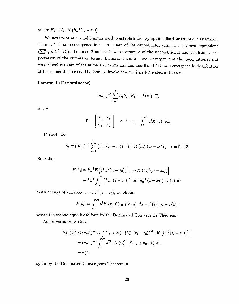
We next present several lemmas used to establish the asymptotic distribution of our estimator.

Lemma 1 shows convergence in mean square of the denominator term in the above expressions

(> ZZZ,' . K2). Lemmas 2 and 3 show convergence of the unconditional and conditional ex-

pectation of the numerator terms. Lemmas 4 and 5 show convergence of the unconditional and

conditional variance of the numerator terms and Lemmas 6 and 7 show convergence in distribution

of the numerator terms. The lemmas invoke assumptions 1-7 stated in the text.

Lemma 1 (Denominator)

(nh)1ZZ f(zo) •F,

where

r = 'Yo 'Yi and = f u1K (u) du.'Yi Y2

P roof. Let

O1(nhn)1(h1(zj_zo))l.Ij.K(h1(zj_zo)), 10,1,2.

Note that

E [Os] = h1E [(h1(z—

z0))' . I K (h'(zj — zo))]

=h1f (h'(z-zo))1 .K(h'(z_zo)) .f(z) dz.

With change of variables u = h;' (z — ZO), we obtain

E[Oi]__fuhK(u)f(zo+hnu) du=f(zo)1+o(1),

where the second equality follows by the Dominated Convergence Theorem.

As for variance, we have

Var (Os) < (nh'E [i (z > zo). (h'(zj — zo))21. K (h1(z —

z0))2]

=(nh)_1f u21 .K(u)2 •f(zo +h .z) du

=o(1)

again by the Dominated Convergence Theorem. U

26

We now consider the asymptotic behaviors of

(nh,)_l/2Zy* K and (nh)'/2Zx Ki.

For this purpose, define

(z) m (z) — a0 — b0 (z — ZO)— (zo) (z — zO)2

and e(z)p(z)_co_do(z_zo)_pF+(zo)(z_zo)2,

and observe that

sup K(z)I = o(h), sup (z)j =zo<z<zo+Mhn zo<z<zo+Mh,

where M is defined in Assumption 1.

Lemma 2 (Numerator: Expectation)

E[(nhfl)_1zv .K] f(zo)m"(zo)h•(6+o(1)),

E[(mhfl)_1zix: .K] f(zo)p" (zo)h'(+o(1)),

where

— fu2K(u)duf°u3K(u) du

P roof. We only prove the first claim because the second can be similarly established. Let

U1 = (nh)1 (h1(z — zo))1 I = 0,1.

Observe that

E [U1] = h1E [(h1(z — zo))1 (rn (z) — ao — (z — z0)) K]

=h'E [(hn'(zi — zo))1 (m" () . (z — zo)2 + ((zi))

.

Ki].Without loss of generality, we can assume that [—M, M] contains the support of K. We then have

E [U1] = (zO) .h_1f (h1 (z - zo)) (z - zo)2 K (h;' (z— zo)) 1(z) dz

+o(h).f (h1(z_zo))lK(h1(z_zo))f(z)dzfl ZO

27

We now note that

h;' f (h'(z - zo))l (z - zo)2K (h1 (z - zO)) 1(z) dz

= hf utu2K (u) f (zo + hu) du0

= f(zo)6ih+o(h),by the Dominated Convergence Theorem. We also note that, because

f u1K (u) f (z0 + hu)

is finite, we have

h' f (h1 (z — zo))1 K (h' (z — zo)) f (z) dz = f u1K (u) f (zo — hu) du

= 0(1).

.Lemma 3 (Numerator: Conditional Expectation)

(nh)' E [Zy K z] = E [(nh)_1 Zy K] + °p (h),

(nh)' E [Zx . K z] = E[(n)_1

Zx .

K]+ o (h).

P roof. Again, we only prove the first claim. We have

(nh)' E [Zy . K z] = (nh)1 ZK• (m(z) — ao — b0• (z — zo))

(nh)1+

(zo) (z — zo)2 + (zi))

Observe that

Var [(mhn)_1(ic1(zi _zo))1Kj. (mt'(zo) . (z_zo)2+(zi))]

= (nh'Var [(h1(z_zo))1K. (mu' (zO) . (z _zo)2+c(zi))]< (nh)'CE [(iç1(z2 — zo))21 K . ((zi

— zo) + ( (zi)2)]

=c .h4(nh2 ylhj u214.K(u)2.f(zo+h.u) du

+ C . o (h) (nh)1h f u21 . K (u)2 . f (zO + h . u) du

28

(The C after the inequality denotes a generic positive and finite constant.) By the DominatedConvergence Theorem, we have

Var [(nhY1 (h(z - zo))1K. (m' (ZO) (z — zo)2 +(z))]= 0 (n'h) + o (n1h)

h. [0 (m1h) + o (n')]=h.o(1).

The conclusion follows. •

Lemma 4 (Numerator: Conditional Variance)

Var [(nh)_1 (Zy K —E[Zy Kj

Fvo+o(1) vi+o(1) 1

=(nhn)2(zo)f(zo)[ V2+O(1)]

Var

[(nh)_1(Zx K — E [Zx K zi])]

r v+o(1) vi+o(1) 1= (nh)'p (zO) (1—p (zO)) f (zO) I

L vi+o(1) v2+o(1) ]

Coy[(nh)_1

(Zy . — E[Zy K z]) , (nh)1 (Zx K — E [Zx KI zi])]

F vo+o(1) vi+o(1) 1= (n)1(zo)f(zo)L vi+o(1) V2+O(1) ]

where'P00

VI = I u1K(u)2 du.Jo

P roof. Again, only the first claim is proved. Becausen

(nh)' (Zy . — E [Zy . K z])i=1

n= (nhy'ZK (y —a0 —b0 . (z —ZO) — (m(z) —a0 —b0 (z —

i=1n

= (nh)'ZK. (y —m(z)),i=1

29

we only consider

(nh)1 K• (h1 (z — zo))1 (y — m (z)), 1 = 0,1,2.

Notice that its variance equals

(nh)1E [K22 (h1(zj zo))21 a2 (z)]

(nh)_1f(h1(z_zo))21.K(h1(z_zo))2.a2(z) .f(z) dz

=(nh)_1fu21.K(u)2.a2(zo+h.u).f(zo+h.u)du

= (nh)' (2+ (zO)f (zo) vj + 0(1)).

The conclusion follows. •

Lemma 5 (Numerator: Conditional CLT)

(rih)112 ( Z . K — E [Zjy . KZx'.Kj—E[Zjx.KIz2]

f(zo)_1(0 a2+(z)S +(zo)Sp(zo)(l—p(zo))S )'

where

s= 0 V1V1 V2

P roof. We only consider

(nh)112 (Zy K — E [Zy . Kj z]).

By Cramér-Wold device, it suffices to establish that

g2 (zo) f(zo) . AsA ' (Zy K — E [Zy . K z]) (0, 1)

for every A E R2. For simplicity, we consider CLT term by term, and ignore joint distribution. So

we only consider

(nh)"2 K. (h'(zj — zo))1 (y— m (z)), 1 = 0,1.

30

We apply Lyapounov with third absolute moment: We need to establish

31

((flhn)_1U2+ f (zn) v21)-3/2

(nh)3 E [K. (h1(zj — ZO))— m (z) ] = o(1)

i=1or

31(nh "2h'E [K. (h1(zj — zo)) Iy — m(zj)131 = o(1).n)

Let

(z) E [Yi - m(z)J ;].Because

31h1E [Kr. (fç'(z — zo)) Iyi — m(zi)I]

=h1 / (h1(z_zo))3I.K(h1(z_zo))3. C (z).f(z) dzJ zo

'00= I u31 . K (u)3. ((zo + h u) f (zo + h u) du,

0

we have

31h1E [K. (h'(z — zo)) y — m (z)3] = 0(1)

and the conclusion follows.

Lemma 6 (Numerator: Unconditional CLT)

(nh)1"2 (Zy . K (nh)'/2h2

(m' (zo) 5 \

Zx•K )

—2 mf(zo)

p(z0). )/ r 2

zo)S ij(zo)Sf(zo)112 V O, [+()S p(zo)(1-p (zo))S])P roof. Due to Lemmas 2 and 3, we have

(flhfl)1/2EI(\

L )]=(nh)1/2hf(

/ m"(zo).(+o(1))(z0)(+o(1)) )

ZO)

and

E[

n

(ziY:.K\I1 n r/Z*K\\

flzjI =(y1/2E ((nh)'/2j1 Zx•K ) j [\Zjx.Kj)] +(nh)112o(h).

It follows that

E[(hY1/2

(Zy

K) zi]- '(n)1/2h2f (zo)

(

m' (z0) . (+ o(1)) \ o (nh).p(zo)(6+o(l)) )=i=1 \ Z2x K

The conclusion follows.

The following lemma gives the joint distribution for a—ao, h (' —bo) , —c and h (d_ do)

31

Lemma 7

(nh)'/2 (—ao, h (_bo), s—Co, h(d_do))'

= '(fl)1/2h2F 0 (m (zo) 6

2 0 F1 p(zo).5+f(zo)"2

F' 0 u(zo)S +(zo)S +o(1).0 F1 \ (zo)S p(zo)(1—p(zo))S J

P roof. Follows easily from Lemmas 1 and 6..

Proof of Theorem 1 and 1'As a consequence of lemmas 1-8, we obtain

( — Y m" +(zo) () + ()

+_+ ,/ p"(z) i(zo) p(zo)(1—p(zo))

Analogous expressions can be obtained for ( — y, — . Since observations are independent,

n — y, + — x±)' and n( — y, — are independent of each other. At this point,

the result stated in theorem 1 of the text follows straightforwardly by the Delta Method so the rest

of the proof is omitted. U

32

Data Appendix

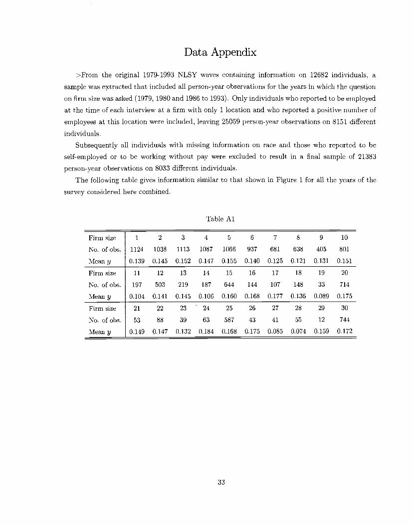
>From the original 1979-1993 NLSY waves containing information on 12682 individuals, a

sample was extracted that included all person-year observations for the years in which the question

on firm size was asked (1979, 1980 and 1986 to 1993). Only individuals who reported to be employed

at the time of each interview at a firm with only 1 location and who reported a positive number of

employees at this location were included, leaving 25059 person-year observations on 8151 different

individuals.

Subsequently all individuals with missing information on race and those who reported to be

self-employed or to be working without pay were excluded to result in a final sample of 21383

person-year observations on 8033 different individuals.

The following table gives information similar to that shown in Figure 1 for all the years of the

survey considered here combined.

Table Al

Firmsize

No. of obs.

Mean y

1 2 3 4 5 6 7 8 9 10

1124 1038 1113 1087 1066 937 681 638 405 801

0.139 0.145 0.152 0.147 0.155 0.140 0.125 0.121 0.131 0.151

Firm size

No. of obs.

Mean y

11 12 13 14 15 16 17 18 19 20

197 503 219 187 644 144 107 148 33 714

0.104 0.141 0.145 0.106 0.160 0.168 0.177 0.136 0.089 0.175Firm size

No. of obs.

Mean y

21 22 23 24 25 26 27 28 29 30

53 88 39 63 587 43 41 55 12 744

0.149 0.147 0.132 0.184 0.168 0.175 0.085 0.074 0.159 0.172

33

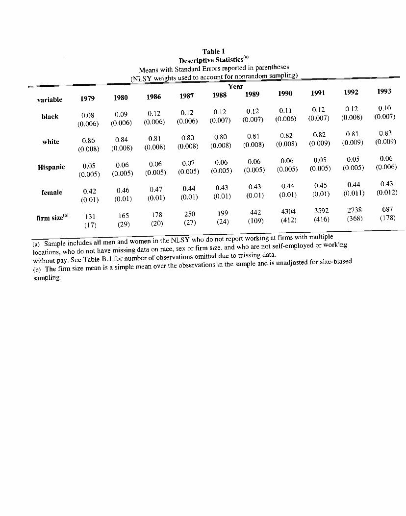
Table 1Descriptive Statistics

Means with Standard Errors reported in parentheses(NLSY weights used to account for nonrandom sampling)

Year

variable 1979 1980 1986 1987 1988 1989 1990 1991 1992 1993

black 0.08 0.09 0.12 0.12 0.12 0.12 0.11 0.12 0.12 0.10

(0.006) (0.006) (0.006) (0.006) (0.007) (0.007) (0.006) (0.007) (0.008) (0.007)

white 0.86 0.84 0.81 0.80 0.80 0.81 0.82 0.82 0.81 0.83

(0.008) (0.008) (0.008) (0.008) (0.008) (0.008) (0.008) (0.009) (0.009) (0.009)

Hispanic 0.05 0.06 0.06 0.07 0.06 0.06 0.06 0.05 0.05 0.06

(0.005) (0.005) (0.005) (0.005) (0.005) (0.005) (0.005) (0.005) (0.005) (0.006)

female 0.42 0.46 0.47 0.44 0.43 0.43 0.44 0.45 0.44 0.43

(0.01) (0.01) (0.01) (0.01) (0.01) (0.01) (0.01) (0.01) (0.011) (0.012)

firm size0 131 165 178 250 199 442 4304 3592 2738 687

(17) (29) (20) (27) (24) (109) (412) (416) (368) (178)

(a) Sample includes all men and women in the NLSY who do not report workingat firms with multiple

locations, who do not have missing data on race, sex or firm size, and who are not self-employedor working

without pay. See Table B.1 for number ofobservations omitted due to missing data.

(b) The firm size mean is a simple mean over the observations in the sample and is unadjusted for size-biased

sampling.

Table 2Estimated Effects of EEOC-reporting on Percentage Minority in the Firm

(asymptotic standard errors reported in parentheses)Year

Bandwidth 1979 1980 1986 1987 1988 1989 1990 1991 1992 1993

8 -8.7 -26.8 9.8 10.9 12.2 9.8 4.7 11.1 3.7 7.6(9.1) (11.3) (6.7) (5.3) (8.9) (11.1) (5.9) (4.1) (10.4) (9.1)

10 -2.1 -7.5 5.1 10.1 3.7 1.5 4.3 9.4 2.7 6.1(5.9) (9.0) (6.9) (4.6) (7.5) (6.0) (7.3) (4.6) (10.0) (8.8)

12 3.3 1.9 3.3 10.5 -1.3 5.5 7.4 9.6 2.6 4.7(4.5) (13.2) (8.7) (4.7) (8.3) (6.7) (9.0) (4.8) (12.0) (12.0)

14 8.2 8.8 1.9 10.6 -2.7 8.0 10.3 11.5 5.3 -1.5(5.4) (18.6) (11.2) (5.1) (8.0) (8.4) (8.8) (4.7) (13.8) (14.0)

globalIV 3.3 7,1 8.4 6.7 8.3 8.2 7.2 7.9 11.0 7.4(0.3) (0.4) (0.3) (0.3) (0.3) (0.3) (0.3) (0.4) (0.5) (0.4)

local IV with 0.92 3.03 2.8 4.0 3.7 3.8 2.6 3.0 3.5 -1.0bw=12 (0.3) (0.3) (0.2) (0.1) (0.3) (0.2) (0.2) (0.3) (0.3) (0.3)

(a) The first four rows report results from using the estimator based on local linear regressiondescribed in section 4.2 of the text. The last two rows report results using a global Waldestimator (i.e. one that uses all the data) and a local Wald estimator (one that only uses datawithin a bandwidth).

Table B.1Number of Observations Omitted

Year1979 1980 1986 1987 1988 1989 1990 1991 1992 1993

number of 1893 1935 2874 2962 2784 2788 2758 2395 2357 2313

observations

missingrace 11 15 12 19 13 10 13 15 18 16

missingclassof 0 0 339 372 411 507 441 466 499 528worker or self-employed or

working withoutpay

numberafter 1182 1935 2528 2575 2362 2275 2305 1918 1845 2297omitting personswith missing data

(a) The number of observations in the second row are all men and women in the NLSY who do notreporting at firms with multiple location. None of the observations were missing data on sex.

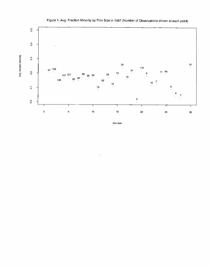
Figure 1: Avg. Fraction Minority by Firm Size in 1987 (Number of Observations shown at each point)

U,0

d

c 20 91

11010521 ii 640

74 6107 127 68 58 82 29

10138 83

621016

19 50 -

7

30 -0I I I

0 5 10 15 20 25 30

firm size

Table B.2Estimated Effects of EEOC-reporting on Percentage Minority in the Firm

omitting from the Sample Firms with Exactly 15 employees(asymptotic standard errors reported in parentheses)

Bandwidth 1979 1980 1986 1987Year

1988 1989 1990 1991 1992 1993

8 45.0(35.8)

-30.7(12.9)

31.2(18.9)

16.2

(10.8)5.1 8.8

(14.5) (24.9)-3.2(7.4)

-7.1

(6.8)5.8

(14.9)-3.6

(12.6)

10 15.0(14.0)

-7.7(9.2)

14.8

(10.4)14.0(5.2)

-6.6 1.1

(9.0) (7.8)0.7

(7.7)0.3

(0.5)5.0

(11.7)-3.5(9.3)

12 10.9(10.7)

3.4(13.3)

10.9

(10.7)13.4

(5.0)-12.3 5.3(8.9) (7.5)

6.2(9.4)

3.2(5.5)

2.3(12.9)

-2.8(12.1)

14 13.2

(9.9)11.3

(18.9)8.3

(12.4)13.1

(5.2)-12.9 7.9(8.2) (8.9)

10.3

(9.3)7.1

(5.5)4.4

(14.4)0.2

(14.1)

global IV 3.5(0.4)

7.5

(0.4)9.0

(0.3)6.9

(2.9)8.2 8.5

(0.4) (0.4)7.3

(0.4)0.8

(0.4)11.2

(0.5)8.1

(4.4)

locallVwithbw=12

1.3

(0.4)4.0

(0.4)4,2

(0.3)4.3

(0.1)1.3 4.0

(0.3) (0.2)2.4

(0.2)2.5

(0.3)4.4

(0.3)-0.0(0.4)

(a) The first four rows report results from using the estimator based on local linear regressiondescribed in section 4.2 of the text. The last two rows report results using a global Waldestimator (i.e. one that uses all the data) and a local Wald estimator (one that only uses datawithin a bandwidth).

00

0o c'JdE00(C 0(C

00

0C)d

. 0o c'j. dC00CC 0(C

00

0Cl0

o cjd

EC00CC 0CC

00

0Cl0

>'•C 0o c'jaEC00(C 0(C

q0

0Cl0

o C'J. dEC00(C 0

(C

q0

Figure 2: Estimated Percentage Minority Conditional on Firm Size (bw=12)

Year=1979 Year=1987

0 5 10 15 20 25 30

firm size

Year= 1980

00

0 5 10 15 20

firm size

Year= 1988

25 30

0 5 10 15 20 25 30

firm size

Year = 1989

0 5 10 15 20 25 30

firm size

Year= 1986

> 0

(C

000 5 10 15 20 25 30 0 5 10 15 20 25 30

firm size firm size

o csj

EC0C-)Cu 0Cu

0

00

>•0 0o c-'j. dEC00Cu 0Cu

q0

00

>•= 0o cj. 0EC0C.)Cu 0Cu

Figure 2: Estimated Percentage Minority Conditional on Firm Size (bw=12)

00

>'0o. d

EC0C.)Cu- 0Cu

00

Year= 1990 Year= 1993

0 5 10 15 20 25 30

firm size

P00 5 10 15 20 25 30

firm size

Year = 1991

0 5 10 15 20 25 30

firm size

Year= 1992

000 5 10 15 20 25 30

firm size