nber working paper series retirement policy and …
TRANSCRIPT
NBER WORKING PAPER SERIES
RETIREMENT POLICY AND ANNUITY MARKET EQUILIBRIA:EVIDENCE FROM CHILE
Gastón IllanesManisha Padi
Working Paper 26285http://www.nber.org/papers/w26285
NATIONAL BUREAU OF ECONOMIC RESEARCH1050 Massachusetts Avenue
Cambridge, MA 02138September 2019
A previous version of this paper was circulated as “Competition, Asymmetric Information, and the Annuity Puzzle: Evidence from a Government-run Exchange in Chile.” The research reported herein was performed pursuant to a grant from the U.S. Social Security Administration (SSA) funded as part of the Boston College Retirement Research Consortium. Padi acknowledges additional financial support from the Center for Equitable Growth and the National Science Foundation. The opinions and conclusions expressed are solely those of the authors and do not represent the opinions or policy of SSA, any agency of the federal government, or Boston College. The authors would like to thank Benjamin Vatter for outstanding research assistance, as well as Carlos Alvarado and Jorge Mastrangelo at the Superintendencia de Valores y Seguros and Paulina Granados and Claudio Palominos at the Superintendencia de Pensiones. We also thank Pilar Alcalde, Natalie Bachas, Vivek Bhattacharya, Ivan Canay, Liran Einav, Amy Finkelstein, Jerry Hausman, Igal Hendel, J.F. Houde, Koichiro Ito, Mauricio Larrain, Ariel Pakes, James Poterba, Mar Reguant, Nancy Rose, Casey Rothschild, Paulo Somaini, Salvador Valdes, Bernardita Vial and Michael Whinston for their useful comments, as well as numerous conference and seminar participants. The authors declare that they have no relevant or material financial interests that relate to the research described in this paper. The views expressed herein are those of the authors and do not necessarily reflect the views of the National Bureau of Economic Research.
NBER working papers are circulated for discussion and comment purposes. They have not been peer-reviewed or been subject to the review by the NBER Board of Directors that accompanies official NBER publications.
© 2019 by Gastón Illanes and Manisha Padi. All rights reserved. Short sections of text, not to exceed two paragraphs, may be quoted without explicit permission provided that full credit, including © notice, is given to the source.

Retirement Policy and Annuity Market Equilibria: Evidence from ChileGastón Illanes and Manisha PadiNBER Working Paper No. 26285September 2019JEL No. D15,D82,G22,G28,H31,H44
ABSTRACT
Retirement policy has indirect effects on its beneficiaries, through the “crowd-out” or “crowd-in” of insurance markets. We study how retirement policy in Chile, which limits the drawdown of retirement assets but otherwise does not provide or require fixed income in retirement, results in more than 60%of eligible retirees purchasing private annuities at low prices. We estimate a demand model to show that replacing this voluntary policy with partial mandatory annuitization and removing limits on drawdowns causes the private annuity market to partially unravel. Under our model, this reform leads to a welfare increase equivalent to US$4,000 of additional pension savings on average, but welfare effects are heterogenous and many retirees would be harmed due to the higher prices of private annuities. Our results highlight the importance of considering the impact of policy reforms on the equilibria of related markets.
Gastón IllanesDepartment of EconomicsNorthwestern UniversityKellogg Global Hub, Room 34212211 Campus DriveEvanston, IL 60208and [email protected]
Manisha PadiUC Berkeley225 Bancroft WayBerkeley, CA [email protected]
A data appendix is available at http://www.nber.org/data-appendix/w26285

Governments leverage several policy tools to provide financial security to their retirees. Some
publicly provide social insurance, while others require mandatory purchase of certain private in-
surance products.1 In the shadow of these policies, retirees will have different willingness to pay
for private insurance, and the risk of the privately insured population may change. Equilibrium
prices and transaction volumes in the private market will vary based on the government’s regula-
tory approach, resulting in ”crowd-in” or ”crowd-out” of private purchases. The welfare impact of
a policy, therefore, includes both its direct effect and its indirect effect on private market equilibria.
We study the relationship between private market outcomes and regulation in Chile, which
allows a choice between private market annuitization and a regulated drawdown path of retirement
savings. This voluntary policy requires neither mandatory purchase of private insurance nor does it
provide a default “public option,” providing a unique opportunity to observe active selection into a
robust private insurance market without mandates.2 In the shadow of Chile’s voluntary retirement
policy, we observe many retirees purchasing private annuities at low prices. Our project studies the
welfare of the entire distribution of retirees within this voluntary retirement system that crowds in
a robust private market, relative to counterfactual policies that crowd-out private annuity markets.
Annuities have the attractive feature of insuring against longevity risk by providing a fixed
income stream for the remainder of the annuitant’s lifetime. Moreover, they can accommodate
heterogeneous preferences across the retiree population by offering optional features such as guar-
anteed payments to the annuitant’s heirs or delaying payments until a later age. Because of this, the
previous literature has recognized this class of assets as potentially playing a central role in retire-
ment income portfolios. Despite the theoretical benefits of annuitization, most households in the
developed world choose not to purchase private market annuities. This phenomenon, often called
1A large literature explores the role of mandatory purchase of private insurance as an alternative or supplement tosocial insurance, including Crivelli, Filippini and Mosca (2006), Brown and Finkelstein (2008), Einav, Finkelstein andSchrimpf (2010), and Hackmann, Kolstad and Kowalski (2015).
2Some papers, including Rothschild (2009) and Hosseini (2015), study private insurance markets without anymandates or drawdown limits.
2

the “annuity puzzle”, has spurred a series of papers that attempts to explain retiree behavior.3
We explore an alternate explanation to the annuity puzzle - that mandatory public pension pro-
grams like Social Security crowd-out private annuity markets, while voluntary retirement policies
crowd-in private markets..4 To do so, we take advantage of the unique case study of Chile’s priva-
tized social security system. Using novel individual-level data on every annuity and programmed
withdrawal offer provided on this platform from 2004 to 2012, every choice made, and mortality
realizations until mid-2015, we document three key facts about the market for private annuities
in Chile. First, over 60% of retirees in Chile purchase a private annuity, meaning that Chile is
an exception to the annuity puzzle. Second, annuity prices are low: the average accepted annuity
is 3% less generous than the actuarially fair annuity. Third, through the Chiappori and Salanie
(2000) test for asymmetric information, we show that the Chilean equilibrium survives despite the
presence of adverse selection. That is, the equilibrium in this system features low prices and high
transaction volumes despite dealing with the same challenges facing most insurance markets.
We hypothesize that two features of the Chilean retirement policy drive crowd-in of the pri-
vate market - the lack of mandatory annuitization, and the limits placed on the outside option to
annuitization, namely drawdown of retirement assets. Since 2004, Chile has facilitated the sale
of private annuities through a government-run exchange which does not require any retirees to
purchase a fixed income product. The exchange is a virtual platform which transmits consumer in-
formation and preferences to all annuity providers (life insurance companies), solicits offers from
any company willing to sell to that consumer, and organizes the offers by generosity to facilitate the
retiree’s decision process. Retirees may also choose not to purchase an annuity and instead to draw
down the balance of their retirement savings account, according to a schedule set by the govern-
3Although this literature is very broad, some proposed explanations are adverse selection and high prices(Friedmanand Warshawsky (1990), Butler and Teppa (2007), Mitchell et al. (1999)), behavioral biases (Davidoff, Brown andDiamond (2005), Bernartzi and Thaler (2011), Brown et al. (2017)), bequest motives (Lockwood (2012)) and uncertainhealth expenditures (Reichling and Smetters (2015))
4This has previously been discussed in the theory literature, including Caliendo, Guo and Hosseini (2014).
3

ment. This alternative is called “programmed withdrawal”. Relative to annuitization, programmed
withdrawal allows retirees to leave more wealth for their heirs if they die early, and provides more
liquidity early in retirement. Therefore, it is more valuable as a vehicle for bequests and liquidity,
rather than as a source of insurance against longevity. In this setting, the government’s role is
primarily transmitting information between firms and consumers in the exchange, without limiting
price discrimination or constraining consumer and firm choice, and in designing the outside option
to annuitization.
We calibrate a life cycle model and calculate implied annuity demand and average cost curves
to demonstrate crowd-in and crowd-out under the current Chilean system and alternatives. Chile’s
retirement policy, including the design of programmed withdrawal and the lack of mandatory social
security, results in private market annuity demand that is relatively inelastic. In contrast, introduc-
ing mandatory partial annuitization at the actuarially fair rate and allowing retirees to allocate their
remaining savings between lump sum withdrawal and a private market annuity leads to more elas-
tic annuity demand. That means average cost increases faster than willingness to pay for annuities,
leading to a market with lower levels of annuitization. There are three main forces behind this
change: first, willingness to pay for each annuitized dollar mechanically decreases for the whole
population when a significant fraction of wealth is pre-annuitized, and as a result demand contracts;
second, this effect is heterogenous across retirees, depending on their underlying preferences for
financial instruments, so that demand rotates; and third, these reforms can affect which individuals
annuitize at a given annuity payout, and how much they annuitize, so that the average cost curve
shifts. Additionally, the calibration also demonstrates two important features of the setting that
motivate our econometric model. First, that the relationship between mortality and other drivers of
preferences for financial instruments, such as bequest motives and risk aversion, can greatly affect
annuity market equilibria.5 Second, that average cost and demand are non-linear, and as a result
linear approximations to these objects will be inaccurate for large-scale counterfactuals, such as5Building on work such as Finkelstein and McGarry (2006) and Einav, Finkelstein and Schrimpf (2010).
4

the ones we are interested in studying.
To quantify the impact of changes in retirement policy on private market equilibria, we estimate
a structural model that traces out the demand curve for annuities in Chile. Our model allows us
to nonparametrically estimate the distribution of private information in the market. The model
proceeds in two steps. First, we discretize the space of unobserved heterogeneity and solve an
optimal consumption-savings problem to value every annuity and programmed withdrawal offer
for every combination of unobserved heterogeneity or type. We then use the estimator presented in
Fox et al. (2011) and Fox, il Kim and Yang (2016) to non-parametrically estimate the distribution
of types that rationalizes observed choices. The main advantage of this approach relative to other
demand estimation techniques is that our consumption-savings model allows us to value out-of-
sample financial contracts and to predict choices type-by-type, while the estimated distribution
of types allows us to aggregate and predict private market equilibria. We then calculate welfare
changes for each consumer type taking into account equilibrium price responses.
Demand estimates highlight that there is significant unobserved heterogeneity among retirees,
even after conditioning on observables. Moreover, we find evidence of correlations across dimen-
sions of unobserved heterogeneity. Using the estimated distribution of unobserved types, we show
that the design of the Chilean retirement system does in fact crowd-in the private market, since
moving to counterfactual retirement policies leads to lower annuitization rates and higher prices.
First, we simply increase the value of the outside option for every type of retiree by removing lim-
its on retirement savings drawdown. This crowds out the private market by lowering willingness to
pay for private annuities, resulting in lower transaction volume and higher prices. Having access
to a better outside option therefore lowers the welfare of those who continue to purchase private
annuities. Although the average welfare change is positive, we find that 45% of retirees have lower
welfare from this reform due to the equilibrium response of the private annuity market.
More significant crowd-out is observed when retirement policy includes mandatory retirement
5

income, similar to publicly provided Social Security or mandatory purchases of private annuities
as in the UK. Moving to a mandatory policy further lowers willingness to pay for additional an-
nuitized wealth, causing significantly higher private annuity prices and a larger drop in annuitized
wealth. Under this counterfactual policy regime, we can generate the same low annuitization lev-
els described in the annuity puzzle literature. Despite this, we find that on average retirees would
experience a welfare increase equivalent to an additional $4,000 dollars of pension savings under
this reform. This average masks substantial heterogeneity and redistribution across dimensions
of unobserved type. A crowded-out private annuity market in the presence of mandatory public
retirement policy significantly lowers welfare for about 25% of retirees, but it does generate higher
welfare for a majority of our population.
Related Literature
This work brings together two strands of the literature. The first is the literature on crowdout
and the interaction between public policy and private markets. Starting with Cutler and Gruber
(1996), researchers have documented how public spending crowds out private insurance. Examples
include unemployment benefits (Cullen and Gruber (2000)), public health insurance (Cutler and
Gruber (1996), Sloan and Norton (1997), Gruber and Simon (2008)), long term care insurance
(Brown, Coe and Finkelstein (2007), Brown and Finkelstein (2008)), and emergency care and
bankruptcy (Koch (2014), Mahoney (2015), Garthwaite, Gross and Notowidigdo (2018)). This
work generally shows that public policy can impact private markets, but stops short of modeling
and estimating private market primitives and therefore cannot compute welfare effects of large
scale policy reforms. Hosseini (2015) and Caliendo, Guo and Hosseini (2014) uses calibrated
theory models to demonstrate the potential impact of retirement policy in private annuity markets.
We connect this literature to the second strand of scholarship, modeling and estimating equi-
6
librium in markets with asymmetric information using data on insurance purchases. We start with
a structural model to back out the distribution of retirees’ private information, based on Einav,
Finkelstein and Schrimpf (2010). We take a more primitive approach to modeling demand than
other papers on publicly supported private insurance markets, including Medigap (Bundorf and
Simon (2006), Starc (2014), Keane and Stavrunova (2016)) and state health insurance exchanges
(Finkelstein, Hendren and Shepard (2017), Einav, Finkelstein and Tebaldi (2019) Tebaldi (2019)).
To this literature we add heterogeneity in risk preference and outside wealth. Our contribution is
to nonparametrically identify private information without making any assumptions on firm pric-
ing behavior. We also solve for counterfactual equilibria when significant changes are made to
retirement policy, and when the product set changes, accounting for equilibrium effects.
The rest of the paper is structured as follows: section 1 introduces the main features of the
Chilean retirement exchange; section 2 presents descriptive evidence on the functioning of this
system; section 3 develops the lifecycle model of consumption and savings used for both calibra-
tions and demand estimation; section 4 uses a calibration to show how differences in regulation
shift demand and average cost functions even with the same primitives; section 5 presents our
demand estimation framework, provides details on the empirical implementation, and discusses
identification; section 6 estimates the distribution of underlying types and uses demand estimates to
simulate counterfactual annuity market equilibria and welfare under different regulatory regimes;
and section 7 concludes.
1 The Chilean Retirement Exchange
Chile has a privatized pension savings system. Individuals who are employed in the formal
sector must contribute 10% of their income to a private retirement savings account administered
by a Pension Fund Administrator (PFA). In order to access the accumulated balance upon retire-
7
ment, retirees must utilize a government-run exchange called “SCOMP”6. The exchange can be
accessed either through an intermediary, such as an insurance sales agent or financial advisor, or
directly by the individual at a pension fund administrator. Individuals can enter SCOMP at any
time after they have accumulated more wealth than a legal minimum. In practice, since the mini-
mum wealth requirement falls significantly after certain age thresholds (60 for women and 65 for
men), most retirees enter the exchange at that point or after. Individuals provide the exchange with
their demographic information, private savings account balance, and the types of annuity contracts
they want to elicit offers for (choices are deferral of payments, purchase of a guarantee period to
provide payouts after death, fraction of total wealth to annuitize7, and transitory rents, an annuity
with a front-loaded step function).
There are between 13 and 15 firms participating in this exchange between 2004 and 2013. Once
an individual enters the exchange, each firm simultaneously receives the following information:
gender, age, marital status, age of the spouse, number and age of legal beneficiaries other than the
spouse, pension account balance, and the set of contracts for which offers have been requested.8
Armed with this information, each firm sets individual and contract type specific offers. They
can also not bid on some or all of the contracts the individual requested. There is no regulation
impeding price discrimination based on any of the characteristics firms observe through SCOMP.
There is, however, the requirement that all bids be denominated in an inflation indexed unit of
account (Shiller (1998)) called “Unidad de Fomento” (UF), so all annuities in this setting are
measured in real currency.9
Retirees can opt not to accept an annuity offer, but instead to take an alternative product, called
programmed withdrawal (“PW”)10. Programmed withdrawal provides a front-loaded drawdown of6Sistema de Consultas y Ofertas de Montos de Pension.7With significant restrictions. In our sample, fewer than 10% of retirees were eligible to not annuitize their total
savings8Other beneficiaries include children under 18 (25 if they are attending college)9In December 12, 2017, a UF was worth 40.85 USD
10All individuals who accept PW are still included in our sample.
8

Figure 1: A simulated path of payments made under PW to a retiree who retires at 60, comparedto the average annuity that retiree is offered
pension account funds according to a regulated schedule, with two key provisions. First, whenever
the retiree dies, the remaining balance in their savings account is given to their heirs. Second, if the
retiree is sufficiently poor and lives long enough for payments to fall below a minimum pension,
the government will top up PW payments to reach this minimum level.11 When an individual
chooses the PW option, their retirement balance remains at a PFA, which invests it in a low risk
fund. As a result, PW payments are stochastic, although the variance is small. Figure 1 shows one
realization of PW payments for a female who retires at 60, and compares it to the average annuity
offer that individual received.
Retirees receive all annuity offers and information about PW on an informational document
provided by SCOMP. The document begins with a description of programmed withdrawal and a
11The threshold for receiving the minimum pension is being below the 60% percentile of total wealth according tothe “Puntaje de Focalizacion Previsional”
9

Figure 2: Sample printout of programmed withdrawal information conveyed to retiree
sample drawdown path (figure 2). Then, annuity offers are listed, ranked within contract type first
by generosity (figure 3). Along with the life insurance company’s name, retirees are also informed
of their risk rating. This information is relevant, as retirees are only partially insured against the
life insurance company going bankrupt.12
After receiving this document, retirees can accept an offer or enter a bargaining stage. Retirees
can physically travel to any subset of firms that gave them offers through SCOMP to bargain for
a better price, for some or all of the contracts they are interested in.13 On average, these outside
offers represent a modest increase in generosity over offers received within SCOMP, on the order of
2%. Finally, the individual can choose either to buy an annuity from the final choice set or to take
PW. Individuals that don’t have enough retirement wealth to fund an annuity above a minimum
threshold amount per month will receive no offers from firms, and must take PW.
12To be precise, the government fully reinsures the MPG plus 75% of the difference between the annuity paymentand the MPG, up to a cap of 45 UFs. In practice, there has been only one bankruptcy since the private retirementsystem’s introduction in the 1980s, and that company’s annuitants received their full annuity payments for 124 monthsafter bankruptcy was declared. Only after that period did their payments fall to the governmental guarantee. Alcaldeand Vial (2017) study willingness-to-pay for different product attributes, including risk rating, finding that individualsare on average willing to give up around 1% of the offer value to accept an offer from a AA+ or better rated firm.
13Firms are not allowed to lower their offers in this stage
10

Figure 3: Sample printout of annuity offers for one contract type
Our primary source of data is the individual-level administrative dataset from SCOMP from
2004 to 2013, which includes the retiree’s date of birth, gender, geographic location, wealth, and
beneficiaries. This data includes contract-level information about prices, contract characteristics
and firm identifiers. We observe the contract each retiree chooses, including if they choose not to
annuitize, and can compare the characteristics of the chosen contract to the other choices they had,
including offers received during the bargaining stage. Overall, we observe 230,000 retirees and
around 30 million annuity offers. We supplement this data with two external datasets. First, we
include external data about the life insurance companies making offers, such as their risk rating14.
Second, we merge individual-level death records obtained from the Registro Civil in mid 2015.
Throughout our sample period, annuity contracts for married males are regulated to be joint
life annuities, while this is only the case for married females after 2007. Furthermore, for retirees
with children younger than 18, life insurance companies must continue paying out a fraction of the
annuity payment upon the retirees’ death until the child turns 18.15 For ease of calculation, we will
focus our analysis on the subsample of retirees with no beneficiaries. This subsample purchases14While this variable is presented to retirees, it was not made available to us directly in the SCOMP dataset.15Children younger than 25 are also covered if they are in college, until either they graduate or turn 25.
11
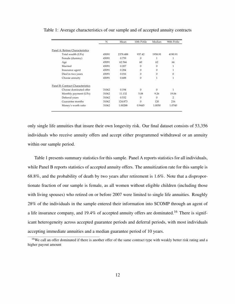
Table 1: Average characteristics of our sample and of accepted annuity contracts
N Mean 10th Pctile Median 90th Pctile
Panel A: Retiree CharacteristicsTotal wealth (UFs) 45091 2378.488 937.42 1958.91 4190.91Female (dummy) 45091 0.759 0 1 1Age 45091 62.566 60 62 66Married 45091 0.207 0 0 1Insurance agent 45091 0.284 0 0 1Died in two years 45091 0.016 0 0 0Choose annuity 45091 0.688 0 1 1
Panel B: Contract CharacteristicsChoose dominated offer 31062 0.194 0 0 1Monthly payment (UFs) 31062 11.132 5.08 9.26 19.06Deferral years 31062 0.532 0 0 2Guarantee months 31062 124.873 0 120 216Money's worth ratio 31062 1.00288 0.9445 1.0050 1.0740
only single life annuities that insure their own longevity risk. Our final dataset consists of 53,356
individuals who receive annuity offers and accept either programmed withdrawal or an annuity
within our sample period.
Table 1 presents summary statistics for this sample. Panel A reports statistics for all individuals,
while Panel B reports statistics of accepted annuity offers. The annuitization rate for this sample is
68.8%, and the probability of death by two years after retirement is 1.6%. Note that a dispropor-
tionate fraction of our sample is female, as all women without eligible children (including those
with living spouses) who retired on or before 2007 were limited to single life annuities. Roughly
28% of the individuals in the sample entered their information into SCOMP through an agent of
a life insurance company, and 19.4% of accepted annuity offers are dominated.16 There is signif-
icant heterogeneity across accepted guarantee periods and deferral periods, with most individuals
accepting immediate annuities and a median guarantee period of 10 years.
16We call an offer dominated if there is another offer of the same contract type with weakly better risk rating and ahigher payout amount
12
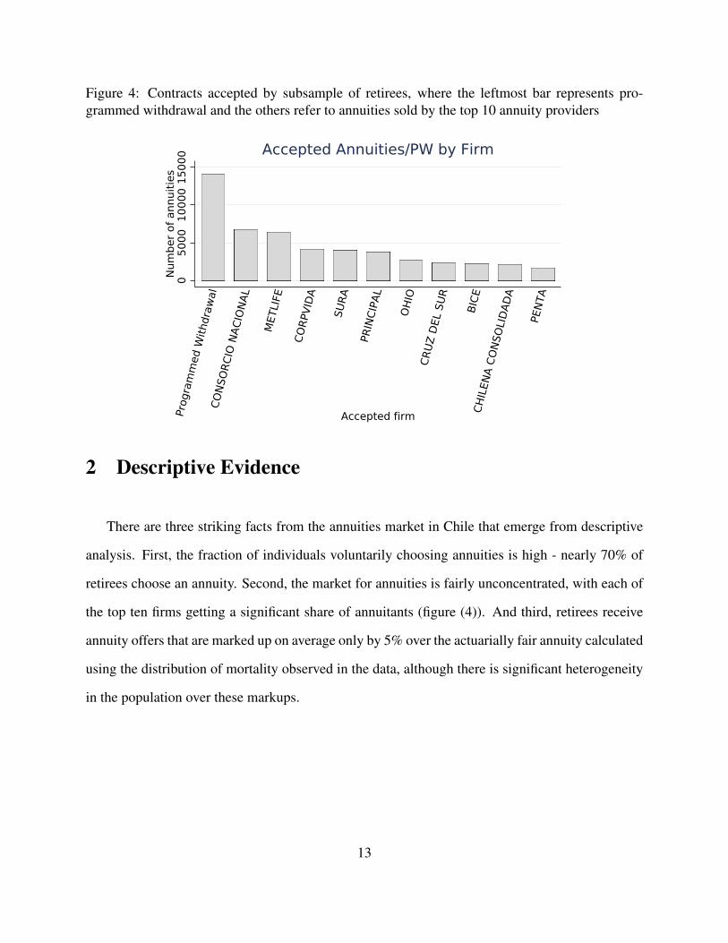
Figure 4: Contracts accepted by subsample of retirees, where the leftmost bar represents pro-grammed withdrawal and the others refer to annuities sold by the top 10 annuity providers
050
0010
000
1500
0N
umbe
r of a
nnui
ties
Prog
ram
med
With
draw
alCO
NSO
RCIO
NAC
IONA
L
MET
LIFE
CORP
VID
A
SURA
PRIN
CIPA
L
OHI
OCR
UZ D
EL S
UR
BICE
CHIL
ENA
CONS
OLI
DAD
A
PENT
A
Accepted firm
Accepted Annuities/PW by Firm
2 Descriptive Evidence
There are three striking facts from the annuities market in Chile that emerge from descriptive
analysis. First, the fraction of individuals voluntarily choosing annuities is high - nearly 70% of
retirees choose an annuity. Second, the market for annuities is fairly unconcentrated, with each of
the top ten firms getting a significant share of annuitants (figure (4)). And third, retirees receive
annuity offers that are marked up on average only by 5% over the actuarially fair annuity calculated
using the distribution of mortality observed in the data, although there is significant heterogeneity
in the population over these markups.
13

Calculating Annuity Value
We calculate actuarially fair annuities by modelling the hazard rate of death (h j(t)) as a Gom-
pertz distribution with a different scale parameter for each demographic type j (bins of age, gender,
municipality, and wealth level). The shape parameter γ is fixed and the scale parameter is modeled
as λ j = ex jβ . The resulting hazard rate is given by:
h j(t) = λ jeγt
Since we observe death before 2015, we can estimate this model directly for our sample. Using
the results of this estimation, we can predict expected mortality probabilities for each individual
and calculate the net present cost of an annuity with a monthly payout zt , discounted at rate r. The
predicted survival probabilities (dependent on age, gender, wealth, and municipality) are denoted
as {πit}. The NPV of an annuity can then be calculated as:
NPV (zi) =T
∑t=0
πitzi
(1+ r)t
Naturally, the value of the annuity payout depends on the total retirement savings the retiree gives
the life insurance company (denoted by wi). We calculate percentage markup over cost as:
mi =wi−NPV (zt)
NPV (zt)=
1MWRi
−1
A first pass at comparing the value of annuities relative to PW is to repeat the exercise done
in prior literature, which solves for the ratio of offered annuity NPV to the total amount of wealth
transferred to the insurance company. This amount is the money’s worth ratio (“MWR”). Mitchell
et al. (1999) perform this calculation for US retirees without a bequest motive facing actuarially
14

fair annuities, and find an MWR of between 0.82 and 0.92.17 We find that in our context, offered
annuities have a markup of about 5% over actuarially fair, which translates to a MWR of 0.952.
Accepted annuities have a markup of about 3% over actuarially fair, or a MWR of 0.97. Prices in
the Chilean market are therefore significantly lower than in other countries.
Selection
Though the market appears to be functioning remarkably well, there is significant adverse
selection in annuity purchase. To demonstrate this, we run the standard positive correlation test,
introduced by Chiappori and Salanie (2000). In our implementation of this test, we regress the
probability the retiree dies within two years of retirement, regressed on a dummy for annuity
choice. Table 2 shows this baseline correlation in column 1. Columns 2 and 3 check the robustness
of the result after controlling for observable characteristics of the individual and the requests the
individual makes for annuity offers. This is the full set of information life insurance companies
receive about retirees. We use the estimating equation:
ddeath,i = γannuitizedannuitize,i +X ′ΠD
Covariates X include all characteristics that firms may price on. The purpose of including
controls is to make sure that selection is on unobservable characteristics - selection on observable
characteristics can be reflected by a change in price, while selection on unobservables cannot be.
A negative correlation means that retirees buying annuities are less likely to die than retirees that
choose programmed withdrawal. Results show that annuitants are significantly more long lived
than those choosing programmed withdrawal, even conditional on characteristics that firms can
17We consider the before-tax values in their calculation for policies offered to men aged 65, which would be moregenerous than our population, where the modal annuitant is a 60 year old female.
15

Table 2: Chiappori & Salanie positive correlation test
(1) (2) (3)Death by 2 yrs Death by 2 yrs Death by 2 yrs
Choose annuity -0.00740** -0.00399** -0.00434**(0.00137) (0.00137) (0.00156)
Individual characteristics
Request characteristics
Observations 45091 45091 45091
Base group mean 0.015(0.121)
price on. To put this number in context, we run the correlation test using a Gompertz hazard model
(reported in figure 16 in Appendix C). From this, we can estimate the relative life expectancies
of annuitants, separately from non-annuitants. For a modal population of female retirees in 2010,
retiring without help from an intermediary, we estimate that annuitants live on average 7 months
longer than non-annuitants.
Despite the standard concerns regarding adverse selection, Chile’s regulatory regime supports
the existence of a healthy voluntary annuity market. Our goal is to estimate the primitives gov-
erning demand for these products, and to then simulate how reforming the Chilean regulatory
framework to make it more similar to the US shifts the market equilibrium. The following section
introduces the model we will use to value each contract.
3 Model
This section develops a model to value annuity and programmed withdrawal offers given a
vector of individual characteristics and unobserved preferences. In section 5, we will embed the
model into a discrete choice demand system to obtain estimates of unobserved preferences, and
use these estimates to evaluate counterfactuals where we change the regulatory environment. The
16

primary contribution of this model is to account for multiple dimensions of retiree private infor-
mation, allowing preferences to be far more heterogeneous than in prior work. Specifically, the
model allows for private information about mortality risk, bequest motives, risk aversion, and total
wealth.
Since individuals are making choices over financial instruments that differentially shift money
over time, change exposure to longevity risk, and vary the assets that are bequeathed upon death,
a suitable model needs to capture these salient features. In particular, we use a finite-horizon
consumption-savings model with mortality and bankuptcy risk and the potential for utility derived
from inheritors’ consumption. Consider the problem of a particular individual who faces a set of
annuity and programmed withdrawal offers. To obtain the value of each offer, the individual needs
to solve for the optimal state-contingent consumption path, taking into account uncertainty about
their own lifespan and about the probability that each life insurance firm will go bankrupt.
Before introducing the individual’s optimization problem, some additional notation is needed.
Fix an individual and firm, so we can suppress those subscripts. Let t = 0 denote the moment in
time when the individual retires, and let T denote the terminal period in our finite horizon problem.
Let ω denote outside wealth (the amount of assets held outside the pension system), γ denote
risk aversion, and δ denote the discount factor. Let dt = {0,1} denote whether the individual
is alive (0) or dead (1) in period t, and {µτ}Tτ=1 denote the vector of mortality probabilities 18.
Following Carroll (2011), let ct denote consumption in period t, mt the level of resources available
for consumption in t, at the remaining assets after t ends, and bt+1 the “bank balance” in t +1.
For the purposes of specifying the optimal consumption-savings problem given an annuity
offer, we also need to define qt , which denotes whether the firm is bankrupt (1) or not (0) in period
t, and the vector of bankruptcy probabilities for the offering firm {ψ j,τ}Tτ=1
19. With these objects,
18Clearly, d0 = 0 and µ0 = 019Naturally q0 = 0 and ψ0 = 0
17

we can write the annuity payment in period t conditional on dt , qt , the deferral period D and the
guarantee period G as zt(dt ,qt ,D,G).
With this notation, and suppressing individual and firm subscripts, we can write the individual’s
optimal consumption problem given an annuity offer as:
maxE0
[T
∑τ=0
δτu(cτ ,dτ)
]
s.t.
at = mt− ct ∀t bt+1 = at ·R ∀t
mt+1 = bt+1 + zt+1(dt+1,qt+1,D,G) ∀t at ≥ 0 ∀t
Where R = 1+ r, and r is the real interest rate, which we assume is deterministic and fixed over
time.20 Note that we are imposing a no borrowing constraint: there can be no negative end of period
asset holdings. This assumption greatly simplifies the problem from a computational perspective.
In practice, life insurance companies can offer loans against their annuity payments, but only do
so for five year terms and at interest rates exceeding 20%, so we do not believe this assumption to
be too restrictive. 21
20Annuity and PW offers in Chile are expressed in UFs, an inflation-adjusted currency, so everything in the modelis in real terms.
21It is also increasingly difficult to keep a checking account, credit cards, and home loans open as individualsage. For example, see (in Spanish) http://www.emol.com/noticias/Nacional/2018/07/04/912082/Pinera-anuncia-que-terminara-con-discriminacion-por-edad-en-servicios-bancarios-que-afecta-a-adultos-mayores.html
18

The exogenous variables evolve as follows:
m0 = ω, d0 = 0, q0 = 0
dt+1 =
0 with probability (1−µt+1) if dt = 0
1 with probability µt+1 if dt = 0
1 if dt = 1
qt+1 =
0 with probability (1−ψt+1) if qt = 0
1 with probability ψt+1 if qt = 0
1 if qt = 1
zt(dt ,qt ,D,G) =
z if qt = 0 and ((dt = 0 and t ≥ D) or (dt = 1 and D≤ t < G+D))
ρ(z, t) · z if qt = 1 and ((dt = 0 and t ≥ D) or (dt = 1 and D≤ t < G+D))
0 otherwise
Where ρ(z, t) is the annuity payment when the firm goes bankrupt:
ρ(z, t) =
MPGt if z≤MPGt
MPGt +min((z−MPG)∗0.75,45) if z > MPG
and MPG is the minimum pension guarantee. For the purposes of this model, we will assume that
the MPG is fixed over time. Assume that the utility derived from consumption when alive is given
by the following CRRA utility function:
u(ct ,dt = 0) =c1−γ
t
1− γ
19
whereas if the individual dies at the beginning of period t, her terminal utility at t is given by
evaluating the CRRA at the expected value of remaining wealth:
u(dt = 1) = β ·(mt +E[∑G
τ=t+1 δ t−τzτ(1,qτ ,D,G)])1−γ
1− γ
and is equal to zero thereafter.22
To obtain the value of an annuity offer, which is the present discounted value of the expected
utility of the optimal state-contingent consumption path, we solve this problem by backward in-
duction. At the terminal period, the problem is simple and has an analytic solution, but for periods
earlier than T it must be solved numerically. We use the Endogenous Gridpoint Method (EGM)
(Carroll (2006)) to solve this problem, obtaining V A(0,0;π), the present discounted value of the
expected utility of consumption obtained from following the optimal state-contingent policy path
given an annuity offer and the vector π of parameters23. See Appendix D for the full derivation of
the Euler equations and the computational details of the numerical solution.
Valuing a programmed withdrawal (PW) offer requires solving a slightly different problem. In
this setting there is no deferral or guarantee period, or bankruptcy risk for the asset. Furthermore,
inheritors automatically receive all remaining balances as a bequest upon death. All of these factors
simplify the problem relative to the annuity problem. Taking these differences into account, the
individual’s PW optimization problem, which gives us the value of accepting a PW offer from firm
22This assumption implies that individuals are not risk averse about the remaining uncertainty after death. If theywere, we would need to calculate expected utility instead of the utility of the expectation. From a practical perspective,this is unlikely to matter much, as the only case where remaining wealth is stochastic is for annuity offers with aguarantee period from firms who have not gone bankrupt, as wealth left to inheritors in this case is still subject tobankruptcy risk. Since bankruptcy risk is small, and most deaths will occur after the guarantee period expires, we arecomfortable making this assumption.
23Outside wealth ω , bequest motive β , mortality probabilities {µ}Tt=1, risk aversion γ , and bankruptcy probabilities
{ψ}Tt=1
20
a, is:
maxE0
[T
∑τ=0
δτu(ct ,dt)
]
s.t.
at = mt− ct ∀t bt+1 = at ·Rt+1∀t
mt+1 = bt+1 + zt+1(PWt+1,dt+1, f )∀t at ≥ 0∀t
where zt(PWt ,dt , f ) denotes the programmed withdrawal payout in period t conditional on pension
balance PWt , death status, and f , the commission rate charged by the firm. The death state and
initial conditions are as before, and the remaining exogenous variables evolve as follows:
zt(PWt ,dt ,a) =
max[zt(PWt) · (1− f ),MPG] if dt = 0
0 if dt = 1
PWt+1 = (PWt− zt(PWt)) ·RPWt
The PW payout function zt(PWt) is described in detail in Appendix A. All PFAs are governed
by the same PW function, and conditional on the PW balance, will pay out the same amount up
before the commission f . As a result, if PFAs provided the same returns over time, the amount
of money that is withdrawn every year from the PW account would be the same across PFAs, and
only how that money is distributed between the retiree and the PFA would vary across companies.
We will assume that in fact PFAs provide the same returns on PW investments, as this simplifies
the problem and is not far from reality, where PFA returns vary slightly for the safe investment
portfolios where PW balances are invested 24. Let RPWt be the return to programmed withdrawal
investments. Finally, MPG is the minimum pension guarantee. Every individual who takes PW
is guaranteed a payout of at least MPG, and the difference between zt(PWt) and MPG (when24Illanes (2019) documents this in detail
21

zt(PWt) < MPG) is funded by the government. Finally, utility derived from consumption is as
before, while upon death utility is:
u(dt = 1) = β · (mt +PWt)1−γ
1− γ
As for annuities, we solve this problem numerically by backwards induction using EGM, and ob-
tain V PW (0,PW0;π), the present discounted value of the expected utility of consumption obtained
from following the optimal state-contingent policy path given an initial PW balance of PW0 and
the vector π of parameters. See Appendix D for the full derivation of the Euler equations and the
computational details of the numerical solution.
4 Calibration
In this section, we calibrate the previous life cycle model and calculate the value of annuities
and programmed withdrawal for different distributions of preferences for financial instruments.
Given a distribution of preferences, we can map these utilities to a model of market equilibrium by
calculating annuity demand and average cost. Additionally, we can alter the rules governing how
individuals access their retirement savings, recalulate utilities, and study how the annuity market
equilibrium changes.
Below, we focus on a 60 year old female, retiring in 2007 with relatively high pension sav-
ings.25 We model heterogeneity in mortality risk as normally distributed shifts over the mortality
tables used by the Chilean pension authorities26. More precisely, given a retiree’s age, these tables
give us a mortality probability vector. We introduce heterogeneity as shifts in the individuals’ age,
so that a 65 year old retiree with a x year mortality shifter has the mortality probability vector
25At the third quartile of pension savings for women in our data26Superintendencia de Pensiones and Superintendencia de Valores y Seguros
22

of a 65+ x year old. This allows us to introduce unobserved heterogeneity in mortality risk in
a parsimonious way, at the cost of assuming that all shifts in mortality preserve the shape of the
regulatory agencies’ tables27.
In the baseline case, all other parameters in the model will be held fixed, so that the only source
of unobserved heterogeneity is mortality. Parameters of the utility function are taken from previ-
ous literature when possible.28 The risk aversion parameter is 3, interest rate is 3.18% (yearly), the
mean and standard deviation of the mortality shifter are 0 and 10, the bequest motive parameter
is 1, and 20% of the retiree’s total wealth that is in pension savings.29 To illustrate how correla-
tion across dimensions of unobserved heterogeneity can affect annuity market equilibria, we will
also present results where we keep the previous means but add positive correlation between the
mortality shifter and bequest motive, and negative correlation between this shifter and both outside
wealth and risk aversion.
We model retirees as choosing to allocate their pensions savings dollar-for-dollar between pro-
grammed withdrawal and a simple annuity with no deferral or guarantee period. We are abstracting
away from heterogeneity in preferences for contracts and preferences for firms, in order to focus
on how the demand function changes across institutional regimes.
To calculate the annuity demand function, we take a grid over the space of yearly annuity
payouts (expressed as a percentage of the pension balance) and calculate, for every type and pay-
out combination, the optimal allocation of pension balance between the annuity and programmed
withdrawal. This yields a vector of fractions of wealth annuitized for each level of annuity payout.
To obtain the aggregate fraction of wealth annuitized, or quantity demanded, we integrate over the
distribution of mortality shifters. To obtain the average cost of the annuitant population, we first
27These tables are specifically designed to capture the mortality expectations of the retiring population.28Our parameters for risk aversion, interest rates, bequests and outside wealth match or lie in the range discussed
by Hosseini (2015), as well as Einav, Finkelstein and Schrimpf (2010) and Lockwood (2012).29Wealth in the pension system is 3040 UFs, and outside wealth is 12160 UFs
23
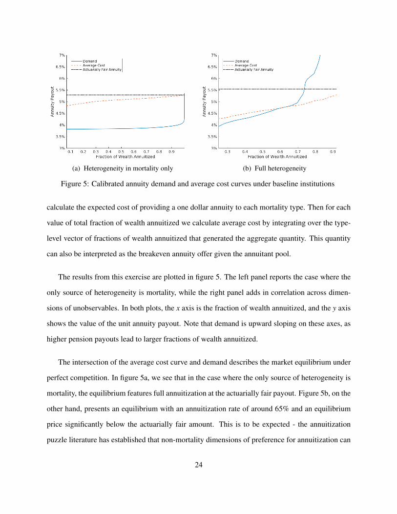
(a) Heterogeneity in mortality only (b) Full heterogeneity
Figure 5: Calibrated annuity demand and average cost curves under baseline institutions
calculate the expected cost of providing a one dollar annuity to each mortality type. Then for each
value of total fraction of wealth annuitized we calculate average cost by integrating over the type-
level vector of fractions of wealth annuitized that generated the aggregate quantity. This quantity
can also be interpreted as the breakeven annuity offer given the annuitant pool.
The results from this exercise are plotted in figure 5. The left panel reports the case where the
only source of heterogeneity is mortality, while the right panel adds in correlation across dimen-
sions of unobservables. In both plots, the x axis is the fraction of wealth annuitized, and the y axis
shows the value of the unit annuity payout. Note that demand is upward sloping on these axes, as
higher pension payouts lead to larger fractions of wealth annuitized.
The intersection of the average cost curve and demand describes the market equilibrium under
perfect competition. In figure 5a, we see that in the case where the only source of heterogeneity is
mortality, the equilibrium features full annuitization at the actuarially fair payout. Figure 5b, on the
other hand, presents an equilibrium with an annuitization rate of around 65% and an equilibrium
price significantly below the actuarially fair amount. This is to be expected - the annuitization
puzzle literature has established that non-mortality dimensions of preference for annuitization can
24

(a) Heterogeneity in mortality only (b) Full heterogeneity
Figure 6: Calibrated annuity demand and average cost curves under reformed institutions
lead to equilibria with less than full annuitization (for example, Lockwood (2012)).
Let us now consider the effects of imposing annuitization of a fraction of pension savings and of
allowing for lump sum withdrawal of the remainder. We follow Mitchell et al. (1999)) and impose
annuitization of one half of pension balances, only allowing retirees to decide the allocation of the
remaining half to either a lump-sum withdrawal or to a private market annuity. Figure 6 presents
the results of the same supply-and-demand analysis as before for both this reformed setting and
the baseline case. In the case where the only source of heterogeneity is mortality expectations
(figure 6a), we see that reforming the system has no effect on equilibrium prices and quantities.
That is, while this change in the rules governing how individuals can access their funds contracts
the annuity demand curve, this contraction is not enough to lead to an equilibrium with less than
full annuitization. However, in the case with correlation across dimensions of unobserved type,
we see that the reform drops the annuitization rate to 30%. That is, holding primitives fixed,
introducing mandatory annuitization and the potential for lump-sum withdrawal partially crowds-
out the private annuity market.
There are three main forces leading to these results. First, there is a contraction and rotation
25

of the demand curve that comes directly from the fact that 50% of wealth is already annuitized.
In other words, every type requires a higher payout to annuitize the marginal dollar when 50% of
wealth is pre-annuitized than when no wealth is, and the magnitude of this effect is heterogenous
across types. Second, there is a further contraction and rotation that comes from the fact that lump
sum withdrawals weakly dominate programmed withdrawal, as the former has identical bequest
and risk properties than the latter but does not constrain the path of consumption over time. Finally,
the reform reorders the relative willingness-to-accept of the different types, changing the annui-
tant population for any level of wealth annuitized. As a result, the average cost curve changes.30
However, in these calibrations this effect is minor.
These calibrations shows that Chile’s exception to the annuity puzzle could be driven in part by
the design of the retirement system, relative to other settings where retirees have a fraction of their
wealth already pre-annuitized. However, whether this is the case or not depends on the relationship
between expected mortality and other dimensions of unobserved preferences for annuitization.
This implies that in order to estimate the differential level of selection in Chile and its contribution
to the high annuitization rate, we need to specify a model of demand and cost that can flexibly
account for these correlations. Moreover, as shown above, we cannot rely on linear approximations
to the demand and cost curves. Such an approach would not capture how a large counterfactual
reform can shift the shape of the average cost and demand curves, or introduce non-monotonicities.
In the following sections, we proceed to flexibly estimate the underlying distribution of private
information that drives both demand and cost curves. This will allow us both to simulate the
counterfactual equilibrium and to perform welfare comparisons across regimes.
30This happens in figure 6a even though the only source of heterogeneity is mortality, as for each offer generositythe relative fractions of wealth annuitized across types will change.
26

5 Estimation
In this section we embed the numerical solutions to the model introduced in Section 3 into a
demand estimation framework to recover distributions of unobserved preferences. We then use
these estimates in Section 6 to study the impact of different features of the Chilean retirement
exchange on equilibrium outcomes.
5.1 Framework
In the previous section, we showed how to obtain the value of any offer in the system given con-
tract characteristics, individual observables such as age and gender, and individual unobservables
such as initial wealth, risk aversion, bequest motive and mortality and bankruptcy beliefs. Denote
the set of individual-offer-firm observables that enter into the optimal consumption-savings prob-
lem when faced with an annuity offer as XAio j, the analogous individual-firm set for a PW offer as
XPWi j, and individual i’s combination of unobservables - a “type” - as θi. We can then denote the
value of an annuity offer o that firm j makes to individual i by V A(XAio j,θi), and the value of taking
programmed withdrawal from PFA j as V PW (XPWi j ,θi).
More specifically, age and gender are individual observables that affect the utility calculation
for both annuities and PW, as individuals retire at different ages and there are significant mortality
differences across genders. For annuities, the payment amount, deferral and guarantee periods,
and payments upon bankruptcy ρo j also enter into the problem; we match firm risk ratings to Fitch
Ratings’ 10 year Average Cumulative Default Rates for Financial Institutions in Emerging Markets
for 1990-2011 and use these rates as bankruptcy probability beliefs. For PW offers, individuals
need to take into account the fee. As for types, the following unobservables enter the problem:
risk aversion γi, outside wealth ωi, bequest motive βi, and mortality probability vector µi. We will
27

denote the joint distribution of these unobservables as F(θ).
We then recover the joint distribution F(θ) using the estimator developed by Fox et al. (2011)
and Fox, il Kim and Yang (2016). First, we discretize the space of types and solve the optimal
consumption-savings problem for every individual-offer-type combination. Then, we assume that
each individual-type combination selects the highest utility offer available to them, and solve for
the joint distribution of types that rationalizes observed choices. To be more specific, denoting a
point in this grid by r, we impose that the probability a individual i accepts offer o from firm j if
they are of type r when faced with the set of annuity offers OAi and the set of PW offers OPW
i is
sio jr =
1 if V A(XA
io j,θr)≥max[maxo′, j′∈OAi
V A(XAio′ j′,θr),max j′∈OPW
iV PW (XPW
i j′ ,θr)]
0 otherwise
We estimate the type probabilities that rationalize observed choices using constrained OLS:
minπ
∑i,o, j
(yio j−∑r
sio jrπr)2
subject to:
πr ≥ 0∀r
∑r
πr = 1
where yio j = 1 if individual i accepts offer o from firm j and 0 otherwise.
The main benefit of this approach is that after recovering the joint distribution of types, one can
solve the optimal consumption-savings problem for assets that are out of sample and predict choice
probabilities and selection into assets. The two main concerns are the choice of grid, an issue we
will discuss in detail below, and the assumption that each type accepts the offer that maximizes the
28

value obtained from the consumption-savings problem. This implies that, conditional on a contract
type, the only source of heterogeneity across firms beyond the amount they offer is their bankruptcy
probability: there can be no non-financial utility components. Thus, the model cannot rationalize
the acceptance of dominated offers. While 19% of accepted annuity contracts are dominated, the
small monetary amounts lost when accepting a dominated offer - around 1% of the offered amount
- leave us unconcerned by this feature of the model.
Another implication of this assumption is that we are also assuming away the standard endo-
geneity concern in demand estimation by ruling out non-financial utility terms that can be priced
into contracts. Again, since the main variation in contract values comes from the contract terms,
and not from variation in offered amounts, we do not think that this assumption is too restrictive.
Furthermore, our counterfactuals of interest analyze cases where there is a perfectly competitive
annuity market, and thus do not require the identification of tastes for firms.
Finally, one could be concerned about information revelation in the request stage - if indi-
viduals with different expected costs request different contracts, then firms should price based on
the request phase, creating correlation between the observed offers and the unobserved types. To
check whether this concern is empirically relevant, we take the most commonly requested con-
tract - a ”0-0” contract with no guarantee and no deferral period, which is requested by more than
90% of retirees - and study whether offer generosity varies as a function of whether the retiree
also requests a contract with a guarantee period or a contract with a deferral period. If there was
information revelation in the request stage, then requesting a deferral period would reveal that the
individual expects to be long-lived, lowering the generosity of the ”0-0” contract. On the converse,
requesting a guarantee period contract would reveal that the individual expects to have a non-trivial
probability of dying within the guarantee period, and that they care about leaving money to their
heirs. Such a person should be cheaper to serve and should value programmed withdrawal more
than the average retiree, so we would expect ”0-0” contracts to be more generous. To implement
29
this test, we regress offered amounts on three request dummies - request a deferral period contract,
request a guarantee period contract, and the interaction - while controlling flexibly for pension
balances and the full interaction of retirement month-year, age and gender fixed effects. Results
from this exercise are in table 18 in Appendix . Overall, we do not find economically significant
information revelation effects. For example, column 1 implies that requesting a deferral period
decreases offer generosity by 0.5%, requesting a guarantee period decreases offer generosity by
0.4%, and requesting both has no effect.
5.2 Implementation
The goal of the estimation procedure is to recover the joint distribution of unobserved prefer-
ences without specifying restrictive functional form assumptions.
First, we pick a grid over the space of π . Recall that F(π) is the joint distribution of risk
aversion γ , initial wealth ω , bequest motive β and mortality probability vector µ . These objects
must be further restricted, as creating a grid over this space is computationally infeasible (µ alone
is a T × 1 object). To do so, we model the mortality probability vector µ as the mortality vector
from the Chilean mortality tables in place at the time of retirement plus an unobserved shifter
that makes retirees an arbitrary number of years younger or older than their retirement age. For
example, an individual who retires at 60 with a mortality shifter value of 2 solves the optimal
consumption-savings problem for each contract using the mortality vector of a 62 year old. This
allows the model to continue to feature adverse selection into contracts, as individuals with low
(high) mortality shifter draws are unobservably younger (older) than their age, without having to
separately identify whether this selection comes from a higher death probability in year x or x+1.
This resulting type space has only four dimensions: risk aversion, initial wealth, bequest mo-
tive, and mortality shifter. We solve the optimal consumption-savings problem for every individual-
30

firm-annuity offer, imposing δ = 0.95, and R = 1.03. For programmed withdrawal, since PW fees
are almost identical across PFAs and we are not interested in modelling substitution across them,
we solve the optimal consumption-savings problem for one PW offer, assuming the fee is the me-
dian fee. Furthermore, we assume that the PW problem is non-stochastic, and set the mean PW
return to its empirical counterpart.
Now we select a grid over type space. The main challenge here is to construct a grid that is
rich enough to span the support of the distribution of unobservables and to distinguish between
regions of type space with significantly different preferences over the counterfactuals of interest,
but that is small enough to be implementable - we must solve the optimal consumption-savings
problem for each observed offer in our data and for every grid point. Instead of selecting the grid
arbitrarily, we incorporate a model selection step that essentially starts with an extremely large
grid and coarsens it as a function of predicted decisions in our counterfactuals of interest and in a
subsample of our data. We then use this selected grid in our full sample. See Appendix B for a
description of this process and for robustness checks. Through this step we are able to start with a
grid that plausibly spans the support of the distribution of types, but that is infeasible to take to the
data, and reduce its dimensionality without significantly limiting the outcomes that the model can
cover or the predictions that will later be made in the counterfactuals of interest.
5.3 Identification
How is the distribution of types identified? Following Fox, il Kim and Yang (2016), one can
think of our model as estimating the parameter distribution F(β ) in the model
Pj(x) =∫
g j(x,β )dF(β )
31

where j is the index of the jth value in the choice set, Pj(x) is the probability that offer j is
chosen given observables x, and g j(x,β ) is the modelled probability that offer j is chosen given
x and β . The observables that enter into the model are age, pension balance, and the set of offers
received. In our setting, the consumption-savings model generates utilities for each individual,
offer and type, and so g j(x,β ) = 1 if for a given individual and β offer j is the highest utility offer.
Since g j(x,β ) = 1 is known, we are concerned with identification of the distribution of types
F(β ). And because we are concerned with identifying distributions of types conditional on gender
and pension balance quartile, the variation in observables that yields identification occurs within
these bins. In this setting, there are several sources of variation that rule out observational equiv-
alence across distributions. First, selection into contracts conditional on x. Since the financial
value of an annuity contract is greatly dependent on the match between the contracts’ terms and
the preferences of the annuitant, types will have different rankings across offers. For example,
as the number of guarantee periods increases, annuity payouts always decrease. This implies that
individuals with no bequest motive will always prefer contracts without guarantee periods, while
as bequest motive increases retirees will value contracts with longer guarantee periods more. As
another example, contracts with deferral years imply a tradeoff between higher annuity payouts
until death and an initial period of time without any annuity income. Only individuals who expect
to live long enough to recoup this investment and who have sufficient assets outside the system to
fund the initial periods will find these offers attractive. Therefore, even conditional on x, two dis-
tributions that place different mass on different regions of type space will predict different choice
probabilities across contract types.
A second source of variation stems from the fact that firms bid at the individual-contract level,
so each retiree receives different bids for the same firm-contract. One important driver of this
variation is within firm, cross time changes in hedging costs, which can be thought of as cost-side
variation. Another source of variation are differences across individuals in observables such as
32

age and pension balance (within gender and balance quartile). Finally, a third source of variation
is that the set of contracts individuals can choose from varies across retirees. This happens both
for technical reasons (only eligible retirees can receive free disposal and transitory rent offers),
for cost-side reasons (firms choosing not to bid on low balance individuals), and because retirees
request different contracts in the initial stage.
There are two concerns with these arguments. The first is the assumption that there is no non-
financial utility in the observed offers. If that is not the case, then firms may price on these non-
financial terms, creating dependence between the observed offer characteristics and the error term.
We believe that the empirical relevance of this concern is minor, as the amount of money lost when
an individual accepts a dominated offer (one that can only be rationalized by non-financial utility)
is small. The second is that the observed variation in offers across individuals is correlated with the
distribution of types, by firms screening on observables. This is the reason why we estimate type
distributions separately by gender and by quartiles of pension balance. The remaining observables
transmitted to firms before they formulate their offers are age, which is controlled for flexibly in
the model, number of legal beneficiaries, for which there is no variation in our subsample, and
contracts types requested, which we have already shown to have no effect on offer generosity.
6 Results
This section presents demand estimation results, measures of in and out of sample fit, and uses
the estimated model to unpack how reforming the pension regime affects annuity market equilibria
and retiree welfare.
33
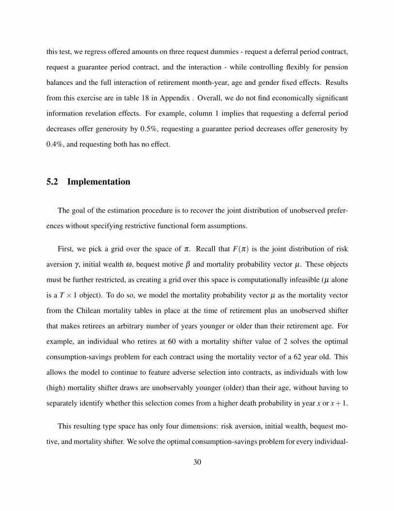
Panel A: CDF SummaryMass Cutoff 1.00E-01 1.00E-02 1.00E-03 1.00E-04
Number of Points with Mass Greater than Cutoff 1 26 48 50Total Mass for these Points 21.58% 89.26% 99.87% 100.00%
Panel B: Top 10 Mass PointsBequest Motive Risk Aversion Outside Wealth Health Shifter Mass 95% CI
1 621 0.000 10.100 15 21.58% (20.02%, 23.14%)2 7.89E+03 5.000 0.200 -1 7.57% (6.33%, 8.81%)3 0.414 0.000 0.200 15 6.16% (5.23%, 7.09%)4 137 1.875 0.200 -15 4.26% (3.10%, 5.42%)5 7.89E+03 4.375 0.200 -1 4.11% (2.82%, 5.40%)6 0.000289 0.625 16.288 15 3.86% (2.83%, 4.90%)7 44.6 0.625 18.762 -3 3.49% (2.07%, 4.92%)8 17.5 0.000 8.862 -1 2.66% (2.30%, 3.03%)9 3.59 0.000 11.338 -1 2.66% (2.30%, 3.03%)
10 44.6 1.875 0.200 -3 2.65% (1.14%, 4.16%)Notes: Panel A reports the number of points whose estimated mass is above different values and the totalmass for those points. Panel B reports the ten points with the highest estimated masses, as well as theirestimated weights and 95% confidence regions. These confidence intervals are calculated using clusteredstandard errors at the individual level.
Table 3: Descriptive Statistics for Estimated Type Distribution - Third Quartile Females
6.1 Estimates
As described in the previous section, we estimate the model separately for each combination
of gender and pension balance quartile. For clarity and brevity, we present results for women in
the third pension balance quartile here, and report results for all other female balance quartiles
in Appendix C. Results for males are available upon request. We focus on this subgroup as our
sample is predominantly female, and their relatively higher levels of pension savings (between
US$88,000 and US$135,000) make them more comparable to other settings. Table 3 presents the
10 grid points with highest estimated mass for this subsample, while figure 7 presents marginal
distributions for each dimension of unobserved type. We report standard errors that are clustered
at the individual level.31
The estimated type distribution is disperse, with only one point with mass greater than 10%, 26
31These standard errors are conservative, as they do not take into account that the true parameter cannot be negative- see Fox et al. (2011).
34
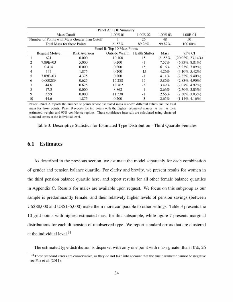
Figure 7: Marginal Distributions - Females in the Third Quartile of Pension Savings
points with mass greater than 1%, and 48 points with mass greater than 0.1%. Considering only
the 50 points with mass greater than 0.01% results in almost perfect coverage (99.9997%) of the
full type distribution. The distribution of the health age shifter32 exhibits substantial heterogeneity,
with 50.5% of retirees exhibiting higher death probabilities than those in the Chilean authorities’
table. In particular, there is large mass assigned to the health shifter value of 15. For a 60 year old
woman, a mortality shifter value of 15 corresponds to a life expectancy of approximately 75 years.
As for bequest motives, around 12% of retirees in this group behave as if they assign no value
to leaving money to their heirs, but there is also significant mass at the largest values of the grid.
This heterogeneity in bequest motive, and its correlation with mortality, plays an important role in
equilibrium outcomes and in counterfactuals, as individuals with high bequest motives value annu-
itization less, even if it comes at an actuarially fair price. In particular, a mandatory annuitization
32Recall that an individual who retires at age x with a health shifter of y solves the optimal consumption-savingsproblem with the mortality expectations of an x+ y year old according to the Chilean mortality tables.
35

policy is likely to significantly decrease the utility of this population as well as greatly reduce their
demand for annuities. We will return to this issue below.
The distribution of outside wealth has a large mass point at the lowest value in the grid (US$
8,170), consistent with survey evidence (Comision Asesora Presidencial Sobre el Sistema de Pen-
siones (2015)) that for many retirees pension savings are their lone asset for funding consumption
after retirement. Despite this, there is also substantial mass at the highest points in the grid. We
believe this is reasonable, considering that this object is meant to capture the value of all assets
that can fund consumption and inheritance, and that our sample is restricted to individuals who can
fund an annuity offer above the minimum pension.
Finally, the marginal distribution of risk aversion has large mass at γ = 0, which corresponds
to risk neutrality, and most mass below γ = 3. The mean of the distribution of γ is 1.39.
6.2 Correlations
In this setting, marginal distributions do not tell the whole story, as the relationship between the
unobservables will greatly affect choices and equilibrium outcomes. In particular, if individuals
with low mortality expectations also have high preferences for annuities due to other unobserved
characteristics, then the annuity market can feature advantageous, not adverse, selection. A nice
feature of our estimation procedure is that we are non-parametrically estimating the joint distribu-
tion of unobserved types, allowing us to flexibly determine the relationship between these unob-
servables. Table 4 presents these correlations for females in the third quartile of pension balances.
Other groups are reported in Appendix C.
The strongest correlations correspond to risk aversion and bequest motive (0.76), risk aversion
and outside wealth (-0.56), and risk aversion and the health shifter (-0.52). The first correlation
36

Bequest Motive Risk Aversion Outside Wealth Health ShifterBequest Motive 1.00 0.76 -0.34 -0.22Risk Aversion 0.76 1.00 -0.56 -0.52
Outside Wealth -0.34 -0.56 1.00 0.24Health Shifter -0.22 -0.52 0.24 1.00
Table 4: Correlations Across Dimensions of Unobserved Type - Third Quartile Females
is likely to be reflective of the choice of annuities with a guarantee period, as such a contract is
valuable to individuals who highly penalize both outliving their funds (or they would not annuitize)
and leaving no money to heirs (or they would not choose a guarantee period). The second correla-
tion is intuitive, as higher outside wealth means that individuals can self-insure. Finally, a negative
correlation between risk aversion and the health shifter implies that risk averse individuals have
longer life expectancies, perhaps due to a lower propensity to smoke and engage in risky behaviors,
and their higher consumption of preventative healthcare (Anderson and Mellor (2008))33. There is
also negative correlation between outside wealth and bequest motive, perhaps due to the fact that
richer retirees also have richer heirs, as one would expect in a country with low (albeit improving)
intergenerational mobility of income (Torche (2005), Sapelli (2016)).
Focusing on the health shifter, we find a negative correlation between this unobservable and
bequest motives, and a positive correlation with outside wealth. To illustrate the effects of these
correlations on annuity demand, we calculate the fraction of wealth each type would annuitize if
given a choice between an actuarially fair annuity and programmed withdrawal, and integrate out
over all dimensions of unobserved type except for mortality shifter. Figure 8 presents a scatter plot
of the value of the mortality shifter and the average fraction of wealth annuitized for that shifter
value. Naturally, higher values of the mortality shifter correspond to lower annuitization rates, as
these individuals are shorter lived. As a result, it is not surprising that the best fit line across these
33Our analysis abstracts away from moral hazard, meaning that we assume the choice to annuitize and to purchasea particular contract type does not determine life expectancy. We do not think that this assumption is restrictive, giventhat net NPVs for these contracts are not too dissimilar.
37
points is decreasing. However, the scatter plot shows substantial non-monotonicity in the rela-
tionship between health shifter and fraction annuitized. This highlights that the correlation across
dimensions of unobservables plays a significant role in determining equilibrium outcomes. In a
setting where mortality realizations are independent of all other dimensions of type, willingness
to pay for an annuity (conditional on gender, age and pension balances) solely depends on these
expectations.34 As a result, the first annuitized dollars in this market will correspond to individuals
who expect to be long lived. If these expectations are correct, this will induce adverse selection.
However, if other dimensions of unobserved type are correlated with mortality, this result can be
overturned. For example, our demand estimates imply that higher bequest motives are associated
with longer life expectancies. As a result, long lived individuals have less of an incentive to annu-
itize than predicted under the assumption of independence across types. This pushes the annuity
market towards advantageous selection. As a counterexample, a negative correlation between risk
aversion and health shifter - or positive correlation between risk aversion and life expectancy -
implies that the individuals who have the greater disutility of outliving their money are also the
most expensive to annuitize. We return to the issue of advantageous versus adverse selection into
annuitization below.
6.3 Model Fit and Equilibrium
Before discussing these issues, Table 5 presents various measures of in-sample and out-of-
sample fit of the demand estimation model, by gender-pension balance quartile. The model does
a reasonable job fitting the observed choices, despite ruling out any non-financial value of an an-
nuity offer. This is particularly true for the take-up of any annuity versus programmed withdrawal
(“Fraction Annuitized”), and for the fraction of individuals accepting an offer that mixes an annu-
ity with programmed withdrawal (“Fraction in Mixed Annuities”). However, it under-predicts the
34Which is the relevant conditioning set of variables in Chile, as all of these quantities are observed and priced on
38

Figure 8: Fraction of wealth annuitized, when choosing between PW and an actuarially fair annu-ity, as a function of the mortality shifter
fraction of individuals who take a deferred annuity and the fraction of individuals who take a guar-
anteed annuity. The bulk of this under-prediction stems from the fact that the model has difficulty
rationalizing acceptances of annuities with both a deferral period and a guarantee period. Deferral
periods are only valued by individuals who expect to be long-lived enough to recoup the “invest-
ment” of not receiving payoffs for a few years, while guarantee periods are only attractive to agents
with a significant bequest motive who have a non-trivial probability of death before the guarantee
period expires.35 This under-prediction is therefore to be expected from our model. Nevertheless,
we are reassured by the fact that the model fits the (out-of-sample) two-year mortality well, which
suggests that we are in fact recovering reasonable estimates of the distribution of unobserved types
from our model.
We now turn to the analysis of the annuity market equilibrium. Our goal is to analyze the im-
35We suspect that adding behavioral types, such as loss-averse retirees, could address this issue (Shu, Zeithammerand Payne (2016)).
39

Wealth Quartile First Second Third FourthFraction AnnuitizedObserved 66.89% 76.60% 75.30% 65.80%Predicted 58.77% 70.37% 71.53% 64.40%Fraction in Mixed AnnuitiesObserved 5.64% 7.93% 9.54% 6.26%Predicted 4.24% 5.16% 6.66% 5.14%Fraction in Deferred, Non-Guaranteed AnnuitiesObserved 3.07% 3.53% 3.77% 3.51%Predicted 4.52% 7.49% 8.07% 6.58%Fraction in Deferred & Guaranteed AnnuitiesObserved 17.16% 29.79% 33.05% 23.11%Predicted 4.76% 11.19% 14.16% 10.22%Fraction in Guaranteed, Non-Deferred AnnuitiesObserved 37.08% 35.12% 30.61% 29.79%Predicted 31.36% 34.49% 33.64% 32.10%Two-Year MortalityObserved 1.87% 1.71% 1.69% 1.94%Predicted 1.55% 1.71% 1.39% 1.23%Number of Offers 227332 366987 593671 428247Number of Individuals 8433 8409 10697 6585MSE 0.03 0.02 0.02 0.01R2 0.30 0.23 0.22 0.26
Table 5: Measures of In-Sample and Out-of-Sample Fit
40

Figure 9: Simulated Equilibrium under Baseline Policy - Third Quartile Females
plied annuity demand and average cost curves in the baseline Chilean setting, and to then study how
these functions are affected by changing the institutional setup. To do so, we analyze the equilib-
rium of a perfectly competitive annuity market where retirees can distribute their pension savings,
dollar for dollar, into either an immediate annuity with no guarantee period or programmed with-
drawal (with no minimum pension guarantee). Even in this basic setting, incorporating mandatory
annuitization and the ability to take lump-sum withdrawal can lead to market unravelling. Note
that since age, gender and pension balances can be priced on, every combination of these quan-
tities constitutes a separate market with potentially different equilibria. In what follows, every
equilibrium that is presented will be conditional on a combination of these quantities.
Figure 9 presents the implied annuity demand curve and average cost curve for a 60 year old
female retiree that retires with a pension balance equal to the third quartile of the distribution of
pension balances for females during our sample period.36 We construct the annuity demand curve
36Results for females in other quartiles are similar, and are presented in Appendix C.
41

by choosing a grid over the space of yearly annuity payouts (expressed as a percentage of the
pension balance) and, for every type and payout combination, solving for the optimal allocation
of pension balance between PW and an annuity. This gives us the fraction of wealth that each
type would annuitize across the grid of annuity payouts. We then aggregate to the market level
using the estimated type probabilities, and plot the curve relating annuity payouts to the aggregate
fraction of wealth annuitized - the demand curve in this setting. This curve can also be interpreted
as a “willingness-to-accept” curve, expressing the worst annuity offer that induces the marginal
annuitized dollar. We calculate the average cost curve by calculating the expected cost of a unit
annuity for every type, and then using the fraction of wealth each type annuitizes given a price and
the type probabilities to obtain the expected cost for the annuitant population at each price. We
express this expected cost in the same units as the demand curve, so that it can be interpreted as
the break-even annuity offer given the expected cost of the annuitant population. Under adverse
selection, this curve is upward-sloping: dollars that are only annuitized after high offers correspond
to individuals with higher mortality. Under advantageous selection, on the other hand, the curve is
downward sloping. Under our framework, the average cost curve can have regions of advantageous
selection and regions of negative selection, depending on the relative mortality expectations of the
marginal and inframarginal annuitants.
In figure 9, we find that the equilibrium for third quartile women features an equilibrium annu-
ity offer of 5.14% of the pension balance per year and 43.3% of total pension wealth annuitized.
The annuity demand curve is non-linear, reflecting the significant heterogeneity in the distribution
of types found earlier. Relatedly, the average cost curve is non-monotonic, with regions of adverse
and advantageous selection. In particular, we find a region of advantageous selection around the
market equilibrium, although globally the average cost curve exhibits adverse selection. Moreover,
the impact of adverse selection on the fraction of wealth annuitized is significant: the actuarially
fair payout for the whole population is 12% higher than the equilibrium payout, and at the actuari-
42

ally fair amount around 64% of available funds would be annuitized.
It is important to note that the preceding figures are not a good metric for quantifying the fit of
the model, as we have removed several features of the Chilean system in order for these equilibria
to be a reasonable benchmark for the counterfactuals that follow. In particular, we are removing the
possibility of bankruptcy, the minimum pension guarantee, programmed withdrawal commissions,
and multidimensional annuity contract types. These assumptions simplify the problem and allow
us to focus on the shifts in demand and average cost induced by changing the rules governing how
funds can be accessed.
6.4 Counterfactual Reforms
We now consider potential reforms to the current Chilean system. First, we remove the limi-
tations the government places on drawdown, and instead allow retirees to access their full pension
savings at retirement. The outside option to purchasing an annuity is free disposal of the entire
lump-sum.37 The unconstrained option keeps the benefits of PW, including the ability to pass
money to heirs and higher liquidity, and adds additional liquidity. That means every type would
prefer unconstrained lump-sum withdrawal to programmed withdrawal. Figure 10 shows the im-
pact of redesigning retirement policy in this way on the private annuity market equilibrium for the
same third quartile female as in the previous section. The remaining groups are in Appendix C.
This improvement in the outside option shows the same crowding out behavior demonstrated in
the calibration. Demand shifts downwards, and average cost changes shape with a local increase in
adverse selection near the reformed equilibrium. As a result, the new equilibrium annuity provides
a payout of 4.9% of pension wealth and the equilibrium level of annuitization drops to about
32%. Comparing the baseline and reformed equilibrium, we can see that the unconstrained lump
37This option is similar to what is available in Peru, where 95.5% of funds are available for lump-sum withdrawal.
43
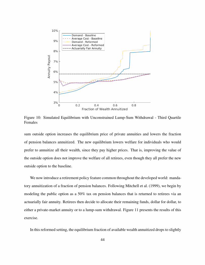
Figure 10: Simulated Equilibrium with Unconstrained Lump-Sum Withdrawal - Third QuartileFemales
sum outside option increases the equilibrium price of private annuities and lowers the fraction
of pension balances annuitized. The new equilibrium lowers welfare for individuals who would
prefer to annuitize all their wealth, since they pay higher prices. That is, improving the value of
the outside option does not improve the welfare of all retirees, even though they all prefer the new
outside option to the baseline.
We now introduce a retirement policy feature common throughout the developed world: manda-
tory annuitization of a fraction of pension balances. Following Mitchell et al. (1999), we begin by
modeling the public option as a 50% tax on pension balances that is returned to retirees via an
actuarially fair annuity. Retirees then decide to allocate their remaining funds, dollar for dollar, to
either a private-market annuity or to a lump-sum withdrawal. Figure 11 presents the results of this
exercise.
In this reformed setting, the equilibrium fraction of available wealth annuitized drops to slightly
44
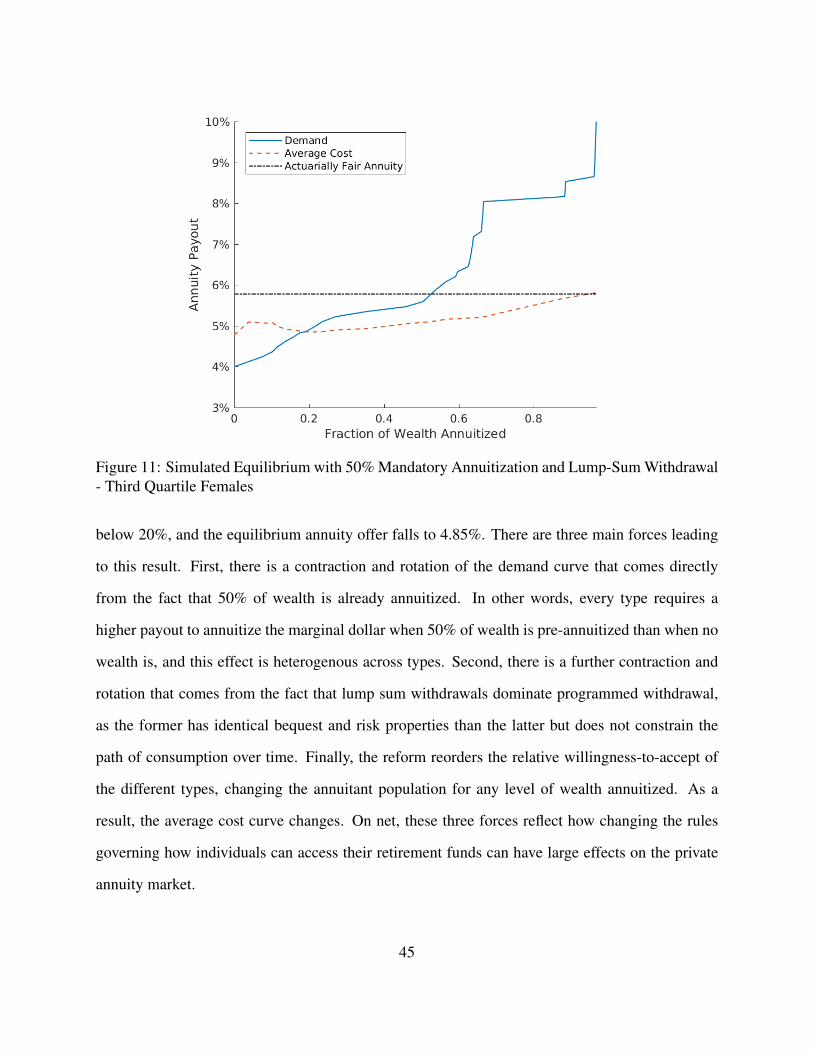
Figure 11: Simulated Equilibrium with 50% Mandatory Annuitization and Lump-Sum Withdrawal- Third Quartile Females
below 20%, and the equilibrium annuity offer falls to 4.85%. There are three main forces leading
to this result. First, there is a contraction and rotation of the demand curve that comes directly
from the fact that 50% of wealth is already annuitized. In other words, every type requires a
higher payout to annuitize the marginal dollar when 50% of wealth is pre-annuitized than when no
wealth is, and this effect is heterogenous across types. Second, there is a further contraction and
rotation that comes from the fact that lump sum withdrawals dominate programmed withdrawal,
as the former has identical bequest and risk properties than the latter but does not constrain the
path of consumption over time. Finally, the reform reorders the relative willingness-to-accept of
the different types, changing the annuitant population for any level of wealth annuitized. As a
result, the average cost curve changes. On net, these three forces reflect how changing the rules
governing how individuals can access their retirement funds can have large effects on the private
annuity market.
45

Figure 12: Equilibrium Fractions of Wealth Annuitized and Annuity Payouts as a Function of theFraction of Wealth in the Mandatory Annuity - Third Quartile Females
We expand the set of counterfactual reforms to include other levels of mandatory annuitization,
ranging from 0% to 90%. That is, we find the equilibrium level of private annuitization, given
that retirement policy prescribes that retirees have x% of their wealth annuitized at the actuarially
fair price, and the remaining 1-x% is free to be allocated between an annuity and a lump sum
withdrawal. Figure 12 plots the equilibrium fraction of wealth annuitized (left axis) and the equi-
librium annuity payout relative to the actuarially fair annuity (right axis) as a function of mandatory
annuitized wealth fraction.
The solid line shows that increasing the fraction of mandatory annuitization monotonically
crowds out private annuity transaction volumes. Annuitized wealth starts at 32% in the uncon-
strained lump sum case (labeled ”0%”) and continues to drop, with only 10% of remaining wealth
being annuitized privately when 90% of pension wealth is required to be annuitized. The equilib-
rium annuity price changes nonmonotonically as policies change. Annuity generosity decreases
46

as the fraction of wealth in a mandatory annuity rises from 0% to 50%. This is consistent with
adverse selection, meaning that retirees who already have 50% of their wealth in an actuarially fair
annuity have a lower willingness to pay for additional annuitization than those who have no money
in an annuity. Interestingly, annuity payouts improve when moving from 50% to 75% mandatory
annuitization, and improve further when moving to 90%. Demand is still contracting in each of
these shifts, as reflected by the falling annuitization rate, so it must be the case that the increase in
payouts is coming from a more advantageously selected annuitant population. That is, the effect of
additional amounts in the mandatory annuity on equilibrium prices are moderated by advantageous
selection.
6.5 Welfare
The welfare effect of reforming the system is theoretically uncertain. Individuals with strong
preferences for full annuitization in all cases have higher welfare with higher mandatory annuiti-
zation, since those annuities are actuarially fair. Other individuals’ welfare depends on the tradeoff
between more unconstrained wealth due to the elimination of PW and forced annuitization that may
be unwanted. To sign these overall effects and to measure the distribution of gains and losses, we
quantify the welfare comparison between the baseline Chilean system and its reformed versions.
To do so, we calculate for each type their equivalent variation, or the transfer into their base-
line pension balance that would make them indifferent between retiring under the baseline or the
reformed rules. More precisely, define V ∗B (W0,θr) to be type θr’s utility derived from their optimal
allocation of pension balance W0 across programmed withdrawal and an annuity at the baseline
equilibrium price, and define V ∗Rx%(x% ·W0,(1− x%) ·W0,θr) to be type θr’s utility derived from
their optimal allocation of remaining pension balance (1− x%) ·W0 across lump sum withdrawal
and an annuity at the equilibrium price when x% of funds are placed in a mandatory annuity. This
47
latter utility, of course, takes into account that x% ·W0 is returned to retirees through an actuari-
ally fair annuity. Then the equivalent variation for type θr between the baseline and the reformed
system with x% allocation to the mandatory annuity solves
V ∗B (W0 +EV (x%,θr),θr) =V ∗Rx%(x% ·W0,(1− x%) ·W0,θr)
We plot the resulting distribution of equivalent variation for the unconstrained lump sum and
the 50% mandatory annuitization reforms in Figure 13. The plot shows that moving to an uncon-
strained lump sum outside option, which increases the value of the outside option to all retirees,
would causes a welfare loss equivalent to $5,000 or less for 45% of our sample. Another 45% see
modest welfare gains from the reform. Finally, about 10% of our retirees see large welfare benefits
from releasing constraints on drawdown. These retirees are high mortality, low outside wealth,
and zero bequest motive types. They choose PW in the baseline as it is front-loaded relative to the
annuity, but would prefer an option that allows them to consume more and leave less money upon
their death. On average, the reform improves welfare, but those gains are driven by a small fraction
of the population. The effect of introducing 50% mandatory annuitization as the outside option has
a different effect. This reform causes lost utility for the just 25% of our sample, though they face a
larger magnitude of loss up to $18,000 in wealth equivalent. The remaining 75% benefit from the
reform, in wealth equivalents between $3,000 and $30,000. Mandatory annuitization has a more
evenly distributed effect compared to the unconstrained lump sum case.
Then, we compare the distribution of welfare benefits and costs across different levels of
mandatory annuitization. The left panel of figure 14 plots the cumulative distribution functions
of equivalent variation for third quartile females across different values of the fraction of wealth in
the mandatory annuity, while the right panel plots the average and median EV for each counterfac-
tual equilibrium.
48

Figure 13: CDF of equivalent variation, for third quartile females, for unconstrained lump sum and50% mandatory annuity reform.
Figure 14: CDF of equivalent variation (left) and mean equivalent variation (right), for third quar-tile females, across different amounts in the mandatory annuity.
49

Focusing on the right panel, the average equivalent variation is positive for all values of wealth
in the mandatory annuity, suggesting that on average retirees would prefer any version of the re-
formed system to the baseline Chilean case. Moreover, the 0% mandatory annuitization case,
where the outside option is changed to lump-sum withdrawal but the system is otherwise un-
changed, yields the highest average equivalent variation: on average, retirees would value it equiv-
alently to an increase in their pension balance of 5,000 dollars in the baseline. As the fraction
of wealth in the mandatory annuity increases, the average equivalent variation monotonically de-
creases.
However, the CDFs presented on the left panel of figure 14 highlight that this average equiv-
alent variation masks significant heterogeneity across the population. In fact, no version of the
reformed system Pareto dominates the baseline equilibrium, as there is significant mass in both the
space where retirees prefer the baseline to the reformed (negative values of EV) and in the space
where the converse holds. For example, the distribution of EV when 50% of wealth in placed
in the mandatory annuity exhibits retirees who are are indifferent between this reformed system
and being given around $30,000 dollars in the baseline and individuals for whom the transfer that
would make them indifferent is around -$16,000. Returning to the right panel, the very different
pattern exhibited by the median of the EV distribution highlights this heterogeneity. Median wel-
fare is lowest when mandatory annuitization is set at 0% or 25%. Median welfare grows through
50% mandatory annuitization, and peaks at 75% mandatory annuitization. Depending on the social
welfare function, different levels of mandatory annuitization maximize overall retiree welfare.
6.6 Discussion
The previous results show that reforming the system to incorporate mandatory annuitization
of a fraction of wealth, combined with a relaxation of the drawdown path for the alternative to
50

annuitization, has the potential to increase welfare for the average retiree, although no reform is
Pareto improving. There are three natural concerns with these results.
First, we have not modelled the contribution phase of this retirement system, and any reforms
will have implications on savings during the working life. This argument does not invalidate this
exercise if the objective is to study what soon-to-be retirees would choose in a counterfactual
system, as they do not have the ability to greatly change their pension savings or their outside
wealth in response to the reform. However, it does cast doubt on the ability to make statements
about welfare for individuals who have the time to respond to the reform by significantly changing
their savings. We believe that this is an interesting question for future research.
Second, we have not introduced behavioral biases into the model, and as a result cannot speak
to time inconsistencies that can arise from having a large sum of money immediately available. To
that end, perhaps the introduction of both lump sum withdrawal and mandatory annuitization of a
small fraction of pension balances is more desirable than a system with no mandatory annuitization,
even though the latter delivers a higher average welfare change.
Finally, one can argue that the natural welfare metric here should be Rawlsian, as the objective
of pension systems is to insure a consumption floor for all individuals in the population. Therefore,
one should assess the previous findings through the lens of their effects on the welfare of the
poorest individuals in the population, and not on the average. To explore this issue, figure 15
presents the same distributions of equivalent variation as before, but now conditioning on the types
with the lowest levels of inside and outside wealth - the poorest individuals in our sample. For this
subpopulation, we find that reforming the system to include lump sum withdrawal and mandatory
annuitization of a fraction of wealth between 25% and 75% yields a Pareto improvement relative
to the baseline.
51

Figure 15: CDF of equivalent variation for first quartile female types with the lowest levels ofoutside wealth, across different amounts in the mandatory annuity.
7 Conclusion
The Chilean annuity market has several striking features. First, a large majority of retirees
choose to purchase private annuities with their retirement savings. Second, prices of annuities in
equilibrium are 3-5% more expensive than actuarially fair, significantly cheaper than the 10-15%
markup over actuarial fairness estimated in the US. Third, the Chilean market exhibits evidence of
adverse selection, as do many other annuity markets.
The evidence laid out in the reduced form facts and calibrations imply that, under certain pa-
rameters, Chile’s annuity market may be crowded in by the absence of a public mandatory pension
system. That is, the market could unravel if retirement policy was reformed to remove retirees’
choice between constrained withdrawal and private annuitization, and replace it with a mandatory
system. Furthermore, the shape of the demand and average cost curves found in the calibration
52
exercise make it clear that simple reduced form estimation approaches are not well suited to de-
termine whether the market will unravel under counterfactual regulatory regimes or to study the
welfare implications of these reforms. To overcome these challenges, we build a structural model
based on the standard consumption-savings problem faced by retirees, that accounts for income ef-
fects and other features of nonlinear utility that influence retirees’ choices. The aim is to estimate
the distribution of unobservable retiree characteristics from which we can derive their demand for
annuities and the cost firms face to insure them. The model adapts the methodology developed
by Fox et al. (2011). We pre-solve this lifecycle model for a representative set of consumers over
a wide variety of combinations of unobserved preferences. We then estimate the distribution of
weights on the distribution of consumers that allows us to match moments observed in the data.
Demand estimates show that individuals have significant and highly varied private information
about their own mortality, bequest motives, risk aversion, and outside wealth. Armed with these
demand estimates, we simulate market equilibria under existing Chilean policies, as well as under
counterfactual retirement policy which removes limits on drawdown of retirement savings and in-
troduces a mandatory pension for all retirees. Though the private annuity market partially unravels
if retirement policy is reformed, retiree welfare increases on average. However, this masks signif-
icant heterogeneity in the impact of these reforms. Even replacing the constrained “programmed
withdrawal” of retirement assets with an unconstrained lump sum, which is a better product for all
retirees, causes welfare loss to annuitants who now face higher prices in the crowded out private
market. Overall, our results highlight the importance of assessing policy reforms by quantifying
both their direct effect on individuals and their indirect crowd-out or crowd-in of private market
equilibria. These effects are particularly complicated in markets with multiple dimensions of pri-
vate information. Our method of nonparametrically estimating demand provides one way forward
for evaluating such policies in other contexts, since it allows for any shape of demand and average
cost and it allows for the valuation of out of sample products. By solving for the full distribution
53

of welfare gains and losses, our method provides the building blocks for policymakers looking to
estimate the impact of large scale policy reforms on individuals with highly heterogeneous prefer-
ences.
References
Alcalde, Pilar, and Bernardita Vial. 2017. “Implicit Trade-off in Replacement Rates: Consumer
Preferences for Firms, Intermediaries, and Annuity Attributes.”
Anderson, Lisa R., and Jennifer M. Mellor. 2008. “Predicting Health Behaviors With an Exper-
imental Measure of Risk Preference.” Journal of Health Economics, 27(7): 1260–1274.
Bernartzi, Shlomo, Previtero Alessandro, and Richard H. Thaler. 2011. “Annuitization Puz-
zles.” Journal of Economic Perspectives, 25(4): 143–164.
Brown, Jeffrey R., and Amy Finkelstein. 2008. “The Interaction of Public and Private In-
surance: Medicaid and the Long-Term Care Insurance Market.” American Economic Review,
98(3): 1083–1102.
Brown, Jeffrey R., Arie Kapteyn, Erzo F. P. Luttmer, and Olivia S. Mitchell. 2017. “Cognitive
Constraints on Valuing Annuities.” Journal of the European Economic Association, 15(2): 429–
462.
Brown, Jeffrey R., Norma B. Coe, and Amy Finkelstein. 2007. “Medicaid Crowd-Out of Private
Long-Term Care Insurance Demand: Evidence from the Health and Retirement Survey.” Tax
Policy and the Economy, 21: 1–34.
Bundorf, M. Kate, and Kosali I Simon. 2006. “The Effects of Rate Regulation on Demand for
Supplemental Health Insurance.” American Economic Review, 96(2): 67–71.
54

Butler, Monika, and Federica Teppa. 2007. “The Choice Between an Annuity and a Lump Sum:
Results from Swiss Pension Funds.” Journal of Public Economics, 91: 1944–1966.
Caliendo, Frank N., Nick L. Guo, and Roozbeh Hosseini. 2014. “Social security is NOT a
substitute for annuity markets.” Review of Economic Dynamics, 17(4): 739–755.
Carroll, Christopher D. 2006. “The method of endogenous gridpoints for solving dynamic
stochastic optimization problems.” Economics Letters, 91(3): 312 – 320.
Carroll, Christopher D. 2011. “Solution Methods for Microeconomic Dynamic Stochastic Opti-
mization Problems.”
Castro, Sebastian, Felipe Castro, Jacinta Diestre, and Luis Munoz. 2018. “Estudio de Mercado
sobre Rentas Vitalicias.” Division Estudios de Mercado, Fiscalıa Nacional Economica.
Chiappori, PierreAndre, and Bernard Salanie. 2000. “Testing for Asymmetric Information in
Insurance Markets.” Journal of Political Economy, 108(1): 56–78.
Comision Asesora Presidencial Sobre el Sistema de Pensiones. 2015. “Informe Final Comision
Asesora Presidencial Sobre el SIstema de Pensiones.” Ministerio del Trabajo y Prevision Social.
Compendio de Normas del Sistema de Pensiones, Capıtulo III: Factor Actuarialmente Justo.
2018.
Crivelli, Luca, Massimo Filippini, and Ilaria Mosca. 2006. “Federalism and regional health care
expenditures: an empirical analysis for the Swiss cantons.” Health Economics, 15(5): 535–541.
Cullen, Julie Berry, and Jonathan Gruber. 2000. “Does Unemployment Insurance Crowd out
Spousal Labor Supply?” Journal of Labor Economics, 18(3): 546–572.
Cutler, David, and Jonathan Gruber. 1996. “Does Public Insurance Crowd out Private Insur-
ance?”
55

Davidoff, Thomas, Jeffrey R. Brown, and Peter A. Diamond. 2005. “Annuities and Individual
Welfare.” American Economic Review, 95(5): 1573–1590.
Einav, Liran, Amy Finkelstein, and Paul Schrimpf. 2010. “Optimal Mandates and the Welfare
Cost of Asymmetric Information: Evidence From the U.K. Annuity Market.” Econometrica,
78(3): 1031–1092.
Einav, Liran, Amy Finkelstein, and Pietro Tebaldi. 2019. “Market Design in Regulated Health
Insurance Markets: Risk Adjustment vs. Subsidies.” Mimeo.
Finkelstein, Amy, and Kathleen McGarry. 2006. “Multiple Dimensions of Private Informa-
tion: Evidence from the Long-Term Care Insurance Market.” American Economic Review,
96(4): 938–958.
Finkelstein, Amy, Nathaniel Hendren, and Mark Shepard. 2017. “Subsidizing Health Insur-
ance for Low-Income Adults: Evidence from Massachusetts.” National Bureau of Economic
Research Working Paper 23668.
Fox, Jeremy T., Kyoo il Kim, and Chenyu Yang. 2016. “A simple nonparametric approach to es-
timating the distribution of random coefficients in structural models.” Journal of Econometrics,
195(2): 236 – 254.
Fox, Jeremy T., Kyoo il Kim, Stephen P. Ryan, and Patrick Bajari. 2011. “A simple estimator
for the distribution of random coefficients.” Quantitative Economics, 2(3): 381–418.
Friedman, Benjamin M., and Mark J. Warshawsky. 1990. “The Cost of Annuities: Implications
for Saving Behavior and Bequests.” The Quarterly Journal of Economics, 105(1): 135–154.
Garthwaite, Craig, Tal Gross, and Matthew J. Notowidigdo. 2018. “Hospitals as Insurers of
Last Resort.” American Economic Journal: Applied Economics, 10(1): 1–39.
56

Gruber, Jonathan, and Kosali I Simon. 2008. “Crowd-out 10 years later: Have recent public
insurance expansions crowded out private health insurance?”
Hackmann, Martin B., Jonathan T. Kolstad, and Amanda E. Kowalski. 2015. “Adverse Se-
lection and an Individual Mandate: When Theory Meets Practice.” American Economic Review,
105(3): 1030–1066.
Hosseini, Roozbeh. 2015. “Adverse Selection in the Annuity Market and the Role for Social Se-
curity.” Journal of Political Economy, 123(4): 941–984.
Illanes, Gaston. 2019. “Switching Costs in Pension Plan Choice.” Northwestern University
Mimeo.
Keane, Michael, and Olena Stavrunova. 2016. “Adverse selection, moral hazard and the demand
for Medigap insurance.” Journal of Econometrics, 190(1): 62–78.
Koch, Thomas G. 2014. “Bankruptcy, Medical Insurance, and a Law with Unintended Conse-
quences.” Health Economics, 23(11): 1326–1339.
Lockwood, Lee. 2012. “Bequest Motives and the Annuity Puzzle.” Review of Economic Dynamics,
15(2): 226–243.
Mahoney, Neale. 2015. “Bankruptcy as Implicit Health Insurance.” American Economic Review,
105(2): 710–746.
Mitchell, Olivia S., James M. Poterba, Mark J. Warshawsky, and Jeffrey R. Brown. 1999.
“New Evidence on the Money’s Worth of Individual Annuities.” American Economic Review,
89(5): 1299–1318.
Pino, Francisco. 2005. “Retiros Programados y Nuevas Tablas de Mortalidad.” Superintendencia
de Pensiones Nota Tecnica 1.
57
Reichling, Felix, and Kent Smetters. 2015. “Optimal Annuitization with Stochastic Mortality
and Correlated Medical Costs.” American Economic Review, 105(11): 3273–3320.
Rothschild, Casey G. 2009. “Adverse Selection in Annuity Markets: Evidence from the British
Life Annuity Act of 1808.” Journal of Public Economics, 93(10): 776–784.
Sapelli, Claudio. 2016. Chile ¿mas equitativo?: Una mirada a la dinamica social del Chile de
ayer, hoy y manana. . 2 ed., Ediciones UC.
Shiller, Robert J. 1998. “Indexed Units of Account: Theory and Assessment of Historical Expe-
rience.” National Bureau of Economic Research Working Paper 6356.
Shu, Suzanne B., Robert Zeithammer, and John W. Payne. 2016. “Consumer Preferences for
Annuity Attributes: Beyond Net Present Value.” Journal of Marketing Research, , (53): 240–
262.
Sloan, Frank A., and Edward C. Norton. 1997. “Adverse Selection, Bequests, Crowding Out,
and Private Demand for Insurance: Evidence from the Long-term Care Insurance Market.” Jour-
nal of Risk and Uncertainty, 15(3): 201–219.
Starc, Amanda. 2014. “Insurer pricing and consumer welfare: evidence from Medigap.” The
RAND Journal of Economics, 45(1): 198–220.
Tebaldi, Pietro. 2019. “Estimating Equilibrium in Health Insurance Exchanges: Price Competition
and Subsidy Design under the ACA.” Mimeo.
Torche, Florencia. 2005. “Unequal but Fluid: Social Mobility in Chile in Comparative Perspec-
tive.” American Sociological Review, 70(3): 422–450.
Vega, George. 2014. “Capital Necesario Unitario (CNU): Calculo e Introduccion delModulo de
Stata cnu.” Superintendencia de Pensiones Nota Tecnica.
58