NBER WORKING PAPER SERIES

THE DYNAMIC DEMANDFOR CAPITAL AND LABOR

Matthew D. Shap-iro

Work-ing Paper No. 1899

NATIONAL BUREAU OF ECONOMIC RESEARCH1050 Massachusetts Avenue

Cambridge, MA 02138April 1986

The research reported here s part of the NBER1S research program-in Economic Fluctuations. Any op-inions expressed are those of theauthor and not those of the Nat-ional Bureau of Economic Research.

NBER Working Paper #1899April 1986

The Dynamic Demand for Capital and Labor

ABSTRACT

A model of the dynamically interrelated demand for capital and labor

is specified and estimated. The estimates are of the first—order conditions

of the firm's problem rather than of the closed—form decision rules. This

use of the first—order conditions allows a random rate of return and a

flexible specification of the technology. The estimates do not imply the

very slow rates of adjustment displayed in other, related estimates of the

demand for capital. Because adjustment is estimated to be rapid, there is,

contrary to the standard view, scope for factor—prices to affect investment

at relatively high frequencies.

Matthew D. ShapiroCowles Foundation for Research

in EconomicsYale University2125 Yale StationNew Haven, CT 06520(203) 436—0605

I. Introduction

There is a significant gap between the theory and empirical work in

the standard models of investment. This paper offers some plausible esti-

mates of investment dynamics that are both consistent with a structural

model and useful for policy analysis. Because the choice of capital stock

is inherently connected with the choice of other factors, labor in partic-

ular, the model is of capacity choice in general instead of investment in

particular. When a firm purchases or hires factors of production, it de-

termines its productive capacity. Short-run variation in output comes

principally from variation in factors that are adjustable at little or

no cost. Investment responds relatively slowly to shocks because of ad-

justment costs.

In this paper I provide structural estimates of demand for factors--

capital in particular. These estimates can be used for analyses of tax policy

that are immune from the Lucas critique. The dynamic response of invest-

ment implied by the estimates is more plausible than that found in previous

research. I use a model where the firm maximizes the present discounted

value of profits subject to a technology with adjustment costs. Such a

specification has a long history in the investment literature. Moreover,

it is a generalization of Tobin's q-model, which is equivalent to an ad-

justment cost model where only capital is costly to adjust. The firm chooses

its capital stock, its number of production and non-production workers,

and hours of production workers.

I estimate the first-order conditions, or Euler equations, of the

problem rather than the closed-form decision rules. The estimation tech-

nique is Hansen's [1982] generalized method of moments. To evaluate the

performance of the model, I consider its dynamic properties. My estimates

1

2

of the dynamic response of the capital stock do not have the implausibly

long adjustment lags found in other research. Because adjustment is rapid,

changes in interest rates and factor prices can affect the demand for capi-

tal at business cycle frequencies.

Factor prices determine investment in the neo-classical models of

Jorgenson and Hall (see Jorgenson [1963] and Hall and Jorgenson [1967]),

the cost-of-adjustment models (see Lucas [1967], Treadway [1969], and Lucas

and Prescott [1971]), and the q-models (see Brainard and Tobin [1968] and

Tobin [1969]). Abel [1979, 1982, 1983] and Hayashi [1982] show that the

cost-of-adjustment models and the q-models are essentially equivalent. I

use a generalization of the cost-of-adjustment model that takes into account

the choice of number of employees and their hours of work as well as the

choice of the stock of capital.

The q-approach has not yielded satisfactory estimates of the parameters

of the investment function. Abel and Blanchard [l983bJ resort to a sales-

investment specification because of their difficulty in usefully explaining

investment with q (see Abel and Blanchard [l983a] for the estimates with

q ). Their dissatisfaction with the q-approach does not arise from an

a priori defect in the theory but in its empirical performance. Although

the market value of publicly traded corporate capital is easy to measure,

it is difficult to measure its replacement cost. Moreover, the appropriate

concept in a q-equation is marginal rather than average q . Marginal

q cannot be directly measured, although it can in principal be constructed.

Indeed, a q is implied in the calculations in this paper. Nonetheless,

the implementation of the model in this paper does not depend on construct-

ing a series for q

Summers's 11981] paper highlights the problem with the estimates based

3

on q-theory. In particular, he finds extremely slow adjustment of the

capital stock to changes in factor prices. The estimates offered in this

paper do not have this shortcoming. By examining the adjustment problem

directly, rather than through a summary statistic such as q , I obtain

reasonable rates of adjustment.

II. The Firm's Decision Problem

The representative firm maximizes the present discounted value of

cash flow. The choice variables of the firm are the purchases of capital,

the net hires of employees, and the number of hours that the employees

work. I distinguish between production and non-production workers. These

choices determine output; thus, output is endogenous. The firm takes factor

prices and the investors' ex ante required rate of return as exogenous.

Stocks of factors are costly to adjust, so lagged factor stocks enter

the decision rule of the firm. That is, the firm in the short run does

not hire the long-run, profit-maximizing level of inputs. Because the

exogenous variables change over time, the firm takes into account their

expected path in making its current decisions. Since the time path of

factors determines the time path of output, no separate choice of capacity

utilization is made.

I now consider the individual components of real cash-flow: real

output, real labor cost, and real capital cost. I combine these below to

obtain the expression for discounted cash-flow.

4

A. Production Function

The real output of the firm is given by the production function

(1) = f(K, Lt, N, H, Kt_dKtl, L_q1L1

N_q1N1, Ht_Htl, X) = f(Z, LZt, X)

where is the stock of capital, Lt the number of production workers,

Nt the number of non-production workers, and Ht the average hours of

production workers. The parameter d is one minus the rate of depreciation

of capital and is one minus the quit rate, that is, the rate at which

the stock of workers depreciates. For notational convenience, Z and

denote, respectively, vectors of the levels and gross changes of the factors.

The vector X represents unobserved factors in the production function.

Trend productivity and shocks to the production function are the obvious

examples of such unobservables. Measured output, y , is value-added so

intermediate inputs are neglected.2

Output depends on the level and gross rate of change of the factors of

production. Output is allowed to depend on the rates of change of the inputs

to allow for adjustment costs. Brechling and Mortenson [1969] and Brechling

[1975] characterize in detail the properties of a production function such

as (1). The adjustment costs are internal to the production process. That

is, the cost of output lost when the factors of production are varied. This

cost does not represent specific payment to a factor. External adjustment

costs (such as the purchase cost of capital) are accounted for elsewhere.

In adjusting the stock of labor, output is lost through the inexper-

ience of new workers and the time taken to readjust the schedule and pattern

of production. Adjustment costs for the number of employees are likely

to be much more important than that for the average hours worked. Output

5

is lost when capital is adjusted through the lost production time during

installation, the difficulty of incorporating new machines into the pro-

duction process, and the labor input diverted to install the new capital.

The production function must be parameterized in order to render the

theory empirically useful. Some researchers estimate closed-form decision

rules rather than Euler equations. Examples are Sargent [1978], Kennan

11979], Meese 11980], and Hansen and Sargent [1980, 1982]. They specify

the production functions so the problems are linear quadratic. This spec-

ification yields closed-form decision rules under rational expectations.

Epstein and Denny [1983] offer a general functional form and then

approximate it for estimation. They assume static expectations, which is

a serious shortcoming given the explicitly dynamic nature of the problem.

Indeed, they do not specify the source of the randomness in the firm's

environment. As I discuss in Section IV, the structure of the error term

in the factor demand equations determines what instruments are valid to

identify the parameters. Therefore, it is difficult to evaluate the iden-

tification of their parameters in the absence of explicit assumptions about

the stochastic environment facing the firm. Epstein and Denny do discuss

the restrictions on the shape of the production function. In particular,

they test whether it is concave. An exception to the practice of using

quadratic approximations is Pindyck and Rotemberg [1983], who derive con-

ditional factor demands on the basis of trans-log cost functions.

I estimate the Euler equations themselves, rather than an approxi-

mated decision rule, that is, the solution of the Euler equation. This

procedure allows important complications to be introduced. These include

non-quadratic specifications of the production function, a non-linear

wage bill, and a variable rate of discount. Only efficiency of estima-

6

tion is lost by estimating the Euler equation instead of the decision

rules. In particular, the technique of Flansen and Sargent [1980, 1982]

of estimating the decision rules exploits the restrictions between the

demand equations and the stochastic processes of the variables on the other

side of the market. The decision rules also impose the transversality

conditions. The Euler equation and decision rules estimate the same param—

eters. More information (cross equation restrictions and transversality

conditions) are used to estimate the decision rules. This gain in efficiency

seems a high price to pay for restricting the rate of return to be constant

and for having to make strict assumptions about the technology. In this

research I need not impose the extreme restrictions on the structure of the

problem which are made by Hansen and Sargent to yield closed-form, rational

expectations solutions.

In presenting the basic results, I choose the Cobb-Douglas production

function for tractability and ease of interpretations. I also present

alternative estimates with a constant elasticity of substitution production

function. The Cobb-Douglass function has the advantage of simplicity so

one can inspect the parameters for the plausibility of their magnitudes

as well as for statistical significance. The results of other studies which

report production function parameters in terms of the steady-state values

of derivatives (that is, the quadratic specification commonly used in the

rational expectations literature), are difficult to evaluate. In particular,

assumptions of convexity and constant returns to scale are often neither

imposed nor tested.3

Many authors assume that employees and hours enter multiplicatively

in the production function. Both Sargent [1978] and Meese [1980] make

this assumption. Indeed, Meese makes the much stronger assumption that

7

firms choose man-hours alone instead of separately choosing number of em-

ployees and hours of work. (Sargent handles this issue by distinguishing

between straight-time and overtime hours.) Employees and hours have dif-

ferent marginal costs. Adding an hour may entail an overtime premium;

adding an employee may involve fixed costs such as health insurance. Em-

ployees and hours also have different adjustment costs. Hence, assuming

that the decision variable is man-hours rather than hours and employees

separately distorts the firm's choice problem even if hours and employees

enter the production function multiplicatively. Treating the decision

variable as man-hours instead of employees and hours separately may also

lead to an incorrect linearization of the production function even if

those variables enter it multiplicatively. Additionally,straight-time

and average overall wages vary insubstantially over the business cycle.

Overtime hours do vary substantially causing the marginal cost of an hour

worked to be higher than the basic data suggest. The dynamic factor demand

models rely on variation in factor prices to explain the dynamics of de-

mand; neglecting this substantial variation in cost is a mistake.

Some authors, such as Fair [1969], Nadiri and Rosen [1969], and Bernanke

[1983], stress that hours and employment may not enter multiplicatively

in the production function. In this paper, I also let them enter separately.

The production function I use for the basic results is

(2) log = log[f(Z, LZt, Xt)]= log Za - + X

where

8

a = (aK, aL, aN, aH)

symmetric,

log Kt

log LtloZ = , and

logN.

log H

Kt - dKti

=L -

N -

Ht_Htl

That is, the log of output is a linear function of the log of the levels

of inputs minus a quadratic function of the gross changes of the inputs.

Hence, the production function is Cobb-Douglas augmented by adjustment

cost terms. The vector X denotes the productivity shock. It, in gen-

eral, will contain constant and trend terms as well as stochastic produc-

tivity shocks of arbitrary serial correlation. As long as enters

the production function additively in logs, it will drop out of the esti-

mated Euler equation. Hence, the productivity shock term need not be

parameterized.

I impose the constant-returns-to-scale restriction on output gross

of adjustment costs so that aK + aL+

aN= 1 The form of the function

9

implies convexity. There is no natural CRS restriction on the cost of

adjustment parameters. That part of the function is convex as long as

the matrix of the g parameters is positive definite. I do impose the

requirement that the matrix of the g parameters is symmetric. It is

useful to note that I do not restrict the coefficient of hours,Ht

when I impose constant returns to scale. It is natural to leave aH un-

restricted: a replication of capital and labor would presumably leave

hours per worker constant. The difference aH - aL measures the depar-

ture of employees and hours from entering the production function multi-

plicatively.

I assume that capital and labor have adjustment costs related to the

change in the stock. The adjustment cost for capital is a function of

the square of gross investment, Kt - dKtl . The depreciation rate is

taken to be parametric so the capital series can be derived from the gross

investment series. An alternative specification would be to use net invest-

ment. The rationale for using net investment would be that replacement

investment is somehow more routine and therefore less costly than net in-

vestment. Machines are rarely replaced one-for-one; consequently, there

is not a clear distinction between replacement and new investment. There-

fore, there is not a strong case of using net investment.

Likewise, the adjustment cost for employees is proportional to the

gross change in the number of employees, Lt - q1L1 and Nt - q_1_1where is one minus the quit rate. As with the depreciation rate,

the firm takes the quit rate as given. Unlike the depreciation rate, the

quit rate is published data and varies across time. The choice variable

of the firm is the current stock of employees. In arriving at the figure

it takes into account the probability that a fraction of the workers will

10

quit each period.

I also allow there to be interrelated adjustment costs in (2). These

arise if the lost production time through adjusting one factor is greater

or less when the firm adjusts other factors.

I expect there to be little or no cost to adjusting hours. Firms

can adjust hours merely by extending the length of the shift. (Diminish-

ing marginal product is, of course, captured in the production function.)

Such an adjustment is likely to be much easier than adding a worker. In

particular, extending the operation of the plant for an hour requires no

realignment of workers and machines. An extra worker, on the other hand,

must be incorporated into the pattern of production.

B. Cost of Labor

Now I consider the cost of the labor to the firm. Labor cost is a

function of the number of employees, the hours they work, and rate of com-

pensation of employees not sensitive to hours worked. Compensation not

sensitive to hours worked includes all payments to salaried employees and

certain non-wage payments to hourly workers.

I assume only hours of production workers are variable and that all

non-production workers are salaried. The average wage is an increasing

function of hours worked due to the overtime premium. Suppose that the

wage bill for production workers is given by

(3) wLtHt = WtLt[Wo +H +w1(H -40) +w2(H -40)2] + v

where w is the average wage, w the straight-time wage, and v is

a measurement error. (Abel [1979] gives a theoretical discussion of such

a wage bill in a similar context.) The coefficient is the overtime

11

premium. I include parameters w0 and w2 to allow a more general spec-

ification.4

Labor cost is the sum of the wage bill for the production workers,

their non-wage compensation, and the compensation of non-production workers.

Summing these gives

(4) total labor cost

2 L N W=wtL[wo +H +wi(Ht —40) +w2(H -40) ] + stL + stNt + v

where s is the non-wage compensation of production workers per worker

and s is the total compensation of non-production workers per worker.

Non-wage compensation includes pension contributions and health insurance.

It should include only payments not a function of hours worked. Since I

assume a firm cannot choose the hours of non-production workers their com-

pensation is a fixed rate per employee.

C. Cost of Capital

The purchase price of capital is

(5) p = - tPVCCAt -ITCt)

where p is the price of new capital relative to the price of output (the

ratio of the deflators from the National Accounts), PVCCA is the present

discounted value of depreciation allowances, and ITC is the effective

investment tax credit rate weighted for the composition of investment.

The present discounted value of depreciation figures are weighted statutory

depreciation rates discounted by the term structure of interest rates.

Jorgenson and Sullivan [1981] outline the method for producing such esti-

5mates.

12

Meese [1980] uses the rental cost of capital rather than the purchase

cost for the price of capital in a model similar to (1). The rental cost

(excluding tax terms for ease of exposition) is

p(p +5)

where p is the required return of investors and S is the rate of

depreciation. In the problem of maximizing discounted cash flow the in-

vestors' required rate of return enters through Rt , the discount rate.

Meese's use of the rental rate rather than purchase cost allows him to

vary the required rate of return while assuming Rt is constant. Such

an assumption allows for closed-form solution, but it makes it difficult

to interpret the discount rate; the same required rate of return should

enter in both the rental rate and the discount rate.

D. The Firm's Objective

The problem of the representative firm is to maximize expected present

discounted value of cash flow. The expected value of real, discounted,

after-tax cash flow is

(6) EtoRt+±{f(Zt÷, X) (1 - t+) - - dK.1)- [w .L (w +H +w (H -40) + w (H 40)2)

t+i. t-i-i 0 t+i 1 t+i 2 t+i

L N K+ s .L - +s .N .](1-t )}t+i t+i t+i t+i t+] '

where denotes expectation conditional on information available at

time t where Z , and X are as defined above and where

13

Kt = capital stock

Lt = employees, production workers

Nt = employees, non-production workers

= hours per production worker

£ = production function

d 1 - (5 , where 6 = depreciation rate

one minus the quit rate

KPt = after-tax purchase price of capital (equation (5))

w = straight-time wage

s = fringe benefits per production worker

s = compensation per non-production worker

t = corporate tax rate

Rt+1=

11 +1r_i,e r l/(l+p) and Pt = required rateof return from periods t to t+l.

The previous sections discuss the individual components of (6) in detail.

I estimate the Euler equations implied by (6) together with the equation

for the wage bill (4).

The firm's decision variables at time t are its capital stock, num-

ber of production workers and non-production workers, and average hours

of production workers. Substituting the production function (2) into (6)

and differentiating yields the following four first-order conditions:

14

(7a) E{{aK/Kt - g(K - dKi) - g(L - q1L1) - g(N - q1N1)- g(H - - t) + [g(K÷1 - dK) + g(L1 - qL)

+g(N1 _qN) +g(H1 _H)]yt(l _t+1)dr

_p+drp+i} = 0

(7b) E{ [aL/L - g(K - dK1) - g(L - q1L1) - - q1N1)

- g(H - H - t) + g(K÷1 - dK) + - qL)

÷g(N1 _qN) +g(H1 _H)Jy1(l _t1)qr

-[wt(wo +Ht +wi(H -40) +w2(Ht - 40)2) + s(1 - t)} = 0

(7c) Et{ [aN/Nt - g(K - dKi) - g(L - q1L1) - g(N - q1N1)- g(H - - t) + [g(K1 -

dKt)+ g(L1 - qL)

+ - qN) + g(H1 - H)]y+i (1 - t1)qr - s(1 - t)} = 0

(7d) E{[/Ht - g(K - dKti) - g(L - q1L1) - - q1N1)

_g(H_H1)]Y(l -t) + [g(K÷1 _dK) +g(L1 _qL)

+ g(N1 - qN) + - Ht) ]yt (1 -

_wLt[1 +wi +2w2(Ht -40)](1 -t)} =0.

These equations state that, in expectation, marginal product equals mar-

ginal cost. I estimate these equations together with the equation for

the wage bill (4) with quarterly data for U.S. manufacturing. Thus, I

am assuming that the manufacturing sector can be modeled as a representa-

tive firm.

15

III. Data

The previous dynamic factor demand studies use annual or higher fre-

quency data depending on whether or not they use output to explain demand.

Consistent output, employment, and investment figures for manufacturing are

available in the national income and product accounts only on an annual

basis. Examples of studies using such data are Berndt and Morrison [1979],

Pindyck and Rotemberg 11983], and Epstein and Denny [1983]. Indeed, the

latter two pair of authors use data supplied by Berndt. On the other hand,

authors using only factor prices as forcing variables choose data of higher

frequency. Examples of such studies are Sargent 11978], Kennan [1979],

and Meese 11980].

The data here are quarterly data for manufacturing from 1955 through

1980. I use manufacturing as a compromise between wide coverage and homo-

geneity of the underlying firms. Output data appear in the estimating stage

to reduce the nonlinearity of the estimation problem. The dynamic demands

are functions of factor prices and rates of return. Output is determined

endogenously in the model. The output data are the quarterly index of

manufacturing output produced by the Federal Reserve Board scaled to equal

actual output in 1967.

The quarterly data for investment are from the Department of Commerce's

Survey of Plant and Equipment Expenditure. Structures and equipment are

aggregated. There are conceptual and data-related reasons for considering

total plant and equipment rather than each component separately. In build-

ing a new plant. it is often difficult to distinguish between the structure

and the machines. Is a bolted-down assembly line plant or equipment? The

difficulty in answering such questions leads some firms to fail to separate

capital expenditures into the two components when they respond to the Survey.

16

vjcjreover, such a breakdown has only been requested since 1972 in the

quarterly Survey. Consequently, there are no separate quarterly plant

and equipment series. Furthermore, in the annual series "the two components

are less reliable than the total" [Survey of Current Business, October

1980, p. 30]. The Survey data for investment, which are available by in-

dustry, should not be confused with the National Income and Product Accounts

data, which are available by function. The NIPA investment data are based

on the output of the capital goods industry; the survey data are based on

reported purchases by the investing firms.

I construct the capital stock data using a fixed depreciation rate

of 0.0175 per quarter and a benchmark net capital stock of 311.8 billion

1972 dollars at the end of 1981 [see the Survey of Current Business, October

1982, p. 33].

In the model, the discount rate varies across time. This feature

strongly distinguishes the results from those based on closed-form solu-

tion, which require a fixed discount rate. The discount rate, Rt , is

defined above. In these estimates, I take the required rate of return to

be the after-tax, real return on three-month Treasury bills plus a constant

risk premium of two percent per quarter.

I calculate the premium by taking a weighted average of the return

in excess of the return on Treasury bills of the stock market and of cor-

porate bonds. The weight for equity is 0.8. The excess return of the stock

market is 6.7 percent; the excess return of corporate bonds is 0.6. (See

Ibbotson and Sinquefeld [1982, p. 15].) Therefore, the premium is about

eight percent at annual rate or about two percent at quarterly rate.

The data for employment are the BLS establishment survey figures for

the number of production workers and non-production workers. The wage

series is the average straight-time rate per hour for the production workers.

17

The hours series are total average weekly hours, flours are multiplied by

the number of weeks in the quarter in the marginal cost expressions in the

Euler equations to express cash flow at quarterly rate. To construct the

fixed cost of employing a worker( and ), I divide the compen-

sation minus wages, salaries, and contribution to social insurance into

the number of workers using annual national income and product accounts6data.

The expression for the price of capital is given in equation (5).

The purchase price is the implicit deflator from the BEA. The quarterly

series for the present value of depreciation allowances and the investment

tax credit are those computed by Data Resources, Inc.

IV. Estimation and Results

A. Basic Results

To estimate the first-order conditions (7), I replace the conditional

expectations with actual values and use instrumental variables. Moreover,

I substitute output data for the production function f( ) . The equations

I estimate are then the same as (7) except that the zeros on the right-hand

sides are replaced with a vector of error terms u . If the equations are

specified correctly, the error term u equals only a forecast error e

I consider a more general error term u = e + Vt . The added component

is either measurement error or specification error or both. What in-

strunients are valid depends on whether u is serially uncorrelated.

To estimate the system of Euler equations together with the equation

for the wage bill (5), I use Hansen's [1982] generalized method of moments

(GMIvJ),7 The procedure is essentially three-stage least squares with a

covariance matrix that allows for general conditionally heteroskedastic

18

and moving average errors. Under the maintained hypothesis that the model

is exactly correct, the errors are serially uncorrelated. Any instrument

known at time t is valid. In the case of misspecification, the errors

may be serially correlated. Details of how the moving average error term

may arise are given in Hansen and Sargent [1980]. The intuition for it

is that v , the measurement or specification error is part of the infor-

mation set, and therefore contributes to the forecastability of

If the error term is a first-order moving average, then only instruments

dated at time t-l are valid. I present estimates using both time t

and time t-1 instruments.

To carry out the estimation, I substitute y. for f( ) . This pro-

cedure has several advantages. First, it makes what would otherwise be a

highly nonlinear system linear in parameters. Second, it brings output

data to bear on the problem without estimating demand functions that are

conditional on output; that is, it imposes equation (2). Third, it elim-

inates the need to explicitly parameterize the shock to technology and the

rate of technological progress, X . The substitution reduces the amount

of noise in the estimated system by eliminating X , the error term in

equation (2).

Garber and King [1983] criticize methodology of the type used in this

paper. In particular, they note that if unobserved shocks move the produc-

tion function (factor demands) the estimated curves will be factor supplies.

This paper makes a substantial advance in addressing the problem raised

by Garber and King. The specification explicitly allows for a productivity

shock without losing identification. The productivity shock, X in equa-

tion (2), can have arbitrary serial correlation, but must enter additively

in logs. Given the parameterization of the shock, output data can be used

19

to make observable. Hence, the Garber and King critique does not

apply. Indeed, using output data accommodates a wide range of productivity

shocks without compromising identification.

A criticism of this approach to identification is that the system

will not be identified if the shock is not additive in logs, or more gen-

erally, separable from the function. The appropriate rejoinder is that

the separability is typical of identifying restrictions needed in any

econometric application. It is much weaker than assuming no shock at all.

Moreover, most of the niininium distance estimators generally used in econo-

metrics have separable errors (see Amemiya [1983]).

Hence, the approach used in this paper may open the way to more plaus-

ible parameterizations of stochastic Euler equations when both inputs and

outputs are observed. Unfortunately, the approach can not be readily used

in the consumption or labor supply literature (e.g., Mankiw, Rotemberg,

and Summers [l985J) because utility is not observable.

The instruments used in the estimates for Table I are the factor prices

( p , w , s , and s ), the factor stocks ( K , , N , and

Ht ), their logs, the tax rate, t , the required rate of return

the quit rate, a constant, and a trend.. (The required rate of return is

not known at time t because of uncertainty about the inflation rate.

Therefore, even in estimates with current instruments, r is lagged.)

Table I presents estimates of system (7) and equation (4). The cross-

equation restrictions are imposed and the production function gross of

adjustment costs is constrained to be constant returns to scale. I report

both the standard three-stage least squares (3SLS) and the Hansen general-

ized method of moments (GMM) standard errors. The GMM errors are substan-

tially larger than the 3SLS ones. The 3SLS errors are inconsistent unless

20

the errors are homoskedastic and serially uncorrelated. If the errors

are serially correlated, only lagged instruments are valid.

Table I presents estimates with and without interrelated adjustment

costs. The estimated coefficients are plausible and significant. Consider

the elasticities in the Cobb-Douglas part of the production function.

The elasticity of production workers (L) is about 0.46 and the elasticity

of non-production workers (Nt) is about 0.27 implying a total labor elas-

ticity of about three-quarters, which is broadly consistent with its share

in national income. The implied value of aK is 0.27. The coefficients

are estimated very precisely and change little when the instrument list

or specification is varied.

The estimate of the aH , the hours elasticity, is substantially

greater than aL . Thus, labor input should be treated as hours and workers

separately and not just as man-hours. The coefficients are consistent

with the theory developed above where short-run variation in the utiliza-

tion of capital comes from variation in the number of man-hours worked at

a fixed plant. That is, increasing average hours increases the work week

of capital as well as adding labor input.

The estimates of the cost of adjustment parameters are also plausible.

They all have the correct sign except two of four of the estimates of

and one of the four estimates of g , all of which differ unimportantly

and insignificantly from zero. Capital has important adjustment costs.

They are significant with the 3SLS standard errors but not so with the GMM

standard errors. In any case, the estimated coefficient is substantial.

Varying non-production workers induces important and significant adjustment

costs. Varying production workers or their hours induces small and insig-

nificant adjustment costs. Such a finding is not surprising. It is likely

21

that hours are not costly to adjust because of the ease of lengthening

shifts. The result that production workers are not costly to adjust is

nre difficult to rationalize. Perhaps given the institutionalization of

the temporary layoff, such a result should not be too surprising. The

interrelated adjustment costs are never significant with the GMI1 standard

errors; g is significant with 3SLS standard errors. Even though there

are no adjustment costs for production workers alone, when capital is varied,

there is an added cost to varying production workers.

It is difficult to evaluate the magnitude of the adjustment cost based

on the coefficients alone. Therefore, I calculate the marginal cost of

adjustment for typical values of the variables when the gross change in

the other variables is zero. The marginal reduction in output from adjust-

ment cost due to investment is

_gy(K - dKti)

and the reduction from changing the number of non-production workers is

_8NNYt(Nt - q1N1)

The average level of output for the period is 64 billion 1972 dollars at

a quarterly rate. The average gross investment is 4.8 billion 1972 dollars.

The estimate of g from column (b) in Table I is 0.0014. Therefore, the

marginal cost of adjustment from a representative amount of investment

is 0.7 percent of the output for the quarter or about nine percent of

the cost of the investment. Previous estimates of the marginal cost of

investment are implausibly high. For example, Summers 11981] finds

very high marginal costs of adjustment from estimates based on the q

approach. This problem with his result is seen as a major barrjer to their

22

use for practical, policy-oriented discussion (see Tobin and White [1981])

In particular, the high adjustment costs imply extremely long lags in ad-

justing to permanent changes in factor prices or the required rate of

return.

Alternative estimates of the response of investment to q yield re-

markably similar results. Summers [1981] constructs an estimate of q

based on tax-adjusted financial market data. Abel and Blanchard [1983b]

estimate marginal q from the present discounted value of marginal profits.

Abel [1979] calculates a q implied from the firm's profit maximizing labor-

capital choice. Summers and Abel and Blanchard report regressions of the

investment/capital ratio on their respective measures of q . Summers

finds the sum of the coefficients of current and lagged q to be 0.031

[1981, equation 4-6]. Abel and Blanchard report estimates of about half

that amount [l983b, Tables 5a and 5bJ. Abel reports an elasticity of the

investment/capital ratio of between one-half and three-quarters [1979,

pp. 99-100]. Given an average investment/capital ratio of ten percent at

annual rate and Abel's average q of 1.73 [1979, p. 78], this range of

elasticities implies a range of regression coefficients of 0.029 to 0.044.

Hence, estimates of q-theory investment equations based on very different

data have similar results.

Consideration of the data on which the q-model is estimated demonstrates

why it produces such high estimates of adjustment costs. The stock market

is much more variable than investment. The q-theory as Summers implements

it would have investment respond to these changes except for adjustment

costs. Therefore, estimated adjustment costs must be very high to ration-

alize the relatively small response of investment to changes in the stock

market. The model used in this paper takes the price of and required return

23

to capital jjse as its data. Therefore, it has the potential to produce

more plausible estimates such as the ones presented here.

The argument about stock market data does not apply to the results

of Abel and Blanchard. Their estimates, like those in this paper are

based on direct study of the prices and quantities of factor inputs. None-

theless, an attempt to summarize their affect through a reduced-form q

or similar variable probably fails to wholly capture their effect.

The adjustment costs for non-production workers are also plausible.

The average stock of non-production workers is 4.5 million. Consider a

five percent change in the number of employees. An estimate of g of0.081 implies an adjustment cost of 1.8 percent of output for the quarter.

Similar arguments establish that the costs of adjusting production workers,

Lt , and their hours, Ht , are insubstantial.

The estimates of the wage function (4) are highly plausible. The

estimated overtime premium is 0.43, a value close to 0.5, the typical prem-

ium in contracts. It differs significantly from 0.5 with the 3SLS but not

with the GMM standard errors.

The overtime premium may not be paid symmetrically. I estimate sep-

arate w1 coefficients depending on whether Ht - 40 is greater or less

than zero. The t-statistic for the hypothesis that the coefficients are

equal is 0.3, so one cannot reject the hypothesis that the premium is

symmetric.

The last line of Table I gives J , the value of the minimized ob-

jective function in the GMM estimation. It gives a test of the overiden-

tifying restrictions of the model which Hansen [1982] discusses. J is

24

distributed as chi-squared with N—k degrees of freedom where N is the

number of instruments and k the number of parameters estimated. The

number of instruments here is 85 (17 times 5 equations). The number of

parameters is either 10 or 16 depending on the specification. The over-

identifying restrictions are rejected in the estimates without the

interrelated adjustment costs (columns a and b) at the five percent level

but not at the one percent level. They are rejected at the one percent

level in the estimates with interrelated adjustment costs (c and d). The

value of the statistic is about the same for all the equations, but more

parameters are estimated in (c) and (d). Given that there is no well-

defined alternative model, it is difficult to see what direction such a

rejection implies for further research. Moreover, the rejection notwith-

standing, the estimated parameters and the dynamic response they imply

are plausible.

The coefficients change very little when lagged instruments are used

to allow for a moving-average error (a versus b and c versus d). Conse-

quently, one cannot reject the hypothesis that the current instruments

are valid.8

The GMM standard errors exceed the 3SLS ones by a factor of two or

three. None of the adjustment cost parameters are significant at the cus-

tomary levels with the GMM standard errors but some are strongly signifi-

cant with the 3SLS standard errors. One could draw several conclusions

from these findings. The first is that these estimates--and many past

estimates using least squares--need to be reevaluated in light of Hansen's

covariance estimator. If the magnitude of the change in the standard errors

from 3SLS to GMI'4 in this paper is tymical, many estimates previously believed

to be significant may indeed be insignificant. A second conclusion is

25

that the small sample properties of GMM are not well understood and there-

fore some weight should be given to the 3SLS estimates. Moreover, the

parameter values are the best point estimates. Finally, these signs and

magnitudes accord with economic theory and with priors about their size.

I report both standard errors. I discuss the economic interpretation

of the point estimates with the reservation that they may be subject to

substantial error. It is difficult to evaluate Euler equation estimates

using traditional diagnostics. In particular, R2 and SEE are irrelevant

because there is no dependent variable p se. Instead one can appeal to

the plausibility of the parameter estimates and of the dynamics that the

estimates imply.

To quantify the rates of adjustment of the capital stock implied by

the estimated Euler equations, I study their dynamic properties. Specific-

ally, the lower the root of the capital equation, the more rapidly the

capital stock will adjust to steady state following a change in the cost

of capital. The root of the Euler equation for capital is O.75. The

root of 0.75 implies a rapid rate of adjustment. The speed of adjustment

greatly exceeds that estimated by others. Summers [1981] estimates that

after twenty years just over half the adjustment to a shock in the required

rate of return would have occurred. In these estimates, over half the

adjustment occurs in the first year)° After four years, almost all the

adjustment has occurred. The Euler equation approach generates what are

possibly more plausible results because it permits more explicit consider-

ation of the decision problem of the firm.

26

B. Alternative Estimates

In all applied research, special assumptions must be made to yield

estimable relationships. The Euler equations estimated in this paper place

tight restrictions on the data. The tightness of these restrictions has

the advantage of giving a precise theoretical interpretation to each of

the estimated coefficients. The tightness of the restrictions has the dis-

advantage, however, of perhaps making the results overly dependent on as-

suinptions about functional form. Consequently, I present estimates of the

Euler equations under different assumptions about the production function

and the data to see whether the basic results discussed above depend

critically on the auxiliary assumptions.

The basic results are based on the assumption of a Cobb-Douglas tech-

nology. I now consider a technology which allows the possibility of much

less substitutability among the inputs--the constant elasticity of substi-

tution (CES) production function (see Arrow, Chenery, }4inhas, and Solow

[1961]). Use of the CES functional form breaks the tight link between the

empirically constant factor shares and the estimated coefficients.

I also consider two additional modifications of the production function

relating to the cost of adjustment of the inputs. First, the marginal cost

of adjustment is made a function of the percentage change of the input rather

than the change in the level. This formulation makes the marginal cost of

adjustment independent of the scale of the economy. The second modification

of the cost of adjustment is the inclusion of a target in the expression

for the cost of adjustment. This formulation posits that there is cost of

adjustment only when the gross change in a factor input deviates from a

normal or target level rather than from zero.

The alternative form of the production function is

27

(2') logy =

(Kt_dKt i_bK)2- - g dK1

2(Lt - q1L1 bL)+ __________________

(Nt - q_1_1 -bN)2+ _________________

(Ht_Htl_bH)2+

H1+

The coefficient a measures the departure of the hours and production

workers measures muitiplicatively. The restriction that aK = 1 -aL

-aN

is again imposed. Hence, as y approaches zero, the CES function approaches

the Cobb-Douglas function defined in

Because the interrelated adjustment costs prove unimportant in the

basic estimates, they are constrained to be zero here. The quadratic terms

are scaled by the level of the input so that the marginal cost of adjust-

ment will be a function of the rate of change rather than the absolute change

of the factor. The b coefficients denote the target amounts of adjustment.

The alternative production function is substituted into the expression

for the present discounted value of profits (6). The alternative Euler

equation for capital is

28

aK(7a') E

1(aKK' + (aL +

aH)L1H' -

aHL+ aNN) K

- dKi _bK) K-

dKtl- tt)

-dKt

-bK) K

+ g >÷(1 _tt+i)rt

K- Pt

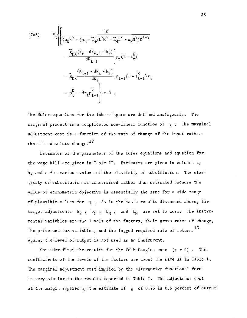
The Euler equations for the labor inputs are defined analogously. The

marginal product is a complicated non-linear function of y . The marginal

adjustment cost is a function of the rate of change of the input rather

12than the absolute change.

Estimates of the parameters of the Euler equations and equation for

the wage bill are given in Table II. Estimates are given in columns a,

b, and c for various values of the elasticity of substitution. The elas-

ticity of substitution is constrained rather than estimated because the

value of econometric objective is essentially the same for a wide range

of plausible values for y' . As in the basic results discussed above, the

target adjustments bK , bL , bN , and bH are set to zero. The instru-

mental variables are the levels of the factors, their gross rates of change,

the price and tax variables, and the lagged required rate of return.13

Again, the level of output is not used as an instrument.

Consider first the results for the Cobb-Douglas case (y = 0) . The

coefficients of the levels of the factors are about the same as in Table I.

The marginal adjustment cost implied by the alternative functional form

is very similar to the results reported in Table I. The adjustment cost

at the margin implied by the estimate of g of 0.25 is 0.6 percent of output

29

for the typical gross investment.'4 The cost is almost identical to the

estimate of 0.7 percent implicit in Table I. Again, the adjustment cost

of hours and nuither of production workers is nil while that of non-

production workers is substantial. Hence, the estimates in column a of

Table II imply the same response of the capital stock to a change in input

prices as do the basic results.

The estimates for the CES functional form are given in columns b and

c of Table II. In column b, the value of - is -0.4. In column c, it

is -1.0, which implies very low substitutability among the factors. The

results demonstrate that the marginal cost of adjustment is low, and hence

the rate of adjustment is hi-i, does not depend on the Cobb-Douglas func-

tional form. The coefficient, which determines the rate of adjust-

ment of the capital stock, remains unchanged across the wide range of

elasticities of substitution. The coefficient , which governs the

adjustment of non-production workers, only increases modestly as the

assumed elasticity of substitution decreases. The coefficients of the

levels of the inputs-- aK , aL , aN , and --do change importantly

when the assumed elasticity of substitution is varied. In particular, as

the assumed elasticity of substitution decreases the estimated marginal

productivity of labor increases and that of capital falls. Moreover, the

estimated productivity of non-production workers relative to production

workers falls as the assumed elasticity of substitution decreases. Hence,

the estimates with the low elastiëity of substitution predict relatively low

steady-state capital and non-production worker intensities. The steady-statelevel of the capital stock is ultimately determined, given the technology,

by the willingness of agents to work and supply capital. Hence, with factor

demand alone, one cannot fully characterize the level of steady-state factor

30

inputs. In any case, the estimates imply rapid adjustment of adjustment

of the capital stock to the steady state. This rapid adjustment implies

that factor price or tax policy induced changes in factor demand can be

important at business cycle frequencies.

Column d of Table II gives estimates where cost of adjustment is

presumed to be incurred only when the adjustment deviates from a target

level. The estimates are derived with the value of the targets-- bK

bL , bN , and bH --set at the sample average or the respective gross

changes in the inputs. When the targets are set to zero, adjustment cost

is presumed to occur even at very low levels of change of the factor. It

is possible, on the other hand, that only an atypical adjustment causes output

to be lost. Hence, because of the linearity of the marginal adjustment

cost, the formulation with zero targets could understate the truly marginal

adjustment cost by averaging it with the inframarginal adjustment. If

marginal adjustment cost is non-linear in this manner, then including the

target should increase the cost of adjustment coefficients. By comparing

columns a and d of Table II, one sees that the coefficients relating to the

adjustment cost change little.15 Hence, the linearity of marginal adjust-

ment cost is an adequate approximation.

Finally, I carry out another type of experiment again to determine

whether the auxiliary assumption needed to tightly restrict the data are

responsible for the conclusions. On the theoretical level, the Euler

equation for capital, (7a) or (7a'), relates the marginal product of capital

net of adjustment cost to the implied rental rate. On an empirical level,

they relate, among other things, current and lagged investment to output.

The marginal product is conveniently expressed as a function of output for

the Cobb-Douglas and CES production functions. Use of the output data allows

31

the Euler equation to be estimated even in the presence of certain unobserved

productivity shocks. Nonetheless, the use of output data invites the sug-

gestion that the estimates are only picking up the well-known accelerator.

To consider this possibility, I present the estimates in column e of Table

II. For these estimates, the output data are set to equal the mean value

for the sample. Hence, the parameter estimates cannot be attributed to a

disguised accelerator. The parameterization is the same as that in column

a, that is, y and the targets equal zero.16 The estimates with and without

the variation in the output data are very similar. The estimated is

somewhat reduced without the output data, but not by enough to alter the

major results of the paper. Hence, the strength of the results cannot be

attributed to a disguised accelerator.

A similar experiment can be carried out by likewise shutting down the

variation in the factor price and tax variables. The point of such an

exercise is to verify that identification of the parameters hinges, as the

theory suggests, on variation in factor prices. When the equations are

estimated with the factor prices at constant values, the coefficient esti-

mates change substantially.17 Specifically, when the price of capital

terms are excluded from the equations, the crucial cost of adjustment of

capital parameter, , triples. Hence, factor prices, but not output,

have an important role in identifying the coefficients of the model.

32

VI. Conclusion

This paper offers estimates of the dynamic demand for capital and labor

based on explicit considration of the firm's decision problem. The esti-

mates are based on the Euler equations. The q-theory and the linear-quadratic

approach examine closed-form decision rules of the firm. The advantage

of the Euler equation approach over the linear-quadratic approach is that

it allows more flexible functional forms and a varying and uncertain rate

of discount. The advantage of the approach over the q-theory approach is

that the adjustment cost in the Euler equation is not summarizedwith a

single, reduced-form variable.

The estimated structural parameters have reasonable values and the

capital stock responds at a credible rate to innovations in the factor

prices. These results are robust to a variety of changes in specification

of the functional form and the data. The best defense of the Euler equa-

tion approach is the plausibility of its empirical results. Specifically,

the estimates presented in this paper do not imply the excessively large

lags in the adjustmnt of the capital stock found in estimates based on

q . Therefore, the investment equation of this paper may be useful to

analyze the effects of changes in tax policy on the demand for capital.

The standard view is that rates of adjustment are so slow that the

cost of capital will not effect investment in the short run.18 To fully

study the effects of changing the cost of capital on investment would re-

quire a complete model with product demand and capital and labor supply.

Yet, the rapid rate of adjustment implied by the estimates in this paper

provides a clear challenge to the view that factor prices do not matter

for short rim fluctuations of investment.

Yale University

33

RE FERENCES

Abel, A. B., Investment and the Value of Capital (New York: Garland, 1979).

__________ "Dynamic Effects of Permanent and Temporary Tax Policies in

a q Model of Investment," Journal of Monetary Economics, IX (1982),

353-73.

__________ "Optimal Investment under Uncertainty," American Economic

Review, LXXIII (1983) , 228—33.

__________ and 0. J. Blanchard, "The Present Value of Profits and the

Cyclical Movements of Investment," National Bureau of Economic Research

Working Paper No. 1122, Cambridge, MA, 1983. Forthcoming in Econornetrica.

__________ and __________, "Investment and Sales: An Empirical Study,"

National Bureau of Economic Research Conference Paper, Cambridge, MA,

1983.

Amemiya, T., "Nonlinear Regression Models," Handbook of Econometrics, Z.

Griliches and H. D. Intrilligator, eds. (Amsterdam: North-Holland,

1983).

Arrow, K., H. B. Chenery, B. Minhas, and R. M. Solow, "Capital-Labor Sub-

stitution and Economic Efficiency," Review of Economics and Statistics,

XLIII (1961), 225—50.

Bernanke, B. S., "An Equilibrium Model of Industrial Employment, Hours,

and Earnings, 1923-1939," unpublished, Stanford University, 1983.

Berndt, E. B., and C. J. Morrison, "Income Redistribution and Employment

Effects of Rising Energy Prices," Resources and Energy, II (1979),

131—50.

Brainard, W. C., and J. Tobin, "Pitfalls in Financial Model Building,"

American Economic Review Papers and Proceedings, LVIII (1968), 99l22.

34

Brechling, F. P. R., Investment and Employment Decisions (Manchester:

Manchester University Press, 1975).

_________,and D. T. Mortenson, "Interrelated Investment and Eniployment

Decisions," unpublished, 1971.

Clark, P. K., "Investment in the l970s: Theory, Performance, and Predic-

tion," Brookings Papers on Economic Activity, No. 1 (1979), 73-113.

Epstein, L. G., and M. C. S. Denny, "The Multivariate Flexible Accelerator

Model: Its Empirical Restrictions and an Application to U.S. Manu-

facturing," Econometrica, LI (1983), 647-74.

Fair, R. C., The Short-run Demand for Workers and Hours (Amsterdam: North-

Holland Publishing Co., 1969).

Garber, P. M., and R. E. King, "Deep Structural Excavation? A Critique

of Euler Equation Methods," National Bureau of Economic Research Tech-

nical Working Paper No. 31, Cambridge, MA, 1983.

Hall, R. E., and D. W. Jorgenson, "Tax Policy and Investment Behavior,"

American Economic Review, LVII (1967), 391-414.

Hansen, L. P., "Large Sample Properties of Generalized Method of Moments

Estimators," Econometrica, L (1982), 1029—54.

__________ and T. J. Sargent, "Formulating and Estimating Dynamic Linear

Rational Expectations Models," Journal of Economic Dynamics and Control,

II (1980), 7—46.

__________ and __________, "Linear Rational Expectations Model for Dynamic-

ally Interrelated Variables," Rational Expectations and Econometric

Practice, R. E. Lucas and T. J. Sargent, eds. (Minneapolis, MN: Uni-

versity of Minnesota Press, 1982)

35

Hayashi, F., "Tobin's Marginal q and Average q : A Neoclassical Inter-

pretation,'t Econometrica, L (1982), 213-24.

Ibbotson, R. G., and R. A. Sinquefeld, Stocks, Bonds, Bills and Inflation:

The Past and the Future (Charlottesville, VA: Financial Analyst Re-

search Foundation, 1982).

Jorgenson, D. W., "Capital Theory and Investment Behavior," American

nomic Review Papers and Proceedings, LIII (1963), 247-59.

__________, and M. A. Sullivan, "Inflation and Corporate Capital Recovery,"

Depreciation, Inflation, and the Taxation of Income from Capital, C. R.

Hulten, ed. (Washington: Urban Institute, 1981).

Kennan, J., "The Estimation of Partial Adjustment Models with Rational

Expectations," Econometrica, XLVII (1979), 1441-55.

Lucas, R. E., "Optimal Investment Supply and the Flexible Accelerator,"

International Economic Review, VIII (1967), 78-85.

__________, "Econometric Policy Evaluation: A Critique," The Phillips

Curve and Labor Markets, K. Brunner and A. H. Meltzer, eds., Carnegie-

Rochester Conference of Public Policy I (Amsterdam: North-Holland, 1976).

__________, and E. C. Prescott, "Investment under Uncertainty," Econometrica,

XXXIX (1971), 659-81.

Mankiw, N. G., J. J. Rotemberg, and L. H. Summers., "Intertemporal Substitution

in Macroeconomics," Quarterly Journal of Economics, C (1985), 225-51.

Meese, R., "Dynamic Factor Demand Schedules for Labor and Capital under

Rational Expectations," Journal of Econometrics, XIV (1980), 141-58.

Morrison, C. J., and E. R. Berndt, "Short-run Labor Productivity in a Dynamic

Model," Journal of Econometrics, XVI (1981), 339-65.

Nadiri, M. I. , and S. Rosen, "Interrelated Factor Demand Functions,"

American Economic Review, LIX (1969), 457-71.

36

Pindyck, R. S., and J. J. Rotertherg, "Dynamic Factor Demands under Rational

Expectations," Scandinavian Journal of Economics, LXXXV (1985) 223-38.

Rotemberg, J. J., "Interpreting the Statistical Failures of Some Rational

Expectations Macroeconomic Models," American Economic Review Papers

and Proceedings, LXXIV (1984) , 188-93.

Sargent, T. J., "Estimation of Dynamic Labor Demand Schedules under Rational

Expectations," Journal of Political Economy, LXXXVI (1978), 1009—44.

Summers, L. H., "Taxation and Corporate Investment: A q-Theory Approach,"

Brookings Papers on Economic Activity, No. 1 (1981), 67-127.

Survey of Current Business, U.S. Department of Conimerce, Bureau of Economic

Analysis, various nuithers.

Tobin, J. "A General Equilibrium Approach to Monetary Theory," Journal

of Money, Credit and Banking, I (1969), 15-29.

_______, and P. M. White, "Comments and Discussion," Brookings Papers

on Economic Activity, No. 1 (1981), 132-39.

Treadway, A. B., "On the Multivariate Flexible Accelerator," Econometrica,

XXXIX (1971), 845-55.

37

FOOTNOTES

*This paper is a revision of Chapter One of my 1984 M.I.T. Ph.D dis-

sertation. I am grateful to my committee, Stanley Fischer, Jerry Hausman,

and Olivier Blanchard, and to Andrew Abel, Ernst Berndt, N. Gregory tankiw,

James Poterba, David Romer, Julio Rotemberg, Lawrence Summers, numerous

seminar participants, and anonymous referees for their extensive comments

and discussion. I gratefully acknowledge the financial support of the

National Science Foundation and the Social Science Research Council Sub-

committee on 4onetary Research.

1. Hayashi [1982] shows that average q equals marginal q under

certain circumstances such as constant returns to scale.

2. The cost of intermediate inputs do not appear in the expression

for profits so real value added minus real factor costs equals real profits.

3. Sargent [1978] and Meese [1980] use a quadratic production function

and do not impose or test CR5 or convexity. Pindyck and Rotemberg [1983] im-

pose and test CRS and convexity when estimating a trans-log cost function.

Morrison and Berndt [1981] show how to impose CRS in a quadratic cost func-

tion. I tried a trans-log specification but failed to identify the produc-

tion function parameters. In some cases the parameter of the first-order

term in Lt exceeded one. It is difficult to untangle the adjustment

cost parameters from the other production function parameters in the trans-

log case because they both multiply second-order terms in the factors.

4. I consider specifications where the overtime premium is asymmetric

so it is paid only when hours exceed 40. The data strongly do not reject

symmetry. In aggregate data some overtime is always paid; a symmetric

premium appears to be a good approximation.

5. I use the quarterly PVCCA and ITC constructed by Data Resources,

Inc.

38

6. The compensation data are annual. I interpolate to obtain quarterly

data. Because separate data are not available, the same quit rate is used

for production and non-production workers.

7. I carried Out the estimation in a FORTRAN program which I wrote

to perform GMM. The program will handle general, non-linear problems.

8. Rotemberg [1984] argues that if the overidentifying restrictions fail,

different instrument lists could lead to vastly different estimates. That

the estimates remain essentially unchanged when the timing of the instru-

ments is changed is informal evidence that his problem does not arise with

these estimates even though the J statistic is large.

9. To calculate the root, I must make more explicit assumptions about

the environment of the representative firm than in the Euler equations. With

the Euler equations, I assume that the representative firm is a price

taker. It would be incorrect, however, to assume that there is no feed-

back from factor and product markets to the representative firm. Even

if the market is competitive, the representative firm will move down the

market demand curve arid up the labor supply curve. The competitive assump-

tion means only that the firm does not take its effect on prices into ac-

count in its decision rule. I assume that labor is supplied inelastically,

so Lt , Nt , and are held constant. Wages relative to output prices

are also held constant. Summers [1981] makes a similar assumption.

Using parameter values from Table 1, column b, the linearized rule for

representative form is

Kt = 0.75 Kti - 7.1O.93'(Etpi - drEP.1)

when the required rate of return is constant.

39

10. .1eese [1980, p. 151], using the technique advocated by Hansen and

Sargent [1980, 1982] estimates that the root in the capital equation is 0.9563.

Again, the adjustment lags are much larger than in my estimates, but not

as large as in Summers. The root of 0.9563 implies that half the adjust-

ment to the steady state takesplace after four years. Moreover, it takes

the economy over 25 years to get within one percent of the steady state

under Meese's estimate compared to four years under the estimates presented

here.

11. The limiting argument is a straight-forward application of

L'H6pital's rule.

12. A term with the square of the level of capital in the denominator

arises from differentiating the lead expression of the production function

by the current capital stock. This term is two orders of magnitude smaller

than the other terms in the Euler equation and hence has negligible numeri-

cal effect on any of the calculations. Consequently, it is omitted from

(7a') and the other Euler equations.

13. Because use of the GMM estimates did not alter any conclusions

for the results in Table I, only the three-stage least squares estimates

are given here. The values of the three-stage least squares objective

M for the parameter estimates given in Table I are similar to those given

in Table II for the alternative estimates.

14. Over the sample period, the average quarterly rate of gross change

of K is 2.4 percent, of L is 6.2 percent, of N is 6.6 percent, and

of H is -0.01 percent.

15. The estimate in column d presumes y equal to zero. Similar

results hold for other values of that parameter.

16. The conclusions of this paragraph are unaltered for estimates for

other elasticities of substitution and for the non-zero values of the targets.

40

17. The exceptions are aL and aN , which are still tied down by

the factor intensities. On the other hand, , which depends on the

wage function, and coefficients relating to the wage function and cost

of adjustment change substantially and nonscenically.

18. The standard view of the effect of the cost of capital on invest-

ment is well-represented by the following:

The effect of interest rates and tax changes.. .are

likely to be felt only gradually, over long periodsof time. For short-term forecasting (two years orless), the effect of moderate variations in taxesand interest rates is likely to be negligible.

(Clark [1979, p. 104])

TABLE I

Estimates of the First-Order Conditions (7)

and Equation for the Wage Bill (4)

1955 QIlI to 1980 QIlI

(a)InstrumentsCurrent

(b)

Lagged(c)

Current(d)

Lagged

w0 1.49 1.50 1.50 1.50(0.02) (0.02) (0.02) (0.02)(0.06) (0.08) (0.06) (0.08)

0.43 0.43 0.43 0.43(0.02) (0.02) (0.02) (0.02)(0.05) (0.06) (0.05) (0.09)

w2 —0.05 —0.05 —0.05 —0.05(0.006) (0.006) (0.007) (0.008)(0.011) (0.020) (0.018) (0.023)

aL 0.45 0.46 0.46 0.46(0.005) (0.005) (0.006) (0.006)(0.009) (0.009) (0.017) (0.018)

aN 0.27 0.27 0.27 0.27(0.004) (0.003) (0.004) (0.004)(0.007) (0.009) (0.017) (0.014)

a 0.53 0,53 0.52 0.52H(0.01) (0.01) (0.0l1 (0,011)(0.02) (0.02) (0.022) (0.028)

0.0013 0.0014 0.0011 0.0014(0.0004) (0.0006) (0.0005) (0.0005)(0.0011) (0.0014) (0.0014) (0.0020)

-0.0002 -0.0003 0.0007 0.0006(0.0008) (0.0010) (0.0016) (0.0023)(0.0018) (0.0030) (0.0043) (0.0088)

0.088 0.088 0.088 0,088(0.027) (0.023) (0.039) (0.047)(0.097) (0.062) (0.193) (0.23)

0.00047 -0.0001 0.0007 0.0003(0.00027) (0.0005) (0.0005) (0.0006)(0.00068) (0.0019) (0.0012) (0.0025)

0.0010 0.0010(0.0004) (0.0005)(0.0012) (0.0019)

continued...

41

TABLE I (continued)

Instruments (a)

Current(b)

Lagged(c)

Current(d)

Lagged

g -0.0005

(0.0021)(0.0083)

-0.0006

(0.0025)(0.0011)

g -0.0003

(0.0003)(0.0009)

-0.0007(0.0004)(0.0014)

0.0005

(0.0044)(0.017)

0.0008(0.0074)(0.038)

g 0.0004

(0.0007)

(0.0017)

0.0011

(0.0011)(0.0035)

g 0.0008

(0.0020)(0.0080)

0.0006

(0.0040)(0.014)

J* 103.3 104.6 104.1 103.9

Significance 0.017 0.014 0.004 0.004

Standard errors in parentheses. The first standard errors are from3SLS, the second from GMM.

J test of overidentifying restrictions (see Hansen [1982]). J isdistributed as chi-squared (85-k) where k is the number of parametersestimated. It is here calculated using the GNM rather than the leastsquares objective.

42

TABLE II

Parameter Estimates under Alternative Assumptions

(a)

targets =0

(b)

targets =0

(c)

targets =0

(d) (e)

targets =0;targets = means output data

= mean

0.0 -0.4 -1.0 0.0 0.0

w0 1.50 1.50 1.50 1.50 1.51(0.02) (0.02) (0.02) (0.02) (0.02)

w. 0.33 0.32 0.31 0.33 0.33-(0.02) (0.02) (0.02) (0.02) (0.02)

w2 —0.02 —0.02 —0.01 —0.02 -0.02(0.005) (0.003) (0.009) (0.005) (0.005)

0.26 0.25 0.16 0.26 0.26(0.01) (0.01) (0.01) (0.01) (0.01)

aL 0.47 0.69 0.83 0.47 0.46(0.01) (0.01) (0.01) (0.01) (0.01)

aN 0.27 0.06 <0.005 0.27 0.28(0.003) (0.001) (<0.0005) (0.003) (0.004)

0.05 0.02 <0.005 0.05 0.05(0.01) (0.002) (<0.0005) (0.01) (0.01)

0.25 0.25 025 0.25 0.21(0.08) (0.08) (0.08) (0.05) (0.04)

—0.01 —0.01 —0.01 —0.01 —0.01(0.01) (0.01) (0.02) (0.01) (0.01)

0.23 0.27 0.34 0.23 0.23(0.07) (0.08) (0.09) (0.07) (0.06)

0.002 <0.0005 <0.0005 0.002 —0.01(0.007) (<0.00005) (<0.00005) (0.007) (0.006)

M 305 305 309 304 297

Three stage least-squares standard errors in parentheses. M is thevalue of the three-stage least squares objective.

In columns a, b, c, and e, the target coefficients-- bK , bLbN , and b11 --are zero. In columii d, they are equal to the sample means

of the gross changes in the factors. In colunui e, the output data are con-strained to equal the mean value.

43