NBER WORKING PAPER SERIES

THE EVOLUTION OF PUBLICSECTOR BARGAINING LAWS

Henry S. Farber

Working Paper No. 2361

NATIONAL BUREAU OF ECONOMIC RESEARCH1050 Massachusetts Avenue

Cambridge, MA 02138August 1987

An earlier version of this paper was prepared for the NBER Conference on PublicSector Unionism in Cambridge, Massachusetts, August 15-16, 1986. Gregory Leonardand Robin Maury provided research assistance. The author thanks John Abowd forvery helpful discussions and Robert Valletta for help with the NBER public sectorbargaining law data set. Useful comments on an earlier draft were provided byCasey Ichniowski and Edward Lazear. Support from the Sloan Foundation is gratefullyacknowledged. The research reported here is part of the NBER's research programin Labor Studies. Any opinions expressed are those of the author and not thoseof the National Bureau of Economic Research.

NBER Working Paper #2361August 1987

The Evolution of Public Sector Bargaining Laws

ABSTRACT

In 1955 only a few states had laws governing collective bargaining bypublic employees. By 1984 only a few states were without such laws. Theemergence of these policies coincides with a dramatic increase in unionizationamong public employees, and an important puzzle is the direction of causalitybetween the laws and public employee unionization. A key piece of thesolution is understanding the evolution of the public policy in this area, andthis is the focus of the analysis in this study.

A Narkov model of the evolution of these laws is developed based on theidea that states will change their existing policy if and only if theirpreferences deviate from the existing policy by more than the cost of a changein policy. The key underlying constructs are 1) the intensity of statepreferences for or against public sector collective bargaining and 2) the costof changing an existing policy or enacting a new policy. The model isimplemented empirically using state level data on policy for each year from1955 to1984. The results suggest that state preferences for a pro—bargainingpolicy are positively related to 1) the COPE score (a measure of pro—unioncongressional voting behavior on labor issues), 2) income per capita, and 3)the size of the public sector and negatively related to southern region. Thecosts of policy change were hypothesized to be a function of structuralmeasures of the legislative process, but no support for this was found in thedata. Use of the estimates to predict probabilities of states having laws ofvarious kinds suggests that the model can predict the aggregate distributionof laws relatively well but that the model does less well at distinguishingbetween states with laws of different types.

Henry S. FarberDepartment of EconomicsMITE52—252FCambridge, MA 02139

1

I. Introduction

It has been argued that the tremendous increase in collective bargaining

among state and local government employees is largely the result of the

passage of laws by states sanctioning and regulating the process of collective

bargaining by government employees.' In 1955 less than a handful of states

had laws defining the collective bargaining rights of public employees and

virtually all of these prohibited bargaining. By 1984, all but a few states

had adopted a policy in this area, and only a handful of states prohibited

bargaining. Table 1 contains a breakdown of state laws governing the

collective bargaining rights of public sector employees in 1955 and 1984

derived from the the NBER public sector bargaining law data set (Valletta and

Freeman, 1986). While there are serious problems of causal inference in

concluding that the emergence of public policy caused the increase in

unionization, the emergence of public policy in this this area along with

public sector unionization represents an important puzzle for industrial

relations scholars. If the public policy did cause the the increase in

unionization then the problem is to explain the emergence of the public

policy. If unionization (or the pressure for unionization) resulted in public

policy to deal with it then the problem is to explain the emergence of the

unionization.

The ideal would be to specify and estimate a full structural model of

the determination of public sector legislation and unionization that afforded

the opportunity to determine the direction of causality directly. However,

estimation of such a model would strain the limits of the available data and

'Freeman (1986) makes this argument directly in the context of an interestingsurvey of the growth of unionism in the public sector. See also the work ofReid and Kurth (1983), Dalton (1982) , Noore (1977) , Ichniowski (1988), andLauer (1979)

Table 1:

Number of States With Laws Governing Collective Bargaining Rigs

1955° 1984

No Law Law No Law Law

State Employees 44 4 8 42

Police 45 3 8 42

Teachers 45 3 3 47

°There were only 48 states in 1955.

Source: NBER public sector bargaining law data set. Valletta and Freeman,1986.

2

econometric technique. A difficult, if somewhat less ambitious, task is

undertaken in this study: the specification and estimation of a reduced form

model of the determination of state laws governing public sector bargaining.2

The analysis is reduced form in that the direct effect of public sector

unionization on public policy is not analyzed, and it is argued that the

public policy is a function of the combined sets of factors that affect public

policy indirectly through their effect on public sector unionization as well

as the factors that affect public policy directly.

The empirical analysis relies on the NBER public sector bargaining law

data set (Valletta and Freeman, 1986) which contains information on each

states' laws governing collective bargaining by public sector employees for

each year in the 1955—1984 period. Information is available separately for

laws governing each of five classes of employees (state employees, local

police, fire, teachers, and other local employees). The analysis here deals

with state employees, police, and teachers as groups that are representative

of public employees more generally and capture the important variation in laws

3across employee groups. While a number of different aspects of each law are

summarized in the data (e.g., collective bargaining rights, union security

provisions, policy regarding strikes, alternative dispute settlement

mechanisms), the analysis focuses on the fundamental policy regarding

collective bargaining rights. This can range from a prohibition on bargaining

to a requirement that public sector employers bargain with their employees.

2Kochan (1973), Faber and Martin (1979), and Saltzman (1985) present studiesof the determinants of public sector bargaining laws.

3For example, both police and firemen are viewed as critical local governmentemployees, and the public policy issues raised by unionization of these groupsare similar.

3

These data are described more fully in the next section.

In section III a model of the determination of the passage of

legislation governing public sector collective bargaining is developed. This

model describes the process that governs states' decisions regarding 1)

whether or not to enact a law governing public sector bargaining rights, 2)

what type of policy to enact if a law is passed, 3) whether or not to change

an existing policy, and 4) what type of policy to change to if a change is

passed. The model is based on two central constructs. The first is intensity

of preferences for or against public sector unionization and the second is the

cost (ease or difficulty) of enacting or changing public policy in this area.

Essentially, it is argued that a state will enact a policy or change its

existing policy if their preferences differ from the value of the current

policy (or no policy) by enough to outweigh the costs of the change.

The econometric framework is outlined in section IV. A Markov model of

transitions from one category of law to another category (or from no law to a

particular type of law) conditional on the initial category is specified. The

transition probabilities are derived directly from the theoretical framework

developed in section III.

An important part of the estimation of the model is to identify the

factors that influence the intensity of preferences for public sector

unionization and the costs of policy change. Section V contains descriptions

of the explanatory variables used to measure variation in the costs associated

with the legislative process. These include the number of days the state

legislature meets, a measure of general legislative activity, an indicator of

whether or not the legislature and the governorship are controlled by the

same party, and a time trend. Section VI contains descriptions of the

explanatory variables used to measure variation in intensity of preferences.

These include congressional voting records on labor issues, private sector

4

unionization, income per capita, the relative size of the government sector, a

time trend, and regional factors. The same set of variables is argued to

measure variation in the value to a state of having no explicit policy.

The empirical results are presented in section VII. The most important

factors found to be influencing the intensity of preferences for public sector

unionization are the congressional voting records, southern region, income per

capita, and the size of the government sector. Nothing measured in this study

is found to influence the costs legislative change in a systematic fashion.

Section VIII contains an investigation of how well the model fits the data.

It is found that the model can explain the overall distribution of laws at

various points in time rather well. However, the model is less successful in

explaining which states have laws of a particular kind at each point in time.

In section IX the results are summarized, and it is concluded that the model

of legislative change developed in this study has some explanatory power but

that more work needs to be done in defining and measuring variables that

affect the costs of legislative change and preferences for public sector

collective bargaining.

II. Des cripion of Bargaining Law Data

The National Bureau of Economic Research public sector bargaining law

data set, described in detail by Valletta and Freeman (1986) , contains a

record of the legislative history of each state's policy regarding public

sector collective bargaining. In constructing these data, a serious attempt

was also made to incorporate policies toward public sector collective

bargaining that originated from judicial decisions. However, because most

existing policy in this area has a legislative foundation and because the

measurement of judicially made policy is likely to be incomplete, the data can

5

be thought of as representing a largely legislative history.4 On this basis

the analysis that follows is developed in terms of policy as being derived

through a legislative process.

Overall, these data represent the best available comprehensive source of

quantitative information on policy regarding public sector collective

bargaining. The data are compiled separately for laws covering the three

employee groups focused on here: state employees, police, and school teachers,

and for each group information is collected regarding public policy governing

their collective bargaining rights.

Since it is not possible to characterize parsimoniously the specifics of

every law with respect to collective bargaining rights, the laws are

categorized with regard to their general content. Four types of laws are

defined ranging from the least favorable for bargaining to the most favorable.

The categories are defined in table 2. In the least favorable category,

bargaining is prohibited while in the most favorable category the employer is

obligated to bargain with the union. In the two intermediate categories

bargaining is more—or—less optional.

The evolution of laws governing collective bargaining rights of public

sector employees is quite dramatic. Table 3 contains a breakdown of laws

governing collective bargaining rights by state for each of the three employee

groups in 1955 and 1984. It is clear that in the mid—1950's very few states

had any policy at all regarding collective bargaining rights for public sector

employees, and the laws in those states that did have a policy were not

Incomplete measurement of judicially based policy should be more of aproblem in the early years prior to the passage of legislation because, at

that time, the courts could exercise discretion without reference to specificlegislation.

Table 2:

Categories of Laws Govern Collective Bargaining Rights

TY

0 No Legislative Policy

1 Bargaining prohibited

2 Employer permitted but not obligatedto negotiate with union

3 Union has right to present proposalsand/or meet with employer

4 Employer has duty to bargain withunion

6

favorable to collective bargaining. By 1984 the large majority of states had

adopted a policy, and these policies were largely favorable to collective

bargaining. For all three employee groups, approximately half of the fifty

states had adopted a policy of requiring employers to bargain with their

employee's unions. While the frequency distributions of type of policy in

1984 are relatively close for the three employee groups, public policy is more

favorable for bargaining on average for teachers than for the other two groups

and somewhat more favorable for police than for state employees. In 1984 more

states had laws requiring bargaining and fewer laws prohibiting bargaining

with teachers than with the other two groups. Similarly, more states had laws

requiring bargaining with police than with state employees.

If we consider each year in a given state to be an opportunity for the

state to modify its public policy, then there are a total of 1490 observations

on the evolutionary process for each of the three employee groups.5 Table 4

contains breakdowns of these processes in the form of cross—tabulations by

employee group of the current year's legislative category by the previous

year's legislative category. What is obvious is that for all groups most of

the 1490 observations are on the diagonals, meaning that there is generally no

change in policy. In fact, of the 1490 opportunities to change policy,

changes occurred only 52 times for state employees, 52 times for police, and

61 times for teachers.

Of the 52 changes in policy regarding state employees, 39 of these were

initial enactments of a policy, 6 of which prohibited bargaining. Of the 13

5There are not 30x50=1500 observations because Alaska and Hawaii did notbecome states until 1959 and 1960. Thus, these states do not contributeobservations for the five year period from 1955 to 1959, resulting in tenfewer observations.

Table 3:

Breakdown of laws governing Collective Bargaining Rights by CategoryC

Po Teachers

1955 1984 1955 1984 1955 1984

NoLaw 44 8 45 8 45 3

1 3 8 2 4 2 4

2 1 6 1 9 1 12

3 0 4 0 2 0 1

4 0 24 0 27 0 30

'There are only 48 states in 1955. See Table 2 for category definitions.

Source: NBER public sector bargaining law data set. Valletta and Freeman,1986.

7

6changes in an existing policy, all involved a change to a more favorable law.

Of the 52 changes in policy regarding police, 40 of these were initial

enactments of a policy, 4 of which prohibited bargaining. Of the 12 changes

in an existing policy, all but one involved a change to a more favorable law.

Of the 61 changes in policy regarding state employees, 45 of these were

initial enactments of a policy, 3 of which prohibited bargaining. Of the 16

changes in an existing policy, all but 2 involved a change to a more favorable

law.

Since most of the "action" is in the initial implementation of a public

policy regarding bargaining, an important focus of the analysis is on the

pattern of emergence of these policies, both across states and over time.

There is also a significant amount of change to existing policy that must be

accounted for. However, the dominant set of observations consists of those

where policy is unchanged, and the theoretical and empirical framework must

be able to accommodate this fact.

III. Theoretical Framework

A simple model of the passage of legislation governing public sector

collective bargaining relies on two factors. First, the intensity of

preferences for or against public sector unionism is an important determinant

both of the passage of any law and the particular type of law passed. Where

preferences in a state are very favorable toward unionization, the state will

be more likely to have a prouniori bargaining law. Similarly, where

preferences in a state are very unfavorable toward unions, the state will be

6For state employees, only Florida first prohibited bargaining (category 1)then moved to a policy requiring bargaining (category 4). For police, onlyNevada and Texas had such a reversal of policy. For teachers, only Nevada hadsuch a reversal of policy.

Table 4:Cross—tabulation of Current Collective Bargaining Policy

by Previous Year's Policy

S Employees

LaggedPolicy Current Policy

0 1 2 3 4

0 748 6 13 8 12

1 0 169 0 0 1

2 0 0 127 1 6

3 0 0 0 96 5

4 0 0 0 0 298

Police

LaggedPolicy Current Policy

0 1 2 3 4

0 742 4 14 5 17

1 0 89 1 0 2

2 0 1 191 0 5

3 0 0 0 47 3

4 0 0 0 0 369

Teachers

LaggedPolicy Current Policy

0 1 2 3 4

0 657 3 18 5 19

1 0 89 2 0 1

2 0 2 233 1 5

3 0 0 0 50 5

4 0 0 0 0 400

°See Table 2 for category definitions.

8

more likely to have an anti—union bargaining law. The second factor is the

difficulty of passing legislation independent of the intensity of preferences

for or against unionization. This difficulty level is termed the costs of

enacting legislation, and it is argued to be largely a function of the

structure of the legislative process. A key feature of the model is the

independent nature of the intensity and the costs. Any factors that affect

the difficulty of passing legislation in a way that is related to intensity

are subsumed in the intensity measure.7

Suppose that a law governing the collective bargaining rights of public

sector employees can be characterized along a single dimension and that the

optimal value of a law (intensity of preference) in this dimension is denoted

by R. in state i and year t. A higher value for denotes preferences that

are more favorable toward bargaining. Suppose further that a loss function

L. with regard to collective bargaining policy can be defined simply as the

absolute value of the deviation of the value (V) of the current policy, j,

from the optimal value, R,. This loss function is

(111.1) L. = IR. '. I.it it jIf it was costless to enact a policy or change an existing policy then in each

period each state would minimize L. by choosing j such that In other

words, the policy each period would reflect the currently optimal policy.

However, it is generally costly to introduce a new policy or to change an

existing policy due to friction in the political process.

7it is clear that the empirical analysis of outcomes will not support anyother interpretation. For example, anything that makes it more likely that afavorable law is passed cannot be classified unambiguously as more favorablepreferences as opposed to lower costs of passing favorable legislation. Theanalogous argument can be made for unfavorable legislation.

9

Consider first the case where a state has no policy in place. How will

that state decide whether to introduce policy or to remain without a policy?

Denote the value of no policy by V0.,, so that the loss function evaluated at

no policy is simply

(111.2) L. = IR. — V .it,O it OitIf the cost of introducing a policy is C. then the state will find it optimal

to introduce a policy only if the loss from introducing the law (C.) is

smaller than the benefit derived from elimination of the loss from no policy.

This condition is

(111.3) IR.— V

.> C.it Oit it

assuming that the state is able to introduce a policy that has a zero loss

8associated with it (V,R. ).

j ii.Note that this formulation does not impose a particular value to "no

policy" relative to the actual policies. The value of no policy has state

and time subscripts because there is generally a de facto policy implicit in

no official policy that is likely to be state specific and change over time.

For example, no official policy in a generally prounion state will have a

different value than no official policy in a generally antiunion state.

The available data group the laws into the discrete categories defined

in table 2. In order to derive the decision rules for states that have an

existing policy, define V. as the value of a law in category j. Given the

definition of the four categories (excluding no policy) in table 2, it is

natural to assume that V1 <V2 (V3 (V4.

This is not a terribly realistic assumption, and it is not consistent withthe empirical analysis that follows. However, it simplifies the analysisquite a bit without changing its fundamental nature.

Start with #3:

Start with #4:

9Such a retreat is never observed.

interpreted as the point of

category 2, and as long as

by enough to outweigh the cost of

policy. It is not necessarily true

condition holds. This condition

state to desire a change to one of

each of the policy categories are derived

< K — C. or R. ) K + C and

R. <K —C.it 3 it

10

Once a state has a policy in place, it is assumed that this policy can

be maintained costlessly but that a change in policy entails incurring some

level of costs, C., that is independent of the particular policy in place.

In this case a state will decide to change its old policy if and only if the

loss associated with the current policy is greater than the loss associated

with the the best alternative policy plus the cost of change. It is further

assumed that a state cannot retreat to having no explicit policy regarding

public sector collective bargaining once a policy is enacted.9

Using the same notation as above, a state with a category 1 law

(prohibiting bargaining) will want to change that law if

(111.4) R. > K + C.it I itwhere K1 = (V1+V2)/2. The value can be

indifference (in R) between category 1 and

preferences exceed this indifference point

the change, then the state will change its

that the state will adopt policy 2 if this

is simply necessary and sufficient for the

the other (higher) categories.

The conditions to move from

similarly and are:

Start with #1:

Start with #2:

(111.5)

R. )K +Cit 1 i4..

R <K —C orR >K +Cit 1. it it 2 it

11

where

K1 = (V1-f-V2)/2,

(111.6) K2 = (V2+V )/2, and

K3 = (V3+V4)/2.

If the appropriate inequality conditional on the initial policy is not

satisfied then the state will retain its existing policy. If the appropriate

inequality is satisfied so that the state decides to change its policy, the

state will move to the category that yields the lowest value for the loss

function.

Given that a state decides to enact a new policy or to change its

existing policy, the state will use a similar decision rule in selecting the

optimal category of law. The loss function is minimized by selecting the

category of law whose value is closest to R1. The category of law that

minimizes the loss function is defined by the interval on the real line

delimited by the K1 that R. falls in. For example, the lowest value law

(category 1) will be chosen if < K1 where K1(V1+V2)/2. Similarly, they

will choose category 2 if K1(R.<K2 where K2=(V2+V3)/2. The complete set of

conditions is

Choose 1 if: R. ( K1. 1

Choose 2 if: K ( R. < KI it. 2

(111.7)Choose 3 if: K < R. < K , and

2 it. 3

Choose 4 if: R, > Kit. 3,

where the breakpoints are defined in equation 111.6.

There are two key features of this model from the standpoint of the

empirical analysis carried out in succeeding sections. First is that the

12

model allows the central construct of intensity of preferences (R.) to affect

three important elements of the evolution of public policy regarding

collective bargaining in the public sector: 1) the process that determines

whether a state has a policy at all, 2) the process that determines whether

the state adjusts its law to reflect current conditions, and 3) the particular

kind of law that is adopted in an ordered response context. The second key

feature of the model is that the central construct of costs of adjustment

(C.) makes it is possible for changes in policy to be relatively rare events.

This is because the costs of policy change will provide a disincentive to

change policy in response to small changes in preferences.

IV. Econometric Specification

The basic approach taken to the econometric specification is to assume

that there are 1490 (48 states x 30 years ÷ 2 states x 25 years) observations

for each employee group on the current state of policy regarding public sector

collective bargaining rights conditional on the policy that prevailed at the

end of the previous year. Thus, the probabilities of having a particular

policy in a given state—year are specified conditional on the previous policy,

and. these probabilities are used to form a likelihood function that is

maximized with respect to a set of underlying parameters that are common to

the various conditioning events.

The econometric framework used for this task is an extension of a

standard ordered probit model. Conditional on the previous policy (or no

policy) , the specification will indicate the probability of the joint event of

1) change or no change in that policy and 2) choice of the particular policy

that was implemented where there was a change. This is essentially a Markov

model of the transition probabilities based on the frequencies in table 4.

The contribution of the theory is that it provides a way to specify each of

13

the transition probabilities in this matrix as a function of the same set of

underlying parameters and in terms of a coherent model.

Equations 111.5 — 111.7 define the decision rules that determine whether

or not a state will enact or change policy and what sort of policy will be

enacted if there is a change. These depend on the values of the cost of

changing policy (C) the intensity of preference (R). the value of no

policy ('1. )' and the threshold values (K1, K2, and K3).

The cost of changing policy (C.) is a fundamentally unmeasurable

quantity that is modeled empirically as the latent variable Y1 for a given

observation where1°

(IV.1) Y1 =X1/31 +&.

The vector represents observable variables that affect the cost of policy

change, is a vector of parameters, and E is a random component.

Similarly, intensity of preferences (R.) is a fundamentally unobservable

quantity that is modeled empirically as the latent variable Y2 for a given

observation where

(IV.2) y, =x2i3 +e2.

The vector X represents observable variables that affect the intensity of

preferences, 2is a vector of parameters, and

2is a random component. A

third underlying construct is the value of no policy (V0.). This is

specified simply as

(IV.3) Y3 =x3133

where the vector X represents observable variables that affect the value of

no policy and /33 is a vector of parameters. There is no stochastic element in

10The "it" subscripts are suppressed in this presentation, except wherenecessary for clarity, to keep the notation uncluttered.

14

this construct.

The particular variables in the X vectors are discussed in the next

section. It is assumed that and E have independent standard normal

distributions. Given the qualitative nature of the outcomes, it is not

possible to identify the variances or 2 together with the scale of /3, /3,

and /33. Thus, the variances are normalized to one. The means of C and C2

are normalized to zero because systematic unobservable factors are subsumed

in the constant terms in X1131, X2132, and X3/33. The zero correlation

restriction is imposed for analytical convenience, but it is consistent with

the argument made in section III that the factors affecting intensity of

preferences and costs of policy change are independent by construction.

Given these specifications for the costs of policy change, the intensity

of preferences, and the value of no policy along with the model outlined in

the previous section, it is possible to write the probabilities of all

possible outcomes for each of the conditioning sets (initial policies). Let

J represent the type of law in place in state i in year t. The index can

take on any of the five values 0,1,2,3,4 where 0 represents no policy and 1

through 4 represent the four categories of collective bargaining rights law

described in table 2. These are the five conditioning events that define the

five rows of the Markov transition matrix. The transition probabilities are

defined as

(IV.4) P = Pr(J =! =m) for n,m = 1 ...5mnt L t—1

where represents the probability that a state with law category m in

year t—1 has law category n in year t. These probabilities sum to one for

each conditioning event such that4

(IV.5) V p = 1 m = 0,1,2,3,4.n= 0

The various P depend on the same set of parameters and are defined in

15

11detail in the Appendix.

It is straightforward to formulate the likelihood function for this

model based on the probabilities for the various events outlined in this

section and presented in the appendix. The associated log—likelihood function

is

(IV.6) ln(L) =

84

I ln(Pmnxt, mn4.,=55 i1 m0 n0

where I is an indicator variable that equals one if state i had law m inmnit

year t—1 and law n in year t. The variable I equals 0 otherwise.12mn.I t.

Computation of this likelihood function involves evaluation of nothing more

complex than bivariate normal CDF's, and these are readily computable using

numerical approximations. The empirical analysis consists of maximization of

this likelihood function with respect to the free parameters of the model

•2'3 K1,K2,andIC3).

One shortcoming of the Markov approach used here and implicit in the

likelihood function is that it assumes there is no correlation across time and

within states in the errors and2' It is certainly likely to be true that

there are persistent unmeasured factors that affect the intensity of

preferences and the costs of policy change within states. However,the

appropriate technique for dealing with this problem is not clear. A fixed

effect estimator, which includes a separate intercept for each state (perhaps

While the derivations of the probabilities are straightforward, they makerather tedious reading. The reader may find it useful to examine thederivation of a few of the probabilities in the appendix in order to be clearabout their nature.

12The variable I = 0 for all values of in and n for Alaska and Hawaii priormnj. tto 1960.

16

in Y , Y2, and Y3) imposes too high a computational burden in a nonlinear

model such as this. It also strains the limits of the information in the

data. There are also difficult computational problems in using a random

effects estimator.

While this section in conjunction with the appendix contains much

tedious specification of probabilities, the overall structure of the two

equation model is clear. States will change their policy if their

preference/cost structure changes so that a different policy is optimal net of

the costs of the change. The policy that states will select if they do opt to

change will be the option closest to their most preferred position. In the

next two sections the observable variables that determine the cost of policy

change, the intensity of preference, and the value of no policy are described.

V. The Costs of a Change in Public Policy

The costs of a change in public policy is a construct designed to

capture how difficult it is to make a legislative change in policy. An

important determinant of this is the structural makeup of the state

government. While it is unclear exactly what organizational or political

factors lead to higher or lower difficulty in implementing legislative change,

three measures that are likely to reflect these underlying factors are used in

this study.

The first is the number of days the state legislature is in session.

The argument is that a legislature in session more days has a greater chance

of passing a given piece of legislation. In addition, a legislature that

meets frequently is argued to exhibit more professionalism. It should also be

noted that a number of states had legislative sessions only every other year

or had only perfunctory sessions every other year until recently. It is clear

that these states are unlikely to pass important legislation in the "off"

17

years, and a variable representing days in session will capture this

phenomenon. The measure of legislative days was not available for 1983 and

1984, and the 1982 figure for each state was used for these years. The mean

and standard deviation of this variable and the others discussed in this and

the next section are contained in table 5.

The second variable used is the number of bills enacted by the state

government (passed by the legislature and signed by the governor). The

arguments used to justify this variable are similar to those for the number of

days the legislature is in session. The data on number of enactments was

missing for a few observations, and values for these observations were imputed

by interpolation from adjacent years.13

The final legislative structure variable used is a dummy variable that

reflects whether or not the state legislature and the governorship are

controlled by the same party. It is argued that where there is this unified

control, the government will be able to achieve whatever it wants more easily.

This could be favorable or unfavorable bargaining legislation.14

A time trend measured by year is included in the cost function in order

to capture any secular change in the difficulty of legislative change in this

area. One argument for such a change is that as the public sector grew over

this period and/or as public sector workers became more interested in

unionization, the general pressure to articulate some policy with regard to

13Data for 1955 and 1957 for New Jersey and for 1955 for New York were missing.

14There were nonpartisan elections in Nebraska for the entire period and inMinnesota for part of the period. Given the absence of a party structure, theconcept of unified control has little meaning so the dummy variable was-assigned a value of zero in these cases.

18

public sector collective bargaining grew. That the pressure is not

particularly for a positive or a negative policy, but simply for some policy,

suggests that this factor belongs in the cost equation where a negative

coefficient would indicate an increase over time in the likelihood of a change

in policy.

VI. Intensity of Preferences for Public Sector Collective Bargaining and the

!L P1cY

Perhaps the most important factor that would influence a state with

regard to policy toward collective bargaining by public sector employees is

the general attitude toward unions in the state. Three variables are used

here to reflect these attitudes. The first is a measure of the "liberalness"

on labor issues of the congressional delegation of the state. This is likely

to be important to the extent that 1) congressmen reflect the preferences of

the voters in their states on labor issues and 2) these voters elect state

legislators who also reflect these same attitudes. The measure used is the

"COPE score" of the congressional delegation of the state. The Committee on

Political Education (COPE) and the legislative department of the AFL—CIO

regularly tabulate the voting records of individual congressmen on issues of

interest to the labor movement. On each issue, the legislative department

defines a "right" vote and a "wrong" vote where, obviously, a right vote is

favorable to unions and a wrong vote is unfavorable. The COPE score is

calculated as the fraction of votes cast "right" by members of the state's

Table 5:

Desc rip t ion mea and s.d's of Eçpianatory Variables

MeanVariable (s.d.) Description

COPE .504 Fraction of votes by state's delegation to(.241) U.S. House of Representatives consistent with

AFL—CIO approved position on issues ofinterest to organized labor. Source: AFL—CIODepartment of Legislation, CongressionalVoting Records.

Union .231 Fraction of private sector workforce in state(.094) unionized. Source: USBLS, Directory of Union

Membership, 1964—80. See text for sourceprior to 1964 and after 1980.

South .322 =1 if southern census region

Inc/Pop 3.10 Real income per capita in state in thousands(.778) of 1967 dollars. Source: U. S. Regional Data

Bank, DRI, inc.

Govexp/Inc .209 Ratio of state and local government(.0492) expenditures to total income. Source: U. S.

Regional Data Bank, DRI, inc.

Year 69.6 Time trend has values equal to year 55—84.(8.63)

Legday 115.5 Number of days state legislature met.(101.6) Source: Book of the States, various years.

Nenact 494.4 Number of legislative enactments by state(494.1) government. Source: Book of the States,

various years.

Unified .622 =1 if legislature and governorship controlledby same party. Source: Book of the States,various years.

19

15delegation to the U.S. House of Representatives.

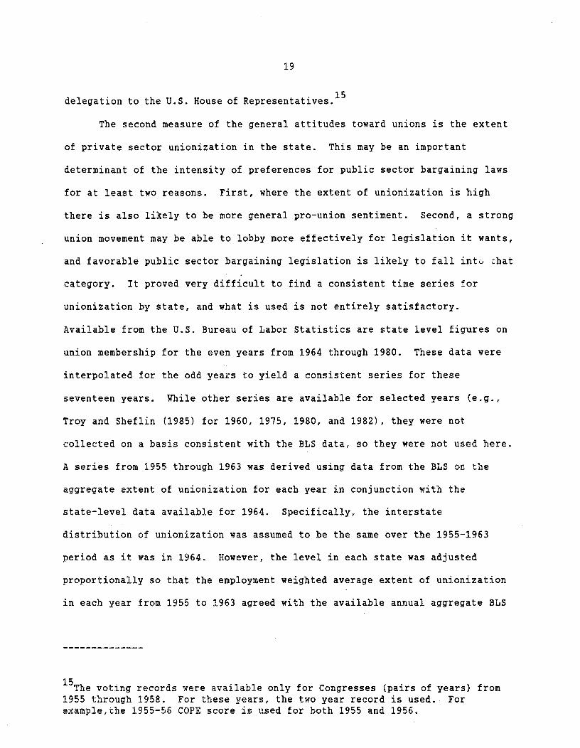
The second measure of the general attitudes toward unions is the extent

of private sector unionization in the state. This may be an important

determinant of the intensity of preferences for public sector bargaining laws

for at least two reasons. First, where the extent of unionization is high

there is also likely to be more general pro-union sentiment. Second, a strong

union movement may be able to lobby more effectively for legislation it wants,

and favorable public sector bargaining legislation is likely to fall mt0 chat

category. It proved very difficult to find a consistent time series or

unionization by state, and what is used is not entirely satisfactory.

Available from the U.S. Bureau of Labor Statistics are state level figures on

union membership for the even years from 1964 through 1980. These data were

interpolated for the odd years to yield a consistent series for these

seventeen years. While other series are available for selected years (e.g.,

Troy and Sheflin (1985) for 1960, 1975, 1980, and 1982) , they were not

collected on a basis consistent with the BLS data, so they were not used here.

A series from 1955 through 1963 was derived using data from the BLS on the

aggregate extent of unionization for each year in conjunction with the

state—level data available for 1964. Specifically, the interstate

distribution of unionization was assumed to be the same over the 1955—1963

period as it was in 1964. However, the level in each state was adjusted

proportionally so that the employment weighted average extent of unionization

in each year from 1955 to 1963 agreed with the available annual aggregate BLS

15The voting records were available only for Congresses (pairs of years) from

1955 through 1958. For these years, the two year record is used. Forexample,the 1955—56 COPE score is used for both 1955 and 1956.

20

data. In other words, the 1964 state level data were used to fix the relative

unionization across states and the annual aggregate data were used to fix the

overall level of unionization. An analogous technique was used to derive

state level data for 1981—1984 using the 1980 relative unionization across

states and the annual aggregate BLS data.

The third measure of general attitudes toward unionization is a dummy

variable for states that are in the south. While it is well known that

unionization is lower in the south, there may be negative attitudes regarding

unions in the south that go beyond the lower extent of unionization. Evidence

is provided by Farber (1983, 1984) not only that workers in the south are

less interested in unionization than workers outside that region but also that

workers in the south who do want union jobs are less likely to be able to

find union jobs, perhaps for institutional reasons. He also finds that the

existence of right—to—work laws in many states in the south does not account

for this inability to find union jobs.

Three other measures that may be related to the intensity of preferences

for public sector unionization are also used. The first is the level of per

capita income in the state. Where per capita income is higher, it may be that

the citizenry demands more public services and values them more highly so that

public employees have more power that they can use to create an environment

favorable to unionization. Alternatively, the citizenry may view unionization

of public employees as a normal good so they create an environment favorable

to public sector unionization where incomes are high. The precise measure

used is real per capita income in 1967 dollars.

The second measure is designed to reflect the size of the government

sector. Where the government sector is larger, public sector employees are

likely to have more power and influence that they can use to promote

legislation favorable to public sector collective bargaining. The measure

21

used is the ratio of state and local government expenditures to income in the

state.

The final measure used is a time trend measured by the year (55—SO).

This measure is included to capture a secular increase in preferences for

public sector unionization. It reflects the hypothesis that the reason for

the implementation of many favorable public sector bargaining laws over this

period is simply a secular improvement in public attitudes regarding public

sector unionization and/or a secular increase in public employees' demands

for unionization.

The value of no explicit policy toward public sector bargaining depends

heavily on the underlying attitudes toward unionization in the state. For

example, attempts to unionize by public sector employees in a state very

hostile to collective bargaining are likely to meet with strong resistance

from employers, the populace, and possibly the courts. The result is a de

facto unfavorable public policy toward unionization. Similarly, attempts to

unionize by public sector employees in a state that is sympathetic to

collective bargaining are likely to meet with less resistance (and perhaps

implicit acceptance) from employers, the populace, and the courts. The result

is a de facto favorable public policy toward unionization. On this basis, the

same set of variables argued to determine the intensity of preference for

unionization are argued to determine the value of no policy.

VII. Results

The econometric specification derived in section IV was estimated by

maximum likelihood using the data from the NBER public sector bargaining law

22

data set described in section ii.16 The first panel of table 6 contains the

definitions of three vectors of explanatory variables that are used in the

estimation: 1) Z contains only a constant, 2) Z2contains the full set of

five explanatory variables described in section V for the cost of policy

change, and 3) Z3 contains the full set of seven explanatory variables

described in section VI for the intensity of preference and the value of no

policy.

The second panel of table six contains a summary of eight specifications

(various combinations of the Z's) used to estimate the model for each of the

three employee groups. The first specification is a baseline with only

constants in the three vectors (cost of policy change, intensity of

preference, value of no policy). This model has a total of six parameters:

three constants and three breakpoints. The second specification is fully

unconstrained in that the full set of variables for each of the three vectors

is included: 1) for the cost of policy change vector, 2) for the

intensity of preference vector, and 3) Z3 for the value of no policy vector.

This specification has a total of twenty—two parameters. The next three

specifications in turn have only a constant in one of the three vectors. The

final three specifications have only a constant in two of the three vectors.

The last panel in table 6 contains maximized log—likelihood values for

each of the eight specifications for each of the three employee groups. These

are used to evaluate the various specifications.

Before comparing the different specifications, it is useful to examine

the estimates of the unconstrained model (specification #2).

16The numerical optimization was carried out using the algorithm described byBerndt, Hall, Hall, and Hausman (1974).

TABLE 6

Model Summary

Vector Definitions'

zi z2 z2

Constant Constant Constant

Legday COPENenact UnionUnified SouthYear Inc/Pop

Govexp/Inc

°See Table 5 for variable definitions.

Model Specifications

1 2 3 4 5 6 7 8

Cost of Policy Change Z2 Z2 Z2 Z1 Z1

Intensity of PreferenceZ1 Z3 Z3 Z1 Z3 Z.3 Z1

Value of no PolicyZ1 Z Z3

# of parameters 6 22 16 16 18 10 12 12

Log-Likelihood Values

Emp1oyGroup 1 2 3 4 5 6 7 8

State Employees —280.0 —250.4 —254.7 —265.8 —252.2 —276.6 —256.0 —266.8

PoU.ce —272.7 —242.9 —247.1 —258.8 —243.6 —270.4 —247.4 —259.5

Teachers —316.3 —270.0 —281.5 —294.2 —273.5 —311.0 —284.1 —296.7

23

The results are not encouraging with regard to the determinants of the

cost of policy change. For state employees, (table 7a), none of the variables

seem to affect the cost of policy change significantly in the hypothesized

direction. Only the number of bill enacted (nenact) has a coefficient that is

significantly different from zero at conventional levels, and that has the

wrong sign. The results are no better for police or teachers (tables 7b and

7c respectively). Again, none of the variables hypothesized to affect the

cost of policy change have coefficients that are significantly different from

zero in the appropriate direction. In addition, the hypothesis that all of

the coefficients in the cost of policy change vector except the constant term

are zero cannot be rejected using a likelihood—ratio test at any reasonable

level of significance for any of the three employee groups. These tests are

based on comparisons of the log—likelihoods for specification 5 with those for

specification 2. The conclusion is that the set of variables used to

determine the cost of policy change is not appropriate for any of the three

employee groups.

The intensity of preference function performs better. For state

employees, the COPE scores are significantly positively related to preference

while in the south preferences are significantly lower. It is interesting

that after controlling for the COPE scores and for South, the extent of

private sector unionization is not a significant determinant of preference for

public sector collective bargaining for state employees, and it has the wrong

sign. The value of per capita income is marginally significantly positively

related to preference, but the size of the government sector, as proxied by

the ratio of state and local government expenditures to total income, is not

significantly related. There is no significant time trend in preferences.

The estimates of the determinants of intensity are similar but somewhat less

well determined for police and teachers. In all three cases the hypothesis

24

that all of the coefficients in the intensity of preference vector except the

constant term are zero can be rejected using a likelihood—ratio test at any

reasonable level of significance. These tests are based on comparisons of the

log—likelihoods for specification 4 with those for specification 2. The

conclusion is that the set of variables used to determine the intensity of

preference has significant explanatory power for all three groups.

The value of no policy function is not very well determined for any of

the three employee groups. None of the estimated coefficients are

significantly different from zero for any of the groups. For both state

employees and police, the hypothesis that all of the coefficients in the value

of no policy vector except the constant term are zero cannot be rejected using

a likelihood—ratio test at any reasonable level of significance. However, for

teachers this hypothesis can be rejected, suggesting that the value of no

policy does vary systematically in the measured dimensions for teachers.

These tests are based on comparisons of the log—likelihoods for specification

3 with those for specification 2. The conclusion is that the set of variables

used to determine the value of no policy has significant explanatory power

only for teachers.

Overall, the estimates in tables 7a through 7c are not terribly

encouraging with regard to the model. It is true that for all three employee

groups the hypothesis that all parameters except the three constant terms and

the three breakpoints are zero (specification 1) can be rejected against

specification 2 at conventional levels of significance using a likelihood

ratio test. However, as is clear from the above discussion, only the

coefficients of the variables determining the intensity of preference are

consistently significantly different from zero as a group. In no case are the

parameters of the cost of policy change function significantly different from

zero, and only for teachers are the parameters of the value of no policy

TABLE7a

Narkov Model of Public Sector1Bargaining LawsState Employees

Cost of Policy Intensity of Value of

Change Preference No Policy

Constant 3.60 Constant 3.60 7.54

(2.28) (4.09) (4.31)

Legday .000298 COPE 2.50 —1.55(.00137) (1.16) (1.25)

Nenact .000695 Union —4.95 6.89(.000244) (3.80) (4.19)

Unified —.324 South —1.32 .731

(.237) (.661) (.749)

Year .00221 Inc/Pop .945 —.758(.0343) (.658) (.741)

Govexp/Inc .922 2.05

(3.93) (5.88)

Year —.0429 .0911

(.0598) (.0665)

Summary Statistics Breakints

LLF = —250.4 2.00

(.487)

n = 1490.K2

2.71(.393)

Statisticb/ = 59.2

K33.20

(.471)

a!See Table 5 for defianitions and summary statistics of variables. Thespecification used is #2 in table 6. The numbers in parentheses areasymptotic standard errors.

The statistic is the likelihood ratio test statistic of a constrainedmodel with constants only. (6 parameters)

TABLE 7b

Markov Model of Public Stor Bargaining LawsPolice

Cost of Policy Intensity of Value of

Change Preference No Policy

Constant 2.87 Constant 2.69 —5.82(1.37) (7.87) (.841)

Legday .000686 COPE 2.08 —.889(.00143) (1.63) (1.71)

Nenact .000112 Union —3.36 3.78(.000254) (5.36) (5.64)

Unified .00581 South —1.36 1.09(.00232) (.779) (.829)

Year .00681 Inc/Pop 1.01 —.541(.0204) (.921) (.949)

Govexp/Inc 1.17 .194

(5.15) (6.24)

Year —.0432 .0705

(.115) (.124)

Summary Statistics BreakpjLLF = —242.9

K11.35

(.502)

n = 1490.K2

2.53

(.361)

Statistic = 59.2K3

2.77

(.369)

a/See Table 5 for definitions and summary statistics of variables. Thespecification used is 12 in table 6. The numbers in parentheses areasymptotic standard errors.

The statistic is the likelihood ratio test statistic of a constrainedmodel with constants only. (6 parameters)

TABLE 7c

Markov Model of Public Sector,Bargaining LawsTeachers a

Cost of Policy Intensity of Value ofChange Preference No Policy

Constant 3.16 Constant 1.47 —5.92(1.47) (5.08) (5.39)

Legday .00252 COPE 1.76 —.846(.00150) (1.29) (1.38)

Nenact .0000210 Union —1.29 1.79(.000292) (3.94) (4.28)

Unified —.0432 South —1.89 1.85(.194) (.965) (1.02)

Year —.00158 Inc/Pop .727 —.0958(.0220) (.645) (.690)

Govexp/Inc 1.99 —1.18(4.76) (6.24)

Year —.0174 .0640(.0805) (.0868)

Summary Statistics

LL1F = —269.9 1.09

(.44)

n = 1490.K2

2.60

(.288)

Statisticb/ = 928

K32.81

(.307)

a/See Table 5 for definitions and summary statistics of variables. Thespecification used is #2 in table 6. The numbers in parentheses areasymptotic standard errors.

b/The statistic is the likelihood ratio test statistic of a constrainedmodel with constants only. (6 parameters)

25

function significantly different from zero.

It may be that the estimation of three vectors of parameters for each

group is putting an excessive burden on the data. Using the likelihood values

in table 6 as a guide, more parsimonious specifications for each of employee

groups can be derived. For state employees and police a reasonable

specification has only constants in the cost of policy change and value of no

policy vectors but with the full set of parameters in the intensity of

preference vector. This is specification 7, and it is nested in

specifications 2, 3, and 5. Specification 7 cannot be rejected at

conventional levels against any of these three alternatives for either state

employees or police. For teachers a reasonable specification has only a

constant in the cost of policy change vector but with the full set of

parameters in the cost of policy change and the value of no policy vectors.

This is specification 5, and it is nested in specification 2. As noted above,

specification 5 cannot be rejected against specification 2 at conventional

levels for teachers. On this basis the discussion of results proceeds using

as preferred specifications 7 for state employees and police and 5 for

teachers.

Tables 8a and 8b contain estimates of specification 7 for state

employees and police respectively. It is clear that the restrictions embodied

in these specifications improve the precision of the parameter estimates

considerably. For state employees the estimates suggest that intensity of

preferences are significantly positively related to the COPE score and

negatively related to being in the southern region. In addition, intensity of

preferences is marginally significantly positively related to per capita

income and per capita government expenditures. The results in table 8b are

similar for police. Intensity of preferences are significantly positively

related to the COPE score and marginally significantly negatively related to

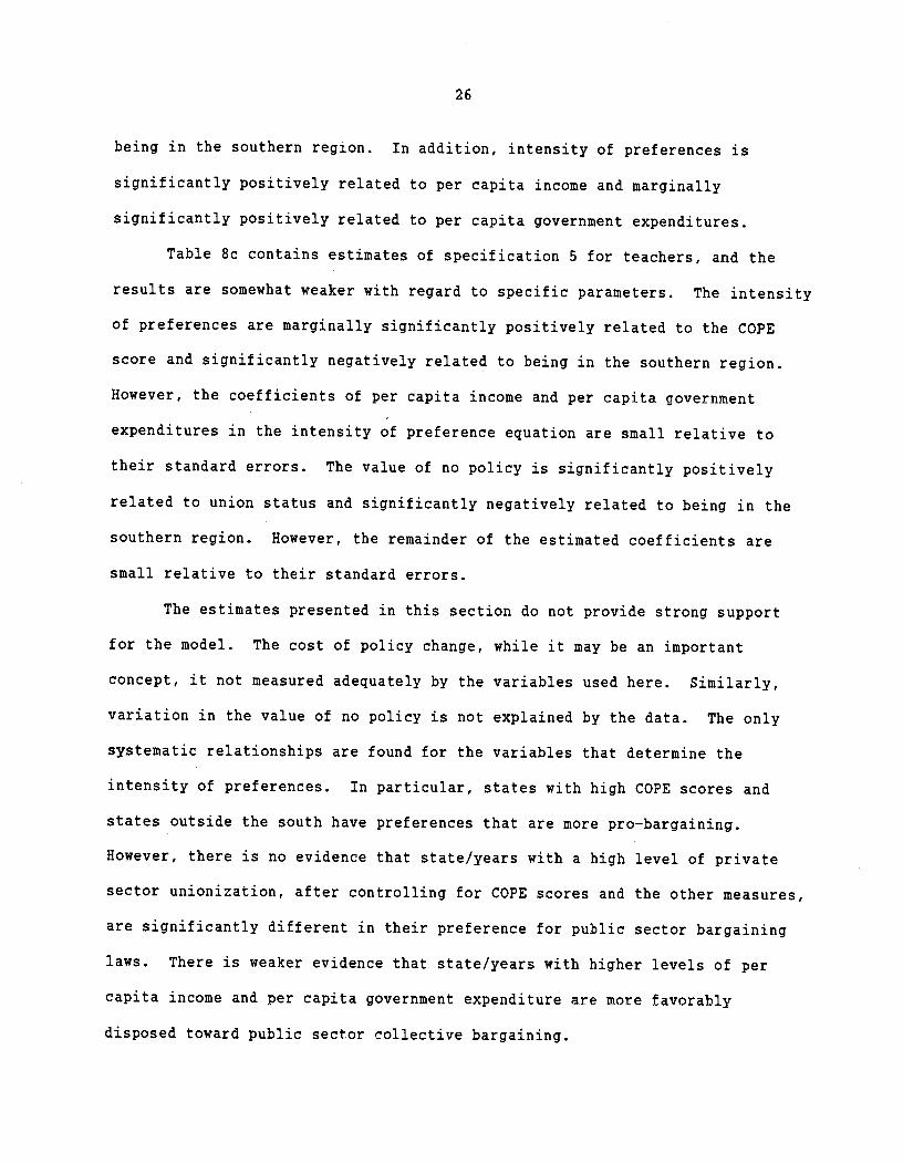
26

being in the southern region. In addition, intensity of preferences is

significantly positively related to per capita income and marginally

significantly positively related to per capita government expenditures.

Table 8c contains estimates of specification 5 for teachers, and the

results are somewhat weaker with regard to specific parameters. The intensity

of preferences are marginally significantly positively related to the COPE

score and significantly negatively related to being in the southern region.

However, the coefficients of per capita income and per capita government

expenditures in the intensity of preference equation are small relative to

their standard errors. The value of no policy is significantly positively

related to union status and significantly negatively related to being in the

southern region. However, the remainder of the estimated coefficients are

small relative to their standard errors.

The estimates presented in this section do not provide strong support

for the model. The cost of policy change, while it may be an important

concept, it not measured adequately by the variables used here. Similarly,

variation in the value of no policy is not explained by the data. The only

systematic relationships are found for the variables that determine the

intensity of preferences. In particular, states with high COPE scores and

states outside the south have preferences that are more pro—bargaining.

However, there is no evidence that state/years with a high level of private

sector unionization, after controlling for COPE scores and the other measures,

are significantly different in their preference for public sector bargaining

laws. There is weaker evidence that state/years with higher levels of per

capita income and per capita government expenditure are more favorably

disposed toward public sector collective bargaining.

TABLE 8a

Markov Model of Public Secto Bargaining LawsState Employeesa

Cost of Policy Intensity of Value of

Change Preference No Policy

Constant 3.41 Constant —.178 —1.95(.186) (1.69) (.351)

Legday COPE 1.18(.459)

Nenact Union .300

(1.31)

Unified South —.821

(.313)

Year Inc/Pop .359

(.248)

Govexp/ Inc 3.95

(2.64)

Year .0116

(.0307)

Summary Statistics ]oinLLF = —256.0

K11.68

(.460)

n = 1490.K2

2.40

(.322)

Statisticb/ = —48.0

1(32.90(.354)

a!See Table 5 for definitions and summary statistics of variables. Thespecification used is #7 in table 6. The numbers in parentheses areasymptotic standard errors.

The 2 statistic is the likelihood ratio test statistic of a constrainedmodel with constants only. (6 parameters)

TABLE 8b

Markov Model of Public Sect?r Bargaining LawsPolicea

Cost of Policy Intensity of Value ofChange Preference No Policy

Constant 3.36 Constant —.274 —1.69(.163) (1.70) (.303)

Legday COPE 1.31

(.448)

Nenact Union -.279(1.43)

Unified South —.497(.260)

Year Inc/Pop .604

(.256)

Govexp/Inc 3.93

(2.55)

Year — .00104(.0308)

Summary Statistics Breakpoints

LLF = —247.4K1

1.31

(.356)

n = 1490.K2

2.41

(.270)

x2 Statistic b/ = 50.61(3

2.63

(.267)

a!See Table 5 for definitions and summary statistics of variables. Thespecification used is #7 in table 6. The numbers in parentheses areasymptotic standard errors.

bfThe statistic is the likelihood ratio test statistic of a constrainedmodel with constants only. (6 parameters)

TABLE 8c

Markov Model of Public Secto,Bargaining LawsTeachers

Cost of Policy Intensity of Value of

Change Preference No Policy

Constant 3.23 Constant 1.60 —6.02(.151) (5.00) (5.31)

Legday COPE 1.67 —.751(1.29) (1.38)

Nenact Union —1.62 1.94(3.62) (.396)

Unified South —1.78 1.72

(.778) (.805)

Year Inc/Pop .630 —.0404(.610) (.668)

Govexp/Inc 3.19 —.894(4.79) (6.22)

Year —.0192 —.0623(.0773) (.0849)

Summary Statistics Breakpoints

LLF = —273.5K1

1.01

(.429)

n = 1490.K2

2.51(.240)

Statisticb/ = 85.6

K32.73(.264)

a!See Table 5 for definitions and summary statistics of variables.Thespecification used is #5 in table 6. The numbers in parentheses areasymptotic standard errors.

b/The statistic is the likelihood ratio test statistic of a constrainedmodel with constants only. (6 parameters)

27

VIII. How Well Does the Model Fit the Data?

At this point, it is important to ask how well the model fits the data.

While there is no consensus on an appropriate test of goodness—of—fit in a

model such as this, two related concepts are used. The first asks how well

the model can mimic the aggregate distribution of laws by category at five

year intervals. The second asks how well the model can differentiate the

states that have a given category of law from those that do not at five year

intervals.

The parameter estimates for any given specification can be used to

compute a predicted Markov transition matrix for any state i in any year t

using the probabilities defined in the appendix. Denote this one—period

transition matrix by M. whose jkth element is the predicted probability that

state i with law category j in year t—l will have law category k in year t.

On this basis the estimated transition matrix for state i over a n year period

from 1955 to 1955+n is55+n

(VIII.1) C. = II M.in itt =55

where II represents the matrix product. The average n—period transition matrix

over in states is

(VIII.2) =. C.

where > represents the matrix sum. The jkth element of this matrix represents

the average predicted probability that a state with category j law in 1954

will have category k law in year 1955+n.

The average transition matrix was computed for n=4,9,14.19,24,29

(corresponding to the years 1959, 1964, 1969, 1974, 1979, and 1984) for each

of the three employee groups. The preferred specifications were used for each

of the employee groups. These are based on the estimates in tables 8a, 8b and

8c for state employees, police, and teachers respectively. First order

28

approximations to the standard errors of the elements of these matrices were

17computed using the delta method

The first row of the transition matrix, , contains the averagen

probabilities that a state will have a law in each of the categories in year

1955+n conditional having no law in 1954. Since fewer than a handful of

states had any explicit policy regarding public sector collective bargaining

in 1954, it is appropriate to focus on this row of the matrix. If the model

fits the data well it ought to be true that at each of thefive year intervals

these transition probabilities ought to closely reflect the actual

distribution of laws at that point in time. The underlying conceptual

experiment is to assume that there were no laws in 1954 in any state and to

start the process of evolution of laws according to the estimated Markov

process. The interesting questions regard 1) the extent to which the

estimated Markov process can explain the movements over time in the fraction

of states with a law in a given category and 2) the extent to which by 1984

the cross—sectional distribution implied by the Markov process is similar to

the actual distribution. The average estimated transition probabilities along

with their asymptotic standard errors as well as the actual distribution of

laws for the six selected years are contained in tables 9a, 9b, and 9c for the

three employee groups respectively. The estimated probabilities sum to one by

now.

It is clear from the actual distribution of laws for state employees in

table 9a that most of the action in the enactment of laws was in the period

17The standard error of an element of the transition matrix is computed as thesquare—root of g'Vg where g is the gradient vector of the particular elementof the matrix with respect to the parameter vector and V is the estimatedasymptotic covariance matrix of the estimated parameters. The gradient vectorwere computed numerically.

29

from 1964 through 1979. This is indicated by the sharp rate of decline over

this period in the proportion of states with no law. The predicted proportion

with no law declined steadily from 1959 to 1984, but the model was not able to

fully capture the steeper decline between 1964 and 1979. The model

consistently overpredicted the fraction of states with category 1 laws

(prohibiting bargaining) after 1964. Roughly speaking, the model predicted

that this fraction remained constant at approximately 7.5 percent after 1964

while the actual distribution stabilized at approximately 15 percent after

1974. At the other extreme, the model did a slightly better job capturing the

emergence of category 4 laws (requiring bargaining). The observed fraction of

states with this type of law increased dramatically from 0 percent in 1964 to

46 percent by 1979. The model did not predict quite so rapid an increase, but

the predicted probabilities of category 4 laws did increase more rapidly over

the 1964 to 1979 period than either earlier or later. The cross—sectional

1984 distribution differs somewhat from the actual distribution in predicting

too high a fraction with no law and too low a fraction with a category 1 law.

Examination of the actual and predicted distribution of laws for police

in table 9b yields similar conclusions to those for state employees though the

model does seem to fit a somewhat better. The timing of the enactment of laws

governing collective bargaining for police was concentrated between 1964 and

1979, and the model was not able to pick this up as well as it might have.

The model did a better job fitting the fairly constant low probability of

having a category 1 law. The model was also able to capture a large share of

the rapid increase in the introduction of category 4 laws between 1964 and

1979. The predicted cross—sectional distribution for 1984 is quite close to

the actual 1984 distribution.

Table 9c contains the actual and predicted distributions for laws

governing teachers. The overall pattern of movement of the actual

30

distribution of laws over time is quite similar to the two other groups. The

model fits the data relatively well with the exception (common to the other

two groups) that the rapid decline between 1964 and 1979 in the fraction with

no law is not fully captured by the model. However the relative stability in

the fraction with a category 1 law, the rapid increase in the fraction with a

category 4 law, and the 1984 cross—sectional distribution are all captured

quite closely.

Overall, the model seems to do a reasonable job in explaining the

aggregate distribution of laws at given five year intervals. A more difficult

task for the model is to predict which states have laws of a given type at any

point in time. One way to examine the ability of the model to predict which

states will have laws of a given type is to examine the average predicted

probabilities that a state will have have a law of a given type in a given

year where the average is taken only over states with a law of that type. For

example, it is useful to examine the average predicted probability for states

that have a category 1 law in a given year that those states will, in fact,

have a category 1 law.

The average n—period transition matrix required for this exercise is

defined similarly to that in equation VIII.2 as

(VIII.3) C =. E C.nk in innk iSnk

where Sk is the set of states with category k law in year 1955+n,k is the

number of elements in S , and C. is defined in equation VIII.1. Thenk in

conceptual experiment is the same as that underlying tables 9a—9c in the sense

that it is assumed that no states have laws in 1954 and that the process of

evolution of laws is governed by the estimated Markov process. If the model

predicted perfectly then the estimated probability that a state with category

j law in fact has a category j law would equal one. The estimated probability

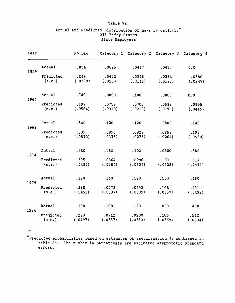
Table 9a:

Actual and Predicted Distribution of Laws by CategoryAll Fifty StatesState Employees

Year No Law Category 1 Category 2 Category 3 Category 4

Actual .854 .0625 .0417 .0417 0.01959

Predicted .849 .0472 .0376 .0284 .0380(s.e.) (.0379) (.0200) (.0141) (.0123) (.0247)

Actual .740 .0800 .100 .0800 0.01964

Predicted .697 .0756 .0703 .0582 .0995(s.e.) (.0564) (.0318) (.0218) (.0198) (.0445)

Actual .540 .120 .120 .0800 .1401969

Predicted .539 .0896 .0929 .0858 .193(s.e.) (.0572) (.0375) (.0273) (.0261) (.0530)

Actual .280 .160 .100 .0800 .3801974

Predicted .395 .0864 .0996 .103 .317(s.e.) (.0484) (.0364) (.0304) (.0322) (.0494)

Actual .180 .140 .120 .100 .4601979

Predicted .288 .0778 .0953 .108 .431(s.e.) (.0451) (.0337) (.0309) (.0357) (.0492)

Actual .160 .160 .120 .080 .4801984

Predicted .220 .0712 .0900 .106 .512(s.e.) (.0497) (.0337) (.0312) (.0369) (.0634)

°Predicted probabilities based on estimates of specification #7 contained intable 8a. The number in parentheses are estimated asympototic standarderrors.

Table 9b:Actual and Predicted Distribution of Laws by Category°

All Fifty StatesPolice

Year No Law Category 1 Category 2 Category 3 Category 4

Actual .896 .0625 .0208 .0208 0.01959

Predicted .848 .0365 .0523 .0138 .0495(s.e.) (.0349) (.0180) (.0161) (.00737) (.0269)

Actual .740 .0600 .140 .0400 .02001964

Predicted .689 .0581 .0994 .0279 .125(s.e.) (.0510) (.0270) (.0247) (.0131) (.0458)

Actual .480 .0800 .200 .0400 .2001969

Predicted .519 .0658 .135 .0410 .238(s.e.) (.0511) (.0292) (.0321) (.0186) (.0530)

Actual .260 .0400 .160 .0400 .5001974

Predicted .362 .0576 .151 .0487 .381(s.e.) (.0434) (.0249) (.0379) (.0227) (.0501)

Actual .180 .0600 .180 .0400 .5401979

Predicted .248 .0465 .150 .0504 .505(s.e.) (.0412) (.0207) (.0407) (.0244) (.0533)

Actual .160 .0800 .180 .0400 .5401984

Predicted .180 .0397 .146 .0496 .585(s.e.) (.0453) (.0204) (.0425) (.0247) (.0690)

°Predicted probabilities based on estimates of specification #7 contained intable 8b. The number in parentheses are estimated asympototic standarderrors.

Table 9c:Actual and Predicted Distribution of Laws by Category

All Fifty StatesTeachers

Year No Law Category 1 Category 2 Category 3 Category 4

Actual .896 .0625 .0208 .0208 0.01959

Predicted .858 .0367 .0608 .00909 .0375(s.e.) (.0331) (.0184) (.0203) (.00479) (.0166)

Actual .740 .0600 .120 .0600 .02001964

Predicted .685 .0483 .130 .0227 .115(s.e.) (.0538) (.0231) (.0341) (.0101) (.0381)

Actual .440 .0600 .240 .0800 .1801969

Predicted .460 .0544 .188 .0381 .259(s.e.) (.0536) (.0219) (.0452) (.0169) (.0535)

Actual .160 .0400 .200 .0400 .5001974

Predicted .237 .0592 .213 .0474 .443(s.e.) (.0421) (.0201) (.0485) (.0227) (.0561)

Actual .0600 .0800 .240 .0200 .6001979

Predicted .0962 .0697 .209 .0470 .578(s.e.) (.0337) (.0267) (.0466) (.0242) (.0590)

Actual .0600 .0800 .240 .0200 .6001984

Predicted .0334 .0836 .202 .0426 639(s.e.) (.0237) (.0478) (.0484) (.0233) (.0813)

apdid probabilities based on estimates of specification #5 contained intable 8c. The number in parentheses are estimated asympototic standarderrors.

31

that the state has a law in any other category would equal zero. While there

is no chance that the model will do this well, the interesting question that

can be answered by this analysis is whether the estimated probabilities for a

state with a given category law are skewed toward the type of law that the

state, in fact, has.

Tables lOa, lOb, and lOc contain estimated transition probabilities and

standard errors for the three employee groups respectively. The calculations

are presented for the three selected years 1964, 1974, and 1984 (corresponding

to n=9l9,29). Three subsets of states in each year are used: 1) states with

no law, 2) states with category 1 laws, and 3) states with category 4 laws.

The estimated probabilities sum to one by now.

The estimates in table lOa, for laws governing state employees, are not

very encouraging. For states with no law, the estimated probability that the

state, in fact, has no law is substantially different from one even in 1964

and declines dramatically by 1984. Even worse, the estimated probabilities

are virtually indistinguishable from those contained in table 9a computed

using all fifty states. For states with type 1 laws, the model does a bit

better. The estimated probabilities are still dramatically smaller than one,

but they are substantially larger than those contained in table 9a computed

using all fifty states. For states with type 4 laws, the estimated

probabilities are again dramatically smaller than one, and they are again

larger than those contained in table 9a computed using all fifty states.

The results contained in table lOb for laws governing police are

qualitatively identical to those for laws governing state employees. The

model does a poor job distinguishing states that have no law, but it does a

somewhat better job identifying states that have anti—bargaining or

pro—bargaining laws. The estimates contained in table lOc suggest that the

model performs even more poorly for laws governing teachers. The model can

32

neither distinguish states that have no law, nor distinguish states that have

anti—bargaining or pro—bargaining laws. Basically, the probabilities

presented in table lOc computed using only the states with specific categories

of laws are not very different at all from the probabilities presented in

table 9c computed using all fifty states.

IX. Conclusions

The character of both the parameter estimates presented in section VII

and. the estimated transition probabilities presented in section VIII lead to

the inescapable conclusion that the model, as estimated, does not adequately

explain the evolution of public sector bargaining laws. However, the model

was successful in some dimensions. A number of variables (COPE scores, South,

per capita income, per capita government expenditures) were found to be

systematically related to the intensity of preferences for public sector

collective bargaining. In addition, the model seems to perform adequately in

explaining the aggregate distribution of bargaining laws at a point in time.

It did particularly well explaining the 1984 cross—section.

On the negative side, virtually nothing was found that was

systematically related to the cost of policy change. Whether this is due to

having chosen the wrong set of variables to explain these costs or this is due

to the concept itself being misguided is difficult to know. However, one

piece of evidence in support of the concept is that when the cost of policy

change is estimated as a constant alone plus a stochastic term, the constant

term is estimated to be significantly different from zero. Were there no

rigidity in policy determination, the estimate of this constant would be

insignificantly different from zero.

Another important negative for the model is its failure to be able to

predict which states (as opposed to how many) had laws of a given category in

34

REFERENCES

Berndt, E. K., B. H. Hall, R. E. Hall, and 3. A. Hausman, "Estimation andInference in Nonlinear Structural Models," Annals of Economic and SocialMeasurement 3/4, 1974, pp. 653—665.

Dalton, Amy. "A Theory of the Organization of State and Local GovernmentEmployees", Journal of Labor Research, Spring 1982, 3(2), Pp. 163—77.

Faber, Charles F. arid Donald L. Martin Jr. "Two Factors Affecting Enactment ofCollective Bargaining Legislation in Public Education", Journal ofCollective Negptiations, 1979, 8(2), pp. 151—59.

Farber, Henry S.. "The Determinationof the Union Status of Workers,"Econometrica, September 1983: pp. 1417—1437.

Farber, Henry S. "Right to Work Laws and the Extent of Unionization," Journalof Labor Economics, July 1984: pp. 319—352.

Freeman, Richard B. "Unionism Comes to the Public Sector", Journal of Economic

Literature, Vol. XXIV, March 1986, pp. 41-86.

Freeman, Richard B. and James L. Medoff. "New Estimates of Private SectorUnionism in the United States", Industrial and Labor Relations Review,January 1979, 32(2), pp. 143—174.

Ichniowski, Casey. "Bargaining Laws and Police Union Growth: A ProportionalHazards Approach with Time—Varying Treatments", forthcoming in RichardB. Freeman and Casey Ichniowski eds., WhenUnionize, (University of Chicago Press), 1988.

Kochan, Thomas A. "Correlates of State Public Employee Bargaining Laws",Industrial Relations, October 1973, 12(3), pp. 322—37.

Kokkelenberg, Edward C. and Donna R. Sockell, Industrial and Labor Relations

Review, July 1985, 38(4), pp. 497—543.

Lauer, Harrison S. "The Effect of Collective Bargaining in Municipal PoliceForces on Wages, Salaries, and Fringe Benefits", Undergraduate Thesisfor Department of Economics, Harvard College, March 1979.

Moore, William J. "Factors Affecting Growth in Public and Private SectorUnions", Journal of Collective Negotiations, 1977, 6(1), pp. 37—43.

Reid, Joseph D., Jr. and N. Kurth. "The Importance of Union Security to theGrowth of Unionism", October 1983.

Saltzman, Gregory N. "Bargaining Laws as a Cause and Consequence of the Growthof Teacher Unionism", Industrial. and Labor Relations Review, April 1985,38(3), pp. 335—351.

Troy, Leo and Neil Sheflin. Union Sourcebook: Nembershi Finances, StructurDirectory, IRDIS, West Orange, New Jersey, 1985.

Valletta, R. G. and R. B. Freeman. "Presentation of NBER State Public SectorCollective Bargaining Law Data Set", NBER mimeo, June 1986

APP-i

APPENDIX

Specification of Transition Probabilities

In this appendix, the twenty—five elements of the Narkov transition

matrix are defined. The four elements associated with movement from an

existing policy to no policy are assumed to equal zero by definition. These

are

(A.i) P = Pr(J =OJJ =m) = 0 V'm=i,2,3,4.mO t—1

The remaining twenty—one elements are described in the remainder of this

appendix as functions of the latent variables defined in section IV.

Row 1: No preexisting policy (J1=0).

In this case a state will remain without a policy if the absolute value

of the deviation of the intensity of preferences from the value of no policy

is less than the cost of change. In terms of the latent variables, the

probability of this event is

(A.2) Pr(J,=0lJ1=O) = Pr(—Y1 < Y2—Y3 < Y1)

=Pr(Y1+Y2—Y3>0, Y,—Y3—Y1 <0)

=Pr(—1—c2<X1I31+X2I32—X3f3, c2—1<X1/31—X3/33—X/3)

=Pr(—e1—c,<X1/31—X3/33+X2/32)pr(—E<X/3—X/—X/3)This bivariate normal probability reduces to the product of two univariate

normal CDF's because the correlation of and E— is zero under the

assumption of equal variances for and

The detail of presentation of Pr(J=O!=0) is to illustrate how the

elements of the specification are tied together. This level of detail will

not be continued for all of the probabilities in this section.

When a state with no policy enacts a law in the most unfavorable

category (#1) it is known that the absolute value of the deviation of the

intensity of preferences from the value of no policy is greater than the cost

of change and that intensity of preferences are lower than the bottom

APP-2

threshold (K1). The probability of this event is

(A.3) Pr(J=lIJ1=O) =Pr({Y2—Y3<—Y1 orY2—Y3>Y1], Y2<K1)

which can be expressed as suns of bivariate normal CDF's that are easily

approximated numerically.

When a state with no policy enacts a law in an intermediate category m

(#2 or #3) it is known that the absolute value of the deviation of the

intensity of preferences from the value of no policy is greater than the cost

of change and that intensity of preferences are bounded by the thresholds K1

and K. The probability of this event is

(A.4) Pr(J=mIJ1=O) =Pr(fY2—Y3<—Y1 2Y2_Y3>YiLKmj<Y2<Km)

for m=2,3. Once again, this can be expressed in terms of sums of bivariate

normal CDF's.

Finally, when a state with no policy enacts a law in the highest

category (#4) it is known that the absolute value of the deviation of the

intensity of preferences from the value of no policy is greater than the cost

of change and that intensity of preferences are greater than the threshold K3.

The probability of this event is

(A.5) Pr(J=4J1=O) = Pr([Y2—Y3<—Y1 orY2-Y3>Y1], Y2>K3)

which again be expressed in terms of bivariate normal CDF's.

Taken together these probabilities completely specify the likelihood of

all possible events for the cases where there had existed no policy. It is

straightforward to demonstrate that these probabilities sum to one. The

parameters of this specification include /3 21 f3, and the three thresholds

K1, K2, and K3.

Row 2: A pre—existirig policy in the lowest gr (J=1),

The first possibility is that no change in the law was made. In this

case it is known that the intensity of preferences are not high enough to

APP—3

warrant a change. Specifically, it is known that the intensity of preferences

is less than the bottom threshold plus the cost of making a change. The

probability of this event is

(A.6) Pr(J=1 1=1) =Pr(Y2 <K1 +Y).

=Pr(E2—1<K1—X2/32+X1/31)

which is simply a univariate normal CDF.

While it was relatively rare (see table 4) for a state to change its

policy from one that prohibited bargaining to a more favorable category, it

did happen. If a state were to change its policy from one of prohibiting

bargaining to an intermediate category, in, it would be known that the

intensity of preference exceeded the lower threshold (K1) by more than the

cost of change and that the intensity of preference lay in the appropriate

interval (between K1 and K). The probability of this event is

(A.7) Pr(J=mJ1=l) =Pr(Y2)K1+Y1, K1<Y2<K)= Pr(Y -Y <-K ,K <Y <K

1 2 1 rn—I 2 rn

which can be expressed in terms of bivariate normal CDF's.

The final possibility for a state with a policy of prohibiting

bargaining is to enact a policy in the most favorable category (#4, requiring

bargaining). In this case, it would be known that the intensity of preference

exceeded the lower threshold (K1) by more than the cost of change and that the

intensity of preference also exceeded the highest threshold (K3). The

probability of this event is

(A.8) Pr(J=4J1=l) =Pr(Y2>K1+Y1, Y2>K3)

= Pr(Y1—Y2<—K ,Y2 > K3)

which can be expressed in terms of bivariate normal CDF's.

Equations A.6—A.8 define the probabilities of all possible events for

the case where there existed a policy in the lowest category. It is

straightforward to demonstrate that these probabilities sum to one. The

APP—4

parameters of these probabilities include /3 , 2' and the three thresholds K1

K2 , and K3. Note that these probabilities are not a function of /33. which

determines the value of no policy.

Row 3: Pre—existing policy in category 2 (J1=2).

The first possibility is that no change in the law was made. In this

case it is known that the intensity of preferences are not high enough or low

enough to warrant a change. More specifically, it is known that the intensity

of preferences is both greater than the lower threshold (K1) minus the cost of

making a change and less than K2 plus the cost of making a change. The

probability of this event is

(A.9) Pr(J=2IJ1=2) =Pr(K1—Y1 (Y2(K24-Y1).

which can be expressed as sums of bivariate normal CDF's.

If a state were to change its policy from category 2 to the lowest

category it would be known that the intensity of preferences was less

than the lower threshold by an amount at least as large as the cost of

change. The probability of this event is

(A.lO) Pr(J=llJ1=2) =Pr(Y2(K1—Y1).

which is simply a univariate normal CDF.

Movement from category 2 to category 3 occurs when the intensity of

preferences exceeds K2 by more than the cost of a policy change and

the intensity of preferences is in the interval from2K to3K. The

probabilityof this event is

(A.ll) Pr(J=3I1=2) =Pr(Y2>K2+Y1,K2Y2K3)

which again can be computed from sums of bivariate normal CDF's.

Finally, if a state were to change its policy from category 2 to the

highest category (#4, requiring bargaining) it would be known that the

intensity of preferences exceeded K7 by more than the cost of a policy change

APP—5

and that the intensity of preferences was greater than the highest threshold

(K3). The probability of this event is

(A.12) Pr(J.=4IJLl=2) =Pr(Y2>K2+Y,Y>K3).

which can be computed from sums of bivariate normal CDF's.

Equations A.9—A.12 define the probabilities of all possible events for

the case where there existed a category 2 policy. It is straightforward to

demonstrate that these probabilities sum to one. The parameters of these

probabilities include and the three thresholds K1 , K2, and K3.

Row 4: Pre—existing pplicy in category 3

The first possibility is that no change in the law was made. In this

case it is known that the intensity of preferences are not high enough or low

enough to warrant a change. More specifically, it is known that the intensity

of preferences is both greater than K2 minus the cost of making a change and

less than the upper threshold (K3) plus the cost of making a change. The

probability of this event is

(A.13) Pr(J.,=3J(,1=3) =Pr(K2—Y1(Y2<K3+Y1).

which can be expressed as sums of bivariate normal CDF's.

If a state were to change its policy from category 3 to the lowest

category it would be known that the intensity of preferences was less than K2

by an amount at least as large as the cost of change and the intensity of

preferences was less than the lowest threshold. The probability of this event

is

(A.14) Pr(J=lIJt1=3) = Pr(Y2<K2—Y1Y2<K1).

which can be expressed as sums of bivariate normal CDF's.

Movement from category 3 to category 2 occurs when the intensity of

preferences is less than K2 by an amount at least as large as the cost of

change and the intensity of preferences is greater than the lowest threshold.

APP —6

The probability of this event is

(A..15) Pr(J=2 = Pr(Y2<K2—Y11Y2'K1)

which again can be computed from sums of bivariate normal CDF's.

Finally, if a state were to change its policy from category 3 to the

highest category (#4, requiring bargaining) it would be known that the

intensity of preferences exceeded K3 by more than the cost of a policy change.

The probability of this event is

(A.16) Pr(J(=4IJl=3) =Pr(Y2>K3+Y1).

which is a univariate normal CDF.

Equations A.13—A.16 define the probabilities of all possible events for

the case where there existed a category 3 policy. It is straightforward to

demonstrate that these probabilities sum to one. The parameters of these

probabilities include and the three thresholds K1 , K2, and K3.

Row 5: Pre—existing Polici in the highest categry (3 =4).

Finally, consider the case where the state had a law requiring

bargaining (category #4). While it is conceptually possible for a state to

move to a less favorable policy (if intensity of preference becomes less than

the highest threshold (K3) by more than the cost of change), this was never

observed for the three employee groups over the 30 year period covered (see

table 4). Nonetheless, the probabilities of these events will be required

when the parameter estimates are used to compute predicted legal status at

various points in time.

In the case where there is no change in policy (all of the observed

cases), it is known that the intensity of preferences exceeds the highest

threshold minus the cost of a policy change. This probability is

(A.17) Pr(J=4J1=4) =Pr(Y2>K3—Y1)

which is a univariate normal CDF.

APP—7

If the policy were to change to the lowest category it would be known

that the intensity of preferences is less than the highest threshold minus the

cost of a policy change and that the intensity of preferences is less than the

lowest threshold. The probability of this event is

(A.18) Pr(J=1JJ1=4) =Pr(Y2K3—Y1 ,Y2<K1)

which can be evaluated as a bivariate normal CDF.

If the policy were to change to category 2 it would be known that the

intensity of preferences is less than the highest threshold minus the cost of

a policy change and that the intensity of preferences lies between K1 and K2

The probability of this event is

(A.19) Pr(J,=2IJ1=4) =Pr(Y7<K3—Y1,K1(Y2<K2)

which can be evaluated as sums of bivariate normal CDF's.

Finally, if the policy were to change to category 3 it would be known

that the intensity of preferences is less than the highest threshold minus the

cost of a policy change and that the intensity of preferences lies between K2

and K3 The probability of this event is

(A.20) Pr(J=3JiJ1=4) =Pr(Y2(K3—Y1 ,K2(Y2(K3)

which can be evaluated as sums of bivariate normal CDF's.

Equations A.17—A.20 define the probabilities of all possible events for

the case where there existed a category 4 policy. It is straightforward to

demonstrate that these probabilities sum to one. The parameters of these

probabilities include 2' and the three thresholds K1, K2, and K3.