NBER WORKING PAPER SERIES

THE TERM STRUCTURE OF THE RISK-RETURN TRADEOFF

John Y. CampbellLuis M. Viceira

Working Paper 11119http://www.nber.org/papers/w11119

NATIONAL BUREAU OF ECONOMIC RESEARCH1050 Massachusetts Avenue

Cambridge, MA 02138February 2005

This material is based upon work supported by the National Science Foundation under Grant No. 0214061to Campbell. Viceira acknowledges the financial support of the Division of Research of the Harvard BusinessSchool. The views expressed herein are those of the author(s) and do not necessarily reflect the views of theNational Bureau of Economic Research.

© 2005 by John Y. Campbell and Luis M. Viceira. All rights reserved. Short sections of text, not to exceedtwo paragraphs, may be quoted without explicit permission provided that full credit, including © notice, isgiven to the source.

The Term Structure of the Risk-Return TradeoffJohn Y. Campbell and Luis M. ViceiraNBER Working Paper No. 11119February 2005JEL No. G12

ABSTRACT

Recent research in empirical finance has documented that expected excess returns on bonds and

stocks, real interest rates, and risk shift over time in predictable ways. Furthermore, these shifts tend

to persist over long periods of time. In this paper we propose an empirical model that is able to

capture these complex dynamics, yet is simple to apply in practice, and we explore its implications

for asset allocation. Changes in investment opportunities can alter the risk-return tradeoff of bonds,

stocks, and cash across investment horizons, thus creating a ``term structure of the risk-return

tradeoff.'' We show how to extract this term structure from our parsimonious model of return

dynamics, and illustrate our approach using data from the U.S. stock and bond markets. We find that

asset return predictability has important effects on the variance and correlation structure of returns

on stocks, bonds and T-bills across investment horizons.

John Y. CampbellDepartment of EconomicsLittauer Center 213Cambridge, MA 02138and NBERjohn_campbell@harvard.edu

Luis M. ViceiraMorgan Hall 395Graduate School of Business AdministrationHarvard UniversityBoston, MA 02163and NBERlviceira@hbs.edu

1 Introduction

Recent research in empirical finance has documented that expected excess returns onbonds and stocks, real interest rates, and risk shift over time in predictable ways.Furthermore, these shifts tend to persist over long periods of time. Starting at leastwith the pioneering work of Samuelson (1969) and Merton (1969, 1971, 1973) onportfolio choice, financial economists have argued that asset return predictability canintroduce a wedge between the asset allocation strategies of short- and long-terminvestors.

One important implication of time variation in expected returns is that investors,particularly aggressive investors, may want to engage in market-timing (or tacticalasset allocation) strategies aimed at maximizing short-term return, based on the pre-dictions of their return forecasting model. However, there is considerable uncertaintyabout the degree of asset return predictability and this makes it hard to identify theoptimal market-timing strategy. A second, less obvious implication of asset returnpredictability is that risk–defined as the conditional variances and covariances perperiod of asset returns–may be significantly different across investment horizons,thus creating a “term structure of the risk-return tradeoff.” This tradeoff is the focusof this paper.

This paper examines the implications for risk across investment horizons of timevariation in investment opportunities. To this end we propose an empirical model thatis able to capture the complex dynamics of expected returns and risk, yet is simpleto apply in practice. Specifically, we model interest rates and returns as a vectorautoregressive model (VAR).2 We show how one can easily extract the term structureof risk using this parsimonious model of return dynamics, and illustrate our approachusing quarterly data from the U.S. stock, bond and T-bill markets for the postwarperiod. In our empirical application we use variables that have been identified asreturn predictors by past empirical research, such as the short-term interest rate, thedividend-price ratio, and the yield spread between long-term and short-term bonds.3

2This type of specification has been used in a similar context by Kandel and Stambaugh (1987),Campbell (1991), Hodrick (1992), Campbell and Viceira (1999), Barberis (2000), and Campbell,Chan and Viceira (2003) among others.

3See Fama and Schwert, (1977), Campbell (1987), Glosten, Jagannathan, and Runkle (1993) forevidende of predictability from the short-term interest rate; Campbell and Shiller (1988) and Famaand French (1988) for the dividend-price ratio; and Shiller, Campbell, and Schoenholtz (1983), Fama(1984), Fama and French (1989), and Campbell and Shiller (1991) for the yield spread.

1

These variables enable us to capture horizon effects on stock market risk, inflationrisk, and real interest rate risk.

Campbell and Viceira (2002) have shown that empirically asset return predictabil-ity has important effects on the variances of long-horizon returns on stocks, bonds,and T-bills. Building on their work, we explore the correlation structure of assetreturns across investment horizons. Correlations are just as important as variancesfor long-horizon investors.

We use mean-variance analysis to highlight the relevance of risk horizon effects onasset allocation. Traditional mean-variance analysis typically focuses on short-termexpected returns and risk. We extend this analysis to a multi-horizon setting. Inthe context of our model we are able to show the limitations of traditional mean-variance analysis: It is valid only when the term structure of the risk-return tradeoffis flat; otherwise, it describes only the short end of this curve. We use our model tocharacterize the efficient mean-variance frontier at different investment horizons, bylooking at the risk and composition of the global minimum-variance portfolio and atangency portfolio of bonds and stocks.

In order to concentrate on risk horizon effects, we abstract from several otherconsiderations that may be important in practice. We ignore changes in volatil-ity through time; such changes are typically short-lived and have only a secondaryinfluence on long-term risks. We consider only the first two moments of returns,ignoring the possibility that investors care also about other properties of the returndistribution. And for simplicity, we show unconditional average portfolio allocationsrather than the full range of allocations that would be optimal under different marketconditions.

The concept of a term structure of the risk-return tradeoff is conceptually ap-pealing but, strictly speaking, is only valid for buy-and-hold investors who make aone-time asset allocation decision and are interested only in the assets available forspending at the end of a particular horizon. In practice, however, few investors cantruly be characterized as buy-and-hold. Most investors, both individuals and insti-tutions such as pension funds and endowments, can rebalance their portfolios andhave intermediate spending needs. An important open question is to what extent thesimple strategies implied by the term structure of the risk-return tradeoff are a goodapproximation to more complex rebalancing strategies.

The organization of the paper is as follows. Section 2 introduces our dynamic

2

model of asset returns, and explores a simple example in which all moments of interestcan be written out explicitly. Section 3 considers an empirical application withthree U.S. asset classes and three return forecasting variables. Section 4 exploresthe implications of the model for risk across investment horizons. Section 5 extendstraditional short-term mean-variance analysis to a multi-horizon setting, and Section6 concludes. Details are given in a technical appendix, “Long-Horizon Mean-VarianceAnalysis: A User Guide.”

2 Risk and Return in a Vector AutoregressiveModel

2.1 Dynamics of returns and state variables

We first describe a stylized model that can capture the expected return and risk ofasset returns at different horizons. This model requires us to specify the asset classesunder consideration, plus any variables that can help us form expectations of futurereturns on these asset classes–such as price-earnings ratios, interest rates, or yieldspreads. We will refer to these variables as “state variables”. Our approach allowsfor any number of asset classes and state variables.

Let zt+1 denote a column vector whose elements are the returns on all asset classesunder consideration, and the values of the state variables at time (t+ 1). Because itis convenient for our subsequent portfolio analysis, we choose to write this vector as

zt+1 ≡⎡⎣ r0,t+1rt+1 − r0,t+1ι

st+1

⎤⎦ ≡⎡⎣ r0,t+1xt+1st+1

⎤⎦ . (1)

where r0,t+1 denotes the log (or continuously compounded) real return on the assetthat we use as a benchmark to compute excess returns on all other asset classes, xt+1 isa vector of log excess returns on all other asset classes with respect to the benchmark,and st+1 is a vector with the realizations of the state variables. For future reference,we assume there are n + 1 asset classes, and m − n − 1 state variables, so that zt+1has (m× 1) elements.Note that all the returns included in zt+1 are continuously compounded (or log)

returns instead of gross returns. We work with log returns because it is more con-venient from a data-modeling perspective. Of course, investors are concerned about

3

gross returns rather than log returns. Thus in our portfolio analysis we reverse thelog transformation whenever it is necessary.

The choice of a benchmark asset is arbitrary; we normally choose the benchmarkto be a Treasury bill since this is the asset with the smallest short-term risk, but therepresentation of returns in (1) is perfectly general. We could just as easily write thevector in terms of real returns rather than excess returns. We show how to extractthe moments of real returns from this VAR in the appendix.

Our key assumption about the dynamics of asset returns and state variables isthat they follow a first-order vector autoregressive process, or VAR(1). Each variablezi,t+1 included in zt+1 depends linearly on a constant, its own lagged value, the laggedvalue of all other variables in zt+1, and a contemporaneous random shock vi,t+1:

zi,t+1 = φ0 + φ1z1,t + ...+ φizi,t + ...+ vi,t+1. (2)

Note that this is simply a generalization of a first-order autoregressive process–orAR(1)–to handle multiple forecasting variables. In an AR(1), all coefficients inequation (2) are zero, except φ0 and φi.

Stacking together all these forecasting equations, we can represent the VAR(1)compactly as

zt+1 = Φ0 +Φ1zt + vt+1, (3)

where Φ0 is a vector of intercepts; Φ1 is a square matrix that stacks together theslope coefficients; and vt+1 is a vector of zero-mean shocks to realizations of returnsand return forecasting variables.

We assume that the matrix of slopes Φ1 is well behaved in a statistical sense, byrequiring that its determinant is bounded between−1 and+1. This is the multivariateequivalent of the stationarity condition in a AR(1), that requires the autoregressiveparameter to be bounded between −1 and +1. This condition ensures that, in theabsence of shocks, the variables that enter the VAR(1) converge to their long-runmeans in a finite number of periods. Thus this condition excludes explosive (ornonstationary) behavior in these variables.

Finally, to complete the description of the return dynamics we need to be morespecific about the nature of the vector of shocks to asset returns and return forecastingvariables (vt+1). In particular, we assume that the vector of shocks is normallydistributed,

vt+1i.i.d.∼ N (0,Σv) , (4)

4

whereΣv denotes the matrix of contemporaneous variances and covariances of shocks.This matrix is not necessarily diagonal: We allow unexpected realizations of excessreturns on different asset classes to covary with each other, and with shocks to returnforecasting variables. For example, it is plausible that the excess return on domesticequity is correlated with the excess return on foreign equity, or that unexpectedshocks to interest rates (a possible state variable) are correlated with domestic equityreturns.

For future reference, we note here that, consistent with our representation of zt+1in (1), we can write Σv as

Σv ≡ Vart (vt+1) =⎡⎣ σ20 σ00x σ00sσ0x Σxx Σ0

xs

σ0s Σxs Σs

⎤⎦ ,where the elements on the main diagonal are the variance of the real return on thebenchmark asset (σ20), the variance-covariance matrix of unexpected excess returns(Σxx), and the variance-covariance matrix of the state variables (Σs). The off diagonalelements are the covariances of the real return on the benchmark assets with excessreturns on all other assets and with shocks to the state variables (σ0x and σ0s), andthe covariances of excess returns with shocks to the state variables (Σxs).

To keep our exposition as simple as possible, we assume that these variances andcovariances do not vary over time–in other words, that risk does not change overtime. However, we want to emphasize here that this assumption, while perhaps notrealistic, is nevertheless not constraining from the perspective of long-term portfoliochoice. The empirical evidence available suggests that changes in risk are a short-livedphenomenon.4 In this sense, time varying risk is unlikely to be a major concern tolong-term investors.

It is useful to note that the unconditional mean vector and variance-covariance4Authors such as Campbell (1987), Harvey (1989, 1991), and Glosten, Jagannathan, and Runkle

(1993) have explored the ability of the state variables used here to predict risk and have found onlymodest effects that seem to be dominated by the effects of the state variables on expected returns.Chacko and Viceira (1999) show how to include changing risk in a long-term portfolio choice problem,using a continuous-time extension of the methodology of Campbell and Viceira (1999); they findthat changes in equity risk are not persistent enough to have large effects on the intertemporalhedging demand for equities. Aït-Sahalia and Brandt (2001) adopt a semiparametric methodologythat accommodates both changing expected returns and changing risk.

5

matrix of zt+1 are given by

µz = (Im −Φ1)−1Φ0, (5)

vec(Σzz) = (Im2 −Φ1 ⊗Φ1)−1 vec (Σv) .

These equations clarify why we require that the determinant of the matrix of slopesΦ1 is bounded between −1 and 1. Otherwise the unconditional mean and varianceof zt+1 would not be defined.

2.2 The VAR(1) model of return dynamics and the tradi-tional view of the risk-return tradeoff

It is instructive to contrast the VAR(1) model with the traditional view that assetshave constant expected returns, which can be estimated from their historical means.The traditional approach is a restricted version of the VAR(1) model in which only aconstant term is used to forecast returns.

An investor who uses the VAR(1) model to forecast returns will perceive the risk-return tradeoff differently than an investor who uses the traditional approach. First,the VAR(1) investor will have a different return expectation each period, based onthe changing state variables of the model. This return expectation is known as aconditional expectation to distinguish it from the unconditional expectation used inthe traditional approach.

Second, the VAR(1) investor will measure the short-term risk of each asset byits variance relative to its conditional expectation, rather than its unconditional ex-pectation. Even if this conditional variance is constant over time, as we assume inour empirical work, it differs from the unconditional variance. The VAR(1) investorunderstands that some portion of the unconditional volatility of each asset return isactually predictable time-variation in the return and thus does not count as risk. Forthis reason the conditional variance is smaller than the unconditional variance.

Third, the VAR(1) investor will understand that the long-term risks of asset re-turns may differ from their short-term risks. In the traditional approach, with con-stant expected returns, the variance of each asset return is proportional to the horizonover which it is held. A one-year variance is four times a one-quarter variance, anda decadal variance is ten times larger again. Annualized variances are independent

6

of the time horizon, and thus there is a single number that summarizes risks for allholding periods. In the VAR(1) model, by contrast, annualized variances may eitherincrease or decline as the holding period increases. Annualized covariances may alsobe sensitive to the holding period, and these effects of the investment horizon onperceived risk are the main subject of this paper.

To illustrate these effects in an explicit but reasonably simple way, we now presenta special case of the VAR(1) model in which there is a single state variable thatpredicts two different asset returns. The best forecasts of the state variable and theasset returns are all proportional to the state variable, so the lagged asset returns donot contribute forecasting power as they would in the general VAR(1) model. In thisspecial case the formulas for conditional and unconditional expectations, conditionaland unconditional short-term variances, and longer-term variances, can all be writtenout so one can see how they differ.

2.3 Risk and return in a VAR(1) model: A simple example

The appendix presents detailed derivations of the formulas for conditional expecta-tions, variances and covariances of returns across investment horizons when the dy-namics of asset returns and state variables are described by a general VAR(1) model.These formulas are somewhat complicated, but we can illustrate the effects of theinvestment horizon on risk by restricting attention to a special case of the VAR(1)model in which there is a single state variable that predicts two different asset returns(equities and bonds).

In our example, the dynamics of returns and the state variable are given by

ret+1 = φesst + ve,t+1,

rbt+1 = φbsst + vb,t+1, (6)

st+1 = φssst + vs,t+1,

where ret+1 denotes the log return on equities, rbt+1 denotes the log return on bonds,and st+1 denotes the state variable. For stationarity, the autoregressive coefficientφss must be less than one in absolute value.

In the model (6), the predictable component of returns is given by the termsφesst and φbsst. These terms describe the expected return on equities and bond one

7

period ahead. The unpredictable or unexpected component of realized returns andthe return forecasting variable is given by ve,t+1, vb,t+1, and vs,t+1. That is, ve,t+1 =ret+1 − Et[ret+1] and likewise vb,t+1 = rbt+1 − Et[rbt+1], and vs,t+1 = st+1 − Et[st+1].To complete the description of return dynamics we need to be more specific about

the nature of the shocks ve,t+1, vb,t+1, and vs,t+1. We assume that these shocks areserially uncorrelated but have a contemporaneous variance-covariance matrix

Vart

⎛⎝ ve,t+1vb,t+1vs,t+1

⎞⎠ =

⎡⎣ σ2e σeb σesσeb σ2b σbsσes σbs σ2s

⎤⎦ ≡ Σv. (7)

We now examine how asset return predictability generates horizon effects in risk,in the context of the simple example (6). In the spirit of traditional one-periodmean-variance analysis, we define risk per period at horizon k as the conditionalvariance-covariance matrix of k-period log asset returns, divided by the length of thehorizon:

1

kVart

Ãre(k)t+k

rb(k)t+k

!=1

k

⎡⎣ Vart³re(k)t+k

´Covt

³re(k)t+k, rb

(k)t+k

´Covt

³re(k)t+k, rb

(k)t+k

´Vart

³rb(k)t+k

´ ⎤⎦ . (8)

Here re(k)t+1 and rb(k)t+1 denote the k-horizon log return on equities and bonds, respec-

tively. It is useful to note for future reference that k-period log returns are sums ofone-period log returns over k successive periods. For example,

re(k)t+k = ret+1 + ... + ret+k, (9)

where ret+1 ≡ re(1)t+1 is the one-period log return on equities.

When k = 1, equation (8) reduces to the variance-covariance matrix of one periodreturns, which is the standard measure of portfolio risk in mean-variance analysis.This variance-covariance matrix is given by:

Vart

µret+1rbt+1

¶= Vart

µve,t+1vb,t+1

¶=

∙σ2e σebσeb σ2b

¸. (10)

The first equality in equation (10) follows from the fact that a conditional varianceis computed over deviations of the variable of interest with respect to its conditionalmean; for next-period equity returns, this deviation is

ret+1 − Et[ret+1] = ve,t+1, (11)

8

and likewise for rbt+1. The second equality in equation (10) follows directly fromequation (7).

When the investment horizon goes beyond one period, (8) does not generallyreduce to (10) except in the special but important case where returns are not pre-dictable. This in turn implies that the risk structure of returns varies across in-vestment horizons. To illustrate this, we explore the variances and covariances oftwo-period returns in detail, and note that the results for this case extend to longerhorizons.

We start with the variance of two-period equity returns. Using (9), we can decom-pose this variance in terms of the variances and autocovariances of one-period equityreturns as follows:

1

2Vart

³re(2)t+2

´=

1

2Vart (ret+1 + ret+2)

=1

2Vart (ret+1) +

1

2Vart (ret+2) + Covt (ret+1, ret+2) (12)

The decomposition of the variance of two-period bond returns is identical, except thatwe replace re with rb. Thus the variance per period of two-period returns dependson the variance of one-period returns next period and two periods ahead, and on theserial covariance of returns.

Direct examination of equation (12) for the two-period case reveals under whichconditions there are no horizon effects in risk: When the variance of single periodreturns is the same at all forecasting horizons, and when returns are not autocorre-lated. This guarantees that the variance per period of k-period returns remains thesame for all horizons.

It turns out these conditions do not hold when returns are predictable, so horizonmatters for risk. This is easy to see in the context of our simplified example (6). Forthis model we have that

ret+2 − Et[ret+2] = ve,t+2 + φesvs,t+1. (13)

A similar expression obtains for bond returns. Equation (13) says that, from today’sperspective, future unexpected returns depend not only on their own shocks, but alsoon lagged shocks to the forecasting variable.

Plugging (11) and (13) into (12) and computing the moments we obtain an explicit

9

expression for (12):

1

2Vart

³re(2)t+2

´=1

2σ2e +

1

2

¡σ2e + φ2esσ

2s

¢+ φesσes. (14)

In general, this expression does not reduce to Vart (ret+1) = σ2e unless returns are notpredictable–i.e. unless φes = 0.

The terms in equation (14) correspond one for one to those in equation (12). Theyshow that return predictability has two effects on the variance of multiperiod returns.First, it increases the conditional variance of future single period returns, relative tothe variance of next period returns, because future returns depend on past shocks tothe forecasting variable. The second term of the expression captures this effect.

Second, it induces autocorrelation in single period returns, because future singleperiod returns depend on past shocks to the forecasting variable, which in turn arecontemporaneously correlated with returns. The third term of the equation capturesthis effect. The sign of this autocorrelation is equal to the sign of the product φesσes.For example, when st forecasts returns positively (φes > 0), and the contemporaneouscorrelation between unexpected returns and the shocks to st+1 is negative (σes), returnpredictability generated by st induces negative first-order autocovariance in one periodreturns. This is known as “mean-reversion” in returns.

These effects are present at any horizon. Equation (14) generalizes to the k-horizon case in the sense that the expression for Vart(re

(k)t+k)/k is equal to σ2e plus

two terms: a term in σ2s which is always positive, and a term in φesσes which maybe positive or negative, depending on the sign of this product. It is possible to showthat the marginal contribution of these two terms to the overall variance per periodincreases at rates proportional to φ2kss/k and φkss/k, respectively. Since |φss| < 1, thismarginal contribution becomes negligible at long horizons, with the contribution ofthe term in σ2s becoming negligible sooner. However it is important to note that thecloser is |φss| to one, that is, the more persistent is the forecasting variable, the longerit takes for its marginal contribution to the variance to disappear. Taken together,all of this implies that the variance per period of multiperiod returns, when plottedas a function of the horizon k, may be increasing, decreasing or hump-shaped atintermediate horizons, and it eventually converges to a constant–the unconditionalvariance of returns–at long enough horizons.

Similarly, we can decompose the covariance per period of two-period bond and

10

equity returns as

1

2Covt

³re(2)t+2, rb

(2)t+2

´=

1

2Covt (ret+1 + ret+2, rbt+1 + rbt+2)

=1

2Covt (ret+1, rbt+1) +

1

2Covt (ret+2, rbt+2) (15)

+1

2[Covt (ret+2, rbt+1) + Covt (ret+1, rbt+2)] ,

which, for the simple example (6), specializes to

1

2Covt

³re(2)t+2, rb

(2)t+2

´=1

2σeb +

1

2

¡σeb + φesφbsσ

2s

¢+1

2(φesσbs + φbsσes) . (16)

Equation (16) obtains after plugging (11) and (13) into (15) and computing the mo-ments Once again, we find that the covariance per period of long-horizon returns doesnot equal the covariance of one-period returns (σeb) unless returns are unpredictable–i.e., unless φes = 0 and φbs = 0.

Asset return predictability has two effects on the covariance of multiperiod re-turns. These effects are similar to those operating on the variance of multiperiodreturns. The first one is the effect of past shocks to the forecasting variable on thecontemporaneous covariance of future one-period stock and bond returns. This cor-responds to the second term in (15) and (16). As equation (13) shows, a shock to st+1feeds to future stock and bond returns through the dependence of stock and bondreturns on st+1. If st+1 forecasts future stock and bond returns with the same sign(i.e., φesφbs > 0), a shock to st+1 implies that bond and stock returns will move inthe same direction in future periods; if st+1 forecasts future stock and bond returnswith different signs, a shock to st+1 implies that bond and stock returns will move inopposite directions in future periods. Thus, asset return predictability implies thatCovt (ret+2, rbt+2) may be larger or smaller than Covt (ret+1, rbt+1), depending on thesign and magnitude of φesφbsσ

2s.

Asset return predictability also induces cross autocorrelation in returns. Futurestock (bond) returns are correlated with lagged bond (stock) returns through theirdependence on past shocks to the forecasting variable, and their contemporaneouscorrelation with shocks to this variable. This effect is captured by the third term inequations (15) and (16). For example, suppose that st+1 forecasts negatively stockreturns (i.e., φes < 0) and that realized bond returns and shocks to st+1 are nega-tively correlated (σbs < 0). Then equity returns two period ahead will be positively

11

correlated with bond returns one period ahead: A positive bond return one periodahead will tend to coincide with a negative shock to st+1, which in turn forecasts apositive stock return two periods ahead.

These effects are present at any horizon, and can lead to different shapes of thecovariance of multiperiod returns at intermediate horizons, as one effect reinforcesthe other, or offsets it. Of course, at long enough horizons, the covariance per periodeventually converges to a constant–the unconditional covariance of returns.

2.4 Extending the basic VAR(1) model

There are several important extensions of the VAR(1) model described in Section2.1. First, it is straightforward to allow for any number of lags of asset returns andforecasting variables within the VAR framework. It is interesting however to notethat one can rewrite a VAR of any order in the form of a VAR(1) by adding morestate variables which are simply lagged values of the original vector of variables. Thusall the formal results in this paper and in the companion technical document are validfor any VAR specification, even if for convenience we write them only in terms of aVAR(1).

An important consideration when considering additional lags is whether the para-meters of the VAR are unknown and must be estimated from historical data. In thatcase, the precision of those estimates worsens as the number of parameters increasesrelative to the size of the sample. Since the number of parameters in the model in-creases exponentially with the number of lags, adding lags can reduce significantly theprecision of the parameter estimates.5 Of course, similar concerns arise with respectto the number of asset classes and state variables included in the VAR.

Second, some variables commonly used to forecast asset returns are highly per-sistent and have innovations that are highly correlated with stock returns. Thisimplies that OLS estimates of the VAR parameters may be biased in finite samples(Stambaugh 1999). A standard econometric procedure to correct for these biases isbootstrapping. Bias-corrected estimates typically show that there is less predictabil-

5For example, if there are three asset classes and three state variables (as we are doing in ourempirical application), the VAR(1) specification requires estimating a total of 63 parameters–6intercepts, 36 slope coefficients, 6 variances, and 15 covariance terms. Adding an additional lag forall variables would increase this already fairly large number of parameters to 99 (a 57% increase).

12

ity of excess stock returns than OLS estimates suggest (Hodrick, 1992; Goetzmannand Jorion, 1993; Nelson and Kim, 1993), but greater predictability of excess bondreturns (Bekaert, Hodrick, and Marshall, 1997). The reason for the discrepancy isthat the evidence on stock market predictability comes from positive regression co-efficients of stock returns on the dividend-price ratio, while the evidence on bondmarket predictability comes from positive regression coefficients of bond returns onyield spreads. Stambaugh (1999) shows that the small-sample bias in such regressionshas the opposite sign to the sign of the correlation between innovations in returnsand innovations in the predictive variable. In the stock market the log dividend-price ratio is negatively correlated with returns, leading to a positive small-samplebias which helps to explain some apparent predictability; in the bond market, on theother hand, the yield spread is mildly positively correlated with returns, leading toa negative small-sample bias which cannot explain the positive regression coefficientfound in the data.

It is important to note that bootstrapping methods are not a panacea when fore-casting variables are persistent, because we do not know the true persistence of thedata generating process that is to be used for the bootstrap (Elliott and Stock, 1994,Cavanagh, Elliott, and Stock, 1995, Campbell and Yogo, 2003). Although finite-sample bias may well have some effect on the coefficients reported in our empiricalanalysis below, we do not attempt any bias corrections in this paper. Instead, wetake the estimated VAR coefficients as given and known by investors, and exploretheir implications for optimal long-term portfolios.

Third, we have assumed that the variance-covariance structure of the shocks inthe VAR is constant. However, one can allow for time variation in risk. We haveargued that this might not be too important a consideration from the perspectiveof long-term asset allocation, because the empirical evidence available suggests thatchanges in risk exhibit very low persistence. Nonetheless, time-varying risk can beincorporated into the model, for example, along the lines of the models suggested byBollerslev (1990), Engle (2002), or Rigobon and Sack (2003).

Fourth, one might have prior views about some of the parameters of the VARmodel, particularly about the intercepts which determine the long-run expected re-turn on each asset class, or the slope coefficients which determine the movements inexpected returns over time. Using Bayesian methods one can introduce these priorviews and combine them with estimates from the data. Hoevenaars, Molenaar, andSteenkamp (2004) examine this extension of the model in great detail.

13

3 Return Dynamics of U.S. Bills, Bonds and Eq-uities

To illustrate our approach to the modelling of asset return dynamics, we considera practical application with three U.S. asset classes and three return forecastingvariables—in addition to the lagged returns on the three asset classes. The assetsare cash, equities, and Treasury bonds. The return forecasting variables are the logshort-term nominal interest rate, the log dividend yield, and the slope of the yieldcurve–or yield spread. Previous empirical research has shown that these variableshave some power to forecast future excess returns on equities and bonds.

Because we do not know the parameters that govern the relation between thesevariables, and we do not want to impose any prior views on these parameters, weestimate the VAR using quarterly data from the Center for Research and SecurityPrices (CRSP) of the University of Chicago for the period 1952.Q2—2002.Q4. Wechoose 1952.Q2 as our starting date because it comes shortly after the Fed-TreasuryAccord that allowed short-term nominal interest rates to freely fluctuate in the mar-ket. However, the main results shown here are robust to other sample periods thatinclude the pre-WWII period, or that focus only on the last 25 years.

Following standard practice, we consider cash as our benchmark asset and computelog excess returns on equities and Treasury bonds with respect to the real return oncash.. We proxy the real return on cash by the ex-post real return on 90-day T-bills(i.e., the difference between the log yield on T-bills and the log inflation rate). We alsouse the log yield on the 90-day T-bill as our measure of the log short-term nominalinterest rates.6 The log return on equities (including dividends) and the log dividendyield are for a portfolio that includes all stocks traded in the NYSE, NASDAQ, andAMEX markets. The log return on Treasury bonds is the log return on a constantmaturity 5-year Treasury bond, and the yield spread is the difference between the logyield on a zero-coupon 5-year Treasury bond and the yield on a 90-day T-bill. Thisis an updated version of the VAR estimated by Campbell, Chan and Viceira (2003).

Table 1 shows the sample mean and standard deviation of the variables includedin the VAR. Except for the log dividend yield, the sample statistics are in annualized,

6Note that by including both the real and the nominal ex-post log short-term interest rate inthe VAR we can also capture the dynamics of inflation, since log inflation is simply the differencebetween the log nominal interest rate and the ex-post log real interest rate.

14

percentage units. We adjust mean log returns by adding one-half their variance sothat they reflect mean gross returns. For the post-war period, Treasury bills offer alow average real return (a mere 1.52% per year) along with low variability. Stockshave an excess return of 6.31% per year compared to 1.37% for the 5-year bond.Although stock return volatility is considerably higher than bond return volatility(16.92% vs. 5.65%), the Sharpe ratio is two and a half times as high for stocks asfor bonds. The average Treasury bill rate and yield spread are 5.37% and 1.03%,respectively.

Our estimates of the VAR, shown in Table 2, update and confirm the findingsin Campbell, Chan and Viceira (2003). Table 2 reports the estimation results forthe VAR system. The top section of the table reports coefficient estimates (witht-statistics in parentheses) and the R2 statistic for each equation in the system. Wedo not report the intercept of each equation because we estimate the VAR imposingthe restriction that the unconditional means of the variables implied by the VARcoefficient estimates equal their full-sample arithmetic counterparts.7 The bottomsection of each panel shows the covariance structure of the innovations in the VARsystem. The entries above the main diagonal are correlation statistics, and the entrieson the main diagonal are standard deviations multiplied by 100. All variables in theVAR are measured in natural units, so standard deviations are per quarter.

The first row of each panel corresponds to the real bill rate equation. The laggedreal bill rate and the lagged nominal bill rate have positive coefficients and highlysignificant t-statistics. The yield spread also has a positive coefficient and a t-statisticabove 2.0 in the quarterly data. Thus a steepening of the yield curve forecasts anincrease in the short-term real interest rate next period. The remaining variables arenot significant in predicting real bill rates one period ahead.

The second row corresponds to the equation for the excess stock return. Thelagged nominal short-term interest rate (with a negative coefficient) and the dividend-price ratio (with a positive coefficient) are the only variables with t-statistics above2.0. Predicting excess stock returns is difficult: this equation has the lowest R2

(9.5%). It is important to emphasize though that this low quarterly R2 can bemisleading about the magnitude of predictability at lower frequencies (say, annual).Campbell (2001) notes that when return forecasting variables are highly persistentthe implied annual R2 can be several times the reported quarterly R2. As we note

7Standard, unconstrained least-squares fits exactly the mean of the variables in the VAR excludingthe first observation. We use constrained least-squares to ensure that we fit the full-sample means.

15

below, this is the case for the dividend yield and the short rate, the two main stockreturn forecasting variables.

The third row is the equation for the excess bond return. The yield spread, with apositive coefficient, is the only variable with a t-statistic well above 2.0. Excess stockreturns, with a negative coefficient, also help predict future excess bond returns, butthe t-statistic is only marginally significant. The R2 is only 9.7%, slightly largerthan the R2 of the excess stock return equation. Once again, the bond excess returnforecating variable is highly persistent, which implies that bond return predictabilityis likely to be much larger at lower frequencies.

The last three rows report the estimation results for the remaining state variables,each of which are fairly well described by a persistent univariate AR(1) process. Thenominal bill rate in the fourth row is predicted by the lagged nominal yield, whosecoefficient is above 0.9, implying extremely persistent dynamics. The log dividend-price ratio in the fifth row also has persistent dynamics; the lagged dividend-priceratio has a coefficient of 0.96. The yield spread in the sixth row also seems to followan AR(1) process, but it is considerably less persistent than the other variables.

The bottom section of the table describes the covariance structure of the innova-tions in the VAR system. Unexpected log excess stock returns are positively correlatedwith unexpected log excess bond returns, though this correlation is fairly low. Unex-pected log excess stock returns are highly negatively correlated with shocks to the logdividend-price ratio. Unexpected log excess bond returns are highly negatively cor-related with shocks to the nominal bill rate, but positively correlated with shocks tothe ex-post short-term real interest rate, and mildly positively correlated with shocksto the yield spread.

4 The Risk of Equities, Bonds, and Bills AcrossInvestment Horizons

In this section we examine in detail the implications of asset return predictability forrisk at different horizons, the term structure of the risk-return tradeoff. Figures 1and 2 illustrate the effect of investment horizon on the annualized risks of equities,bonds and bills. These figures are based on the VAR(1) estimates shown in Table 2,from which we have computed the conditional variances and covariances per period of

16

real returns across investment horizons. Figure 1 plots percent annualized standarddeviations (the square root of variance per quarter times 200) of real returns forinvestment horizons up to 50 years, and Figure 2 plots percent correlations. Notethat we are not looking directly at the long-horizon properties of returns, but at thelong-horizon properties of returns imputed from our first-order VAR. Thus, providedthat our VAR captures adequately the dynamics of the data, we can consistentlyestimate the moments of returns over any desired horizon.

These figures plot standard deviations and correlations for real returns on T-bills, equities, constant maturity 5-year Treasury bonds, and a zero-coupon nominalTreasury bond with k years to maturity that is held to maturity. The only uncertaintyabout the k-year real return on this variable-maturity bond is inflation, since thenominal principal is guaranteed. Thus the unexpected log real k-year return on thevariable-maturity bond is just the negative of unexpected cumulative inflation fromtime t to time t+ k.

We have noted in Section 2.1 that, if returns are unpredictable, their risks perperiod and correlations are the same across investment horizons. Thus in that casewe should see flat lines in Figures 1 and 2. Far from that, most lines in those figureshave slopes that change with the investment horizon, reflecting the predictability ofreal returns implied by the VAR(1) system of Table 2.

Figure 1 shows that long-horizon returns on stocks are significantly less volatilethan their short-horizon returns. This strong decline in volatility is the result of mean-reverting behavior in stock returns induced by the predictability of stock returns fromthe dividend yield: The large negative correlation of shocks to the dividend yield andunexpected stock returns, and the positive significant coefficient of the log dividendyield in the stock return forecasting equation imply that low dividend yields tendto coincide with high current stock returns, and forecast poor future stock returns.Mean-reversion in stock returns cuts the annualized standard deviation of returnsfrom about 17% per annum to less than 8% as one moves from a one-quarter horizonto a 25-year horizon.

The return on the 5-year bond also exhibits slight mean-reversion, with volatilitydeclining from about 6% per annum at a one-quarter horizon, to 4% per annum atlong horizons. This slight mean-reversion is the result of two offsetting effects. On theone hand the yield spread forecasts bond returns positively, and its shocks exhibit lowpositive correlation with unexpected bond returns. This per se causes mean-aversionin bond returns. On the other hand the nominal T-bill yield forecasts excess bond

17

returns positively, and its shocks are highly negatively correlated with unexpectedbond returns. This causes mean-reversion in bond returns. The effect of the nominalbill yield ultimately dominates because it exhibits much more persistence, and it ismore volatile than the yield spread. Note however, that the coefficient on the nominalrate is not statistically significant, while the coeficient on the yield spread is highlysignificant.

In contrast to the mean-reversion displayed by the real returns on stocks and theconstant-maturity bond, the real returns on both T-bills and the variable-maturitybond exhibit mean-aversion. That is, their real return volatility increases with theinvestment horizon. The mean-aversion of T-bill returns is caused by persistent vari-ation in the real interest rate in the postwar period, which amplifies the volatility ofreturns when Treasury bills are reinvested over long horizons. Campbell and Viceira(2002) have noted that mean-aversion in T-bill returns is even more dramatic in thepre-war period, when T-bills actually become riskier than stocks at sufficiently longinvestment horizons, a point emphasized by Siegel (1994).

The increase in return volatility at long horizons is particularly large for thevariable-maturity bond whose initial maturity is equal to the holding period. Sincethe risk of this bond is the risk of cumulative inflation over the investment horizon,this reflects significant persistent variation in inflation in the postwar period. A posi-tive shock to inflation that lowers the real return on a long-term nominal bond is likelyto be followed by high inflation in subsequent periods as well, and this amplifies theannualized volatility of a long-term nominal bond held to maturity. Thus inflationrisk makes a strategy of buying and holding long-term nominal bonds riskier thanholding shorter term nominal bonds at all horizons. At long horizons, this strategy iseven riskier than holding stocks. At horizons of up to 30 years, stocks are still riskierthan bills and bonds. However the relative magnitude of these risks changes with theinvestment horizon.

Figure 2 shows that the correlation structure of real returns also exhibits interest-ing patterns across investment horizons.8 Real returns on stocks and fixed-maturitybonds are positively correlated at all horizons, but the magnitude of their correlationchanges dramatically across investment horizons. At short horizons of a few quarters,correlation is about 20%, but it quickly increases to 60% at horizons of about six

8Since correlation is the ratio of covariance to the product of standard deviations, patterns incorrelations do not have to be the same as patterns in covariances. However, in this case they are,and we report correlations instead of covariances because of their more intuitive interpretation.

18

years, and stays above 40% for horizons up to 18 years; at longer horizons, it declinessteadily to levels around 15%. Of course, it is difficult to put too much weight on theeffects predicted by the model at very long horizons, because of the size of our sample,but the increasing correlation at the short and medium horizons is certainly striking.Results for raw real returns not shown here also exhibit an increasing correlationpattern at those horizons.

This striking pattern in the correlation of multiperiod returns on stocks and bondsis the result of the interaction of two state variables that dominate at different hori-zons. At intermediate horizons, the most important variable is the short-term nominalinterest rate, the yield on T-bills. Table 2 shows that the T-bill yield moves in a fairlypersistent fashion. It predicts low returns on stocks, and its movements are stronglynegatively correlated with bond returns. When the T-bill yield increases, bond re-turns fall at once, while stock returns react more slowly. Thus the intermediate-termcorrelation between bonds and stocks is higher than the short-term correlation be-cause it takes time for interest-rate changes to have their full effect on stock prices.

At long horizons, the most important variable is the dividend-price ratio becausethis is the most persistent variable in our empirical model. The dividend-price ratiopredicts high returns on stocks and low returns on bonds. In the very long run thisweakens the correlation between stock and bond prices, because decades with a highdividend-price ratio will tend to have high stock returns and low bond returns, whiledecades with a low dividend-price ratio will tend to have low stock returns and highbond returns.

These two state variables also generate an interesting pattern in the correlationof stock returns with nominal bonds held to maturity Over very short periods, stocksare only weakly correlated with bonds held to maturity but the correlation rises toa maximum of 62% at a horizon of 7 years. It then falls again and eventually turnsnegative. Recall that the uncertainty in the returns on nominal bonds held to ma-turity is entirely due to uncertainty about cumulative inflation to the maturity date.Thus real stock returns are weakly negatively correlated with inflation at short hori-zons, strongly negatively correlated at intermediate horizons, and weakly positivelycorrelated with inflation at very long horizons. This is consistent with evidence thatinflation creates stock market mispricing that can have large effects at intermediatehorizons, but eventually corrects itself (Modigliani and Cohn, 1979, Ritter and Warr,2002, Campbell and Vuolteenaho, 2004). In the very long run stocks are real assetsand are able to hedge inflation risk.

19

5 Mean-Variance Allocations Across InvestmentHorizons

We have shown in Section 4 that asset return predictability can have dramatic ef-fects on the variances and covariances per period of asset returns across investmenthorizons. These results are directly relevant for buy-and-hold investors with fixedinvestment horizons. In this section we use mean-variance analysis to highlight thisrelevance since, at any given horizon, the mean-variance efficient frontier is the setof buy-and-hold portfolios with minimum risk (or variance) per expected return.Throughout this section we will consider the set of efficient frontiers that obtainwhen we set expected returns equal to their long-term sample means, but we let thevariance-covariance of returns change across investment horizons according to theVAR estimates reported in Table 2 and illustrated in Figures 1 and 2. The appendixshows how we perform these computations..

Traditional mean-variance analysis (Markowitz 1952) focuses on risk at short hori-zons between a month and a year. When the term structure of risk is flat, the efficientfrontier is the same at all horizons. Thus short-term mean-variance analysis providesanswers that are valid for all mean-variance investors, regardless of their investmenthorizon. However, when expected returns are time-varying and the term structureof risk is not flat, efficient frontiers at different horizons do not coincide. In thatcase short-term mean-variance analysis can be misleading for investors with longerinvestment horizons.

Mean-variance analysis shows that any efficient portfolio is a combination of anytwo other efficient portfolios. It is standard practice to choose the “global minimumvariance portfolio” (GMV portfolio henceforth) as one of those portfolios. This port-folio has intuitive appeal, since it is the portfolio with the smallest variance or risk inthe efficient set–the leftmost point in the mean-variance diagram. When a risklessasset (an asset with zero return variance) is available, this portfolio is obviously 100%invested in that asset. When there is no riskless asset, this portfolio is invested in thecombination of assets that minimize portfolio return variance regardless of expectedreturn.

Figure 3 plots the annualized standard deviation of the real return on the GMVportfolio implied by the VAR estimates shown in Table 2. For comparison, it alsoplots the annualized standard deviation of the real return on T-bills, since it is also

20

standard practice of mean-variance analysis to consider T-bills as a riskless asset, andto take their return as the riskfree rate. Figure 3 shows two results. First, the globalminimum variance portfolio is risky at all horizons; second, its risk is similar to therisk of T-bills at short horizons, but is considerably smaller at long horizons.

Figure 4 plots the composition of the GMV portfolio at horizons of 1 quarter, and5, 10, 25, 50 and 100 years. The results in Figure 3 imply that at long horizons thecomposition of the GMV portfolio must be different from a 100% T-bill portfolio.Figure 4 shows that the GMV portfolio is fully invested in T-bills at horizons ofup to 5 years, but the allocation to bills declines dramatically at longer horizonswhile the weight of the fixed-maturity 5 year bond increases.9 Interestingly, stocksalso have a sizable weight in the GMV portfolio at intermediate and long horizons.At horizons of 25 years, long-term bonds already represent about 20% of the GMVportfolio, and stocks represent 12%; at the longest end of the term structure, long-term bonds represent about 62% of the portfolio, and stocks represent 18%, withT-bills completing the remaining 20%.

These results suggest that the standard practice of considering T-bills as the risk-less asset works well at short horizons, but that it can be deceptive at long horizons.At short horizons matching their maturity, T-bills carry only short-term inflation risk,which is modest; however, at long horizons they are subject to reinvestment (or realinterest) risk, which is important. By contrast, mean-reversion in stock and bondreturns makes their volatility decrease with the investment horizon.

If T-bills are not truly riskless even at short horizons, what is the riskless asset?For a short-horizon, buy-and-hold investor, the riskless asset would be a T-bill notsubject to inflation risk–an inflation-indexed T-bill. This asset provides a sure realpayment at the end of the investor’s horizon. By extension, the riskless asset for along-term, buy-and-hold investor must then be a zero-coupon inflation-indexed bondwhose maturity matches her horizon, since this type of bond provides the investorwith a sure cash inflow exactly at the moment the investor needs it. Our empiricalanalysis suggest that, in the absence of inflation-indexed bonds, the best empiricalproxy for this type of bond is a portfolio primarily invested in long-term nominalbonds, plus some stocks and T-bills.

9Figure 4 assumes that short positions are allowable, and the GMV portfolio has small shortpositions in 5-year bonds and stocks for short investment horizons. If we ruled out short positions,the short-horizon GMV portfolio would be fully invested in Treasury bills.

21

To fully characterize the efficient frontiers at all horizons, we need a second mean-variance efficient portfolio. For comparability with traditional mean-variance analy-sis, we choose as our second portfolio the tangency portfolio of stocks and the 5-yearbond we would obtain if T-bills were truly riskless at all horizons, with a real rateequal to the long-term average shown in Table 1. This would also be the tangencyportfolio if inflation-indexed bonds were available and offered this constant real yield.Table 3 shows the composition and Sharpe ratio of the tangency portfolio at horizonsof 1, 10, 25 and 100 years.

Table 3 shows that the Sharpe ratio of the tangency portfolio is about 50% largerat a 10-year horizon than at a one-year horizon, and twice as large at a 25- yearhorizon. At a one-year horizon, the portfolio is invested 47% in equities, and 53%in nominal bonds. The allocation to stocks then increases rapidly, and reaches amaximum weight of about 145% at intermediate horizons of up 10 years. This is theresult of the rapidly declining variance of stock returns (shown in Figure 1), and therapidly increasing positive correlation between stocks and bonds (shown in Figure 2)that takes place at those horizons. The increasing correlation pushes the portfoliotowards the asset with the largest Sharpe ratio, and the declining variance makes thisasset even more attractive at those horizons.

At horizons beyond 10 years the allocation to stocks declines, but it stays wellabove the short-horizon allocation. At the extreme long end of the term structure,the tangency portfolio is still invested 67% in stocks, and 33% in bonds. Once again,Figures 1 and 2 are useful to understand this result. Figure 2 shows that the correla-tion between stocks and bonds quickly reverts back to levels similar to the short-termcorrelation for horizons beyond 10 years, but Figure 1 shows that the variance perperiod of stock returns experiences further reductions. Thus at horizons beyond 10years, mean-reversion in stock returns is solely responsible for the larger allocation tostocks.

6 Conclusion

This paper has explored the implications for long-term investors of the empiricalevidence on the predictability of asset returns. Using a parsimonious yet powerfulmodel of return dynamics, it shows that return forecasting variables such as dividendyields, interest rates, and yield spreads, have substantial effects on optimal portfolio

22

allocations among bills, stocks, and nominal and inflation-indexed bonds.

For long-horizon, buy-and-hold investors, these effects work through the effect ofasset return predictability on the volatility and correlation structure of asset returnsacross investment horizons, i.e., through the term structure of the risk-return tradeoff.Using data from the U.S. stock, bond, and T-bill markets in the postwar period, thepaper fully characterizes the term structure of risk, and shows that the varianceand correlation structure of real returns on these assets changes dramatically acrossinvestment horizons. These effects reflect underlying changes in stock market risk,inflation risk and real interest risk across investment horizons.

The paper finds that mean-reversion in stock returns decreases the volatility perperiod of real stock returns at long horizons, while reinvestment risk increases thevolatility per period of real T-bill returns. Inflation risk increases the volatility perperiod of the real return on long-term nominal bonds held to maturity. The paperalso finds that stocks and bonds exhibit relatively low positive correlation at bothends of the term structure of risk, but they are highly positively correlated at inter-mediate investment horizons. Inflation is negatively correlated with bond and stockreal returns at short horizons, but positively correlated at long horizons.

These patterns have important implications for the efficient mean-variance fron-tiers that investors face at different horizons, and suggest that asset allocation rec-ommendations based on short-term risk and return may not be adequate for longhorizon investors. For example, the composition of the global minimum variance(GMV) portfolio changes dramatically across investment horizons. We calculatethe GMV portfolio when predictor variables are at their unconditional means, thatis when market conditions are average, and find that at short horizons it consistsalmost exclusively of T-bills, but at long horizons reinvestment risk makes T-billsrisky, and long-term investors can achieve lower risk with a portfolio that consistspredominantly of long-term bonds and stocks.

The paper also finds that the tangency portfolio of bonds and stocks (calculatedunder the counterfactual assumption that a riskless long-term asset exists with areturn equal to the average T-bill return) has a composition that is increasingly biasedtoward stocks as the horizon increases. This is the result of the increasing positivecorrelation between stocks and bonds at intermediate horizons, and the decrease ofthe volatility per period of stock returns at long investment horizons.

It is important to understand that our results depend on the particular model

23

of asset returns that we have estimated. We have treated the parameters of ourVAR(1) model as known, and have studied their implications for long-term portfoliochoice. In fact these parameters are highly uncertain, and investors should take thisuncertainty into account in their portfolio decisions. A formal Bayesian approachto parameter uncertainty is possible although technically challenging (Xia 2001), butin practice it may be more appealing to study the robustness of portfolio weights toplausible variations in parameters and model specifications. Fortunately the mainconclusions discussed here appear to hold up well when the model is estimated oversubsamples, or is extended to allow higher-order lags.

The concept of a term structure of the risk-return tradeoff is conceptually ap-pealing but, strictly speaking, is only valid for buy-and-hold investors who make aone-time asset allocation decision and are interested only in the assets available forspending at the end of a particular horizon (Barberis 2000). In practice, however,few investors can truly be characterized as buy-and-hold. Most investors, both indi-viduals and institutions such as pension funds and endowments, can rebalance theirportfolios, and have recurrent spending needs which they must finance (completely orpartially) off their financial portfolios. These investors may want to rebalance theirportfolios in response to changes in investment opportunities.

It is tempting to conclude from this argument that only short-term risk is relevantto the investment decisions of long-horizon investors who can rebalance, whether therisk-return tradeoff changes across investment horizons or not. However, Samuelson(1969), Merton (1969, 1971, 1973) and other financial economists have shown that thisconclusion is not correct in general. If interest rates and expected asset returns changeover time, risk averse, long-term investors should also be interested in protecting (orhedging) their long-term spending programs against an unexpected deterioration ininvestment opportunities. Brennan, Schwartz and Lagnado (1997) have coined theterm “Strategic Asset Allocation” (SAA) to designate optimal asset allocation rebal-ancing strategies in the face of changing investment opportunities. SAA portfoliosare a combination of two portfolios. The first portfolio is a short-term, mean-varianceefficient portfolio. It reflects short-term, or myopic, considerations. The second port-folio, which Merton (1969, 1971, 1973) called the “intertemporal hedging portfolio,”reflects long-term, dynamic hedging considerations.

Using an empirical model for investment opportunities similar to our VAR(1)model, Campbell, Chan and Viceira (2003), Campbell and Viceira (2002) and othershave found that asset return predictability can have large effects on the asset alloca-

24

tion decisions of rebalancing investors. Strategic or intertemporal hedging portfoliostilt the total portfolio away from the short-term mean-variance frontier, as the in-vestor sacrifices some expected portfolio return in exchange for protection from, say,a sudden decrease in expected stock returns or real interest rates.

In contrast to the appealing simplicity of buy-and-hold, mean-variance portfolios,strategic portfolios are in practice difficult to compute, especially as the number ofassets and state variables increase. Campbell, Chan and Viceira (2003) and Brandt,Goyal, Santa-Clara and Stroud (2004) have proposed approximate solution methodsto compute SAA portfolios. The SAA portfolios calculated by Campbell, Chan,and Viceira have similar qualitative properties to the long-horizon mean-varianceportfolios discussed in this paper, but it is important to compare the two approachesmore systematically and this is one subject of our ongoing research.

25

7 References

Aït-Sahalia, Y., Brandt, M., 2001. Variable selection for portfolio choice. Journalof Finance 56, 1297—1351.

Avramov, D., 2002, Stock return predictability and model uncertainty, Journal ofFinancial Economics 64, 423—458.

Barberis, N. C., 2000. Investing for the long run when returns are predictable.Journal of Finance 55, 225—264.

Bekaert, G., Hodrick, R. J., Marshall, D. A., 1997. On biases in tests of the expec-tations hypothesis of the term structure of interest rates. Journal of FinancialEconomics 44, 309—348.

Bollerslev, Tim, 1990. Modeling the coherence in short run nominal exchange rates:A multivariate generalized ARCH model. Review of Economics and Statistics72, 498-505.

Brandt, M., Goyal, A., Santa-Clara, P., and Stroud, J.R., 2004. A simulationapproach to dynamic portfolio choice with an application to learning aboutreturn predictability. Review of Financial Studies, forthcoming.

Brennan, M. J., Schwartz, E. S., Lagnado, R., 1997. Strategic asset allocation.Journal of Economic Dynamics and Control 21, 1377—1403.

Campbell, J. Y., 1987. Stock returns and the term structure. Journal of FinancialEconomics 18, 373—399.

Campbell, J. Y., 1991. A variance decomposition for stock returns. EconomicJournal 101, 157—179.

Campbell, J.Y., 2001. Why long horizons? A study of power against persistentalternatives. Journal of Empirical Finance 8, 459—491.

Campbell, J.Y., Chan, Y.L., Viceira, L.M., 2003. A multivariate model of strategicasset allocation. Journal of Financial Economics 67, 41—80.

Campbell, J. Y., Shiller, R. J., 1988. The dividend-price ratio and expectations offuture dividends and discount factors. Review of Financial Studies 1, 195—228.

26

Campbell, J. Y., Shiller, R. J., 1991. Yield spreads and interest rates: a bird’s eyeview. Review of Economic Studies 58, 495—514.

Campbell, J. Y., Viceira, L. M., 1999. Consumption and portfolio decisions whenexpected returns are time varying. Quarterly Journal of Economics 114, 433—495.

Campbell, J. Y., Viceira, L. M., 2002. Strategic Asset Allocation: Portfolio Choicefor Long-Term Investors. Oxford University Press, Oxford.

Campbell, J.Y., Vuolteenaho, T., 2004. Inflation illusion and stock prices. Ameri-can Economic Review, Papers and Proceedings, 94, 19—23.

Campbell, J. Y., Yogo, M., 2004. Efficient tests of stock return predictability. Man-uscript, Harvard University.

Cavanagh, C.. Elliott, G., Stock, J.H., 1995. Inference in models with nearly inte-grated regressors. Econometric Theory, 1131-1147.

Chacko, G., Viceira, L. M., 1999. Dynamic consumption and portfolio choice withstochastic volatility in incomplete markets. NBER Working Paper 7377. Na-tional Bureau of Economic Research, Cambridge, MA.

Elliott, G., and Stock, J.H., 1994. Inference in times series regression when the orderof integration of a regressor is unknown. Econometric Theory 10, 672-700.

Engle, Robert, 2002. Dynamic conditional correlation: A simple class of multivariategeneralized autoregressive conditional heteroskedasticity models. Journal ofBusiness and Economic Statistics 20, 339-350.

Fama, E., 1984. The information in the term structure. Journal of Financial Eco-nomics 13, 509—528.

Fama, E., French, K., 1988. Dividend yields and expected stock returns. Journal ofFinancial Economics 22, 3—27.

Fama, E., French, K., 1989. Business conditions and expected returns on stocks andbonds. Journal of Financial Economics 25, 23—49.

Fama, E., Schwert, G. W., 1977. Asset returns and inflation. Journal of FinancialEconomics 5, 115—146.

27

Glosten, L. R., Jagannathan, R., Runkle, D., 1993. On the relation between theexpected value and the volatility of the nominal excess return on stocks. Journalof Finance 48, 1779—1801.

Goetzmann, W. N., Jorion, P., 1993. Testing the predictive power of dividend yields.Journal of Finance 48, 663—679.

Harvey, C., 1989. Time-varying conditional covariances in tests of asset pricingmodels. Journal of Financial Economics 22, 305—334.

Harvey, C., 1991. The world price of covariance risk. Journal of Finance 46, 111—157.

Hodrick, R. J., 1992. Dividend yields and expected stock returns: alternative proce-dures for inference and measurement. Review of Financial Studies 5, 357—386.

Hoevenaars R.P.M.M., Molenaar R.D.J, and Steenkamp T.B.M., 2004. Strategicasset allocation with parameter uncertainty. Working paper, Maastricht Uni-versity, ABP, Vrije University.

Kandel, S., Stambaugh, R., 1987. Long horizon returns and short horizon models.CRSP Working Paper No.222. University of Chicago.

Markowitz, H., 1952. Portfolio selection. Journal of Finance 7, 77—91.

Merton, R. C., 1969. Lifetime portfolio selection under uncertainty: the continuoustime case. Review of Economics and Statistics 51, 247—257.

Merton, R. C., 1971. Optimum consumption and portfolio rules in a continuous-timemodel. Journal of Economic Theory 3, 373—413.

Merton, R. C., 1973. An intertemporal capital asset pricing model. Econometrica41, 867—87.

Modigliani, F., Cohn, R., 1979. Inflation, rational valuation, and the market.Financial Analysts Journal.

Nelson, C. R., Kim, M. J., 1993. Predictable stock returns: the role of small samplebias. Journal of Finance 48, 641—661.

Rigobon, R., Sack, B., 2003. Spillovers across U.S. financial markets. NBER Work-ing Paper 9640. National Bureau of Economic Research, Cambridge, MA.

28

Ritter, J.R., and Warr, R.S., 2002. The decline of inflation and the bull market of1982-1999. Journal of Financial and Quantitative Analysis 37, 29-61.

Samuelson, P. A., 1969. Lifetime portfolio selection by dynamic stochastic program-ming. Review of Economics and Statistics 51, 239—246.

Shiller, R. J., Campbell, J. Y., Schoenholtz, K. L., 1983. Forward rates and futurepolicy: interpreting the term structure of interest rates. Brookings Papers onEconomic Activity 1, 173—217.

Siegel, Jeremy, 1994. Stocks for the Long Run, McGraw-Hill, New York, NY.

Stambaugh, R. F., 1999. Predictive regressions. Journal of Financial Economics 54,375—421.

Xia, Y., 2001. Learning about predictability: The effect of parameter uncertaintyon dynamic asset allocation. Journal of Finance 56, 205—246.

29

8 Appendix. Long-HorizonMean-Variance Analy-sis: A User Guide

8.1 Long-horizon moments in a VAR(1)

This section derives expressions for the conditional mean and variance-covariance ma-trix of (zt+1 + ... + zt+k) for any horizon k, where the vector zt+1 follows the VAR(1)process described in Section 2.10 This is important for our subsequent portfolio analy-sis across investment horizons, because returns are a subset of the vector zt+1, andcumulative k-period log returns are obtained by adding one-period log returns over ksuccessive periods.

8.1.1 Conditional k-period moments

We start by deriving a set of equations that relate future values of the vector of statevariables to its current value zt plus a weighted sum of interim shocks:

zt+1 = Φ0 + Φ1zt + vt+1

zt+2 = Φ0 + Φ1zt+1 + vt+2

= Φ0 + Φ1Φ0 + Φ1Φ1zt + Φ1vt+1 + vt+2

zt+3 = Φ0 + Φ1zt+2 + vt+3

= Φ0 + Φ1Φ0 + Φ1Φ1Φ0 + Φ1Φ1Φ1zt + Φ1Φ1vt+1 + Φ1vt+2 + vt+3

zt+k = Φ0 + Φ1Φ0 + Φ21Φ0 + ...+ Φk−11 Φ0 + Φk

1zt

+Φk−11 vt+1 + Φk−2

1 vt+2 + ... + Φ1vt+k−1 + vt+k

These expressions follow immediately from forward recursion of equation (3).

10Avramov (2002) also derives formulas for the conditional mean and variance of returns over longhorizons in a framework similar to ours.

30

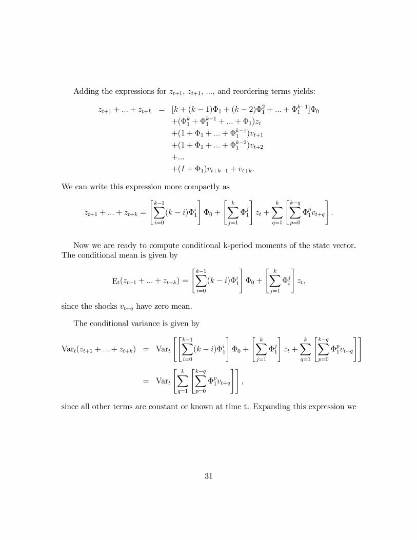
Adding the expressions for zt+1, zt+1, ..., and reordering terms yields:

zt+1 + ...+ zt+k = [k + (k − 1)Φ1 + (k − 2)Φ21 + ...+ Φk−11 ]Φ0

+(Φk1 + Φk−1

1 + ...+ Φ1)zt

+(1 + Φ1 + ... + Φk−11 )vt+1

+(1 + Φ1 + ... + Φk−21 )vt+2

+...

+(I + Φ1)vt+k−1 + vt+k.

We can write this expression more compactly as

zt+1 + ...+ zt+k =

"k−1Xi=0

(k − i)Φi1

#Φ0 +

"kX

j=1

Φj1

#zt +

kXq=1

"k−qXp=0

Φp1vt+q

#.

Now we are ready to compute conditional k-period moments of the state vector.The conditional mean is given by

Et(zt+1 + ... + zt+k) =

"k−1Xi=0

(k − i)Φi1

#Φ0 +

"kX

j=1

Φji

#zt,

since the shocks vt+q have zero mean.

The conditional variance is given by

Vart(zt+1 + ...+ zt+k) = Vart

""k−1Xi=0

(k − i)Φi1

#Φ0 +

"kX

j=1

Φj1

#zt +

kXq=1

"k−qXp=0

Φp1vt+q

##

= Vart

"kX

q=1

"k−qXp=0

Φp1vt+q

##,

since all other terms are constant or known at time t. Expanding this expression we

31

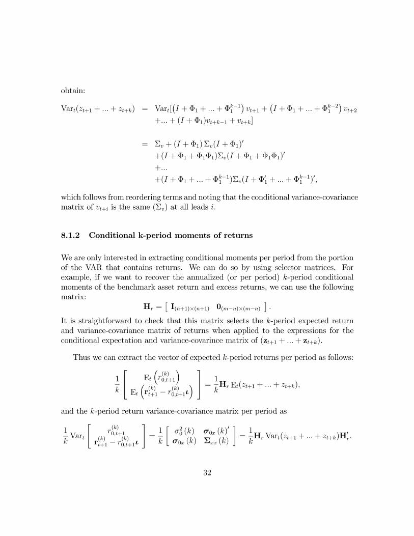
obtain:

Vart(zt+1 + ...+ zt+k) = Vart[¡I + Φ1 + ...+ Φk−1

1

¢vt+1 +

¡I + Φ1 + ... + Φk−2

1

¢vt+2

+... + (I + Φ1)vt+k−1 + vt+k]

= Σv + (I + Φ1)Σv(I + Φ1)0

+(I + Φ1 + Φ1Φ1)Σv(I + Φ1 + Φ1Φ1)0

+...

+(I + Φ1 + ...+ Φk−11 )Σv(I + Φ01 + ...+ Φk−1

1 )0,

which follows from reordering terms and noting that the conditional variance-covariancematrix of vt+i is the same (Σv) at all leads i.

8.1.2 Conditional k-period moments of returns

We are only interested in extracting conditional moments per period from the portionof the VAR that contains returns. We can do so by using selector matrices. Forexample, if we want to recover the annualized (or per period) k -period conditionalmoments of the benchmark asset return and excess returns, we can use the followingmatrix:

Hr =£I(n+1)×(n+1) 0(m−n)×(m−n)

¤.

It is straightforward to check that this matrix selects the k -period expected returnand variance-covariance matrix of returns when applied to the expressions for theconditional expectation and variance-covarince matrix of (zt+1 + ...+ zt+k).

Thus we can extract the vector of expected k-period returns per period as follows:

1

k

⎡⎣ Et

³r(k)0,t+1

´Et³r(k)t+1 − r

(k)0,t+1ι

´ ⎤⎦ = 1

kHr Et(zt+1 + ...+ zt+k),

and the k-period return variance-covariance matrix per period as

1

kVart

"r(k)0,t+1

r(k)t+1 − r

(k)0,t+1ι

#=1

k

∙σ20 (k) σ0x (k)

0

σ0x (k) Σxx (k)

¸=1

kHr Vart(zt+1 + ... + zt+k)H

0r.

32

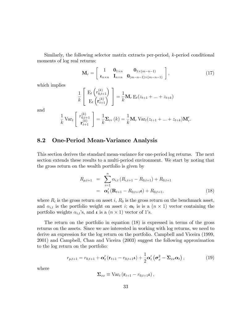
Similarly, the following selector matrix extracts per-period, k -period conditionalmoments of log real returns:

Mr =

∙1 01×n 01×(m−n−1)

ιn×n In×n 0(m−n−1)×(m−n−1)

¸, (17)

which implies

1

k

⎡⎣ Et ³r(k)0,t+1´Et³r(k)t+1

´ ⎤⎦ = 1

kMr Et(zt+1 + ... + zt+k)

and1

kVart

"r(k)0,t+1

r(k)t+1

#=1

kΣrr (k) =

1

kMr Vart(zt+1 + ... + zt+k)M

0r.

8.2 One-Period Mean-Variance Analysis

This section derives the standard mean-variance for one-period log returns. The nextsection extends these results to a multi-period environment. We start by noting thatthe gross return on the wealth portfolio is given by

Rp,t+1 =nXi=1

αi,t (Ri,t+1 −R0,t+1) +R0,t+1

= α0t (Rt+1 −R0,t+1ι) +R0,t+1, (18)

where Ri is the gross return on asset i, R0 is the gross return on the benchmark asset,and αi,t is the portfolio weight on asset i; αt is is a (n × 1) vector containing theportfolio weights αi,t’s, and ι is a (n× 1) vector of 1’s.The return on the portfolio in equation (18) is expressed in terms of the gross

returns on the assets. Since we are interested in working with log returns, we need toderive an expression for the log return on the portfolio. Campbell and Viceira (1999,2001) and Campbell, Chan and Viceira (2003) suggest the following approximationto the log return on the portfolio:

rp,t+1 = r0,t+1 +α0t (rt+1 − r0,t+1ι) +1

2α0t¡σ2x −Σxxαt

¢, (19)

whereΣxx ≡ Vart (rt+1 − r0,t+1ι) ,

33

andσ2x ≡ diag (Σxx) .

We now derive the one-period mean-variance frontier with and without a risklessasset, and the weights for the “tangency portfolio,” i.e. the portfolio containing onlyrisky assets that also belongs simultaneously to both the mean-variance frontier ofrisky assets, and the mean-variance frontier with a riskless asset.

8.2.1 One-PeriodMean-Variance Frontier with Log Returns and No Risk-less Asset

This section derives the mean-variance frontier when none of the assets available forinvestment is unconditionally riskless in real terms at a one-period horizon. Thishappens, for example, when there is significant short-term inflation risk, and the onlyshort-term assets available for investment are nominal money market instruments,such as nominal T-bills. In practice short-term inflation risk is small, and one canprobably ignore it. However, we still think it is worth analyzing the case with no one-period riskless asset, to gain intuition for the subsequent results for long horizons,where inflation risk is significant, and nominal bonds can be highly risky in real terms.

Problem We state the mean-variance portfolio optimization problem with log re-turns as follows:

minα

1

2Vart (rp,t+1) , (20)

subject to

Et (rp,t+1) +1

2Vart (rp,t+1) = µp,

where rp,t+1 is given in equation (19). That is, we want to find the vector of portfolioweights αt that minimizes the variance of the portfolio log return when the requiredexpected gross return on the portfolio is µp.

Equation (19) implies that the variance of the log portfolio return is given by

Vart (rp,t+1) = α0tΣxxαt + σ20 + 2α0tσ0x

34

and the log expected portfolio return is given by

Et (rp,t+1)+1

2Vart (rp,t+1) =

µEt r0,t+1 +

1

2σ20

¶+α0t

µEt (rt+1 − r0,t+1ι) +

1

2σ2x + σ0x

¶.

(21)

It is useful to note here that the VAR(1) model for returns given in equation (3)implies that

Et r0,t+1 = H00 (Φ0 +Φ1zt)

and

Et (rt+1 − r0,t+1ι) = Et (xt+1)

= Hx (Φ0 +Φ1zt) ,

where H00 is a (1×m) selection vector (1, 0, ..., 0) that selects the first element of the

matrix which it multiplies, and Hx is a (n×m) selection matrix that selects rows 2through n+ 1 of the matrix which it multiplies:

Hx =£0n×1 In×n 0(m−n−1)×(m−n−1)

¤,

where In×n is an identity matrix.

The Lagrangian for this problem is

L = 1

2Vart (rp,t+1) + λ

µµP −

µEt (rp,t+1) +

1

2Vart (rp,t+1)

¶¶,

where λ is the Lagrange multiplier on the expected portfolio return constraint. Notethat our definition of the portfolio return already imposes the constraint that portfolioweights must add up to one.

Mean-variance portfolio rule The solution to the mean-variance program (20)is

αt = λΣ−1xx

∙Et (rt+1 − r0,t+1ι) +

1

2σ2x + σ0x

¸−Σ−1xxσ0x. (22)

We can rewrite αt as a portfolio combining two distinct portfolios:

αt = λΣ−1xx

∙Et (rt+1 − r0,t+1ι) +

1

2σ2x

¸+ (1− λ)

¡−Σ−1xxσ0x¢ .35

The first portfolio is proportional to the expected gross excess return on all assets,weighted by the inverse of the variance-covariance matrix of excess returns. If assetreturns are independent of each other, so Σxx is a diagonal matrix containing thevariances of asset returns, this portfolio is simply the vector of Sharpe ratios for eachasset class–each one divided by its return standard deviation.

The second portfolio, with weightsΣ−1xxσ0x, is the portfolio of assets with minimumabsolute variance, or global minimum-variance portfolio. That is, this portfolio is thesolution to:

−Σ−1xxσ0x = minα

1

2Vart (rp,t+1) .

In the literature on dynamic optimal portfolio choice, the mean-variance portfoliois also known as the “myopic portfolio.” This name derives from the fact that it takesinto consideration only expected returns next period, ignoring other considerationsthat might affect the portfolio decisions of risk averse investors, such as the abilitythat certain asset classes might have to protect the spending needs of these investorsfrom a sudden deterioration in investment opportunities.

Equation for mean-variance frontier Equation (22) implies the following rela-tion between σ2p ≡ Vart(rp,t+1) and µp:

11

σ2p =1

A

¡eµ2p + 2Beµp +B2

¢+ σ20 − C, (23)

where eµp is the expected excess return on the portfolio over the benchmark asset,

eµp = µp −µEt r0,t+1 +

1

2σ20

¶,

and

A =

µEt (rt+1 − r0,t+1ι) +

1

2σ2x + σ0x

¶0Σ−1xx

µEt (rt+1 − r0,t+1ι) +

1

2σ2x + σ0x

¶,

B = σ00xΣ−1xx

µEt (rt+1 − r0,t+1ι) +

1

2σ2x + σ0x

¶,

C = σ00xΣ−1xxσ0x.

11To get this equation, note that at the optimum either λ = 0, or µP =¡Et (rp,t+1) +

12σ

2p

¢.

36

8.2.2 One-Period Mean-Variance Frontier with Log Returns and a Risk-less Asset

In this section we consider mean-variance analysis with log returns when investorshave an additional asset which is truly riskless in real terms over one period. Thisasset is an inflation-indexed T-Bill. We denote its return as rf . Thus the investorhas now n + 2 assets available for investment. This derivation is useful to computethe tangency portfolio.

Problem

minα

1

2Vart (rp,t+1 − rf) (24)

subject to Et (rp,t+1 − rf) +1

2Vart (rp,t+1 − rf ) = µp − rf ,

whererp,t+1 − rf = ω0t (rt+1 − rfι) +

1

2ω0t¡σ2r −Σrrωt

¢,

ωt is a (n+ 1)× 1 vector of portfolio weights,

Σrr ≡ Vart (rt+1 − rfι) ,

andσ2r ≡ diag (Σrr) .

The variance of the log excess portfolio return is given by

Vart (rp,t+1 − rf) = ω0tΣrrωt (25)

and the log excess expected portfolio return is given by:

Et (rp,t+1 − rf) +1

2Vart (rp,t+1 − rf) = ω0t

µEt (rt+1 − rfι) +

1

2σ2r

¶. (26)

Note that:Et (rt+1 − rfι) =Mr (Φ0 +Φ1zt)− rfι,

whereMr is the (n+ 1×m) selection matrix defined in (17).

37

The Lagrangian for this problem is

L = 1

2Vart (rp,t+1 − rf ) + λf

µµP − rf −

µEt (rp,t+1 − rf) +

1

2Vart (rp,t+1 − rf)

¶¶,

where λ is the Lagrange multiplier on the expected portfolio return constraint.

Mean-variance portfolio rule The solution to the mean-variance program (24)is

ωt = λfΣ−1rr

∙Et (rt+1 − rfι) +

1

2σ2x

¸. (27)

Equation for mean-variance frontier Equation (27) implies the following rela-tion between σ2p ≡ (Vart rp,t+1 − rf) and µp:

σ2p =1

Aeµ2p, (28)

where eµp is the expected excess return on the portfolio over the benchmark asset,

eµp = µp − rf

and

A =

µEt (rt+1 − rfι) +

1

2σ2r

¶0Σ−1xx

µEt (rt+1 − rfι) +

1

2σ2r

¶.

Equation (28) implies that, in a standard deviation-expected return space, the frontieris a line that intersects the expected return axis at rf , and it has a slope equal to√A. We show below that this slope is the Sharpe ratio of the tangency portfolio.

Tangency portfolio We can now derive the weights for the tangency portfolio be-tween frontiers (23) and (28). This is a portfolio whose weights ωT,t satisfy ω0T,tι = 1.That is, it is a portfolio with no loading on the risk-free asset.

We can easily solve for the weights of this portfolio by finding the Lagrange mul-tiplier λf for which ωt in (27) satisfies the constraint ω0T,tι = 1:

1 = ω0T,tι =λf

∙Et (rt+1 − rfι) +

1

2σ2r

¸0 ¡Σ−1rr

¢0ι,

38

which implies

λf =1£

Et (rt+1 − rfι) +12σ2r¤0Σ−1rr ι

.

Therefore,

ωT,t =1£

Et (rt+1 − rfι) +12σ2r¤0(Σ−1rr )

0 ιΣ−1rr

∙Et (rt+1 − rfι) +

1

2σ2r

¸. (29)

It is straightforward to show that the Sharpe ratio of the tangency portfolio equals√A, i.e., that the Sharpe ratio is the slope of the mean-standard deviation frontier

with a riskless asset. To see this, substitute (29) into equations (25) and (26) to com-pute expressions for the variance and expected excess return on the tangency portfolio,and compute the ratio of the expected excess return to the standard deviation.

8.3 Long-Horizon Mean-Variance Analysis

In this section we extend to a multiperiod horizon the results of Section 3 for mean-variance efficient allocations and frontiers. We assume that the investor has an in-vestment horizon of k periods, and that she chooses portfolio weights only every kperiods, i.e., at t, t+ k, t + 2k, .... We denote these weights as αt (k). The investorchooses those weights that minimize the variance per period of the log portfolio returnsubject to a required expected return per period on the portfolio.

To solve this problem we need to compute the log k-period portfolio return r(k)p,t+k.One possibility is to use, for similarity with the approximation for the log 1-periodportfolio return given in (19), the following expression:

r(k)p,t+k = r

(k)0,t+k +α0t (k)

³r(k)t+k − r

(k)0,t+kι

´+1

2α0t (k)

¡σ2x (k)−Σxx (k)αt (k)

¢, (30)

where ι is a (n× 1) vector of 1’s,

Σxx (k) ≡ Vart³r(k)t+k − r

(k)0,t+kι

´,

σ2x (k) ≡ diag (Σxx (k)) .

39

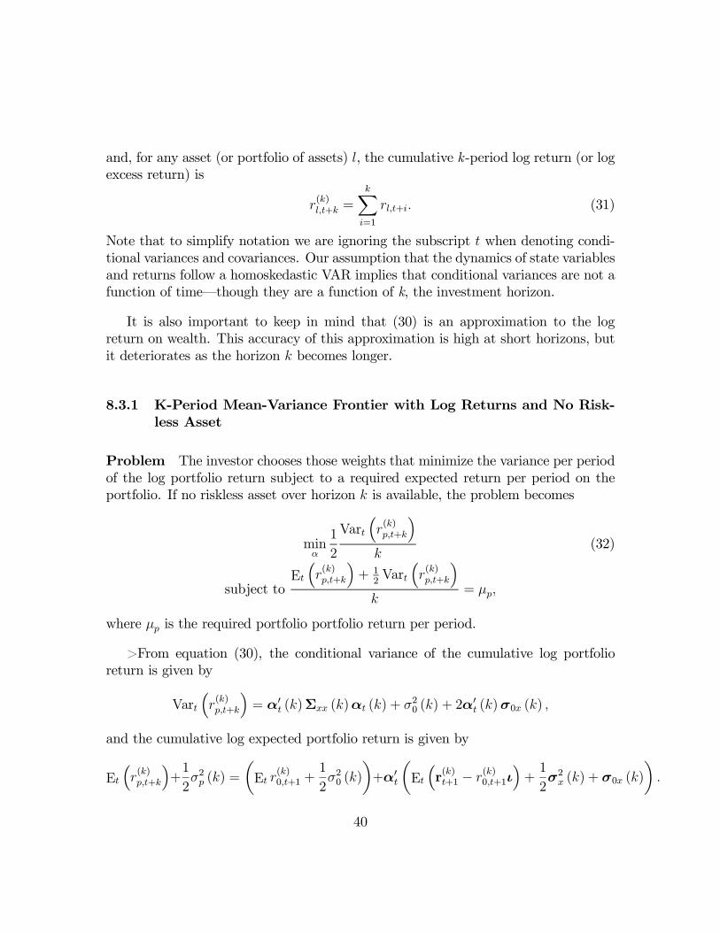
and, for any asset (or portfolio of assets) l, the cumulative k-period log return (or logexcess return) is

r(k)l,t+k =

kXi=1

rl,t+i. (31)

Note that to simplify notation we are ignoring the subscript t when denoting condi-tional variances and covariances. Our assumption that the dynamics of state variablesand returns follow a homoskedastic VAR implies that conditional variances are not afunction of time–though they are a function of k, the investment horizon.

It is also important to keep in mind that (30) is an approximation to the logreturn on wealth. This accuracy of this approximation is high at short horizons, butit deteriorates as the horizon k becomes longer.

8.3.1 K-Period Mean-Variance Frontier with Log Returns and No Risk-less Asset

Problem The investor chooses those weights that minimize the variance per periodof the log portfolio return subject to a required expected return per period on theportfolio. If no riskless asset over horizon k is available, the problem becomes

minα

1

2

Vart

³r(k)p,t+k

´k

(32)

subject toEt³r(k)p,t+k

´+ 1

2Vart

³r(k)p,t+k

´k

= µp,

where µp is the required portfolio portfolio return per period.

>From equation (30), the conditional variance of the cumulative log portfolioreturn is given by

Vart³r(k)p,t+k

´= α0t (k)Σxx (k)αt (k) + σ20 (k) + 2α

0t (k)σ0x (k) ,

and the cumulative log expected portfolio return is given by

Et

³r(k)p,t+k

´+1

2σ2p (k) =

µEt r

(k)0,t+1 +

1

2σ20 (k)

¶+α0t

µEt

³r(k)t+1 − r

(k)0,t+1ι

´+1

2σ2x (k) + σ0x (k)

¶.

40

Note that we already have expressions for the moments in the RHS of these equationsbased on our VAR specification.

The Lagrangian for this problem is

L = 1

2

Vart

³r(k)p,t+k

´k

+ λ

⎛⎝µP −Et

³r(k)p,t+k

´+ 1

2Vart

³r(k)p,t+k

´k

⎞⎠ ,

where λ is the Lagrange multiplier on the expected portfolio return constraint. Notethat we have already imposed the constraint that portfolio weights must add up toone in the way we define the log return on the portfolio.

Myopic portfolio rule The solution to the mean-variance program (20) is

αt (k) = λΣ−1xx (k)∙Et³r(k)t+1 − r

(k)0,t+1ι

´+1

2σ2x (k) + σ0x (k)

¸−Σ−1xx (k)σ0x (k) . (33)

Again, it is useful to note that we can write (33) as

αt (k) = λΣ−1xx (k)∙Et³r(k)t+1 − r

(k)0,t+1ι

´+1

2σ2x (k)

¸+ (1− λ)

¡−Σ−1xx (k)σ0x (k)¢ ,where Σ−1xx (k)σ0x (k) is the k-horizon global minimum-variance portfolio:

−Σ−1xx (k)σ0x (k) = minα

1

2Vart

¡rkp,t+k

¢.

Thus αt (k) is a linear combination of two portfolios, one of which is the globalminimum-variance portfolio.

Equation for k-period mean-variance frontier Equation (22) implies the fol-

lowing relation between σ2p (k) /k ≡ Vart³r(k)p,t+k

´/k and µp:

σ2p (k)

k=

1

A (k)

¡eµ2p + 2B (k) eµp +B2 (k)

¢+ σ20 (k)− C (k) , (34)

41

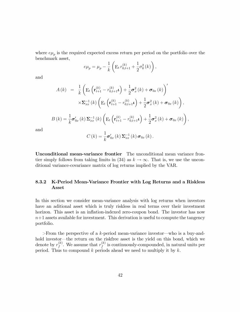
where eµp is the required expected excess return per period on the portfolio over thebenchmark asset,

eµp = µp −1

k

µEt r

(k)0,t+1 +

1

2σ20 (k)

¶,

and

A (k) =1

k

µEt

³r(k)t+1 − r

(k)0,t+1ι

´+1

2σ2x (k) + σ0x (k)

¶0×Σ−1xx (k)

µEt³r(k)t+1 − r

(k)0,t+1ι

´+1

2σ2x (k) + σ0x (k)

¶,

B (k) =1

kσ00x (k)Σ

−1xx (k)

µEt³r(k)t+1 − r

(k)0,t+1ι

´+1

2σ2x (k) + σ0x (k)

¶,

andC (k) =

1

kσ00x (k)Σ

−1xx (k)σ0x (k) .

Unconditional mean-variance frontier The unconditional mean variance fron-tier simply follows from taking limits in (34) as k →∞. That is, we use the uncon-ditional variance-covariance matrix of log returns implied by the VAR.

8.3.2 K-Period Mean-Variance Frontier with Log Returns and a RisklessAsset

In this section we consider mean-variance analysis with log returns when investorshave an aditional asset which is truly riskless in real terms over their investmenthorizon. This asset is an inflation-indexed zero-coupon bond. The investor has nown+1 assets available for investment. This derivation is useful to compute the tangencyportfolio.

>From the perspective of a k-period mean-variance investor–who is a buy-and-hold investor–the return on the riskfree asset is the yield on this bond, which wedenote by r(k)f . We assume that r

(k)f is continuously-compounded, in natural units per

period. Thus to compound k periods ahead we need to multiply it by k.

42

Problem

minα

1

2

Vart

³r(k)p,t+k − kr

(k)f

´k

(35)

subject toEt

³r(k)p,t+k − r

(k)f k

´+ 1

2Vart

³r(k)p,t+k − kr

(k)f

´k

= µp − r(k)f ,

where we assume that r(k)f is given in units per period, and r(k)l,t+k is defined in (31).

To solve this problem we need to compute the log k-period portfolio return r(k)p,t+k.We adopt the same convention as in the previous section, and use the k-period aheadconditional covariances for the Jensen’s inequality correction in the approximation tothe log excess return on wealth k periods ahead:

r(k)p,t+k − kr

(k)f = ω0t (k)

³r(k)t+k − kr

(k)f ι´+1

2ω0t (k)

¡σ2r (k)−Σrr (k)ωt (k)

¢, (36)

whereΣrr (k) ≡ Vart

³r(k)t+k − r

(k)f kι

´,

σ2r (k) ≡ diag (Σrr (k)) .

Using equation (36), the conditional variance of the cumulative log portfolio returnis given by

Vart³r(k)p,t+k − kr

(k)f

´= ω0t (k)Σrr (k)ωt (k) , (37)

and the cumulative log expected excess portfolio return is given by:

Et

³r(k)p,t+k − r

(k)f k

´+1

2Vart

³r(k)p,t+k − kr

(k)f

´= ω0t

µEt

³r(k)t+1 − r

(k)f kι

´+1

2σ2r (k)

¶.

(38)Note that we already have expressions for the moments in the RHS of these equationsbased on our VAR specification.

The Lagrangian for this problem is

L = 1

2

Vart

³r(k)p,t+k − kr

(k)f

´k

+λf

µµP − r

(k)f −

1

k

µEt³r(k)p,t+k − r

(k)f k

´+1

2Vart

³r(k)p,t+k − kr

(k)f

´¶¶,

where λf is the Lagrange multiplier on the expected portfolio return constraint. Notethat we have already imposed the constraint that portfolio weights must add up toone in the way we define the log return on the portfolio.

43

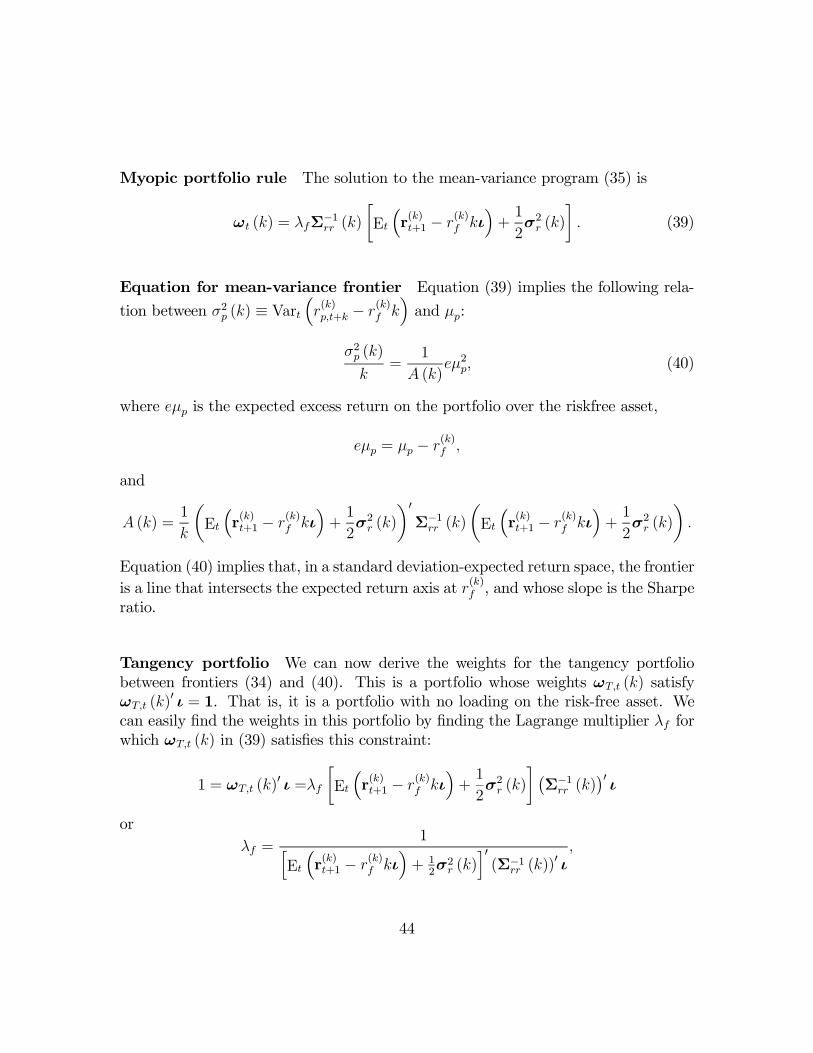
Myopic portfolio rule The solution to the mean-variance program (35) is

ωt (k) = λfΣ−1rr (k)

∙Et³r(k)t+1 − r

(k)f kι

´+1

2σ2r (k)

¸. (39)

Equation for mean-variance frontier Equation (39) implies the following rela-

tion between σ2p (k) ≡ Vart³r(k)p,t+k − r

(k)f k

´and µp:

σ2p (k)

k=

1

A (k)eµ2p, (40)

where eµp is the expected excess return on the portfolio over the riskfree asset,

eµp = µp − r(k)f ,

and

A (k) =1

k

µEt

³r(k)t+1 − r

(k)f kι

´+1

2σ2r (k)

¶0Σ−1rr (k)

µEt

³r(k)t+1 − r

(k)f kι

´+1

2σ2r (k)

¶.

Equation (40) implies that, in a standard deviation-expected return space, the frontieris a line that intersects the expected return axis at r(k)f , and whose slope is the Sharperatio.

Tangency portfolio We can now derive the weights for the tangency portfoliobetween frontiers (34) and (40). This is a portfolio whose weights ωT,t (k) satisfyωT,t (k)

0 ι = 1. That is, it is a portfolio with no loading on the risk-free asset. Wecan easily find the weights in this portfolio by finding the Lagrange multiplier λf forwhich ωT,t (k) in (39) satisfies this constraint:

1 = ωT,t (k)0 ι =λf

∙Et

³r(k)t+1 − r

(k)f kι

´+1

2σ2r (k)

¸ ¡Σ−1rr (k)

¢0ι

orλf =

1hEt

³r(k)t+1 − r

(k)f kι

´+ 1

2σ2r (k)

i0(Σ−1rr (k))

0 ι,

44

so that

ωT,t (k) =1h

Et³r(k)t+1 − r

(k)f kι

´+ 1

2σ2r (k)

i0(Σ−1rr (k))

0 ιΣ−1rr (k)

∙Et³r(k)t+1 − r

(k)f kι

´+1

2σ2r (k)

¸.

(41)

Once again, it is straightforward to show that the Sharpe ratio of the tangencyportfolio equals

pA (k), i.e., that the Sharpe ratio is the slope of the mean-standard

deviation frontier with a riskless asset. To see this, substitute (41) into equations(37) and (38) to compute expressions for the variance and expected excess return onthe tangency portfolio, and compute the ratio of the expected excess return to thestandard deviation.

45

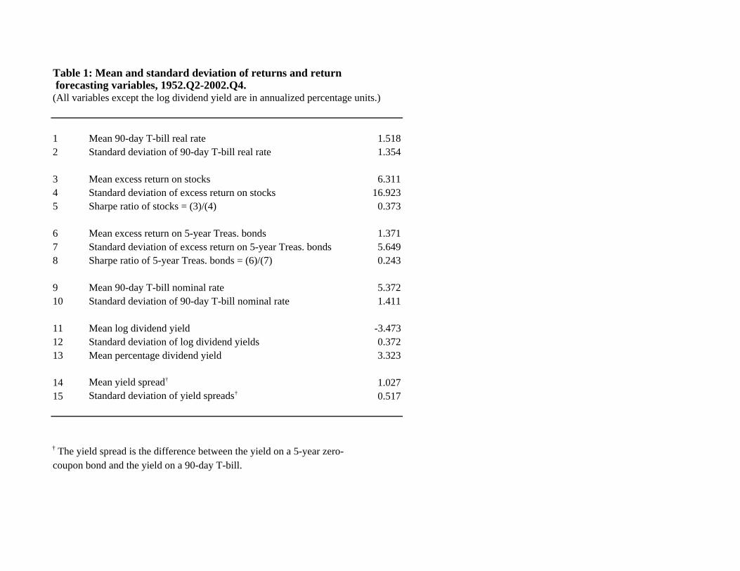
Table 1: Mean and standard deviation of returns and return forecasting variables, 1952.Q2-2002.Q4.(All variables except the log dividend yield are in annualized percentage units.)

1 Mean 90-day T-bill real rate 1.5182 Standard deviation of 90-day T-bill real rate 1.354

3 Mean excess return on stocks 6.3114 Standard deviation of excess return on stocks 16.9235 Sharpe ratio of stocks = (3)/(4) 0.373

6 Mean excess return on 5-year Treas. bonds 1.3717 Standard deviation of excess return on 5-year Treas. bonds 5.6498 Sharpe ratio of 5-year Treas. bonds = (6)/(7) 0.243

9 Mean 90-day T-bill nominal rate 5.37210 Standard deviation of 90-day T-bill nominal rate 1.411

11 Mean log dividend yield -3.47312 Standard deviation of log dividend yields 0.37213 Mean percentage dividend yield 3.323

14 Mean yield spread† 1.02715 Standard deviation of yield spreads† 0.517

† The yield spread is the difference between the yield on a 5-year zero-coupon bond and the yield on a 90-day T-bill.

Table 2: VAR estimation results, 1952.Q2-2002.Q4.

A. Slopes (t-statistics in parenthesis)R-squared

(1) (2) (3) (4) (5) (6)(1) log real T-bill rate 0.4029 0.0009 0.0002 0.2597 -0.0013 0.3999 0.299

(5.732) (0.167) (0.008) (3.493) (-1.211) (2.254)(2) log stock excess returns 1.0536 0.0268 0.3796 -2.1044 0.0549 -0.1348 0.095

(0.977) (0.380) (1.583) (-2.431) (3.021) (-0.056)(3) log bond excess returns -0.1088 -0.0568 -0.0686 0.3706 -0.0039 3.1252 0.097

(-0.374) (-2.672) (-0.583) (0.944) (-0.769) (3.169)(4) log nominal yield on T-bills -0.0023 0.0050 0.0027 0.9539 0.0003 0.0961 0.872

(-0.074) (2.315) (0.217) (22.262) (0.772) (1.084)(5) log dividend yield -1.2428 -0.0157 -0.3753 1.3617 0.9613 -0.3787 0.951

(-1.129) (-0.217) (-1.489) (1.518) (52.792) (-0.154)(6) log yield spread 0.0041 -0.0015 0.0029 0.0217 -0.0001 0.7596 0.561

(0.174) (-0.869) (0.378) (0.848) (-0.352) (13.160)

B. Quarterly percent standard deviations of residuals (diagonal) and cross-correlations of residuals (off-diagonal)

(1) (2) (3) (4) (5) (6)(1) log real T-bill rate 0.567 0.221 0.357 -0.349 -0.223 0.143(2) log stock excess returns 0.221 8.064 0.119 -0.101 -0.983 0.015(3) log bond excess returns 0.357 0.119 2.689 -0.755 -0.141 0.147(4) log nominal yield on T-bills -0.349 -0.101 -0.755 0.252 0.132 -0.754(5) log dividend yield -0.223 -0.983 -0.141 0.132 8.175 -0.042(6) log yield spread 0.143 0.015 0.147 -0.754 -0.042 0.172

Coefficients on lagged variables

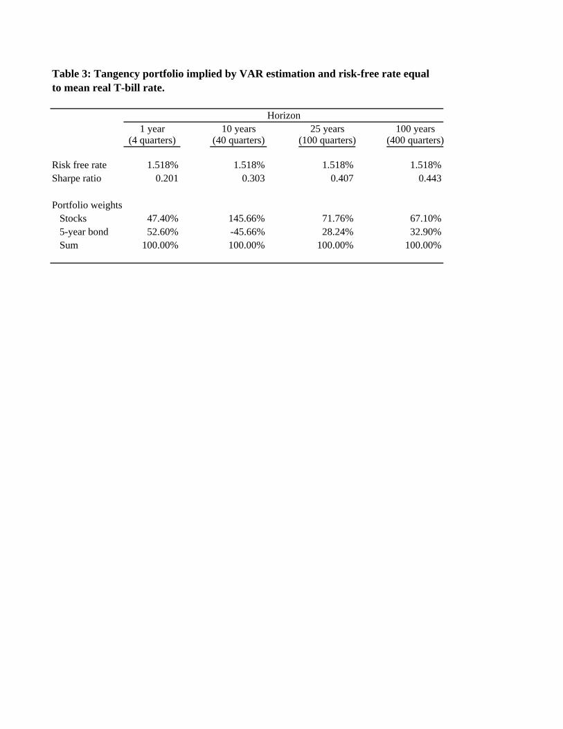
Table 3: Tangency portfolio implied by VAR estimation and risk-free rate equal to mean real T-bill rate.

1 year 10 years 25 years 100 years(4 quarters) (40 quarters) (100 quarters) (400 quarters)

Risk free rate 1.518% 1.518% 1.518% 1.518%Sharpe ratio 0.201 0.303 0.407 0.443

Portfolio weights Stocks 47.40% 145.66% 71.76% 67.10% 5-year bond 52.60% -45.66% 28.24% 32.90% Sum 100.00% 100.00% 100.00% 100.00%

Horizon

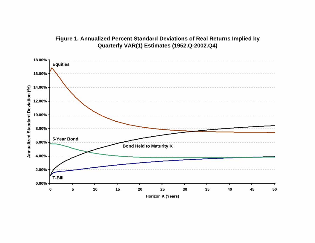
Figure 1. Annualized Percent Standard Deviations of Real Returns Implied by Quarterly VAR(1) Estimates (1952.Q-2002.Q4)

0.00%

2.00%

4.00%

6.00%

8.00%

10.00%

12.00%

14.00%

16.00%

18.00%

0 5 10 15 20 25 30 35 40 45 50

Horizon K (Years)

Ann

ualiz

ed S

tand

ard

Dev

iatio

n (%

)

Equities

5-Year Bond

T-Bill

Bond Held to Maturity K

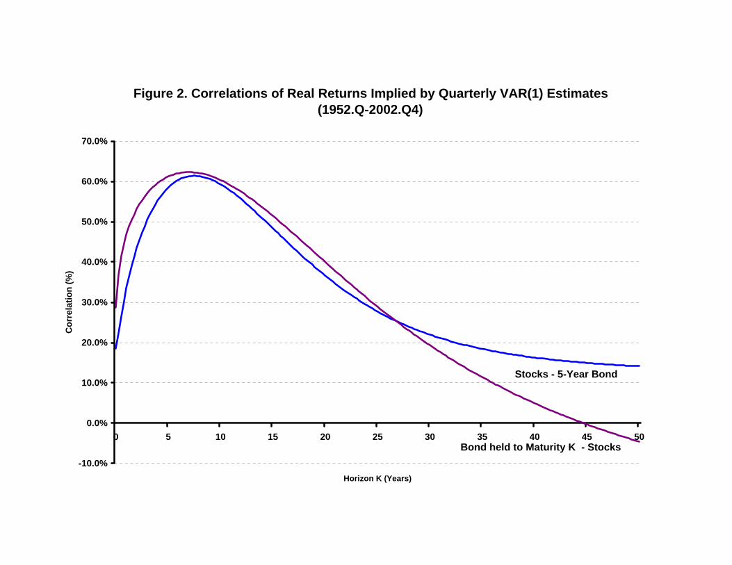
Figure 2. Correlations of Real Returns Implied by Quarterly VAR(1) Estimates (1952.Q-2002.Q4)

-10.0%

0.0%

10.0%

20.0%

30.0%

40.0%

50.0%

60.0%

70.0%

0 5 10 15 20 25 30 35 40 45 50

Horizon K (Years)

Cor

rela

tion

(%)

Stocks - 5-Year Bond

Bond held to Maturity K - Stocks

Figure 3. Risk of T-bills and Risk of the Global Minimum Variance Portfolio (GMV).

0.0%

0.5%

1.0%

1.5%

2.0%

2.5%

3.0%

3.5%

4.0%

4.5%

0 5 10 15 20 25 30 35 40 45 50

Horizon (Years)

Ann

ualiz

ed S

tand

ard

Dev

iatio

n (%

)

GMV

T-Bills

Figure 4. Composition of Global Minimum Variance Portfolio

-20.0%

0.0%

20.0%

40.0%

60.0%

80.0%

100.0%

120.0%

1 Quarter 5 Years 10 Years 25 Years 50 Years 100 YearsHorizon

Port

folio

Wei

ght (

%)

T-billsStocks5-year Bond