nc verification of up to 5 axis machining processes …
TRANSCRIPT
1
NC VERIFICATION OF UP TO 5 AXIS MACHINING PROCESSES USINGMANIFOLD STRATIFICATION
Karim Abdel-MalekDepartment of Mechanical Engineering and
Center for Computer Aided DesignThe University of Iowa
Iowa City, IA 52242Tel. (319) 335-5676 Fax. (319) 335-5669
Walter SeamanDepartment of Mathematics
The University of [email protected]
Harn-Jou YehMicrotek International
A numerically controlled machining verification method is developed based on a formulation fordelineating the volume generated by the motion of a cutting tool on the workpiece (stock).Varieties and subvarieties that are subsets of some Eucledian space defined by the zeros of afinite number of analytic functions are computed and are characterized as closed form equationsof surface patches of this volume. The motion of a cutter tool is modeled as a surfaceundergoing a sweep operation along another geometric entity. A topological space describingthe swept volume will be built as a stratified space with corners. Singularities of the variety areloci of points where the Jacobian of the manifold has lower rank than maximal. It is shown thatvarieties appearing inside the manifold representing the removed material are due to a lowerdegree strata of the Jacobian. Some of the varieties are complicated and will be shown to bereducible because of their parametrization and are addressed. Benefits of this method are evidentin its ability to depict the manifold and to compute a value for the volume.
1. INTRODUCTIONIn many applications such as solid modeling, collision detection, and manipulator workspaceanalyses, it is necessary to determine boundary surfaces to volumes swept by the motion of ageometric entity along another. Computer modeling and simulation used in the validation ofnumerically controlled (NC) machining programs before they are executed on a computer-controlled machine are known as NC verification.
While recent advances in this field have been made in terms of speed and accuracy, formulationsfor verifying more than 3 axes machining processes have been very limited. Early work on thissubject is due to Wang and Wang (1986). Works addressing the representation of the boundaryof the removed material have become of importance in recent years. For example, Boussac and
Abdel-Malek, K., Seaman, W., and Yeh, H.J., (2000), "NC Verification of up to 5 AxisMachining Processes Using Manifold Stratification" ASME Journal of Manufacturing Scienceand Engineering, Vol. 122, pp. 1-11.

2
Crosnier (1996) suggest a representation of swept volumes generated by the motion ofdeformable objects based on the topological properties of n-dimensional manifolds.
Methods of dual quadtree structures and boundary representation were applied to modeling theparts cut by a wire for Electric Discharge Machining (EDM) verification (Liu and Esterling1997). The Sweep envelope differential equation method is probably the most elegant methodto-date that has been shown to be suitable for NC verification (Blackmore, et al. 1997, and Leu,et al. 1997). Some of the works that have addressed NC verification but that have not used sweptvolume methods include Voelker and Hunt (1985), Menon and Voelcker (1992), Oliver andGoodman (1990), Narvekar, et al. (1992), Takata,et al. (1992), Jerard and Drysdale (1988 and1991), Koren and Lin (1995), Menon and Robinson (1993), Oliver and Goodman (1990) andOliver (1990), Narvekar, et al. (1992), Liang, et al. (1997), and Liu, et al. (1996).The work presented here is a culmination of many reports (Abdel-Malek and Yeh 1997a and1997b, Abdel-Malek, et al. 1997, and Abdel-Malek, et al. 1998) and presents them in anintegrated and generalized manner. The report by Abdel-Malek and Yeh (1997a) presented thefirst introduction of the Jacobian rank deficiency method. It was shown to treat consecutivesweep operations of up to four parameters. Further expanding this method, Abdel-Malek, et al.(1998) presented a complete rigorous mathematical formulation adapted from kinematics tostudy the acceleration function on singular surfaces. It was shown that definiteness properties ofa quadratic form can play an important role in identifying boundaries that admit no motion andhence are boundaries to the swept volume.
The expansion of this work into a broadly applicable formulation using methods fromdifferential geometry and differential topology are presented in this paper. This is the firstintroduction of the formulation for n-parameter sweeps where manifold stratification is essential.Furthermore, the adaptation of this work to numerically controlled verification has proven thatthe formulation is suitable for a variety of fields where sweeping is the underlying action.Manifold stratification and boundary identification are presented in detail.
There have been many works that have treated the topic of swept volumes and the reader isreferred to the references surveyed by Abdel-Malek and Yeh (1997a) and by Blackmore, et al.1997. More recent work that have demonstrated analytic methods for computing swept volumesare (Ahn, et al. 1997, Elber 1997, Ling and Chase 1996, Sourin and Pasko 1996).
Before proceeding with the analysis and to remain consistent with the terminology used indifferential geometry and differential topology (Spivak 1968, Guillemin and Pollack 1974, andLu, 1976), we define some terms that will be used throughout this work.Swept volume: The totality of points touched by a geometric entity while in motion.Variety: Subset of a Euclidean space defined by zeros of a finite number of differentiablefunctions.Manifold with singularities: A manifold with singular or boundary parts of lower dimensions:3, 2, and 1.Stratified space: A toplogical space which is built up from lower dimensional pieces that are
boundaryless manifolds.Strata: Plural of the Latin word stratum (layer or level).

3
Subvariety: Variety that is part of a “reducible” variety.
We shall first present a formulation for characterizing the topological space that is produced as aresult of the sweep of a geometric entity (representing the cutting tool) in space along its cuttingpath due to multiple axes motion. The goal is to identify the boundary to this “manifold withsingularities”. Identification of varieties associated with zeros of a finite set of analytic functionswill establish a stratified space. These zeros trace a locus of points where the sweep Jacobianhas lower rank than maximal and will be shown to comprise varieties. The stratification occursby studying the locus of points where the Jacobian has a fixed rank. The resulting boundary ofthe space that is nearly a manifold with singularities will be identified and its volume computed.It will be shown that this formulation allows for an exact computation of the volume, and hencethe accuracy of the verification process is very high.
2. FORMULATIONThe motion of a cutting tool in an NC milling or EDM process can be characterized as the sweepof a surface (enveloping the tool) along some path. Consider a geometric entity that envelops thecutting tool and is parametrized in terms of one or more variables as a ( )3 1× vector given by
G( )u , where u = [ ... ]u unT
1 , and where the tool can be represented as a curve, a surface, oran entity in n-dimensional space. In order to generalize the formulation, we shall also considerboundaries imposed on G( )u in the form of constraints on the parameters ui characterized by
inequality constraints in the form of u u uiL
i iU≤ ≤ . Because of the multi-axis operation of NC
machines, the tool surface will be swept several times, each along or about an axis. This pathwill be considered as a second geometric entity parametrized in terms of one or more variables asa ( )3 1× vector Y1 1( )v . This entity also has a boundary defined by v v vL U
1 1 1≤ ≤ . The manifoldgenerated by the sweep of G( ,..., )u un1 on Y1 1( )v is defined by the vector
N q q q q R u1 1 1 1 1( ) ( ) ( ) ( ) ( ) ( ) ( )= = +x y z v vT
G Y (1)
where N q1( ) = x y zT
and q is the vector of generalized coordinates defined by
q = =[ ... ] ...q q u u vnT
n
T
1 1 1 and R1 1( )v is the ( )3 3× rotation matrix defining the
orientation of the cutting tool. In fact, )(1 qN characterizes the set of all points that belong to themanifold. Another axis motion yields an expanded swept volume in the form of
N q R N q R R R2 2 2 1 2 2 2 1 2 1 2( ) ( ) ( ) ( )= + = + +v vY G Y Y (2)
where now q = [ ... ]u u v vnT
1 1 2 . Another axis motion yields a modified set defined byN R R R R R R3 3 2 1 3 2 1 3 2 3= + + +G Y Y Y (3)
The generalized case yields a space characterized by the vector function
x = x x x( ) ( ) ( )x y z T
, such that
x G Y Y( )q R R= +���
��� +
=
+
= +
+ −
=
+
+∏ ∏∑ii
n m
ii j
n m
jj
n m
n m1 1
1
1
(4)
where q u v= T T T, u = [ ... ]u un
T1 , and v = [ ... ]v vm
T1 . The aim is to identify this
space, its boundary, and to compute its volume which is material the removed.

4
To impose inequality constraints, it was shown that a constraint of the form q q qi i imin max≤ ≤ can
be transformed into an equation by introducing a new set of generalized coordinates λ i such thatq a bi i i i= + sin λ i n m= +1, ..., (5)
where a q qi i i= +( )max min 2 and b q qi i i= −( )max min 2 are the mid-point and half-range,respectively (Abdel-Malek and Yeh 1997a). At any point in the manifold, a vector constraintequation Φ( )*q with the parametrized inequality constraints can be defined as
F( )
( )
( )
( )
sin
*q
q
q
q0=
−−−
− −
�
!
"
$
####=
x
x
x
l
( )
( )
( )
x
y
z
i i i i
x
y
z
q a b
i n m= +1,..., (6)
where q u v* = T T T Tl is the vector of all generalized coordinates and l = +[ ... ]λ1 ln m
T .
Note that although ( )n m+ new variables (li ’s) have been added, ( )n m+ equations have alsobeen added to the constraint vector function without affecting the dimensionality of the problem.In order to have a well-posed formulation; constraints that are used to model the geometry of thisproblem should be independent, except at certain critical surfaces in the manifold (ImplicitFunction Theorem) when the Jacobian becomes singular. It is important, therefore, that there notbe open sets in the space of the generalized parameters in which the constraints are redundant.Redundancy occurs when the Jacobian F F
qq*
*= ∂ ∂ , is rank-deficient which will subsequently
define varieties in the manifold.
Candidate varieties forming the boundary of the manifold are identified by computing values thatcreate a locus of points where the Jacobian has lower rank than maximal. The stratificationoccurs by investigating the locus of points where the Jacobian has a fixed rank.
∂ ⊂ ≤W Rank k for some with ( ) =*F F
qq q q 0* ( ) ,* *J L (7)
where k is at most ( )2 2 1n m+ − . This process becomes more pressing as the number of theparameters increases. A manifold with variety or with corners that is built up from lowerdimensional pieces is described as a "stratified" space.
Including parameter limits F l( ( ))q , the rows of F F llqq q q= ∂ ∂ ∂ ∂ are dependent and
there exists a set of constants no
T= g g g1 2 3 that satisfy
Flqq n 0
T
o = (8)
Indeed, no is a vector normal to a tangent plane at a point in the space at which a tangent planeexists and was shown to be normal to a variety (Abdel-Malek and Yeh 1997a). The Jacobian isexpanded as

5
Fx
l
q
q 0
I q*
( ) ( ) ( )
( ) ( ) ( )
( ) ( ) ( )
...
...
...
cos ...
cos ...
... ... ... ...
... cos
= −−
−
�
!
"
$
#########
=�!
+
+
+
+ +
x x x
x x x
x x x
l
l
l
qx
qx
qx
qy
qy
qy
qz
qz
qz
n m n m
n m
n m
n m
b
b
b
1 2
1 2
1 2
0 0 0 0
0 0 0 0
0 0 0 0
1 0 0 0 0 0
0 1 0 0 0 0
0 0 1 0
0 0 0 1 0 0
1 1
2 2
"$# (9)
where the notation x qx
1
( ) denotes the partial derivative of ξ ( )x with respect to q1 , x xq q= ∂ ∂ is
the upper left corner sub-matrix (only with respect to q ), q ql
l= ∂ ∂ is the diagonal lower rightcorner matrix and I is the identity matrix.
For an ( )n m+ -parameter verification, the Jacobian Fq
q* ( )* row-rank deficiency yields three
types of singular bahavior. Criterion (i) In order to make the matrix x q rank deficient of order (d), it is necessary to
determine all square sub-Jacobians which are analytic functions. Equating the determinantsto zero yields a number of analytic equations to be solved simultaneously. The zeros of theresulting equations are sets of constant generalized coordinates denoted by pi and arecharacterized by the following set
p 0i
i j k
i j k
i j k n m i j k=�
!
"
$###
= = + ≠ ≠
%&K
'K
()K
*K
det( )
:
det( )
, ,...,
h h h
h h h
1
1
η
for , , and i = 1 2, ,...,β (10)
where hi denotes a column of the matrix x q = [ ... ]h hk m , β is the number of singular
sets, and pi is a subset of q such that q p sTiT T= , i.e., s contains the remaining non-
constant generalized coordinates.Criterion (ii) If the matrix q
l is row-rank deficient (i.e., bi icosλ is zero for some
i n m= +1,...,( ) then qi has reached a limit and the corresponding ξq is studied for row-rank
deficiency. When certain parameters reach their limits, e.g., q q q q q qi j k i j k, , , ,= limit limit limit , the
corresponding diagonal elements in the matrix ql will be equal to zero. For example, if
q qi i= min (or qimax ), the diagonal element of qλ will be zero (i.e., bi icosl is zero for either
i n= 1 2,..., then qi has reached a limit). Therefore, the corresponding ∂
∂qq[ ( , )]x qi is subjected
to the rank-deficiency criterion such that the rank of Fq* will depend on the following matrix
x x x x xq q q q qi j k n m1
0 1 0 0 0
0 0 1 0 0
0 0 0 1 0
... ...
... ...
... ...
... ...
+�
!
"
$
####(11)

6
Solving the rank deficiency condition for Eq. 11 is equivalent to solving the rank deficiency for
x x x xq ⊄ [ , , ]q q qi j k, with q q q q q qi i j j k k= = =limit limit limit, , (12)
where the notation of ⊄ represents the exclusion of the right matrix from the left. Define a new
vector ∂qlimit limit limit limit= q q qi j k
T, , which is a sub-vector of q where 1 3≤ ≤ −dim ( )∂qlimit2 7 n .
Coordinates can be partitioned as q w q= ∂T T, limit , and φ∂ =∩ limitqw . Then, if [xw w q( , )]∂ limit
is row rank deficient, the sub-Jacobian x q is also rank deficient. Let the solution for this
condition be denoted by $p , which is a constant sub-vector of w, and w u p= T T T, $ . The type II
singularity set is defined asS n( ) [ $ ]: [ ( , )] , $ , ( ) ( )2 3 3≡ = ∪ < ∈ ≤ −p p q w q p w dim qq∂ ∂ ∂limit limit limit Rank for some x= B (13)
As for the case of dim ( )∂qlimit2 7 = −n 2 , i.e., only two generalized variables are allowed to vary
in their ranges, dim( )w = 2 , and the sub-matrix xw will be of dimension ( )3 2× , i.e., alreadyrow rank deficient. For this case, a type-III singularity is defined as
S q qn mi j
( ) ( ): [ , ,...]3 2≡ ∈ℜ ≡ =+ −p p q limit limit limit∂= B (14)
Substituting the set pi into the vector function x( )q yields a variety parametrized in terms of theremainder variables (characterized by s) as
x x( , ) ( )p s si = (15)subject to the constraints of the generalized coordinates s a bi i i i− − =sinλ 0 , where s is a subset
of q such that q p s= iT T T
. The vector function of Eq. (15) is a subvariety of the manifold
whose Jacobian is either full rank or rank deficient. Those that are already rank deficient areidentified as reducible varieties and can be further stratified. This process is explained below.
3. MANIFOLD STRATIFICATIONThe above formulation often yields some surfaces ∈R 3 with a parameterization of threevariables and are rank deficient. This indicates that the parameterization is not one-to-one andthat, as can be readily shown, the Jacobian of these entities is already rank deficient.
Since the rank-deficiency of this variety is of order one, it yields two constant generalizedcoordinates, i.e., one-parameter geometric entities. Curves instead of surfaces that identify theboundary are determined. For this case when x ei i i( ): ( )s s ∈ℜ → ℜ3 3 , where ε is the
corresponding vector of slack variables e = λ λ λk m
T
l, the Jacobian of the variety is
x xe e
= ss (16)
For a parameter at its limit ( )qilimit , the second block matrix of Eq. (16) is rank deficient. An
elementary matrix of row operations Ei applied to se
yields a row echelon form such that
E s Ei REe= (17)

7
where E1
0 1 0
0 0 1
0 0 0
=�
!
"
$###
, E2
1 0 0
0 0 1
0 0 0
=�
!
"
$###
, and E3
1 0 0
0 1 0
0 0 0
=�
!
"
$###; where the subscript denotes the
parameter number, and ERE is a row echelon form. This same matrix applied to ξ sT
yields
E0si
Tx
L=
�!
"$# (18)
where L L L L= 1 2 3 (19)
where dim( ) ( )L = ×2 3 and dim( ) ( )L j = ×2 1 for j = 1 2 3, , . The rank deficiency condition is
applied again to L . Solutions to the three equations are singular sets denoted by γ i such that
g g gi i i i
D
D
D
=�
!
"
$###
= ∈ ∩%&K'K
()K*K
1
2
3
0 s, , for = b φ (20)
where D1 1 2= L L , D2 2 3= L L , and D3 1 3= L L subject to the parameter constraints and
where γ i is a subset of s such that siT
iT
i= g β , where βi is the remaining variable such that
x g ki i i i i( , ) ( )β β= (21)where k i i( )b is a parametric space curve and dim( ( )) ( )k β = ×3 1 which represent boundary
curves to the variety ξ( )s . This submanifold is characterized by the varieties x( )s subject toκ( )β . Determination of the boundary to the manifold is addressed in the following section.
4. BOUNDARY VARIETIESIn order to distinguish regions of a variety that are part of boundary of the manifold, a second-order criterion is introduced. The Jacobian is not enough but it will be shown that a form of theHessian will identify such a boundary. Consider a point P on a smooth variety with a knownvector normal (note that this is only possible because of the capability of this formulation toobtain closed form equations of the varieties). This point may admit motion in either normaldirection to the variety. This motion depends on the difference between the component ofacceleration in the normal direction and the centripetal acceleration due to its tangential velocity.An indicator characterizes the difference (which is true for the general motion of a particle on acurve or surface (Abdel-Malek, et al. 1998)), such that
η ηρP P n
t
o
H av= = −( )
2
(22)
where vt is the tangential velocity, an is the component of acceleration in the normal directionto the variety, and 1 ρo is the normal curvature of the variety with respect to the tangentdirection of vt (ρ o is the radius of curvature). At a boundary, ηP will only indicate motiontowards the interior of the manifold. It will be shown that these boundaries do not admit motionregardless of the values of velocity or acceleration at the point of interest, but will only dependon the definiteness properties of a quadratic form.

8
In order to apply Eq. 22 to varieties x( )s , we define the Time-Modified First and SecondFundamental Forms (Farin 1993), denoted by ′I p and II′p , respectively,
′ ≡I s ss spT T
& &x x (23)
II s n sss
′ ≡pT T
& &x (24)
such that the normal curvature is still defined by Ko o p p= = ′ ′1 ρ II I (note that fundamental
forms are extensively used in differential geometry (Farin 1993)). In general, the tangentialvelocity in terms of x or F at any point on the surface is
v s qs qt = =x F& & (25)
where & &q q=ll . The squared norm of the velocity is v v v s ss st t
Tt
T T2 = = & &x x which is equal to the
Time-Modified First Fundamental Form ′I p . Therefore, ′I p can be written as ′ =I p tv2.
Substituting for 1 ρo and for ′I p into η yields
η = − ′ ′ = − ′a v an t p p n p
2II I II3 8 (26)
which indicates that time-modified second fundamental form is indeed the centripetalacceleration for a point on a variety. We will first evaluate an expression for II′p , followed by an
expression for an to obtain the indicator η .
4.1 Determining the Centripetal accelerationSince an is in terms of &q and to express II′p in terms of &q , the velocity vector (&s ) on a variety
is extracted from Eq. 25. Since x s is not square, a generalized inverse can be written such that
& &
&s B q B qq q= =F F ll
(27)
where B is the generalized inverse defined by B E Es= −x
1 and E =
�!
"$#
1 0 0
0 1 0 if the first and
second rows of x s are independent, E =�!
"$#
1 0 0
0 0 1 if the first and third rows are independent and
E =�
!
"
$#
0 1 0
0 0 1 if the second and third rows are independent. Substituting the expression for &s into
Eq. 24 yields
II s n sss
′ =pT T
& &x = & &l F x F ll l
T T Tq B n B qq ss q (28)
which is a general expression for II′p .
4.2 Determining the Component of Normal AccelerationDifferentiating Eq. 25 again with respect to time and using indicial form, the acceleration at anypoint is
&& & & &&xF
ll
F
ll
F
lli
i
j
j
kk
i
j
j
kk
i
j
j
kk
d
dt
d
dq
dq
d
d
dq
d
dt
dq
d
d
dq
dq
d=
�!
"$##
+�!
"$##
���
��� +
�!
"$##
(29)
Expanding the derivatives and collecting similar terms yields

9
&& & & &&x lF
l
F
l ll
F
lli n
j
n
i
m j
j
k
i
j
j
n kk
i
j
j
kk
dq
d
d
dq dq
dq
d
d
dq
d q
d d
d
dq
dq
d=
�!
"$##
+%&K'K
()K*K
+�!
"$##λ
2 2
(30)
In matrix form, Eq. 30 is written as
&& & & &&x l FF
l F ll l ll l
= + ⋅%&'
()* +=
+
∑q q qqq qT
ii
i
n m d
dqq
1
(31)
To obtain the normal acceleration, &&x is projected onto no . Recall that no is a vector normal to
the variety. Multiplying both sides of Eq. 31 by the vector noT eliminates the last term of the
right hand side (definition of the normal as the basis of the null space in Eq. 8).
The component of the normal acceleration is thenan o
T T= =n H&& & &
*x l l (32)
where H q q n qn
*( , )(
o oT
oT o
T
ii
i
n d
dqql F
F
l l ll= + ⋅
=∑ )
1
(33)
4.3 A Form of the Hessian MatrixTo compute a value for the indicator (η ), substitute for an (from Eq. 33) and for II′p (from Eq.
28) into Eq. 26, such thatη = − ′ =an
TII Qp& &
*l l (34)
where Q H q B n B qq ss q* = −∗
l lF x FT T T T (35)
where Q* is the quadratic matrix. Definiteness properties of the quadratic form of Eq. 35determines whether a variety admits motion in the direction of nT at a specified point (i.e.,
independent of the value of &λ ). This form will indicate if a region on a variety is a part of theboundary of the manifold, or is boundary to a void since no motion will be admitted in thedirection of the exterior of the manifold (including voids). If Q* is indefinite, the variety admitsmotion along either normal direction and is not a boundary.
For the case when q qi i= limit (at the boundary of a sweep or at the boundary of an entity), Eq. 35yields a semi-definite quadratic form. For this case, we propose the projection of a variationalmovement δ δF F= q ii
q due to δqi onto the normal direction n such that the normal component
is given bys = nT
q iiqF δ (36)
where δqi is a specified magnitude of ±1 as follows
δqq
qii
i
=+−
%&'1
1
if is at lower bound
if is at upper bound(37)
Positive values of s in Eq. 36 indicate that the variety can admit motion in the positivedirection of n. A boundary is established when an enclosure is identified as having admissibleoutput directions for all points on its boundary directed towards the interior of that enclosure asillustrated in Fig. 1. A void is identified as an enclosure that exhibits admissible directionstowards the exterior of the manifold. The algorithm is presented in Appendix A.

10
External boundary
voids
Admissibledirections
Manifold
Fig. 1 Identifying the boundary using admissible directions
5. AN INTRODUCTORY EXAMPLEConsider the NC verification of a process involving the motion of a cutting tool represented by acylindrical surface (two parameters) along a cutting path (a curve of one parameter) to generate amanifold in three parameters. The cylindrical surface is given by
G( ) cos sinu = − −10 20 102 1 2u u uT
(38)
with the following geometric constraints 0 201≤ ≤u and 0 22≤ ≤u π . The orientation of the
motion is defined by the matrix
−
−=
0cossin
100
0sincos
)(
11
11
1
vv
vv
vR subject to π π/ 4 5 41≤ ≤v and
Ψ( )vT
1 0 0 0= . The manifold is characterized by 3 parameters
x( )
cos cos sin sin
sin
cos cos cos sin
q =+ +
−− − +
�
!
"
$###
10 20
10
20 10
3 5 3 4 3
5
3 4 3 5 3
q q q q q
q
q q q q q
(39)
where q = q q qT
3 4 5 . Note that we have used the indices 3, 4, and 5 in order to simplify the
continuation of this example in the following section. The limits are parametrized asq3 33 4 2= +( ) ( ) sinπ π λ , q4 410 10= + sinλ , and q5 5= +π π λsin . The boundary to ξ( )q isto be determined. The Jacobian is computed as the matrix
Fq =
+ − −−
+ + − −−
−−
�
!
"
$
#######
20 10 10 0 0 0
0 0 10 0 0 0
10 20 10 0 0 0
1 0 0 2 0 0
0 1 0 0 10 0
0 0 1 0 0
3 4 3 5 3 3 3 5
5
3 5 3 4 3 3 3 5
3
4
5
cos cos cos sin sin cos sin
cos
cos cos sin sin cos sin sin
( / ) cos
cos
cos
q q q q q q q q
q
q q q q q q q q
π λλ
π λThe criteria are applied to the upper ( )3 3× corner matrix ξq which is square. Therefore, the
rank-deficiency criteria are applied by computing the zeros of the determinant of ξq as
x q = − + + =10 20 032
5 4 32
5 32
4 5 32( (cos ) cos (cos ) cos (sin ) cos (sin )q q q q q q q q q (40)
11
which can be simplified to x q = − + =10 20 04 5( ) cosq q . Solutions that satisfy x q = 0 are
cosq5 0= , (i.e., q5 3 2= π , q5 2= π ) and q4 20= − . Only p1 5 3 2= =q π; @ , and
p2 5 2= =q π; @ are considered since they satisfy the inequality constraints.
Rank deficiency conditions imposed on the matrix ql yield five other singularities as
p3 3 4= =q π; @ , p4 3 5 4= =q π; @ , p5 4 0= =q; @ , p6 4 20= =q; @ , and p7 5 0= =q; @ .
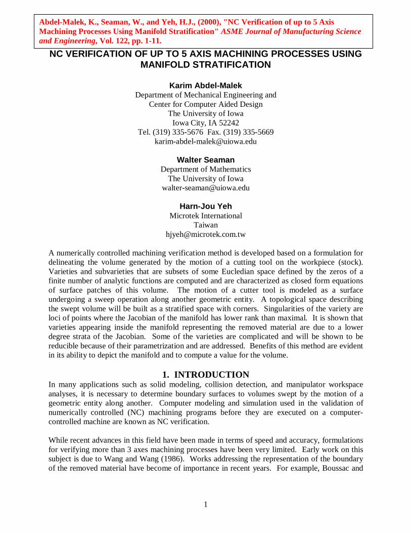
Substituting these singularities into Eq. (39) yields parametric equations of varieties. Forexample, substituting p2 5 2= =q π; @ into Eq. (39) yields the following variety
x( ) =s2 3 4 3 3 4 320 10 20sin sin cos cosq q q q q qT+ − − − (41)
where s2 3 4= q qT
. Similarly, for p1 3 5 4= =q π; @ , the equation is generated and varieties
for both p1 and p2 are shown in Fig. 2a. Varieties due to p3 and p4 are shown in Fig. 2b and
those due to p p6 and 7 are shown in Fig. 2c (Note that varieties are shown using Mathematica
using the parametric plot 3D capabilities).
Fig. 2 Varieties due to (a) p p p1, 2, 7 (b) p p3 , 4 and (c) p p5 , 6
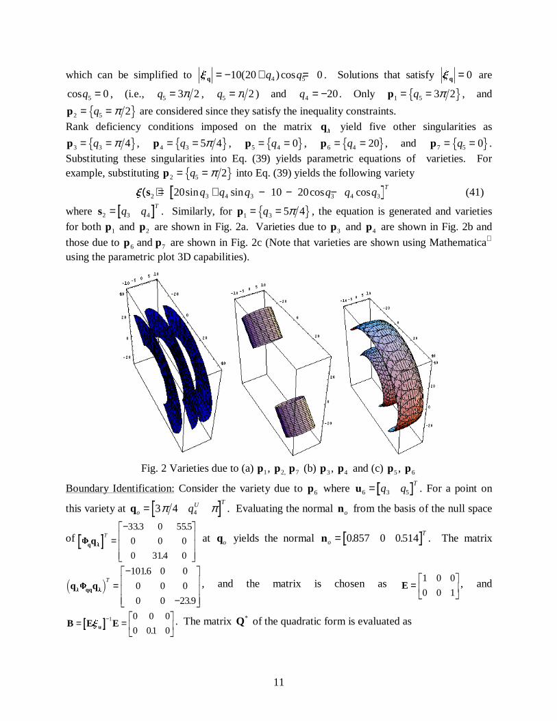
Boundary Identification: Consider the variety due to p6 where u6 3 5= q qT
. For a point on
this variety at qoU T
q= 3 4 4π π . Evaluating the normal no from the basis of the null space
of Flqq
T=
−�
!
"
$###
333 0 555
0 0 0
0 314 0
. .
.
at qo yields the normal no
T= 0857 0 0 514. . . The matrix
q qqql lF3 8T
=−
−
�
!
"
$###
1016 0 0
0 0 0
0 0 23 9
.
.
, and the matrix is chosen as E =�!
"$#
1 0 0
0 0 1, and
B E Eu= =�!
"$#
−x
1 0 0 0
0 01 0.. The matrix Q* of the quadratic form is evaluated as

12
Q* .= −�
!
"
$###
0 0 0
0 9 69 0
0 0 0
The eigenvalues of Q* are evaluated as −9 69 0. , , 0; @ , which indicates a negative semi-definite
quadratic form. Since q4 is at its upper bound ( qU4 ), the additional value of σ is evaluated with
δq4 1= − . The value for s = = −nTq qF
4 4 0 97δ . . Since the sign of s is the same as that of the
eigenvalues of Q* , it indicates that the surface x 6 at qo only admits motion in the opposite
direction of the normal no (towards the interior of the manifold).
Consider now the cylindrical surface at the start of the sweep operation with p3 3 4= =q π; @ at
qoLq q q= = =3 4 510, , π< A as shown in Fig. 3, the eigenvalues are − −1952. , , - 47.12 0.6; @ and
therefore, no motion towards the exterior occurs.
qoLq q q= = =3 4 510, , π< A qo
Lq q q= = =3 4 510 18, , . π< A
Fig. 3 The variety ξ3
However, on that same surface, at the opposite side at qoLq q q= = =3 4 510 18, , . π< A , the
eigenvalues are 37 9 0. , , 0.027 ; @ which is an indefinite form. The indicator s = −2418. is
different in sign from the nonzero eigenvalues, therefore admitting motion; i.e., this surface,although it does not admit motion along some regions, it does on another region interior to themanifold. The complete boundary to the manifold is identified and shown in Fig. 4.

13
Fig. 4 Volume removed6. FIVE-PARAMETER NC VERIFICATION
Consider the motion of the same cutting tool represented in the introductory example by acylindrical surface such that a 5-parameter verification will be developed. The machiningoperation will sweep the cylindrical surface first along the curve given above to yield theaccessible set now called G (Eq. 39) such that
G( , , )
cos cos sin sin
sin
cos cos cos sin
q q q
q q q q q
q
q q q q q3 4 5
3 5 3 4 3
5
3 4 3 5 3
10 20
10
20 10
=+ +
−− − +
�
!
"
$###
(42)
The first will be a rotational motion of Γ and the second will be a translation along an axis. Theresult is a sweep of Γ along a cylindrical surface defined by the rotation matrix
−=
100
0cossin
0sincos
)( 22
22
2 qq
qR and Y = 0 0 0T
(43)
followed by a translation with R I( )q1 = and Y( )q qT
1 10 0 30= + subject to the following
constraints 0 201≤ ≤q , π π/ 4 7 42≤ ≤q , π π/ 4 5 43≤ ≤q , 0 204≤ ≤q , and 0 25≤ ≤q π . Thetotality of points characterizing the manifold is given by the vector function
x( )
cos cos cos sin sin cos sin cos sin
sin cos cos cos sin sin sin sin sin
sin cos cos cos
q =+ + +− + +
− − + +
�
!
"
$###
10 10 20
10 10 20
10 20 30
2 3 5 2 5 2 3 4 2 3
2 3 5 2 5 2 3 4 2 3
3 5 3 4 3 1
q q q q q q q q q q
q q q q q q q q q q
q q q q q q
(44)
where q = q q q q qT
1 2 3 4 5 . The ( )3 5× upper sub-Jacobian of x q is computed as
xq =− + − −
+ + +�
!
0 10 10 20
0 10 10 20
1 0
2 3 5 2 5 2 3 4 2 3
2 3 5 2 5 2 3 4 2 3
sin cos cos cos sin sin sin sin sin
cos cos cos sin sin cos sin cos sin
q q q q q q q q q q
q q q q q q q q q q
14
− + + − +− + + − −
+ + − −
10 20 10 10
10 20 10 10
10 20 10
2 3 5 2 3 4 2 3 2 3 2 3 5 2 5
2 3 5 2 3 4 2 3 2 3 2 3 5 2 5
3 5 3 4 3 3 3 5
cos sin cos cos cos cos cos cos sin cos cos sin sin cos
sin sin cos sin cos sin cos sin sin sin cos sin cos cos
cos cos sin sin cos sin sin
q q q q q q q q q q q q q q q
q q q q q q q q q q q q q q q
q q q q q q q q
(45)
and the lower corner matrix is
qll( )
cos
cos
cos
cos
cos
=
−−
�
!
"
$
######
10 0 0 0 0
0 3 4 0 0 0
0 0 2 0 0
0 0 0 10 0
0 0 0 0
1
2
3
4
5
l
l
l
l
l
ππ
π
1 61 6 (46)
Criterion (i): Since (n m+ =) 5 and dim( )x q = ×3 5, there are ten ( )3 3× square sub-Jacobians
whose analytic determinants need to be determined. The resulting nonlinear equations are asfollows.j q q q q q q q q q q1 100 200 404
23 3 3 5
23 5 4 3 3= − + + −sin cos cos (cos ) sin cos sin cos
− − + − =400 400 10 20 032
5 3 3 4 5 4 32
5(cos ) cos sin cos cos (cos ) cosq q q q q q q q q
j q q q q q q2 10 20 20 03 3 5 32
4 32= − − + − =sin cos cos (cos ) (cos )
j q q q q q q q q q q q q q3 100 200 10 100 032
5 5 3 3 5 4 3 3 5 4 5 5= + + − =(cos ) cos sin sin cos sin sin cos sin cos sin
j4 0= and j q q q q q q q5 100 200 10 052
3 3 5 4 5 3= − − =(cos ) sin cos cos cos cos
j q q6 10 03 5= − =sin cos and j q q q q q q q q q q7 400 10 200 40 03 4 5 3 3 5 4 3 42
3= + + + + =sin cos cos cos cos sin sin
j8 0= and j q q q q q9 10 200 04 5 3 3 5= + =sin sin sin sin and j q q q10 200 10 05 4 5= − − =cos cos
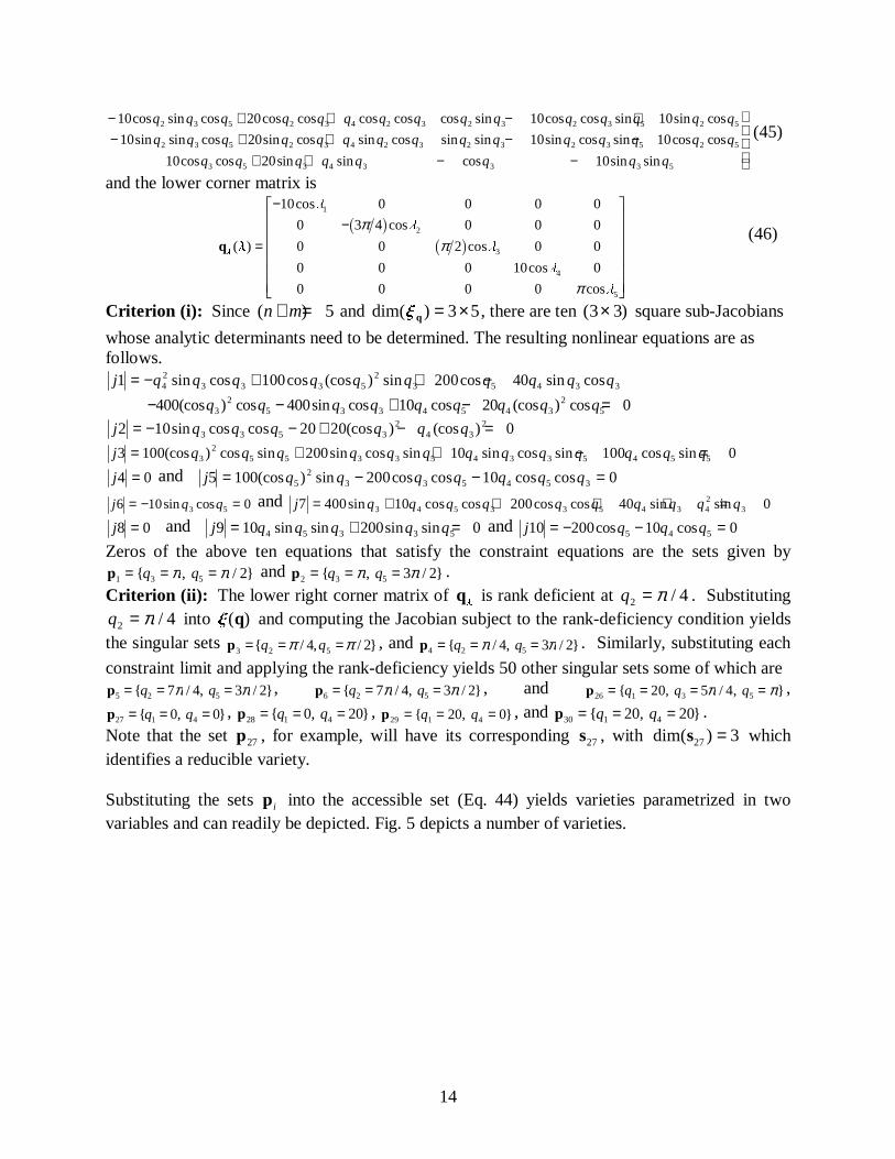
Zeros of the above ten equations that satisfy the constraint equations are the sets given byp1 3 5 2= = ={ , / }q qπ π and p2 3 5 3 2= = ={ , / }q qπ π .Criterion (ii): The lower right corner matrix of q
l is rank deficient at q2 4= π / . Substituting
q2 4= π / into x( )q and computing the Jacobian subject to the rank-deficiency condition yieldsthe singular sets }2/,4/{ 523 ππ === qqp , and p4 2 54 3 2= = ={ / , / }q qπ π . Similarly, substituting each
constraint limit and applying the rank-deficiency yields 50 other singular sets some of which arep5 2 57 4 3 2= = ={ / , / }q qπ π , p6 2 57 4 3 2= = ={ / , / }q qπ π , and p26 1 3 520 5 4= = = ={ , / , }q q q π π ,
p27 1 40 0= = ={ , }q q , p28 1 40 20= = ={ , }q q , p29 1 420 0= = ={ , }q q , and p30 1 420 20= = ={ , }q q .Note that the set p27 , for example, will have its corresponding s27 , with dim( )s27 3= whichidentifies a reducible variety.
Substituting the sets pi into the accessible set (Eq. 44) yields varieties parametrized in twovariables and can readily be depicted. Fig. 5 depicts a number of varieties.

15
Fig. 5. Varieties due to (a) p p63 65, (b) p p71 72,
Fig. 5. Varieties due to (c) p p79 86− and (d) p p31 38−
16
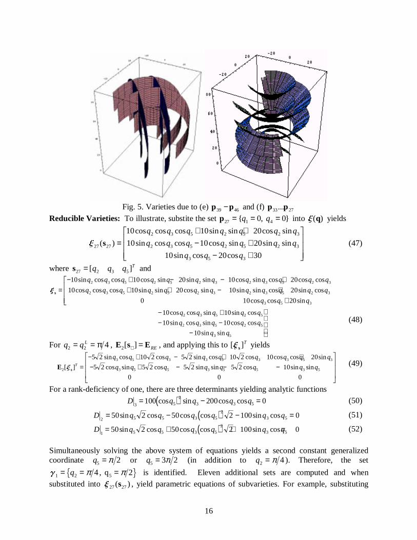
Fig. 5. Varieties due to (e) p p39 46− and (f) 2733...ppReducible Varieties: To illustrate, substite the set p27 1 40 0= = ={ , }q q into x( )q yields
x 27 27
2 3 5 2 5 2 3
2 3 5 2 5 2 3
3 5 3
10 10 20
10 10 20
10 20 30
( )
cos cos cos sin sin cos sin
sin cos cos cos sin sin sin
sin cos cos
s =+ +− +
− +
�
!
"
$###
q q q q q q q
q q q q q q q
q q q
(47)
where s27 2 3 5= [ ]q q q T and
x s =− + − − +
+ + − ++
�
!
10 10 20 10 20
10 10 20 10 20
0 10 20
2 3 5 2 5 2 3 2 3 5 2 3
2 3 5 2 5 2 3 2 3 5 2 3
3 5 3
sin cos cos cos sin sin sin cos sin cos cos cos
cos cos cos sin sin cos sin sin sin cos sin cos
cos cos sin
q q q q q q q q q q q q
q q q q q q q q q q q q
q q q
− +− −
−
10 10
10 10
10
2 3 5 2 5
2 3 5 2 5
3 5
cos cos sin sin cos
sin cos sin cos cos
sin sin
q q q q q
q q q q q
q q
(48)
For q q L2 2 4= = π , E s E2[ ]∈ = RE , and applying this to [ ]x s
T yields
E s2
3 5 3 3 5 3 3 5 3
3 5 5 3 5 5 3 5
5 2 10 2 5 2 10 2 10 20
5 2 5 2 5 2 5 2 10
0 0 0
[ ]
sin cos cos sin cos cos cos cos sin
cos sin cos sin sin cos sin sinxT
q q q q q q q q q
q q q q q q q q=− + − + +− + − − −
�
!
"
$###
(49)
For a rank-deficiency of one, there are three determinants yielding analytic functions
( )D q q q q3 5
2
3 3 5100 200 0= − =cos sin cos cos (50)
( )D q q q q q q2 5 5 3 5
2
3 550 2 50 2 100 0= − − =sin cos cos cos sin cos (51)
( )D q q q q q q1 5 5 3 5
2
3 550 2 50 2 100 0= + + =sin cos cos cos sin cos (52)
Simultaneously solving the above system of equations yields a second constant generalizedcoordinate q5 2= π or q5 3 2= π (in addition to q2 4= π ). Therefore, the set
g1 2 4 2= = =q π π, q5; @ is identified. Eleven additional sets are computed and when
substituted into x 27 27( )s , yield parametric equations of subvarieties. For example, substituting

17
g1 into Eq. (47) yields κ1 1 3 3 35 2 10 2 5 2 10 2 20 30( ) sin sin cosβ = + − + − +q q qT;
( ) ( )π π4 5 43≤ ≤q , where β1 3= q . Substituting all second-order singularity sets into Eq. (47)yields a number of curves κ j ; j = 1 12,..., , shown in Fig. 6a. The reducible variety whose
boundaries are now established and defined by segments is shown in Fig. 6b.
Fig. 6. (a) Subvarietis of x 27 shown as curves (b) The reducible variety x 27
The four reducible varieties due to ( ... )p p27 30 are shown in Fig. 7a. The manifold obtained bycombining all varieties is shown in Fig. 7b which represents the exact material removed.
Fig. 7 (a) Four reducible varieties (b) The boundary to the manifold (material removed)
7. EXAMPLE ON COMPUTING THE VOLUME

18
Consider a motion of the cutting tool characterized by a curve given by the parametric vector
G( ) cos sinu = 5 5 1u uT
. The curve will be rotated about three axes in space given by the
rotation matrices R i
i i i
i i i
v v v
v v v=−
−�
!
"
$###
cos . sin . sin
sin . cos . cos
. .
05 0866
05 0866
0 0866 05
i = 1 3,..., and the sweep vectors
Y1 1 13 3 1= cos sinv vT
, Y2 2 24 4 1= cos sinv vT
, and Y3 3 33 3 1= cos sinv vT
. This
operation is illustrated in Fig. 8.
x0
y0
z1
z2
z3z4
Γ(u)
v1v2
v3
Fig. 8 A four parameter verification
Every point in the manifold is characterized by the vector function
x( )
( ( . ) (. . . ) . .
( ( . ) ( . . . )
(. (. . ) ) (. . . (. . ) . ) )
q =− + − − + −
+ + − + −+ + + − + + −
�
!
−c c c c s s s c s c s s s s
c c s c c s c c c s s s
c c s c s c c c s s s
4 3 1 2 1 2 1 2 1 1 2 3 1 1 2
4 3 1 2 1 2 1 2 1 1 2 3
4 3 2 2 3 2 2 3 2 3 4
5 75 25 5 375 187
5 75 25 5
86 43 43 22 65 5 43 43 43
+ − − + − −+ − + + + − + − − +
+
"
$###
+
− +
. (. . . ) . . ( . )
( . . . . ( . . . ) . ( . ) )
5 75 25 5 56 5 5
375 187 56 5 75 25 5 5 5
0
3 1 2 1 1 2 1 2 1 2 1 2 3 4
1 1 2 1 2 3 1 1 2 1 2 2 1 1 2 3 4
c s c s c s s c c s s s s
c c c c c c c s s c s c s s s
where c1 denotes the Cosine of q1 and s1 denotes the Sine of q1 andv v v u3 2 1 = q q q q1 2 3 4 . For this 4-parameter NC operation, the varieties are
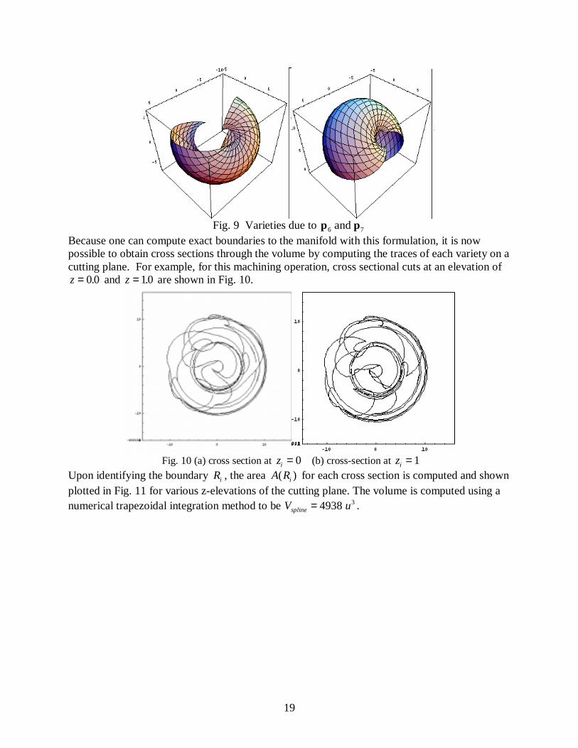
calculated by first determining the 22 singular sets. For example, the varietis atp6 3 42 3 2 3= = − = −q qπ π,; @ and p7 3 42 3 2 3= = =q qπ π,; @ are shown in Fig. 9.
19
Fig. 9 Varieties due to p p6 and 7
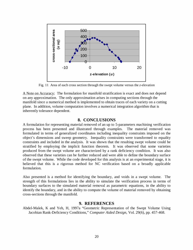
Because one can compute exact boundaries to the manifold with this formulation, it is nowpossible to obtain cross sections through the volume by computing the traces of each variety on acutting plane. For example, for this machining operation, cross sectional cuts at an elevation ofz = 0 0. and z = 10. are shown in Fig. 10.
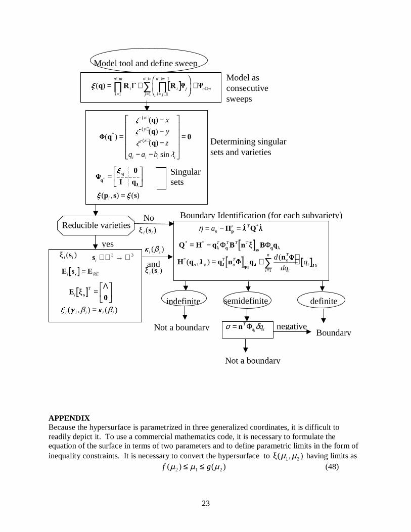
Fig. 10 (a) cross section at zi = 0 (b) cross-section at zi = 1Upon identifying the boundary Ri , the area A Ri( ) for each cross section is computed and shownplotted in Fig. 11 for various z-elevations of the cutting plane. The volume is computed using anumerical trapezoidal integration method to be V uspline = 4938 3 .
20
0
100
200
300
400
500
-10 0 10 20
z-elevation (u )
cro
ss-s
ecti
on
al a
rea
(u s
q)
Fig. 11 Area of each cross section through the swept volume versus the z-elevation
A Note on Accuracy: The formulation for manifold stratification is exact and does not dependon any approximation. The only approximation arises in computing sections through themanifold since a numerical method is implemented to obtain traces of each variety on a cuttingplane. In addition, volume computation involves a numerical integration algorithm that isinherently tolerance dependent.
8. CONCLUSIONSA formulation for representing material removed of an up to 5-parameters machining verificationprocess has been presented and illustrated through examples. The material removed wasformulated in terms of generalized coordinates including inequality constraints imposed on theobject’s dimensions and sweep geometry. Inequality constraints were transformed to equalityconstraints and included in the analysis. It was shown that the resulting swept volume could bestratified by employing the implicit function theorem. It was observed that some varietiesproduced from the swept volume are characterized by a rank deficiency condition. It was alsoobserved that these varieties can be further reduced and were able to define the boundary surfaceof the swept volume. While the code developed for this analysis is at an experimental stage, it isbelieved that this is a rigorous method for NC verification based on a broadly applicableformulation.
Also presented is a method for identifying the boundary, and voids in a swept volume. Thestrength of this formulations lies in the ability to simulate the verification process in terms ofboundary surfaces to the simulated material removal as parametric equations, in the ability toidentify the boundary, and in the ability to compute the volume of material removed by obtainingcross-sections through the manifold.
9. REFERENCESAbdel-Malek, K and Yeh, H, 1997a “Geometric Representation of the Swept Volume Using
Jacobian Rank-Deficiency Conditions,” Computer Aided Design, Vol. 29(6), pp. 457-468.

21
Abdel-Malek, K., Adkins, F., Yeh, H.J., and Haug, E.J., 1997, “On the Determination ofBoundaries to Manipulator Workspaces,” Robotics and Computer-Integrated Manufacturing,Vol. 13, No. 1, pp.63-72.
Abdel-Malek, K., and Yeh, H.J., 1997b, “Analytical Boundary of the Workspace for General 3-DOF Mechanisms, The International Journal of Robotics Research, Vol. 16, No. 2, pp.1-12.
Abdel-Malek, K., Yeh, H.J., and Othman, S., 1998, “Swept Volumes, Void and BoundaryIdentification”, Computer Aided Design, Vol. 30, No. 13, pp. 1009-1018.
Ahn, JC, Kim, MS, Lim, SB, 1997, "Approximate general sweep boundary of 2D curved object",CVGIP: Computer Vision Graphics and Image Processing, Vol. 55, pp. 98-128.
Blackmore, D, Leu, MC, Wang, LP, Jiang, H, 1997, “Swept Volumes: a retrospective andprospective view,” Neural parallel and Scientific Computations, Vol. 5, pp. 81-102.
Blackmore, D., Leu, M.C., Wang, L.P., 1997, “Sweep-envelope differential equation algorithmand its application to NC machining verification”, Computer Aided Design Vol. 29, No. 9,pp. 629-637.
Blackmore, D, Leu, MC, Wang, LP, and Jiang, H, 1997, “Swept Volumes: a Retrospective andProspective View,” Neural, Parallel, and Scientific Computations, 5, pp. 81-102.
Boussac, S and Crosnier, A, 1996, “Swept volumes generated from deformable objectsapplication to NC verification”, Proceedings of the 13th IEEE International Conference onRobotics and Automation. Part 2 (of 4) Apr 22-28, Vol. 2, Minneapolis, MN, pp. 1813-1818
Elber, G, 1997, “Global error bounds and amelioration of sweep surfaces,” Computer AidedDesign, Vol. 29, pp.441-447.
Farin, G., 1993, Curves and Surfaces for Computer Aided Geometric Design, Academic Press,San Diego, CA.
Guillemin, V. and Pollack, A., 1974, Differential Topology, Prentice-Hall.Jerard, R and Drysdale, R 1991, Methods for geometric modeling, simulation, and spatial
verification of NC machining programs”, Product Modeling for Computer Aided Design,North Holland, Amsterdam, pp. 1-14.
Jerard, R and Drysdale, R, 1988 ‘Geometric Simulation of Numerical Control Machinery’ ASMEComputers Engineer Vol 2, pp129-136.
Koren, Y. and Lin, R.S., 1995, “Five-axis surface interpolators, Annals of CIRP, 44(1), 379-382.Leu, M C., Wang, L, Blackmore, D., 1997, “Verification program for 5-axis NC machining with
general APT tools” CIRP Annals - Manufacturing Technology Vol. 46, No. 1, pp. 419-424Liang, X, Xiao, T, Han, X, Ruan, JX, 1997, Simulation Software GNCV of NC Verification,
Author Affiliation: ICIPS Proceedings of the 1997 IEEE International Conference onIntelligent Processing Systems, Part 2 Oct 28-31, Vol. 2, Beijing, China pp. 1852-1856.
Ling, ZK and Chase, T 1996, “Generating the swept area of a body undergoing planar motion,”ASME J. Mech. Design, Vol 118, pp221-233.
Liu, C, and Esterling, D, 1997, “Solid Modeling of 4-Axis Wire EDM Cut Geometry”,Computer Aided Design Vol. 29, No. 12, pp. 803-810
Liu, C., Esterling, D.M., Fontdecaba, J., Mosel, E, 1996, “Dimensional verification of NCmachining profiles using extended quadtrees”, Computer Aided Design Vol. 28, No. 11, pp.845-852.
Liu, Chonglin; Esterling, Donald, 1997, “Solid modeling of 4-axis wire EDM cut geometry”,Computer Aided Design v 29 n 12, pp803-810.
Lu, Y.C. “Singularity Theory and an Introduction to Catastrophe Theory”, Springer-Verlag, NewYork, 1976

22
Menon, J.P. and Robinson, D.M. 1993, “Advanced NC verification via massively parallelraycasting, “ ASME manufacturing Review, Vol. 6, 141-154.
Menon, J.P., Voelcker, H.B. 1992, “Toward a comprehensive formulation of NC verification as amathematical and computational problem”, Proceedings of the 1992 Winter Annual Meetingof ASME, Nov 8-13, Vol. 59, Anaheim, CA, pp. 147-164.
Narvekar, AP, Huang, Y, and Oliver, J, 1992, “Intersection of rays with parametric envelopesurfaces representing five-axis NC milling tool swept volumes”, Proceedings of the 199218th Annual ASME Design Automation Conference, Vol. 44, Scottsdale, AZ, pp. 223-230.
Oliver, J and Goodman, E, 1990, “Direct Dimensional NC Verification” Computer Aided DesignVol. 22, pp. 3-9.
Oliver, J H ‘Efficient Intersection of Surface Normals with Milling Tool Swept Volumes forDiscrete Three-axis NC Verification’ ASME DE Vol 23(1) (1990) pp159-164.
Sourin, A and Pasko, A 1996, “A function represenatation for sweeping by a moving solid,”IEEE Transactions on visualization and Computer Graphics, Vol2, pp11-18.
Spivak, M. 1968, Calculus on Manifolds, Benjamin/Cummeings.Takata, S, Tsai, MD, and Inui, M, “1992, “A cutting simulation system for machinability
evaluation using a workpiece model,” Annals of CIRP 38:539-542.Voelker, H B and Hunt, W A, 1985, ‘The Role of Solid Modeling in Machining Process
Modeling and NC Verification’ SAE Tech. Paper #810195.Wang, W P and Wang, K.K., 1986, “Geometric Modeling for Swept Volume of Moving Solids”
IEEE Computer Graphics and Applications, Vol. 6, No. 12, pp. 8-17.
10. Appendix A
23
Reducible varietiesNo
yes
Boundary Identification (for each subvariety)
Determining singularsets and varieties
Model asconsecutivesweeps
ξ i i( )s
ξ i i( )s si ∈ℜ → ℜ3 3
E0si
TξΛ
=�!
"$#
k i i( )β
ξ i i( )sand
Q H q B n B qq ss q* = − Φ ξ Φ∗
λ λT T T T
indefinite
Not a boundary
semidefinite
σ δ= nTq ii
qΦ
Not a boundary
negativeBoundary
definite
Model tool and define sweep
x G Y Y( )q R R= +���
��� +
=
+
= +
+ −
=
+
+∏ ∏∑ii
n m
ii j
n m
jj
n m
n m1 1
1
1
F( )
( )
( )
( )
sin
*q
q
q
q0=
−−−
− −
�
!
"
$
####=
x
x
x
l
( )
( )
( )
x
y
z
i i i i
x
y
z
q a b
Fx
l
q
q 0
I q* =
�!
"$#
Singularsets
x x( , ) ( )p s si =
E s Ei REe=
x g ki i i i i( , ) ( )β β=
η = − ′ =anTII Qp
& &
*l l
H q q n qn
*( , )(
o oT
oT o
T
ii
i
n d
dqql F
F
l l ll= + ⋅
=∑ )
1
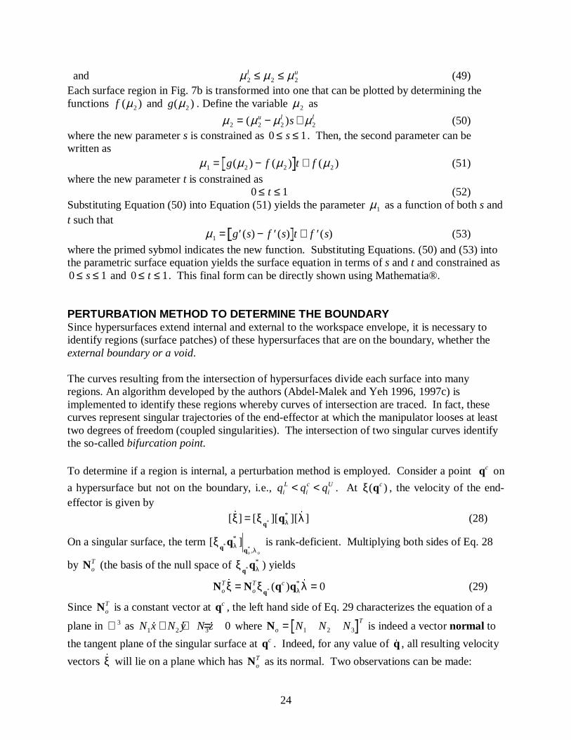
APPENDIXBecause the hypersurface is parametrized in three generalized coordinates, it is difficult toreadily depict it. To use a commercial mathematics code, it is necessary to formulate theequation of the surface in terms of two parameters and to define parametric limits in the form ofinequality constraints. It is necessary to convert the hypersurface to ξ( , )µ µ1 2 having limits as
f g( ) ( )µ µ µ2 1 2≤ ≤ (48)
24
and µ µ µ2 2 2l u≤ ≤ (49)
Each surface region in Fig. 7b is transformed into one that can be plotted by determining thefunctions f ( )µ2 and g( )µ2 . Define the variable µ 2 as
µ µ µ µ2 2 2 2= − +( )u l ls (50)where the new parameter s is constrained as 0 1≤ ≤s . Then, the second parameter can bewritten as
µ µ µ µ1 2 2 2= − +g f t f( ) ( ) ( ) (51)
where the new parameter t is constrained as0 1≤ ≤t (52)
Substituting Equation (50) into Equation (51) yields the parameter µ1 as a function of both s andt such that
µ1 = ′ − ′ + ′g s f s t f s( ) ( ) ( ) (53)
where the primed sybmol indicates the new function. Substituting Equations. (50) and (53) intothe parametric surface equation yields the surface equation in terms of s and t and constrained as0 1≤ ≤s and 0 1≤ ≤t . This final form can be directly shown using Mathematia®.
PERTURBATION METHOD TO DETERMINE THE BOUNDARYSince hypersurfaces extend internal and external to the workspace envelope, it is necessary toidentify regions (surface patches) of these hypersurfaces that are on the boundary, whether theexternal boundary or a void.
The curves resulting from the intersection of hypersurfaces divide each surface into manyregions. An algorithm developed by the authors (Abdel-Malek and Yeh 1996, 1997c) isimplemented to identify these regions whereby curves of intersection are traced. In fact, thesecurves represent singular trajectories of the end-effector at which the manipulator looses at leasttwo degrees of freedom (coupled singularities). The intersection of two singular curves identifythe so-called bifurcation point.
To determine if a region is internal, a perturbation method is employed. Consider a point qc on
a hypersurface but not on the boundary, i.e., q q qiL
ic
iU< < . At ξ( )qc , the velocity of the end-
effector is given by
[ & ] [ ][ ][ & ]**ξ λλ= ξ
qq (28)
On a singular surface, the term [ ]**
*
,ξ
q qqλ
λo o
is rank-deficient. Multiplying both sides of Eq. 28
by NoT (the basis of the null space of ξ
qq*
*λ ) yields
N N q qqo
ToT c
& ( ) &
**ξ λλ= =ξ 0 (29)
Since NoT is a constant vector at qc , the left hand side of Eq. 29 characterizes the equation of a
plane in ℜ3 as N x N y N z1 2 3 0& & &+ + = where No
TN N N= 1 2 3 is indeed a vector normal to
the tangent plane of the singular surface at qc . Indeed, for any value of &q , all resulting velocity
vectors &ξ will lie on a plane which has NoT as its normal. Two observations can be made:
25
(i) The basis of the null space of ξq
q**λ
T
is the vector normal to the singular surface at qc .
(ii) For any given joint velocity vector &q , the velocity of the end-effector is either tangent to thesingular surface or zero, i.e., the normal component of the end-effector velocity is always
zero, i.e., vn o oT= ⋅ = =N N& &ξ ξ 0 (this result is reported by Haug et al. 1996 using a different
approach).For this normal, two points along the normal on each side of the surface can be found as
ξ ξp c1 2, ( )= ±q N∂ϑ (30)
where ∂ϑ is a small variation from ξ( )qc (e.g., ∂ϑ = 01. ). If both points ξ p1 and ξ p2 satisfy the
constraint equation, then the region for which ξ( )qc belongs is internal to the boundary.Performing this test on all regions yields boundary surface patches defined by the equations ofξ( )*q and bound by the numerical curves.
Φq s q sq
o o,
NC verification software based on ray casting methods were demonstrated by (Liang, et al.1997).