near-surface hydrologic response for a steep, unchanneled

NEAR-SURFACE HYDROLOGIC RESPONSE FOR A STEEP,UNCHANNELED CATCHMENT NEAR COOS BAY, OREGON:

1. SPRINKLING EXPERIMENTS

BRIAN A. EBEL*†, KEITH LOAGUE*, WILLIAM E. DIETRICH**,DAVID R. MONTGOMERY***, RAYMOND TORRES§, SUZANNE P. ANDERSON§§,

and THOMAS W. GIAMBELLUCA‡

ABSTRACT. Sprinkling systems are frequently used to simulate rainfall for process-based investigations of near-surface hydrologic response without measuring or account-ing for spatial variability. Data analyses from three sprinkling experiments at the CoosBay 1 experimental catchment (CB1) demonstrate considerable spatial variability insprinkling. Furthermore, simulated rainfall from sprinklers was found to be moreheterogeneous than natural storms at CB1. Water balance calculations and evapotrans-piration estimates indicate that evaporation of airborne droplets is a significantportion of applied sprinkling rates, although still less than the amount blown off thefield site by strong winds. Incorporation of spatial variability in sprinkling input andsoil-water storage did not significantly change water balance calculations. Saturationpatterns within the near-surface soil profile and the timing of tensiometric responseare affected by sprinkling heterogeneity. Pore-water pressure and saturation develop-ment at the soil-saprolite interface are primarily controlled by convergent surface /subsurface topography and bedrock fracture flow, but are also sensitive to sprinklingspatial variations. The analyses presented herein suggest that incorporating spatialvariability in sprinkling rates is important when conducting hydrologic-response model-ing of sprinkler experiments. This paper is the first-part of a two-part series focused onCB1. The data analyses in this paper are used to parameterize comprehensivephysics-based hydrologic-response simulations of three CB1 sprinkling experimentsreported in the companion paper.

introductionLandscape evolution, while driven by diverse physical, chemical, and biological

processes, is often largely controlled by the actions of water on the surface and withinthe subsurface (Gilbert, 1877). With this in mind, the importance of near-surfacehydrologic-response should not be underestimated when investigating geomorphicprocesses. At the same time, the spatial heterogeneity present in natural systems (forexample, saturated hydraulic conductivity, soil / bedrock thickness, and topography)combined with temporal variations in precipitation intensity and duration make itdifficult to quantitatively evaluate the relative influence of the different factorsgoverning hydrologic processes. Using sprinkling systems to mimic precipitationfacilitates controlling the temporal variations in rainfall, simplifying hydrologic-response analysis. The strong link between geomorphic and hydrologic processesmotivated the controlled sprinkling experiments at the Coos Bay experimental catch-ment (CB1). The primary objectives of the CB1 study were to investigate the mecha-nisms responsible for pore-water pressure development and shallow subsurface runoffgeneration. Elevated pore-water pressures can reduce effective stresses, driving slopefailure. It is worth noting that CB1 failed as a landslide in 1996 in response to a large

*Department of Geological and Environmental Sciences, Stanford University, Stanford, California94305-2115

**Department of Earth and Planetary Science, University of California, Berkeley, California 94720-4767***Department of Earth and Space Sciences, University of Washington, Seattle, Washington 98195§Department of Geological Sciences, University of South Carolina, Columbia, South Carolina 29208§§Institute of Arctic and Alpine Research, University of Colorado, Boulder, Colorado 80309-0450‡Department of Geography, University of Hawaii at Manoa, Honolulu, Hawaii 96822† Corresponding author: [email protected]

[American Journal of Science, Vol. 307, April, 2007, P. 678–708, DOI 10.2475/04.2007.02]

678

storm (Montgomery and others, manuscript in preparation). To the best of theauthors’ knowledge, the CB1 measurements represent the most complete hydrologic-response data set available for any catchment that has failed.

The sprinkling experiments and long-term monitoring effort at CB1 (Montgom-ery, ms, 1991; Anderson, ms, 1995; Torres, ms, 1997) focused on producing acomprehensive dataset pertaining to hydrologic response. The published work fromCB1 (Anderson and others, 1997a, 1997b, 2002; Montgomery and others, 1997, 2002;Torres and others, 1998; Anderson and Dietrich, 2001; Montgomery and Dietrich,2002) has contributed to understanding the mechanisms of pore-water pressuredevelopment, subsurface runoff generation, and weathering in unchanneled valleys.This paper is the first of a two-part series focused on the CB1 catchment. The workreported herein evaluates the spatial variability in sprinkling and the observed effectson the CB1 hydrologic response. In the companion paper (Ebel and others, 2007), thehydrologic response from the three CB1 sprinkling experiments is simulated with acomprehensive physics-based model to better understand runoff and pore-waterpressure generation. The data analyses and conclusions reported here provide boththe foundation and the evaluation framework for the numerical modeling in thesecond paper.

cb1 study areaField-scale experiments designed to investigate hydrologically-driven landscape

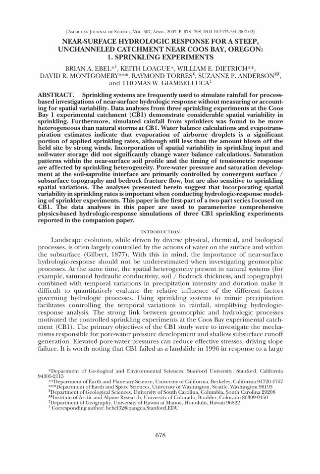
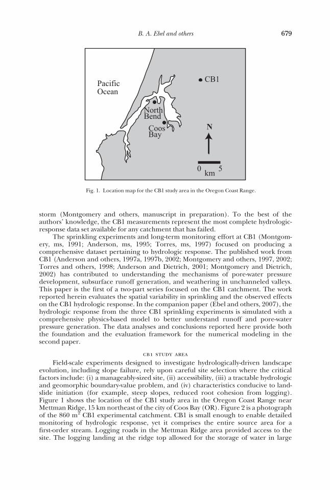
evolution, including slope failure, rely upon careful site selection where the criticalfactors include: (i) a manageably-sized site, (ii) accessibility, (iii) a tractable hydrologicand geomorphic boundary-value problem, and (iv) characteristics conducive to land-slide initiation (for example, steep slopes, reduced root cohesion from logging).Figure 1 shows the location of the CB1 study area in the Oregon Coast Range nearMettman Ridge, 15 km northeast of the city of Coos Bay (OR). Figure 2 is a photographof the 860 m2 CB1 experimental catchment. CB1 is small enough to enable detailedmonitoring of hydrologic response, yet it comprises the entire source area for afirst-order stream. Logging roads in the Mettman Ridge area provided access to thesite. The logging landing at the ridge top allowed for the storage of water in large

Fig. 1. Location map for the CB1 study area in the Oregon Coast Range.

679B. A. Ebel and others 679

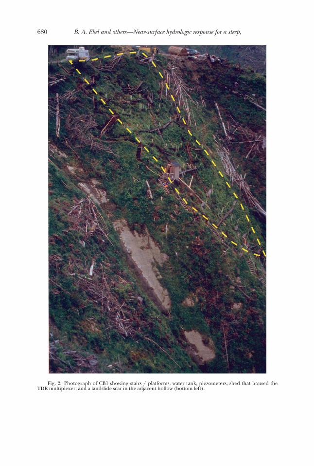
Fig. 2. Photograph of CB1 showing stairs / platforms, water tank, piezometers, shed that housed theTDR multiplexer, and a landslide scar in the adjacent hollow (bottom left).

680 B. A. Ebel and others—Near-surface hydrologic response for a steep,

holding tanks that facilitated using the topographic relief to drive sprinklers thatmimic rainfall. Figure 3A shows a contour map of the steep (�43° slope) surfacetopography and surface topography hollow axis at CB1 based on the detailed theod-alite survey from Montgomery and others (1997). Figure 3B shows a contour map ofthe soil-saprolite interface topography and soil-saprolite interface hollow axis based onover 100 measurements from piezometer installation (Montgomery and others, 1997;Schmidt, ms, 1999). The mean annual rainfall at the nearby North Bend (OR) airport,based on 29 years of data, is �1.6 m yr-1 (Taylor and others, 2005). The old growthconiferous forest at CB1 was removed by a fire �100 years ago. The second growthforest was logged by clear-cutting methods in February and March, 1987, treated withan application of a broadleaf herbicide (Roundup®) in July, 1988 (Torres, ms, 1997)to remove groundcover, and replanted with Douglas Fir (Pseudotsuga menziesii) seed-lings in January, 1989 (Montgomery, ms, 1991). The broadleaf vegetation [Alder(Alnus) trees and blackberry (Rubus) vines] was periodically trimmed at the site from1990 through 1992; the vegetation was not cut after 1992. The current state ofvegetation at the site consists of Douglas Fir (Pseudotsuga menziesii) trees from 5 to 8meters in height (see picture in Ebel and Loague, 2006) with undergrowth consisting

Fig. 3. (A) Contour map of the surface topography showing the surface hollow axis and the woodenplatform network used to install and monitor the CB1 instrumentation. (B) Contour map of the CB1 soildepth and the hollow axis of the soil-saprolite interface.

681unchanneled catchment near Coos Bay, Oregon: 1. Sprinkling experiments

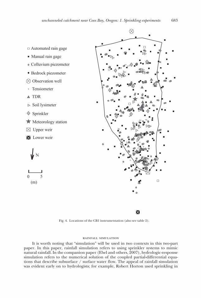
of Alder (Alnus), sword fern (Polystichum munitum), and bramble (Rubus). Table 1summarizes the three sprinkling and tracer experiments conducted at CB1. Figure 4 isa map of the CB1 instrumentation that facilitates a detailed characterization ofhydrologic-response (Anderson and others, 1997b; Montgomery and others, 1997;Torres and others, 1998). Thirteen rotating Rainbird® sprinklers (fig. 4) mounted 2 mabove the ground were regulated using a system of pressure valves and gauges adjustedto maintain the flow rates. A 38,000 L storage tank for experiment 3 (15,000 L inexperiments 1 and 2) located at the ridge crest (fig. 2) supplied water to the sprinklersthrough a pipe network. The tank was refilled using a 4,000 L tanker truck thattransported water from a quarry pond 2 km away. The experiment 1 and 3 intendedirrigation rates (table 1) represent �1 year 24 hour recurrence interval storms. Theexperiment 2 irrigation rate (table 1) represents a 1 to 2 year 24 hour recurrenceinterval storm. Both recurrence intervals are based on the North Bend and Alleghany(OR) rainfall records spanning, respectively, 23 and 41 years (Montgomery and others,1997).

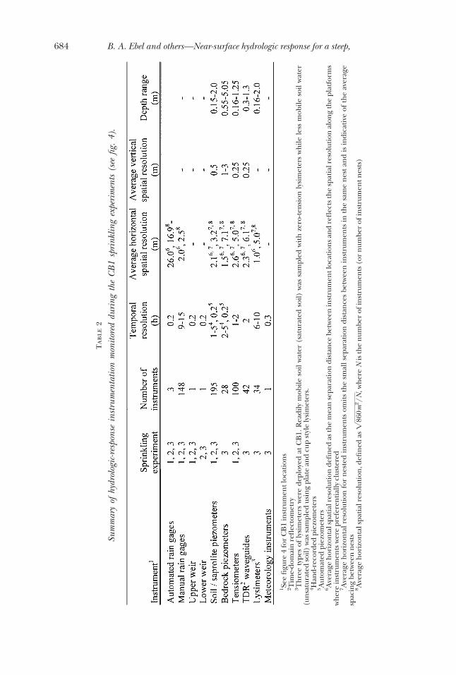
Table 2 provides information on the spatial and temporal distribution of thehydrologic-response observations collected during the three sprinkling experiments(table 1). These observations (see table 2, fig. 4) were made at 148 manual rain gages,three automated tipping-bucket rain gages, 223 piezometers, 100 tensiometers, 42time-domain reflectometry (TDR) waveguide pairs, and 34 lysimeters (Anderson andothers, 1997a, 1997b; Montgomery and others, 1997; Torres and others, 1998). Figure3A shows the suspended wooden platforms that the instrumentation in figure 4 wasemplaced and monitored from. Seepage from subsurface flow at CB1 was monitored attwo v-notch weirs equipped with stage-height recorders. The upper weir is located atthe channel head and anchored to bedrock; plastic coated plywood sealed into thebedrock routes soil water into the flume. The lower weir, located approximately 15 mdownslope from the upper weir, was installed during experiment 2 to capture thebedrock component of near-surface flow that was missing in the water balance fromexperiment 1. The upper weir recorded from January 1990 through November 1996;the lower weir recorded from October 1991 through November 1996.

Relative to the information necessary for investigating hydrologic-response viaphysics-based simulation (Ebel and others, 2007), the CB1 measurements providetopography, characteristics of the soil [thickness, saturated hydraulic conductivity(slug tests), soil-water content and porosity (TDR measurements), capillary pressurerelationships (from plot experiments)], irrigation rates, meteorology data (collectedfrom net radiometers, soil heat flux plates, anemometers, thermometers, and relativehumidity sensors), discharge at the weirs, pressure head response in the near surface,tracer concentrations (from ceramic cup lysimeters, tension lysimeters, and platelysimeters), and discharge chemistry.

Table 1

Summary of CB1 sprinkling experiments (after table 2 from Anderson and others, 1997b)


rainfall simulation

It is worth noting that “simulation” will be used in two contexts in this two-partpaper. In this paper, rainfall simulation refers to using sprinkler systems to mimicnatural rainfall. In the companion paper (Ebel and others, 2007), hydrologic-responsesimulation refers to the numerical solution of the coupled partial-differential equa-tions that describe subsurface / surface water flow. The appeal of rainfall simulationwas evident early on to hydrologists; for example, Robert Horton used sprinkling in

Fig. 4. Locations of the CB1 instrumentation (also see table 2).


Tab

le2

Sum

mar

yof

hydr

olog

ic-re

spon

sein

stru

men

tatio

nm

onito

red

duri

ngth

eC

B1

spri

nklin

gex

peri

men

ts(s

eefig

.4)

.

1Se

efi

gure

4fo

rC

B1

inst

rum

entl

ocat

ion

s2T

ime-

dom

ain

refl

ecto

met

ry3T

hre

ety

pes

ofly

sim

eter

sw

ere

depl

oyed

atC

B1.

Rea

dily

mob

ileso

ilw

ater

(sat

urat

edso

il)w

assa

mpl

edw

ith

zero

-ten

sion

lysi

met

ers

wh

ilele

ssm

obile

soil

wat

er(u

nsa

tura

ted

soil)

was

sam

pled

usin

gpl

ate

and

cup

styl

ely

sim

eter

s.4H

and-

reco

rded

piez

omet

ers

5A

utom

ated

piez

omet

ers

6A

vera

geh

oriz

onta

lspa

tial

reso

luti

onde

fin

edas

the

mea

nse

para

tion

dist

ance

betw

een

inst

rum

entl

ocat

ion

san

dre

flec

tsth

esp

atia

lres

olut

ion

alon

gth

epl

atfo

rms

wh

ere

inst

rum

ents

wer

epr

efer

enti

ally

clus

tere

d7A

vera

geh

oriz

onta

lres

olut

ion

for

nes

ted

inst

rum

ents

omit

sth

esm

alls

epar

atio

ndi

stan

ces

betw

een

inst

rum

ents

inth

esa

me

nes

tan

dis

indi

cati

veof

the

aver

age

spac

ing

betw

een

nes

ts8A

vera

geh

oriz

onta

lspa

tial

reso

luti

on,d

efin

edas

�86

0m2/N

,wh

ere

Nis

the

num

ber

ofin

stru

men

ts(o

rn

umbe

rof

inst

rum

entn

ests

)


1914 to examine infiltration capacities (Wisler and Brater, 1959). A review of rainfallsimulation studies from 1914 to 1969 is provided by Hall (1970). More recently, rainfallsimulators have been employed in studies of hydrologic response (for example,Hornberger and others, 1991; Waddington and Devito, 2001; Sharpley and Kleinman,2003) and erosion (for example, Parsons and others, 1998; Wilson, 1999; Motha andothers, 2002). The advantages of controlling the sprinkling intensity and duration (aswell as the solute input), to minimize temporal variability, do not come without thedifficulties of reproducing natural rainfall characteristics (that is, spatially-uniformintensities, drop size distributions, and drop kinetic energies). Almost all rainfallsimulator studies forgo rigorous analysis of the spatial variations in rainfall intensity(Lascelles and others, 2000). The effort reported herein compares spatial variations inintensity between simulated and natural storms and evaluates the effects of sprinklingheterogeneity on the observed CB1 hydrologic response.

Common Metrics of Rainfall Simulator PerformanceCommon metrics for evaluating the spatial uniformity of sprinkling include the

coefficient of uniformity (CU), the coefficient of variation (CV), and the standarddeviation (SD). The CU (Christiansen, 1942) is calculated, as a percentage, by:

CU � 100�1 �¥N �Di � �D�

¥N Di� (1)

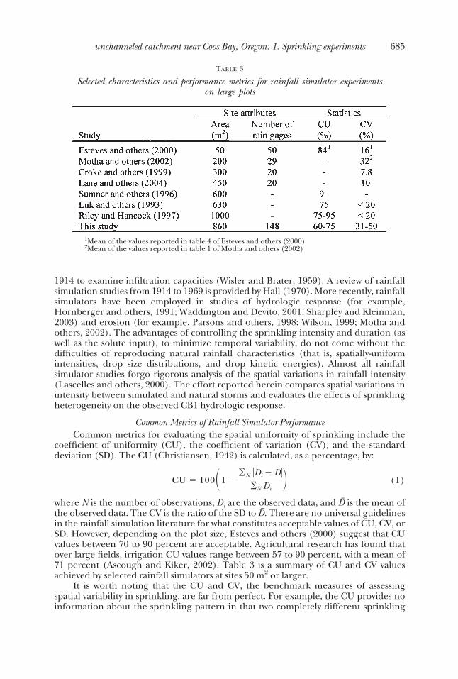
where N is the number of observations, Di are the observed data, and �D is the mean ofthe observed data. The CV is the ratio of the SD to �D. There are no universal guidelinesin the rainfall simulation literature for what constitutes acceptable values of CU, CV, orSD. However, depending on the plot size, Esteves and others (2000) suggest that CUvalues between 70 to 90 percent are acceptable. Agricultural research has found thatover large fields, irrigation CU values range between 57 to 90 percent, with a mean of71 percent (Ascough and Kiker, 2002). Table 3 is a summary of CU and CV valuesachieved by selected rainfall simulators at sites 50 m2 or larger.

It is worth noting that the CU and CV, the benchmark measures of assessingspatial variability in sprinkling, are far from perfect. For example, the CU provides noinformation about the sprinkling pattern in that two completely different sprinkling

Table 3

Selected characteristics and performance metrics for rainfall simulator experimentson large plots

1Mean of the values reported in table 4 of Esteves and others (2000)2Mean of the values reported in table 1 of Motha and others (2002)


patterns can result in the same CU. Esteves and others (2000) compared CU and CVvalues with contour maps of intensity and found appreciable spatial variability, despitehigh values of CU and low values of CV (see table 3). Lascelles and others (2000) alsoused contour maps of sprinkling intensity to illustrate considerable spatial andtemporal variability, despite CU values consistently greater than 70 percent.

Sprinkling Variability at CB1The CB1 dataset is ideal for (i) assessing the spatial variations in irrigation

intensity / depth, (ii) comparing the sprinkling variability with natural rain variability,and (iii) determining the effects of spatial variability in sprinkling intensity onnear-surface hydrologic response. High spatial resolution characterization of the threeCB1 sprinkling experiments is facilitated by the 148 wedge rain gages (fig. 4) that weremonitored twice daily (�9:00 am and �6:00 pm). Three automated tipping-bucketrain gages (fig. 4) recorded sprinkling rates every 10 minutes. Rates of sprinkling arecalculated as the depths recorded in the manual gages divided by the time betweengage readings. For this study, it is assumed that all rain gage levels were read at thesame time. Given that it took 30 to 45 minutes to read all the gages and the time inbetween readings was greater than 10 hours, this assumption has a small effect on theaccuracy of the observed rates.

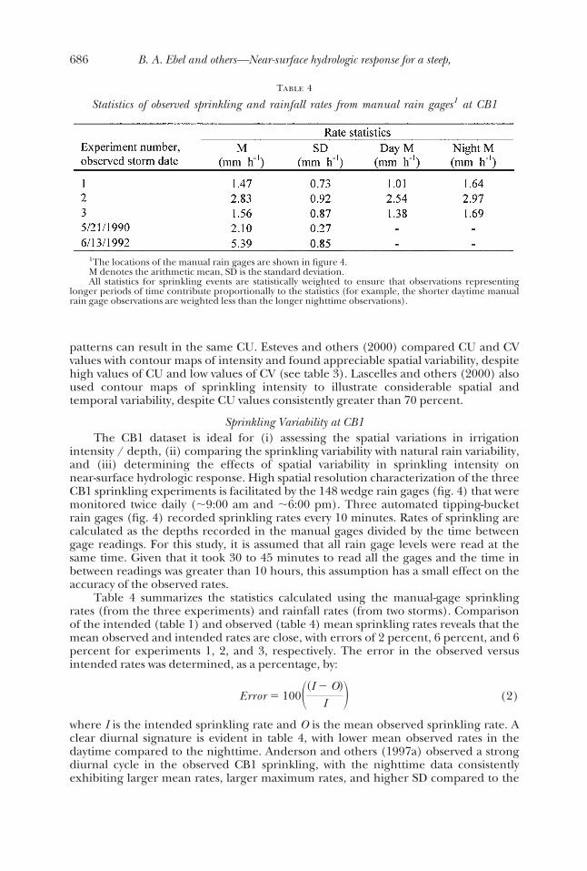
Table 4 summarizes the statistics calculated using the manual-gage sprinklingrates (from the three experiments) and rainfall rates (from two storms). Comparisonof the intended (table 1) and observed (table 4) mean sprinkling rates reveals that themean observed and intended rates are close, with errors of 2 percent, 6 percent, and 6percent for experiments 1, 2, and 3, respectively. The error in the observed versusintended rates was determined, as a percentage, by:

Error � 100��I � O�

I � (2)

where I is the intended sprinkling rate and O is the mean observed sprinkling rate. Aclear diurnal signature is evident in table 4, with lower mean observed rates in thedaytime compared to the nighttime. Anderson and others (1997a) observed a strongdiurnal cycle in the observed CB1 sprinkling, with the nighttime data consistentlyexhibiting larger mean rates, larger maximum rates, and higher SD compared to the

Table 4

Statistics of observed sprinkling and rainfall rates from manual rain gages1 at CB1

1The locations of the manual rain gages are shown in figure 4.M denotes the arithmetic mean, SD is the standard deviation.All statistics for sprinkling events are statistically weighted to ensure that observations representing

longer periods of time contribute proportionally to the statistics (for example, the shorter daytime manualrain gage observations are weighted less than the longer nighttime observations).


daytime sprinkling rates. It is worth noting that a higher SD does not necessarilydenote more spatially variable rainfall because the SD for similarly shaped distributionswill be larger for the higher rate. A better characterization of the diurnal variability isprovided by the CV and / or the CU. Table 5 summarizes the CU and CV values fromthe three sprinkling experiments and two natural storms. Perusal of table 5 illustratesthat despite considerable differences in the diurnal mean sprinkling rate, there is littlediurnal variation in the CV or the CU, indicating that the overall spatial variabilitychanges little in response to diurnal factors.

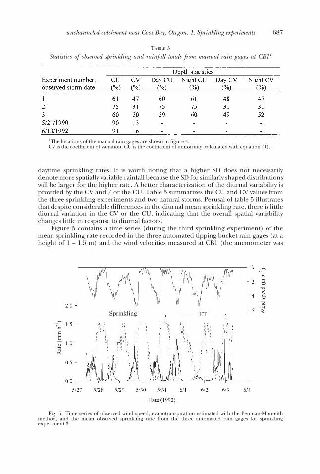
Figure 5 contains a time series (during the third sprinkling experiment) of themean sprinkling rate recorded in the three automated tipping-bucket rain gages (at aheight of 1 – 1.5 m) and the wind velocities measured at CB1 (the anemometer was

Table 5

Statistics of observed sprinkling and rainfall totals from manual rain gages at CB11

1The locations of the manual rain gages are shown in figure 4.CV is the coefficient of variation; CU is the coefficient of uniformity, calculated with equation (1).

Fig. 5. Time series of observed wind speed, evapotranspiration estimated with the Penman-Monteithmethod, and the mean observed sprinkling rate from the three automated rain gages for sprinklingexperiment 3.


positioned at a height of 3.0 m). The sprinklers are positioned at a height of 2.0 m.While the automated rain gages capture the overall temporal trends of sprinkling rates(fig. 5), the rates of sprinkling are inaccurate, with observed sprinkling rates approach-ing zero and total depths less than detected in nearby manual gages. Torres (ms, 1997)attributed the error in the automated gauge rates to the elevated gage heights (1 –1.5 m), relative to the manual rain gages that are positioned 0.15 to 0.4 m aboveground level. Rodda and Smith (1986) and Newson and Clarke (1976) found thatelevated rain gages may result in undercatch because of droplet trajectories, with theundercatch enhanced by wind. Comparison of the wind speed and automated gagesprinkling rate time series (see fig. 5) suggests that wind enhances undercatch at theCB1 automated rain gages during the sprinkling experiments, which was also notedfrom observations during the sprinkling experiments (see Montgomery, ms, 1991;Torres, ms, 1997).

The CB1 values of CU and CV (shown in table 5) are equivalent (75% forexperiment 2) to slightly less uniform (61 and 60%, for experiments 1 and 3,respectively) than those of Luk and others (1993) and Riley and Hancock (1997) forsimilarly sized areas (table 3). It is worth noting the steep terrain of CB1 (fig. 3A)makes uniform sprinkling difficult because of large head differences in the sprinklerlines. The CU and CV values in table 5 also indicate that higher sprinkling ratesresulted in a more uniform (higher CU and lower CV) spatial distribution of sprinklingdepths. The spatial uniformity decreases with increasing sprinkling rate for mostrainfall simulators (for example, Esteves and others, 2000), or does not vary at all(Loch and others, 2001). The increase of uniformity with sprinkling rate at CB1 likelyreflects a decline in pressure at the sprinkler nozzle with increasing sprinkling rate.Lower nozzle pressures produce fewer fine droplets and mist (Kincaid, 1996; Tarjueloand others, 2000), resulting in less wind-driven alteration of the sprinkling pattern.

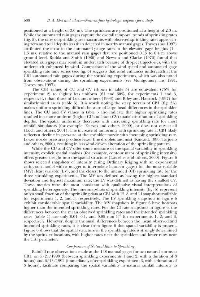
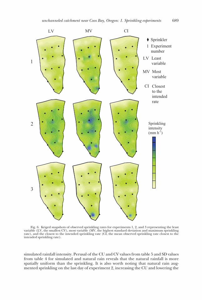
While the CU and CV offer some measure of the spatial variability in sprinklingintensity, explicit spatial analysis (for example, contour maps of sprinkling intensity)offers greater insight into the spatial structure (Lascelles and others, 2000). Figure 6shows selected snapshots of intensity (using Ordinary Kriging with an exponentialvariogram model with a nugget to interpolate between gages) for the most variable(MV), least variable (LV), and the closest to the intended (CI) sprinkling rate for thethree sprinkling experiments. The MV was defined as having the highest standarddeviation and highest maximum rate; the LV was defined as having the smallest CV.These metrics were the most consistent with qualitative visual interpretations ofsprinkling heterogeneity. The nine snapshots of sprinkling intensity (fig. 6) representonly a small fraction of the sprinkling data at CB1 with 12, 8, and 14 snapshots availablefor experiments 1, 2, and 3, respectively. The LV sprinkling snapshots in figure 6exhibit considerable spatial variability. The MV snapshots in figure 6 have hotspotshigher than the intended sprinkling rates. For the CI rate snapshots in figure 6, thedifferences between the mean observed sprinkling rates and the intended sprinklingrates (table 1) are only 0.01, 0.1, and 0.05 mm h-1 for experiments 1, 2, and 3,respectively. However, despite the small differences between the mean observed andintended sprinkling rates, it is clear from figure 6 that spatial variability is present.Figure 6 shows that the spatial structure in the sprinkling rates is strongly determinedby the sprinkler locations, with higher rates near the sprinklers and lower rates nearthe CB1 perimeter.

Comparison of Natural Rain to SprinklingRainfall rate observations made at the 148 manual gages for two natural storms at

CB1, on 5/21/1990 (between sprinkling experiments 1 and 2, with a duration of 8hours) and 6/13/1992 (immediately after sprinkling experiment 3, with a duration of3 hours), facilitate comparing the spatial variability in natural rainfall intensity to


simulated rainfall intensity. Perusal of the CU and CV values from table 5 and SD valuesfrom table 4 for simulated and natural rain reveals that the natural rainfall is morespatially uniform than the sprinkling. It is also worth noting that natural rain aug-mented sprinkling on the last day of experiment 2, increasing the CU and lowering the

Fig. 6. Kriged snapshots of observed sprinkling rates for experiments 1, 2, and 3 representing the leastvariable (LV, the smallest CV), most variable (MV, the highest standard deviation and maximum sprinklingrate), and the closest to the intended sprinkling rate (CI, the mean observed sprinkling rate closest to theintended sprinkling rate).


CV (table 4), further highlighting the spatial uniformity of natural rain in comparisonto rainfall simulators. The natural storms on 5/21/1990 and 6/13/1992 were the onlyrainfall events where rainfall rates were recorded in the manual gages at CB1, and onlyone sweep of the gages was conducted for each of these storms.

Figure 7 shows Kriged snapshots of the two natural storm rainfall rates, illustratingthe differences in spatial variability between natural (fig. 7) and simulated (fig. 6)rainfall. In both natural storms (fig. 7), an area of lower intensity near the ridge crestexists, although it is less prominent than in the sprinkling experiments. The hotspotnear the downgradient end of CB1 for sprinkling experiments 2 and 3 (fig. 6) alsoexists in the 6/13/1992 rainfall snapshot (fig. 7). Observations during the sprinklingexperiments suggest that this persistent hotspot is the result of untrimmed broadleafvegetation focusing sprinkling / rainfall into one rain gage (Torres, ms, 1997). As onewould expect, the areas of higher intensity near the sprinklers in figure 6 are notnoticeable in figure 7 for the natural storms. Figures 6 and 7 illustrate persistent spatialfeatures (isolated hotspots, areas of lower intensity), present in the sprinkling that arenot present in natural rainfall.

Examining omnidirectional experimental variograms from sprinkling and rainfallrates observed at CB1 provides a meaningful quantitative evaluation of the spatialcontinuity and structure. Figures 8A and 8B show the experimental variograms ofsprinkling rates for snapshots during experiment 2 (fig. 8A) and experiment 3 (fig.8B). The experimental variogram from the natural storm on 6/13/1992 is shown infigure 8C. All the variograms in figure 8 are standardized by the respective variances,making the sill equal to one. Examination of the sprinkling variograms (figs. 8A and8B) shows that the sill is reached at a lag (or range) of 10 m (approximately theseparation distance between sprinklers), illustrating the control of the sprinklerplacements on spatial variations in intensity. The upward spikes in the sprinkling

Fig. 7. Kriged snapshots of observed rainfall rates from the storms on 5/21/1990 and 6/13/1992.


Fig. 8. (A) Experimental variogram from a sprinkling rate snapshot at 5:20 PM on 5/24/1990 duringexperiment 2. (B) Experimental variogram from a sprinkling rate snapshot at 8:00 AM on 5/28/1992 duringexperiment 3. (C) Experimental variogram from the natural storm rates on 6/13/1992.


semivariograms at the 2 m lag are artifacts of having few data points at small lags. Theparabolic shape of the semivariograms in figures 8A and 8B shows that there isconsiderable structure in the sprinkling intensity data. The nearly flat semivariogramfor the natural rain in figure 8C shows no spatial structure.

Water Balance ContributionPrevious studies at CB1 (Anderson, ms, 1995; Montgomery and others, 1997;

Torres, ms, 1997) have included water balances, assuming spatially and temporallyconstant sprinkling rates in the estimation of the volume of applied water during thethree sprinkling experiments. Figures 9A, 9C, and 9E (for experiments 1, 2, and 3,respectively) show Kriged maps of the cumulative observed sprinkling depth (in the148 gages). The colored contour lines in figures 9A, 9C, and 9E mark the intendeddepth for each experiment (see table 1 and the scale bar in fig. 9A). Figures 9B, 9D,and 9F (for experiments 1, 2, and 3, respectively) show the deviation between theintended depth (table 1) and the Kriged depths (figs. 9A, 9C, and 9E). The maps infigure 9 facilitate examining the effect of sprinkling spatial variability on the estimatedvolume of applied water for the water balance. Figures 9A, 9C, and 9E further illustratethe sprinkling spatial structure, with the areas near the sprinklers receiving at or wellabove the intended amount of water while areas at the catchment edges, particularlynear the ridge crest, receive less water. The deviations between intended and observeddepths shown in figures 9B, 9D, and 9F are encouraging in that the majority of thecatchment receives within 50 mm of the intended sprinkling depth (table 1). However,inspection of figures 9B, 9D, and 9F shows that some portions of the catchment receivehundreds of mm above / below the intended sprinkling depth. Integration (sprinklingdepth multiplied by the area at each Kriged grid cell) of the Kriged sprinkling depthsin figures 9A, 9C, and 9E shows some discrepancy in the total volume applied betweenthe intended and Kriged observed volumes. For experiment 1, the intended totalapplied volume was 182.8 m3 and the integrated observed volume was 168.8 m3 for adifference of 14 m3 (8%). For experiment 2, the intended total applied volume was250.3 m3 and the integrated observed volume was 229.7 m3 for a difference of 20.6 m3

(9%). For experiment 3, the intended total applied volume was 235.6 m3 and theintegrated observed volume was 215.0 m3 for a difference of 20.6 m3 (10%). Theimplications of using the intended sprinkling depths, rather than the integratedobserved sprinkling depths, in the water balance are discussed further in later sections.

evapotranspiration estimatesA micrometeorology mast (fig. 4) was installed at CB1 before experiment 3 and

monitored from 5/19/1992 through 6/8/1992 for estimating evapotranspiration(ET). The meteorological instruments included a net radiometer, soil heat flux plate,anemometers, thermometers, and relative humidity sensors that were each sampledevery 5 seconds with mean values recorded every 15 minutes. Net radiation (horizontaland slope-parallel) and soil heat flux (slope-parallel) were measured at 2.0 m above thesurface and 0.03 m below the surface, respectively. Wind speed (slope parallel) at 2.3and 3.0 m, relative humidity at 3.1 and 4.1 m, and air temperature at 2.0, 3.1, and 4.1 mwere also measured. It is worth noting that the meteorological instruments at CB1 wereoriented to estimate ET fluxes perpendicular to the surface. Any calculation of thevolumetric ET rate should use the surface area, which is the planimetric area correctedfor the slope by dividing by the cosine of the slope angle (43°). Sprinkling and rainfallmeasurements are observed horizontally and volumetric fluxes are calculated usingthe planimetric area (860 m2).

Alder (Alnus) trees and blackberry (Rubus) vines were cut from the site prior tothe third sprinkling experiment to minimize sprinkling interception and evapotranspi-ration. Because there was only one meteorological mast at CB1, the spatial variability in


Fig. 9. (A) Cumulative sprinkling observed during experiment 1, the pink line in A and in the scale barat 213 mm represents the intended cumulative rainfall (see table 2). (B) Difference between the intendedcumulative rainfall for experiment 1 and the observed cumulative rainfall. (C) Cumulative rainfall observedduring experiment 2, the red line in C and in the scale bar at 291 mm represents the intended cumulativerainfall (see table 2). (D) Difference between the intended cumulative rainfall for experiment 2 and theobserved cumulative rainfall. (E) Cumulative rainfall observed during experiment 3, the yellow line in E andin the scale bar at 274 mm represents the intended cumulative rainfall (see table 2). (F) Difference betweenthe intended cumulative rainfall for experiment 3 and the observed cumulative rainfall.


ET cannot be determined and was taken to be uniform. The consistency of sprinklingCU and CV values between day (active ET) and night (little to no ET) measurements(table 5) suggests that this approximation is reasonable.

Conceptual Model of ETSprinkling presents a unique scenario of meteorological conditions for the

processes associated with ET. The driving forces for ET are inputs of energy (from thesun or atmosphere) and controls on the rate that energy (in the form of water vapor)can diffuse from the surface (Shuttleworth, 1991). The predominantly sunny condi-tions at CB1 during the sprinkling experiments provide a strong input of radiantenergy from the sun, while at the same time the sprinkling provides a large amount ofavailable water for evaporation and transpiration. In contrast to the meteorologicalconditions during natural precipitation, moisture originates from sprinklers mounted2 m above the land surface. The sprinklers create a boundary-layer of high relativehumidity from the height of sprinkling to the ground surface. The small vaporpressure gradient between the sprinklers and the vegetation canopy (less than 1.0 m inheight) limit ET from the surface. The large vapor pressure gradient between thenearly-saturated air at the sprinkler height and the zone of drier air above the height ofsprinkling drives evaporation of airborne droplets and mist. The most dominant of thelumped processes constituting ET during the sprinkling experiment is evaporation ofairborne droplets and mist, which prevents a large portion of the sprinkling fromreaching the land surface. The effective sprinkling, which is the input into thephysics-based hydrologic response model in the companion paper (Ebel and others,2007), is the amount reaching the surface observed in the manual rain gages.Estimation of ET and a water balance between the sprinklers and rain gages forexperiment 3 are used to demonstrate this conceptual model.

Estimating ETEstimation of ET in this study employs the Penman-Monteith method (P-M)

(Monteith, 1965). The P-M equation can be expressed (Shuttleworth, 1993) as:

ET �1�

��RN � G� �c p�a�es � ea�

ra

� � �1 � rc/ra��(3)

where ET is the evapotranspiration rate (mm d-1), � is the latent heat of vaporization (MJkg-1), � is the gradient of the saturation vapor pressure (kPa C°-1), is the psychometricconstant (kPa C°-1), RN is the net radiation (mm d-1), G is the heat flux conducted into thesoil (mm d-1), cp is the specific heat of air at constant pressure (J kg-1 C°-1), ra is theaerodynamic resistance to water vapor diffusion (s-1m), es is the saturation vapor pressure(kPa), ea is the ambient vapor pressure (kPa), rc is the canopy resistance (s-1m), and �a is theair density (kg m-3). It is worth noting that the units of RN and G in equation (3) are mm d-1

water equivalent. The conversion from MJ m-2 d-1 to mm d-1 is 0.408 for water at 20 °C. Allthe relations used in this study to approximate the parameters for equation (3) that werenot explicitly measured at CB1 are presented in Appendix A. For the special case of nocanopy resistance, equation (3) reduces (Shuttleworth, 1993) to:

PET �

��RN � G� �c p�a�es � ea�

ra

�� (4)

where PET (mm d-1) is the potential evapotranspiration rate without any stomatalcontrol on transpiration. During the sprinkler experiments when the plant surface is


continually wet as a result of constant sprinkling, the approximation represented byequation (4) is physically justifiable. However, before and after the sprinkling occursthe ET shifts from the height of sprinkling down to the vegetation canopy. Thestomatal resistance of vegetative canopy then plays a dominant role in determining theET flux. Because no porometer measurements were made at CB1 to parameterize thestomatal resistance term in equation (3), ET estimates using equation (4) are confinedto times of minimal stomatal control.

Figure 5 shows a time series of the P-M ET estimates during the third sprinklingexperiment. The diurnal trends of net radiation, temperature, and relative humidityproduce a diurnal trend in the estimated ET rates. The estimated rates and diurnaltrends in ET in figure 5 are consistent throughout experiment 3, with a mean P-M ETrate during the daylight hours of experiment 3 of 0.27 mm hr-1. Higher ET rates on5/31/1992 and lower ET rates on 6/1/1992 can be explained by differences in therelative humidity and air temperatures. For 5/31/1992, the air temperatures at 3.1 and4.1m are 4 to 5 C° higher and the relative humidity is (on average) 20 percent lowerduring the daytime hours than for the previous 4 days of the experiment. For6/1/1992, the air temperatures at 3.1 and 4.1 m are 2 to 3 C° lower while the relativehumidity is (on average) 25 percent higher during the daytime hours than on theprevious 4 days of the experiment, which is consistent with observations that notedenhanced cloud cover at CB1 on 6/1/1992 (Torres, ms, 1997).

Connections Between ET and SprinklingFigure 5 and previous observations (Montgomery and others, 1997) indicate that

wind redistributes, and in some cases removes, sprinkling water from CB1. The amountof sprinkling that infiltrates is also reduced by ET. To examine the relative roles ofwind and ET in sprinkling redistribution / removal, a water balance was conductedfrom the tank to the rain gages. The water mass balance from the sprinklers toinfiltration (Seginer and others, 1991) is:

Qsprinkler � Qdrift � Qevaporation � Qinfiltrating (5)

where Q sprinkler (L3 T-1) is the application rates leaving the sprinklers determined fromthe water level decline in the tank, Q drift (L3 T-1) is the water carried off the catchmentby wind, Q evaporation (L3 T-1) is the water evaporated while the drops are airborne, andQ infiltrating (L3 T-1) is the water that infiltrates. There are three assumptions needed forclosure of the CB1 water balance in equation (5): (i) there were no transmission lossesthrough the pipes from the tank to the sprinklers, (ii) Q evaporation is effectively estimatedby equation (4), and (iii) Q infiltrating is the mean observed sprinkling rate (during thetime of observation). The drift losses in equation (5) are estimated as the residual. Forthis study, Q evaporation was set to zero during the night and equal to the P-M ET estimatesduring the day. Sixteen measurements of Q sprinkler during experiment 3 reveal that 55percent of the applied water infiltrated. The drift represented 39 percent of Q sprinkler.

The largest contributing factor to drift is wind velocity, although sprinklerpressure also contributes to drift because higher pressures create smaller drop sizesthat are more easily advected off-site (Yazar, 1984; Tarjuelo and others, 2000). Therelatively high proportion of drift observed at CB1 is likely the result of the high windvelocities, frequently exceeding 4 m s-1 and peaking from 7:00 to 8:30 PM (fig. 5). It isworth pointing out that sprinkling tests were conducted at the field site prior to thethree experiments and measured sprinkling rates in the network of 148 manual raingages were used to calibrate sprinkling system to account for the drift losses, whichresults in the close agreement between the mean observed and intended sprinklingrate. Combining the conceptualization represented by equation (5) with the way thesprinkler tests were conducted, the sum of Q infiltrating per unit area (that is, the mean


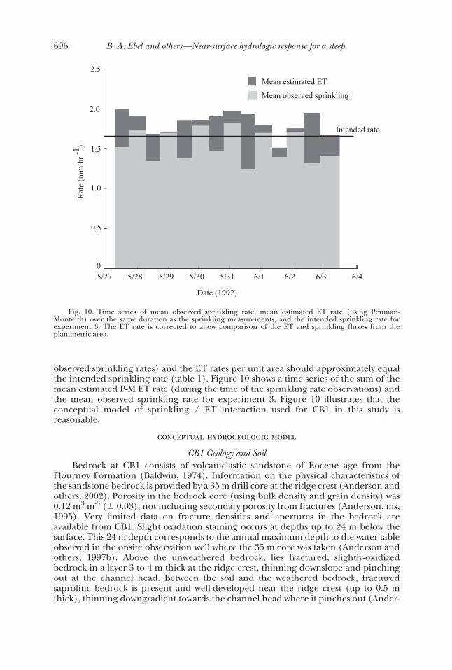
observed sprinkling rates) and the ET rates per unit area should approximately equalthe intended sprinkling rate (table 1). Figure 10 shows a time series of the sum of themean estimated P-M ET rate (during the time of the sprinkling rate observations) andthe mean observed sprinkling rate for experiment 3. Figure 10 illustrates that theconceptual model of sprinkling / ET interaction used for CB1 in this study isreasonable.

conceptual hydrogeologic model

CB1 Geology and SoilBedrock at CB1 consists of volcaniclastic sandstone of Eocene age from the

Flournoy Formation (Baldwin, 1974). Information on the physical characteristics ofthe sandstone bedrock is provided by a 35 m drill core at the ridge crest (Anderson andothers, 2002). Porosity in the bedrock core (using bulk density and grain density) was0.12 m3 m-3 (� 0.03), not including secondary porosity from fractures (Anderson, ms,1995). Very limited data on fracture densities and apertures in the bedrock areavailable from CB1. Slight oxidation staining occurs at depths up to 24 m below thesurface. This 24 m depth corresponds to the annual maximum depth to the water tableobserved in the onsite observation well where the 35 m core was taken (Anderson andothers, 1997b). Above the unweathered bedrock, lies fractured, slightly-oxidizedbedrock in a layer 3 to 4 m thick at the ridge crest, thinning downslope and pinchingout at the channel head. Between the soil and the weathered bedrock, fracturedsaprolitic bedrock is present and well-developed near the ridge crest (up to 0.5 mthick), thinning downgradient towards the channel head where it pinches out (Ander-

Fig. 10. Time series of mean observed sprinkling rate, mean estimated ET rate (using Penman-Monteith) over the same duration as the sprinkling measurements, and the intended sprinkling rate forexperiment 3. The ET rate is corrected to allow comparison of the ET and sprinkling fluxes from theplanimetric area.


son and Dietrich, 2001). While little soil profile information exists for the CB1 site, soilpits 70 m off-site reveal that the soil is a highly porous (0.5 - 0.6 m3 m-3) sandy loam(Torres, ms, 1997). The colluvial soil exhibits substantial small scale variability in soildepth (fig. 3B). The soil contains Mountain beaver (Aplodontia rufa) burrows �0.2 m indiameter reaching 1.2 to 2.0 m depth (Torres and others, 1998). Burrow networks canextend up to 100 m in length with openings every 6 to 7 m (Schmidt, ms, 1999).

Slug TestsSlug tests were performed at CB1 during the third sprinkling experiment consist-

ing of 177 falling head slug tests in piezometers emplaced in the colluvial soil,saprolite, and weathered bedrock. The piezometer design at CB1 is described byMontgomery and others (1997). Results and conclusions from the CB1 slug tests arediscussed in detail by Montgomery and others (2002). For the effort reported hereinand the companion paper (Ebel and others, 2007), the slug test data were reanalyzedusing the Bouwer and Rice (1976) method. Table 6 provides a statistical summary ofthe CB1 saturated hydraulic conductivity estimates. The values in table 6 are similar tothose reported by Montgomery and others (2002) and support their conclusions. Thestatistical differences between the saturated hydraulic conductivity estimates in table 6and the values reported by Montgomery and others (2002) are likely the result of, forthis study, separating the saprolite estimates from the weathered bedrock and soilestimates, which is consistent with the geologic characterization by Anderson andDietrich (2001). Slug test interpretation also has a subjective element relative to thechoosing of the normalized response time (see Butler, 1998) that can affect saturatedhydraulic conductivity estimates.

Montgomery and others (2002) examined the variation in saturated hydraulicconductivity estimates with depth and found: (i) an inverse relationship betweenpiezometer depth and saturated hydraulic conductivity estimates within the soil and(ii) no discernable relation between piezometer depth and saturated hydraulic conduc-tivity in the bedrock piezometers. The findings of Montgomery and others (2002) arein agreement with the saturated hydraulic conductivity estimates presented hereinplotted as a function of depth. While consistent with observations from other studiesthat observed a decline in saturated hydraulic conductivity with depth in soils, (Beven,1984; Elsenbeer and others, 1992; Ambroise and others, 1996), the correlation at CB1is too weak to develop a reliable quantitative relationship between saturated hydraulic

Table 6

Characteristics of the CB1 saturated hydraulic conductivity (Ksat) estimates for thesoil and bedrock using the Bouwer and Rice (1976) method

1The number of estimates does not include repeated measurements at the same locationthat are not included in the statistics.


conductivity and depth below the surface (Montgomery and others, 2002). It is worthnoting that the gaps in the spatial distribution of the soil slug test data, particularly inthe top 0.5 m of soil, prevent a meaningful 3D interpolation of the soil saturatedhydraulic conductivity estimates. The lack of spatial structure and the small number(see table 6) of slug tests in the saprolite and weathered bedrock does not allow for ameaningful 3D interpolation of the saturated hydraulic conductivity.

effects of sprinkling spatial variability on hydrologic response

Results from Previous Hydrologic Response Investigations at CB1During the three sprinkling experiments, piezometric, tensiometric, and dis-

charge measurements were taken repeatedly (see table 2). TDR measurements ofsoil-water content were also taken during the third experiment. Deuterium wasintroduced into the sprinkling water during the third experiment for tracer experi-ments in the vadose zone and concentrations were monitored using lysimeters(ceramic cup, tension, and plate). Discharge collected at the two weirs was analyzed fordeuterium and bromide. Previous analyses of the CB1 data have advanced theunderstanding of hydrologic-response in steep, unchanneled valleys. For example, themajor findings from Anderson and others (1997a), Montgomery and others (2002),Montgomery and Dietrich (2002) and Torres and others (1998) include: (i) theunsaturated zone delays the timing of pore-water pressure development and runoffgeneration, (ii) flow paths at the soil-saprolite-bedrock interface are important forrunoff generation at CB1 (that is, subsurface storm flow), (iii) shallow bedrockfracture flow can control pore-water pressure magnitudes at CB1, (iv) the extremelyhigh hydraulic conductivities in the soil (relative to the underlying bedrock) and steepslopes do not favor overland flow runoff generation mechanisms. The effects of spatialvariations in sprinkling intensity have not been incorporated into the previous analysesof near-surface hydrologic response at CB1, except in the estimation of deuteriumvelocities by Anderson and others (1997b). The effort reported herein examines theeffect of sprinkling spatial variability (see figs. 6, 7, 8, and 9; table 5) on the observedCB1 hydrologic response.

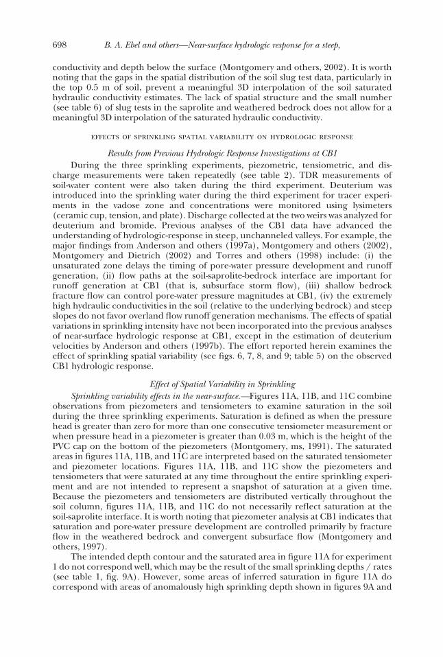
Effect of Spatial Variability in SprinklingSprinkling variability effects in the near-surface.—Figures 11A, 11B, and 11C combine

observations from piezometers and tensiometers to examine saturation in the soilduring the three sprinkling experiments. Saturation is defined as when the pressurehead is greater than zero for more than one consecutive tensiometer measurement orwhen pressure head in a piezometer is greater than 0.03 m, which is the height of thePVC cap on the bottom of the piezometers (Montgomery, ms, 1991). The saturatedareas in figures 11A, 11B, and 11C are interpreted based on the saturated tensiometerand piezometer locations. Figures 11A, 11B, and 11C show the piezometers andtensiometers that were saturated at any time throughout the entire sprinkling experi-ment and are not intended to represent a snapshot of saturation at a given time.Because the piezometers and tensiometers are distributed vertically throughout thesoil column, figures 11A, 11B, and 11C do not necessarily reflect saturation at thesoil-saprolite interface. It is worth noting that piezometer analysis at CB1 indicates thatsaturation and pore-water pressure development are controlled primarily by fractureflow in the weathered bedrock and convergent subsurface flow (Montgomery andothers, 1997).

The intended depth contour and the saturated area in figure 11A for experiment1 do not correspond well, which may be the result of the small sprinkling depths / rates(see table 1, fig. 9A). However, some areas of inferred saturation in figure 11A docorrespond with areas of anomalously high sprinkling depth shown in figures 9A and


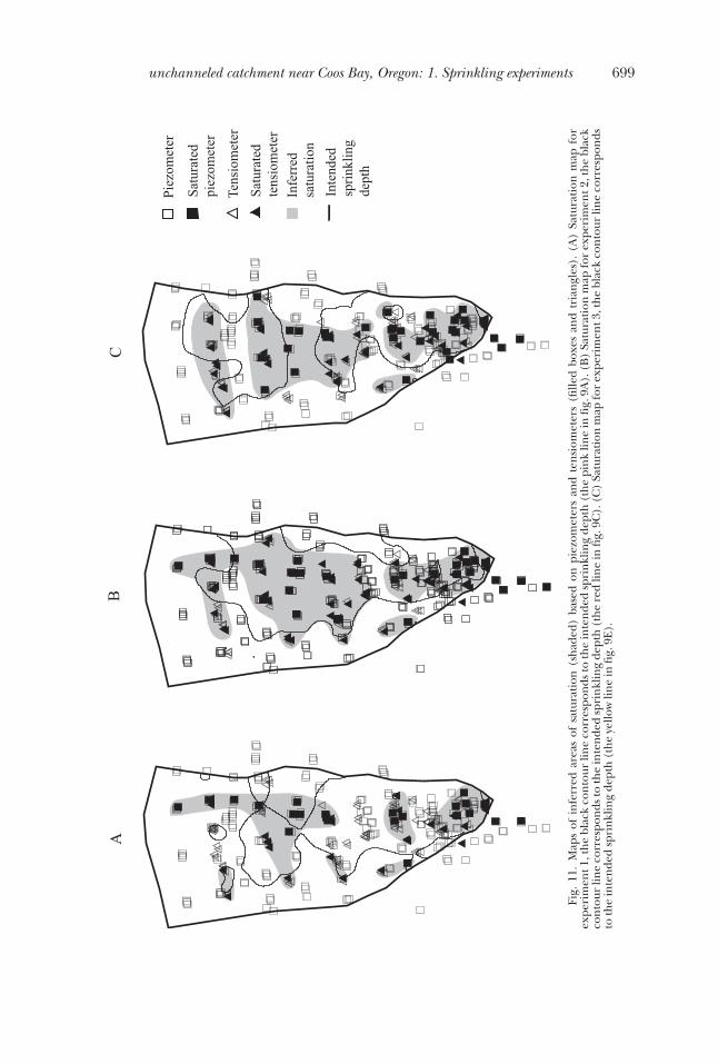
Fig.

11.

Map

sof

infe

rred

area

sof

satu

rati

on(s

had

ed)

base

don

piez

omet

ers

and

ten

siom

eter

s(fi

lled

boxe

san

dtr

ian

gles

).(A

)Sa

tura

tion

map

for

expe

rim

ent1

,th

ebl

ack

con

tour

line

corr

espo

nds

toth

ein

ten

ded

spri

nkl

ing

dept

h(t

he

pin

klin

ein

fig.

9A).

(B)

Satu

rati

onm

apfo

rex

peri

men

t2,t

he

blac

kco

nto

urlin

eco

rres

pon

dsto

the

inte

nde

dsp

rin

klin

gde

pth

(th

ere

dlin

ein

fig.

9C).

(C)

Satu

rati

onm

apfo

rex

peri

men

t3,t

he

blac

kco

nto

urlin

eco

rres

pon

dsto

the

inte

nde

dsp

rin

klin

gde

pth

(th

eye

llow

line

infi

g.9E

).


9B. For example, the saturated areas near the middle of platforms 9, 7 and 5 (see fig.3A) and near the left edge of platforms 11, 7 and 5 (see fig. 3A) correspond with highsprinkling depths shown in figures 9A and 9B. Comparison of figure 11A withpreviously reported saturation maps using piezometers (see Montgomery and others,1997) reveals that the saturated areas are similar (patchy and discontinuous), but withadditional information gained by considering tensiometer data.

Figure 11B for sprinkling experiment 2 illustrates a stronger correlation betweenthe intended sprinkling depth contour and the area of inferred saturation. Thiscorrelation is most likely the result of the higher sprinkling rates in experiment 2. Thesaturated areas in figure 11B are less patchy than in figure 11A and nearly continuousalong the surface and subsurface hollow axes (figs. 3A and 3B). Comparison ofinferred saturation to sprinkling depths (figs. 9C and 9D) shows areas of saturationdeveloping near elevated sprinkling depths near the middle of platforms 11, 9, 7, and 5(fig. 3A) and near the left side of platforms 7 and 5 (fig. 3A). Comparison of theprevious saturation maps from piezometers alone (see Montgomery and others, 1997)to figure 11B again reveals the additional information gained from consideringtensiometer data.

Figure 11C represents the interesting “compromise” of experiment 3 compared toexperiments 1 and 2 where the intended sprinkling depth in experiment 3 is almostequal to that of experiment 2 because of the longer duration while the intendedsprinkling rate is close to that of experiment 1 (table 1 and fig. 9). Visually, thecorrelation between the contour of intended sprinkling depth and the inferredsaturated area (fig. 11C) is not as strong as in experiment 2 (fig. 11B), but stillsignificant and more prominent than for experiment 1 (fig. 11A). Comparisons of theareas of concentrated sprinkling from figures 9E and 9F to the saturated areas in figure11C suggest that sprinkling heterogeneity can effect saturation development, forexample the saturated areas along platforms 11 and 9, near the middle of platforms 7and 5, and close to the left edge of platform 5 (fig. 3A).

Examination of figure 11C shows a gap in saturation between platforms 11 and 9(see fig. 3A) along the hollow axis in experiment 3, despite the connected contour ofintended depth. This suggests that the spatial continuity of sprinkling depth does nothave a large impact on the continuity of the area of subsurface saturation along thehollow axis. It is worth repeating that figures 11A, 11B, and 11C represent the entiresoil column and do not reflect saturation at the soil-saprolite interface nor do theyrepresent a snapshot of saturation at a specific point in time. Instead, figures 11A, 11B,and 11C are indicative of saturation that develops within the soil column relative tospatial and temporal variations in sprinkling intensity. In particular, the saturationnoted in the shallow tensiometers along platform 11 only lasts for several hours duringexperiment 1, 2, and 3 following locally elevated sprinkling intensities at thoselocations.

Spatial variability in tensiometric response was examined by Torres and others(1998) and no clear spatial pattern of the time to quasi-steady state, using an approachfrom Horton (1940), was found for sprinkling experiments 1 and 2. The timing toquasi-steady state for tensiometric response is defined herein, for experiment 3, as thefirst instance of consecutive decreasing pressure heads after the full arrival of thewetting front (that is, when pressure heads become near steady state). Figures 12A and12B show overlays of the tensiometer time to quasi-steady state values at the 0.25 m (�0.05 m) and 0.5 m (� 0.1 m) depths onto the Kriged sprinkling rates from the first 46hours of experiment 3. The areas of higher sprinkling rates and the areas of morerapid time to quasi-steady state in figures 12A and 12B correspond. Some of the rapidlyresponding tensiometers are located near the left edge of platform 7 (fig. 3A) wheresprinkling rates are small, which is likely the result of the shallow soils at those


tensiometers (see fig. 3B). Overall, figures 12A and 12B suggest that sprinkling ratesaffect the timing to quasi-steady state for the tensiometers in experiment 3 and explainsome of the observed spatial patterns of tensiometric response.

Sprinkling spatial variability effects at the soil-saprolite-bedrock interface.—Pore-waterpressures and saturation at the soil-saprolite interface at CB1 could depend on spatialand temporal variations in sprinkling intensity / depth. Kriged maps of pore-waterpressures from piezometers and tensiometers were created using the relation:

p � �g (6)

where p is the pore-water pressure (Pa), � is the density of water (kg m-3), g is gravity(m s-2), and � is the pressure head (m). Piezometers are capable of observingpore-water pressures above zero and tensiometers are capable of observing pore-waterpressures above and below zero (Harr, 1977; Johnson and Sitar, 1990).

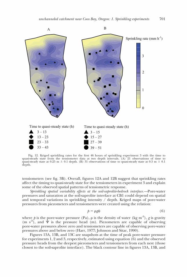
Figures 13A, 13B, and 13C are snapshots at the time of peak pore-water pressurefor experiments 1, 2 and 3, respectively, estimated using equation (6) and the observedpressure heads from the deepest piezometers and tensiometers from each nest (thoseclosest to the soil-saprolite interface). The black contour line in figures 13A, 13B, and

Fig. 12. Kriged sprinkling rates for the first 46 hours of sprinkling experiment 3 with the time toquasi-steady state from the tensiometer data at two depth intervals. (A) 21 observations of time toquasi-steady state at 0.25 m � 0.1 depth. (B) 31 observations of time to quasi-steady state at 0.5 m � 0.1depth.


13C marks the line of saturation (pore-water pressure equal to zero) at the soil-saprolite interface at the time of peak pore-water pressure. Comparison of figures 11A,11B, and 11C to figures 13A, 13B, and 13C reveals the difference between saturation atany location throughout the soil column at any time during the experiment comparedto saturation at the soil-saprolite interface at a specific point in time (snapshot).Figures 13A and 13C show that saturation is primarily developed near the hollow axisof the soil-saprolite interface (see fig. 3B). The saturation development (figs. 13A and13C) is likely the result of convergent subsurface flow (Anderson and Burt, 1978;Montgomery and others, 1997; Freer and others, 2002), during experiments 1 and 3.Figure 13B shows that saturation at the soil-saprolite interface during the secondsprinkling experiment develops near the subsurface hollow axis (fig. 3B) but extendsover a larger area than figures 13A and 13C. In Figure 13B there are undoubtedlyKriging artifacts in areas where there is less data that show saturation reaching theridge crest and at the left boundary that are not real. The saturated areas in figures 13Aand 13C compare well with the saturated areas shown by Montgomery and others(1997, 2002), with additional understanding gained by considering tensiometer data.

Figures 13A, 13B, and 13C also suggest that pore-water pressure magnitudes maybe affected by sprinkling intensity, which is consistent with field and laboratoryobservations (for example, Johnson and Sitar, 1990; Marui and others, 1993; Reid andothers, 1997). For example the pore-water pressure hotspots in figures 13A, 13B, and13C along the middle of platforms 9, 7 and 5 (see fig. 3A) correspond with areas ofconcentrated sprinkling in figures 9A, 9C, and 9E.

Effect of Sprinkling Spatial Variability on Water Balance CalculationsSeveral water-balance calculations have been conducted for the CB1 sprinkling

experiments (see Anderson, ms, 1995; Montgomery and others, 1997; Torres, ms,1997) using a variety of techniques to approximate the fluxes into and out of thecatchment. Only the water balance of Torres (ms, 1997) considered spatially variable

Fig. 13. Kriged snapshots of pore-water pressures based upon data from the piezometers and tensiom-eters closest to the soil-saprolite interface. (A) Peak pore-water pressures from experiment 1 at 10:00 PM on5/13/1990. (B) Peak pore-water pressures from experiment 2 at 9:00 AM on 5/27/1990. (C) Peakpore-water pressures from experiment 3 at 10:00 AM on 5/31/1992.


input (sprinkling) and storage by dividing up the catchment into 5 areas for calculat-ing spatially variable sprinkling and unsaturated soil-water storage (using TDR watercontents) and incorporated the piezometer data to calculate saturated soil storage. Acritical difference between the previously reported water balances and the onereported herein for experiment 3 is the use of all the observed manual rain gage data(and the corresponding exclusion of ET). If the observed sprinkling rate is equivalentto the intended sprinkling rate less the ET (as suggested by fig. 10), then the amount ofwater entering the catchment subsurface is approximately the same in the waterbalance reported here as in the previous studies (albeit not uniformly distributed inspace).

The water balance results for this study represent the spatial variability in soil-water storage by combining nearby piezometer and tensiometer nests to producepressure head profiles of the soil. Thirty piezometer / tensiometer groups wereselected and the catchment was divided, with Thiessen (Voronoi) polygons, aroundthose groups. The soil depth from the deepest piezometer in each group was then usedto approximate the soil depth across the entire polygon. Interpolation between theobserved pressure heads from the tensiometers and piezometers provided an estimateof the pressure head with depth profile for each polygon. The estimated pressure headprofiles were converted to soil-water contents using the van Genuchten (1980) methodand numerically integrated with respect to soil depth to give water content (m) foreach polygon. When multiplied by the area of the polygon, the volume of water storedresults. This calculation was made at the start of sprinkling experiment 3 (5/27/1992,10:00 AM) and after the sprinkling experiment had ended when discharge from boththe upper and lower weirs was almost zero (6/7/1992, 11:15AM). The calculatedstorages were 186 m3 and 201 m3 at the start and end of the experiment, respectively. Acheck of the water contents from the interpolation of the piezometer and tensiometerdata using measured soil-water contents from nearby TDR data (where available) wereonly different (the mean of the absolute values of all the estimated minus observedsoil-water contents) by 0.04 [m3 m-3] at the start of the third experiment. Unfortu-nately, no TDR data are available on 6/7/1992 to check the estimated soil-watercontents at the end of the experiment. The difference between the starting and endingsoil-water storage estimates indicates that approximately 15 m3 of water was left instorage in the soil four days after sprinkling ended.

Using the estimate of stored soil water, it is possible to calculate the water balancefor experiment 3 as:

I � R � �L � �Sb� � �Ss � 0 (7)

where I is the irrigation [m3] (sprinkling), R is the runoff [m3], L is the leakage [m3] toa regional groundwater system, �Sb is the change in saprolite and bedrock storage[m3], �Ss is the change in soil storage [m3]. The principal assumption employed inequation (7) is that deep leakage is closely linked with the amount of water going tobedrock storage. Equation (7) can be rearranged to solve for the combined term ofdeep leakage / bedrock storage as the residual in the water balance. The cumulativevolume of water from the experiment 3 Kriged sprinkling total in figure 9E is 215 m3,the cumulative runoff is 129 m3, and the soil-water storage at the end of the waterbalance period is 15 m3, yielding a residual of 71 m3. Dividing the 71 m3 residual by theduration of the water balance period, 265.25 hours, and then dividing by the planimet-ric area of the catchment gives an estimate of the rate at which water goes into bedrockstorage / leaks of 8.7 x 10-8 m s-1 or 0.31 mm h-1. The bedrock storage / leaking ratecalculated herein using equation (7) of 0.31 mm h-1 is approximately equal to the deepleakage rate calculated by Anderson and Dietrich (2001) of 0.32 mm h-1. Assuming aunity hydraulic gradient, the leakage rate provides a first-order estimate of the


saturated hydraulic conductivity of the deep bedrock. Although the methodologyemployed herein is slightly different than that employed in previous CB1 waterbalances, the incorporation of spatial variability in sprinkling and soil-water contentdoes not significantly change the water balance calculation.

discussionData limitations exist in some the hydrologic-response analyses reported here. For

example, capturing the spatial variations in sprinkling necessitates using the manualrain gage data, despite the limited temporal resolution. Previous research at CB1suggests that small-scale temporal variations in sprinkling can significantly affecthydrologic response (Torres and others, 1998). However, the results presented hereillustrate that spatial variability in sprinkling affects hydrologic response and that thesprinkling rates from the higher temporal resolution automated gages (see fig. 5) areinaccurate due to undercatch. The evaluation of natural rainfall variability relative tosprinkling variability was only analyzed for two natural storms and three sprinklingexperiments; more research on this subject would further identify the differencesbetween sprinkling and rainfall and how to account for / approximate these differ-ences in analysis and simulation of hydrologic response. An additional limitation is thespatial distribution of saturated hydraulic conductivity estimates in the subsurface thatprevents meaningful spatial interpolation. For example, bedrock saturated hydraulicconductivity variations at CB1 can control pore-water pressure generation (Montgom-ery and others, 1997), but spatial variations in saturated hydraulic conductivity werenot included in the analyses presented here.

There are also limitations to the methods employed herein. One potentialweakness is the reliance on Kriging to provide realistic interpolated values of differenthydrologic observations (for example, rainfall depths / intensities, soil depths, andpore-water pressures). The drawbacks of Kriging include that it (i) has a tendency tosmooth variations in the data (loses roughness), (ii) does not perform well in areaswhere there is little data (see the areas of saturation in fig. 13B near the ridgeline), (iii)relies on the semivariogram to provide an accurate portrayal of data structure, and (iv)produces only one realization of the interpolated attribute. However, visualization ofspatially variable attributes requires some method of interpolation and, when providedwith enough data (such as 148 rain gages), Kriging provides a reliable quantitativecharacterization. When less data is available (30 or so points across the entire CB1catchment), we have qualified our results by explicitly stating that the interpolation isbest viewed in a qualitative sense. For example, it would be unwise to use Krigedpore-water pressure snapshots, like those shown in figures 13A, 13B, and 13C, to drive a3D slope stability assessment. Another potential weakness of the method employed inthis paper is the limited physical representation of the P-M ET method relative to themeteorological complexity of the sprinkling experiments. For example, the input ofsprinkling water with a different (but unknown) temperature than the air is asignificant complication to the energy balance used to formulate the P-M method.However, the data does not exist to apply more complicated ET models at CB1 and theP-M method represents most of the energy balance correctly.

Previous field and modeling studies have suggested that convergent surface andsubsurface topography is the dominant controlling factor of saturation and pore-waterpressure generation (for example, Anderson and Burt, 1978; Sidle and others, 1985;Mirus and others, 2007). Examination of figures 3A and 3B and figures 9A, 9B, 9C, 9D,9E, and 9F illustrates that areas of high sprinkling depths / intensities are concentratedalong the surface and subsurface hollow axes. The collocation of the hollow axes andelevated sprinkling depths prevents definitively separating the magnitude of thehydrologic effects of convergent subsurface flow and sprinkling heterogeneity at CB1.However, it is still clear that sprinkling heterogeneity affects hydrologic response,


although likely to a lesser extent than convergent subsurface flow. It is worth notingthat if the saturation is perched at the soil-saprolite interface (or another impedinglayer below), then that saturation development depends critically on the sprinklingrate because if the sprinkling is less than the saturated hydraulic conductivity of theperching layer, then no saturation will develop.

The major conclusions from previous work at CB1 remain unchanged by theeffort reported here. Instead, some of the nuances of hydrologic-response wereexamined with respect to sprinkling spatial variability. Quantitative spatial analyses ofthe observed CB1 hydrologic response provide the foundation for the physics-basedhydrologic-response simulations reported in the companion paper (Ebel and others,2007).

summary

The analyses presented herein indicate that simulated rainfall is more spatiallyvariable than natural storms at CB1 and that detailed spatial characterization ofsprinkling intensity is worthwhile. Experimental semivariograms of sprinkling ratesoffer a more comprehensive measure of spatial variability and continuity than eitherunivariate statistics (such as the CU, CV, and SD) or more qualitative methods ofspatial variability (such as contour maps of interpolated rates). Reproducing the spatialcharacteristics (that is, continuity, structure, and variance) of natural rainfall at a givenstudy site is a useful benchmark for evaluating rainfall simulators. Careful measure-ment of the sprinkling depths at CB1, combined with ET estimation, allows theeffective rainfall (with ET losses already removed) to be approximated by the amountobserved in the manual rain gages. The CB1 water balance calculations were notsignificantly changed by incorporating spatial variability in sprinkling rates or soil-water storage. Both tensiometric response and saturation within the CB1 near-surfacesoil profile are affected by sprinkling heterogeneity. Pore-water pressure and satura-tion development deep in the CB1 soil (at the soil-saprolite-bedrock interface) aremore sensitive to convergent flow driven by subsurface topography, but are stillsensitive to sprinkling spatial heterogeneity. Previous analyses (Montgomery andothers, 1997) demonstrate that pore-water pressure generation is also affected bybedrock saturated hydraulic conductivity variations controlled by fracture locations.Spatial variability in sprinkling rates should be incorporated into hydrologic-responsemodels designed to predict subsurface saturation and pore-water pressure develop-ment when employed in physics-based simulation of hydrologic response of sprinklingexperiments, such as the effort reported in the companion paper (Ebel and others,2007).

acknowledgmentsThe work reported herein was supported by National Science Foundation Grant

EAR-0409133. The presentation in this paper has benefited from the thoughtfulcomments of Steve Loheide, Steve Burges, Ben Mirus, Chris Heppner, and AdrianneCarr. Jef Caers provided valuable insight into geostatistical analysis. Kevin Schmidtsupplied additional data on the soil and saprolite depths. Obviously, the researchreported herein and in the companion paper would not have been possible withoutthe data collection at CB1 more than a decade ago, which was greatly facilitated byJohn Heffner. The clarity of the paper was improved by the comments of Keith Bevenand two anonymous reviewers.

AppendixThe latent heat of vaporization (MJ kg-1) was approximated as a function of the water temperature (Ts),

in C°, as (Harrison, 1963):


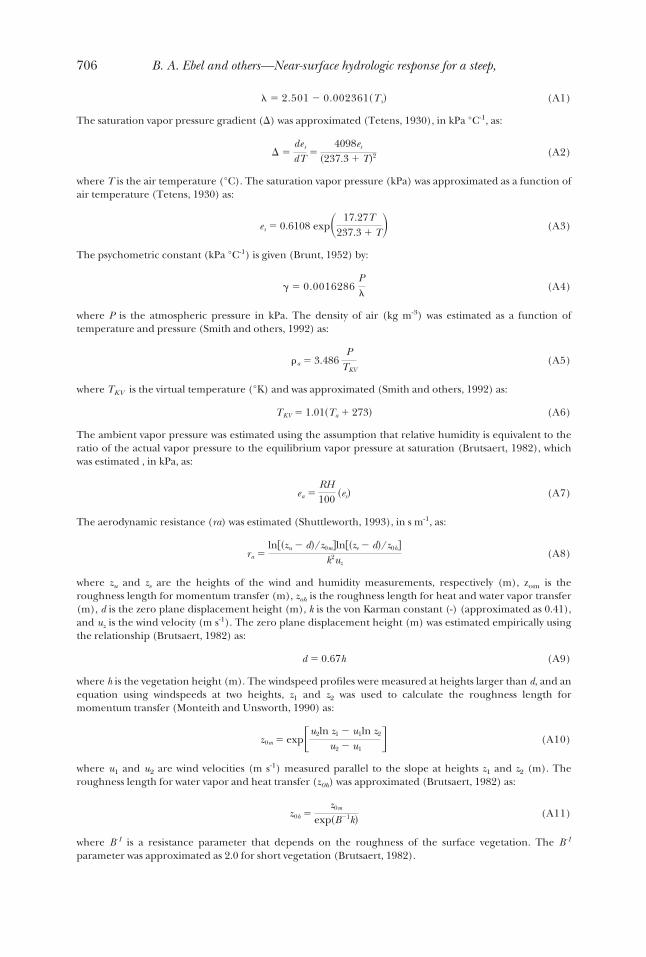
� � 2.501 � 0.002361�Ts� (A1)

The saturation vapor pressure gradient (�) was approximated (Tetens, 1930), in kPa °C-1, as:

� �des

dT�

4098es

�237.3 � T�2 (A2)

where T is the air temperature (°C). The saturation vapor pressure (kPa) was approximated as a function ofair temperature (Tetens, 1930) as:

es � 0.6108 exp� 17.27T237.3 � T� (A3)

The psychometric constant (kPa °C-1) is given (Brunt, 1952) by:

� 0.0016286P�

(A4)

where P is the atmospheric pressure in kPa. The density of air (kg m-3) was estimated as a function oftemperature and pressure (Smith and others, 1992) as:

�a � 3.486P

TKV(A5)

where TKV is the virtual temperature (°K) and was approximated (Smith and others, 1992) as:

TKV � 1.01�Ta � 273� (A6)

The ambient vapor pressure was estimated using the assumption that relative humidity is equivalent to theratio of the actual vapor pressure to the equilibrium vapor pressure at saturation (Brutsaert, 1982), whichwas estimated , in kPa, as:

ea �RH100

�es� (A7)

The aerodynamic resistance (ra) was estimated (Shuttleworth, 1993), in s m-1, as:

ra �ln�zu � d�/z0m�ln�ze � d�/z0h�

k2uz(A8)

where zu and ze are the heights of the wind and humidity measurements, respectively (m), zom is theroughness length for momentum transfer (m), zoh is the roughness length for heat and water vapor transfer(m), d is the zero plane displacement height (m), k is the von Karman constant (-) (approximated as 0.41),and uz is the wind velocity (m s-1). The zero plane displacement height (m) was estimated empirically usingthe relationship (Brutsaert, 1982) as:

d � 0.67h (A9)

where h is the vegetation height (m). The windspeed profiles were measured at heights larger than d, and anequation using windspeeds at two heights, z1 and z2 was used to calculate the roughness length formomentum transfer (Monteith and Unsworth, 1990) as:

z0m � exp�u2ln z1 � u1ln z2

u2 � u1� (A10)

where u1 and u2 are wind velocities (m s-1) measured parallel to the slope at heights z1 and z2 (m). Theroughness length for water vapor and heat transfer (z0h) was approximated (Brutsaert, 1982) as:

z0h �z0m

exp�B�1k�(A11)

where B-1 is a resistance parameter that depends on the roughness of the surface vegetation. The B-1

parameter was approximated as 2.0 for short vegetation (Brutsaert, 1982).


references

Ambroise, B., Beven, K., and Freer, J., 1996, Toward a generalization of the TOPMODEL concepts:topographic indices of hydrologic similarity: Water Resources Research, v. 32, p. 2135–2145.

Anderson, M. G., and Burt, T. P., 1978, The role of topography in controlling throughflow generation: EarthSurface Processes and Landforms, v. 3, p. 331–344.

Anderson, S. P., ms, 1995, Flow paths, solute sources, weathering, and denudation rates: The chemicalgeomorphology of a small catchment: Berkeley, California, University of California, Berkeley, Ph. D.thesis, University of California, 380 p.

Anderson, S. P., and Dietrich, W. E., 2001, Chemical weathering and runoff chemistry in a steep headwatercatchment: Hydrological Processes, v. 15, p. 1791–1815.

Anderson, S. P., Dietrich, W. E., Torres, R., Montgomery, D. R., and Loague, K., 1997a, Concentrationdischarge relationships in runoff from a steep, unchanneled catchment: Water Resources Research,v. 33, p. 211–225.

Anderson, S. P., Dietrich, W. E., Montgomery, D. R., Torres, R., Conrad, M. E., and Loague, K., 1997b,Subsurface flowpaths in a steep, unchanneled catchment: Water Resources Research, v. 33, p. 2637–2653.

Anderson, S. P., Dietrich, W. E., and Brimhall, G. H., 2002, Weathering profiles, mass-balance analysis, andrates of solute loss: Linkages between weathering and erosion in a small, steep catchment: GSA Bulletin,v. 114, p. 1143–1158.

Ascough, G. W., and Kiker, G. A., 2002, The effect of irrigation uniformity on irrigation water requirements:Water South Africa, v. 28, p. 235–242.

Baldwin, E. M., 1974, Eocene stratigraphy of southwestern Oregon: Bulletin of the Oregon Department ofGeology and Mineral Industries, v. 83, p. 1–38.

Beven, K. J., 1984, Infiltration into a class of vertically nonuniform soils: Hydrologic Sciences Journal, v. 29,p. 425–434.

Bouwer, H., and Rice, R. C., 1976, A slug test for determining hydraulic conductivity of unconfined aquiferswith completely or partially penetrating wells: Water Resources Research, v. 12, p. 423–428.

Brunt, D., 1952, Physical and dynamical meteorology, 2nd edition: Cambridge, University Press, p. 428.Brutsaert, W., 1982, Evaporation into the atmosphere: Theory, history, and applications: Dordrecht,

Holland, Reidel Publishing, 299 p.Butler, J. J., Jr., 1998, The design, performance, and analysis of slug tests: New York, Lewis Publishers, 252 p.Christiansen, J. E., 1942, Irrigation by sprinkling: California Agricultural Experiment Station Bulletin, n.

670.Croke, J., Hairsine, P., and Fogarty, P., 1999, Runoff generation and re-distribution in logged eucalyptus

forests, south-eastern Australia: Journal of Hydrology, v. 216, p. 56–77.Ebel, B. A., and Loague, K., 2006. Physics-based hydrologic-response simulation: Seeing through the fog of

equifinality: Hydrological Processes, v. 20, p. 2887–2900.Ebel, B. A., Loague, K., VanderKwaak, J. E., Dietrich, W. E., Montgomery, D. R., Torres, R., and Anderson,

S. P., 2007, Near-surface hydrologic response for a steep, unchanneled catchment near Coos Bay,Oregon: 2. Comprehensive physics-based simulations: American Journal of Science, v. 307, p. 709–748.

Elsenbeer, H., Cassel, K., and Castro, J., 1992, Spatial analysis of soil hydraulic conductivity in a tropical forestcatchment: Water Resources Research, v. 28, p. 3201–2143.

Esteves, M. E, Planchon, O., Lapetite, J. M., Silvera, N., and Cadet, P., 2000, The ‘EMIRE’ large rainfallsimulator: design and field testing: Earth Surface Processes and Landforms, v. 25, p. 681–690.

Freer, J., McDonnell, J. J., Beven, K. J., Peters, N. E., Burns, D. A., Hooper, R. P., Aulenbach, B., and Kendall,C., 2002, The role of bedrock topography on subsurface storm flow: Water Resources Research, v. 12,p. 1269–1284.

Gilbert, G. K., 1877, Report on the geology of the Henry Mountains: Washington, D. C., GovernmentPrinting Office, 170 p.

Hall, M. J., 1970, A critique of methods of simulating rainfall: Water Resources Research, v. 6, p. 104–1114.Harr, R. D., 1977, Water flux in soil and subsoil on a steep forested slope: Journal of Hydrology, v. 33,

p. 37–58.Harrison, L. P., 1963, Fundamental concepts and definitions relating to humidity, in Wexler, A., editor,

Humidity and Moisture, v. 3: New York, Reinhold Publishing Company, p. 3–70.Hornberger, G. M., Germann, P. F., and Beven, K. J., 1991, Throughflow and solute transport in an isolated

sloping soil block in a forested catchment: Journal of Hydrology, v. 124, p. 81– 99.Horton, R. E., 1940, An approach towards the physical interpretation of infiltration-capacity: Soil Science

Society of America Proceedings, v. 5, p. 399–417.Johnson, K. A., and Sitar, N., 1990, Hydrologic conditions leading to debris-flow initiation: Canadian

Geotechnical Journal, v. 27, p. 789–801.Kincaid, D. C., 1996, Spraydrop kinetic energy from irrigation sprinklers: Transactions of the ASAE, v. 17,

p. 839–845.Lane, P. N. J., Croke, J., and Dignan, P., 2004, Runoff generation and burnt convergent hillslopes: rainfall

simulation and modeling: Hydrological Processes, v. 18, p. 879–892.Lascelles, B., Favis-Mortlock, D. T., Parsons, A. J., and Guerra, A. J. T., 2000, Spatial and temporal variation in

two rainfall simulators: implications for spatially explicit rainfall simulation experiments: Earth SurfaceProcesses and Landforms, v. 25, p. 709–721.

Loch, R. J., Robotham, B. G., Zeller, L., Masterman, N., Orange, D. N., Bridge, B. J., Sheridan, G., andBourke, J. J., 2001, A multi-purpose rainfall simulator for field infiltration and erosion studies:Australian Journal of Soil Research, v. 39, p. 599–610.


Luk, S. H., Abrahams, A. D., and Parsons, A. J., 1983, Sediment sources and sediment transport by rill flowand interrill flow on a semi-arid piedmont slope, Southern Arizona: Catena, v. 20, p. 93 –111.

Marui, A., Yasuhara, M., Kuroda, K., and Takayama, S., 1993, Subsurface water movement and transmissionof rainwater pressure through a clay layer, in Gladwell, J. S., editor, Hydrology of Warm Humid Regions:Wallingford, United Kingdom, IAHS Press, v. 216, p. 463–470.

Mirus, B. B., Ebel, B. A., Loague, K., and Wemple, B. C., 2007, Simulated effect of a forest road onnear-surface hydrologic response: redux: Earth Surface Processes and Landforms, v. 32, p. 126–142,

Monteith, J. L., 1965, Evaporation and environment: The State and Movement of Water in Living Organisms,Symposium of the Society for Experimental Biology, n. 19, p. 205-234.

Monteith, J. L., and Unsworth, M. H., 1990, Principles of environmental physics: New York, Edward Arnold,291 p.

Montgomery, D. R., ms, 1991, Channel initiation and landscape evolution : Berkeley, California, Universityof California, Berkeley, Ph. D. thesis, 421 p.

Montgomery, D. R., and Dietrich, W. E., 2002, Runoff generation in a steep, soil-mantled landscape: WaterResources Research, v. 38, p. 1168–1175.

Montgomery, D. R., Dietrich, W. E., Torres, R., Anderson, S. P., Heffner, J. T., and Loague, K., 1997,Hydrologic response of a steep, unchanneled valley to natural and applied rainfall: Water ResourcesResearch, v. 33, p. 91–109.

Montgomery, D. R., Dietrich, W. E., and Heffner, J. T., 2002, Piezometric response in shallow bedrock at CB1:Implication for runoff generation and landsliding: Water Resources Research, v. 38, p. 1274–1292.

Motha, J. A., Wallbrink, P. J., Hairsine, P. B., and Grayson, R. B., 2002, Tracer properties of eroded sedimentand source material: Hydrologic Processes, v. 16, p. 1983–2000.

Newson, A. J., and Clarke, R. T., 1976, Comparison of the catch of ground-level and canopy-level rain-gaugesin the Upper Severn Experimental Catchment: Meteorological Magazine, v. 105, p. 2–7.

Parsons, A. J., Stromberg, S. G. L., and Greener, M., 1998, Sediment-transport competence of rain-impactedinterill overland flow: Earth Surface Processes and Landforms, v. 23, p. 365– 375.

Reid, M. E., LaHusen, R. G., and Iverson, R. M., 1997, Debris flow initiation experiments using diversehydrologic triggers, in Chen, C. L., editor, Debris Flow Hazards Mitigation: Mechanics, Prediction andAssessment, ASCE Proceedings, p. 1–11.

Riley, S. J., and Hancock, F., 1997, A rainfall simulator for hydrologic and erosion experiments on mines,with an example of its applications at Ranger Uranium Mine, Northern Territory, Australia: TheAustralasian Institute of Mining and Metallurgy Proceedings, v. 1, p. 3–8.

Rodda, J. C., and Smith, S. W., 1986, The significance of systematic error in rainfall measurement forassessing wet deposition: Atmospheric Environment, v. 20, p. 1059–1064.

Schmidt, K. M., ms, 1999, Root strength, colluvial soil depth, and colluvial transport on landslide-pronehillslopes: Seattle, Washington, University of Washington, Seattle, Ph. D. thesis, 258 p.

Seginer, I., Kantz, D., and Nir, D., 1991, The distortion by wind of the distribution patterns of singlesprinklers: Agricultural Water Management, v. 19, p. 341–359.

Sharpley, A., and Kleinman, P., 2003, Effect of rainfall simulator and plot scale on overland flow andPhosphorus transport: Journal of Environmental Quality, v. 32, p. 2172–2179.

Shuttleworth, W. J., 1991, Evaporation models in hydrology, in Schmugge, T. J., and Andre, J., editors, Landsurface evaporation : measurement and parameterization: New York, Springer Verlag, p. 93–120.

–––––– 1993, Evaporation, in Maidment, D., editor, Handbook of Hydrology: New York, McGraw HillPublishers, p. 4.1–4.53.

Sidle, R. C., Pearce, A. J., and O’Loughlin, C. L., 1985, Hillslope stability and land use: Washington D. C.,American Geophysical Union, Water Resources Mongraph, v. 11, 140 p.

Smith, M., Allen, R. G., Monteith, J. L., Perrier, A., Pereira, L., and Segeren, A., 1992, Report of the expertconsultation on procedures for revision of FAO guidelines for prediction of crop water requirements:UN-FAO, Rome, Italy, 54 p.

Sumner, H. R., Wauchope, R. D., Truman, C. C., Dowler, C. C., and Hook, J. E., 1996, Rainfall simulator andplot design for mesoplot runoff studies: Transactions of the American Society of Agricultural Engineers,v. 39, p. 125–130.

Tarjuelo, J. M., Ortega, J. F., Montero, J., and de Juan, J. A., 2000, Modelling evaporation and drift losses inirrigation with medium size impact sprinklers under semi-arid conditions: Agricultural Water Manage-ment, v. 43, p. 263–284.

Taylor, G., Hale, C., and Joos, S., 2005, Climate of Coos County, Special report, Oregon Climate Service:Corvallis, Oregon, Oregon State University, p. 1–4.

Tetens, O., 1930, Uber einige meteorologische Begriffe: Zeitschrift fur Geophysik, v. 6, p. 297–309.Torres, R., ms, 1997, Unsaturated zone processes and the hydrologic response of a steep, unchanneled

valley: Berkeley, California, University of California, Berkeley, Ph. D. thesis, 298 p.Torres, R., Dietrich, W. E., Montgomery, D. R., Anderson, S. P., and Loague, K., 1998, Unsaturated zone

processes and the hydrologic response of a steep, unchanneled catchment: Water Resources Research,v. 34, p. 1865–1879.

van Genuchten, M. Th., 1980, A closed-form equation for predicting the hydraulic conductivity ofunsaturated soils: Soil Science Society of America, v. 44, p. 892–898.

Waddington, J. M., and Devito, K. J., 2001, Portable irrigation system for studying hillslope and wetlandrunoff generation processes: Hydrological Processes, v. 15, p. 281–287.

Wilson, C. J., 1999, Effects of logging and fire on runoff and erosion on highly erodible granitic soils inTasmania: Water Resources Research, v. 35, p. 3531–3556.

Wisler, C. O., and Brater, E. F., 1959, Hydrology: New York, John Wiley, 408 p.Yazar, A., 1984, Evaporation and drift losses from sprinkler irrigation systems under various operating

conditions: Agricultural Water Management, v. 8, p. 439–449.

708 B. A. Ebel and others708

near-surface hydrologic response for a steep, unchanneled

Documents