NEC Program Description - Theory

Version 1.0

August 18, 2007

compiled by

Chuck Adams, K7QO

k7qo@commspeed.net

Numerical Electromagnetics Code (NEC) Method

of Moments

Part I: Program Description - Theory

A user-oriented computer code for analysis of theelectromagnetic response of antennas and other metal structures

Part I: Program Description - TheoryPart II: Program Description - Code

(Volume 2 contains Part III: User’s Guide)

GJ Burke and AJ Pogio(Lawrence Livermore Laboratory)

January 1981

Prepared by LAWRENCE LIVERMORE LABORATORY (Report UCID 18834)Prepared by NAVAL ELECTRONIC SYSTEMS COMMAND (NAVELEX 3041)Approved for public release; distribution unlimited

NAVAL OCEAN SYSTEMS CENTERSAN DIEGO, CALIFORNIA 92151

This manual and the associated NEC-2 manuals are the result of a

concerted effort to produce a set of clean documents for the NEC-2

program. The original manuals were first released in January 1981 and

are available from the US Government, but are of poor quality. Not the

fault of any individual or group. It is just an illustration of the

evolution of computer technology since the time of using typewriters

for the production of manuals and documentation. The original manuals

are also available online from several sources by doing a search for

nec2part1.pdf, nec2part2.pdf, and nec2part3.pdf.

I have made an effort to correct as many errors as possible in the

scanning of the documents and the OCR process itself. Any pointers to

errors, either in the original documents or in my production of these

documents is greatly appreciated. I will make the appropriate corrections

and reproduce the new document as soon as possible and place them back on

the web.

These documents were produced using LaTeX under the kubuntu 7.04 Linux

operating system on a Compaq Presario AMD 64 system. I have redone all

the graphics where possible to improve the quality of the documents. This

work started in mid-June 2007 and most likely will continue for a very

long time due to the immensity of the project.

I have chosen the fixed spacing typewriter font to reproduce the font

used in the original documents.

The program listing is slightly different from the original as shown in

Part II of the original manual, so it will take a long time to match the

program line numbers with the correct lines. Just please patient as this

work progresses.

Please note that all equations have been entered entirely by hand and

are subject to extra scrutiny on the part of the reader.

Thanks.

Chuck Adams

Prescott, AZ

June, 2007

k7qo@commspeed.net

ii

Preface

The Numerical Electromagnetics Code (NEC) has been developed at the Lawrence Livermore

Laboratory, Livermore, California, under the sponsorship of the Naval Ocean Systems

Center and the Air Force Weapons Laboratory. It is an advanced version of the Antenna

Modeling Program (AMP) developed in the early 1970’s by MBAssociates for the Naval

Research Laboratory, Naval Ship Engineering Center, U.S. Army ECOM/Communications Systems,

U.S. Army Strategic Communications Command, and Rome Air Development Center under Office

of Naval Research Contract N00014-71-C-0187. The present version of NEC is the result

of efforts by G. J. Burke and A. J. Poggio of Lawrence Livermore Laboratory.

The documentation for NEC consists of three volumes:

• Part I: NEC Program Description - Theory

• Part II: NEC Program Description - Code

• Part III: NEC User’s Guide

The documentation has been prepared by using the AMP documents as foundations and

by modifying those as needed. In some cases this led to minor changes in the original

documents while in many cases major modifications were required.

Over the years many individuals have been contributors to AMP and NEC and are acknowledged

here as follows:

R. W. Adams E. K. Miller

J. N. Brittingham J. B. Morton

G. J. Burke G. M. Pjerrou

F. J. Deadrick A. J. Poggio

K. K. Hazard E. S. Selden

D. L. Knepp

D. L. Lager

R. J. Lytle

The support for the development of NEC-2 at the Lawrence Livermore Laboratory has

been provided by the Naval Ocean Systems Center under MIPR-N0095376MP. Cognizant individuals

under whom this project was carried out include: J. Rockway and J. Logan.

Previous development of NEC also included the support of the Air Force Weapons

Laboratory (Project Order 76-090) and was monitored by J. Castillo and TSgt. H. Goodwin.

Work was performed under the auspices of the U. S. Department of Energy under contract

No. W-7405-Eng-48. Reference to a company or product name does not imply approval

or recommendation of the product by the University of California or the U. S. Department

of Energy to the exclusion of others that may be suitable.

iii

CONTENTS

Section Page

I. INTRODUCTION ................................................................... 1

II. THE INTEGRAL EQUATIONS FOR FREE SPACE .......................................3

l. The Electric Field Integral Equation (EFIE) ............................ 3

2. The Magnetic Field Integral Equation (MFIE)............................. 5

3. The EFIE-MFIE Hybrid Equation ............................................ 7

III. NUMERICAL SOLUTION ...........................................................8

l. Current Expansion on Wires ............................................... 9

2. Current Expansion on Surfaces ........................................... 17

3. Evaluation of the Fields ................................................ 20

4. The Matrix Equation for Current ........................................ 29

5. Solution of the Matrix Equation ........................................ 30

IV. EFFECT OF A GROUND PLANE .................................................... 35

l. The Sommerfield/Norton Method ........................................... 36

2. Numerical Evaluation of the Sommerfield Integrals .................... 51

3. The Image and Reflection-Coefficient Methods ......................... 55

V. MODELING OF ANTENNAS ..........................................................61

1. Source Modeling .......................................................... 61

2. Nonradiating Networks .................................................... 67

3. Transmission Line Modeling .............................................. 72

4. Lumped or Distributed Loading ........................................... 74

5. Radiated Field Calculation .............................................. 76

6. Antenna Coupling ......................................................... 78

REFERENCES .........................................................................79

iv

LIST OF ILLUSTRATIONS

Figure Page

1. Current Basis Functions and Sums on a Four Segment Wire ................... 10

2. Segments Covered by the i-th Basis Function ................................. 10

3. Detail of the Connection of a Wire to a Surface ............................ 16

4. Current-Filament Geometry for the Thin-Wire Kernel ......................... 17

5. Current Geometry for the Extended Thin-Wire Kernel ......................... 19

6. Coordinates for Evaluating the Field of a Current Element Over Ground ... 31

7. IVρ for ǫ1/ǫ0 = 4, σ1 = 0.001 mhos/m, frequency = 10MHz ....................... 37

8. IVz for ǫ1/ǫ0 = 4, σ1 = 0.001 mhos/m, frequency = 10MHz ....................... 38

9. IHρ for ǫ1/ǫ0 = 4, σ1 = 0.001 mhos/m, frequency = 10MHz ....................... 39

10. IHφ for ǫ1/ǫ0 = 4, σ1 = 0.001 mhos/m, frequency = 10MHz ....................... 40

11. IHρ for ǫ1/ǫ0 = 16, σ1 = 0.0 mhos/m, frequency = 10MHz ........................ 41

12. Grid for Bivariate Interpolation of I’s ..................................... 43

13. Contour for Evaluation of Bessel Function Form of Sommerfeld Integrals .. 51

14. Contour for Evaluation of Hankel Function Form of Sommerfeld Integrals .. 53

15. Contour for Evaluation of Hankel Function Form when Real Part k1

is Large and Imaginary Part k1 is Small ...................................... 54

16. Plane-Wave Reflection at an Interface ........................................ 49

17. Biconical Transmission Line Model of Source Region ......................... 55

18. Field Plots for a Linear Dipole, Ω=15 ....................................... 58

19. Voltage and Current Reference Direction at Network Ports .................. 60

20. Network Connection to Segments ................................................ 60

21. Network Port and Voltage Source Connected to a Segment .................... 61

22. Current Distribution on a Two-Wire Transmission Line ....................... 64

v

Section I — Introduction

The Numerical Electromagnetics Code (NEC-2) is a user-oriented computer code for

the analysis of the electromagnetic response of antennas and other metal structures.

It is built around the numerical solution of integral equations for the currents induced

on the structure by sources or incident fields. This approach avoids many of the simplifying

assumptions required by other solution methods and provides a highly accurate and versatile

tool for electromagnetic analysis.

The code combines an integral equation for smooth surfaces with one specialized

to wires to provide for convenient and accurate modeling of a wide range of structures.

A model may include nonradiating networks and transmission lines connecting parts of

the structure, perfect or imperfect conductors, and lumped-element loading. A structure

may also be modeled over a ground plane that may be either a perfect or imperfect conductor.

The excitation may be either voltage sources on the structure or an incident plane

wave of linear or elliptic polarization. The output may include induced currents and

charges, near electric or magnetic fields, and radiated fields. Hence, the program

is suited to either antenna analysis or scattering and EMP studies. NEC and its predecessor

AMP have been used successfully to model a wide range of antennas including complex

environments such as ships. Results from modeling several antennas with NEC are shown

in refs. 36, 37, and 38 with measured data for comparison,

The integral-equation approach is best suited to structures with dimensions up

to several wavelengths. Although there is no theoretical size limit, the numerical

solution requires a matrix equation of increasing order as the structure size is increased

relative to wavelength. Hence, modeling very large structures may require more computer

time and file storage than practical on a particular machine. In such cases standard

high-frequency approximations such as geometrical or physical optics, or geometric

theory of diffraction may be more suitable than the integral equation approach used

in NEC.

The code NEC-2 is the latest in a series of electromagnetics codes, each of which

has built upon the previous one. The first in the series was the code BRACT which

was developed at MBAssociates in San Ramon, California, under the funding of the Air

Force Space and Missiles Systems Organization (refs. 1 and 2). BRACT was specialized

to scattering by arbitrary thin-wire configurations.

The code AMP followed BRACT and was developed at MBAssociates with funding from

the Naval Research Laboratory, Naval Ship Engineering Center, U.S. Army ECOM/Communications

Systems, U.S. Army Strategic Communications Command, and Rome Air Development Center

under Office of Naval Research Contract N00014--71--C--0287. AMP uses the same numerical

solution method as BRACT with the addition of the capability of modeling a structure

over a ground plane and an option to use file storage to greatly increase the maximum

structure size that may be modeled. The program input and output were extensively

revised for AMP so that the code could be used with a minimum of learning and computer

programming experience. AMP includes extensive documentation to aid in understanding,

using, and modifying the code (refs. 3, 4 and 5).

A modeling option specialized to surfaces was added to the wire modeling capabilities

1

of AMP in the AMP2 code (ref. 6). A simplified approximation for large interaction

distances was also included in AMP2 to reduce running time for large structures.

The code NEC-1 added to AMP2 a more accurate current expansion along wires and

at multiple wire junctions, and an option in the wire modeling technique for greater

accuracy on thick wires. A new model for a voltage source was added and several other

modifications made for increased accuracy and efficiency.

NEC-2 retains all features of NEC-1 except for a restart option. Major additions

in NEC-2 are the Numerical Green’s Function for partitioned-matrix solution and a treatment

for lossy grounds that is accurate for antennas very close to the ground surface. NEC-2

also includes an option to compute maximum coupling between antennas and new options

for structure input.

Part I of this document describes the equations and numerical methods used in NEC.

Part III: NEC User’s Guide (ref. 7) contains instructions for using the code, including

preparation of input and interpretation of output. Part II: NEC Program Description

--- Code (ref. 8) describes the coding in detail. The user encountering the code for

the first time should begin with the User’s Guide and try modeling some simple antennas.

Part II will be of interest mainly to someone attempting to modify the code. Reading

part I will be useful to the new user of NEC-2, however, since an understanding of

the theory and solution method will assist in the proper application of the code.

2

Section II - The Integral Equations For Free SpaceThe NEC program uses both an electric-field integral equation (EFIE) and a magnetic-field

integral equation (MFIE) to model the electromagnetic response of general structures.

Each equation has advantages for particular structure types. The EFIE is well suited

for thin-wire structures of small or vanishing conductor volume while the MFIE, which

fails for the thin-wire case, is more attractive for voluminous structures, especially

those having large smooth surfaces. The EFIE can also be used to model surfaces and

is preferred for thin structures where there is little separation between a front and

back surface. Although the EFIE is specialized to thin wires in this program, it has

been used to represent surfaces by wire grids with reasonable success for far-field

quantities but with variable accuracy for surface fields. For a structure containing

both wires and surfaces the EFIE and HFIE are coupled. This combination of the EFIE

and MFIE was proposed and used by Albertsen, Hansen, and Jensen at the Technical University

of Denmark (ref. 9) although the details of their numerical solution differ from those

in NEC. A rigorous derivation of the EFIE and MFIE used in NEC is given by Poggio and

Hiller (ref. 10). The equations and their derivation are outlined in the following

sections.

1. THE ELECTRIC FIELD INTEGRAL EQUATION (EFIE)

The form of the EFIE used in NEC follows from an integral representation for the

electric field of a volume current distribution ~J,

~E(~r) =−jη

4πk

∫

V

~J(~r ′) · G(~r, ~r ′)dV ′, (1)

where¯G(~r, ~r ′) = (k2¯I + ∇∇)g(~r, ~r ′),

g(~r, ~r ′) =exp(−jk|~r − ~r ′|)

|r − ~r ′|k = ω

√µ0ǫ0,

η =√

µ0/ǫ0

and the time convention is exp(jωt). ¯I is the identity dyad (xx + yy + zz).

When the current distribution is limited to the surface of a perfectly conducting

body, Equation (1) becomes

~E(~r) =−jη

4πk

∫

S

~JS(~r ′) · ¯G(~r, ~r ′)dA ′, (2)

with ~JS the surface current density. The observation point ~r is restricted to be off

the surface S so that ~r 6= ~r ′.

If ~r approaches S as a limit, equation (2) becomes

~E(~r) =−jη

4πk

∫

S

− ~JS(~r ′) · ¯G(~r, ~r ′)dA ′, (3)

3

where the principal value integral,∫

S− , is indicated since g(~r, ~r ′) is now unbounded.

An integral equation for the current induced on S by an incident field ~EI can

be obtained from equation (3) and the boundary condition for ~r ∈ S,

n(~r) ×[

~ES(~r) + ~EI(~r)]

= ~0, (4)

where n(~r) is the unit normal vector of the surface at ~r and ~ES is the field due to

the induced current ~JS. Substituting Equation (3) for ~ES yields the integral equation,

−n(~r) × ~EI(~r) =−jη

4πkn(~r) ×

∫

S

− ~JS(~r ′) · (k2¯I + ∇∇)g(~r, ~r ′)dA′. (5)

The vector integral in equation (5) can be reduced to a scalar integral equation

when the conducting surface S is that of a cylindrical thin wire, thereby making the

solution much easier. The assumptions applied for a thin wire, known as the thin-wire

approximation, are as follows:

a. Transverse currents can be neglected relative to axial currents on the wire.

b. The circumferential variation in the axial current can be neglected.

c. The current can be represented by a filament on the wire axis.

d. The boundary condition on the electric field need be enforced in the axial

direction only.

These widely used approximations are valid as long as the wire radius is much less

than the wavelength and much less than the wire length. An alternate kernel for the

EFIE, based on an extended thin-wire approximation in which condition c is relaxed,

is also included in NEC for wires having too large a radius for the thin-wire approximation.

From assumptions a, b and c, the surface current ~JS(~r) on a wire of radius a can

be replaced by a filamentary current I where

I(s)~s = 2πa ~JS(~r),

s = distance parameter along the wire at ~r, and

s = unit vector tangent to the wire axis at ~r.

Equation (5) the becomes

−n(~r) × ~EI(~r) =−jη

4πkn(~r) ×

∫

L

I(s ′)

(

k2 s′ −∇ ∂

∂s ′

)

g(~r, ~r ′) ds′, (6)

where the integration is over the length of the wire. Enforcing the boundary condition

in the axial direction reduces Equation (6) to the scalar equation,

−s · ~EI(~r) =−jη

4πk

∫

L

I(s ′)

(

k2 s′ − ∂2

∂s ∂s ′

)

g(~r, ~r ′) ds′, (7)

4

Since ~r ′ is now the point at s ′ on the wire axis while ~r is a point at s on the

wire surface |~r − ~r ′| ≥ a and the integrand is bounded.

2. THE MAGNETIC FIELD INTEGRAL EQUATION (MFIE)

MFIE is derived from the integral representation for the magnetic field of a surface

current distribution ~JS,

~HS(~r) =1

4π

∫

S

~JS(~r ′) ×∇ ′ g(~r, ~r ′) dA ′, (8)

where the differentiation is with respect to the integration variable ~r ′. If the current~JS is induced by an external incident field ~HI, then the total magnetic field inside

the perfectly conducting surface must be zero. Hence, for ~r just inside the surface

S,~HI(~r) + ~HS(~r) = 0, (9)

where ~HI is the incident field with the structure removed, and ~HS is the scattered

field given by equation (8). The integral equation for ~JS may be obtained by letting

~r approach the surface point ~r0 from inside the surface along the normal n(~r0). The

surface component of equation (9) with equation (8) substituted for ~HS is then

−n(~r0) × ~HI(~r0) = n(~r0) ×1

4πlim

~r→~r0

∫

S

~JS(~r ′) ×∇ ′g(~r, ~r ′) dA ′,

where n(~r0) is the outward directed normal vector at ~r0. The limit can be evaluated

by using a result of potential theory (ref. 12) to yield the integral equation

−n(~r0) × ~HI(~r0) = −1

2~JS(~r0) +

1

4π

∫

S

−n(~r0) ×[

~JS(~r ′) ×∇ ′g(~r, ~r ′)]

dA ′. (10)

For solution in NEC, this vector integral equation is resolved into two scalar equations

along the orthogonal surface vectors ~t1 and ~t2 where

~t1(~r0) × ~t2(~r0) = n(~r0).

By using the identity ~u·(~v× ~w) = (~u×~v)· ~w and noting that t1×n = −t2 and t2×n = t1,the scalar equations can be written,

t2(~r0) · ~HI(~r0) = −1

2t1(~r0) · ~JS(~r0) −

1

4π

∫

S

−t2(~r0) ·[

~JS(~r ′) ×∇ ′g(~r, ~r ′)]

dA ′ ; (11)

−t1(~r0) · ~HI(~r0) = −1

2t2(~r0) · ~JS(~r0) +

1

4π

∫

S

−t1(~r0) ·[

~JS(~r ′) ×∇ ′g(~r, ~r ′)]

dA ′ . (12)

These two components suffice since there is no normal component of equation (10).

5

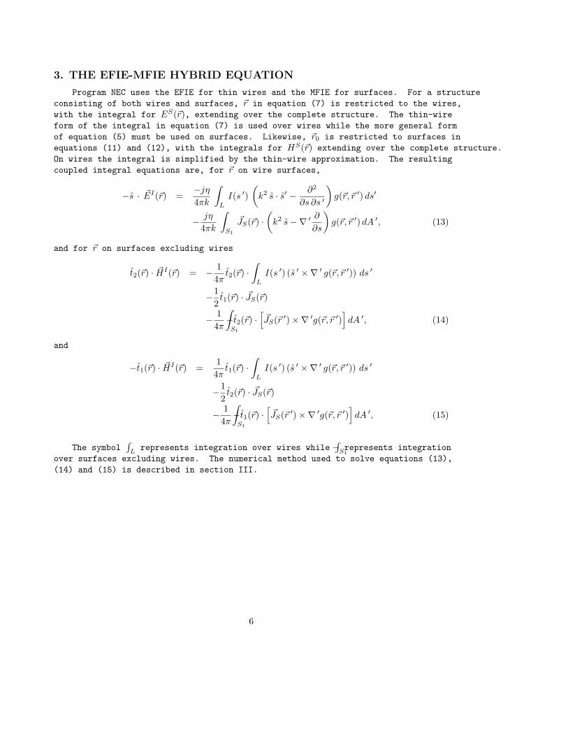
3. THE EFIE-MFIE HYBRID EQUATION

Program NEC uses the EFIE for thin wires and the MFIE for surfaces. For a structure

consisting of both wires and surfaces, ~r in equation (7) is restricted to the wires,

with the integral for ES(~r), extending over the complete structure. The thin-wire

form of the integral in equation (7) is used over wires while the more general form

of equation (5) must be used on surfaces. Likewise, ~r0 is restricted to surfaces in

equations (11) and (12), with the integrals for HS(~r) extending over the complete structure.

On wires the integral is simplified by the thin-wire approximation. The resulting

coupled integral equations are, for ~r on wire surfaces,

−s · ~EI(~r) =−jη

4πk

∫

L

I(s ′)

(

k2 s · s′ − ∂2

∂s ∂s ′

)

g(~r, ~r ′) ds′

− jη

4πk

∫

S1

~JS(~r) ·(

k2 s −∇ ′∂

∂s

)

g(~r, ~r ′) dA ′, (13)

and for ~r on surfaces excluding wires

t2(~r) · ~HI(~r) = − 1

4πt2(~r) ·

∫

L

I(s ′) (s ′ ×∇ ′ g(~r, ~r ′)) ds ′

−1

2t1(~r) · ~JS(~r)

− 1

4π

∫

S1

−t2(~r) ·[

~JS(~r ′) ×∇ ′g(~r, ~r ′)]

dA ′, (14)

and

−t1(~r) · ~HI(~r) =1

4πt1(~r) ·

∫

L

I(s ′) (s ′ ×∇ ′ g(~r, ~r ′)) ds ′

−1

2t2(~r) · ~JS(~r)

− 1

4π

∫

S1

−t1(~r) ·[

~JS(~r ′) ×∇ ′g(~r, ~r ′)]

dA ′, (15)

The symbol∫

Lrepresents integration over wires while

∫

S1− represents integration

over surfaces excluding wires. The numerical method used to solve equations (13),

(14) and (15) is described in section III.

6

Section III - Numerical SolutionThe integral equations (l3), (l4), and (l5) are solved numerically in NEC by a

form of the method of moments. An excellent general introduction to the method of

moments can be found in R. F. Harrington’s book, Field Computation by Moment Methods

(ref. l3). A brief outline of the method follows.

The method of moments applies to a general linear-operator equation,

Lf = e, (16)

where f is an unknown response, e is a known excitation, and L is a linear operator

(an integral operator in the present case). The unknown function f may be expanded

in a sum of basis functions, fj, as

f =

N∑

j=1

αjfj . (17)

A set of equations for the coefficients αj are then obtained by taking the inner product

or equation (16) with a set of weighting functions |wi|,

< wi, Lf > = < wi, e > i = 1, ...N (18)

Due to the linearity of L equation (17) substituted for f yields,

N∑

j−1

αj < wi, Lf > = < wi, e >, i = 1, ...N. (19)

This equation can be written in matrix notation as

[G] [A] = [E] ,

where

Gij = < wi, Lfj >,

Aj = αj ,

Ei = < wi, e > .

The solution is then

[A] = [G]−1

[E] .

For the solution of equations (13), (l4), and (l5), the inner product is derived

as

< f, g >=

∫

S

f(~r)g(~r)dA,

where the integration is over the structure surface. Various choices are possible

for the weighting function wi and basis functions fj. When wi = fi, the procedure

7

is known as Galerkin’s method. In NEC the basis functions are different, wi being

chosen as a set of delta functions

wi(~r) = δ(~r − ~ri),

with ~ri a set of points on the conducting surface. The result is a point sampling

of the integral equations known as the collocation method of solution. Wires are divided

into short straight segments with a sample point at the center of each segment while

surfaces are approximated by a set of flat patches or facets with a sample point at

the center of each patch.

The choice of basis functions is very important for an efficient and accurate solution.

In NEC the support of fi is restricted to a localized subsection of the surface near

~ri. This choice simplifies the evaluation of the inner-product integral and ensures

that the matrix G will be well conditioned. For finite N, the sum of fj cannot exactly

equal a general current distribution, so the functions fi should be chosen as close

as possible to the actual current distribution. Because of the nature of the integral-equation

kernels, the choice of basis function is much more critical on wires than on surfaces.

The functions used in NEC are explained in the following sections.

l. CURRENT EXPANSION ON WIRES

Wires in NEC are modeled by short straight segments with the current on each segment

represented by three terms - a constant, a sine, and a cosine. This expansion was

first used by Yeh and Mei (ref. 14) and has been shown to provide rapid solution convergence

(ref. 15 and 16). It has the added advantage that the fields of the sinusoidal currents

are easily evaluated in closed form. The amplitudes of the constant, sine and cosine

terms are related such that their sum satisfies physical conditions on the local behavior

of current and charge at the segment ends. This differs from AMP where the current

was extrapolated to the centers of the adjacent segments, resulting in discontinuities

in current and charge at the segment ends. Matching at the segment ends improves the

solution accuracy, especially at the multiple-wire junctions of unequal length segments

where AMP extrapolated to an average length segment, often with inaccurate results.

The total current on segment number j in NEC has the form

Ij(s) = Aj + Bj sin k(s − sj) + Cj cos k(s − sj), (20)

|s − sj | < ∆j/2,

where sj is the value of s at the center of segment i and ∆j is the length of segment

j. Of the three unknown constants Aj, Bj, and Cj, two are eliminated by local conditions

on the current leaving one constant, related to the current amplitude, to be determined

by the matrix equation. The local conditions are applied to the current and to the

linear charge density, q, which is related to the current by the equation of continuity

∂I

∂s= −jωq. (21)

8

At a junction of two segments with uniform radius, the obvious conditions are that

the current and charge are continuous at the junction. At a junction of two or more

segments with unequal radii, the continuity or current is generalized to Kirchoff’s

current law that the sum of currents into the junction is zero. The total charge in

the vicinity of the junction is assumed to distribute itself on individual wires according

to the wire radii, neglecting local coupling effects. T. T. Wu and R. W. P. King (ref.

l7) have derived a condition that the linear charge density on a wire at a junction,

and hence ∂I/∂s, is determined by

∂I(s)

∂s

∣

∣

∣

∣

∣

s at junction

=Q

ln(

2ka

)

− γ, (22)

where a is the wire radius,

k = 2π/λ,

γ = 0.5772 (Euler’s constant).

Q is related to the total charge in the vicinity of the junction and is constant for

all wires at the junction.

At a free wire end, the current may be assumed to go to zero. On a wire of finite

radius, however, the current can flow onto the end cap and hence be nonzero at the

wire end. In one study of this effect, a condition relaxing the current at the wire

end to the current derivative was derived (ref. 18). For a wire or radius a, this

condition is

I(s)

∣

∣

∣

∣

∣

s at end

=−s · nc

k

J1(ka)

J0(ka)

∂I(s)

∂s

∣

∣

∣

∣

∣

s at endwhere J0 and J1 are Bessel functions of order 0 and l. The unit vector nc is normal

to the end cap. Hence, s·nc is +l if the reference direction, ~s, is toward the end,

and -1 if s is away from the end.

Thus, for each segment two equations are obtained from the two ends

Ij(sj ± ∆j/2) =±1

k

J1(kaj)

J0(kaj)

∂I(s)

∂s

∣

∣

∣

∣

∣

s=sj±∆j/2

(23)

at free ends, and

∂I(s)

∂s

∣

∣

∣

∣

∣

s=sj±∆j/2

=Q±

1

ln(

2ka

)

− γ, (24)

at junctions. Two additional unknowns Q−

j and Q+j are associated with the junctions

but can be eliminated by Kirchoff’s current equation at each junction. The boundary-condition

equations provide the additional equation- per-segment to completely determine the

current function of equation (20) for every segment.

To apply these conditions, the current is expanded in a sum of basis functions

chosen so that they satisfy the local conditions on current and charge in any linear

combination. A typical set of basis functions and their sum on a four segment wire

are shown in figure 1. For a general segment i in figure 2, the i-th basis function

has a peak on segment i and extends onto every segment connected to i, going to zero

with zero derivative at the outer ends of the connected segments.

9

1 2 3 4

I

Figure l. Current Basis Functions and Sum on a Four Segment Wire.

N+b

b

b

4

3

2

j = 1

12

N−

2

j = 1

i

Figure 2. Segments Covered by the i-th Basis Function.

The general definition of the i-th basis function is given below. For the junction

and end conditions described above, the following definitions apply for the factors

in the segment end conditions:

a−

i = a+i =

[

ln

(

2

kai

)

− γ

]

, (25)

and

Xi = J1(kai)/J0(kai).

The condition of zero current at a free end may be obtained by setting Xi to zero.

The portion of the i-th basis function on segment i is then

f0i (s) = A0

i + B0i sin k(s − si) + C0

i cos k(s − si) (26)

10

|s − si| < ∆i/2.

If N− 6= 0 and N+ 6= 0, end conditions are

∂

∂sf0

i (s)

∣

∣

∣

∣

∣

s=si−∆i/2

= a−

i Q−

i , (27)

∂

∂sf0

i (s)

∣

∣

∣

∣

∣

s=si+∆i/2

= a+i Q+

i . (28)

If N− = 0 and N+ 6= 0, end conditions are

f0i (si − ∆i/2) =

1

kXi

∂

∂sf0

i (s)

∣

∣

∣

∣

∣

s=si−∆i/2

(29)

∂

∂sf0

i (s)

∣

∣

∣

∣

∣

s=si+∆i/2

= a+i Q+

i . (30)

If N− 6= 0 and N+ = 0, end conditions are

∂

∂sf0

i (s)

∣

∣

∣

∣

∣

s=si−∆i/2

= a−

i Q−

i , (31)

f0i (si + ∆i/2) =

−1

kXi

∂

∂sf0

i (s)

∣

∣

∣

∣

∣

s=si+∆i/2

(32)

Over segments connected to end 1 of segment 1, the i-th basis function is

f−

j (s) = A−

j + B−

j sin k(s − sj) + C−

j cos k(s − sj) (33)

|s − sj | < ∆j/2 j = 1, ..., N−.

End conditions are

f−

j (aj − ∆j/2) = 0, (34)

∂

∂sf−

j (s)

∣

∣

∣

∣

∣

s=sj−∆j/2

= 0, (35)

∂

∂sf−

j (s)

∣

∣

∣

∣

∣

s=sj−∆j/2

= a+j Q−

j . (36)

Over segments connected to end 2 of segment i, the i-th basis function is

f+j (s) = A+

j + B+j sin k(s − sj) + C+

j cos k(s − sj) (37)

11

|s − sj | < ∆j/2 j = 1, ..., N+.

End conditions are

∂

∂sf+

j (s)

∣

∣

∣

∣

∣

s=sj−∆j/2

= a−

j Q+j . (38)

f+j (sj + ∆j/2) = 0, (39)

∂

∂sf+

j (s)

∣

∣

∣

∣

∣

s=sj+∆j/2

= 0, (40)

Equations (26), (33) and (37), defining the complete basis function, involve 3(N−+N++1) unknown constants. Of these, 3(N−+N+)+2 unknowns are eliminated by the

end conditions in terms of Q−

i and Q+i which can then be determined from the two Kirchoff’s

current equations:

N−

∑

j=1

f−

j (sj + ∆j/2) = f0i (si − ∆i/2), and (41)

N+

∑

j=1

f+j (sj − ∆j/2) = f0

i (si + ∆i/2). (42)

The complete basis function is then defined in terms of one unknown constant. In

this case A0i was set to −1 since the function amplitude is arbitrary, being determined

by the boundary condition equations. The final result is given below:

A−

j =a+

j Q−

i

sin k∆j, (43)

B−

j =a+

j Q−

i

2 cos k∆j/2, (44)

C−

j =−a+

j Q−

i

2 sin k∆j/2, (45)

A+j =

−a−

j Q+i

sin k∆j, (46)

B+j =

a−

j Q+i

2 cos k∆j/2, (47)

12

C+j =

a−

j Q+i

2 sin k∆j/2, (48)

For N− 6= 0 and N+ 6= 0,A0

i = −1, (49)

B0i =

(

a−

i Q−

i + a+i Q+

i

)

sin k∆i/2

sin k∆i, (50)

C0i =

(

a−

i Q−

i − a+i Q+

i

)

cos k∆i/2

sin k∆i, (51)

Q−

i =a+

i (1 − cos k∆i) − P+i sin k∆i

(

P−

i P+i + a−

i a+i

)

sin k∆i +

(

P−

i a+i − P+

i a−

i

)

cos k∆i

, (52)

Q+i =

a−

i (cos k∆i − 1) − P−

i sin k∆i(

P−

i P+i + a−

i a+i

)

sin k∆i +

(

P−

i a+i − P+

i a−

i

)

cos k∆i

. (53)

For N− = 0 and N+ 6= 0,A0

i = −1, (54)

B0i =

sin k∆i/2

cos k∆i − Xi sin k∆i+ a−

i Q+i

cos k∆i/2 − Xi sin k∆i/2

cos k∆i − Xi sin k∆i, (55)

C0i =

cos k∆i/2

cos k∆i − Xi sin k∆i+ a+

i Q+i

sin k∆i/2 − Xi cos k∆i/2

cos k∆i − Xi sin k∆i, (56)

Q+i =

cos k∆i − 1 − Xisin k∆i(

a+i + XiP

+i

)

sin k∆i +

(

a+i Xi − P+

i

)

cos k∆i

. (57)

For N− 6= 0 and N+ = 0,A0

i = −1, (58)

B0i =

− sin k∆i/2

cos k∆i − Xi sin k∆i+ a−

i Q−

i

cos k∆i/2 − Xi sin k∆i/2

cos k∆i − Xi sin k∆i, (59)

C0i =

cos k∆i/2

cos k∆i − Xi sin k∆i− a−

i Q−

i

sin k∆i/2 + Xi cos k∆i/2

cos k∆i − Xi sin k∆i, (60)

13

Q−

i =1 − cos k∆i + Xisin k∆i

(

a−

i − XiP−

i

)

sin k∆i +

(

P−

i + Xia−

i

)

cos k∆i

. (61)

For all cases,

P−

i =

N−

∑

j=1

(

1 − cos k∆j

sin k∆j

)

a+j , (62)

P+i =

N+

∑

j=1

(

cos k∆j − 1

sin k∆j

)

a−

j , (63)

where the sum for P−

i is over segments connected to end l of segment i, and the sum

for P+i is over segments connected to end 2. If N− = N+ = 0, the complete basis

function is

f0i =

cos k(s − si)

cos k∆i/2 − Xi sin k∆i/2− 1. (64)

When a segment end is connected to a ground plane or to a surface modeled with

the MFIE, the end condition on both the total current and the last basis function is

∂

∂sIj(s)

∣

∣

∣

∣

∣

s=sj±∆j/2

= 0,

replacing the zero current condition at a free end. This condition does not require

a separate treatment, however, but is obtained by computing the last basis function

as if the last segment is connected to its image segment on the other side of the surface.

It should be noted that in AMP, the basis function fi has unit value at the center

of segment i and zero value at the centers of connected segments although it does extend

onto the connected segments. As a result, the amplitude of fi is the total current

at the center of segment i. This is not true in NEC so the current at the center of

segment i must be computed by summing the contributions of all basis functions extending

onto segment i.

2. CURRENT EXPANSIONS ON SURFACES

Surfaces on which the MFIE is used are modeled by small flat patches. The surface

current on each patch is expanded in a set of pulse functions except in the region

of wire connection, as will be described later. The pulse function expansion for Np

patches is

~Js(~r) =

Np∑

j=1

(

J1j t1j + J2j t2j

)

Vj(~r), (65)

where

t1j = t1(~rj),

14

t2j = t2(~rj),

~rj = position of the center of patch number j,

Vj(~r) = 1 for ~r on patch j and 0 otherwise.

The constants J1j and J2j, representing average surface-current density over the

patch, are determined by the solution of the linear system of equations derived from

the integral equations. The integrals for fields due to the pulse basis functions,

are evaluated numerically in a single step so that for integration, the pulses could

be reduced to delta functions at the patch centers. That this simple approximation

of the current yields good accuracy is one of the advantages of the MFIE for surfaces.

A more realistic representation of the surface current is needed however, in the

region where a wire connects to the surface. The treatment used in NEC, affecting

the four coplanar patches about the connection point is quite similar to that used

by Albertsen et al. (ref. 9). In the region of the wire connection, the surface current

contains a singular component due to the current flowing from the wire onto the surface.

The total surface current should satisfy the condition,

∇s · ~Js(x, y) = J0(x, y) + I0 δ(x, y),

where the local coordinates x and y are defined in figure 3, ∇s denotes surface divergence,

J0(x, y) is a continuous function in the region ABCD, and I0 is the current at the base

of the wire flowing onto the surface. One expansion which meets this requirement is

~Js(x, y) = I0~f(x, y) +

4∑

j=1

gj(x, y)( ~Jj − I0~fj), (66)

where

~f(x, y) =xx + yy

2π(x2 + y2),

~Jj = ~Js(xj , yj),

~fj = ~f(xj , yj), and

(xj , yj) = (x, y) at the center of patch j. The interpolation functions gj(x, y) are chosen

such that: gj(x, y) is differentiable on ABCD; gj(xi, yi) = δij; and∑4

j=1 gj(x, y) = 1.The specific functions used in NEC are as follows:

g1(x, y) =1

4d2(d + x)(d + y)

g2(x, y) =1

4d2(d − x)(d + y)

g3(x, y) =1

4d2(d − x)(d − y)

g4(x, y) =1

4d2(d + x)(d − y)

15

~x

~y

d

d

b 1

b

4

b3

b2

A

B

C

D

Figure 3. Detail of the connection of a wire to a surface.

Equation (66) is used when computing the electric field at the center of the connected

wire segment due to the surface current on the four surrounding patches. In computing

the field on any other segments or on any patches, the pulse-function form is used

for all patches including those at the connection point. This saves integration time

and is sufficiently accurate for the greatest source to observation-point separations

involved.

16

3. EVALUATION OF THE FIELDS

The current on each wire segment has the form

Ii(s) = Ai + Bi sin k(s − si) + Ci cos k(s − si) (67)

|s − si| < ∆i/2,

where k = ω√

µ0ǫ0 and ∆i is the segment length. The solution requires the evaluation

of the electric field at each segment due to this current. Three approximations or

the integral equation kernel are used - a thin-wire form for most cases, an extended

thin-wire form for thick wires, and a current element approximation for large interaction

distances. In each case the evaluation of the field is greatly simplified by the use

of formulas for the fields of the constant and sinusoidal current components.

The accuracy of the thin-wire approximation for a wire of radius a and length ∆depends on ka and ∆/a. Studies have shown that the thin-wire approximation leads

to errors of less than 1%, for ∆/a greater than 8 (ref. ll). Furthermore, in the

numerical solution of the EFIE, the wire is divided into segments less than about 0.1λin length to obtain an adequate representation of current distribution thus restricting

ka to less than about 0.08. The extended thin-wire approximation is applicable to

shorter and thicker segments, resulting in errors less than 1%, for ∆/a greater than

2.

For the thin-wire kernel, the source current is approximated by a filament on the

segment axis while the observation point is on the surface of the observation segment.

The fields are evaluated with the source segment on the axis of a local cylindrical-coordinate

system as illustrated in Figure 4.

~x

~y

~z

b P

z

ρ

r0

ρ

z1

z2

z ′

Figure 4. Current-Filament Geometry for the Thin-Wire Kernel.

17

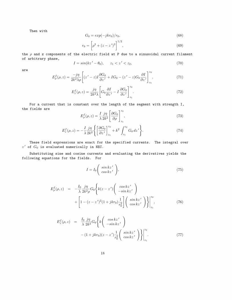
Then with

G0 = exp(−jkr0)/r0, (68)

r0 =

[

ρ2 + (z − z ′)2]1/2

, (69)

the ρ and z components of the electric field at P due to a sinusoidal current filament

of arbitrary phase,

I = sin(kz ′ − θ0), z1 < z ′ < z2, (70)

are

Efρ (ρ, z) =

−jη

2k2λρ

[

(z ′ − z)I∂G0

∂z ′+ IG0 − (z ′ − z)G0

∂I

∂z ′

]z2

z1

, (71)

Efz (ρ, z) =

jη

2k2λ

[

G0∂I

∂z ′− I

∂G0

∂z ′

]z2

z1

. (72)

For a current that is constant over the length of the segment with strength I,

the fields are

Efρ (ρ, z) =

I

λ

jη

2k2

[

∂G0

∂ρ

]z2

z1

, (73)

Efz (ρ, z) = − I

λ

jη

2k2

[

∂G0

∂z ′

]z2

z1

+ k2

∫ z2

z1

G0 dz ′

. (74)

These field expressions are exact for the specified currents. The integral over

z ′ of G0 is evaluated numerically in NEC.

Substituting sine and cosine currents and evaluating the derivatives yields the

following equations for the fields. For

I = I0

(

sin kz ′

cos kz ′

)

, (75)

Efρ (ρ, z) = −I0

λ

jη

2k2ρG0

k(z − z ′)

(

cos kz ′

−sin kz ′

)

+

[

1 − (z − z ′)2(1 + jkr0)1

r20

](

sin kz ′

cos kz ′

)∣

∣

∣

∣

∣

z2

z1

, (76)

Efz (ρ, z) =

I0

λ

jη

2k2G0

k

(

cos kz ′

−sin kz ′

)

− (1 + jkr0)(z − z ′)1

r20

(

sin kz ′

cos kz ′

)∣

∣

∣

∣

∣

z2

z1

. (77)

18

For a constant current of strength I0,

Efρ (ρ, z) = −I0

λ

jηρ

2k2

[

(1 + jkr0)G0

r20

]z2

z1

, (78)

Efρ (ρ, z) = −I0

λ

jηρ

2k2

[

(1 + jkr0)(z − z ′)G0

r20

]z2

z1

+ k2

∫ z2

z1

G0dz ′

. (79)

Despite the seemingly crude approximation, the thin-wire kernel does accurately

represent the effect of wire radius for wires that are sufficiently thin. The accuracy

range was studied by Poggio and Adams (ref. ll) where an extended thin-wire kernel

was developed for wires that are too thick for the thin-wire approximation.

The derivation of the extended thin-wire kernel starts with the current on the

surface of the source segment with surface density,

J(z ′) = I(z ′)/(2πa),

where a is the radius of the source segment. The geometry for evaluation of the fields

is shown in figure 5. A current filament of strength Idφ/(2π) is integrated over Φwith

ρ ′ = [ρ2 + a2 − 2aρ cosΦ]1/2, (80)

r = [(ρ ′)2 + (z − z ′)2]1/2. (81)

Thus, the z component of the field of the current tube is

Etz(ρ, z) =

1

2π

∫ 2π

0

Efz (ρ ′, z) dΦ. (82)

~x

~y

~z

b P

z

ρ

ρ0

a

z1

z2

z ′

r0

r

b

Figure 5. Current geometry for the extended thin-wire kernel.

19

For the ρ component of field, the change in the direction of β ′ must be considered.

The field in the direction β is

Etz(ρ, z) =

1

2π

∫ 2π

0

Efρ (ρ ′, z)(β · β ′) dΦ, (83)

where

β · β ′ =ρ − a cosΦ

ρ ′=

∂ρ ′

∂ρ

The integrals over Φ in equations (82) and (83) cannot be evaluated in closed form.

Roggio and Adams, however, have evaluated them as a series in powers of a2 (ref. ll).

The first term in the series gives the thin-wire kernel. For the extended thin-wire

kernel, the second term involving a2 is retained with terms of order a4 neglected.

As with the thin-wire kernel, the field observation point is on the segment surface.

Hence, when evaluating the field on the source segment, ρ = a.

The field equations with the extended thin-wire approximation are given below.

For a sinusoidal current of equation (70),

Eρ(ρ, z) =−jη

2k2λρ

[

(z ′ − z)I∂G2

∂z ′+ IG2 − (z ′ − z)G2

∂I

∂z ′

]z2

z1

, (84)

Ez(ρ, z) =jη

2k2λ

[

G1∂I

∂z ′− I

∂G1

∂z ′

]z2

z1

, (85)

For a constant current of strength I0,

Eρ(ρ, z) =I

λ

jn

2k2

[

∂G1

∂ρ

]z2

z1

, (86)

Ez(ρ, z) = − I

λ

jn

2k2

[

∂G1

∂z ′

]z2

z1

+ k2

[

1 − (ka)2

4

]

∫ z2

z1

G0 dz ′ − (ka)2

4

[

∂G0

∂z ′

]z2

z1

. (87)

20

The term G1 is the series approximation of

Gt1 =

1

2π

∫ 2π

0

GdΦ, (88)

where

G = exp(−jkr)/r.

Neglecting terms of order a4,

G1 = G0

1 − a2

2r20

(1 + jkr0) +a2ρ2

4r20

[

3(1 + jkr) − k2r20

]

, (89)

∂G1

∂z ′=

(z − z ′)

r20

G0

(1 + jkr0) −a2

2r20

[

3(1 + jkr) − k2r20

]

−a2ρ2

4r40

[

jk3r30 + 6k2r2

0 − 15(1 + jkr0)

]

, (90)

∂G1

∂ρ= −ρG0

r20

(1 + jkr0) −a2

r20

[

3(1 + jkr) − k2r20

]

−a2ρ2

4r40

[

jk3r30 + 6k2r2

0 − 15(1 + jkr0)

]

, (91)

The term G2 is the series approximation of

Gt2 =

1

2π

∫ 2π

0

ρ − a cosΦ

ρ ′2GdΦ, (92)

To order a2,

G1 =G0

ρ

1 +a2ρ2

4r20

[

3(1 + jkr) − k2r20

]

, (93)

∂G1

∂z ′=

(z − z ′)

ρr20

G0

(1 + jkr0) −a2ρ2

4r40

[

jk3r30 + 6k2r2

0 − 15(1 + jkr0)

]

. (94)

Equation (86) makes use of the relation

(β · β ′)∂G

∂ρ ′=

∂G

∂ρ ′

∂ρ ′

∂ρ=

∂G

∂ρ, (95)

while equation (87), follows from

G1 =

[

1 − (ka)2

4− a2

4

∂2

∂z ′2

]

G0. (96)

21

When the observation point is within the wire (ρ < a), a series expansion in ρrather than a is used for G0 and G2. For G1 this simply involves interchanging ρand a in equations (89) and (90). Then for ρ < a, with

ra =

[

a2 + (z − z ′)2]1/2

, (97)

Ga = exp(−jkra)/ra, (98)

the expressions for G1, G2 and their derivatives are

G1 = Ga

1 − ρ2

2r2a

(1 + jkra) +a2ρ2

4r4a

[

3(1 + jkra) − k2r2a

]

, (99)

∂G1

∂z ′=

(z − z ′)

r2a

Ga

(1 + jkra) − ρ2

2r2a

[

3(1 + jkra) − k2r2a

]

−a2ρ2

4r4a

[

jk3r3a + 6k2r2

a − 15(1 + jkra)

]

, (100)

∂G1

∂ρ= −ρGa

r2a

(1 + jkra) − a2

2r2a

[

3(1 + jkra) − k2r2a

]

, (101)

G2 = − ρ

2r2a

Ga(1 + jkra), (102)

∂G2

∂z ′= − (z − z ′)ρ

2r4a

Ga

[

3(1 + jkra) − k2r2a

]

(103)

Special treatment of bends in wires is required when the extended thin wire kernel

is used. The problem stems from the cancellation of terms evaluated at z1 and z2 in

the field equations when segments are part of a continuous wire. The current expansion

in NEC results in a current having a continuous value and derivative along a wire without

junctions. This ensures that for two adjacent segments on a straight wire, the contributions

to the z component of electric field at z2, of the first segment exactly cancel the

contributions from z1 representing the same point, for the second segment. For a straight

wire or several segments, the only contributions for Ez with either the thin-wire or

extended thin-wire kernel come from the two wire ends and the integral of G0 along

the wire. For the ρ component of field or either component at a bend, while there

is not complete cancellation, there may be partial cancellation of large end contributions.

The cancellation of end terms makes necessary a consistent treatment of the current

on both sides of a bend for accurate evaluation of the field. This is easily accomplished

with the thin-wire kernel since the current filament on the wire axis is physically

continuous around a bend. However, the current tube assumed for the extended thin-wire

kernel cannot be continuous around its complete circumference at a bend. This was

found to reduce the solution accuracy when the extended thin-wire kernel was used for

bent wires.

22

To avoid this problem in NEC, the thin-wire form or the end terms in equation (71)

through (74) is always used at a bend or change in radius. The extended thin-wire

kernel is used only at segment ends where two parallel segments join, or at free ends.

The switch from extended thin-wire to the thin-wire form is made from one end of a

segment to the other rather than between segments where the cancellation of terms is

critical.

When segments are separated by a large distance, the interaction may be computed

with sufficient accuracy by treating the segment current as an infinitesimal current

element at the segment center. In spherical coordinates with the segment at the origin

along the θ = 0 axis, the electric field is

Er(r, θ) =Mη

2πr2exp(−jkr)

(

1 − j

kr

)

cosθ,

Eθ(r, θ) =Mη

2πr2exp(−jkr)

(

1 + jkr − j

kr

)

sinθ.

The dipole moment M for a constant current I on a segment of length ∆i is

M = I∆i.

For a current I cos[k(s − si)] with |s − si| < ∆i/2,

M =2I

ksin (k∆i/2),

while for a current I sin[k(s − si)],M = 0.

Use of this approximation saves a significant amount of time in evaluating the interaction

matrix elements for large structures. The minimum interaction distance at which it

is used is selected by the user in NEC. A default distance of one wavelength is set,

however. For each of the three methods of computing the field at a segment due to

the current on another segment, the field is evaluated on the surface of the observation

segment. Rather than choosing a fixed point on the segment surface, the field is evaluated

at the cylindrical coordinates ρ ′, z with the source segment at the origin. If the

center point on the axis of the observation segment is at ρ, z, then

ρ ′ =

[

ρ2 + a20

]1/2

,

where a0 is the radius of the observation segment. Also, the component of Eρ tangent

to the observation segment is computed as

~Eρ · s = (ρ · s) ρ

ρ ′Eρ.

inclusion of the factor ρ/ρ ′, which is the cosine of the angle between β and β ′, is

necessary for accurate results at bends in thick wires.

23

4. THE MATRIX EQUATION FOR CURRENT

For a structure having Ns wire segments and Np patches, the order of the matrix

in equation (l9) is N = Ns + 2Np. In NEC the wire segment equations occur first

in the linear system so that, in terms of submatrices, the equation has the form

A B

C D

Iw

Ip

=

Ew

Hp

,

With equations derived from equation (14) in odd numbered rows in the lower set and

equation (l5) in even rows. Iw is then the column vector of segment basis function

amplitudes, and Ip is the patch-current amplitudes (J1j , J2j , j = 1, ..., Np) The elements

of Ew are the left-hand side of equation (13) evaluated at segment centers, while

Hp contains, alternately, the left-hand sides of equations (l4) and (15) evaluated

at patch centers.

A matrix element Aij, in submatrix A, represents the electric field at the center

of segment i due to the j-th segment basis function, centered on segment j. A matrix

element Dij in submatrix D represents a tangential magnetic fie1d component at patch

k due to a surface-current pulse on patch l where

k = Int[(i − 1)/2] + 1,

l = Int[(j − 1)/2] + 1,

and Int[ ] indicates truncation. The source pulse is in the direction t1 when j is odd,

and direction t2 when j is even. When k = l the contribution of the surface integral

is zero since the vector product is zero on the flat patch surface, although a ground

image may produce a contribution. However, for k = l, there is a contribution of

± 1/2 from the coefficient of ~Js(~r) equation (l4) or (l5). Matrix elements in submatrices

B and C represent electric fields due to surface-current pulses and magnetic fields

due to segment basis functions, respectively. These present no special problems since

the source and observation points are always separated.

24

5. SOLUTION OF THE MATRIX EQUATION

The matrix equation,

[G][I] = [E], (104)

is solved in NEC by Gauss elimination (ref. 19). The basic step is factorization of

the matrix G into the product of an upper triangular matrix U and a lower triangle

matrix L where

[G] = [L][U ].

The matrix equation is then

[L][U ][I] = [E], (105)

from which the solution, I, is computed in two steps as

[L][F ] = [E], (106)

and

[U ][I] = [F ]. (107)

Equation (l06) is first solved for F by forward substitution, and equation (107) is

then solved for I by backward substitution.

The major computational effort is factoring G into L and U. This takes approximately

1/3N3 multiplication steps for a matrix of order N compared to N3 for inversion of

G by the Gauss-Jordan method. Solution of equations may be reduced substantially by

making use of symmetries or the structure either symmetry about a plane, or symmetry

under rotation.

In rotational symmetry, a structure having M sectors is unchanged when rotated

by any multiple of 360/M degrees. If the equations for all segments and patches in

the first sector are numbered first and followed by successive sectors in the same

order, the matrix equation can be expanded in submatrices in the form

A1 A2 A3 . . . AM−1 AM

AM A1 A2 . . . AM−2 AM−1

AM−1 AM A1 . . . AM−3 AM−2

. . .

. . .

. . .

. . .A2 A3 A4 AM A1

I1

I2

I3

.

.

.

.IM

=

E1

E2

E3

.

.

.

.EM

(108)

25

If there are Nc equations in each sector, Ei and Ii are Nc element column vectors

of the excitations and currents in sector i. Ai is a submatrix of order Nc containing

the interaction fields in sector 1 due to currents in sector i. Due to symmetry, this

is the same as the fields in sector k due to currents in sector i + k, resulting in

the repetition pattern shown. Thus only matrix elements in the first row of submatrices

need be computed reducing the time to fill the matrix by a factor of l/M.

The time to solve the matrix equation can also be reduced by expanding the excitation

subvectors in a discrete Fourier series as

Ei =

M∑

k=1

Sik Ek i = 1, ...,M, (109)

Ei =1

M

M∑

k=1

S∗

ik Ek i = 1, ...,M, (110)

where

Sik = exp[j2π(i − 1)(k − 1)/M ] (111)

j =√−1, and * indicates the conjugate of the complex number. Examining a component

in the expansion,

E =

S1k Ek

S2k Ek

S3k Ek

.

.

.SMk Ek

, (112)

it is seen that the excitation differs from sector to sector only by a uniform phase

shift. This excitation of a rotationally symmetric structure results in a solution

having the same form as the excitation, i.e.,

I =

S1k Ik

S2k Ik

S3k Ik

.

.

.SMk Ik

, (113)

It can be shown that this relation between solution and excitation holds for any matrix

having the form of that in equation (108). Substituting these components of E and

I into equation (108) yields the following matrix equation of order Nc relating Ik

to Ek;

[S1k A1 + S1k A1 + ... + SMk AM ][Ik] = S1k[Ek]. (114)

The solution for the total excitation is then obtained by an inverse transformation,

Ii =M∑

k=1

Sik Ik i = 1, ...,M. (115)

26

The solution procedure, then, is first to compute the M submatrices Ai and Fourier-transform

these to obtain

Ai =

M∑

k=1

Sik Ak i = 1, ...,M. (116)

The matrices Ai, of order Nc, are then each factored into upper and lower triangular

matrices by the Gauss elimination method. For each excitation vector, the transformed

subvectors are then computed by equation (110) and the transformed current subvectors

are obtained by solving the M equations

[Ai] [Ii] = [Ei]. (117)

The total solution is then given by equation (ll5).

The same procedure can be used for structures that have planes of symmetry. The

Fourier transform is then replaced by even and odd excitations about each symmetry

plane. All equations remain the same with the exception that the matrix S with elements

Sij, given by equation (lll), is replaced by the following matrices:

For one plane of symmetry,

S =

[

1 11 −1

]

;

For two orthogonal planes of symmetry,

S =

1 1 1 11 −1 1 −11 1 −1 −11 −1 −1 1

;

and for three orthogonal symmetry planes,

S =

1 1 1 1 1 1 1 11 −1 1 −1 1 −1 1 −11 1 −1 −1 1 1 −1 −11 −1 −1 1 1 −1 −1 11 1 1 1 −1 −1 −1 −11 −1 1 −1 −1 1 −1 11 −1 1 −1 −1 1 −1 11 1 −1 −1 −1 −1 1 11 −1 −1 1 −1 1 1 −1

;

For either rotational or plane symmetry, the procedure requires factoring of M matrices

of order Nc rather than one matrix of order MNc. Each excitation then requires the

solution of the M matrix equations. Since the time for factoring is approximately

proportional to the cube or the matrix order and the time for solution is proportional

to the square of the order, the symmetry results in a reduction of factor time by M−2

and in solution time by M−1. The time to compute the transforms is generally small

compared to the time for matrix operations since it is proportional to a lower power

27

of Nc. Symmetry also reduces the number of locations required for matrix storage

by M−1 since on1y the first row of submatrices need be stored. The transformed matrices,

Ai, can replace the matrices Ai as they are computed.

NEC includes a provision to generate and factor an interaction matrix and save

the result in a file. A later run, using the file, may add to the structure and solve

the complete model without unnecessary repetition of calculations. This procedure

is called the Numerical Green’s Function (NGF) option since the effect is as if the

free space Green’s Function in NEC were replaced by the Green’s function for the structure

in the file. The NGF is particularly useful for a large structure, such as a ship,

on which various antennas will be added or modified. It also permits taking advantage

of partial symmetry since a NGF file may be written for the symmetric part of a structure,

taking advantage of the symmetry to reduce computation time. Unsymmetric parts can

then be added in a later run.

For the NGF solution the matrix is partitioned as

[

A BC D

] [

I1

I2

]

=

[

E1

E2

]

.

Where A is the interaction matrix for the initial structure, D is the matrix for the

added structure, and B and C represent mutual interactions. The current is computed

as

I2 = [D − CA−1B]−1[E2 − CA−1E1],

I1 = A−1E1 − A−1BI2.

after the factored matrix A has been read from the NGF fi1e along with other necessary

data.

Electrical connections between the new structure and the old (NGF) structure require

special treatment. If a new wire or patch connects to an old wire the current basis

function for the old wire segment is changed by the modified condition at the junction.

The old basis function is given zero amplitude by adding a new equation having all

zeros except for a one in the column of the old basis function. A new column is added

for the corrected basis function. When a new wire connects to an old patch the patch

must be divided into four new patches to apply the connection condition or equation

(5l). Hence both the current basis function and match point for the old patch are

replaced.

28

Section IV - Effect of Ground Plane

In the integral equation formulation used in NEC, a ground plane changes the solution

in three ways; (l) by modifying the current distribution through near-field interaction;

(2) by changing the field illuminating the structure; and (3) by changing the reradiated

field. Effects (2) and (3) are easily analyzed by plane-wave reflection as a direct

ray and a ray reflected from the ground. The reradiated field is not a plane wave

when it reflects from the ground, but, as can be seen from reciprocity, plane-wave

reflection gives the correct far-zone field. Analysis of the near-field interaction

effect is, however, much more difficult.

In section II, the kernels of the integral equations are free-space Green’s Functions,

representing the E or H field at a point ~r due to an infinitesimal electric current

element at ~r ′. When a ground is present the free space Green’s functions must be replaced

by Green’s functions for the ground problem. The solution for the fields of current

elements in the presence of a ground plane was developed by Arnold Sommerfeld (ref.

20). While this solution has been used directly in integral-equation computer codes,

excessive computation time greatly limits its use. Numerous approximations to the

Sommerfeld solution have been developed that require less time for evaluation but all

have limited applicability.

The NEC code has three options for grounds. The most accurate for lossy grounds

uses the Sommerfeld solution for interaction distances less than one wavelength and

an asymptotic expansion for larger distances. To keep the solution time reasonable,

a grid of values of the Sommerfeld solution is generated and interpolation is used

to find specific values. This method is presently implemented only for wires in NEC

but could be extended to patches. The solution for a perfectly conducting ground is

much simpler since the ground may be replaced by the image of the currents above it.

The third option models a lossy ground by a modified image method using the Fresnel

plane-wave reflection coefficients. While specular reflection does not accurately

describe the behavior of near fields, the approximation has been found to provide useful

results for structures that are not too near to the ground (refs. 21, 22). The attraction

of this method is its simplicity and speed of computation which are the same as for

the image method for perfect ground.

29

1. THE SOMMERFELD/NORTON METHOD

The Sommerfeld/Norton ground option in NEC originated with the code WFLLL2A (ref.

23) which uses numerical evaluation of the Sommerfeld integrals for ground fields when

the interaction distance is small and uses Norton’s asymptotic approximations (ref.

25). For larger distances, since evaluation of the Sommerfeld integrals is very time

consuming, a code, SOMINT, was developed (ref. 25) which uses bivariate interpolation

in a table of precomputed Sommerfeld integral values to obtain the field values needed

for integration over current distributions. This method greatly reduces the required

computation time. NEC uses a similar interpolation method with modifications to allow

wires closer to the air-ground interface and to further reduce computation time. Although

the code WFLLL2A allows wires both above and below the interface, both NEC and SOMINT

are presently restricted to wires on the free-space side. The method used in NEC to

evaluate the field over ground is described below, and the numerical evaluation of

the Sommerfeld integrals to fill the interpolation grid is discussed in Section IV-2.

The electric field above an air-ground interface due to an infinitesimal current

element of strength Il also above the interface, with parameters shown in figure 6,

is given by the following expressions:

EVρ = C1

∂2

∂ρ∂z[G22 − G21 + k2

1 V22], (118)

EVz = C1(

∂2

∂z2+ k2

2)[G22 − G21 + k21 V22], (119)

EHρ = C1cosΦ [

∂2

∂ρ2(G22 − G21 + k2

2V22) + k22(G22 − G21 + U22)], (120)

EHΦ = −C1sinΦ [

1

ρ

∂

∂ρ(G22 − G21 + k2

2V22) + k22(G22 − G21 + U22)], (121)

EHz = C1cosΦ [

∂2

∂z∂ρ(G22 − G21 + k2

1V22)], (122)

C1 =−jωIlµ0

4πk22

, (123)

k21 = ω2µ0ǫ0

(

ǫ1ǫ0

− jσ1

ωǫ0

)

, (124)

k22 = ω2µ0ǫ0, (125)

where the superscript indicates vertical (V) or horizontal (H) current element and

the subscript indicates the cylindrical component of the field vector. The horizontal

current element is along the x-axis.

30

~x

~y

~z

b

z

b

z ′

ρ

Source

Air ǫ0, µ0

Ground ǫ1, µ1, σ1

Φ

Figure 6. Coordinates for Evaluating the Field of a Current Element Over Ground.

G22 and G21 are the free space and image Green’s functions

G22 =exp (−jk2R2)

R2, (126)

G21 =exp (−jk2R1)

R1, (127)

where

R1 =

[

ρ2 + (z + z ′)2]1/2

, (128)

R2 =

[

ρ2 + (z − z ′)2]1/2

, (129)

and U22, and V22 are Sommerfeld integrals involving the zero-th order Bessel function,

J0

U22 = 2

∫ ∞

0

exp[−γ2(z + z ′)]J0(λρ)λ dλ

γ1 + γ2, (130)

V22 = 2

∫ ∞

0

exp[−γ2(z + z ′)]J0(λρ)λ dλ

k21 γ1 + k2

2 γ2, (131)

where

γ1 = (λ2 − k21)

1/2, (132)

γ2 = (λ2 − k22)

1/2. (133)

In NEC we need to compute the fields due to current elements with arbitrary length

and orientation by combining the field components in equations (ll8) through (122)

31

and integrating over current distributions composed of constant, sine, and cosine components.

Direct numerical integration over the segments is difficult due to singularities in

the fields. G22 has a 1/R2 singularity while G21, U22, and V22, each have 1/R1 singularities.

The derivatives in the field expressions result in 1/R3 singularities with a triplet

like behavior in the field components parallel to the current filament. The resulting

cancellation makes accurate numerical integration near the singularity very difficult.

The free-space field has a similar singularity, but as discussed in section III-3,

the integral over a straight filament may be evaluated in closed form for a sinusoidal

current with free-space wavelength and involves only a numerical integration of G22

for a constant current. The dominant singular component of the ground field may be

integrated in the same way. The terms involving G22 in equation (118) through (122)

are, in fact, the field of the current element in free space, and their integral is

obtained from the free-space routines in NEC.

The remaining terms represent the field due to ground and are singular at R1 =0. The singularities in U22 and V22 result from the failure of the integrals in equations

(130) and (131) to converge without the exponential and Bessel functions as ρ and z

+ z’ go to zero. The singular behavior of U22, and V22 as ρ and z + z ’ go to zero

may be found by setting γ1 = γ2 = λ since the dominant contributions to the integrals

for small ρ and z + z’ come from λ much greater than k1 or k2. Here, however, we only

replace γ1 by γ2 and use the integrals

V22 = 2

∫ ∞

0

exp[−γ2(z + z ′)]J0(λρ)λ dλ

γ2(k21 + k2

2)=

2G21

k21 + k2

2

, (134)

U22 = 2

∫ ∞

0

exp[−γ2(z + z ′)]J0(λρ)λ dλ

γ2= G21 (135)

|k1|ρ << 1, |k1|(z + z ′) << 1,

which have the correct singular behavior and can be combined with the G21 terms. The

field components due to ground [equation (108) through (122) without the G22 terms]

may then be written as

GVρ = C1

∂2

∂ρ∂zk21 V ′

22 + C1k21 − k2

2

k21 + k2

2

∂2

∂ρ∂zG21, (136)

GVz = C1

(

∂2

∂z2+ k2

2

)

k21 V ′

22 + C1k21 − k2

2

k21 + k2

2

(

∂2

∂z2+ k2

2

)

G21, (137)

GHρ = C1cosΦ

(

∂2

∂ρ2k22V

′

22 + k22U

′

22

)

− C1cosΦk21 − k2

2

k21 + k2

2

(

∂2

∂ρ2+ k2

2

)

G21, (138)

GHΦ = −C1sinΦ

(

1

ρ

∂

∂ρk22V

′

22 + k22U

′

22

)

+ C1sinΦk21 − k2

2

k21 + k2

2

(

1

ρ

∂

∂ρ+ k2

2

)

G21, (139)

GHz = −cosΦGV

ρ , (140)

U ′

22 = U22 −2k2

2

k21 + k2

2

G21 ,

= 2

∫ ∞

0

[

1

γ1 + γ2− k2

2

γ2(k21 + k2

2)

]

exp[−γ2(z + z ′)]J0(λρ)λ dλ , (141)

32

V ′

22 = V22 −2

k21 + k2

2

G21 ,

= 2

∫ ∞

0

[

1

k21γ1 + k2

2γ2− 1

γ2k21 + k2

2

]

exp[−γ2(z + z ′)]J0(λρ)λ dλ . (142)

In equations (136) through (140) the dominant singular component has been subtracted

out of V22 and combined with G21. The integral for V ′22 converges without the exponential

or Bessel function factors and remains finite as ρ and z + z’ go to zero. The derivatives

of V ′22 in the field expressions have 1/R1 singularities, but this is much less of a

problem for numerical integration than the previous 1/R31 singularity. The singularity

could be taken out of U22 also, but, instead, a term is taken out that results in the

final terms in equations (l36) through (l39) being the image field multiplied by (k21−

k22)/(k2

1+k22). The integral over the current filament of these image terms is evaluated

by the free-space equations leaving only the U ′22 and V ′

22 terms to be integrated numerically.

U ′22 still has a 1/R1 singularity, but that is no worse than the derivatives of V ′

22.

With the thin-wire approximation, R1 is never less than the wire radius so the integration

is not difficult in practical cases.

The components left for numerical integration over the current distribution are

then

FVρ = C1

∂2

∂ρ∂xk21V

′

22 , (143)

FVz = C1

(

∂2

∂z2+ k2

2

)

k21V

′

22 , (144)

FHρ = C1cosΦ

(

∂2

∂ρ2k22V

′

22 + k22U

′

22

)

, (145)

FHΦ = −C1sinΦ

(

1

ρ

∂

∂ρk22V

′

22 + k22U

′

22

)

, (146)

FHz = −cosΦFV

ρ . (147)

Since the integrals in equations (141) and (l42) cannot be evaluated in closed

form the following terms must be evaluated by numerical integration over λ:

∂2V ′22

∂ρ2=

∫ ∞

0

D2exp[−γ2(z + z′)]J0”(λρ)λ3dλ , (148)

∂2V ′22

∂z2=

∫ ∞

0

D2γ22exp[−γ2(z + z′)]J0(λρ)λdλ , (149)

∂2V ′22

∂ρ∂z= −

∫ ∞

0

D2γ2exp[−γ2(z + z′)]J ′

0(λρ)λ2dλ , (150)

1

ρ

∂V ′22

∂ρ=

1

ρ

∫ ∞

0

D2γ2exp[−γ2(z + z′)]J ′

0(λρ)λ2dλ , (151)

V ′

22 =

∫ ∞

0

D2exp[−γ2(z + z′)]J0(λρ)λdλ , (152)

33

U ′

22 =

∫ ∞

0

D1exp[−γ2(z + z′)]J0(λρ)λdλ , (153)

where

D1 =2

γ1 + γ2− 2k2

2

γ2(k21 + k2

2), (154)

D2 =2

k22γ1 + k2

1γ2− 2

γ2(k21 + k2

2). (155)

Evaluating these integrals over λ for each point needed in the numerical integration

over the current distribution is slow on even the fastest computers. Hence and interpolation

technique is used for the remaining field components as was done in the code SOMINT

for the total field due to ground. Since the integrals depend only on ρ and z+z’ a

grid of values is generated for the field components of equations (143) through (146)

and bivariate interpolation is used to obtain values for integration over a current

distribution.

To facilitate interpolation in the region of the 1/R1 singularity, the components

are divided by a function having a similar singularity and interpolation is performed

on the ratio. The field components of equations (143) through (146) are divided by

exp(−jkR1)/R1 for all values of R1 to remove the singularity and the free-space phase

factor before interpolation. The factors sinΦ or cosΦ are also omitted until after

interpolation to avoid introducing the Φ dependence. The surfaces to which interpolation

is applied are then

IVρ = C1R1exp(jkR1)

∂2

∂ρ∂zk21V

′

22 , (156)

IVz = C1R1exp(jkR1)

(

∂2

∂z2+ k2

2

)

k21V

′

22 , (157)

IHρ = C1R1exp(jkR1)

(

∂2

∂ρ2k22V

′

22 + k22U

′

22

)

, (158)

IHΦ = −C1R1exp(jkR1)

(

1

ρ

∂

∂ρk22V

′

22 + k22U

′

22

)

. (159)

After interpolation on the smoothed surfaces, the results are multiplied by the omitted

factors to give the correct values.

With the singularity removed, interpolation may be used for arbitrarily small values

of ρ and z+z’. The values for R1 = 0 in the interpolation grid must be found as limits

for R1 approaching zero, however, since the integrals do not converge in this case.

When ρ and z+z’ approach zero the dominant contributions in equations (148) through

(153) come from large λ. Hence the singular behavior can be found by setting γ1 and

γ2 equal to λ. First, however, it is necessary to approximate D1, and D2 for |λ| >>|k1| as

D1 = C2/λ , C2 =k21 − k2

2

k21 + k2

2

, (160)

D1 = C3/λ3 , C3 =k22(k

21 − k2

2)

(k21 + k2

2)2

. (161)

34

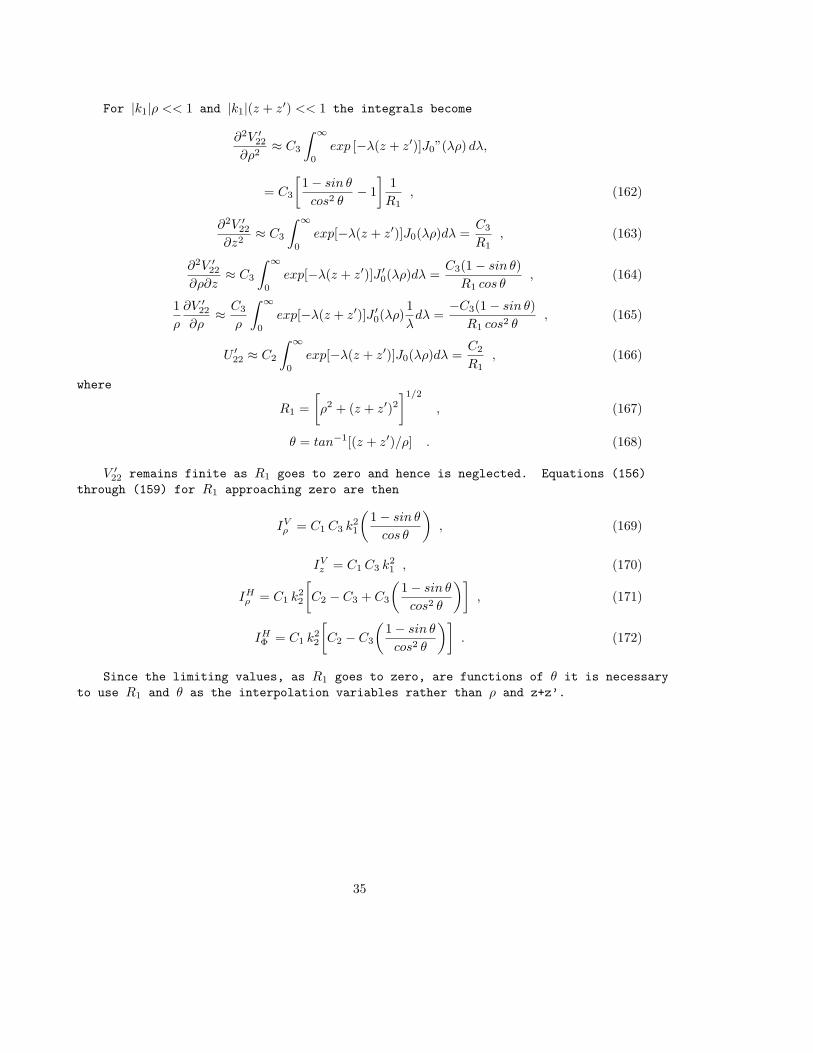
For |k1|ρ << 1 and |k1|(z + z′) << 1 the integrals become

∂2V ′22

∂ρ2≈ C3

∫ ∞

0

exp [−λ(z + z′)]J0”(λρ) dλ,

= C3

[

1 − sin θ

cos2 θ− 1

]

1

R1, (162)

∂2V ′22

∂z2≈ C3

∫ ∞

0

exp[−λ(z + z′)]J0(λρ)dλ =C3

R1, (163)

∂2V ′22

∂ρ∂z≈ C3

∫ ∞

0

exp[−λ(z + z′)]J ′

0(λρ)dλ =C3(1 − sin θ)

R1 cos θ, (164)

1

ρ

∂V ′22

∂ρ≈ C3

ρ

∫ ∞

0

exp[−λ(z + z′)]J ′

0(λρ)1

λdλ =

−C3(1 − sin θ)

R1 cos2 θ, (165)

U ′

22 ≈ C2

∫ ∞

0

exp[−λ(z + z′)]J0(λρ)dλ =C2

R1, (166)

where

R1 =

[

ρ2 + (z + z′)2]1/2

, (167)

θ = tan−1[(z + z′)/ρ] . (168)

V ′22 remains finite as R1 goes to zero and hence is neglected. Equations (156)

through (159) for R1 approaching zero are then

IVρ = C1 C3 k2

1

(

1 − sin θ

cos θ

)

, (169)

IVz = C1 C3 k2

1 , (170)

IHρ = C1 k2

2

[

C2 − C3 + C3

(

1 − sin θ

cos2 θ

)]

, (171)

IHΦ = C1 k2

2

[

C2 − C3

(

1 − sin θ

cos2 θ

)]

. (172)

Since the limiting values, as R1 goes to zero, are functions of θ it is necessary

to use R1 and θ as the interpolation variables rather than ρ and z+z’.

35

Figures 7 through 10 are plots of the surfaces to which interpolation is applied

for typical ground parameters. The width of the region of relatively rapid variation

along the R1 axis appears to be proportional to the wavelength in the lower medium

and hence is concentrated closer to R1 = 0 for larger dielectric constants. At a

finite R1, the functions approach zero as ǫ1 and σ1 become large. When loss is small

the strong wave in the lower medium results in a significant evanescent wave along

the interface in the upper medium as shown in figure 11.

36

Figure 7(a). Re(IVρ ) for ǫ1/ǫ0=4, σ1=0.001 mhos/m, frequency = 10 MHz.

Figure 7(b). Im(IVρ ) for ǫ1/ǫ0=4, σ1=0.001 mhos/m, frequency = 10 MHz.

37

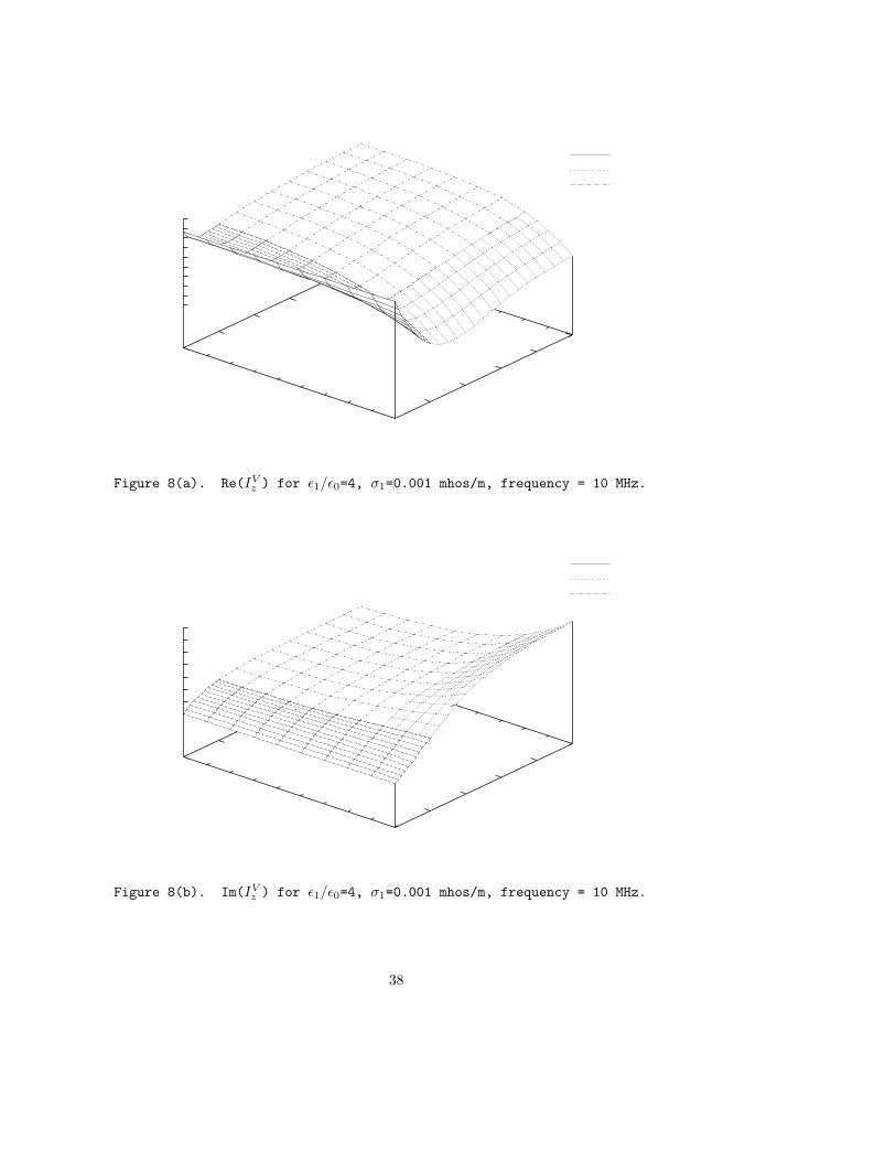
Figure 8(a). Re(IVz ) for ǫ1/ǫ0=4, σ1=0.001 mhos/m, frequency = 10 MHz.

Figure 8(b). Im(IVz ) for ǫ1/ǫ0=4, σ1=0.001 mhos/m, frequency = 10 MHz.

38

Figure 9(a). Re(IHρ ) for ǫ1/ǫ0=4, σ1=0.001 mhos/m, frequency = 10 MHz.

Figure 9(b). Im(IHρ ) for ǫ1/ǫ0=4, σ1=0.001 mhos/m, frequency = 10 MHz.

39

Figure 10(a). Re(IHΦ ) for ǫ1/ǫ0=4, σ1=0.001 mhos/m, frequency = 10 MHz.

Figure 10(b). Im(IHΦ ) for ǫ1/ǫ0=4, σ1=0.001 mhos/m, frequency = 10 MHz.

40

Figure 11(a). Re(IHρ ) for ǫ1/ǫ0=16, σ1=0.000 mhos/m, frequency = 10 MHz.

Figure 11(b). Im(IHρ ) for ǫ1/ǫ0=16, σ1=0.000 mhos/m, frequency = 10 MHz.

41

In NEC the interpolation region from 0 to l wavelength in R1 is divided into three

grids, as shown in figure 12, on which bivariate cubic interpolation is used. For

a given point, the correct grid region is determined and cubic surfaces in R1 and

θ, fit to a 4-point by 4-point region containing the desired point, are evaluated for

each of the four quantities IVρ , IV

z , IHρ , and IH

Φ . The grid point spacings used are:

Grid ∆R1 ∆θl 0.02λ 10o

2 0.05λ 5o

3 0.l0λ 10o

These were determined by numerical tests to keep relative errors of interpolation

generally in the range of 10−3 to 10−4. A smaller ∆R1 could be needed in grid 2 for

large ǫ1 and small σ1 to handle the rapidly oscillating evanescent wave, but this is

easily changed in the code.

The field evaluation in NEC uses variable-interval-width Romberg integration over

the current distribution. At each integrand evaluation, the components IVρ , IV

z , IHρ , and

IHΦ are obtained by interpolation, and the field components are combined according

to the direction of the current. The numerical integral is then combined with the

free-space field and with the image field multiplied by (k21−k2

2)/(k21 +k2

2) to obtain

the total field over ground.

When R1 from the observation point to the center of a wire segment is greater than

one wavelength, the field is evaluated by Norton’s asymptotic approximations (ref.

26) rather than the above method. Norton’s formulas are given in Part II of this manual

under subroutine GWAVE. Although they are less accurate than the Sommerfeld integral

forms and require longer to evaluate than the interpolation, their use permits truncating

the interpolation tables. Another approximation used for R1 greater than a wavelength

is to treat the current distribution on a segment as a lumped current element with

the correct moment rather than integrating over the current distribution.

42

Grid 1

Grid 2

Grid 3

0o

20o

40o

60o

90o

θ

0

b

0.2λ

b

0.4λ

b

0.6λ

b

0.8λ

b

1.0λ

b

Figure 12. Grid for Bivariate Interpolation of I’s.

43

2. NUMERICAL EVALUATION OF THE SOMMERFELD INTEGRALS

The integrals in equations (l48) through (l53) are evaluated by numerical integration

along contours in the complex λ plane. Although these integrals differ from the usual

Sommerfeld integrals in the Dl and D2 terms, they are the same in the properties important

to numerical integration --- the locations of poles and branch cuts and the exponential

behavior of the Bessel and exponential functions. The behavior of the integrands and

numerical methods for evaluating the integrals are discussed in detail by Lytle and

Lager (ref. 27). This section describes the particular method used in NEC, which is

basically the same as in the code WFLLL2A.

Since the integrands of the six integrals are similar, V ′22 will be considered as

typical. The integrands have branch cuts from the ±k1 to infinity and ±k2 to infinity

due to the square roots in γ1 and γ2 respectively. The branch cuts are chosen to be

vertical, as shown in figure 13. The implications of this choice of branch cuts and

the choice of Reimann sheets are discussed in ref. 27.

The key to rapid convergence in the numerical integration is to exploit the exponential

behavior of the exponential and Bessel functions for large λ. The integration contour

is deformed from the real axis into the complex plane avoiding branch cuts and taking

account of poles, to optimize convergence. With the vertical branch cuts chosen, there

are no real poles on the primary Reimann sheet although virtual poles from D1 or D2

result in a near singularity in the region of ±k2 when k1 approaches k2 (free-space

limit). Hence the integration contour should avoid the real axis in this region.

λR

λI

p + jpb

b

k2

b

k1

b

−k2

b

−k1

Figure 13. Contour for Evaluation of Bessel Function Form of Sommerfeld Integrals.

The contour used with the form of the integrals in equations (l48) through (l53)

is shown in figure 13. The dominant factor for convergence in this case is the exponential

function as λR increases. The Bessel function oscillates with slow convergence for

increasing λR and grows exponentially as |λI | increases. Hence it is of little help

in convergence but restricts the contour to small ρ|λI |. The break in the contour is

at λ = p + jp where p is the minimum of 1/ρ and 1/(z + z′).

Integration along this contour becomes difficult when (z + z′)/ρ is small since

there may be many oscillations of the Bessel function before convergence. In this

44

case an alternate form of the integrals is used which for V ′22 is

V ′

22 =1

2

∫ +∞

−∞

D2 exp

[

− γ2(z + z′)

]

H(2)0 (λρ)λdλ, (173)

Since the Hankel function of type 2 decays exponentially as λI becomes negative it

provides rapid convergence without the exp − γ2(z + z′) factor. The behavior of the

integrand can be seen from the large argument approximation

exp

[

− γ2(z + z′)

]

H(2)0 (λρ) ≈

√

2j

πλρ

exp − λ[±(z + z′) + jρ]

,

where, for the vertical branch cuts, the ± sign is

+ for λR > −k2 and λI > 0 ,

+ for λR > k2 and λI < 0 ,

− otherwise.

Thus, an integration path having

λI < 0

and

λI/λR = −ρ/(z + z′) for λR > k2

or

λI/λR = ρ/(z + z′) for λR < k2

results in exponential convergence with little oscillation. The basic contour used

with the Hankel function form is shown in figure 14 where

a = −j 0.4 k2 ,

b = (0.6 + j 0.2) k2 ,

c = (1.02 + j 0.2) k2 ,

d = 1.01 k1R+ j 0.99 k1I

,

θ = tan−1(ρ

z + z′) .

45

λR

λI

b

k2

bk1

b

−k2

b

−k1

ba

bb

b

c

bd

Figure 14. Contour for Evaluation of Hankel Function Form of Sommerfeld Integrals.

To avoid the near singularity as k1 approaches k2, the real part of d is not allowed

to be less than 1.1 k2. This contour provides rapid convergence except when z+z′ is

small, |k1ρ| is large, and k1I/k1R

is small. There may then be many oscillations between

c and d with little convergence. In such a case the contour in figure l5 is used where

e = k1 + (−0.1 + 0.2j) ,

f = k1 + (0.1 + 0.2j) .

λR

λI

b

k2

b

b

−k2

b

−k1

ba

bb

b

c

bbe

bf

Figure 15. Contour for Evaluation of Hankel Function Form of Sommerfeld Integrals when Real Part k1 is Large and

Imaginary k1 is Small.

The Hankel function form of the integrals provides rapid convergence for small

z + z′ including the case of z = z′ = 0. For small ρ, however, the pole at λρ = 0requires special treatment. In NEC the Hankel function form with the contour of figure

14 or l5 is used when ρ is greater than (z+z′)/2 and the Bessel function form is used

otherwise.

46

Integration along the contours is accomplished by adaptive interval-width Romberg

integration. On the sections going to infinity, adaptive Romberg integration is applied

to successive subsections of length p, where p is the minimum of 0.2π/ρ or 0.2π/(z+z′), and Shanks’ nonlinear transformation (ref. 28) is applied to the sequence of partial

sums to accelerate convergence. When ρ and z + z′ are both small, the integration

interval, p, may be large since the exponential and Bessel functions change slowly

and the remaining factors are easily integrated once λ becomes large. For the Bessel

function form of the integrals the minimum for R1 = [ρ2+(z+z′)2]1/2 is limited only

by the maximum number size for the computer. For the Hankel function form the minimum

R1 is about 10−5 wavelengths due to the pole at λρ = 0. Either ρ or z + z′ may be

zero.

The numerical integration results for small R1 were checked against results from

a series approximation (ref. 25) and were in very close agreement. For larger values

of R1 the results from different integration contours were compared as a validation

test. Results for the modified Sommerfeld integrals were also checked with normal

integrals used in the code WFLLL2A. Earlier studies for the code WFLLL2A, which is

capable of computing the field across the interface, verified the continuity of the

computed tangential E field across the interface (ref. 44).

The average time required to evaluate the integrals for a given p and z+z’ on a

CDC 7600 computer is about 0.06 s. Thus about l5 s are required to fill the interpolation

grid. Once the grid has been computed and stored, the time to fill an interaction

matrix, using interpolation and the Norton formulas, is about four times that for free

space.

3. THE IMAGE AND REFLECTION-COEFFICIENT METHODS

The use of a reflected image is a simple and fast way to model the effect of a

ground plane. If the ground is perfectly conducting, the structure and its image are

exactly equivalent to the structure over the ground. Since use of the image only doubles

the time to compute the field, it is always used with a perfect ground. NEC also includes

an image approximation for a finitely conducting ground in which the image fields are

modified by the Fresnel plane-wave reflection coefficients. Although this is far from

exact for a finite ground, it has been shown to provide useful results for structures

that are near too. near to the ground (refs. 21 and 22). When it can be used, the

reflection coefficient method is about twice as fast as the Sommerfeld/Norton method

and avoids the need of computing the interpolation grid.

Implementation of the image and reflection coefficient methods in the code is very

simple. The Green’s function for a perfectly conducting ground is the sum of the free-space

Green’s function of the source current element and the negative of the free-space Green’s

function of the image of the source reflected in the ground plane. For the electric

field, with free-space Green’s dyad ¯G(~r, ~r′) defined in equation (1), Green’s dyad for

47

a perfect ground is¯Gpg(~r, ~r

′) = ¯G(~r, ~r ′) + ¯GI(~r, ~r′) , (174)

where¯GI(~r, ~r

′) = −¯Ir · ¯G(~r, ¯Ir · ~r ′) , (175)

¯Ir = xx + yy + zz .

¯Ir is a dyad that produces a reflection in the z = 0 plane when used in a dot product.

For the magnetic field with free-space Green’s dyad

¯Γ(~r, ~r ′) = ¯I ×∇ ′ g(~r, ~r ′) (176)

the Green’s dyad over a perfect ground is

¯Γpg = ¯Γ(~r, ~r ′) + ¯ΓI(~r, ~r′) (177)

¯ΓI(~r, ~r′) = −¯Ir · ¯Γ(~r, ¯Ir · ~r ′) (178)

The reflection coefficient method for finitely conducting ground uses the image

fields modified by the Fresnel reflection coefficients. The Fresnel reflection coefficients,

which are strictly correct only for an infinite plan-wave field, depend on the polarization

or the incident field with respect to the plane of incidence (i.e., the plane containing

the normal to the ground and the vector in the direction of propagation of the wave).

The two cases are illustrated in figure l6 where the wave with E in the plane of incidence

is termed vertically polarized and E normal to the plane of incidence as horizontally

polarized. The Fresnel reflection coefficient for vertically polarized waves is

RV =cos θ − ZR

√

1 − Z2R sin2 θ

cos θ + ZR

√

1 − Z2R sin2 θ

(179)

where

cos θ = −k · z ,

ZR =

(

ǫ1ǫ0

− jσ1

ωǫ0

)−1/2

.

The reflected fields are then

~EVR = −RV (¯IR · ~EV ) ,

~HVR = RV

~HV .

48

b

k

b

kR

~HV

~HVR

~EV

~EVR

ǫ0 , µ0

ǫ1 , µ0 , σ1

θθ

(a) Reflection of Vertically Polarized Wave

b

k

b

kR

~Eh

~EhR

~Hh

~HhR

ǫ0 , µ0

ǫ1 , µ0 , σ1

θθ

(b) Reflection of Horizontally Polarized Wave

Figure 16. Plane-Wave Reflection at an Interface

49

For horizontally polarized waves, the reflection coefficient is

RH =

−(

ZR cos θ −√

1 − Z2R sin2 θ

)

ZR cos θ +√

1 − Z2R sin2 θ

, (180)

and~Eh

R = −RH~Eh ,

~HhR = RH

(

¯IR · ~Hh

)

.

An arbitrarily polarized incident plane wave must be resolved into horizontal and vertical

components to determine the reflected field. Thus, if p is the unit vector normal

to the plane of incidence, the reflected field due to an incident field ~E is

~ER = RH( ~EI · p)p + RV

[

~EI − ( ~EI · p)p

]

= RV~EI + (RH − RV )( ~EI · p)p , (181)

where ~EI is the incident field reflected in a perfectly conducting ground, or the fie1d

due to the image of the source. Use of the image field in equation (181) accounts

for the changes in sign and vector direction of the incident field that were shown

explicitly for the vertically and horizontally polarized cases. For the magnetic field,

~HR = RH~HI + (RV − RH)( ~HI · p)p , (182)

with ~HI the field of the image of the source.

Applying the Fresnel reflection coefficients to the near fields, the electric field

at ~r due to the image of a current element at ~r ′ can be written

¯GR(~r, ~r ′) = RV¯GI(~r, ~r

′) + (RH − RV )

[

¯GI(~r, ~r′) · p

]

p , (183)

where

p = ~p/|~p| ,

~p = (~r − ~r ′) × z ,

and ¯GI is the Green’s function for the image of the source in a perfect ground as defined

in equation (l75). For magnetic field, the Green’s dyad for the modified image is

¯ΓR(~r, ~r ′) = RH¯ΓI(~r, ~r

′) + (RV − RH)

[

¯ΓI(~r, ~r′) · p

]

p . (184)

The Green’s functions for electric and magnetic fields, over an imperfectly conducting

ground, resulting from the reflection coefficient approximation are then

¯Gg(~r, ~r′) = ¯G(~r, ~r ′) + ¯GR(~r, ~r ′) , (185)

¯Γg(~r, ~r′) = ¯Γ(~r, ~r ′) + ¯ΓR(~r, ~r ′) . (186)

50

Use of the Green’s function’s ¯Gg and ¯Γg results in a straightforward extension

of the EFIE and MFIE for structures over an imperfect ground.

NEC also includes a reflection coefficient approximation for a radial wire ground

screen, as used by Miller and Deadrick (ref. 29). This is based on an approximation

developed by Wait (ref. 30) for the surface impedance of the radial-wire ground screen

on an imperfectly conducting ground, as the parallel combination of the surface impedance,

ζ1, of the ground plane

ζ1 =

(

jµ0ω

σ1 + jǫ1ω

)1/2

,

and an approximate surface impedance Zg of the ground screen

Zg(ρ) =jµ0ωρ

Nln

(

ρ

NC0

)

.

The ground screen impedance assumes a parallel wire grid having the wire spacing that

the radial wires have at a distance ρ from the center. N is the number of radial wires

in the screen, and C0 is the radius of the wires. The surface impedance of the ground

screen on an imperfect ground is then

ζe =ζ1Zg

ζ1 + Zg.

From the definition of surface impedance,

Etangential = ζeHtangential

at the surface. Using the fact that E and H in the incident wave are related by ηthe free-space impedance, reflection coefficients are derived as

RH =η − ζe cos θ

η + ζe cos θ,

and

RV =η cos θ − ζe

η cos θ + ζe.

This is the form the Fresnel reflection coefficients take when the index of refraction

is large compared to unity (|ZR|2 << 1). This condition is satisfied in most realistic

problems; furthermore the surface-impedance boundary condition is a valid approximation

only when the refractive index of the ground is large compared to unity. The surface

impedance is used in conjunction with the reflection coefficient method previously

discussed to provide an approximate model of a radial-wire ground screen.

Due to the assumption of specular reflection, only the properties of the ground

directly under a vertical antenna will affect its current distribution. At the origin

of the radial-wire ground screen, the impedance is zero (Zg is not allowed to be negative)

so the impedance and current distribution of a vertical antenna at the origin will

be the same as over a perfect conductor. The far fields, however, will demonstrate

the effect of the screen as the specular point moves away from the origin. For antennas

other than the vertical antenna, it should be pointed out that the inherent polarization

51

sensitivity of the screen (i.e., E parallel or perpendicular to the ground wires) has

not been considered in this approximation. When limited accuracy can be accepted this

ground screen approximation provides a large time saving over explicit modeling with

the Sommerfeld/Norton method since the ground screen does not increase the number of

unknowns in the matrix equation.

52

Section V - Modeling of AntennasPrevious sections have dealt with the problem of determining the current induced

on a structure by an arbitrary excitation. We now consider some specific problems

in modeling antennas and scatterers; including models for a voltage source on a wire,

lumped and distributed loads, nonradiating networks, and transmission lines. Calculations

of some observable quantities are also covered including input impedance, radiated

field, and antenna gain.

l. SOURCE MODELING

The approach used in NEC is applicable to a number of electromagnetic analysis

problems. For receiving antennas and EMP studies, the excitation is the field of an

incident plane wave and the desired response is the induced current at one or more

points on the structure. In scattering analysis the excitation is still an incident

plane wave, but the desired response is the field radiated by the induced currents.

In the case of a wire transmitting antenna, however, the excitation is generally a

voltage source on the wire. The antenna source problem has received a considerable

amount of attention in the literature. A rather thorough exposition on the appropriate

source configuration for the linear dipole antenna has been given by King (ref. 3l).

The delta-function source, which may be visualized as an infinitesimally thin, circumferential

belt of axially directed electric field [or, alternatively, as a frill of magnetic

current at the antenna feed point (ref. 32)], is convenient mathematically, but of

somewhat questionable physical realizability. Since the excitation can be specified

only at discrete points in NEC, a delta-function source is not feasible.

A useful source model, however, is an electric field specified at a single match

point. For a voltage source of strength V on segment i, the element in the excitation

vector corresponding to the applied electric field at the center of segment i is set

to

Ei =V

∆i, (187)

where ∆i is the length or segment i. The direction of E1 is toward the positive end

of the voltage source so that it pushes charge in the same direction as the source.

The field at other match points is set to zero. The actual effective voltage is the

line integral of the applied field along the wire. This cannot be determined beforehand

since the field is known only at segment centers, but can be determined after the solution

or current by integrating the scattered field produced by the current. For equal length

segments in the vicinity of the source this field, which must be the negative of the

applied field at every point on the wire, is nearly constant over segment i and drops

sharply at the segment ends. This results in an actual voltage of approximately ∆iEi

as assumed in equation (187). When the source segment and adjacent segments are not

of equal length, however, the actual voltage, obtained by integrating the scattered

field, may differ from the intended value.

Ideally, this source model applies a voltage V between the ends of the source segment.

Hence, the antenna input admittance could be computed as the current at the segment

ends or, in an unsymmetric case, the average of the current at the two ends, divided

53

by the applied voltage. In practice the segment is sufficiently short so that the

current variation over its length is small and the current at the center can be used

rather than the ends. When segment lengths in the source region are unequal, the computed

input admittance may be inaccurate due to the discrepancy between the actual and assumed

voltages. Use of the actual voltage, obtained by integrating the near field, will

generally give an accurate admittance although it will require additional effort for

computation.

An alternate source model that is less sensitive to the equality of segment lengths

in the source region is based on a discontinuity in the derivative of current. This

source model is similar to one used by Andreasen and Harris (ref. 33), and its use

in a program similar to NEC was reported by Adams, Poggio, and Miller (ref. 24). For

this model, the source region is viewed as a biconical transmission line with feed

point at the source location as illustrated in figure 17. The voltage between a point

at s and the symmetric point on the other side of the line is then related to the derivative

of the current by the transmission line equation,

V (s) = − jZ0∂I(ks)

∂(ks), (188)

where Z0 is the characteristic impedance of the transmission line. The characteristic

impedance of a biconical transmission line of half-angle θ is

54

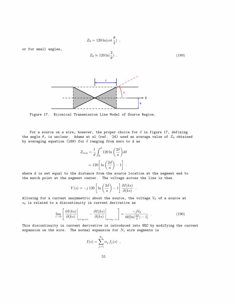
Z0 = 120 ln(cotθ

2) ,

or for small angles,

Z0 ≈ 120 ln(2

θ) . (189)

S

a

θ

δ

Figure 17. Biconical Transmission Line Model of Source Region.

For a source on a wire, however, the proper choice for δ in figure 17, defining

the angle θ, is unclear. Adams at al (ref. 24) used an average value of Z0 obtained

by averaging equation (l89) for δ ranging from zero to d as

Zavg =1

d

∫ d

0

120 ln

(

2δ

a

)

dδ

= 120

[

ln

(

2d

a

)

− 1

]

.

where d is set equal to the distance from the source location at the segment end to

the match point at the segment center. The voltage across the line is then

V (s) = −j 120

[

ln

(

2d

a

)

− 1

]

∂I(ks)

∂(ks).

Allowing for a current unsymmetric about the source, the voltage V0 of a source at

s0 is related to a discontinuity in current derivative as

limǫ→0

[

∂I(ks)

∂(ks)

∣

∣

∣

∣

∣

s=s0+ǫ

− ∂I(ks)

∂(ks)

∣

∣

∣

∣

∣

s=s0−ǫ

]

=−jV0

60[ln(2da ) − 1]

. (190)

This discontinuity in current derivative is introduced into NEC by modifying the current

expansion on the wire. The normal expansion for Ns wire segments is

I(s) =

Ns∑

j=1

αj fj(s) ,

55

where the basis functions, fj, are defined in section III-l such that I(s) has continuous

value and derivative along wires, and satisfies Kirchoff’s law and a condition on charge

density at junctions.

For a current-slope-discontinuity source at the first end of segment l, the current

expansion is modified to

I(s) =

Ns∑

j=1

αj fj(s) + βlf∗

l (s) , (191)

where f∗

l is a basis function for segment l, as defined in section III-1, but computed

as if the first end of segment l were a free end and the segment radius were zero.

Hence, f∗

l goes to zero with nonzero derivative at the source location.

If f∗

l on segment l is

f∗

l = A∗

l + B∗

l sin k(s − sl) + C∗

l cos k(s − sl)

|s − sl| < ∆l/2 ,

then∂

∂(ks)f∗

l (s)

∣

∣

∣

∣

s=sl−∆l/2

= B∗

l cos(k∆l/2) + C∗

l sin(k∆l/2) .

Since the sum of the normal basis functions has continuous value and derivative

at s = sl−∆l/2, the current in equation (191) has a discontinuity in derivative of

limǫ→0

∂

∂(ks)I(s)

∣

∣

∣

∣

s=sl−∆l/2+ǫ

− ∂

∂(ks)I(s)

∣

∣

∣

∣

s=sl−∆l/2−ǫ

= βl

B∗

l cos(k∆l/2) + C∗

l sin(k∆l/2)

.

Hence, from equation (190), a source voltage of V0 requires a value of βl in the current

expansion of

βl =−j V0

60

[

ln

(

∆l

al

)

− 1

][

B∗

l cos(k∆l/2) + C∗

l sin(k∆l/2)

]−1

. (192)

The linear system for the current expansion constants, obtained by substituting

equation (19l) for f in equation (l8), is

Ns∑

j=1

αj < wi, Lfj >=< wi, e > −βl < wi, f∗

l > i = 1, ..., Ns (193)

In matrix notation, corresponding to equation (l9),

[G] [A] = [E] + βl [F ] . (194)

where Fi is the excitation or segment or patch equation number i due to the field of

f∗

l , and Ei is the excitation for segment or patch equation number i from other sources

56

(if there are any). The interaction matrix G is independent of this source as it is

of other sources. The solution for the expansion coefficients is then

[A] = [G−1] [E] + βl [F ] ,

where Fi supplies the coefficients αj in equation (l9l) to determine the current. This

method is easily extended to several sources. The modified basis function f∗

l appears

to introduce an asymmetry into the current, but this is not the case since the other

basis function amplitudes are free to adjust accordingly.

The current-slope-discontinuity source results in an effective applied field that

is much more localized in the source region than that of the constant-field source

defined by equation (187). The difference is shown in near-field plots for the two

source models in figure 18, taken from Adams et al (ref. 24). The near fields are

for a half wavelength dipole antenna with Ω = 15 [Ω = 2 ln(L/a), L = length, a = radius]

and with 10 segments on half of the antenna covered by the plots. The constant-field

source is seen to result in a nearly rectangular field distribution in the source region

while the field of the slope-discontinuity source approaches a delta function. The

integrals of these two source-field distributions yield approximately the same voltages

however.

With the slope-discontinuity-source model, the input admittance is the ratio of

the current at the segment end, where the source is located, to the source voltage.

Adams et al also present results showing the effect on admittance of varying the source-segment

length relative to the lengths of adjacent segments, showing that the slope-discontinuity

source is much less sensitive to segment length than is the constant-field source.

The two segments on opposite sides of the source must have equal lengths and radii

however. For very short segment lengths, the slope-discontinuity model may break down

although, as with the constant-field source, the correct admittance can be obtained

by integrating the near field to obtain the source voltage.

57

Figure 18. Field Plot for a Linear Dipole. Ω=15.

58

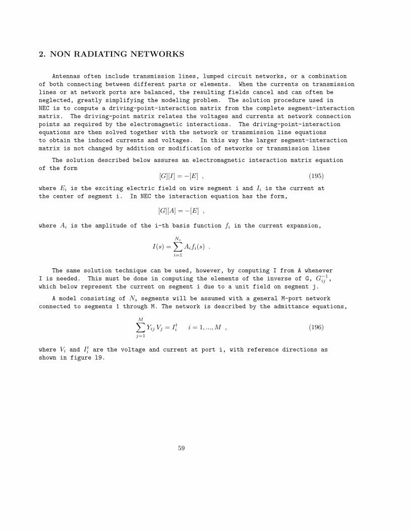
2. NON RADIATING NETWORKS

Antennas often include transmission lines, lumped circuit networks, or a combination

of both connecting between different parts or elements. When the currents on transmission

lines or at network ports are balanced, the resulting fields cancel and can often be

neglected, greatly simplifying the modeling problem. The solution procedure used in

NEC is to compute a driving-point-interaction matrix from the complete segment-interaction

matrix. The driving-point matrix relates the voltages and currents at network connection

points as required by the electromagnetic interactions. The driving-point-interaction

equations are then solved together with the network or transmission line equations

to obtain the induced currents and voltages. In this way the larger segment-interaction

matrix is not changed by addition or modification of networks or transmission lines

The solution described below assures an electromagnetic interaction matrix equation

of the form

[G][I] = −[E] , (195)

where Ei is the exciting electric field on wire segment i and Ii is the current at

the center of segment i. In NEC the interaction equation has the form,

[G][A] = −[E] ,

where Ai is the amplitude of the i-th basis function fi in the current expansion,

I(s) =

Ns∑

i=1

Aifi(s) .

The same solution technique can be used, however, by computing I from A whenever

I is needed. This must be done in computing the elements of the inverse of G, G−1ij ,

which below represent the current on segment i due to a unit field on segment j.

A model consisting of Ns segments will be assumed with a general M-port network

connected to segments 1 through M. The network is described by the admittance equations,

M∑

j=1

Yij Vj = Iti i = 1, ...,M , (196)

where Vi and Iti are the voltage and current at port i, with reference directions as

shown in figure l9.

59

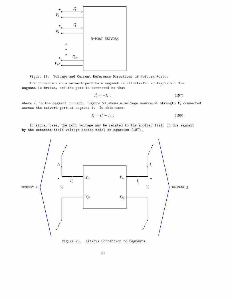
M-PORT NETWORK

b+

bV1

b+

bV2

b

b

b

b+

bVM

It1

It1

ItM

Figure 19. Voltage and Current Reference Directions at Network Ports.

The connection of a network port to a segment is illustrated in figure 2O. The

segment is broken, and the port is connected so that

Iti = −Ii , (197)

where Ii is the segment current. Figure 21 shows a voltage source of strength Vi connected

across the network port at segment i. In this case,

Iti = Ig

i − Ii . (198)

In either case, the port voltage may be related to the applied field on the segment

by the constant-field voltage source model or equation (187).

Yij

YjjYji

YiiIt1

Itj

+ +

Vi Vj

Ii Ij

SEGMENT i SEGMENT j

Figure 20. Network Connection to Segments.

60

Yij

YjjYji

YiiIt1

Itj

+ +

Vi Vj

Ii Ij

SEGMENT i SEGMENT jIgi

Figure 21. Network Port and Voltage Source Connected to a Segment.

We will assume that segments l through M1 are connected to network ports without

voltage sources, and segments M1+1 through M are connected to network ports with

voltage sources. The remaining segments have no network connections but may have voltage

sources. In addition all of the segments may be excited by an incident field represented

by EIi on segment i. The total field on segment i is then

Ei =Vi

∆i+ EI

i .

where Vi is a gap voltage, due either to a network port or voltage source, and ∆i is

the segment length.

Equation (195) may be solved for current as

Ii = −Ns∑

j=1

G−1ij Ej i = 1, ..., Ns , (199)

Where G−1ij is the (i,j)-th element of the inverse of matrix, G. Before evaluating

equation (199), however, the unknown port voltages, Vi, for i = l, ...,M1 must be determined.

Hence, equation (l99) is written with all known quantities on the right-hand side as

61

M1∑

j−1

G−1ij EP

j + Ii = Bi i = 1, ...,M1 , (200)

where

EPj =

Vj

∆j.

and

Bi = −M1∑

j=1

G−1ij EI

j −Ns∑

M1+1

G−1ij Ej .

Similarly, the network equations (196) are written using equation (197) as

M1∑

j−1

Y ′

ijEPj + Ii = Ci i = 1, ...,M1 , (201)

where

Y ′

ij = ∆jYij ,

Ci = −M∑

j=M1+1

YijVj .

The current is then eliminated between equations (200) and (201) to yield

M1∑

j=1

(

G−1ij − Y ′

ij

)

EPj = Bi − Ci i = 1, ...,M1 . (202)

The solution procedure is then to solve equation (202) for EPj for j = 1, ...,M1.

Then, with the complete excitation vector determined, use equation (l99) to determine

Ii for i = l, ..., Ns. Finally, the remaining network equations with equation (198) are

used to compute the generator currents as

Igi =

M∑

j−1

YijVj + Ii i = M1 + 1, ...,M . (203)

The currents Igi determine the input admittances seen by the sources. In NEC the

general M-port network used here is restricted to multiple two-port networks, each

connecting a pair of segments.

62

3. TRANSMISSION LINE MODELING

Transmission lines interconnecting parts of an antenna may be modeled either explicitly

by including the transmission 1ine wires in the thin-wire model, or implicitly by the

method described in the preceding section for nonradiating networks. For an implicit

model, the short-circuit-admittance parameters of the transmission line viewed as a

two-port network are

Y11 = Y22 = −jY0 cot(kl) ,

Y12 = Y21 = jY0 csc(kl) ,

where Y0 is the characteristic admittance of the line, k is the wave number (2π/λ),and l is the length of the 1ine. If a separate admittance element is connected across

the end of a transmission 1ine, its admittance is added to the self-admittance of that

network port.

The implicit model is limited, however, in that it neglects interaction between

the transmission line and the antenna and its environment. This approximation is justified

if the currents in the line are balanced, i.e., in a log periodic dipole antenna, and

in general if the transmission line lies in an electric symmetry plane. The balance

can be upset, however if the transmission line is connected to an unbalanced load or

by unsymmetric interactions. If the unbalance is significant, the transmission line

can modeled explicitly by including the wires in the thin-wire model. The explicit

model is completely general, and yields accurate results since the sine, cosine, and

constant current expansion in NEC is a good representation of the sinusoidal transmission

line currents. The accuracy is demonstrated in figure 22 for transmission lines terminated

in short circuit, open circuit, and matched loads.

The explicit transmission line model is, of course, less efficient in computer

time and storage because of the additional segments required. In cases where the physical

line presence does have a significant effect on the results, the effect may be modeled

by explicitly modeling a single conductor of the line while using the implicit model

to represent the balanced current component.

63

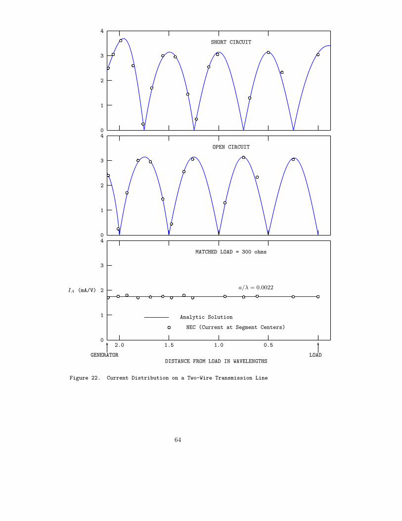
SHORT CIRCUIT

0

1

2

3

4

OPEN CIRCUIT

0

1

2

3

4

a/λ = 0.0022

MATCHED LOAD = 300 ohms

0

1

2

3

4

Analytic Solution

NEC (Current at Segment Centers)

GENERATOR LOADDISTANCE FROM LOAD IN WAVELENGTHS

2.0 1.5 1.0 0.5

IA (mA/V)

Figure 22. Current Distribution on a Two-Wire Transmission Line

64

4. LUMPED OR DISTRIBUTED LOADING

Thus far, we have assumed that all structures to be modeled are perfect electric

conductors. The EFIE is easily extended to imperfect conductors by modifying the boundary

condition from equation (4) to

n(~r) ×[

~ES(~r) + ~EI(~r)]

= Zs(~r)

[

n(~r) × ~Js(~r)

]

,

where Zs(~r)i is the surface impedance at ~r on the conducting surface. For a wire, the

boundary condition is

s ·[

~Es(~r) + ~EI(~r)

]

= Zw(s)I(s) ,

with ~r and s the position vector and tangent vector at s on the wire and Zw(s) the

impedance per-unit-length at s. The matrix equation can then be written

Ns∑

j=1

Gijαj = −Ei +Zi

∆iIi i = 1, ..., Ns , (204)

where

αj = amplitude of basis function j,

Ei = the incident field on segment i,

I1 = current at the center of segment i,

Zi = total impedance of segment i,

∆i = length of segment i.

The impedance term can be viewed as a constant field model of a voltage source,

as described in section 1, where the voltage is proportional to current. It is assumed

that the current is essentially constant, with value Ii, over the length of the segment,

which is a reasonable assumption for the electrically short segments used in the integral

equation solution.

The impedance term can be combined with the matrix by expressing Ii in terms of

the αj as

Ii =

Ns∑

j−1

αj (Aij + Ci

j) ,

where Aij and Ci

j are the coefficients of the constant and cosine terms, respectively,

in the section of basis function j extending onto segment i. If basis function j does

not extend onto segment i, then Aij and Ci

j are zero. The matrix equation modified

by loading is thenNs∑

j=1

G′

ijαj = −Ei i = 1, ..., Ns , (205)

where

G′

ij = Gij −Zi

∆i

(

Aij + Ci

j

)

. (206)

65

For a lumped circuit element, Zi is computed from the circuit equations. For a distributed

impedance, Zi represents the impedance of a length ∆i of wire, which in the case of

a round wire of finite conductivity is given by

Zi =j∆i

ai

√

ωµ

2πσ

[

Ber(q) + jBei(q)

Ber′(q) + jBei′(q)

]

,

where

q = (ωµσ)1/2ai ,

ai = wire radius,

σ = wire conductivity,

Ber = Kelvin function,

Bei = Kelvin function.

This expression takes account of the limited penetration of the field into an imperfect

conductor.

66

5. RADIATED FIELD CALCULATION

The radiated field of an antenna or reradiated field of a scatterer can be computed

from the induced current by using a simplified form of equation (1) valid far from

the current distribution. The far-field

approximation valid when the distance from the current distribution to the observation

point is large compared to both the wavelength and the dimensions of the current distribution,

treats the distance |~r−~r ′| as constant integral except in the phase term, exp(−jk|~r−~r ′|). For a structure consisting of a wire portion with contour L and current distribution~I(s), and a surface portion S with current ~Js(~r), the far-zone field is

~E(~r0) =jkη

4π

exp(−jkr0)

r0×

∫

L

[(

k · ~I(s)

)

k − ~I(s)

]

exp(j~k · ~r)ds

+

∫

S

[

(

k · ~Js(~r

)

k − ~Js(~r)

]

exp(j~k · ~r)dA

, (207)

where ~r0 is the position of the observation point k = ~r0/|~r0|, k = 2π/λ,and ~k = kk.The first integral can be evaluated in closed form over each straight wire segment

for the constant, sine, and cosine components of the basis functions, and reduces to

a summation over the wire segments. With the surface current on each patch represented

by a delta function at the patch center, the second integral becomes a summation over

the patches.

The radiation pattern of an antenna can be computed by exciting the antenna with

a voltage source and using equation (207) to compute the radiated field for a set of

directions in space. Alternatively, since the transmitting and receiving patterns

are required by reciprocity to be the same, the pattern can be determined by exciting

the antenna with plane-waves incident from the same directions and computing the currents

at the source point. The solution procedure in NEC does not guarantee reciprocity,

however, since the different expansion and weighting functions may produce asymmetry

in the matrix. Large differences between the receiving and transmitting patterns of

a significant lack of reciprocity in bistatic scattering are indications of inaccuracy

in the solution, possibly from too coarse a segmentation of the wires or surfaces.

The power gain of an antenna in the direction specified by the spherical coordinates

(θ,Φ) is defined as

GP (θ,Φ) = 4πP (θ,Φ)

Pin,

where P (θ,Φ) is the power radiated per unit solid angle in the direction (θ,Φ), and

Pin is the total power accepted by the antenna from the source. Pin is computed from

the voltage and current at the source as

Pin =1

2Re(V I∗) ,

and

P (θ,Φ) =1

2R2Re( ~E × ~H∗) =

R2

2η( ~E · ~E∗) .

67

is obtained from equation (207) with ~r0 in the direction (θ,Φ) and r0 = R. Directive

gain is similarly defined as

Gd(θ,Φ) = 4πP (θ,Φ)

Prad,

where Prad is the total power radiated by the antenna,

Prad = Pin − Ploss ,

and Ploss is the tota1 ohmic loss in the antenna.

The radiated field of an antenna over ground is modified by the ground interaction,

as discussed in section IV. When the range from the antenna to the observer, R, approaches

infinity, the Sommerfeld formulation for the field reduces exactly to a direct field

determined by equation (207) and a field from the image modified by the Fresnel reflection

coefficient. In some cases, however, when the observer is at a finite distance from

the antenna, the field components proportional to l/R2 may be significant. While the

1/R terms are generally much larger than the l/R2 terms at practical observation distances

from an antenna, the l/R terms vanish at grazing angles over an imperfect ground plane

leaving only the 1/R2 terms, dominated by a term known as the ground wave. The ground

wave is, of course, included in Sommerfeld’s expressions. Norton’s asymptotic approximations

(ref. 26) are used, however since they are more easily evaluated and give adequate

accuracy. Norton’s formulas, which are in Part II of this manua1 under subroutine

GWAVE, are valid for R greater than a few wavelengths and to second order in k21/k2

2.

When the ground wave is included, the field has radial as well as transverse components.

68

6. ANTENNA COUPLING

Coupling between antennas is often a parameter of interest, especially when a receiving

system must be protected from a nearby transmitter. Maximum power transfer between

antennas occurs when the source impedance and receiver load impedance are conjugate-matched

to their antennas. Determination of this condition is complicated by the antenna interaction,

however, since the input impedance of one antenna depends on the load connected to

the other antenna. NEC-2 includes an algorithm for determining the matched loads and

maximum coupling by a method that was added to special versions of the previous codes

NEC-l and AMP (ref. 34).

The coupling problem can be solved in closed form by the Linville method (ref.

35), a technique used in rf amplifier design. The first step is to determine the two-port

admittance parameters for the coupled antennas by exciting each antenna with the other

short-circuited and computing the self and mutual admittances from the currents computed

by NEC. The maximum coupling is then

GMAX =1

L

[

1 − (1 − L2)1/2

]

,

where

L =|Y12Y21|

2Re(Y11)Re(Y22) − Re(Y12Y21).

The matched load admittance on antenna 2 for maximum coupling is

YL =

[

1 − ρ

1 + ρ+ 1

]

Re(Y22) − Y22 ,

where

ρ =GMAX(Y12Y21)

∗

|Y12Y21|,

and the corresponding input admittance of antenna 1 is

YIN = Y11 −Y21Y12

YL + Y22.

69

References

1. Miller, E. K. et al, Final Technical Report of the Log-Periodic Scattering Ar-ray Program, MBAssociates Report No. MB-R-70/l05, Contract No. F04J0l-68-C-0188,

l970.

2. RCS Computer Program BRACT, Log-Periodic Scattering Array Program - II, MBAssociates

Report No. MB-R-69/46, Contract No. F0470l-68-C-0188, 1969.

3. Antenna Modeling Program - Composite User’s Manual, MBAssociates Report

No. MB-R-74/46, 1974.

4. Antenna Modeling Program - Engineering Manual, MBAssociates Report No. MB-R-74/62,

l974.

5. Antenna Modeling Program - Systems Manual, MBAssociates Report No. MB-R-74/62,

l974.

6. Antenna Modeling Program - Supplementary Computer Program Manual (AMP2),MBAssociates Report No. MB-R-74/62, l975.

7. Numerical Electromagnetic Code (NEC-1) Part III: NEC User’s Guide, Lawrence

Livermore Laboratory, 1977.

8. Numerical Electromagnetic Code (NEC-1) Part II: NEC Program Description -Code, Lawrence Livermore Laboratory, 1977.

9. Albertsen, N. C., Hansen, J. E., and Jensen, N. E., Computation of SpacecraftAntenna Radiation Patterns, The Technical University of Denmark, Lyngby, Denmark,

June 1972

10. Poggio, A. J. and Miller, E. K., Integral Equation Solutions of Three Dimen-sional Scattering Problems, Chapt. IV in Computer Techniques for Electromag-netics, edited by R. Mittra, Pergamon Press, New York, l973.

11. Poggio, A. J. and Adams, R. W., Approximations for Terms Related to the Ker-nel in Thin-wire Integral Equations, UCRL-51985, Lawrence Livermore Laboratory,

CA, December l9, l975.

12. Van Bladel, J., Electromagnetic Fields, McGraw-Hill, New York, 1964.

13. Harrington, R. F., Field Computation by Moment Methods, MacMi11an, New York,

1968.

14. Yeh, Y. S. and Mei, K. K., Theory of Conical Equiangular Spiral Antennas, PartI - Numerical Techniques, IEEE Trans. Ant. and Prop., AP-15, l967, p. 634.

15. Neureufher, A. R. et al, A Comparison of Numerical Methods for Thin WireAntennas, Presented at the 1968 Fall URSI Meeting, Dept. of Electrical Engineering

and Computer Sciences, University of California Berkeley, l968.

70

16. Miller, E. K. et al, An Evaluation of Computer Programs Using Integral Equa-tions for the Electromagnetic Analysis of Thin Wire Structures, UCRL-75566,

Lawrence Livermore Laboratory, CA, March 1974.

17. Wu, T. T. and King, R. W. P., The Tapered Antenna and Its Application to theJunction Problem for Thin Wires, IEEE Trans. Ant. and Prop., AP-24, No. l,

pp. 42-45, January 1976.

18. Poggio, A. J., Integral Representations for Fields Due to Sources on Open Sur-faces with Applications to End Caps, UCRL-51723, Lawrence Livermore Laboratory,

CA, December 16, 1974.

19. Ralston, A., A First Course in Numerical Analysis, McGraw-Hill, New York, l965.

20. Sommerfeld, A., Partial Differential Equations in Physics, Academic Press New York,

l964.

21. Burke, G. J., Miller, E. K., and Poggio, A. J., Dielectric Ground Interactionswith a Log-Periodic Antenna, Final Report, ECOM-0285-F, U.S. Army Electronics

Command, Fort Monmouth, N.J., l972 (contract DAAB07-70-C-0285).

22. Mi1ler, E. K., Poggio, A. J., Burke, G. J., and Selden, E. S., Analysis of WireAntennas in the Presence of a Conducting Half Space: Part I. The Vertical An-tenna in Free Space. Part II. The Horizontal Antenna in Free Space, UCRL-732l7,

Lawrence Livermore Laboratory, CA, 1972. (Also in Canadian J. Phys.)

23. Lager, D. L. and Lytle, R. J., Fortran Subroutines for the Numerical Evalua-tion of Sommerfeld Integrals Unter Anderem, UCRL-51821, Lawrence Livermore

Laboratory, CA, May 21, 1975.

24. Adams, R. W., Poggio, A. J., and Miller, E. K., Study or a New Antenna SourceModel, UCRL-51693, Lawrence Livermore Laboratory, CA, October 28, 1974.

25. Brittingham, J. M., Miller, E. K., and Okada, J. T., SOMINT: An ImprovedModel for Studying Conducting Objects Near Lossy Half-Spaces, UCRL-52423,

Lawrence Livermore Laboratory, CA, February 24, 1978.

26. Norton, K. A., The Propagation or Radio Waves Over the Surface of the Earthand in the Upper Atmosphere, Proceedings of the Institute of Radio Engineers,

Vol, 26, No. 9, Sept. 1937.

27. Lytle, R. J. and Lager, D. L., Numerical Evaluation of Sommerfeld Integrals,UCRL-51688, Lawrence Livermore Laboratory, CA, October 23, 1974.

28. Shanks, D., Non-Linear Transformations of Divergent and Slowly ConvergentSequences, J. Math. Phys., 24, l (1955).

29. Miller, E. K. and Deadrick, F. J., Computer Evaluation of Loran-C Antennas,UCRL-51464, Lawrence Livermore Laboratory, CA, Oct. 17, l973.

30. Wait, J. R., ‘Characteristics of Antennas Over Lossy Earth’, Antenna Theory,Part II, R. E. Collin and F. J. Zucker, Eds., McGraw-Hill, New York, pp. 386-437,

l969.

71

31. King, R. W., The Theory of Linear Antennas, Harvard Univ. Press Cambridge,

Massachusetts, 1956.

32. Otto, D. V., The Admittance of Cylindrical Antennas Driven From a CoaxialLine, Radio Sci., Vol. 2, No. 9, pp. l03l-1042, 1967.

33. Andreasen, M. G. and Harris, P. G., Analyses of Wire Antennas of ArbitraryConfiguration by Precise Theoretical Numerical Techniques, Tech. Rept. ECOM

0631-F, Granger Associates, Palo Alto, CA, Contract DAAB07-67-0631, l968.

34. Logan, J. C, and Rockway, M. W., Computer Techniques for Shipboard TopsideAntenna Modeling Below UHF, TY-3284, Naval Electronics Laboratory Center,

November 17, l976.

35. Rubin, D., The Linville Method of High Frequency Transistor Amplifier Design,Naval Weapons Center, Research Department, NWCCL TP 845, Corona Laboratories,

Corona, CA, March 1969.

36. Burke, G. J., and Poggio, A. J., Computer Analysis of the Twin-Whip Antenna,UCRL-52080, Lawrence Livermore Laboratory, CA, June l, l976.

37. Burke, G. J. and Poggio, A. J., Computer Analysis of the Bottom-Fed Fan An-tenna, UCRL-52109 Lawrence Livermore Laboratory, CA, August l9, l976.

38. Deadrick, F. J., Burke, G. J., and Poggio, A. J., Computer Analysis of the Trussed-Whip and Discone-Cage Antennas, UCRL-52201, January 6, 1977.

72