Negative Gearing and Welfare: A QuantitativeStudy for the Australian Housing Market ∗

Yunho Cho† Shuyun May Li‡ Lawrence Uren§

Preliminary and incomplete, please do not cite

November 17, 2017

Abstract

This paper explores the implications of negative gearing tax associated with housing

investment by conducting a quantitative study of the Australian housing market. We

build a general equilibrium overlapping generations model with incomplete markets

and heterogeneous agents which features income taxes and negative gearing tax that are

consistent with the Australian practice. Comparing across the stationary equilibria with

and without negative gearing tax, we find that removing negative gearing would result

in lower house prices, higher rents and homeownership rate. Improvements in home-

ownership rate are observed predominantly among young and middle-aged households

who are relatively poor. The welfare analysis suggests that eliminating negative gear-

ing would lead to an overall welfare gain of 1.5 percent for the Australian economy in

which 76 percent of households become better off. However, the welfare effects are het-

erogeneous across different households. Renters and owner-occupiers are winners, but

landlords, especially young with high earning landlords, lose.

Keywords: Housing, Taxation, Negative gearing, WelfareJEL code: E21, H24, R13, R2,

∗We thank Chris Edmond, John Freebairn, Ian McDonald, Simon Mongey, and seminar participants atANU, Monash University, Sydney MRG workshop and the University of Melbourne for helpful comments.

†Department of Economics, University of Melbourne; yunhoc@unimelb.edu.au‡Department of Economics, University of Melbourne; shuyunl@unimelb.edu.au, 61-3-83445316§Department of Economics, University of Melbourne; luren@unimelb.edu.au, 61-3-83447915

1 Introduction

Many governments promote investment in housing markets by providing tax concessions

to landlords. In Australia, negative gearing is the process by which housing investors can

deduct housing investment losses from their gross income.1 The annual government expen-

diture on negative gearing is estimated to be $2 billion, which constitutes 5 percent of the

budget deficit for the year 2016 (Australian Treasury and Grattan Institute, 2016). Potential

reforms to negative gearing are hotly debated.2 Supporters of negative gearing argue that

the policy stabilizes the rental market as it stimulates the supply of rental properties. The

policy therefore helps renters who are mostly low income earners. However, opponents

argue that negative gearing puts additional upward pressure on housing prices, making

houses less affordable.

This paper aims to quantitatively examine the welfare implications of negative gearing.

To do so, we develop a general equilibrium overlapping generations model with hetero-

geneous agents that features endogenous house prices and rents, as well as the demand

and supply decisions for rental properties. The model economy is populated by overlap-

ping generations of finitely-lived households who differ along age and earnings dynamics,

and such heterogeneity allows us to identify the group of households that benefits or loses

from the elimination of negative gearing. Households derive utility from a numeraire non-

durable consumption good and housing services, and in each period, they choose to become

renters or homeowners. Buying and selling a home are subject to a lumpy transaction cost.

A decision to purchase a house provides access to collateralized borrowing which requires a

minimum downpayment. Homeowners can lease out houses in the rental market and claim

tax deductions for the loss incurred from their housing investment. House prices are subject

to an idiosyncratic shock that yields potential capital gains or losses for different house-

1Negative gearing is not unique to Australia. Several OECD countries including New Zealand, Canada andJapan provide a full negative gearing concession to offset taxes from other income sources. Other countriessuch as the U.S., Germany, France, Switzerland and Sweden allow partial offsetting against the loss fromhousing investment.

2For instance, the current opposition (Australian Labor Party) proposes to limit negative gearing to newlyconstructed housing from the 1st of July 2017.

2

holds, and this generates sizable negatively geared landlords in the stationary equilibrium.

The government collects taxes, which are progressive, and redistributes them in a lump-sum

fashion. The presence of a progressive tax system and lump-sum transfers has important im-

plications for households’ decision to become landlords and redistributive channels in our

counterfactual policy experiment as a reform that eliminates negative gearing would impact

differently for households in the different income brackets. A housing construction sector

responds to the changes in prices and adjusts the supply of new housing stocks.

The model is calibrated to match relevant moments of the Australian housing market.

We estimate an idiosyncratic shock to household earnings, which provides a key source of

heterogeneity in our model, using data from a longitudinal household survey.3 A tax func-

tion is calibrated to mimic the current tax system of the Australian economy. The model can

match homeownership and landlord rates over the life-cycle and across the earnings distri-

bution in the data. The model also generates the proportion of negatively geared landlords,

house value-to-income, loan-to-value and loan-to-income ratios that are similar to the data

counterparts.

Our model shows that eliminating negative gearing would reduce housing investments

and house prices, and increase the average homeownership rate. Comparing across the sta-

tionary equilibria, removing negative gearing increases the average homeownership rate

by 5.5 percent. In the counterfactual economy, the effective cost of housing investment is

higher, depressing the aggregate demand for housing stocks and therefore housing prices.

Lower house prices improve housing affordability as both the downpayment requirement

for mortgages and the transaction costs associated with housing purchase decrease. This

particularly benefits those low-income credit constrained households who were at the mar-

gin of being homeowners, and the improvements in the homeownership rate are prominent

among these households. As the supply of rental properties falls, rents increase but only

marginally because its demand also falls. The small increase in rents also makes home-

ownership relatively less expensive and this leads renters with high earnings to become

3We use the Household, Income, and Labour Dynamics in Australia (HILDA) survey for the estimation ofearnings process. We provide more details about this in a technical appendix.

3

homeowners. The policy change has significant impacts on the composition of landlords.

Landlords who rely on borrowings to finance their investment, and hence benefit the most

from negative gearing, are driven out of the market for investment properties. Most of these

landlords are young but rich enough to afford the downpayment requirement for their in-

vestment. It also contracts the amount of mortgage holdings for landlords, and the decrease

in the size of mortgage holdings is larger for households in upper income percentiles.

The majority of households experience welfare gains when negative gearing is removed.

Our welfare analysis suggests that around 76 percent of households prefer to live in an

economy without negative gearing. The overall welfare for the economy also improves

by 1.5 percent. The general equilibrium effects of the policy change, a decrease in house

prices and in particular an increase in transfer payments, make these households better off

in the counterfactual economy.4 The welfare implications differ along dimensions of age,

income and housing tenure in which the increase in welfare is regressive across both age

and income. Young households who are relatively poor experience higher welfare gains

from the reform as the fall in house prices makes it easier to purchase a house for owner-

occupied purposes. Poorer renters who would never afford houses even after the reform

benefit due to the increased transfer payments. Most young owner-occupiers also benefit

from the lower house prices as they can move up a housing ladder more easily. However,

landlords especially young with higher earnings who also bear high mortgages are worse off

as the policy change reduces their disposable income. The welfare losses for these landlords

are larger than any other groups in the economy due to the progressive tax system.

Our paper belongs to a large literature of quantitative studies of the housing market:

Jeske, Krueger, and Mitman (2013), Chatterjee and Eyigungor (2015), Corbae and Quintin

(2015), and Kaplan, Mitman, and Violante (2017). It is closely related to Gervais (2002),

Chambers, Garriga, and Schlagenhauf (2009b), Sommer and Sullivan (2016) and Floetotto,

Kirker, and Stroebel (2016) who study the implications of tax policies in the housing markets

using quantitative macroeconomic models. Unlike Gervais (2002) and Chambers, Garriga,

4In Appendix, we simulate a counterfactual economy that does not allow for redistribution, and show thatthe welfare gain is largely driven by the increase in lump-sum transfers.

4

and Schlagenhauf (2009b), our model allows for endogenous house prices, rents, and buy vs.

rent decisions. Relative to Sommer and Sullivan (2016) and Floetotto, Kirker, and Stroebel

(2016) who focus on the mortgage interest deductibility in the U.S. housing markets, our pa-

per examines the effects of negative gearing which provides tax benefits only to landlords.

None of the previous papers discuss the implications of negative gearing tax concessions

although it is a common practice in some OECD countries. Our model is different to those

in Sommer and Sullivan (2016) and Floetotto, Kirker, and Stroebel (2016) by introducing an

idiosyncratic house price shock that generates ex-post capital gains or losses for homeown-

ers. In the absence of house price appreciation, forward-looking landlords are not negatively

geared in the stationary equilibrium. Models in Sommer and Sullivan (2016) and Floetotto,

Kirker, and Stroebel (2016) may not be suitable if they consider a policy alternative such as

restricting mortgage interest deductions to housing investment.5

Laidler (1969), Rosen (1985) Poterba (1984, 1992), and Berkovec and Fullerton (1992) also

study the impacts of housing tax policies. We contribute to this literature by providing a

model that is rich enough for the analysis of welfare and distributional consequences of

government policy. Some of earlier papers rely on a dynamic setting, e.g. Poterba (1984,

1992) and Berkovec and Fullerton (1992), but ignore household heterogeneity and the role

of a rental market. Considering household heterogeneity and the interaction with the rental

market is important when we are interested in the general equilibrium effects on both hous-

ing prices and rents, as well as the welfare effects across the different class of households.

The rest of this paper is organized as follows: Section 2 describes the background of

negative gearing in the Australian housing market. Sections 3 discusses the model. Section 4

describes the calibration strategy and some important quantitative properties of the baseline

model. Section 5 discusses the result of this paper, the price and quantity effects of negative

gearing and its impact on aggregate and distributional welfare. Section 6 concludes.

5Currently, the U.S. government allows both owner-occupiers and landlords to deduct mortgage interestexpenses from their income.

5

Figure 1: Taxable landlords (left) and Real housing loan approvals in billions (right)

Source: Taxation Statistics, Table 1 Individual, Australian Taxation Office (ATO); Cat. No. 5609.0 HousingFinance Commitment, Australian Bureau of Statistics (ABS). Note: Housing loan approval series are deflatedby the price index of housing, sourced from Cat. No. 6401.0 Consumer Price Index, ABS.

2 Background

Housing has been increasingly a popular source of investment in Australia.6 The left panel

in Figure 1 shows that the proportion of landlords has risen by around 50 percent over the

last two decades. The right panel in Figure 1 shows that the real housing loan approvals

have also increased dramatically during the same period. In particular, the loan approvals

for investment purposes increased more sharply than that for owner-occupied purposes,

surpassing it by around $0.5 billion in the early 2010s.

The tax treatment of negative gearing allows landlords to fully deduct the interest on

investment loans and on-going expenses including depreciation from their gross income.7

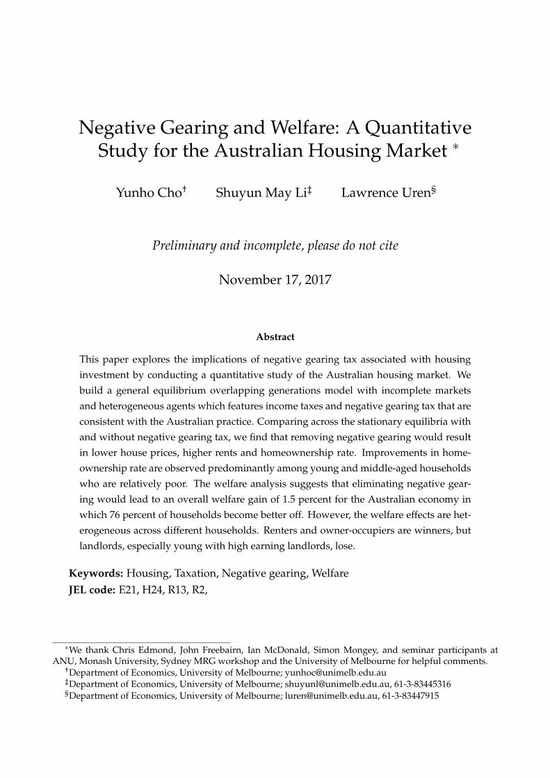
Figure 2 documents the proportion negatively geared landlords and the aggregate net rental

income across the period from 1994 to 2015. The left panel in Figure 2 shows that the pro-

portion of negatively geared landlords has increased from 50 percent in 1994 to around 60

6Another favorable tax treatment to landlords in Australia is 50 percent discount on capital gains tax whichwas introduced in 1999.

7Other on-going expenses on investment properties may include body corporate fees, insurance, propertyagent fees, and maintenance costs.

6

Figure 2: Negatively geared landlords (left) and Net rental income (right)

Source: Taxation Statistics, Table 1 Individual, ATO

percent in 2015. The right panel in Figure 2 shows that the aggregate net rental income

became large negative from the early 2000s onwards. Evidence shown in Figures 1 and 2

suggest that Australian households increasingly participate in the residential property in-

vestment and take advantage of negative gearing, reducing tax obligations with the flow

loss incurred from their housing investment.

Figure 3 compares the share of households with home loans for investment by age (left

panel) and income percentile (right panel) for the years 2002 and 2014. There has been

a significant increase in the share, particularly among young to middle-aged households.

The largest increase was occurred in the age group 25− 35, increased by 85 percent from

7 percent to 13 percent. From the right panel, we find that the share of households with

investment housing loans has increased mainly among those in upper income percentiles.

These evidence are in line with the arguments by opponents of negative gearing that the

policy essentially benefits the rich households who borrow and speculate in the property

market. The fact that the distribution of housing investment loans is different across age

and income also motivates our use of a heterogeneous agents incomplete markets model to

study the implications of negative gearing.

7

Figure 3: Households with investment housing loan: By age (left) and income (right)

Source: Statistical Table E7 – Household Debt Distribution, Reserve Bank of Australia

3 Model

To analyze the effects of negative gearing on the Australian housing market, we develop an

overlapping generations general equilibrium model with heterogeneous agents. The econ-

omy is populated by overlapping generations of households who are subject to uninsurable

idiosyncratic income shocks. Households derive utility from a numeraire non-durable con-

sumption good and housing services, which can be obtained via renting or owning. Home-

owners can purchase additional units of housing stock and lease to other households. The

decision to become a landlord is affected by the government taxation policy. Purchasing and

selling housing stocks incur non-convex transaction costs and homeowners are required to

pay maintenance costs to prevent housing stocks from depreciation. In every period, the

equilibrium price and rent are determined by the market clearing conditions for the hous-

ing and rental markets. A competitive construction sector adjusts the supply of new housing

stocks in response to changes in prices.

8

3.1 Households

Demographics. The economy is populated by a continuum of finitely-lived households

who live and work for a = 1, 2, ..., A periods. Throughout the life-cycle, households face an

age-dependent survival rate of κa, and they all die with certainty after period A.

Preferences. Households derive utility from consumption of non-durables c and housing

services h. The expected lifetime utility of the household is given by:

E0

[A

∑a=1

βa−1κaua(ca, ha)

](1)

with β > 0. The periodic utility of household is given by:

u(c, h) =

[cα(λh)1−α

]1−σ

1− σ(2)

where α denotes preference for non-durables and σ is a risk aversion coefficient. Since there

may be additional utility from living in an owned home, we assume that homeowners re-

ceive premium of λ, with λ > 1 for homeowners and λ = 1 for renters.

A household who dies unexpectedly has all his assets, taken by the government and

liquidated if needed. After settling outstanding debt, the remaining assets are distributed

equally to every surviving household in the economy.

Endowment. A household i with age a supplies a unit of labor inelastically and receives an

income of yi,a. The process of earnings is expressed as:

log yi,a = ηa + zi,a (3)

where ηa is a deterministic component of income that depends on households’ age and zi,a

9

is a persistent idiosyncratic component, which follows an AR(1) process as below:

zi,a = ρzi,a−1 + ui,a ui,a ∼ N(0, σ2u) (4)

The idiosyncratic income shock is the main source of household heterogeneity in our model.

It generates a dispersion of households within and across age groups. This allows us to com-

pare the extensive margin of housing tenure and investment decision among households.

The idiosyncratic income shock is also important for generating the life-cycle savings pat-

terns observed in the data as it creates a precautionary savings motive.

Housing arrangements. The housing asset is denoted by h, available in K discrete sizes.

Households may not choose to purchase a house (h = 0) in which case they obtain housing

services via renting (hrent > 0). Homeowners obtain housing services from a house they

purchased (hown > 0). The amount of housing services consumed is given by:

h =

hrent if renter

hown if owner-occupier

Renters are allowed to live in units smaller than the minimum house size available to

owner-occupiers.8 They can also rent any of larger sizes. Households can become landlords

by purchasing more housing units than they consume (h − h > 0) but cannot derive util-

ity from it. For a given housing size, homeowners can freely switch their dwelling from

owner-occupied houses to investment properties (or vice versa). By assumption, we do not

allow homeowners to consume more housing services than what they purchased in which

case they would become net renters. We also prevent renters from purchasing investment

properties, i.e. no renter-landlords.9

Maintenance and transaction costs. Homeowners incur maintenance expenses, which

8One can think of these units as studio apartments or shared rooms.9In the data, approximately 3 percent of the population are renters who are also landlords.

10

is linear in the housing value, in order to offset physical depreciation of housing stocks.

We use δ to denote any costs associated with maintenance of housing stocks. In addition,

landlords incur an additional fixed cost ζ which captures a cost related to finding tenants

and managing rental property.

Houses are costly to buy and sell. Households face transaction costs of φb percent of

the house value when buying a house and φs percent when selling a house. Thus, the total

transaction costs for buying and selling a house are φb ph and φs ph−1. The presence of trans-

action costs generates sizable inaction regions with respect to the household decision to buy

or sell. We use TC(h−1, h) to describe transaction costs associated with owner-occupied and

investment housing. They are expressed as:

TC(h−1, h) =

0 if h−1 = h

φb ph + φs ph−1 if h−1 6= h

These transaction costs are a dead-weight loss for the economy.10

Borrowing and saving. Households have access to a risk-free asset, s′ that pays interest

r. In any period, a household can save by purchasing this risk-free asset in which case

s′ will be positive. He can also borrow in which case s′ becomes negative. The market

incompleteness implies that households can only borrow using housing stocks as collateral

and the borrowing requires the downpayment of θph. The constraint on s′ is expressed as:

s′ ≥ −(1− θ)ph (5)

If the household is a borrower, he needs to pay mortgage premium of m. We also assume

that the model hinges on a small open economy so that the interest rate r is exogenous.

Housing price risk. To introduce ex-post capital gain or loss from housing investment, we

10The stamp duties are collected by the State government in Australia.

11

introduce an idiosyncratic housing price shock, following Chambers, Garriga, and Schla-

genhauf (2009a,b). The decision to sell housing assets results in households being subject

to an idiosyncratic house price shock, ω ∈ Ω, that influences the final selling price of a

house. Although the selling price may be higher (lower) when a positive (negative) shock

is realized, the stationary equilibrium is preserved as the ex-ante expected capital gain is

zero, i.e. E(ωp) = p. Households have no information of about this i.i.d. shock until the

house is sold, but they know the unconditional probability of the shock which is given by

πω. To avoid the complication of households buying housing assets at different prices, we

assume that the competitive construction firm (to be described later) buys from all selling

households (at different prices) and sells to all purchasing households at a constant price p.11

Taxation and transfers. Households pay tax on labor income, capital income and the net

rental income (NRI), which is defined as:

NRI ≡ (pr − pδ)(h− h)1h>h + (r + m)s(

h− hh

)1h>h∧s<0 − ζ1h>h (6)

The first term on the RHS is rental receipts after paying maintenance costs. The last term

is the periodic fixed cost associated with being a landlord, where 1h>h is an indicator for

landlords. In the second term, (r + m)s is the total interest payments on mortgages, h−hh is

the proportion of investment to total housing stocks owned by a landlord, and 1h>h∧s<0 is

an indicator for landlords with mortgages. The second term therefore represents the mort-

gage interest payments for investment properties. Here, we make a simplifying assumption

that mortgages for investment properties and owner-occupied properties charge the same

interest rate and they are amortized at the same rate.12

11The construction firm can sell houses at a constant price since on average it will make zero capital gainsfrom the sales.

12In real-life, some landlords would payoff mortgages for owner-occupied houses first and leave behindthose for investment housing to maximize tax deductions. Distinguishing mortgages between owner-occupiedand investment housing would require another state variable which puts additional computational burden insolving the model.

12

Accordingly, the total taxable income is expressed as:

Y = ya + rs1s>0 + NRI (7)

which suggests that, if a housing investor is making a loss from his housing investment, i.e.

NRI < 0, he can reduce the amount of taxable income. The total tax payment is represented

by T(Y), which we describe the exact details in Section 3.2. In the baseline economy, the

taxable income is expressed according to (7). In Section 5, we run a counter-factual policy

experiment by setting the taxable income as below:

Y = ya + rs1s>0 + NRI1NRI>0 (8)

This suggests that landlords would have a higher taxable income when they make a positive

profit from housing investment but cannot reduce the income when a loss is realized.

Households receive lump-sum transfers, F, which the government finances through tax-

ation and liquidating the assets of households who unexpectedly die. We can now express

the budget constraint for a household in an arbitrary policy regime as follow:

c + s′ + ph + TC(h−1, h) + T(Y) + ζ1h>h = ya + pω(1− δ)h−1 + pr(h− h)

+ (1 + r + m1s<0)s + F (9)

3.1.1 Household Dynamic Programming Problem

In each period, given price, rent and transfer payment (p, pr, F), households choose whether

(i) to rent, or (ii) to own a house. If they decide to own, they also decide upon investment in

housing. Household’s current state comprises of four individual variables: housing assets

h−1, savings s, the current realization of idiosyncratic income shock z, and household’s age

a. For notational convenience, we group these state variables into x ≡ (a, s, h−1, z). The

13

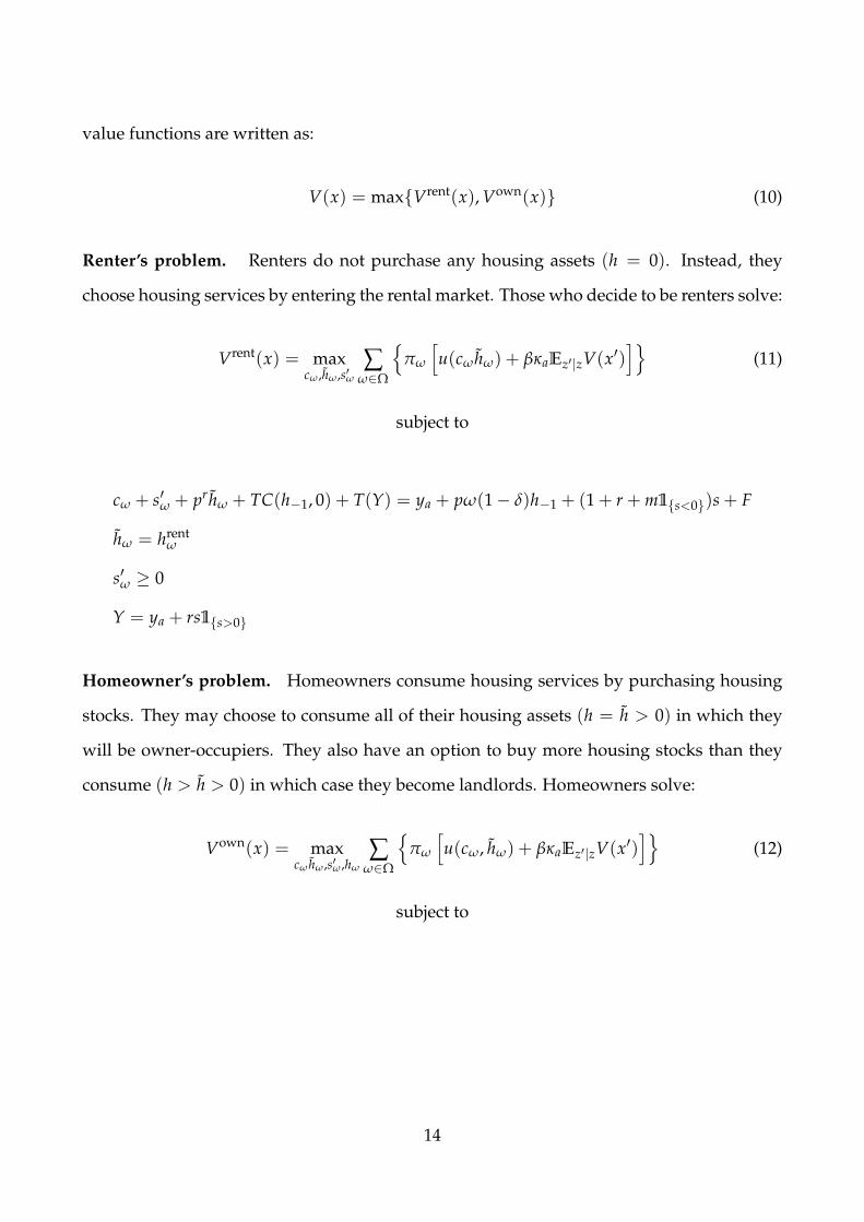
value functions are written as:

V(x) = maxVrent(x), Vown(x) (10)

Renter’s problem. Renters do not purchase any housing assets (h = 0). Instead, they

choose housing services by entering the rental market. Those who decide to be renters solve:

Vrent(x) = maxcω ,hω ,s′ω

∑ω∈Ω

πω

[u(cω hω) + βκaEz′|zV(x′)

](11)

subject to

cω + s′ω + pr hω + TC(h−1, 0) + T(Y) = ya + pω(1− δ)h−1 + (1 + r + m1s<0)s + F

hω = hrentω

s′ω ≥ 0

Y = ya + rs1s>0

Homeowner’s problem. Homeowners consume housing services by purchasing housing

stocks. They may choose to consume all of their housing assets (h = h > 0) in which they

will be owner-occupiers. They also have an option to buy more housing stocks than they

consume (h > h > 0) in which case they become landlords. Homeowners solve:

Vown(x) = maxcω hω ,s′ω ,hω

∑ω∈Ω

πω

[u(cω, hω) + βκaEz′|zV(x′)

](12)

subject to

14

cω + s′ω + phω + TC(h−1, hω) + T(Y) + ζ1hω>hω = ya + pω(1− δ)h−1 + pr(hω − hω)

+ (1 + r + m1s<0)s + F

hω = hownω

s′ω ≥ −(1− θ)phω

Y = ya + rs1s>0 + NRI

where NRI is given by (6). Notice that all choice variables are now indexed by ω since

households’ choice depends on the realization of the i.i.d. house price shock upon the sales

of housing assets.

3.2 Government

This section provides a parsimonious representation of the Australian tax system in which

households’ taxable income is taxed at different marginal rates. The total amount of taxation

imposed on households is determined by

T(Y) =

0 if Y ≤ Y1

τ1(Y− Y1) if Y1 < Y ≤ Y2

T1 + τ2(Y− Y2) if Y2 < Y ≤ Y3

...

TQ−2 + τQ−1(Y− YQ) if YQ−1 < Y ≤ YQ

where Yqs are income thresholds, τq is the marginal tax rates, Tq is the tax payment thresh-

old. It is assumed that Tq = Tq−1 + τq(Yq+1 − Yq).

Apart from taxation, the government finances its spending by selling the wealth of de-

ceased households. Each period, the government sells housing stocks owned by those who

die unexpectedly and pays off any outstanding debt. We use the letter R to denote these

residual wealth collected by the government. The government spends all of its revenue by

distributing lump-sum transfers equally to living households, denoted by F. A household

15

who dies unexpectedly therefore leaves accidental bequests. The presence of lump-sum

transfers is important for redistributive channels as a reform that increases government’s

taxation revenue may benefit young and poor households in the counterfactual economy

as lump-sum transfer would increase. The government runs a balanced budget in every

period.

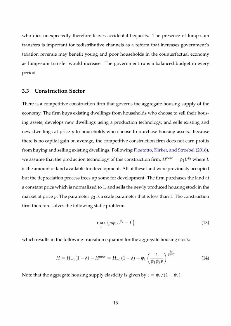
3.3 Construction Sector

There is a competitive construction firm that governs the aggregate housing supply of the

economy. The firm buys existing dwellings from households who choose to sell their hous-

ing assets, develops new dwellings using a production technology, and sells existing and

new dwellings at price p to households who choose to purchase housing assets. Because

there is no capital gain on average, the competitive construction firm does not earn profits

from buying and selling existing dwellings. Following Floetotto, Kirker, and Stroebel (2016),

we assume that the production technology of this construction firm, Hnew = ψ1Lψ2 where L

is the amount of land available for development. All of these land were previously occupied

but the depreciation process frees up some for development. The firm purchases the land at

a constant price which is normalized to 1, and sells the newly produced housing stock in the

market at price p. The parameter ψ2 is a scale parameter that is less than 1. The construction

firm therefore solves the following static problem:

maxL

pψ1Lψ2 − L

(13)

which results in the following transition equation for the aggregate housing stock:

H = H−1(1− δ) + Hnew = H−1(1− δ) + ψ1

(1

ψ1ψ2p

) ψ2ψ2−1

(14)

Note that the aggregate housing supply elasticity is given by ε = ψ2/(1− ψ2).

16

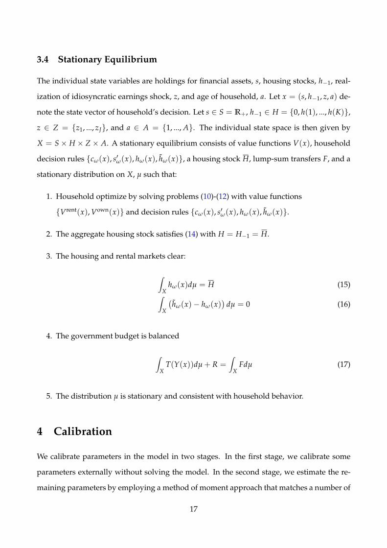
3.4 Stationary Equilibrium

The individual state variables are holdings for financial assets, s, housing stocks, h−1, real-

ization of idiosyncratic earnings shock, z, and age of household, a. Let x = (s, h−1, z, a) de-

note the state vector of household’s decision. Let s ∈ S = R+, h−1 ∈ H = 0, h(1), ..., h(K),

z ∈ Z = z1, ..., zJ, and a ∈ A = 1, ..., A. The individual state space is then given by

X = S× H × Z× A. A stationary equilibrium consists of value functions V(x), household

decision rules cω(x), s′ω(x), hω(x), hω(x), a housing stock H, lump-sum transfers F, and a

stationary distribution on X, µ such that:

1. Household optimize by solving problems (10)-(12) with value functions

Vrent(x), Vown(x) and decision rules cω(x), s′ω(x), hω(x), hω(x).

2. The aggregate housing stock satisfies (14) with H = H−1 = H.

3. The housing and rental markets clear:

∫X

hω(x)dµ = H (15)∫X

(hω(x)− hω(x)

)dµ = 0 (16)

4. The government budget is balanced

∫X

T(Y(x))dµ + R =∫

XFdµ (17)

5. The distribution µ is stationary and consistent with household behavior.

4 Calibration

We calibrate parameters in the model in two stages. In the first stage, we calibrate some

parameters externally without solving the model. In the second stage, we estimate the re-

maining parameters by employing a method of moment approach that matches a number of

17

model moment from the baseline steady state to their data counterpart as close as possible.

We summarize parameters that externally determined in Table 1 and estimated parameters

and respective moments in Table 2.

4.1 Externally Calibrated Parameter Values

Demographics. The model period is set to 5 years. Households enter the model at age

21 and exit at age 90. Thus, the number of age cohorts is 14. The age dependent survival

probability, κa, is obtained from the ABS Life Table 2007− 2009.

Preferences. The coefficient of risk aversion, σ is set to 2, which is a standard value in

macroeconomics. Other parameters in the utility function, α and λ are calibrated internally

via estimation.

Endowments. The endowment process is estimated using the age and income data in the

Household Labour Income Dynamics Australia (HILDA). To be consistent with the model,

we construct the exogenous income by subtracting the investment income (e.g. savings

and rental income) from the total gross income. Accordingly, our income measure captures

households’ gross income that includes pensions and transfers but excludes any investment

income. We extract the deterministic component, ηaA=14a=1 from a fourth order polynomi-

als in age cohort. This component explains the life-cycle earnings profile that is increasing

(decreasing) during the earlier (later) stages of life. The stochastic component of earnings,

zi,a, is estimated to follow an AR(1) process with persistence of 0.65 and standard deviation

for innovations of 0.45.13 We provide a detailed description of the estimation of the earnings

process in Appendix. We discretize a continuous process of earnings into five states using

the method of Tauchen and Hussey (1991).14 The median income in our model is estimated

13These are the 5-year values converted using the annual estimates of ρ = 0.94 and σ2u = 0.03. See Appendix

for our approach to conversion of the annual value to the 5-year value.14We also apply a weighting function proposed by Floden (2008) that corrects for the critique of Tauchen

and Hussey (1991) with a highly persistence process.

18

to be $347,800 which is used to normalize other variables in monetary units.

Housing. The transaction costs for buyers come from the weighted average stamp duty for

seven capital cities from 2001 to 2014 which is about 3.75 percent of the purchase price, so

we set φb = 0.0375. The transaction cost for sellers is set φs = 0.03 which corresponds to

the average real-estate agent fee of 3 percent of the selling price. The maintenance cost is set

to offset depreciation. In the SIH 2013-14, we find that homeowners pay maintenance ex-

penses around 2.2 percent of the housing value. This is similar to those reported in the U.S.

studies.15. Given that, we set δ = 0.02 per year. This translates to the model value of 0.104.

The downpayment requirement, θ, is set at 0.2, consistent with the practice in Australia and

other advanced economies. The minimum size for owner-occupied housing, h(1) is set to

be 80 percent of the model’s median income.

Interest rates. The interest paid on the risk-free asset is calibrated from the average yield

of the 5-year maturity Commonwealth government bond across January 2001 to December

2015, deflated by annual CPI inflation. This gives us the real interest rate of 1.66 percent

per annum, equivalent to the model value of 9.2 percent. The annual mortgage premium

is calculated by subtracting the risk-free rate from the real variable lending rates for owner-

occupied housing across the same period. The annual average is 2.26 percent which trans-

lates to the model value of 11.8 percent. These rates are all obtained from the Reserve Bank

of Australia.

Taxation. The income tax function captures the progressivity of the Australian tax system.

The parameters to be calibrated are income thresholds for each tax bracket Yq, the marginal

tax rates τq, and the tax payment thresholds for each bracket, Tq. These are obtained from

the Australian Taxation Office using the income tax system for the 2012-13 financial year.

The function is given by:

15For example, Floetotto, Kirker, and Stroebel (2016) reports δ = 0.02 and Sommer and Sullivan (2016) setδ = 0.015.

19

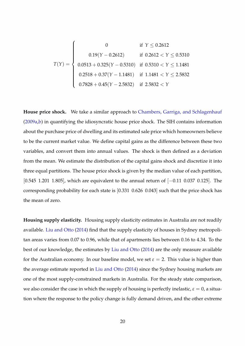
T(Y) =

0 if Y ≤ 0.2612

0.19(Y− 0.2612) if 0.2612 < Y ≤ 0.5310

0.0513 + 0.325(Y− 0.5310) if 0.5310 < Y ≤ 1.1481

0.2518 + 0.37(Y− 1.1481) if 1.1481 < Y ≤ 2.5832

0.7828 + 0.45(Y− 2.5832) if 2.5832 < Y

House price shock. We take a similar approach to Chambers, Garriga, and Schlagenhauf

(2009a,b) in quantifying the idiosyncratic house price shock. The SIH contains information

about the purchase price of dwelling and its estimated sale price which homeowners believe

to be the current market value. We define capital gains as the difference between these two

variables, and convert them into annual values. The shock is then defined as a deviation

from the mean. We estimate the distribution of the capital gains shock and discretize it into

three equal partitions. The house price shock is given by the median value of each partition,

[0.545 1.201 1.805], which are equivalent to the annual return of [−0.11 0.037 0.125]. The

corresponding probability for each state is [0.331 0.626 0.043] such that the price shock has

the mean of zero.

Housing supply elasticity. Housing supply elasticity estimates in Australia are not readily

available. Liu and Otto (2014) find that the supply elasticity of houses in Sydney metropoli-

tan areas varies from 0.07 to 0.96, while that of apartments lies between 0.16 to 4.34. To the

best of our knowledge, the estimates by Liu and Otto (2014) are the only measure available

for the Australian economy. In our baseline model, we set ε = 2. This value is higher than

the average estimate reported in Liu and Otto (2014) since the Sydney housing markets are

one of the most supply-constrained markets in Australia. For the steady state comparison,

we also consider the case in which the supply of housing is perfectly inelastic, ε = 0, a situa-

tion where the response to the policy change is fully demand driven, and the other extreme

20

Table 1: Externally Chosen Parameter Values

Parameter Model value Annual value Sourcer Risk-free interest rate 0.092 0.018 RBAm Mortgage premium 0.118 0.023 RBAσ Coefficient of risk aversion 2 Literatureφb Trans. cost for buyer (frac. house value) 0.037 Ave. stamp dutyφs Trans. cost for seller (frac. house value) 0.03 Ave. agent feeδ Depreciation of housing stock 0.104 0.02 SIHρ Persistence of income process 0.65 0.94 HILDAσu Std. dev. of income innovation 0.44 0.173 HILDA

h(1) Minimum housing size for purchase 0.8ε Housing supply elasticity 2ω Capital gain shock (annual) [−0.114 0.037 0.125] SIHκa Survival probability (age-dependent) ABS

Yk, τk, Tk Taxation Refer to text ATO

where housing supply is highly elastic, ε = 6.16

4.2 Calibration via Estimation

The remaining parameters, Θ = ζ, β, λ, α, are calibrated jointly through model estimation.

We estimate these parameters using the method of moments approach that matches the

model’s equilibrium moments with the empirical moments constructed from the SIH and

the HILDA survey. The procedure we use is briefly summarized as follows:

Let Mj represents the jth moment in the data, and let Mj(Θ) represent the corresponding

moments generated by the model equilibrium. The task is to find Θ that minimizes the

following objective function:

L(Θ) = arg minΘ

J

∑j=1

(Mj −Mj(Θ)

)′W (Mj −Mj(Θ)

)(18)

where W is an identity matrix. Minimizing this function requires solving the household’s

optimization problem and finding equilibrium house price and rent for each trial value of

the parameter vector. The solution to (18) is a vector of parameters Θ = ζ, β, λ, α that

are jointly estimated by minimizing the distance between M and M(Θ). Below, we describe

16Housing supply will often be inelastic at least in the short-run due to restrictions such as land constraintsand regulation.

21

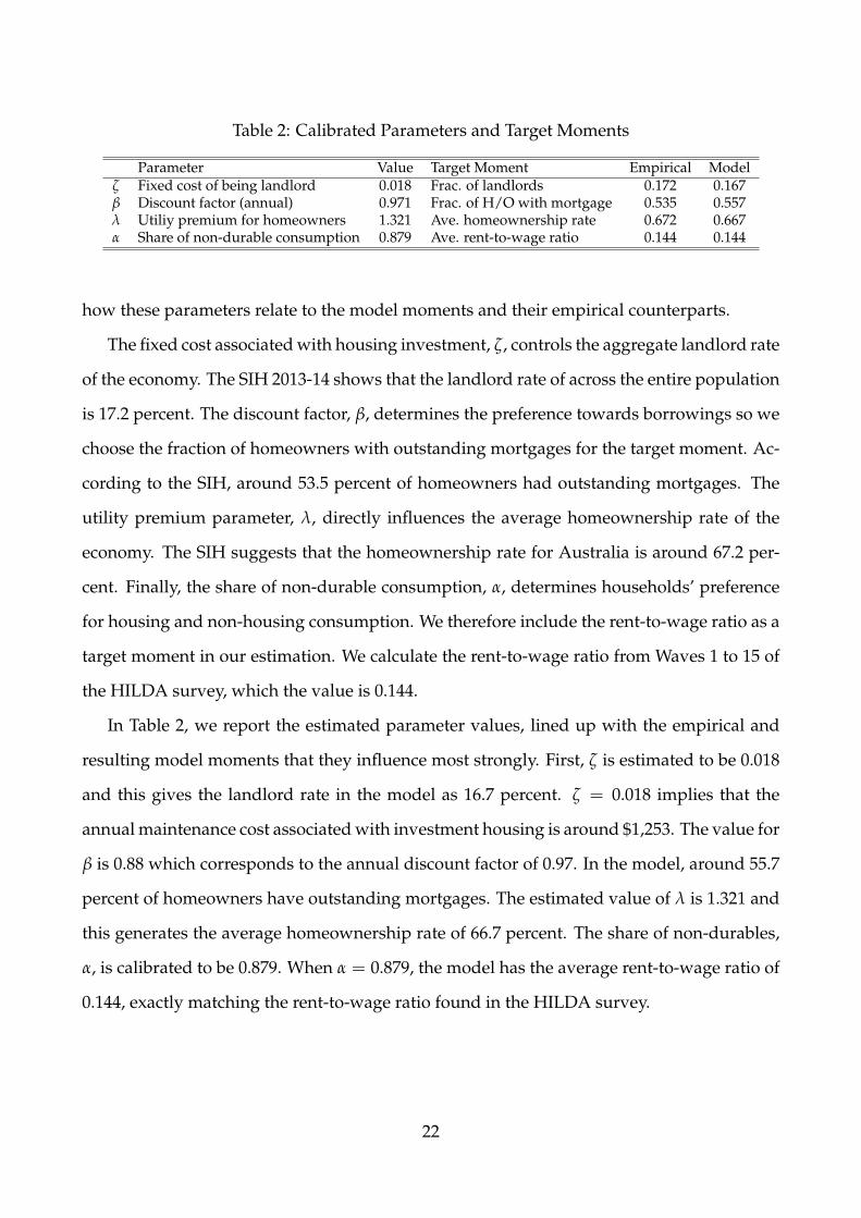
Table 2: Calibrated Parameters and Target Moments

Parameter Value Target Moment Empirical Modelζ Fixed cost of being landlord 0.018 Frac. of landlords 0.172 0.167β Discount factor (annual) 0.971 Frac. of H/O with mortgage 0.535 0.557λ Utiliy premium for homeowners 1.321 Ave. homeownership rate 0.672 0.667α Share of non-durable consumption 0.879 Ave. rent-to-wage ratio 0.144 0.144

how these parameters relate to the model moments and their empirical counterparts.

The fixed cost associated with housing investment, ζ, controls the aggregate landlord rate

of the economy. The SIH 2013-14 shows that the landlord rate of across the entire population

is 17.2 percent. The discount factor, β, determines the preference towards borrowings so we

choose the fraction of homeowners with outstanding mortgages for the target moment. Ac-

cording to the SIH, around 53.5 percent of homeowners had outstanding mortgages. The

utility premium parameter, λ, directly influences the average homeownership rate of the

economy. The SIH suggests that the homeownership rate for Australia is around 67.2 per-

cent. Finally, the share of non-durable consumption, α, determines households’ preference

for housing and non-housing consumption. We therefore include the rent-to-wage ratio as a

target moment in our estimation. We calculate the rent-to-wage ratio from Waves 1 to 15 of

the HILDA survey, which the value is 0.144.

In Table 2, we report the estimated parameter values, lined up with the empirical and

resulting model moments that they influence most strongly. First, ζ is estimated to be 0.018

and this gives the landlord rate in the model as 16.7 percent. ζ = 0.018 implies that the

annual maintenance cost associated with investment housing is around $1,253. The value for

β is 0.88 which corresponds to the annual discount factor of 0.97. In the model, around 55.7

percent of homeowners have outstanding mortgages. The estimated value of λ is 1.321 and

this generates the average homeownership rate of 66.7 percent. The share of non-durables,

α, is calibrated to be 0.879. When α = 0.879, the model has the average rent-to-wage ratio of

0.144, exactly matching the rent-to-wage ratio found in the HILDA survey.

22

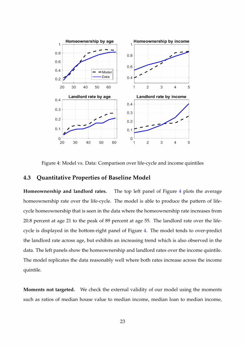
Figure 4: Model vs. Data: Comparison over life-cycle and income quintiles

4.3 Quantitative Properties of Baseline Model

Homeownership and landlord rates. The top left panel of Figure 4 plots the average

homeownership rate over the life-cycle. The model is able to produce the pattern of life-

cycle homeownership that is seen in the data where the homeownership rate increases from

20.8 percent at age 21 to the peak of 89 percent at age 55. The landlord rate over the life-

cycle is displayed in the bottom-right panel of Figure 4. The model tends to over-predict

the landlord rate across age, but exhibits an increasing trend which is also observed in the

data. The left panels show the homeownership and landlord rates over the income quintile.

The model replicates the data reasonably well where both rates increase across the income

quintile.

Moments not targeted. We check the external validity of our model using the moments

such as ratios of median house value to median income, median loan to median income,

23

Table 3: Moments not Targeted

Moment Data ModelHouse value to Income Ratio 1.37 1.25

Loan to Income Ratio 0.67 0.69Loan to Value Ratio 0.49 0.65

Proportion of negatively geared landlords 0.64 0.70

Note: The first three rows of the data column are sourced from SIH 2013-14. The proportion of negativelygeared landlords is sourced from Taxation Statistics from 2001 to 2015.

and median loan to median house value ratio. We report the empirical counterparts from the

SIH. These moments are not targeted in our estimation. Table 3 shows that the model pro-

duces very similar values for these moments to their empirical counterparts. Importantly,

the last row of Table 3 shows that the model is able to match the average proportion of nega-

tively geared landlords reported in ATO’s Taxation Statistics between 2001 and 2012. Given

our research question, it is crucial to generate a significant number of negatively geared

landlords in equilibrium. What drives the proportion of negatively geared landlords? It is

the capital gains that outweighs the flow loss incurred during investment periods. In our

model, we introduce an i.i.d. capital gains shock that allows many homeowners to receive

capital gains upon sales. Although the ex-ante expected capital gains is zero, most housing

investments generate capital gains ex-post, playing a central role in generating a positive

proportion of negatively geared households. The fact the model is able to match this gives

additional credibility to our calibration strategy discussed in this section.

5 Removing Negative Gearing

In this section, we present the main result of this paper, the effects of negative gearing on

housing price, rent, homeownership rate and household welfare. We do so by comparing the

equilibrium outcomes of the baseline economy with that of a counterfactual economy which

does not feature negative gearing. The baseline economy is solved with taxes and the taxable

income, given by (7). The net rental income in the counterfactual economy follows (8) in

24

Table 4: Steady state comparison

Baseline No NGε = 2 ε = 0 ε = 6

Price 1.180 1.160 1.138 1.168Rent 0.164 0.168 0.169 0.168Price-rent ratio 7.209 6.907 6.725 6.947Frac. of homeowners 0.667 0.722 0.750 0.721Frac. of owner-occupiers 0.500 0.584 0.591 0.578Frac. of landlords 0.167 0.138 0.158 0.143Frac. of renters 0.333 0.242 0.250 0.279Ave. mortgage size 0.936 0.712 0.710 0.754Debt to income ratio 0.356 0.304 0.300 0.301Ave. expenditure: investment housing 1.676 1.386 1.365 1.405Frac. of negatively geared investors 0.701 0.505 0.459 0.506Transfers 0.229 0.236 0.234 0.237Rental supply (relative to housing supply) 0.263 0.184 0.211 0.192Housing supply (normalized) 1 0.987 1 0.949

Note: The last two columns provide results for the reformed economy using alternative values of housingsupply elasticity, ε = 0 and ε = 6. With inelastic housing supply, the price of housing declines by more sincethere is no supply response. The homeownership rate in the inelastic economy is higher because theprice-to-rent ratio is lower. With a higher elasticity, the price declines by less because the housing supplydecreases more than the economy with ε = 2. Other moments of the model are hardly affected by theelasticity.

which landlords are no longer allowed to reduce the total taxable income when negative

per-period rental income is realized.

5.1 Steady State

Table 4 compares the effects of negative gearing on house prices, rents and other aggregate

statistics across steady states. When negative gearing is repealed, housing prices decrease

by 1.7 percent while rents increase by 2.4 percent. The housing prices fall because remov-

ing negative gearing takes a significant amount of housing investment out of the property

market. Both the proportion of landlords and the amount of resources allocated to hous-

ing investment, given by the average expenditure, have fallen significantly after the policy

reform. The rent rises mainly because there is a decline in the aggregate supply of rental

properties which decreased more than 30 percent relative to that in the baseline economy.

Importantly, removing negative gearing increases the average homeownership rate of

the economy from 66.7 percent to 72.2 percent. We provide the following mechanisms for

25

Table 5: Changes in homeownership and owner-occupier rates (difference in % points)

∆ in homeownership rate ∆ in owner-occupier rateAge Income QuintileGroup Q1 Q2 Q3 Q4 Q5 Q1 Q2 Q3 Q4 Q535 or below 1.36 1.73 -1.48 -0.31 6.94 1.48 5.48 4.81 11.61 12.1636− 50 9.60 7.32 6.67 1.80 1.45 10.44 10.85 13.34 6.47 19.4851− 65 6.59 7.02 2.22 2.34 1.81 6.85 4.10 2.59 3.38 10.2466 or above 12.33 6.73 8.41 4.78 4.51 8.37 5.73 9.90 7.31 10.42

this. The fall in house price and the rise in rent reduce the price-to-rent ratio in the econ-

omy. In our simulation, the ratio falls by 4.2 percent. This has direct implications on housing

affordability as the fall in house price lowers both the downpayment requirement for mort-

gages and the size of mortgages required to purchase a house, making it easier for house-

holds to own a home. The simulation suggests that the average size of mortgages held by

homeowners decreases by 21 percent. Moreover, the transaction costs associated with sell-

ing and buying housing stocks decrease with the lower purchasing price. On the other hand,

the rise in rents promotes renters to become homeowners as it increases the cost of renting.

The improvement in homeownership is observed most predominantly among poor house-

holds. The impact of the policy change on home affordability is largest for these households

because the lower housing price and higher lump-sum transfer allow those poor households

who were at the margin of being homeowners to achieve housing tenure. In Table 5, we re-

port the percentage point change in homeownership and owner-occupier rates by age group

and income quintile. For the sake of exposition, we group age cohorts into four categories

including 35 or below, 36− 50, 51− 65, and 66 or above. Eliminating negative gearing in-

creases the homeownership rate for most groups of households. Note that negative values

shown in the left half of Table 5 (changes in homeownership rate) are driven by landlords

who decide to become renters after the policy change. As shown in the right half of Table

5, the owner-occupier rate increases ubiquitously for all age groups and income quintiles.

In particular, such an increase is most prominent for households who were relatively young

and poor. For instance, the homeownership rate for the age group under 35 and the lowest

26

Figure 5: Baseline vs. No negative gearing: Comparison over life-cycle and income quintiles

income quintile increase by 26.4 percent (1.4 percentage points). Also, the owner-occupier

rates for the age group under 35 and the first and second income quintiles increases 60 per-

cent (1.5 percentage points) and 104 percent (5.8 percentage points) respectively. We also

find that these changes are greater for young and mid-aged households. The top right panel

of Figure 5 also shows that the homeownership rate for the lower income quintiles increased

proportionately more than that experienced by households at higher income quintiles.

How does housing allocation shift between high and low income households? To an-

swer this question, we look at the percentage change in housing services consumption and

the purchase of housing assets for households at each income quintile. The allocation of

housing stocks shifts from the high income to low income households. Figure 6 shows that

consumption for housing services improves for every income quintile. For instance, in the

counter-factual steady state, households in the first income quintile consume housing ser-

vices around 9 percent more relative to the baseline steady state. Similarly, the aggregate

housing stocks purchased by those households in the counter-factual economy is around 17

27

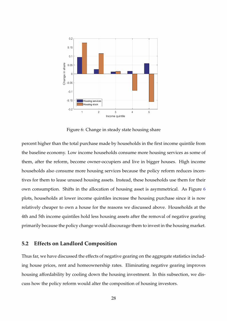
Figure 6: Change in steady state housing share

percent higher than the total purchase made by households in the first income quintile from

the baseline economy. Low income households consume more housing services as some of

them, after the reform, become owner-occupiers and live in bigger houses. High income

households also consume more housing services because the policy reform reduces incen-

tives for them to lease unused housing assets. Instead, these households use them for their

own consumption. Shifts in the allocation of housing asset is asymmetrical. As Figure 6

plots, households at lower income quintiles increase the housing purchase since it is now

relatively cheaper to own a house for the reasons we discussed above. Households at the

4th and 5th income quintiles hold less housing assets after the removal of negative gearing

primarily because the policy change would discourage them to invest in the housing market.

5.2 Effects on Landlord Composition

Thus far, we have discussed the effects of negative gearing on the aggregate statistics includ-

ing house prices, rent and homeownership rates. Eliminating negative gearing improves

housing affordability by cooling down the housing investment. In this subsection, we dis-

cuss how the policy reform would alter the composition of housing investors.

28

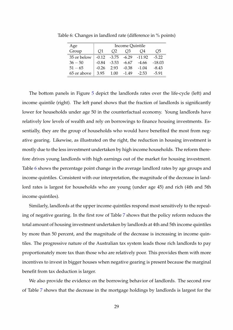
Table 6: Changes in landlord rate (difference in % points)

Age Income QuintileGroup Q1 Q2 Q3 Q4 Q535 or below -0.12 -3.75 -6.29 -11.92 -5.2236− 50 -0.84 -3.53 -6.67 -4.66 -18.0351− 65 -0.26 2.93 -0.38 -1.04 -8.4365 or above 3.95 1.00 -1.49 -2.53 -5.91

The bottom panels in Figure 5 depict the landlords rates over the life-cycle (left) and

income quintile (right). The left panel shows that the fraction of landlords is significantly

lower for households under age 50 in the counterfactual economy. Young landlords have

relatively low levels of wealth and rely on borrowings to finance housing investments. Es-

sentially, they are the group of households who would have benefited the most from neg-

ative gearing. Likewise, as illustrated on the right, the reduction in housing investment is

mostly due to the less investment undertaken by high income households. The reform there-

fore drives young landlords with high earnings out of the market for housing investment.

Table 6 shows the percentage point change in the average landlord rates by age groups and

income quintiles. Consistent with our interpretation, the magnitude of the decrease in land-

lord rates is largest for households who are young (under age 45) and rich (4th and 5th

income quintiles).

Similarly, landlords at the upper income quintiles respond most sensitively to the repeal-

ing of negative gearing. In the first row of Table 7 shows that the policy reform reduces the

total amount of housing investment undertaken by landlords at 4th and 5th income quintiles

by more than 50 percent, and the magnitude of the decrease is increasing in income quin-

tiles. The progressive nature of the Australian tax system leads those rich landlords to pay

proportionately more tax than those who are relatively poor. This provides them with more

incentives to invest in bigger houses when negative gearing is present because the marginal

benefit from tax deduction is larger.

We also provide the evidence on the borrowing behavior of landlords. The second row

of Table 7 shows that the decrease in the mortgage holdings by landlords is largest for the

29

Table 7: Other effects on landlords

Q1 Q2 Q3 Q4 Q5% change in totalhousing investment

-4.89 -2.89 -22.00 -46.24 -64.04by income quintiles% change in landord’smortgage holdings

-16.15 -20.14 -34.54 -53.41 -66.70by income quintiles% change inlandlord rates

-10.76 -11.10 -21.98 -17.47 -21.61by mortgage quintiles

4th and 5th quintiles. The last row of Table 7 supports this result by showing that the fall

in landlord rates is also larger for higher quintiles of mortgage holdings by landlords. The

landlord rates for the 4th and 5th quintiles decrease approximately 1.5 to 2 times more than

that for the first quintile, suggesting that landlords move down along the mortgage quin-

tiles. The policy reform mitigates the borrowing activities of landlords and makes them to

hold less debt than the baseline economy.

These predictions reconcile the recent trend in landlord compositions shown in Section

2 in which the share of households with investment housing loans increased more sharply

for the group of landlords who are young and rich. Our model predicts that such landlords

would respond most sensitively, reducing the amount of mortgage holdings and investing

less in the property market when negative gearing is repealed.

5.3 Welfare Analysis

We now turn to the welfare analysis. Following the existing literature, welfare is measured

using the notion of consumption equivalence variation (CEV).17 In accounting for the mag-

nitude of welfare gain or loss, we calculate the percentage change in the current consump-

tion of non-durable good that equates the expected discounted utility of the counterfactual

17See Conesa, Kitao, and Krueger (2009) and Hong and Ríos-Rull (2012) for a welfare discussion of moregeneral life-cycle models. For the life-cycle housing literature, see Nakajima (2012), Chambers, Garriga, andSchlagenhauf (2009b), and Floetotto, Kirker, and Stroebel (2016) where the authors take a similar approach tothe method used in this paper.

30

economy with that of the baseline economy. In our model, households are heterogeneous

in terms of their financial position, housing assets, age and earnings, as summarized in the

state vector x. So a welfare analysis requires us to find the consumption equivalence vari-

ation for each pair of identical households characterized by a particular x from the baseline

and counterfactual economies. Formally, we solve the cev for each x (and transform them

into percentage changes) such that:

V(x)nong = u(c∗(x) + cev, h∗(x)

)+ βκaEz′|z

[V(x′∗(x))ng] for any x ≡ (a, s, h, z) (19)

where V(x)ng and V(x)nong denote the value functions with and without negative gearing.

So the LHS of (19) is the expected discounted utility of a household in the economy without

negative gearing, and the RHS is that of the same household living in the baseline economy

with c∗(x), h∗(x) and x′∗(x) being the optimal decision rules in the baseline economy. Our

measure of welfare can be interpreted as the percentage change in non-durable consumption

required by a household in the baseline economy to ensure he is as well off as a household

with the same state variables in the reformed economy. A positive value for consumption

equivalence variation suggests that households are better off in the reformed economy, im-

plying that repealing negative gearing improves the welfare. Note that our analysis is based

on the unexpected change in the policy that does not allow households to re-optimize their

decision in future periods.

Removing negative gearing improves the aggregate welfare. Figure 7 displays a kernel

density plot of CEVs across households from the two stationary equilibria. Eliminating

negative gearing generates the average welfare gain of 1.5 percent for the economy. Also, the

median welfare gain is 4.7 percent and around 76 percent of households prefer to live in an

economy without negative gearing. We provide two reasons why welfare improves for the

economy. First, negative gearing is a policy that largely benefits landlords. In our baseline

economy, approximately 17 percent of households are landlords and of those, 70 percent are

negatively geared. This means that less than 13 percent of the entire population are directly

31

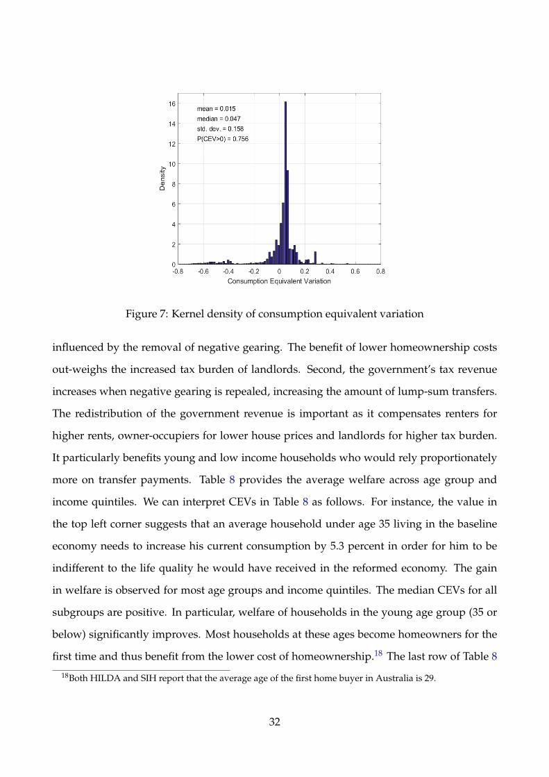
Figure 7: Kernel density of consumption equivalent variation

influenced by the removal of negative gearing. The benefit of lower homeownership costs

out-weighs the increased tax burden of landlords. Second, the government’s tax revenue

increases when negative gearing is repealed, increasing the amount of lump-sum transfers.

The redistribution of the government revenue is important as it compensates renters for

higher rents, owner-occupiers for lower house prices and landlords for higher tax burden.

It particularly benefits young and low income households who would rely proportionately

more on transfer payments. Table 8 provides the average welfare across age group and

income quintiles. We can interpret CEVs in Table 8 as follows. For instance, the value in

the top left corner suggests that an average household under age 35 living in the baseline

economy needs to increase his current consumption by 5.3 percent in order for him to be

indifferent to the life quality he would have received in the reformed economy. The gain

in welfare is observed for most age groups and income quintiles. The median CEVs for all

subgroups are positive. In particular, welfare of households in the young age group (35 or

below) significantly improves. Most households at these ages become homeowners for the

first time and thus benefit from the lower cost of homeownership.18 The last row of Table 8

18Both HILDA and SIH report that the average age of the first home buyer in Australia is 29.

32

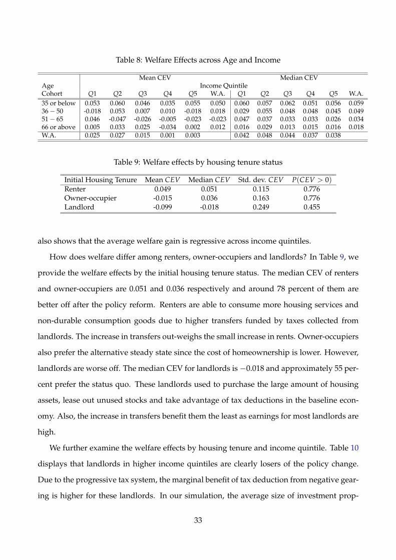
Table 8: Welfare Effects across Age and Income

Mean CEV Median CEVAge Income QuintileCohort Q1 Q2 Q3 Q4 Q5 W.A. Q1 Q2 Q3 Q4 Q5 W.A.35 or below 0.053 0.060 0.046 0.035 0.055 0.050 0.060 0.057 0.062 0.051 0.056 0.05936− 50 -0.018 0.053 0.007 0.010 -0.018 0.018 0.029 0.055 0.048 0.048 0.045 0.04951− 65 0.046 -0.047 -0.026 -0.005 -0.023 -0.023 0.047 0.037 0.033 0.033 0.026 0.03466 or above 0.005 0.033 0.025 -0.034 0.002 0.012 0.016 0.029 0.013 0.015 0.016 0.018W.A. 0.025 0.027 0.015 0.001 0.003 0.042 0.048 0.044 0.037 0.038

Table 9: Welfare effects by housing tenure status

Initial Housing Tenure Mean CEV Median CEV Std. dev. CEV P(CEV > 0)Renter 0.049 0.051 0.115 0.776Owner-occupier -0.015 0.036 0.163 0.776Landlord -0.099 -0.018 0.249 0.455

also shows that the average welfare gain is regressive across income quintiles.

How does welfare differ among renters, owner-occupiers and landlords? In Table 9, we

provide the welfare effects by the initial housing tenure status. The median CEV of renters

and owner-occupiers are 0.051 and 0.036 respectively and around 78 percent of them are

better off after the policy reform. Renters are able to consume more housing services and

non-durable consumption goods due to higher transfers funded by taxes collected from

landlords. The increase in transfers out-weighs the small increase in rents. Owner-occupiers

also prefer the alternative steady state since the cost of homeownership is lower. However,

landlords are worse off. The median CEV for landlords is−0.018 and approximately 55 per-

cent prefer the status quo. These landlords used to purchase the large amount of housing

assets, lease out unused stocks and take advantage of tax deductions in the baseline econ-

omy. Also, the increase in transfers benefit them the least as earnings for most landlords are

high.

We further examine the welfare effects by housing tenure and income quintile. Table 10

displays that landlords in higher income quintiles are clearly losers of the policy change.

Due to the progressive tax system, the marginal benefit of tax deduction from negative gear-

ing is higher for these landlords. In our simulation, the average size of investment prop-

33

Table 10: Welfare effects by housing tenure status and income quintiles

Median CEV P(CEV > 0)Initial Housing Income QuintileTenure Q1 Q2 Q3 Q4 Q5 Q1 Q2 Q3 Q4 Q5Renter 0.059 0.057 0.051 0.049 0.053 0.812 0.782 0.732 0.915 0.944Owner-occupier 0.025 0.036 0.036 0.037 0.039 0.672 0.704 0.782 0.788 0.858Landlord 0.027 0.009 -0.014 -0.072 -0.363 0.718 0.544 0.475 0.374 0.106

Table 11: Welfare effects by housing tenure status and age group

Median CEV P(CEV > 0)Age Initial Housing Tenure StatusGroup Renter Owner-occupier Landlord Renter Owner-occupier LandlordUnder 35 0.056 0.056 -0.092 0.777 0.808 0.28636− 50 0.051 0.048 -0.081 0.794 0.841 0.41851− 65 0.049 0.033 -0.018 0.846 0.768 0.448Above 66 0.024 0.013 0.030 0.689 0.675 0.664

erties purchased by landlords in the fourth and fifth income quintiles decrease by 29 and

41 percent which are much higher than that of landlords in other income quintiles. Scrap-

ping the tax concession disincentivizes rich landlords from housing investment and make

them worse off. On the other hand, landlords at lower income quintiles prefer to live in

the reformed economy because they face lower marginal tax rates so that the gains from an

increase in rental receipts and higher transfer payments exceed the loss from the tax conces-

sion.

Finally, we provide the welfare effects across housing tenure and age group in Table 11.

The biggest welfare loss occurs for landlords who are relatively young. The median CEV

for landlords who are under 35 is -0.082 while that of those between age 35− 50 is -0.081,

and around 71 and 58 percent of young landlords in those two age groups suffer from the

welfare loss. The young landlords are worse off because most of them rely on borrowings

and incur rental loss during the earlier stage of their housing investment. Essentially, they

are the group of households who would have benefited the most from negative gearing. As

displayed in Figure 8, landlords in the first two age groups show the larger cut on the size

of houses that they invest in, since the policy reform no longer allow them to benefit from

lower tax obligations by investing in the housing market.

34

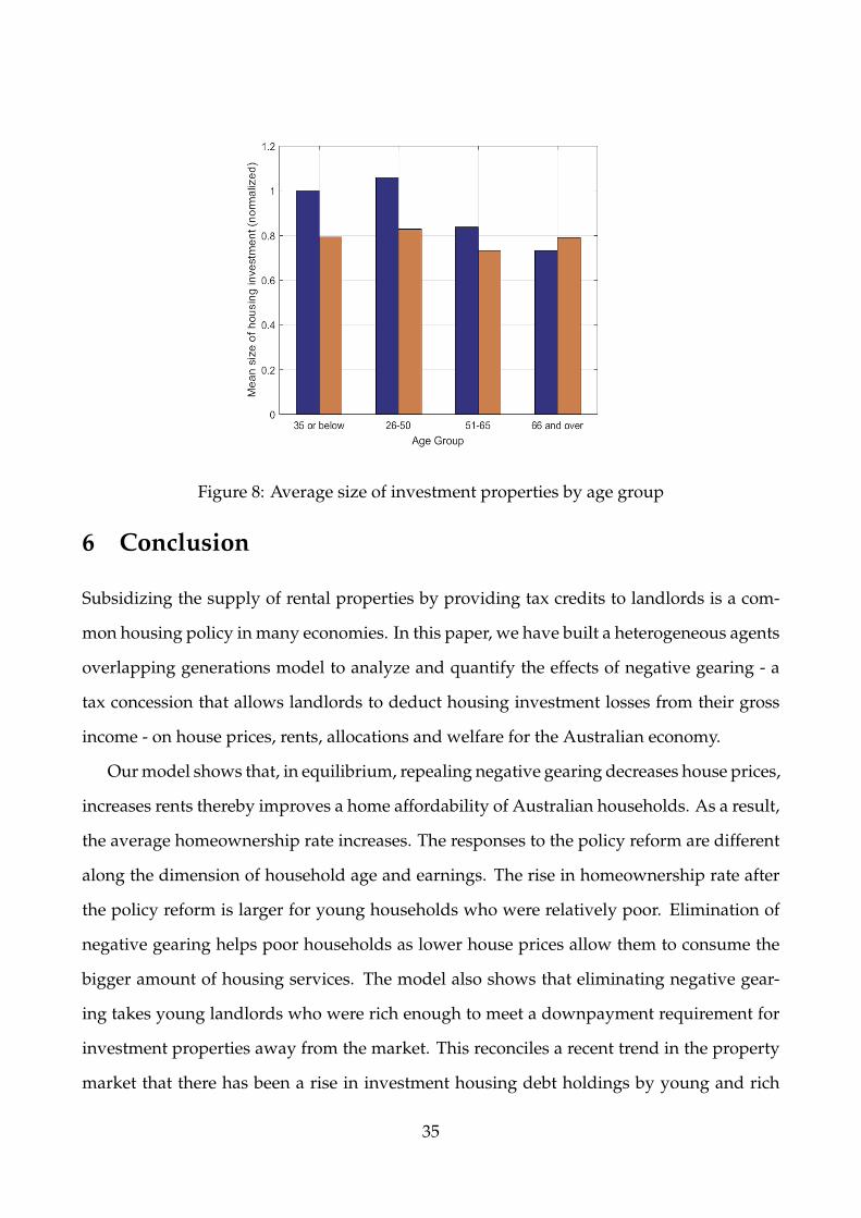
Figure 8: Average size of investment properties by age group

6 Conclusion

Subsidizing the supply of rental properties by providing tax credits to landlords is a com-

mon housing policy in many economies. In this paper, we have built a heterogeneous agents

overlapping generations model to analyze and quantify the effects of negative gearing - a

tax concession that allows landlords to deduct housing investment losses from their gross

income - on house prices, rents, allocations and welfare for the Australian economy.

Our model shows that, in equilibrium, repealing negative gearing decreases house prices,

increases rents thereby improves a home affordability of Australian households. As a result,

the average homeownership rate increases. The responses to the policy reform are different

along the dimension of household age and earnings. The rise in homeownership rate after

the policy reform is larger for young households who were relatively poor. Elimination of

negative gearing helps poor households as lower house prices allow them to consume the

bigger amount of housing services. The model also shows that eliminating negative gear-

ing takes young landlords who were rich enough to meet a downpayment requirement for

investment properties away from the market. This reconciles a recent trend in the property

market that there has been a rise in investment housing debt holdings by young and rich

35

households who would have benefited the most from negative gearing concessions.

The aggregate welfare for the economy improves upon the repeal of negative gearing.

Around 80 percent of households are better off after the policy reform. However, the welfare

effects on each household depends on their state at the time of the reform. Our analysis

suggests that the group of households hurt by the policy change is landlords who are young

and rich since most of them rely on mortgages to finance their housing investment. The

welfare loss for these landlords is exacerbated by the progressive tax system.

There are a number of extensions to this paper. First, the current model focus on a sta-

tionary equilibrium where ex-ante expected capital gains on housing asset is zero. Given the

recent boom in the Australian housing market, it is natural to embed a housing price appre-

ciation by changing the model structure to non-stationary with aggregate shocks to house

prices. Second, our paper only discusses the implications on eliminating negative gearing.

It would also be worth considering some partial restrictions on negative gearing such as

allowing tax deductions for mortgage interest payments only. Exploring implications of the

variation of negative gearing would be another policy scenario that is worth pursuing for

future research.

36

References

ALTONJI, J. G., AND L. M. SEGAL (1996): “Small-sample bias in GMM estimation of covari-

ance structures,” Journal of Business & Economic Statistics, 14(3), 353–366.

AUSTRALIAN TREASURY (2016): “Budget Paper 2016-17,” .

BERKOVEC, J., AND D. FULLERTON (1992): “A General Equilibrium Model of Housing,

Taxes, and Portfolio Choice,” Journal of Political Economy, 100(2), 390–429.

CHAMBERLAIN, G. (1984): “Panel data,” Handbook of econometrics, 2, 1247–1318.

CHAMBERS, M., C. GARRIGA, AND D. E. SCHLAGENHAUF (2009a): “Accounting for changes

in the homeownership rate,” International Economic Review, 50(3), 677–726.

CHAMBERS, M., C. GARRIGA, AND D. E. SCHLAGENHAUF (2009b): “Housing policy and

the progressivity of income taxation,” Journal of Monetary Economics, 56(8), 1116–1134.

CHATTERJEE, A., A. SINGH, AND T. STONE (2015): “Understanding wage inequality in Aus-

tralia,” The Economic Record, 92(298), 348–360.

CHATTERJEE, S., AND B. EYIGUNGOR (2015): “A quantitative analysis of the US housing and

mortgage markets and the foreclosure crisis,” Review of Economic Dynamics, 18(2), 165–184.

CONESA, J. C., S. KITAO, AND D. KRUEGER (2009): “Taxing capital? Not a bad idea after

all!,” The American economic review, 99(1), 25–48.

CORBAE, D., AND E. QUINTIN (2015): “Leverage and the foreclosure crisis,” Journal of Polit-

ical Economy, 123(1), 1–65.

FLODEN, M. (2008): “A note on the accuracy of Markov-chain approximations to highly

persistent AR (1) processes,” Economics Letters, 99(3), 516–520.

FLOETOTTO, M., M. KIRKER, AND J. STROEBEL (2016): “Government intervention in the

housing market: Who wins, who loses?,” Journal of Monetary Economics, 80(C), 106–123.

37

GERVAIS, M. (2002): “Housing taxation and capital accumulation,” Journal of Monetary Eco-

nomics, 49(7), 1461–1489.

GRATTAN INSTITUTE (2016): “Hot property: Negative gearing and capital gains tax reform,”

.

GUVENEN, F. (2009): “An empirical investigation of labor income processes,” Review of Eco-

nomic dynamics, 12(1), 58–79.

HEATHCOTE, J., K. STORESLETTEN, AND G. L. VIOLANTE (2014): “Consumption and labor

supply with partial insurance: An analytical framework,” The American Economic Review,

104(7), 2075–2126.

HONG, J. H., AND J.-V. RÍOS-RULL (2012): “Life insurance and household consumption,”

The American Economic Review, 102(7), 3701–3730.

JESKE, K., D. KRUEGER, AND K. MITMAN (2013): “Housing, mortgage bailout guarantees

and the macro economy,” Journal of Monetary Economics, 60(8), 917–935.

KAPLAN, G., K. MITMAN, AND G. VIOLANTE (2017): “The Housing Boom and Bust: Model

Meets Evidence,” Manuscript, University of Chicago.

LAIDLER, D. (1969): “Income tax incentives for owner-occupied housing,” The Taxation of

Income from Capital, pp. 50–76.

LIU, X., AND G. OTTO (2014): “Housing Supply Elasticity in Sydney Local Government

Areas,” Discussion paper, University of New South Wales.

NAKAJIMA, M. (2012): “Optimal capital income taxation with housing,” Discussion paper,

Federal Reserve Bank of Philadelphia.

POTERBA, J. M. (1984): “Tax subsidies to owner-occupied housing: an asset-market ap-

proach,” The Quarterly Journal of Economics, pp. 729–752.

38

(1992): “Taxation and housing: Old questions, new answers,” Discussion paper,

National Bureau of Economic Research.

ROSEN, H. S. (1985): “Housing subsidies: Effects on housing decisions, efficiency, and eq-

uity,” Handbook of Public Economics, 1, 375–420.

SOMMER, K., AND P. SULLIVAN (2016): “Implications of US tax policy for house prices,

rents and homeownership,” Discussion paper, Working Paper, Federal Reserve Board of

Governors.

STORESLETTEN, K., C. I. TELMER, AND A. YARON (2004): “Cyclical dynamics in idiosyn-

cratic labor market risk,” Journal of Political Economy, 112(3), 695–717.

TAUCHEN, G., AND R. HUSSEY (1991): “Quadrature-based methods for obtaining approxi-

mate solutions to nonlinear asset pricing models,” Econometrica, pp. 371–396.

39

Appendix

A0. Policy experiment without redistribution

In this section of appendix, we solve the model by shutting down the redistribution chan-

nel of government revenue created by eliminating negative gearing. Below, we provide the

steady state and welfare results by simulating the counterfactual economy with the same

level of transfer payments to the baseline economy. That is, the government uses the addi-

tional tax revenue for its own consumption which does not affect the decision of households.

Table 12: Steady state comparisons with and without redistibution

Baseline No NG (redist) No NG (no redist)Price 1.180 1.160 1.161Rent 0.164 0.168 0.168Price-rent ratio 7.209 6.907 6.911Frac. of homeowners 0.667 0.722 0.715Frac. of owner-occupiers 0.500 0.584 0.583Frac. of landlords 0.167 0.138 0.132Frac. of renters 0.333 0.278 0.285Rental supply (relative to housing supply) 0.263 0.184 0.178Aggregate housing supply (normalized) 1 0.987 0.987Transfers 0.229 0.236 0.229Debt to income ratio 0.356 0.304 0.305

The last column of Table 12 shows that the steady state moments of the counterfactual

economy without redistribution are very similar to that in the economy with redistribution.

The increase in lump-sum transfers hardly change the price and quantity effects of negative

gearing in steady states.

Turning to the welfare analysis, we find that there is a welfare loss when the government

does nothing with the additional revenue created by repealing negative gearing. The mean

of consumption equivalence variation, defined the same way as in the main body of the

paper, is -2.6 percent. Around 68 percent of households are worse off. The fall in house

prices hurts most homeowners especially elders who would be downsizing their dwellings.

40

Renters are worse off due to higher rents. Table 13 shows that the welfare loss is large for

landlords while it is smaller for renters and owner-occupiers. The lower homeownership

cost helps some renters (owner-occupiers) with housing purchase (upgrade) but the majority

of them prefer the status quo if there is no redistribution.

Tables 14 and 15 show the welfare effects by housing tenure across income quintiles

and age group. It is worth nothing that almost every landlord in the top income quintile

prefer the status quo while more than 50 percent of high income owner-occupiers marginally

prefer the counter-factual economy. Young owners-occupiers also prefer the counterfactual

economy since the lower house prices help them to climb up a housing ladder more easily.

Table 13: Welfare effects by housing tenure status

Initial Housing Tenure Mean CEV Median CEV Std. dev. CEV P(CEV > 0)Renter 0.007 -0.007 0.111 0.290Owner-occupier -0.053 -0.008 0.164 0.385Landlord -0.141 -0.057 0.251 0.265

Table 14: Welfare effects by housing tenure status and income quintiles

Median CEV P(CEV > 0)Initial Housing Income QuintileTenure Q1 Q2 Q3 Q4 Q5 Q1 Q2 Q3 Q4 Q5Renter -0.009 -0.004 -0.007 -0.016 -0.002 0.310 0.423 0.224 0.111 0.252Owner-occupier -0.020 -0.016 -0.010 0.001 0.006 0.268 0.267 0.280 0.519 0.642Landlord -0.024 -0.028 -0.064 -0.107 -0.346 0.169 0.298 0.308 0.203 0.036

Table 15: Welfare effects by housing tenure status and age group

Median CEV P(CEV > 0)Age Initial Housing Tenure StatusGroup Renter Owner-occupier Landlord Renter Owner-occupier LandlordUnder 35 -0.005 0.020 -0.123 0.308 0.753 0.28636− 50 -0.020 0.004 -0.128 0.264 0.551 0.27251− 65 -0.017 -0.011 -0.054 0.219 0.309 0.241Above 66 -0.009 -0.017 -0.004 0.317 0.233 0.487

41

A1. Estimation of Income Process

In this part of appendix, we provide the empirical estimates of income process using the

Australian household panel data – Household, Income and Labour Dynamics in Australia

(HILDA).

Data. The data are sourced from the HILDA, a longitudinal survey of Australian house-

holds which started in 2001. The HILDA survey is an ideal data set that enables us to inves-

tigate the dynamics of household income over the life-cycle, and to this date, 15 Waves are

available. The survey contains information of labor market activities, socio-economic and

demographic factors that are standard in a typical household survey. To begin with, we use

all observations in Waves from 1 to 15.

For the income variable we use the gross income reported at the individual level. In

HILDA, the gross income captures income sources from labor, business, investment, private

and public pensions, and government transfers. Since investment decisions are endogenous

in our model, we subtract the investment income component from the total gross income.

From this, we further trim the data set using the following criteria:

1. Male head of household;

2. Age between 21 and 64 years old;

3. Positive labor income;

4. Full-time workers; and

5. 10 consecutive years of appearance.

With the above restrictions, we end-up with the total of 1,514 individuals and 19,714 ob-

servations.

42

Model specification. The specification of labor income for individual i of age a is expressed

as:

log yi,a = γa + zi,a + εi,a

where γa is a deterministic component of income that depends on individuals’ age; zi,a is a

persistent idiosyncratic component; and εi,a is a transitory shock component of income. The

persistent idiosyncratic component follows an AR(1) process as below.

zi,a = ρzi,a−1 + ui,a ui,a ∼ (0, σ2u)

The above earnings process requires estimation of two components: (1) deterministic, γa

and (2) persistent and transitory shocks. The estimation of the deterministic component is

relatively straightforward. The deterministic component captures the income profile that

is common to all individuals in a particular age group, and also removes any predictable

patterns of the income process. To begin with, we consider a standard Mincerian regression

of the following form, run separately year-by-year.

log Yi,a,t = β′Xi,a,t + yiat (20)

where Yi,a,t is an annual gross income without any investment incomes. To remove any

predictable changes in earnings, we include the term Xi,a,t which captures observable de-

mographics such as age, education and race. The last term yi,a,t summarizes residuals of

the regressions. The deterministic component can then be traced out using the average log

income for each age group a and is fitted to a fourth-order polynomial function in age.

Residual process. We assume that the process is stationary. Although we obtain residuals

year-by-year, these residuals are averaged across years, i.e. yi,a ≡ yi,a,t. From this point

onwards, we drop the subscript t. Identification and estimation of nonstationary precess

are more complicated, see Heathcote, Storesletten, and Violante (2014) for example. The

43

Figure 9: Deterministic component

specification of the process of residual dispersion can then be written as

yi,a = zi,a + εi,a (21)

zi,a = ρzi,a−1 + ui,a (22)

where

εi,a ∼ IID(0, σ2ε ); ui,a ∼ IID(0, σ2

u); zi,0 ∼ IID(0, σ2z,0)

and

εi,a⊥ui,a⊥zi,0,

The parameters to be estimated are grouped into θ = ρ, σ2ε , σ2

u, σ2z,0.

Identification. We follow identification procedures discussed in Guvenen (2009) and

Storesletten, Telmer, and Yaron (2004). Identification in levels is based on the following

definitions of variances and covariances.

44

var(yi,0) = σz,0 + σε for a = 0

var(yi,a) = var(zi,a) + σε for a > 0

var(zi,a) = ρ2var(zi,a−1) + σu

cov(yi,a, yi,a−j) = cov(zi,a, zi,z−j) for j > 0

cov(zi,a, zi,a−j) = ρjvar(zi,a−j)

With these in hand, we can formulate the parameter identification as follows. First, the

AR(1) coefficient or the persistent parameter ρ is identified from the slope of the covariance

at lags.cov(yia, yi,a−2)

cov(yi,a−1, yi,a−2)=

ρ2var(zi,a−2)

ρvar(zi,a−2)= ρ

The variance of transitory component, σ2ε is identified from the difference between variance

and covariance

var(yi,a−1)− ρ−1cov(yia, yi,a−1) = var(ηi,a−1) + σε − var(ηi,a−1)

and the variance of initial persistent component, σ2z,0 can be obtained residually from σ2

ε and

var(yi, 0). Finally, the variance of error term in the AR(1) process, σ2u is identified from the

following.

var(yi,a−1)− cov(yia, yi,a−2)− σ2ε = ρ2var(ηi,a−2) + σ2

u + σ2ε − ρ2var(ηi,a−2)− σ2

ε

= σ2u

Therefore, the identification of parameters are achieved using two lags. In our case, the

model is largely identified since the HILDA survey is available for 15 waves. Also, the pa-

rameters are tightly estimated because the number of individuals in the panel is large. In

our baseline sample, there are 1,592 individuals.

45

Estimation. Our sample consists of the unbalanced panel of individuals aged a = 1, ..., A.

We define a A× 1 vector for every individual i = 1, ..., I.

di =

di,1

...

di,A

where di,a ∈ 0, 1 is an indicator variable for whether individual i is present at age a in the

sample. Similarly, define a A× 1 vector of residual earnings observations as

yi =

yi,1

...

yi,A

Since the panel is unbalanced, we must set the missing elements to zero. Now, let

Y =I

∑i=1

yiy′i D =I

∑i=1

did′i

The covariance of earnings is then a A× A symmetric matrix, C, computed as the element

by element division between Y and D

C =YD

The construction of covariance matrix C is as follows:

46

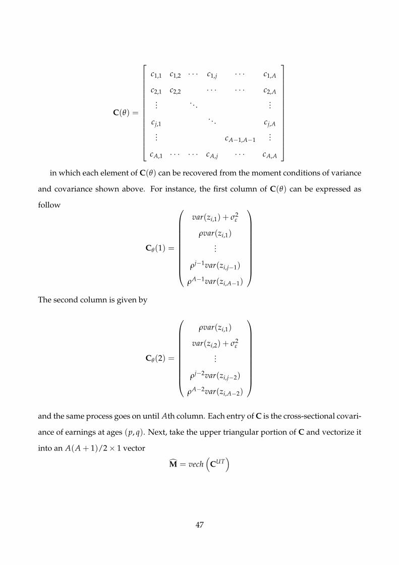
C(θ) =

c1,1 c1,2 · · · c1,j · · · c1,A

c2,1 c2,2 · · · · · · c2,A... . . . ...

cj,1. . . cj,A

... cA−1,A−1...

cA,1 · · · · · · cA,j · · · cA,A

in which each element of C(θ) can be recovered from the moment conditions of variance

and covariance shown above. For instance, the first column of C(θ) can be expressed as

follow

Cθ(1) =

var(zi,1) + σ2ε

ρvar(zi,1)

...

ρj−1var(zi,j−1)

ρA−1var(zi,A−1)

The second column is given by

Cθ(2) =

ρvar(zi,1)

var(zi,2) + σ2ε

...

ρj−2var(zi,j−2)

ρA−2var(zi,A−2)

and the same process goes on until Ath column. Each entry of C is the cross-sectional covari-

ance of earnings at ages (p, q). Next, take the upper triangular portion of C and vectorize it

into an A(A + 1)/2× 1 vector

M = vech(

CUT)

47

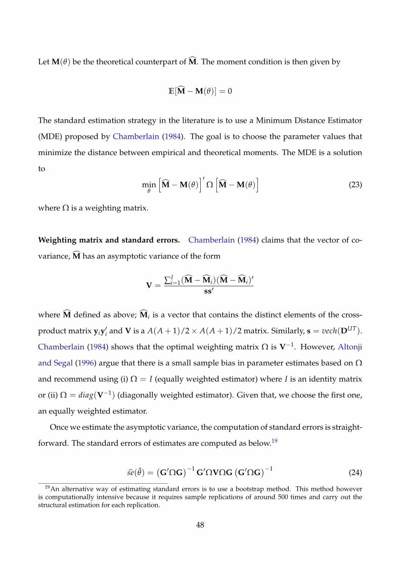
Let M(θ) be the theoretical counterpart of M. The moment condition is then given by

E[M−M(θ)] = 0

The standard estimation strategy in the literature is to use a Minimum Distance Estimator

(MDE) proposed by Chamberlain (1984). The goal is to choose the parameter values that

minimize the distance between empirical and theoretical moments. The MDE is a solution

to

minθ

[M−M(θ)

]′Ω[M−M(θ)

](23)

where Ω is a weighting matrix.

Weighting matrix and standard errors. Chamberlain (1984) claims that the vector of co-

variance, M has an asymptotic variance of the form

V =∑I

i=1(M− Mi)(M− Mi)′

ss′

where M defined as above; Mi is a vector that contains the distinct elements of the cross-

product matrix yiy′i and V is a A(A + 1)/2× A(A + 1)/2 matrix. Similarly, s = vech(DUT).

Chamberlain (1984) shows that the optimal weighting matrix Ω is V−1. However, Altonji

and Segal (1996) argue that there is a small sample bias in parameter estimates based on Ω

and recommend using (i) Ω = I (equally weighted estimator) where I is an identity matrix

or (ii) Ω = diag(V−1) (diagonally weighted estimator). Given that, we choose the first one,

an equally weighted estimator.

Once we estimate the asymptotic variance, the computation of standard errors is straight-

forward. The standard errors of estimates are computed as below.19

se(θ) =(G′ΩG

)−1 G′ΩVΩG(G′ΩG

)−1 (24)

19An alternative way of estimating standard errors is to use a bootstrap method. This method howeveris computationally intensive because it requires sample replications of around 500 times and carry out thestructural estimation for each replication.

48

Table 16: Estimates of income process using HILDA

10 consecutive 5 consecutiveρ 0.9407 0.9557

(0.0078) (0.0061)σ2

u 0.0302 0.0259(0.0001) (0.0000)

σ2z,0 0.1376 0.1678

(0.0003) (0.0000)σ2

ε 0.0805 0.1405(0.0026) (0.0052)

No. of individuals 1541 3341Note: The model is estimated using the minimum dis-tance method. Asymptotic standard errors are reportedin parentheses.

where G is the A(A + 1)/2× n Jacobian matrix of M(θ) evaluated at the estimated param-

eter values. The letter n represents the number of estimated parameters in our statistical

model.

Result. In the second column of Table 16, we report the results using the baseline sam-

ple. The persistent component, ρ is slightly lower than a random walk process. The results

also suggest that the variance of transitory component is higher than that of the persistent

component, consistent with the findings by Chatterjee, Singh, and Stone (2015). We also pro-

vide in the last column of Table 16 the results based on 5 consecutive years of appearance.

When we relax such a restriction on the consecutive years of appearance, we observe slightly

higher persistence and lower variances of both persistent and transitory components.

Simulation. Since the HILDA survey is available for only 15 years, it lacks the sufficient

time lags to estimate parameters of interest, especially when we need to calibrate our model

in which one period accounts for five years.20 Here, we introduce a simulation technique

that enables us to approximate earnings process parameters with any model periods.

20Although the re-interview rate in HILDA is reasonably high, only a few households remain in the surveyfor the entire 15 years of the survey period.

49

We follow the procedure below to obtain the panel of model implied income. This simu-

lation provides us with a distribution of income that has both cross-sectional and time-series

properties implied by the annual parameter estimates.

1. Draw an initial sample of 5,000 individuals, entering the model economy at the age of

21. Also we assume that zi,0 = 0

2. For each individual and period:

(a) Draw a death shock. This shock comes from the binomial distribution where the

survival probabilities are obtained from the Life Table published by the ABS.

(b) If survive, continue with the income process specified above.

(c) If die, replace this individual with a new individual entering the model with age

21. The new individual starts her life-cycle from this period, as noted in (a) and

(b).

3. Continue this process for 120 periods. It gives us the unbalanced panel consists of

600,000 observations and 20,521 individuals exiting the panel at different ages.

After obtaining the large panel of income data, we perform the MDE for each model

period. For brevity, we provide the estimates for 2, 3, 4, and 5 years. These estimates provide

a useful source for income process calibrations in our income process. The simulated data

can also be used to estimate income process parameters for any period. The results are

reported in Table 17. The estimates for the AR(1) coefficient become lower as the number of

model period increases. In contrast, the variance of idiosyncratic component, σ2u, increases as

the number of model period increases. These observations make intuitive sense as earnings

are less persistent (lower ρ) and more volatile (higher σ2u) for longer periods. It thus suggests

that the mean reversion becomes increasingly a more important determinant in earnings

dynamics as we increase the number of periods, and that a random walk specification is not

sufficient to understand the income process for models with longer time horizons. We also

provide the annual estimates using the simulated data. Encouragingly, the key parameters,

50

Table 17: Estimates of income process using simulated data

Actual 1 year 2 year 3 year 4 year 5 yearρ 0.9407 0.9200 0.8367 0.7675 0.7261 0.6404

(0.0078) (0.0001) (0.0035) (0.0006) (0.0003) (0.0003)σ2

u 0.0302 0.0434 0.1030 0.1525 0.1948 0.2357(0.0001) (0.0001) (0.0006) (0.0015) (0.0028) (0.0057)

σ2z,0 0.1376 0.2185 0.1775 0.1337 0.0640 5.1 ×10−7

(0.0003) (0.0004) (0.0023) (0.0058) (0.0094) (0.0022)σ2

ε 0.0805 0.0369 9.9 ×10−9 6.8 ×10−7 1.3×10−9 0.0041(0.0026) (0.0015) (0.0034) (0.0060) (0.0096) (0.0137)

No. of individuals 1,541 18,566 18,283 17,623 16,570 15,048Note: The data are generated from simulation. The model is estimated using the minimum dis-tance method. Asymptotic standard errors are reported in parentheses.

ρ and σ2u are close to the actual estimates reported in Table 1, reinforcing the credibility of

our simulation procedure.

We also run an additional simulation to support that the above simulation is sufficient

to generate a panel that is a good representation of the actual data.21 To briefly explain the

procedure, for every period (after the step 2 above), we count the number of individuals for

each age cohort and calculate the average income across all individuals. We then simulate

the economy until the distribution of individuals across age cohorts and the average income

are not changing over time. In this way, the stationary distribution is achieved in 55 peri-

ods. This additional exercise supports the idea that the panel we obtained has an unbiased

representation of population.

A2. Computational details

Computation of Stationary Equilibria

State space, choice variable, and timing of event. A household’s current state is deter-

mined by four individual vectors, savings s, the housing asset h−1, the realization of income

shock z, and age a. The choice variables include savings s′, housing asset h, housing ser-

21We run this simulation using the 5 year estimates, but the estimates from any model periods to verify this.

51

vices h, and non-durable consumption c. The risk-free asset is discretized into 60 spaces.

Households are allowed to choose the maximum possible borrowing for each housing size,

s = (1 − θ)ph. We define this as knots. Between each pair of knots, we allow for three

equally spaced grids so that it gives more flexibility in choosing the size of mortgages. The

saving grid is more finely spaced for lower levels of borrowings. For positive s, we use the

increment of $10,000 for savings up to $200,000, and $50,000 up to the maximum value which

is capped at $1,000,000. Houses are available in K = 9 discrete sizes, h ∈ 0, h(1), ..., h(9).

Increasing the number for K increases the computational speed exponentially. The smallest

housing size, h(1) is set at 80 percent of the median income corresponding to the actual value

of $278, 700. So in the baseline, the value of smallest house is $328,866. We cap the largest

housing size at the actual value of $1,500,000. Houses available to renters can be smaller

than the minimum housing size, we include three extra housing sizes for rent below h(1)

such that hrent ∈ hrent(1), .., hrent(3), h(1), ..., h(9). This is the grid for housing services for

renters. The state space for idiosycratic income shocks is discretized into five states using

the method of Tauchen and Hussey (1991).

It would be useful to describe the timing of event within a period. In any period of life,

households face the following events sequentially:

1. Endowments are realized

– idiosyncratic income shocks determine labor income

– savings from the previous period provide return. If borrowed, households need

to pay mortgage interest

2. Housing and asset decisions are made

– sell (1− δ)h−1 and choose h

– altering the net level of housing stocks, i.e. h−1 6= h incurs transaction costs

Housing consumption is given by

52

– if h ≥ h > 0, the household consumes housing services from owner-occupied

housing stocks

– if h > h = 0, the household consumes housing services by renting a house

If h > h > 0, then the household becomes a landlord and receive a rental yield of NRI,

defined as (6).

3. Pay tax levied on taxable income, given by (7) for the baseline economy. Receive the

lump-sum transfer F.

4. Choose non-durable consumption c and finalize the amount of savings and borrow-

ings s′.

Computation of stationary equilibrium. The stationary equilibrium is computed using

constant prices, rents and transfers. We start first by guessing a those three equilibrium ob-

jects. Given prices, rents and transfers, we compute the optimal policy and value functions

for the last period, A = 14. We then solve the household problem for all other periods using

backward induction. Once we obtain policy functions, we simulate forward the economy

until a stationary distribution of households over the state space is achieved. In doing so,

we draw 100,000 households. Each household start their life-cycle with zero savings and

housing stocks. After the end of each period, households receive an age-dependent death

shock in which the death rate is obtained from the Life Table (2007-08 release) published by

the ABS. We assume that the death shock follows the binomial distribution. Households

exit the economy with certainty after 14 periods. If a household survives, he continues to

make choices, and we simulate the optimal behavior of these households forward using the

policy functions. If a household dies, he is replaced by a newly born household who starts

his life-cycle from the following period. The stationary distribution is obtained when the

cohort distribution and the mean of savings do not change over time. Finally, we iterate the

whole process until the market clearing price, rent, and the lump-sum transfer that gives

the balanced budget for the government are found. We provide more details on this in the

53

following section.

Finding market clearing prices and rents. We follow an algorithm provided in Sommer

and Sullivan (2016) in finding market clearing prices and rents. In a simulated economy,

there is a cross-section of N = 100, 000 households. The market clearing condition for hous-

ing and rental markets are given by

N

∑i=1

hi(p∗, pr∗|z) = H

N

∑i=1

hi(p∗, pr∗|z) = H

Solving for the equilibrium of the housing and rental markets is very time consuming be-

cause it involves repeatedly solving the household dynamic programming at potential equi-

librium prices and simulating data to check for market clearing until the equilibrium prices

are found.

Let pk and prk be the kth guess of the market clearing house price and rent, and let pr

k(pk)

represent the rent that clears the market for housing conditional on house price pk. Now

consider the following excess demand functions

EDhk (pk, pr

k) =N

∑i=1

hi(p∗, pr∗|z)− H

EDhk (pk, pr

k) =N

∑i=1

hi(p∗, pr∗|z)− H

The equilibrium house price p∗ and rent pr∗ simultaneously clear the housing and rental

market such that

EDhk (pk, pr

k) = 0

EDhk (pk, pr

k) = 0

54

Algorithm:

1. Make an initial guess of the market clearing house rent prk.

2. Search for the rent prk(pk) which gives EDk(pk, pr

k) = 0, conditional on the fixed house

price. This step requires re-solving the household problem at each trial value of prk(pk),

simulating data using the optimal policy functions and checking for market clearing

in the simulated data.

The bisection method is used to find the equilibrium rent.

3. Once the set of price and rent (pk, prk(pk)) that clears the housing market is found,

check also if this pair clears the rental market by evaluating Dhk (pk, pr

k) = 0

a) if EDhk (pk, pr

k) < 0 and k = 1, the initial guess p1 is too high, so set pk+1 = pk − ε

and go to Step 2.

b) if EDhk (pk, pr

k) > 0 and k = 1, the initial guess p1 is too low, so set pk+1 = pk + ε

and go to Step 2.

c) if EDhk (pk, pr

k) > 0, the equilibrium prices are found, so stop.

55