negotiated red zones around hazardous plants
TRANSCRIPT

Negotiated Red Zones Around Hazardous Plants∗
Céline Grislain-Letrémy† Bertrand Villeneuve‡
January 5, 2016
Abstract
This paper studies the negotiations of red zones in urban areas exposed to industrial disasters. Wecompare typical scenarios regarding the distribution of bargaining power between the firm and thecity. We explain how red zones are revised as technology, climate, or demography change, and weshow how and why responses are neatly distinct across scenarios. Further, we give and explain theconditions for industrial sanctuaries (as the population grows) and city cores (as the risk grows).
Keywords: industrial disasters, land-use regulation, land-use negotiation, climate change.
JEL classification: R52, Q53, Q54, Q56.
∗This paper was originally part of a paper which circulated under the title “Natural and Industrial Disasters: LandUse and Insurance.” It has benefited from comments by participants at the CREST internal seminars, the UniversityParis-Dauphine research day, the ETH Zurich and University of Nantes seminars, the Symposium on France-TaiwanFrontiers of Science and the World Risk and Insurance Economics Congress. This study was supported the Financeand Sustainable Development Chair (Institut Europlace de Finance) and the Fondation du Risque. The authors thankNicolas Grislain, Frédéric Loss, and Marion Oury for their comments. They also thank Valérie Sanseverino-Godfrinfor explanations about law and legal precedents, and Cédric Peinturier and Clément Lenoble for explanations aboutrisk engineering.†CREST and Université Paris-Dauphine, PSL Research University. Email: [email protected]‡Université Paris-Dauphine, PSL Research University, and CREST. Email: [email protected]

1 Introduction
The urbanization in the vicinity of industrial plants increases the magnitude of industrial disasters.The gas leak from the Union Carbide India Limited pesticide plant in Bhopal in 1984 is dramaticevidence of this trend (Ferrante, 2011). As is the explosion of the AZF plant in Toulouse (France)in 2001.1 The number of deaths and casualties due to a fertilizer plant explosion in North Texas inApril 2013 is also attributable to the urbanization in the neighborhood around the plant.2 Overall,the economic costs of industrial disasters has risen dramatically over the last few decades (Figure4, page 6 in Bevere et al., 2015).
The firm that causes the damages is liable for them. Indeed, even though the intertwinedhistories of risk and urban development can be complex, the law is quite simple: there is no rightof “initial land use” by which the industrialist can renege on its responsibility for any disastercompensation to the newcomers. Consequently, households and businesses do not have to pay forthe risk they create by locating in exposed areas. In particular, they do not need to purchaseinsurance against these risks, except perhaps legal assistance insurance. This protection mightexplain why households and businesses can exist in proximity to hazardous areas. Other plausiblereasons could be ignorance, perception biases, or employment by hazardous facilities. We proposehere a basic and pure analysis of the negative externality that the “curse of unlimited liability”implies: fully compensated households occupy the available land and, in doing so, they increase thecost of compensation for the firm in the case of a disaster. The limited liability of the firm cancertainly produce interesting effects: excessive risk-taking by the firm and, in turn, more prudentlocation choices by imperfectly protected households.3 We consider the non-life losses from industrialdisasters. Presumably, if households take into account irreplaceable assets, such as health, theyshould make less risky location choices.
To contain their liabilities, the industrialists can purchase or rent land, establishing an exclusionzone, also called a red zone, which is the focus of our analysis. For example, in Louisiana, the DowChemical company in 1991 paid for a whole village of 300 inhabitants to move out of the vicinity ofone of its chemical plants (Sauvage, 1997). Or the state can delimit red zones. European memberstates design land use policies such that appropriate distances are maintained between hazardousfacilities and residential areas.4 In practice, the firm can decide to rent the land or the state or
1The AZF website illustrates how the Toulouse agglomeration progressively has encircled the plant. See link.2M. Fernandez and S. Greenhouse, “Texas Fertilizer Plant Fell Through Regulatory Cracks.” New York Times
April 24, 2013 (link). The New York Times’ website provides a map of the plant and its vicinity (link).3Several empirical works that use the hedonic prices method show that the perception of industrial risks can
decrease property values to an extent that depends on information release (Boxall et al., 2005; Kiel and McClain,1995; McMillen and Thorsnes, 2003) and that varies among sites (Gawande and Jenkins-Smith, 2001; Grislain-Letrémyand Katossky, 2014; Kiel and Williams, 2007).
4See Article 12 on the Control of Urbanization in the Council Directive 96/82/EC of 9 December 1996 on thecontrol of major accident hazards involving dangerous substances. See Basta (2009) for a comparison of implementedred zones around hazardous plants between European countries.
1

a city can encourage renting (Sauvage, 1997). Red zones result from a negotiation between thehouseholds (e.g. through the mayor) and the firm, because extending the region where building isforbidden reduces the total cost of risk but crowds households at the same time.
This paper analyzes red zones as a strategy to reduce the costs of industrial disasters. In oursetting, the firm does not need land per se; it only wants to prevent potential victims from occupyingthe riskiest locations. We develop an urban model of a linear city with a significant risk gradient.A possible picture is that of a new developing region with a hazardous plant on one side and onthe other, for example, a mountain or an already saturated area. We derive our model from theclassical urban economics literature (see Fujita and Thisse, 2002, for a review). For the sake ofsimplicity, we assume that the firm does not employ any of the households in our area: their lossesare only material and direct.
This paper proposes a positive analysis on the negotiation of red zones. The normative side isclear: these commonly used red zones are optimal as long as potential losses are proportional tothe surface used. We focus the analysis on the mechanisms through which the bargaining power ofthe industrialist impacts the design of red zones and their evolution with respect to technologicaland climatic changes and demographic evolution. The literature studies the maneuvers by firms topurchase land but not from the angle of risk exposure. Our analysis fills this gap in the study ofindustrial risks. The analysis of takeover bids as in Grossman and Hart (1980) is a valid sourceof inspiration for solutions. Blume et al. (1984) and Nosal (2001) study the efficiency of payingcompensation; Miceli and Segerson (2006) and Strange (1995) analyze the problem of the holdup adeveloper faces when individual landowners know that their parcel of land is necessary for projectcompletion and can postpone or even block the overall project.
We show that the stronger the bargaining power of the industrialist, the larger the red zone.We study the four patterns in typical real estate markets: bargaining power lying with the firm orwith the mayor (acting in the interests of the citizens), price-taking behaviors on both sides, andthe extreme case where the firm is entirely the property of the households. The last scenario is theworst case for households, because they bear the entire cost of risk; this is why it corresponds tothe largest red zone.
We determine the impact of risk changes and the population evolution in red zones. Theincreasing cost of industrial disasters is largely explained by the growing urbanization of risky areas.Industrial hazards can also change because of technological progress, reassessed risk, and climatechange, because they might be linked to evolving natural hazards. An increase in risk should causean extension of the red zone, whereas an increase in population should cause a reduction in thered zone. We show that the variations in the red zone depend on the game played, even for givenfundamental parameters like household preferences. An increase in risk expands the red zone in thescenarios where the agents who pay the cost of risk control the red zone. In the other scenarios,
2

the variations can be reversed. But the scenario does not alone explain the variations in the sizeof the red zone: the same scenario can lead to an increasing red zone with some preferences and adecreasing red zone with other preferences.
Such a variety of possibilities for the net impact calls for a clarification of the mechanisms thatdetermine the red zones. There are two opposite impacts at the origin of the ambiguity. On the onehand, an increase in risk or in population raises the cost of risk. On the other hand, the demandfor land increases as the population increases. A third, and more complex, effect is at play: thekey factor is the variation in the households’ willingness to pay for space as their wealth increases.If rents increase (e.g., because the rise in the cost of risk leads the firm to bid higher rents), thenhouseholds pay and receive higher rents. The net impact can go both ways, as we show. Werigorously define and discuss these three effects in detail in the general case, and we illustrate themas well as the net impact with parametric calculable examples.
This paper proceeds as follows: Section 2 sets up the model. Section 3 compares the optimal redzones for the different scenarios of bargaining power between the households and the firm. Section4 details the impact of technological or climate change and demographic evolution on the size ofthe red zones. Section 5 concludes.
2 Model
2.1 Space and risk
City. We model a city with a risk gradient. The interval [0; x] is the linear space of inhabitablelocations. The hazardous plant is located at 0. The distance x to the source determines the riskexposure at a given location. The safest place x can be seen as an outer limit of the territory(Figure 1). The cost of living somewhere comprises the cost of risk and transportation costs. In thetradition of urban economics models, the latter would be related to the distance to the center. Sincetransportation costs are well understood, we neglect them in this study to keep the tractability ofthe model. The total population is N .
Risk. Location x will be damaged only once with probability p(x) with
∀x, p(x) := ρ f(x), (1)
where function f(·) is positive, decreasing along the space line, and piecewise continuous; and ρ > 0is a magnitude index for comparative statics. The damage per dwelling of size s is λF + λS s; thefirst part λF ≥ 0 is fixed and the other part is λS s with λS ≥ 0 and is proportional to the house’ssize. The damage corresponds to the (re)building cost and does not depend on the land’s value.
3

There is no damage to empty places. The expected damage for a dwelling of size s at location x is
p(x) (λF + λS s). (2)
This specification captures the essential facts. The risks can be correlated across locations. If anexplosion or contamination reaches location x, then it also reaches location x′ with 0 < x′ < x.This correlation gives the simplest justification for assuming that the function p(·) decreases. Overthe time period considered, p(x) is also the expected number of events, rather than the probabilityof a single event.
Coverage. All households are de facto insured by the industrialist. Because the firm is liable forall damages, there is no need for households to take out insurance. We assume that after a disasterthe industrialist provides complete reimbursement λF + λS s. We assume that the firm itself isrisk-neutral or equivalently that risk-neutral insurers fully insure the firm.
Red zone. We define the red zone as the area rented by the firm. The firm does not need landper se; it only wants to prevent potential victims from occupying the riskiest locations. In the otherzone, land use by households is not restricted. The location x∗ denotes both the size of the red zoneand the leftmost inhabited location (Figure 1).
Building zoneRed zone
Hazardous plant
Safest location
Figure 1: Space and risk.
Land occupation. A household lives at a given location x in [0; x]; its dwelling occupies lotsize s(x) and the density of the households at location x is n(x). Because households are fullycovered, all of the permitted locations have the same value, and the building zone [x∗, x] is fullyand uniformly used. Therefore:s(x) = x−x∗
N = 1n(x) if x ∈ [x∗, x],
s(x) = 0 and n(x) = 0 otherwise.(SUR)
Rent. The rent r is the price per unit of a lot size at x. The rent is uniform, as is the occupation,in the authorized area [x∗, x]. Further, the households have equal shares in a fund that owns all ofthe land. Any reforms have an identical effect on each household. This effect is the implementation,
4
by a fair-minded mayor, of compensation when the city enacts a zoning law, so that there are neverlosers and winners at the same time. The households each receive an additional income r that theytake as given:
r := x− x∗
Nr. (3)
Cost of risk. With uniform land-use over the inhabited area [x∗, x], the total expected cost ofthe risk (CR) amounts to
CR(x∗) :=∫ x
x∗p(t) (λF + λSs(t)) n(t) dt, (4)
=(
N
x− x∗λF + λS
)×∫ x
x∗p(t) dt. (5)
Increasing x∗ decreases the cost of risk, therefore increasing x∗ leads to a positive marginal riskreduction (MRR).
MRR(x∗) := −dCRdx≥ 0. (6)
We assume that the marginal benefit of reducing the cost of the risk decreases. In other words, weassume that
CR(·) is convex. (CVX)
A convex p(·) is a sufficient condition to get a convex CR(·).
The red zones partially correct the imperfect internalization of risk and can increase efficiency.The red zone is the only variable that the firm or policy can change to reach an optimum: increas-ing x∗ reduces the cost of risk and the available space at the same time. The firm compensateshouseholds for being squeezed by an amount denoted by T , each of them receive T/N before theysettle in.
2.2 Households
Households are identical and have no intrinsic preference for one location over another. Their utilityU(z, s) depends on their consumption z of the composite good (henceforth money) and on theirhousing size s. The function U is twice differentiable and strictly increases with respect to z > 0and s > 0. Indifference curves are strictly convex and do not cut axes.5
Households are price takers; they have an income ω, and they maximize their expected utilityunder their budget constraint. Because coverage is complete, the expected utility EU is no morethan the utility U . Households’ (HH) choice (x, z, s) solves
maxx,z,s
U(z, s) s.t. ω + �r + T
N≥ z +��sr and x ∈ [x∗, x], (HH)
5Similar to Assumption 2.1 in Fujita (1989).
5

where r = sr as shown by Equations (SUR) and (3).
We denote MRSsz the marginal rate of substitution of s for z, that is,
MRSsz := ∂U/∂s
∂U/∂z. (7)
MRSzs is simply the reciprocal. We assume that the Engel curves increase:
∀(z, s), ∂MRSzs∂z = ∂
∂z
(∂U/∂z∂U/∂s
)≤ 0,
∀(z, s), ∂MRSsz∂s = ∂
∂s
(∂U/∂s∂U/∂z
)≤ 0.
(ENG)
These two assumptions indicate that the relative value of the commodity that is becoming moreabundant decreases; they are ordinal sufficient conditions for increasing Engel curves.
2.3 Optimality
A red zone policy is said to be constrained optimal if it is Pareto optimal under the followingconstraints: (i) physical constraint (SUR) and (ii) no household envies another household.
The constrained-optimal allocations can be parametrized by (T ∗, x∗), where T ∗ is the net transferfrom the firm to households. They are characterized by programs where the utility of the householdsis maximized given a minimum profit for the firm of Π:
max(T,x)
U(ω + T
N ,x−xN
),
s.t. π − T − CR(x) ≥ Π,0 ≤ x ≤ x.
(8)
where π is the unmodeled profit generated by the firm’s primary activity. This unmodeled profitcould depend on T , if the transfer impacts the marginal cost of capital; or x, if land has some use.In such an extension, the firm would not simply try to reduce risk but would preserve profits minusthe cost of risk. In a sense, the cost of risk could be redefined to integrate several economic effects.
3 Bargaining scenarios
The size of the red zone results from a negotiation between the firm and the mayor. The fact thathouseholds are landowners makes them likely to benefit from the firm renting their land, but thedistribution of the benefits of risk reduction depends on the market’s organization.
We study three typical patterns in real estate markets that correspond to different distributionsof bargaining power between the firm and the mayor. In these three cases, households are neitheremployees, owners of the firm, nor consumers of its production. We complete the scope with afourth and extreme opposite case where the firm is entirely the property of the households.
6

Dominant mayor scenario. In this scenario, the mayor holds the bargaining power and redis-tributes to households the benefits of the risk reduction extracted from the firm.
1. The mayor offers two different rents: one for households and one for the firm. The mayoralso requires a lump-sum transfer from the firm to be redistributed to the households.
2. The firm accepts or declines the offer. The firm’s reference for acceptance is the absenceof a red zone.
3. The households make their location choices.
Market scenario. The surplus is partly captured by the firm via access to the land and partlyrecovered by households via rents. The households and the firm are both price takers andmake their choices simultaneously. The equilibrium in the land market determines the redzone.
Dominant firm scenario. In this scenario, the firm holds the bargaining power and captures allthe surplus generated by the transaction.
1. The firm offers a two-part tariff: it chooses the rent per unit of land and the lump-sumtransfer to the community.
2. The mayor accepts or declines the offer. Acceptance by the mayor depends on householdsdoing at least as well as without the red zone.
3. The households make their location choices.
Integrated scenario. The firm is entirely the property of the households, who decide the size ofthe red zone.
1. The mayor decides the size of the red zone.
2. The households make their location choices.
The two different rents (in the dominant mayor scenario) or the two-part tariff (in the dominantfirm scenario) allow efficient extraction of the surplus by the dominant player.
An equilibrium allocation is generically denoted by (T ∗i , x∗i ), where i indicates the relevantscenario (i ∈ {Mayor, Market, Firm, Integ}).
Proposition 1. In the four scenarios, the equilibrium allocation (T ∗i , x∗i ) exists and is constrainedoptimal; for the dominant mayor, dominant firm, and the integrated scenarios, the equilibriumallocation is unique.
Proof. See Appendix A.1.
7

We can order the sizes of the four red zones. Proposition 1 implies that the equilibrium alloca-tions are all located on the constrained Pareto frontier. Households and the firm rank scenarios inopposite orders because an increase in T ∗ benefits the households but hurts the firm, whereas anincrease in x∗ benefits the firm but hurts the households. Comparing the transfers from the firm tothe households between the scenarios amounts to comparing the bargaining position of the mayorin each scenario. First comes the dominant mayor scenario, and then comes the market scenarioand the dominant firm scenario. The integrated scenario is the worst case for households becausethey bear the entire cost of risk. Thus:
T ∗Mayor ≥ T ∗Market ≥ T ∗Firm ≥ T ∗Integ. (9)
Proposition 2 compares the red zones and shows that households have more space when theirbargaining power is more favorable.
Proposition 2. We order the four red zones as follows:
x∗Mayor ≤ x∗Market ≤ x∗Firm ≤ x∗Integ. (10)
Proof. From (8), ( 1N
∂MRSsz∂s
+ dMRRdx
)dx∗
dTi= 1N
(∂MRSsz∂z
). (11)
The conditions (CVX) and (ENG) are sufficient for the red zone x∗ to decrease with respect to Ti.Using (9), we can readily order the sizes of the four red zones.
4 Evolution of red zones
For given fundamentals, the red zone depends on the bargaining game played. We explore thisresult further by showing how different societies digest new data. In other terms, we propose acomparative study of the scenarios when the parameters change.6
4.1 Causes of change
The conditions surrounding a given community are likely to change. The number of people andbusinesses located in the exposed areas and the value of their assets strongly determine the economiccost of industrial disasters (Bevere et al., 2011). Technological improvements or, contrariwise,negligence and deterioration of structures happen continually.
6Our approach is similar to Pines and Sadka (1986), who establish comparative statics of an empty zone in acity inside which transportation costs vary (but not risk exposure). They show that the empty space can increase ordecrease with respect to population size.
8

Climate change is also a relevant factor to be regularly reassessed, because it is likely to increasethe intensity and the frequency of natural hazards (Schneider et al., 2007). Indeed, natural andindustrial hazards can also mutually aggravate each other. For example, the increase of landslidesand seismic activity due to the Three Gorges Dam in China is now officially recognized by Chineseauthorities.7 Similarly, hydraulic fracturing causes earthquakes of a very low intensity and mightalso cause moderate earthquakes.8
4.2 A decomposition in basic effects
Reasonably, an increase in risk should cause an extension of the red zone, whereas an increase inpopulation should cause a reduction in the red zone. This reasoning would be true if there was asingle decision maker. In fact, an increase in risk leads the firm to bid higher rents to extend thered zone. This increase in rent has a substitution effect on households (because they pay rents asrenters) and an income effect (because they receive rents as landowners). The net impact dependson the elasticity of substitution between land and money. The intricacy of effects calls for theirsystematic separation and quantification and for their illustration by calculable applications.
Three effects can be distinguished as: (1) the risk intensification effect that increases the firm’swillingness to extend the red zone, (2) the income effect caused by the change in the households’share of wealth and the risk that modifies their bid for land, and (3) in the case of the changesin population size, the land sharing effect, that is the mechanical increase in the marginal bid forland due to demographic expansion. These three effects are mathematically defined in AppendixA.2. The changes in ρ summarize climate change, and the changes in N summarize demographicevolution.
Proposition 3. Under assumptions (CVX) on risk and (ENG) on preferences,
1. The sign of dx∗/dρ is the sign of
Risk intensification effect of ρ + Income effect of ρ.
The land sharing effect is null.
2. The sign of dx∗/dN is the sign of
Risk intensification effect of N + Income effect of N + Land sharing effect of N .7M. Hvistendahl, “China’s Three Gorges Dam: An Environmental Catastrophe?” Scientific American March 25,
2008. See link.8Seismologists at Columbia University consider that earthquakes that hit Youngstown (Ohio) in 2011 (including
a 4.0 magnitude earthquake) are probably linked to the disposal of the wastewater from hydraulic fracturing. SeeLamont-Doherty Earth Observatory, “Ohio Quakes Probably Triggered by Waste Disposal Well, Say Seismologists”(Press release, January 6, 2012). Cf. link.
9
Proof. See Appendix A.2.
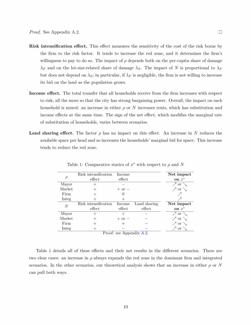
Risk intensification effect. This effect measures the sensitivity of the cost of the risk borne bythe firm to the risk factor. It tends to increase the red zone, and it determines the firm’swillingness to pay to do so. The impact of ρ depends both on the per-capita share of damageλF and on the lot-size-related share of damage λS . The impact of N is proportional to λFbut does not depend on λS ; in particular, if λF is negligible, the firm is not willing to increaseits bid on the land as the population grows.
Income effect. The total transfer that all households receive from the firm increases with respectto risk, all the more so that the city has strong bargaining power. Overall, the impact on eachhousehold is mixed: an increase in either ρ or N increases rents, which has substitution andincome effects at the same time. The sign of the net effect, which modifies the marginal rateof substitution of households, varies between scenarios.
Land sharing effect. The factor ρ has no impact on this effect. An increase in N reduces theavailable space per head and so increases the households’ marginal bid for space. This increasetends to reduce the red zone.
Table 1: Comparative statics of x∗ with respect to ρ and N
ρRisk intensification Income Net impact
effect effect on x∗
Mayor + − ↗ or ↘Market + + or − ↗ or ↘Firm + 0 ↗Integ + + ↗
NRisk intensification Income Land sharing Net impact
effect effect effect on x∗
Mayor + + − ↗ or ↘Market + + or − − ↗ or ↘Firm + + − ↗ or ↘Integ + − − ↗ or ↘
Proof: see Appendix A.2.
Table 1 details all of these effects and their net results in the different scenarios. There aretwo clear cases: an increase in ρ always expands the red zone in the dominant firm and integratedscenarios. In the other scenarios, our theoretical analysis shows that an increase in either ρ or Ncan pull both ways.
10

4.3 Two calculable examples
The first example is the basic case of a Cobb-Douglas utility function. This example shows thatthe red zone shrinks as N increases in the three scenarios; but in the dominant mayor scenario,the variations in the red zone are monotonic, either increasing or decreasing, that depends on anexplicit condition in the parameters. The second example is built to show an expansion of the redzone with population size. This expansion happens in three scenarios, whereas in the integratedscenario, the impact is nonmonotonic. These two examples are designed to illustrate the variety oftheoretical predictions for the increase in N . The red zone expands as ρ increases in all scenarios.
The following comparative statics explore the effect of ρ and N around the basic scenario:
p(x) = ρ · (x− x), (12)
x = 1, λF = 1, λS = 1, α = 1, ω = 1.5, , (13)
which means that x = 1 is safe. A large ρ can indicate a probability of disaster larger than one: Wecan apply this probability to multiple occurrences within the same period because we consider onlythe loss expectancy. Our specifications lead to closed-form expressions for red zones in all scenarios.
City cores and industrial sanctuaries. These examples also illustrate the possibility of sanctu-aries. A city core is a preserved space for households because ρ tends to infinity (limρ→+∞ x
∗ < x);otherwise, households are forced onto the safest place, x. An industrial sanctuary is a preservedred zone as N tends to infinity (limN→+∞ x
∗ > 0); otherwise it vanishes completely (Figure 2).
City coreIndustrial sanctuary
Figure 2: City cores and industrial sanctuaries.
First example. We take a Cobb-Douglas utility function:
U(z, s) = log(z) + α log(s). (14)
As ρ increases, the red zone expands in all scenarios (Table 2, Figure 3). Because red zonesare smaller when the bargaining power is more favorable to households (Proposition 2), this orderbetween zones is preserved as ρ tends to infinity. In the dominant mayor and market scenarios,
11

households have more bargaining power and the inhabited zone narrows down to the city core. Inthe dominant firm and integrated scenarios, households are forced to the safest place as ρ tends toinfinity. All four limits are never reached for a finite ρ.
Table 2: Comparative statics with respect to ρ in the case of a log-log utility function and a linearloss probability
Variations City corew.r.t. ρ (lim x∗ as ρ→ +∞)
x∗Mayor ↗ ≤ 11+α x (†)
x∗Market ↗ 11+α x
x∗Firm ↗ xx∗Integ ↗ x
(†) More precisely, limρ→+∞ x∗Mayor = x− (1+α)2(2+α)
λFNλS
(√1 + 4α(2+α)
(1+α)2λS xλFN
(λS xλFN
+ 1)− 1).
Proof: see Appendix A.3.
0.0 0.2 0.4 0.6 0.8 1.0Red zone0
1
2
3
4
5ρ
Mayor Market Firm Integrated
Figure 3: Red zones as a function of ρ (with N = .1) in the case of a log-log utility function and alinear loss probability. Parameters are given by (13).
As N increases, the red zone narrows in the market, dominant firm, and integrated scenarios(Table 3, Figure 4). In the dominant mayor scenario, the red zone is monotonic with respect toN , either increasing or decreasing (see the proof in Appendix A.3). The red zone increases withrespect to N if and only if9
ρ2λ2F x
2 − 4α(α+ 2)ωρλF x− 4α(α+ 2)ω2 > 0. (15)9In the dominant mayor scenario, the more households value land consumption or the richer they are, (either α or
ω large), the more likely the red zone is to decrease. In contrast, the higher the per capita share of expected damage,ρλF , the more the firm is willing to increase its bid on land, which tends to increase the red zone.
12

In Figure 4, the red zone decreases with respect to N in all scenarios, whereas the red zone increasesfor the dominant mayor scenario in Figure 5. The change in the set of parameters between the twofigures also leads to contrasted results in terms of industrial sanctuaries. In Figure 4, the simulationslead to a null sanctuary in the dominant mayor, market, and dominant firm scenarios. In contrast,in Figure 5, the red zone tends to an ultimate industrial sanctuary in these scenarios. This is theprecise opposite for the integrated scenario.
Table 3: Comparative statics with respect to N in the case of a log-log utility function and a linearloss probability
Variations Industrial sanctuaryw.r.t. N (lim x∗ as N → +∞)
x∗Mayorif (15) is true ↗ max
{1
1+α x−2α
1+αωρλF
; 0}
if (15) is false ↘x∗Market ↘ max
{1
1+α x−2α
1+αωρλF
; 0}
x∗Firm ↘ max{x−
(2αωxαρλF
) 11+α ; 0
}x∗Integ ↘ max
{x− 2α
1+αωρλF
; 0}
Proof: see Appendix A.3.
0.0 0.2 0.4 0.6 0.8 1.0Red zone0
1
2
3
4
5N
Mayor Market Firm Integrated
Figure 4: Red zones as a function of N (withρ = 2) in the case of a log-log utility function anda linear loss probability. Parameters are given by(13).
0.5 0.6 0.7 0.8 0.9 1.0Red zone0.0
0.1
0.2
0.3
0.4
0.5N
Mayor Market Firm Integrated
Figure 5: Red zones as a function of N in thecase of a log-log utility function and a linear lossprobability. Parameters: x = 1, λF = 5, λS =0.3, α = 0.25, ω = 0.25.
13
Second example. We take now a quasi-linear utility function:
U(z, s) = log(z) + α s. (16)
We take the same loss model as before: p(x) = ρ · (x− x).
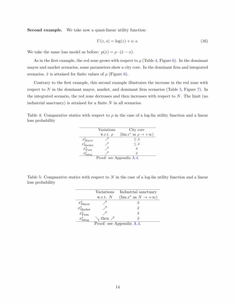
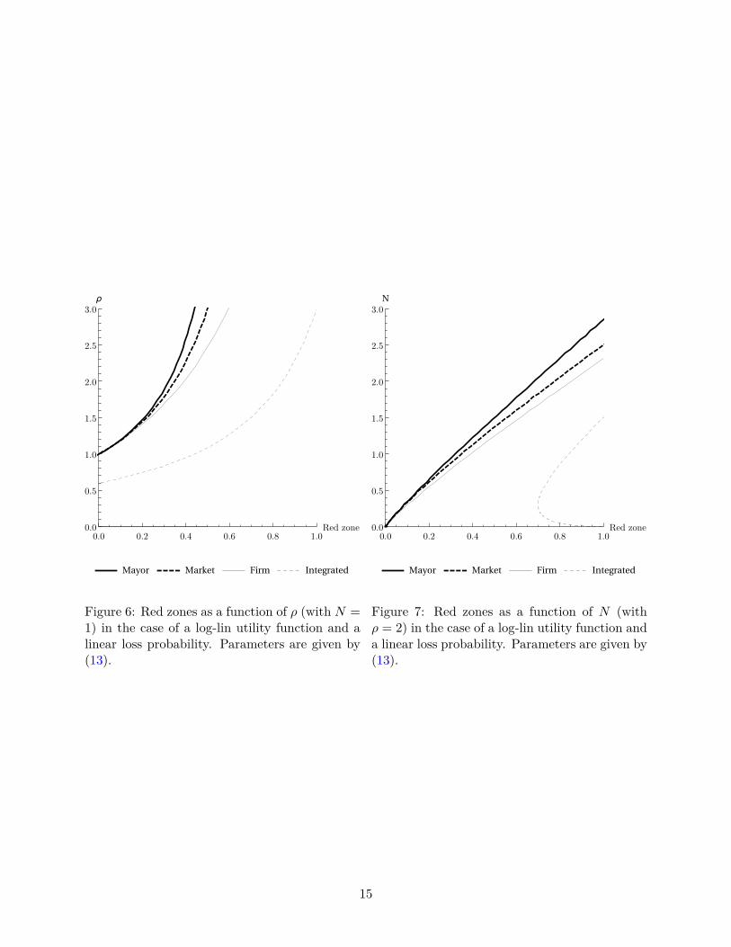
As in the first example, the red zone grows with respect to ρ (Table 4, Figure 6). In the dominantmayor and market scenarios, some parameters show a city core. In the dominant firm and integratedscenarios, x is attained for finite values of ρ (Figure 6).
Contrary to the first example, this second example illustrates the increase in the red zone withrespect to N in the dominant mayor, market, and dominant firm scenarios (Table 5, Figure 7). Inthe integrated scenario, the red zone decreases and then increases with respect to N . The limit (noindustrial sanctuary) is attained for a finite N in all scenarios.
Table 4: Comparative statics with respect to ρ in the case of a log-lin utility function and a linearloss probability
Variations City corew.r.t. ρ (lim x∗ as ρ→ +∞)
x∗Mayor ↗ ≤ xx∗Market ↗ ≤ xx∗Firm ↗ xx∗Integ ↗ x
Proof: see Appendix A.4.
Table 5: Comparative statics with respect to N in the case of a log-lin utility function and a linearloss probability
Variations Industrial sanctuaryw.r.t. N (lim x∗ as N → +∞)
x∗Mayor ↗ x
x∗Market ↗ xx∗Firm ↗ xx∗Integ ↘ then ↗ x
Proof: see Appendix A.4.
14
0.0 0.2 0.4 0.6 0.8 1.0Red zone0.0
0.5
1.0
1.5
2.0
2.5
3.0ρ
Mayor Market Firm Integrated
Figure 6: Red zones as a function of ρ (with N =1) in the case of a log-lin utility function and alinear loss probability. Parameters are given by(13).
0.0 0.2 0.4 0.6 0.8 1.0Red zone0.0
0.5
1.0
1.5
2.0
2.5
3.0N
Mayor Market Firm Integrated
Figure 7: Red zones as a function of N (withρ = 2) in the case of a log-lin utility function anda linear loss probability. Parameters are given by(13).
15

4.4 No red zone
We focus on interior solutions because they are sensitive to parameter changes. Clearly, the redzone can be null if the risk is moderate compared to the households’ taste for land and their wealth.In the dominant mayor, market, and dominant firm scenarios, the values of ρ and N for which thered zone is null are the same. Indeed, in these three scenarios, if there is no red zone, then thetransfer from the firm to the households is null; the other aspects of the game being then identical,the first order conditions are the same. Figures 8 and 9 illustrate this property for the first andsecond examples, respectively.
In the first example, the two risk factors ρ and N are complementary in all scenarios: the higherthe ρ, the higher N should be for the red zone to disappear. This case is the most intuitive (Figure8). In the second example, the two risk factors ρ and N are substitutes in all scenarios but theintegrated one: the higher the ρ, the lower N should be for the red zone to disappear (Figure9). In this example, people like relatively less space as they get richer and the firm can efficientlycounteract the demographic pressure by paying high rents on larger zones. The likeliest hypothesesare empirical questions.
1 2 3 4 5ρ
1
2
3
4
5
N
Mayor - Market - Firm Integrated
Figure 8: Boundaries in the first example.
1 2 3 4 5ρ
1
2
3
4
5
N
Mayor - Market - Firm Integrated
Figure 9: Boundaries in the second example.Note: These are the boundaries between null and positive red zones. On the left of them, the red zone isnull. Parameters are given by (13).
16

5 Conclusion
In this paper, we study the negotiation of red zones around hazardous plants. We analyze red zonesunder several scenarios that concern the distribution of bargaining power between the mayor andthe firm. We find that the stronger the bargaining power of the industrialist, the larger the red zone.To go further, we compare the reactions of these different organizations of public affairs to structuralchanges (demographic, technological, and climatic). The natural, but inexact, reasoning is that anincrease in risk should cause an extension of the red zone, whereas an increase in population shouldcause a reduction in the red zone.
We propose a thorough description of the competing effects in the general case. The willingnessto pay for land changes with the intensity of the risk but also with the actual consumption of landand the monetary transfers. The ordering of these impacts in terms of microeconomic effects enablesus to illustrate the variety of possible cases with propositions and simulations.
For given preferences, the variations in the red zone as the hazard or population size increasesdepend on the game played. Conversely, in a given scenario, these variations depend on the prefer-ences. In the scenarios where the agents who pay the cost of risk control the red zone, an increasein risk expands the red zone. This situation happens when the firm has the bargaining power and,at the other extreme, when the firm is the property of households and they decide the size of thered zone. In the other scenarios, preferences matter because the marginal rate of substitution ofhouseholds between money and space, and its variations with wealth are critical. This is the caseparticularly when the increase in risk makes the firm pay increasingly high rents to circumvent therisk. Our examples provide contrasted illustrations in that regard.
17

ReferencesBasta, C., 2009. Risk, Territory and Society: Challenge for a Joint European Regulation. Ph.D. thesis. Civil
Engineering and Geosciences / Sustainable Urban Areas Research Centre.
Bevere, L., Orwig, K., Sharan, R., 2015. Sigma Report: Natural Catastrophes and Man-made Disasters in2014: Convective and Winter Storms Generate Most Losses. Technical Report. Swiss Re.
Bevere, L., Rogers, B., Grollimund, B., 2011. Sigma Report: Natural Catastrophes and Man-made Disastersin 2010: A Year of Devastating and Costly Events. Technical Report. Swiss Re.
Blume, L., Rubinfeld, D.L., Shapiro, P., 1984. The Taking of Land: When Should Compensation be Paid?Quarterly Journal of Economics 99, 71–92.
Boxall, P.C., Chan, W.H., McMillan, M.L., 2005. The Impact of Oil and Natural Gas Facilities on RuralResidential Property Values: A Spatial Hedonic Analysis. Resource and Energy Economics 27, 248–269.
Ferrante, J., 2011. Sociology: A Global Perspective. Wadsworth Cengage Learning.
Fujita, M., 1989. Urban Economic Theory. Land Use and City Size. Cambridge University Press.
Fujita, M., Thisse, J.F., 2002. Economics of Agglomeration, Cities, Industrial Location and Regional Growth.Cambridge University Press.
Gawande, K., Jenkins-Smith, H., 2001. Nuclear Waste Transport and Residential Property Values: Estimat-ing the Effects of Perceived Risks. Journal of Environmental Economics and Management 42, 207–233.
Grislain-Letrémy, C., Katossky, A., 2014. The Impact of Hazardous Industrial Facilities on Housing Prices:A Comparison of Parametric and Semiparametric Hedonic Price Models. Regional Science and UrbanEconomics 49, 93–107.
Grossman, S.J., Hart, O.D., 1980. Takeover Bids, The Free-Rider Problem, and the Theory of the Corpora-tion. Bell Journal of Economics 11, 42–64.
Kiel, K., McClain, K., 1995. The Effect of an Incinerator Siting on Housing Appreciation Rates. Journal ofUrban Economics 37, 311–323.
Kiel, K.A., Williams, M., 2007. The Impact of Superfund Sites on Local Property Values: Are All Sites theSame? Journal of Urban Economics 61, 170–192.
McMillen, D.P., Thorsnes, P., 2003. The Aroma of Tacoma: Time-Varying Average Derivatives and the Effectof a Superfund Site on House Prices. Journal of Business & Economic Statistics 21, 237–246.
Miceli, T., Segerson, K., 2006. A Bargaining Model of Holdouts and Takings. University of ConnecticutDepartment of Economics Working Paper Series 22.
Nosal, E., 2001. The Taking of Land: Market Value Compensation Should Be Paid. Journal of PublicEconomics 82, 431–443.
Pines, D., Sadka, E., 1986. Comparative Statics Analysis of a Fully Closed City. Journal of Urban Economics20, 1–20.
Sauvage, L., 1997. L’impact du Risque Industriel sur l’Immobilier. Association des Etudes Foncières.
Schneider, S., Semenov, S., Patwardhan, A., Burton, I., Magadza, C., Oppenheimer, M., Pittock, A., Rah-man, A., Smith, J., Suarez, A., Yamin, F., 2007. Climate Change 2007: Impacts, Adaptation and Vulnera-bility. Fourth Assessment Report of the Intergovernmental Panel on Climate Change. Cambridge UniversityPress. chapter 19. pp. 779–810.
Strange, W.C., 1995. Information, Holdouts, and Land Assembly. Journal of Urban Economics 38, 317–332.
18

A Appendix
A.1 Proof of Proposition 1
We show that, for the four scenarios, the equilibrium allocation (corner or interior) (T ∗i , x∗i ) is constrainedoptimal and is the unique solution of
x∗i = 0 and MRR(0) ≤ MRSsz(ω + T∗
i
N , xN
)or
x∗i ∈ (0, x) and MRR(x∗i ) = MRSsz(ω + T∗
i
N ,x−x∗
i
N
)or
x∗i = x and MRR(x) ≥ MRSsz(ω + T∗
i
N , 0),
(17)
where the net transfer T ∗i from the firm to households is
T ∗Mayor = CR(0)− CR(x∗Mayor), (18)
T ∗Market = rx∗Market where r = MRSsz(ω + rx∗Market
N,x− x∗Market
N
), (19)
T ∗Firm such that U(ω + T ∗Firm
N,x− x∗Firm
N
)= U
(ω,
x
N
), (20)
T ∗Integ = −CR(x∗Integ). (21)
Dominant mayor, dominant firm, and integrated scenarios. For these three scenarios, wefirst check that the equilibrium of each scenario corresponds to program (8) for a particular value of Π. Thenwe show that the equilibrium allocation (T ∗i , x∗i ) is constrained optimal and is the solution of (17). We alsoprove below that the equilibrium allocation is unique.
In the dominant mayor scenario, we recognize that ΠMayor = π−CR(0). Indeed, the households captureall the benefits from risk reduction and the corresponding transfer from the firm to households is T ∗Mayor =CR(0)− CR(x∗Mayor).
In the dominant firm scenario, the firm solves a dual program where minimum utility U(ω, xN
)is guar-
anteed to the households. T ∗Firm is such that U(ω + T∗
FirmN ,
x−x∗FirmN
)= U
(ω, xN
).
In the integrated scenario, we recognize that ΠInteg = −CR(x∗Integ). Indeed, households own the firm(T ∗Integ = π) and bear the full cost of risk.
In these three cases, the constraint in (8) is convex in T and in x (it is linear in T and CR(·) is convex(CVX)). As additionally the objective is strictly quasi-concave, the Kuhn-Tucker conditions can be rearrangedto give the necessary and sufficient condition that defines the unique constrained optimum. However, thecorner solutions are not excluded.
Market scenario. For the market scenario, existence of the equilibrium allocation is proved first. Thenwe show that the equilibrium allocation (T ∗Market, x
∗Market) is constrained optimal and is the solution of (17).
The proof of existence is: The demand for land of the firm x(r) only depends on the rent. The demandof a household is sd
(w + rx(r)
N , r)where the first argument is the income and the second is the price.
Finding an equilibrium amounts to finding a root r to the equation
Nsd
(w + rx(r)
N, r
)+ x(r) = x.
The LHS will be denoted as D(r) henceforth.We show that D(·) is continuous over R: x(r) is continuous because CR(·) is convex (CVX), which implies
in turn that the households experience continuous variations in their incomes and in the prices as r increases.Their total demand for land is therefore also continuous with respect to r.
19

For r close enough to 0, the households have an unbounded demand for land, meaning that D(0+) exceedsx. For very high r, the rent paid by the firm is bounded, because it would never pay more than CR(0). Thisconstraint proves that households keep a bounded income when the price of land explodes: their demandgoes to 0 and D(r) is below x.
We now use the intermediate value theorem: the previous two paragraphs establish that there is a finiter > 0 such that D(r) = x, which implies in turn that a market equilibrium exists. However, uniqueness isnot warranted.
If r is the equilibrium rent in the market scenario, then we can assume for example that the marketallocation is interior. We have
MRR(x∗Market) = r firm’s optimality, (22)
MRSsz(ω + rx∗Market
N,x− x∗Market
N
)= r mayor’s optimality. (23)
We take ΠMarket = π − rx∗Market − CR(x∗Market) in program (8). After eliminating T by using the bindingconstraint, the first order condition of program (8) becomes:
MRR(x) = MRSsz(ω + rx∗Market + CR(x∗Market)− CR(x)
N,x− xN
). (24)
By inspection of (22) and (23), we see that x = x∗Market is a solution of (24). Because the optimum is unique,we conclude that the market scenario is efficient. This line of reasoning is similar when the market yields acorner solution.
A.2 Proof of Proposition 3
In the equations below, a stands for ρ or N . For a given red zone x, s(x, a) = x−xN , and z(x, a) = ω + T (x,a)
Nwhere
T (x, a) =
CR(0)− CR(x) (Mayor) (25)
rx s.t. r = MRSsz(ω + rx
N,x− xN
)(Market) (26)
T s.t. U(ω + T
N,x− xN
)= U
(ω,
x
N
)(Firm) (27)
−CR(x) (Integ) (28)
As stated by (17) for interior solutions, the red zones x∗ ∈ (0, x) are characterized by the equality betweenthe marginal risk reduction (MRR) and the marginal rate of substitution (MRSsz) of households.
ˆMRR(x∗, a) = MRSsz (z(x∗, a), s(x∗, a)) . (29)
By derivation of (29) with respect to a, we get(∂ ˆMRR∂x
dx∗
da+ ∂ ˆMRR
∂a
)= ∂MRSsz
∂z
(∂z
∂a+ ∂z
∂x
dx∗
da
)+ ∂MRSsz
∂s
(∂s
∂a+ ∂s
∂x
dx∗
da
). (30)
Thus
dx∗
da
(∂ ˆMRR∂x
− ∂MRSsz∂z
∂z
∂x− ∂MRSsz
∂s
∂s
∂x
)= −∂
ˆMRR∂a
+ ∂MRSsz∂z
∂z
∂a+ ∂MRSsz
∂s
∂s
∂a. (31)
20

Dominant mayor, dominant firm, and integrated scenarios. This decomposition can be usedto get the sign of dx∗/da.
Because ∂z/∂x = 1/N · ∂T /∂x > 0 and ∂s/∂x = −1/N < 0 and thanks to technical assumptions (CVX)and (ENG), the factor for dx∗/da in (31) above is negative.
Therefore the sign of dx∗/da is the sign of
∂ ˆMRR∂a
− ∂MRSsz∂z︸ ︷︷ ︸≥0
∂z
∂a− ∂MRSsz
∂s︸ ︷︷ ︸≤0
∂s
∂a. (32)
These three terms can be named and interpreted:
Risk intensification effect = ∂ ˆMRR∂a
, (33)
Income effect = −∂MRSsz∂z
∂z
∂a, (34)
Land sharing effect = −∂MRSsz∂s
∂s
∂a. (35)
The signs of ∂ ˆMRR/∂a, ∂z/∂a and ∂s/∂a are given in Table 6. But the ∂z/∂a depends on the scenarioconsidered. Thus, we can conclude in the dominant mayor, dominant firm, and integrated scenarios.
Table 6: Derivatives of ˆMRR, z and s with respect to ρ and N
All scenarios ∂ ˆMRR∂ρ = ˆMRR
ρ > 0 ∂ ˆMRR∂N = λF
x−x∗
(p(x∗)−
∫ xx∗ p(t) dtx−x∗
)≥ 0
Mayor ∂z∂ρ = CR(0)−CR(x∗)
Nρ > 0 ∂z∂N = − λS
N2 ρ∫ x∗0 f(t) dt < 0
Firm ∂z∂ρ = 0 = 0 ∂z
∂N = − x∗
N2UsUz
< 0Integrated ∂z
∂ρ = −CR(x∗)Nρ < 0 ∂z
∂N = λSN2 ρ
∫ xx∗ f(t) dt > 0
All scenarios ∂s∂ρ = 0 = 0 ∂s
∂N = − x−x∗N2 < 0
Market scenario. In the market scenario, (31) cannot be directly used: the sign of ∂z/∂x cannot bestraightforwardly computed because the rent r is endogenous. By derivation of ˆMRR = r and MRSsz = rwith respect to ρ or N , we get ambiguous expressions (available on request).
A.3 Proof of Tables 2 and 3: comparative statics on the red zone in the case ofa log-log utility function and a linear loss probability
We compute the comparative statics of x∗. In the equations below, a stands for ρ or N to economize theexposition.
Lemma 1 (Comparative statics of the size of the red zone). Consider the LHS and RHS of an equationdefining x∗. Assume that LHS decreases with respect to x∗ and that RHS increases with respect to x∗. TheLHS and RHS both depend on a parameter k.
LHS(x∗, k) = RHS(x∗, k). (36)
(i) If the LHS increases or is constant with respect to k and the RHS decreases or is constant with respectto k, then x∗ increases with respect to k.
21

(ii) If the LHS decreases or is constant with respect to k and the RHS increases or is constant with respectto k, then x∗ decreases with respect to k.
In the case of a log-log utility function and a linear loss probability, that is,
U(z, s) = log(z) + α log(s) and p(x) = ρ · (x− x), (37)
we can compute some of the red zones, their variations with respect to ρ and N , and their limits (the citycore and the industrial sanctuary) because these parameters tend to infinity. In the following, the interiorsolution of the equation that defines x∗i in scenario i is written as x∗i to have an analytic expression. Giventhe spatial constraint, the limits are calculated taking into account the fact that
x∗i = max {min {x∗i ; x} ; 0} . (38)
Dominant mayor scenario. The first order condition that characterizes the interior solution
MRR(x∗) = MRSsz(ω + CR(0)− CR(x∗)
N,x− x∗
N
), (39)
becomes
ρλFN
2 + ρλS(x− x∗Mayor) = αN
x− x∗Mayor
(ω + ρλF
2 x∗Mayor + ρλS2N x∗Mayor(2x− x∗Mayor)
). (40)
Dividing (40) by ρ enables the application of case (i) of Lemma 1 and to conclude that x∗Mayor increases withrespect to ρ. The red zone is
x∗Mayor = x− (1 + α)2(2 + α)
λFN
λS
(√1 + 8 (2 + α)
(1 + α)2λSα
λ2FNρ
(ω + ρλS
2N x2 + ρλF2 x
)− 1). (41)
x∗Mayor is always monotonic with respect to N . The red zone increases with respect to N if and only if
ρ2λ2F x
2 − 4α(α+ 2)ωρλF x− 4α(α+ 2)ω2 > 0. (42)
A city core and an industrial sanctuary exist such that:
limρ→+∞
x∗Mayor = x− (1 + α)2(2 + α)
λFN
λS
(√1 + 4α(2 + α)
(1 + α)2λS x
λFN
(λS x
λFN+ 1)− 1)
; (43)
limN→+∞
x∗Mayor = max{
11 + α
x− 2α1 + α
ω
ρλF; 0}. (44)
Market scenario. The first order condition that characterizes the interior solution
MRR(x∗) = MRSsz(ω + rx∗
N,x− x∗
N
), (45)
becomes
ρλFN
2 + ρλS(x− x∗Market) = αωN
x− (1 + α)x∗Market. (46)
Using case (i) of Lemma 1, we conclude that x∗Market increases with respect to ρ. Dividing (46) by N enablesthe application of case (ii) of Lemma 1: x∗Market decreases so with respect to N .
22
The red zone is
x∗Market = 11 + α
x
2
[2 + α− α
√1 + α
1 + α
ωN
ρλS( α1+α
x2 + λF
λS
N4 )2
]
+ λFλS
N
4
[1 −
√1 + α
1 + α
ωN
ρλS( α1+α
x2 + λF
λS
N4 )2
]. (47)
The city core and the industrial sanctuary are
limρ→+∞
x∗Market = 11 + α
x ; (48)
limN→+∞
x∗Market = max{
11 + α
x− 2α1 + α
ω
ρλF; 0}. (49)
Dominant firm scenario. The first order condition that characterizes the interior solution
MRR(x∗) = MRSsz(ω + t,
x− x∗
N
), (50)
where t is defined by
log(ω + t,
x− x∗
N
)= log
(ω,
x
N
), (51)
becomesρλFN
2 + ρλS(x− x∗Firm) = αωNxα
(x− x∗Firm)1+α . (52)
Case (i) of Lemma 1 applies and x∗Firm increases with respect to ρ. Dividing (52) by N enables the applicationof case (ii) of Lemma 1 and to conclude that x∗Firm decreases with respect to N . There is neither a city corenor an industrial sanctuary.
limρ→+∞
x∗Firm = x ; (53)
limN→+∞
x∗Firm = max{x−
(2αωxαρλF
) 11+α
; 0}. (54)
Integrated scenario. The first order condition that characterizes the interior solution
MRR(x∗) = MRSsz(ω − CR(x∗)
N,x− x∗
N
), (55)
becomesρλFN
2 + ρλS(x− x∗Integ) = αN
x− x∗Integ
(ω − ρλF
2 (x− x∗Integ)− ρλS2N (x− x∗Integ)2
). (56)
Case (i) of Lemma 1 applies and x∗Integ increases with respect to ρ. Dividing (56) by N enables the applicationof case (ii) of Lemma 1 and to conclude that x∗Integ decreases with respect to N . The red zone is
x∗Integ = x− (1 + α)2(2 + α)
λFN
λS
(√1 + 8 (2 + α)
(1 + α)2λSαω
λ2FNρ
− 1). (57)
There is neither a city core nor an industrial sanctuary.
limρ→+∞
x∗Integ = x ; (58)
limN→+∞
x∗Integ = max{x− 2α
1 + α
ω
ρλF; 0}. (59)
23

A.4 Proof of Tables 4 and 5: comparative statics on the red zone in the case ofa log-lin utility function and a linear loss probability
We use the same convention as in (38). The proof of monotonicity of the red zone with respect to ρ relies onthe direct calculation of the derivatives.
Dominant mayor scenario.
x∗Mayor =x+(λF2λS
+ 1α
)N −
√x2 + λ2
FN2
4λ2S
+ N2
α2 + λF xN
λS+ 2ωN
ρλS. (60)
limρ→∞
x∗Mayor < x iif NλF (αx−N) + αλS x2 > 0, (61)
limN→∞
x∗Mayor = x and it is attained for finite large enough N . (62)
∂x∗Mayor
∂ρ= 2αNωρ√ρ (α2N2ρλ2
F + 4α2NρxλFλS + 4λS (ρλS (N2 + α2x2) + 2α2Nω))> 0, (63)
∂x∗Mayor
∂N=αρλF + 2ρλS −
ρ(2α2Nρλ2F+4α2λS(ρxλF+2ω)+8Nρλ2
S)2√ρ(α2N2ρλ2
F+4α2NλS(ρxλF+2ω)+4ρλ2
S(N2+α2x2))
2αρλS. (64)
The proof of monotonicity with respect to N is based on three facts: the derivative changes sign only onceas N changes; it is positive for large values of N ; the explicit expression of the red zone has two zeros only,N = 0 being one of them.
Market scenario.
x∗Market = x
2 + 12
(λF2λS
+ 1α
)N − 1
2
√x2 + λ2
FN2
4λ2S
+ N2
α2 + λF xN
λS+ 4ωN
ρλS− λFN2
αλS− 2xN
α. (65)
limρ→∞
x∗Market < x iif αx−N > 0, (66)
limN→∞
x∗Market = x and it is attained for finite large enough N . (67)
∂x∗Market∂ρ
= 2αNωρ√ρ (ρ (αNλF + 2λS(N + αx)) 2 − 8αNλS (−2αω +NρλF + 2ρxλS))
> 0, (68)
∂x∗Market∂N
=αλF + 2λS −
α2Nρλ2F+2αρλFλS(αx−2N)+4λS(2α2ω+ρλS(N−αx))√
ρ(ρ(αNλF+2λS(N+αx))2−8αNλS(−2αω+NρλF+2ρxλS))
4αλS. (69)
As for the dominant mayor scenario, the proof of monotonicity with respect to N is based on three facts: thederivative changes sign only once as N changes; it is positive for large values of N ; the explicit expression ofthe red zone has two zeros only, N = 0 being one of them.
24

Dominant firm scenario. The red zone is not calculated explicitly. A system of equations defines x∗FirmandT ∗Firm, and by the theorem of implicit functions
∂x∗Firm∂ρ
= N2 (2λS(x− x∗Firm) +NλF )2 (α2(T ∗Firm + ω) +N2ρλS) > 0, (70)
∂x∗Firm∂N
= 2α(T ∗Firm(αx∗Firm +N) + αωx∗Firm) +N3ρλF2N (α2(T ∗Firm + ω) +N2ρλS) > 0. (71)
When N is large enough, T ∗ < ρNT where T is some constant: the firm always pays less than thetotal loss, hence there is an upper bound proportional to ρ and N . Therefore, we find lower bounds of thederivatives:
∂x∗Firm∂ρ
>N3λF
2(α2(ρNT + ω) +N2ρλS
) > N3λF
2(α2(NT + ω) +N2λS
) 1ρ, (72)
∂x∗Firm∂N
= N3ρλF2N (α2(T ∗Firm + ω) +N2ρλS) >
N2ρλF
2(α2(ρNT + ω) +N2ρλS
) (73)
>λF2λS
− ε for ε very small and N large enough. (74)
The fact that x∗Firm goes to infinity (i.e. reaches x) as ρ or N goes to infinity can be deduced from the aboveinequalities by using the Grönwall inequality to conclude. Consequently
limρ→∞
x∗Firm = x and it is attained for finite large enough ρ, (75)
limN→∞
x∗Firm = x and it is attained for finite large enough N . (76)
Integrated scenario.
x∗Integ =x+(λF2λS
+ 1α
)N −
√λ2FN
2
4λ2S
+ N2
α2 + 2ωNρλS
. (77)
limρ→∞
x∗Integ = x and it is attained for finite large enough ρ, (78)
limN→∞
x∗Integ = x and it is attained for finite large enough N . (79)
∂x∗Integ
∂ρ= 2αNωρ√Nρ (α2Nρλ2
F + 4λS (2α2ω +NρλS))> 0, (80)
∂x∗Integ
∂N=αλF + 2λS −
α2Nρλ2F+4λS(α2ω+NρλS)√
Nρ(α2Nρλ2F
+4λS(2α2ω+NρλS))2αλS
. (81)
Concerning the variations with respect to N , a case where the red zone is nonmonotonic for positive valuesof N has been constructed and simulated (see Figure 7).
25