neighbor list collision-driven molecular dynamics simulation for nonspherical hard particles.: ii....

Journal of Computational Physics 202 (2005) 765–793

www.elsevier.com/locate/jcp

Neighbor list collision-driven molecular dynamicssimulation for nonspherical hard particles.II. Applications to ellipses and ellipsoids

Aleksandar Donev a,b, Salvatore Torquato a,b,c,*, Frank H. Stillinger c

a Program in Applied and Computational Mathematics, Princeton University, Princeton, NJ 08544, USAb Princeton Institute for the Science and Technology of Materials, Princeton University, Princeton, NJ 08540, USA

c Department of Chemistry, Frick Laboratory, Princeton Materials Institute, Princeton University, Princeton, NJ 08544-5211, USA

Received 19 May 2004; accepted 9 August 2004

Available online 11 November 2004

Abstract

We apply the algorithm presented in the first part of this series of papers to systems of hard ellipses and ellipsoids.

The theoretical machinery needed to treat such particles, including the overlap potentials, is developed in full detail. We

describe an algorithm for predicting the time of collision for two moving ellipses or ellipsoids. We present performance

results for our implementation of the algorithm, demonstrating that for dense systems of very aspherical ellipsoids the

novel techniques of using neighbor lists and bounding sphere complexes, offer as much as two orders of magnitude

improvement in efficiency over direct adaptations of traditional event-driven molecular dynamics algorithms. The prac-

tical utility of the algorithm is demonstrated by presenting several interesting physical applications, including the

generation of jammed packings inside spherical containers, the study of contact force chains in jammed packings,

and melting the densest-known equilibrium crystals of prolate spheroids.

� 2004 Elsevier Inc. All rights reserved.

1. Introduction

In the first paper of this series of two papers, we presented a collision-driven molecular dynamics algo-

rithm for simulating systems of nonspherical hard particles. The algorithm rigorously incorporates near-

neighbor lists, and further improves the treatment of very elongated objects via the use of bounding sphere

0021-9991/$ - see front matter � 2004 Elsevier Inc. All rights reserved.

doi:10.1016/j.jcp.2004.08.025

* Corresponding author. Tel.: +1 609 258 3341; fax: +1 609 258 6878.

E-mail addresses: [email protected], [email protected] (S. Torquato).

mailto:[email protected]

766 A. Donev et al. / Journal of Computational Physics 202 (2005) 765–793

complexes. Detailed pseudocodes for the algorithm were presented, but several particle-shape-dependent

components were left unspecified. In particular, a key component of the algorithm is the evaluation of

overlap between scaled versions of two particles, such as the evaluation of the minimal common scaling

that leaves two disjoint ellipsoids nonoverlapping, or the maximal scaling of an ellipsoid which leaves it

contained within another ellipsoid. Additionally, the required procedures for predicting the time-of-collision for two moving ellipsoids, as well as processing the collision, are developed. Moreover, we discuss

generalizations to other particle shapes.

We also illustrate the practical utility and versatility of the algorithm by presenting several nontrivial

and physically relevant applications. In particular, we show that by incorporating particle growth (i.e.,

shape deformation), the proposed algorithm can generate jammed packings of ellipsoids and is superior

to previously used algorithms in both speed and particularly in accuracy. The high precision of the

event-driven approach enables us to reach previously unavailable high densities and to produce tightly

jammed ellipsoid packings with several thousand particles, even for relatively large aspect ratios [12].Additionally, the inclusion of boundary deformation allowed us to generate the densest known crystal

packings of ellipsoids [11], and here we show how the algorithm can be used to simulate a quasi-equi-

librium (adiabatic) expansion of this crystal to track its equation of state and phase behavior. We also

demonstrate how using near-neighbor lists can help monitor the particle collision history near the jam-

ming point and enable the study of force chains, previously studied only in time-driven molecular

dynamics of soft particles [3].

We present the tools necessary to rapidly evaluate overlap functions for ellipsoids in Section 2. We then

describe the missing particle-shape-dependent pieces of the algorithm in Section 3. Some performanceresults for the algorithm are shown in Section 4, particularly focusing on the use of our near-neighbor list

and bounding sphere complexes techniques. Three illustrative applications are given in Section 5.

2. Geometry of ellipses and ellipsoids

In this section, we focus exclusively on ellipsoidal particles, particularly in two (ellipses) and three (ellip-

soids) dimensions. We present all of the necessary tools to adapt the EDMD algorithm to ellipsoids. Wefirst give some introductory material, and then discuss several overlap (contact) functions for ellipsoids,

based on the work of Perram and Wertheim [30]. We then focus on calculation of these overlap functions

and their time derivatives, which is used in Section 3 to robustly determine the time-of-collision for two

moving ellipsoids. We will attempt to present most of the results so that they generalize to other dimensions

as well; however, this is not always possible. We present the basic concepts in a unified and simple manner.

Readers looking for more detailed background information are referred to [1,2].

2.1. Introduction and background

In order to deal with the rotational degrees of freedom for ellipsoids and track their orientation, as well

as their centroidal position, some additional machinery is necessary. Since very little of the notation seems

to be standard, we first present our own notational system, which attempts to unify different dimensional-

ities whenever possible. We then discuss orientational degrees of freedom and rotation of rigid bodies.

2.1.1. Notation

When dealing with rotational motions, especially in three dimensions, cross products and rotationalmatrices appear frequently. In order to unify our presentation for two and three dimensions as much as

possible, we introduce some special matrix notation. Matrix multiplication is assumed whenever products

A. Donev et al. / Journal of Computational Physics 202 (2005) 765–793 767

of matrices or a matrix and a vector appear. We prefer to use matrix notation whenever possible 1 and do

not carefully try to distinguish between scalars and matrices of one element. We denote the dot product a Æ bwith aTb, and the outer product a � b with abT.

The first notational difficulty relates to the notion of a cross product. In three dimensions, there is only

the familiar cross product

1 O

a� b ¼aybz � azbyazbx � axbzaxby � aybx

264

375 ¼ Ab; ð1Þ

where

A ¼0 �az ayaz 0 �ax�ay ax 0

264

375 ¼ �AT

is a skew-symmetric matrix which is characteristic of the cross product and is derived from a vector. We will

simply capitalize the letter of a vector to denote the corresponding cross product matrix (like A above

corresponding to a). In two dimensions however, there are two ‘‘cross products’’. The first one gives the

velocity of a point r in a system which rotates around the origin with an angular frequency x (which

has just one z component and can also be considered a scalar x),

v ¼ x � r ¼�xryxrx

� �¼ Xr; ð2Þ

where

X ¼0 �xx 0

� �¼ �XT

is a cross product matrix derived from x. The second kind of ‘‘cross product’’ gives the torque around the

origin of a force f acting at a point (arm) r,

s ¼ f � r ¼ �r� f ¼ fxry � fyrx� �

¼ FLr; ð3Þ

where

FL ¼ �fy fx½ � ¼ � FR� �T

is another cross product matrix derived from a vector (the �L� and �R� stand for left and right multiplication,

respectively). Note that in three dimensions all of these coincide, FL = FR = F, and also > ” ·. The nota-

tion was chosen so equations look simple in three dimensions, but are also applicable to two dimensions.

The wedge product generalizes the cross product in higher dimensions [20].

2.1.2. Rigid Bodies

Representing the orientation of a rigid body in a computationally convenient way has been a subject of

debate in the past [2]. A rigid body has

ur computational implementation uses a specially designed library of inlined macros for matrix operations extensively.

2 N


fR ¼d d � 1ð Þ

2¼

1 if d ¼ 2;

3 if d ¼ 3;

�ð4Þ

rotational degrees of freedom, and this is the minimal number of coordinates needed to specify the config-

uration of a hard nonspherical particle, in addition to the usual d coordinates needed to specify the position

of the centroid. In two dimensions orientations are easy to represent via the angle / between the major

semiaxes of the ellipsoid and the x axis. But in three dimensions specifying three (Euler) angles is numer-

ically unstable, and extensive experience has determined that for MD computationally the best way to rep-

resent orientations is via normalized quaternions, which in fact represent finite rotations starting from aninitial reference configuration (but see [17] for a discussion). In the case of ellipsoids this reference config-

uration is one in which all semiaxes are aligned with the coordinate axes. In two dimensions we use a nor-

malized complex number to represent orientation, but for simplicity we will sometimes use the term

‘‘quaternion’’ in both two and three dimensions. Higher dimensional generalizations are discussed in [33].

In three dimensions, normalized quaternions consist of a scalar s and a vector p,

q ¼ s; p½ � ¼ cos/2; sin

/2

� /̂

� �; ð5Þ

where /̂ is the unit vector along the axis of rotation and / is the angle of rotation around this axis, and the

normalization condition

qk k2 ¼ s2 þ pk k2 ¼ 1

is satisfied. Therefore in three dimensions we use 4 numbers to represent orientation, which seems like wast-

ing one floating-point number. It is in fact possible to represent the rotation with the oriented angle

/ ¼ //̂, which is just a vector with 3 coordinates. However, such a representation has numerical problemswhen / = 0, and also the representation is not unique. 2 More importantly, combining rotations (as during

rotational motion) does not correspond (as one may expect) to vector addition of the /�s, but it does cor-respond to quaternion multiplication of the q�s, which is fast since there is no need of repeating the trigo-

nometric evaluations. This is the reason why we also use quaternions in two-dimensions, and represent the

orientation of a particle in the plane with 2 coordinates (components of a unit complex number),

q ¼ s; p½ � ¼ cos/; sin/½ �: ð6Þ
The orthogonal rotation matrix corresponding to the rotation described by the quaternion (5) is given
with

Q ¼ 2 ppT � sPþ s2 � 1

2

� I

� �

in three dimensions, and

Q ¼s p

�p s

� �

in two dimensions, corresponding to the complex number (6). The resulting orientation after first the rota-

tion Q1 is applied and then the rotation Q2 is applied, Q12 = Q2Q1, is represented by the quaternion

product

q12 ¼ q1q2 ¼ s1s2 � p1 � p2; s1p2 þ s2p1 � p1 � p2½ � ð7Þ

ote that the quaternion representation is also not unique since �q and q represent the same orientation.


in three dimensions, and by the complex number product

3 R4 W

q12 ¼ q1q2 ¼ s1s2 � p1p2; s1p2 þ s2p1½ � ð8Þ
in two dimensions.
In this work, we are interested in particles which move continuously in time. The rate of rotation of a

rigid body is given by the angular velocity x (which can also be considered a scalar x in two dimensions), or

equivalently, the infinitesimal change in orientation is given by the infinitesimal rotation d/ = xdt. The

instantaneous time derivative of the normalized quaternion is given with 3

_q ¼ 1

2

s �pp sIþ P

� �0

x

� �

in three dimensions, and with

_q ¼ 1

2

s p

�p s

� �0

x

� �

in two dimensions. The time derivative of the corresponding rotation matrix is

_Q ¼ �QX;

and this result has was used extensively in deriving the various time derivatives related to the contact func-

tion for ellipsoids, as will be given shortly.

2.1.3. Ellipsoids

An ellipsoid is a smooth convex body consisting of all points r that satisfy the quadratic inequality

r� r0ð ÞTX r� r0ð Þ 6 1; ð9Þ
where r0 is the position of the center (centroid), and X is a characteristic ellipsoid matrix describing the
shape and orientation of the ellipsoid. The case when X ¼ 1O2 I is a diagonal matrix describes a sphere of

radius 4 O, which does not require orientation information. In the general case,

X ¼ QTO�2Q; ð10Þ
where Q is the rotational matrix describing the orientation of the ellipsoid, and O is a diagonal matrix con-
taining the major semi-axes of the ellipsoid along the diagonal. The time derivative of the matrix (10) for an

ellipsoid rotating with instantaneous angular velocity x is

_X ¼ XX� XX: ð11Þ
In Algorithm 1 we give a prescription for updating the orientation of an ellipsoid rotating with a constant
angular velocity for a time Dt.

Algorithm 1. Update the orientation of an ellipsoid rotating with a uniform angular velocity x after a time

step Dt.

1. Calculate the change in orientation qDt using /Dt = xDt in Eqs. (5) or (6).

2. Update the quaternion, q qqDt, using Eqs. (7) or (8).

3. If jiqi�1j > �q (due to accumulation of numerical errors), renormalize the quaternion, q q/iqi.

ecall that capital P denotes the cross product matrix corresponding to p.

e will use the letters r and R to denote positions of points, and therefore resort to using O when referring to radius.


2.2. Ellipsoid overlap potentials

The problem of determining whether two ellipsoids A and B overlap (have a common point) or not has

been considered previously in relation to Monte Carlo or MD simulations of hard-ellipsoid systems [1].

Here, we are concerned not only with a binary overlap criterion, but rather with a numerically efficient

way of measuring a distance 5 between the two ellipsoids F(A,B), whose sign not only gives us an overlap

criterion,

5 T

F ðA;BÞ > 0 if A and B are disjoint;

F ðA;BÞ ¼ 0 if A and B are externally tangent;

F ðA;BÞ < 0 if A and B are overlapping;

8>><>>:

but which is also continuously differentiable in the positions and orientations of the ellipsoids A and B and

is numerically stable. An additional convenient property is that F(A,B) be defined and easy to compute for

all positions and orientations of the ellipsoids. We will call such a distance function an overlap potential. Wewill also make use of an overlap potential G(A,B) for the case when ellipsoid A is completely contained

within B (for example, B can be the bounding neighborhood of A, or it can be an ellipsoidal hard-wall

container),

GðA;BÞ > 0 if A is completely contained in B;

GðA;BÞ ¼ 0 if A is internally tangent to B;

GðA;BÞ < 0 if part or all of A is outside B;

8><>:

and give such a potential below. Such potentials have not been considered before since they do not appear

in other algorithms, however, our neighbor-list EDMD algorithm for ellipsoids uses it to construct bound-

ing neighborhoods for the particles, and additionally, such a potential can be used to implement hard-wall

boundary conditions inside an ellipsoidal container.More than three decades ago, Vieillard-Baron proposed an overlap criterion based on the number of

negative eigenvalues of a certain matrix [44], and this criterion has been subsequently rediscovered [45].

It easily generalizes to two dimensions and can be used to obtain an overlap potential. We have imple-

mented and tested this overlap potential but have found it both computationally and theoretically inferior

to an overlap potential proposed by Perram and Wertheim [30]. We have therefore completely adapted the

Perram–Wertheim (PW) overlap potential and also extended it to the case of one ellipsoid contained within

another. Many other approaches are possible, for example, an approximate measure of the Euclidean dis-

tance between the surfaces of the two ellipsoids can be used [14,16,23,31]. However, the advantage of thePW approach is its inherent symmetry, dimensionless character, and most of all, its simple geometric

interpretation in terms of scaling factors.

The geometrical idea behind the Perram–Wertheim overlap potential is very simple and is based on con-

sidering scaling the size of the ellipsoids uniformly until they are in external or internal tangency. Consider

for example the case when A and B are disjoint, as illustrated in the leftmost part of Fig. 1. If ellipsoid A is

scaled by a nonnegative factor l(A) such that the centroid of B is still outside it, then there is a correspond-

ing scaling of B, l(B), which brings B into external tangency with A at the contact point rC[l(A)]. Thisscaling is a solution to a simple eigenvalue-like problem involving XA and XB. The normal vectors of Aand B at the contact point are of opposite direction, and by changing the ratio of their lengths from 0

his is not a distance in the mathematical sense.

Fig. 1. Illustration of the scaling l in the PW contact function: Left: The outer tangency potential lAB. Middle: The outer tangency

potential lB(A). Right: The inner tangency potential mB(A).


to1 we get a path of contact points going from the center of A to the center of B. It was a wonderful idea

of Perram and Wertheim [30] to parameterize this path with a scalar k 2 [0,1], and then look for the k = Kwhich makes l(A) = l(B), i.e. look for the common scaling factor lAB which brings A and B into external

tangency at the contact point rC (shown in Fig. 1), or equivalently, look for the largest common scaling

factor which preserves non-overlap. This approach is very well-suited for the case when both A and B

are particles and thus should be treated equally. Sometimes, however, ellipsoid B has a special status,

for example, it may be the bounding neighborhood of another particle. In this case we look for the scalingfactor lB(A) of A which brings A into external tangency with the fixed B (see second subsection in Section

II.C in [29]), or equivalently, the largest scaling of A which preserves non-overlap, as illustrated in the mid-

dle part of Fig. 1. A similar idea applies to the case when A is contained within B, in which case we look for

the largest scaling mB(A) of A which leaves A contained completely within B, or equivalently, which brings A

into internal tangency with B.

Using these scaling factors, we can define several overlap potentials,

F ABðA;BÞ ¼ l2AB � 1; ð12Þ

F BðA;BÞ ¼ l2BðAÞ � 1; ð13Þ

GBðA;BÞ ¼ m2BðAÞ � 1; ð14Þ

which we will refer to as the Perram–Wertheim (PW), the modified PW overlap potential, and the internal

PW overlap potential respectively. To appreciate why we use the squares of the scaling factors, consider thecase of spheres, where the PW overlap potential simply becomes

F AB ¼rA � rBj j2

OA þ OBð Þ2� 1 ¼ l2AB

OA þ OBð Þ2� 1;


which avoids the use of square roots in calculating the distance between the centers of A and B, lAB,

and is also much simpler to work with analytically. Extensive use of all three of the contact functions

(12)–(14) has been made in the implementation of the algorithm, and in particular, the building and

updating of the near-neighbor lists. The original PW overlap potential (12) is the most efficient in prac-

tice and also has the property that it is symmetric with respect to the interchange of A and B, and ispreferred over (13) unless l2

BðAÞ is needed (recall from the first paper in this series that lB(A) is needed

when using partial updates for the neighbor lists). Note that FB and GB are not defined for all positions

of the ellipsoids, namely, if the center of A is inside B, FB is not defined, and conversely, if the center of

A is outside B, GB is not defined.

2.3. Calculating the overlap potentials

In this section, we address the issue of efficiently and reliably calculating the three PW overlap potentials.We base our discussion on outlines of recipes for calculating FAB and FB in the literature [1,29,30], but focus

on detail and describe a specific computational scheme based on polynomials. Additionally, contact infor-

mation such as the point of contact or the common normal vector at the point of contact can be calculated

once the overlap potential is found.

2.3.1. Evaluating FAB

Following Perram and Wertheim, define the parametric function

fAB kð Þ ¼ k 1� kð ÞrTABY�1rAB; ð15Þ

where rAB = rB � rA, and

Y ¼ kX�1B þ 1� kð ÞX�1A : ð16Þ
It turns out that this function is strictly concave on the interval [0,1] and thus has a unique maximum at
k = K 2 [0,1], from which one can directly calculate the overlap potential:

F AB ¼ fAB Kð Þ ¼ max06k61

fAB kð Þ:

The maximum of fAB(k) can easily be found numerically using only polynomial manipulations, by making

extensive use of matrix adjoints (sometimes called adjugates) and determinants (both of which are polyno-

mials in the matrix elements). First rewrite fAB(k) as a rational function:

fAB kð Þ ¼ pAB kð ÞqAB kð Þ ¼

k 1� kð Þ aTABadj kIþ 1� kð ÞAAB½ �aAB �det kIþ 1� kð ÞAAB½ � ; ð17Þ

where

aAB ¼ X1=2B rAB and AAB ¼ X

1=2B X�1A X

1=2B :

Note that powers of X are easy to calculate because of the special form (10) and orthogonality ofQ. We havemade use of the symbolic algebra systemMaple� and its code generation abilities to generate inlined Fortran

code to form the coefficients of the polynomial adj[kI + (1 � k)A] and det[kI + (1 � k)A] for a given symmet-

ric matrix A, and this has found numerous uses when dealing with ellipsoids, such as in evaluating the coef-

ficients of the polynomials pAB and qAB in Eq. (17). The unique maximum of fAB(k) can be found by finding

the root of its first derivative, which is the same as finding the unique root of the degree-2d polynomial

hAB ¼ p0ABqAB � pABq0AB

in the interval [0,1], which can be done very rapidly using a safeguarded Newton method.


A good initial guess to use in Newton�s method is the exact result for spheres

K ¼ OA

OA þ OB;

where O is the largest semiaxis, i.e., the radius of the enclosing sphere for an ellipsoid. Additionally, oneoften has a better initial guess for K in cases when the relative configuration of the ellipsoids has not chan-

ged much from previous evaluations of FAB. Finally, a task which appears frequently is to evaluate the

overlap potential between two ellipsoids but only if they are closer than a given cutoff, in the sense that

the exact value is only needed if F AB 6 F ðcutoffÞAB , or equivalently lAB 6 lðcutoffÞAB (see for example the algorithms

for updating the neighbor lists in the first paper in this series). This cutoff can be used to speed up the proc-

ess by terminating the search for K as soon as a value fABðkÞ > F ðcutoffÞAB is encountered during Newton�smethod. Additionally, one can first test the enclosing spheres for A and B with the same cutoff and not con-

tinue the calculation if the spheres are disjoint even when scaled by a factor lðcutoffÞAB .Since almost always the value of k = K is used, henceforth we do not explicitly denote the special value K,

unless there is the possibility for confusion. The reader should keep in mind that expressions to follow are

to be evaluated at k = K. The subscript C will be used to denote quantities pertaining to the contact point.

The contact point rC of the two ellipsoids is

rC ¼ rA þ 1� kð ÞX�1A n ¼ rB � kX�1B n; ð18Þ

where

n ¼ Y�1rAB ð19Þ

is the unnormalized common normal vector at the point of contact (once the ellipsoids are scaled by the

common factor lAB), directed from A to B in this case. Here, rBC = rC � rB and rAC = rC � rA are the

‘‘arms’’ from the centers of the ellipsoids to the contact point. An important value is the curvature of

fAB at the special point k = K,

fkk ¼d2fABdk2

¼ 2rTBCY

�1rAC

k 1� kð Þ ¼ �2nTZn < 0;

where

Z ¼ X�1A Y�1X�1B ¼ X�1B Y�1X�1A ¼ kXA þ 1� kð ÞXB½ ��1:

2.3.2. Evaluating FB and GB

The evaluation of the modified outer and internal tangency PW overlap potentials FB and GB proceeds in

a similar fashion, but with a differing sign in several expressions. Here, the upper sign will denote the case of

internal tangency (GB), and the lower the case of outer tangency (FB). We proceed to give a prescription for

evaluation of these potentials without detailed explanations.

As for evaluating FAB above, first we define the parameterized function

fB kð Þ ¼ k2rTABY�1X�1B Y�1rAB; ð20Þ

as well as

gB kð Þ ¼ 1� kð Þ2rTABY�1X�1A Y�1rAB; ð21Þ

where

Y ¼ kX�1B � 1� kð ÞX�1A : ð22Þ


We then numerically look for the largest k = K in [0,1] which solves the nonlinear equation

6 In

fB kð Þ ¼ 1; ð23Þ
and then we have the desired scaling factor
GB or F B ¼ gB Kð Þ ¼ m2B � 1 or l2B � 1:

Additionally, the contact point is

rC ¼ rA � 1� kð ÞX�1A n ¼ rB � kX�1B n; ð24Þ
where the normal vector n is as in Eq. (19). An additional useful value is the slope
fk ¼dfBdk¼ 2

rTBCY�1rAC

1� kð Þ :

We can again use polynomial algebra to efficiently solve Eq. (23) using a safeguarded Newton method,by rewriting fB(k) as a rational function

fB kð Þ ¼

Pdk¼1

kpðBÞk kð Þh i2q2B kð Þ ¼ k2 adj kI� 1� kð ÞAAB½ �aABk k2

det kI� 1� kð ÞAAB½ � ¼ 1; ð25Þ

where pðBÞk and qB are polynomials, to obtain the equivalent equation

qB kð Þ

k

ffiffiffiffiffiffiffiffiffiffiffiffiffiffiffiffiffiffiffiffiffiffiffiffiffiffiPdk¼1

pðBÞk kð Þh i2s ¼ 1;

which is better suited for numerical solution. The search interval for K in this case should be taken to be

½~K; 1�, where ~K is the largest root of the degree-d polynomial qB in [0,1], which can be found exactly in both

two and three dimensions using standard algebraic methods for the solution of polynomial equations of

degree less than 5. A reasonable initial guess when evaluating GB is k ¼ ~K.Unlike the evaluation of FAB and FB, which are both rapid 6 and robust, the evaluation of GB poses

numerical difficulties due to the presence of the minus sign in Eq. (22), which can cause Y to become

singular. This happens when iY�1rABi! 0, which does occur when K! ~K. In this case, since Y is singular,its adjoint is (almost always) rank-1,

adj Y½ � ! uuT;

where u is some (eigen)vector, and the problem occurs because uTrAB! 0, yielding an apparently indeter-

minate 0/0 in Eq. (25). The limiting value of GB is mathematically well-defined even in this case, however, its

numerical evaluation is unstable, and has been a constant source of numerical problems in our implemen-

tation. One alleviating trick is to avoid explicitly inverting Y and instead the adjoint should be used,

Y�1 = adj[Y]/det[Y], where the determinant of Y can be calculated by using (23),

det Y½ � ¼ kffiffiffiffiffiffiffiffiffiffiffiffiffiffiffi~nTX�1B ~n

q;

where ~n ¼ adj½Y�rAB. Even with such precautions, we have observed numerical difficulties in the calculations

involving inner tangency of A and B. It would therefore be useful to explore alternative overlap potentials

for the case when ellipsoid A is contained within ellipsoid B, or different ways of calculating GB.

our numerical experience FAB and its time derivatives can be evaluated significantly faster.


2.4. Time derivatives of the overlap potentials

When dealing with moving ellipsoids, and in particular, when determining the time-of-collision for two

ellipsoids in motion, expressions for the time derivatives of the contact potentials are needed. We give these

expressions here without a detailed derivation. We have additionally obtained expressions for second orderderivatives, however these are not needed for the current exposition and are significantly more complicated,

and are not presented here. We use the standard dot notation for time derivatives.

2.4.1. Derivatives of FAB

Consider two ellipsoids moving with instantaneous velocities vA and vB and rotating with instantaneous

angular velocities xA and xB. For the purposes of the Lubachevsky–Stillinger algorithm, we also want to

allow the ellipsoid semiaxes to change with an expansion/contraction rate of c ¼ _O, i.e., O(t) = O(0) + ct.

We have the expected result that the rate of change of overlap depends on the projection of the relativevelocity at the point of contact, vC, along the common normal vector n,

_F AB ¼ 2k 1� kð ÞnTvC; ð26Þ

where

vC ¼ vB þ xB � rBC þ CBrBC½ � � vA þ xA � rAC þ CArAC½ �

and

C ¼ QT O�1c� �

Q:

One sometimes also needs the time derivative of k = K

_k ¼ � 2

fkk~nTvC þ nT kCBrBC þ 1� kð ÞCArAC½ � þ k 1� kð ÞnTZ xB � xAð Þ � n½ �

�; ð27Þ

where

~n ¼ kY�1rBC þ 1� kð ÞY�1rAC:

2.4.2. Derivatives of FB and GB

In this case we have:

_GB or _F B ¼ �2 1� kð ÞnTvC ð28Þ
and
_k ¼ � 2kfk

rTBCY�1vC þ rTACY

�1CBrBC � rTBCY�1CArAC

� �� k 1� kð ÞnTZ xB � xAð Þ � n½ �

�: ð29Þ

3. EDMD for ellipses and ellipsoids

Having developed the necessary tools for dealing with overlap between ellipses and ellipsoids in Section

2, we can now complete the description of the EDMD algorithm. We first discuss the fundamental step of

predicting collisions between moving ellipsoids, and then explain how to process a binary collision betweentwo ellipsoids.


3.1. Predicting collisions

The central step in event-driven MD algorithms is the prediction of the time-of-collision for two moving

particles, as well as the time when a particle leaves its bounding neighborhood. This is also the most time-

consuming step, especially for nonspherical particles. Although general methods can be developed for par-ticles of arbitrary shape [43], efficiency is of primary concern to us and we prefer specialized methods which

utilize the properties of ellipsoids, in particular, their smoothness and the relative simplicity of the time

derivatives of the overlap potentials given in Section 2.4. In three dimensions, we restrict consideration

to ellipsoids with a spherically symmetric moment of inertia, i.e., ellipsoids with equal moment of inertia

around all axes. This is because the force-free motion of general ellipsoids, as well as their binary collisions,

are very complex to handle. For example, the angular velocity is not constant but oscillates in a complex

manner. It is not hard to adapt the algorithms presented here to ellipsoids with several different moments

of inertia, at least in principle.Essentially, predicting the collision time tc between two moving ellipsoids A(t) and B(t) consists in find-

ing the first non-zero root of the overlap potential F(t) = F[A(t),B(t)], where F can be either one of FAB, FB

or GB, depending on the type of collision and the choice of the potential. Formally:

Fig. 2.

grid, w

zero cr

tc ¼ min t;

such that F ðtÞ ¼ 0 and t P 0;ð30Þ

where F(t) is a smooth continuously differentiable function of time, as illustrated in Fig. 2. This kind of first

root location problem has wide applications and has been studied in various disciplines. For a general non-

polynomial F(t), its rigorous solution is a very hard problem and requires either interval methods [6] or rig-

orous under/over estimation of F(t) based on knowledge of exact bounds on the Lipschitz constant of _F(and possibly of F) [10]. These methods are rather complex and are focused on robustness and generality,

rather than efficiency. For particular forms of F(t), rigorous algebraic methods may be possible, such as for

0 0.2 0.4 0.6 0.8 1t

0

0.5

1

1.5

2

f(t)

The time evolution of the overlap function FAB(t) during an ellipse collision. The overlap function is evaluated on an adaptive

hich has a smaller time step when FAB changes rapidly, and a larger step when it is relatively smooth. The tracing stops when a

ossing is detected.


example the prediction of time of collision of two needles (infinitely thin hard rods) [18], and possibly

spherocylinders. However, this requires a considerable algebraic complexity and is not easy to adapt to

a new particle shape, especially ellipsoids, for which there is not even a closed-form expression for the

overlap potential.

In particular, the very elegant method for determining the time of collision of two needles proposed in[18] is related to the one proposed in [10], and at its core is the need to determine a good local or global

estimate of the Lipschitz constant of _F [10], i.e., an upper bound on j€F j (these are used to construct rigorous

under- or over-estimators of F(t)). Such a global upper bound has been derived for the case of needles [cf.

Eq. (20) in [18]], but for ellipsoids the expression for €F (which we do not give here) is very complex and we

have not been able to generalize the approach in [18]. As discussed in [10], significantly better results are

obtained when local estimates of the Lipschitz constant of _F are available (i.e., upper bounds on j€F j overa relatively short time interval), and this seems an even harder task. Nevertheless, it is a direction worth

investigating in the future.For the purpose of EDMD, it is sufficient only to ensure that an interval of overlap [tc,tc + Dtc] is not

missed if

mintc6t6tcþDtc

F tð Þ < ��F ;

where �F is some small tolerance, typically 10�4–10�3 in our simulations, or alternatively, if Dtc > �t. The useof �F is preferable because it is dimensionless with a scale of order 1. This essentially means that it is per-missible to miss grazing collisions, i.e., collisions in which two ellipsoids overlap for a very small amount

and/or for a very short time. It certainly is not productive to try to decide if two nearly touching particles

are actually overlapping more accurately then the inherent numerical accuracy of F(t). The choice of �F is

determined by the relative importance of correctness versus speed of execution, as well as the stability of the

simulation. A large �F can lead to unrecoverable errors in the event-driven algorithm, such as runaway

collisions or increasing overlap between particles.

Homotopy methods can be used to solve problems such as (30). They typically trace the evolution of the

root of an equation (starting from t = 0 in this particular case) as the equation is deformed from an initialsimple form to a final form which matches F(t) = 0 [46]. An ordinary differential equation (ODE) solver can

be used for this purpose. An essential component in these methods is event location in ODEs, namely, meth-

ods which solve an ODE for a certain variable f(t) and determine the first time that f(t) crosses zero [34,35].

We have tested a (simple) ODE-based homotopy method for solving (30), however since the problem at

hand is one-dimensional, one can directly apply ODE event location to f(t) ” F(t), using an absolute toler-

ance of �F for the ODE solver, and locate the first root tc directly more efficiently.

The ODE to solve is given by Eqs. (26) or (28). However, also needed is k(t), and one has the option

of either explicitly evaluating k at each time step (reusing the old value of k as an initial guess), or alsoincluding k(t) in a system of ODEs using Eq. (27) or (29). The second option has the advantage that one

no longer needs to explicitly evaluate k (other than at the beginning of the integration), however it has

the additional cost of two variables instead of one in the ODE solver, which additionally leads to smaller

time steps in the ODE integrator. Our numerical experiments have indicated that at least in two and

three dimensions it is somewhat advantageous to explicitly evaluate k and only include F(t) in the

ODE. This may be reversed for different particle shapes, depending on the relative complexity of evalu-

ating k versus evaluating _k.Once k is evaluated however, very little extra effort is needed to evaluate F explicitly, so it seems some-

what pointless to solve an ODE for F(t). We have developed a method with a similar structure to ODE

integration, but which uses explicit evaluation of both F and _F . The basic idea is to take a small time step

Dt, evaluate both F and _F at the beginning and end of the step, and use these values to form a cubic Hermite

interpolant ~F ðtÞ of F(t) over the interval Dt. A theoretically supported estimate for the absolute error of the


interpolant can be obtained by comparing the interpolant ~F and F at the midpoint of the time step, and this

error can be used to adaptively increase or decrease the size of the step so as to keep the absolute error

within �F. This is illustrated in Fig. 2. When the interpolant crosses the F = 0 axes, the first root of the inter-

polant is used as an initial guess in a safeguarded Newton algorithm to find the exact root tc. The initial

time step Dt needs to be sufficiently small to make the initial error estimate valid, and can easily be obtainedby estimating a time-scale for the collision from the sizes and velocities of the particles involved in the col-

lision. Even if this initial guess is conservative, the algorithm quickly increases the step to an appropriate

value. We will refer to this algorithm as trace event location, since the function F(t) is explicitly traced until a

zero-crossing is found.

There are several details one needs to be attentive to when predicting collisions inside an EDMD algo-

rithm. For example, some pairs of particles may already be overlapping by small amounts after having col-

lided. In this case one can look at the sign of _F to decide whether the two particles are about to have a

collision or just had a collision. Two particles can have a collision after having collided without an interven-ing collision with third party particles. This can always happen for aspherical particles, as noted in [18], and

it can also happen for spheres when boundary deformations are present (since the particles travel along

curved paths), however, it cannot happen for spheres in traditional EDMD algorithms. If the initial F is

very close to zero, an additional safety measure is to add a small positive correction to F to ensure that

it is sufficiently far from zero at the beginning of the search (as compared to the accuracy in the evaluation

of F(t)). In particular, such precautions are necessary at very high densities (i.e., near jamming).

3.1.1. Predicting collisions for ellipsoids

We sketch the procedure for predicting collisions between two moving ellipsoids in Algorithm 2. Fea-

tures in Algorithm 2 include limiting the number of steps in the event location algorithm to avoid wast-

ing resources on predicting collisions that may never happen, as well as allowing the exact prediction to

fail. This algorithm first uses collision prediction for the bounding (or contained) spheres, in order to

eliminate obvious cases when the particles do not collide, and to identify a short search interval for

the event location by calculating the time interval during which the enclosing spheres overlap. Recall that

when the boundary is not deforming this step entails solving a quadratic equation, while it involves solv-

ing a quartic equation when the lattice velocity is nonzero. In this context not only the first root of thisquadratic/quartic equation needs to be determined, but also the second one, giving the interval of over-

lap. It may be possible to further improve the initial collision prediction step by using a bounding body

other than spheres, for example, oriented bounding boxes (orthogonal parallelepipeds) [15,21]. However,

orientational degrees of freedom need to be eliminated since they are too hard to deal with because of the

appearance of trigonometric functions. For example, the bounding body can be a cylinder whose axis is

the axis of rotation of the ellipsoid and whose radius and length are sufficient to bound the rotating ellip-

soid for all angles of rotation.

An important problem we have encountered in practice is the numerical evaluation of GB when pre-dicting the time of collision of an ellipsoid with its bounding neighborhood. Namely, as the particles

move, it is highly likely that a point where Y is singular will be encountered. At such points the eval-

uation of GB is numerically unstable and often leads to unacceptably small time steps. We have dealt

with this problem in an ad hoc manner, by simply trying to skip over such points, so that the search

for a collision can be continued, but a more robust and systematic approach may be possible.

Algorithm 2. Predict whether two moving ellipsoids overlap during the time interval [0,T] by more than

�F, and if yes, calculate the time of collision tc 2 [0,T]. Essentially the same procedure can be used to

determine the time a particle A collides with its bounding neighborhood B. If the prediction cannot be

verified, return a time ~tc < tc before which a collision will not happen. Also return k at the time of

collision if desired.


1. For all intervals of overlap of the bounding spheres of A and B (or for all intervals during which the

bounding sphere of A intersects the shell between the contained and bounding sphere of its bounding

neighborhood B), [tstart,tend], starting from t = 0 and in the order of occurrence, do:

(a) If tstart > T, return reporting that no collision can happen.

(b) Set tend min{T,tend}.(c) Update the ellipsoids to time tstart, and evaluate the initial F and k.(d) If F < � (ellipsoids are overlapping or nearly touching), then evaluate _F and:

i. If _F P 0 then set F � (the ellipsoids are moving apart),

ii. Else return tc = tstart (the ellipsoids are approaching).

(e) Use trace event location to obtain a good estimate of the first root of F(t) during the interval [tstart,tend],

putting a limit on the number of time steps (for example, in the range 100–250). If no root crossing is

predicted, continue with the next interval in step 1. If the search terminated prematurely, then return

the last recorded time ~tc ¼ t.(f) Bracket the estimated first root of F(t) and refine it using a safeguarded Newton�s method (this may fail

sometimes).

(g) If the root refinement failed, set tend 12ðtstart þ tendÞ, repeat step 1c and go back to step 1e (attempt to

at least find a valid ~tc).2. Return reporting that no collision will happen.

3.2. Processing binary collisions

The steps necessary to process a binary collision between two hard particles are similar for a variety of

particle shapes, and essentially involves exchanging momentum between the two particles. We give a recipe

for colliding ellipsoids with a spherically symmetric moment of inertia in Algorithm 3. To determine thingslike the pressure it is useful to maintain the collisional contribution to the stress rc [28], which is a suitable

average of the exchange of momentum over all collisions.

Algorithm 3. Process a binary collision between ellipsoids i and (j,v). Assume that the particles havealready been updated to the current time t, and that k at the point of collision is supplied (i.e., it has been

stored for particle i, and also 1 � k in particle j, when this collision was predicted).

1. Calculate the Euclidean positions and velocities of particles rA, rB, vA and vB, as well as their angular

velocities xA and xB.

2. Find the contact point rC and normal velocity at the point of contact vn ¼ n̂TvC, using the supplied k.3. If vn > 0, then return without further processing this (most likely grazing) mis-predicted collision.

4. Calculate the exchange of momentum between the particles DpAB ¼ DpABn̂,

DpAB ¼ 2vn1

mAþ 1

mBþ rCA � n̂k k

IAþ rCB � n̂k k

IB

� �1;

where m denotes mass and I moment of inertia.

5. Calculate the new Euclidean velocities of the particles,

vA vA �DpABmA

n̂;

vB vB þDpABmB

n̂;


as well as the new angular velocities

xA xA �DpABIA

rCA � n̂ð Þ;

xB xB þDpABIB

rCB � n̂ð Þ:

Optionally update any averages that may need to be maintained (such as average kinetic energy) to

reflect the change in the velocities.

6. Record the collisional stress contribution

rc rc � DpAB rABn̂T

� �:

7. If using NNLs, record information about the collision that is being collected for the interaction between i

and (j,v), such as an accumulation of the total exchanged momentum for this interaction, total number

of collisions for this interaction, etc.

4. Performance results

In this section, we present some results for the performance of the algorithm. Many previous publications

have given performance results for EDMDfor spheres, andmost of these results apply to our algorithm.Exactnumbers depend critically on details of the coding style, programming language, compiler, architecture, etc.,

and are not reported here. Rather, we try to get an intuitive feeling of how to choose the various parameters of

the simulation to improve the practical performance. Our main conclusion is that using NNLs is significantly

more efficient than using just the cell method for particles with aspect ratio significantly different from one

(greater than 2 or so) or at sufficiently high densities. Additionally, using BSCs offers significant efficiency

gains for very prolate particles, for which good bounding sphere complexes can easily be constructed.

As derived in [37], when only the cell method is used, optimal complexity of the hard-sphere EDMD

code is obtained when the number of cells is of the order of the number of particles, Nc = H(N), withasymptotic complexity O(log N) per collision, which comes from the event-heap operations. In practice

however the asymptotic logarithmic complexity is not really observed, and instead to a very good approx-

imation the computational time expanded per processed binary collision is constant for a given aspect ratio

a at a given density, for a wide range of relative densities (volume fractions) u. Even though in principle the

basic EDMD algorithm remains O(log N) per collision, our aim is to improve the constants in this asymp-

totic form, and in particular, their dependence on the shape of the particle (in particular, the aspect ratio a).It is important to note that on modern serial workstations, the EDMD algorithm we have presented here

is almost entirely CPU-limited, and has relatively low memory requirements, even when using NNLs andBSCs. Floating point operations dominate the computation, but memory traffic is also very important. In

our implementation, simulating ellipsoids is about an order of magnitude slower than simulating spheres,

even for nearly spherical ellipsoids, simply due to the high cost of the collision prediction algorithm (the

same observation is reported in [18]) and increased memory traffic. For example, on a 1666 MHz Athlon

running Linux, our Fortran 95 implementation uses about 0.1 ms per sphere collision for a wide range of

system sizes and densities. With all the improvements described in this paper, and in particular, the use of

NNLs and BSCs, our implementation uses about 2 ms per ellipsoid collisions for prolate spheroids, and

about 2–4 ms for oblate spheroids at moderate densities for a wide range a = 1–10. Including boundarydeformations, i.e., solving quartic instead of quadratic equations when predicting binary collisions, slows

down the simulation for spheres by about a factor of 2.5 (we use a general quartic solver, and better results

may be obtained for a specialized solver).


4.1. Tuning the NNLs

We have performed a more detailed study of the performance of the algorithm when NNLs are used,

since this is a novel technique and has not been analyzed before. We perform an empirical study rather then

a theoretical derivation because such a derivation is complicated by the fact that the neighborhoods evolvetogether with the particles, and because the numerous constant factors or terms hidden in the asymptotic

expansions of the complexity actually dominate the practical performance.

Computationally, we have observed that it is good to maximize the number of cells Nc, even at relatively

low density u � 0.1, especially for rather aspherical particles. This is because binary collision predictions

become much more expensive than predicting or handling transfers, and so the saving in not predicting col-

lisions unnecessarily offsets the higher number of transfers handled. Consistent with the results reported in

[37], we observe that the number of checks due to invalidated event predictions is comparable and some-

times slightly larger than the number of collisions processed, and this suggests that additional improve-ments in this area might increase performance noticeably.

We have tested both methods for updating the neighbor lists, the complete and the partial update. A

complete update/rebuild of the near neighbor lists after they become invalid is the traditional approach in

most TDMD algorithms appearing in the literature. Since MD is usually performed on relatively homo-

geneous systems, when one particle displaces by a sufficient amount to protrude outside of its bounding

neighborhood, most particles will have displaced a significant amount, and so rebuilding their NNLs is

not so much of a waste of computational effort. The main advantage of this approach is that it can be

used to build NNLs when a good estimate of lcutoff is not available, but rather a bound on the numberof neighbors per particle Ni is provided (this is very useful, for example, in the very early stages of the

Lubachevsky–Stillinger algorithm, when particles grow very rapidly). Additionally, the algorithm for

rebuilding the lists is simpler and thus more efficient. Finally, a complete rebuilding of the NNLs yields

neighbor lists of higher quality, in the sense that the structure of the network of bounding neighborhoods

is better adapted to the current configuration of the system and thus the size of the neighborhoods is

maximal.

The algorithm for partial updates on the other hand is more complicated, and to our knowledge has

not been used in MD codes. It requires using dynamic linked lists, and it will in general yield smaller aver-age neighborhood size than a complete update, since the particle whose NNL is being updated must ad-

just its list without perturbing the rest of the NNLs. Note that at the beginning the NNLs must be

initialized by using a complete update. The main advantage of the partial update scheme is that it is more

flexible in handling nonisotropic systems or the natural fluctuations in an isotropic one. Just because one

particle happened to move fast and leave its neighborhood does not mean that all particles move that fast.

This is especially true at lower densities where clustering happens. In clusters particles have more colli-

sions per unit time and thus require fewer updates of the NNLs, but outside clusters particle move large

distances without collisions and thus require more frequent updates of their NNLs. In this sense partialupdates are local in nature while complete updates are global. We have indeed observed that in most cases

it is advantageous to use partial updates, rather then the traditional complete updates.

The first and most important test is to determine whether using near neighbor lists offers any advantages

over using just the cell method. The following intuitive arguments seem clear:

At very high densities, when the system of particles is nearly jammed [42], using NNLs is optimal,

regardless of the aspect ratio of the particles. This is because the particles move very little while they col-

lide with nearly the same neighbor particles over and over again (see Fig. 8). Therefore near jamming theNNLs are rarely updated and by predicting the collisions only with the particles with which actual col-

lisions happen significant savings can be obtained. However, as the density is lowered, the lists need to be

updated more frequently and the complexity of using NNLs becomes significant.


At very low densities the cell method is faster, even for very aspherical particles. This is because a particle

will have many collisions with the bounding neighborhoods before it undergoes a binary collision, so

that the cost is dominated by the cost of maintaining the NNLs instead of processing collisions.

The more aspherical the particles, the more preferable the NNL method becomes compared to the cell

method. This is because for very elongated particles at reasonably high densities there will be many par-ticles per cell so using the cell method will require predicting many binary collisions that will never

happen, while the NNL method will predict collisions with significantly fewer (truly) neighboring parti-

cles. For large a, the dominating cost is that of rebuilding the NNLs (since this step uses the cells), and

therefore the primary goal becomes to minimize the number of NNL updates per number of binary col-

lisions processed, as well as to improve the efficiency of the NNL rebuild, i.e., using BSCs.

Our experimental results shown in Fig. 3 support all of these conclusions. We show the ratio of the CPU

time expanded per processed binary collision for the NNL method and for the traditional cell method. Weshow results for equilibrium systems of prolate spheroids of aspect ratios a = 1, 3 and 5 at densities u = 0.1,

0.3, 0.5 and 0.6. Note that hard spheres jam in a disordered metastable state at around u = 0.64, and that

for the case a = 5 we use u = 0.55, since the jamming density is slightly lower than 0.6 for this aspect ratio

[12]. In Fig. 3(a) we show the relative slowdown caused by using NNLs for the systems for which using the

cell method is better. In Fig. 3(b) we show the relative speedup obtained by using NNLs for the systems for

which it is better to use NNLs. Both the results of using partial and complete updates are shown.

As explained in the first part of this series of papers, we use two techniques to limit the number of neigh-

bors that enter in the NNLs. The first one is to simply use the upper bound on the number of neighbors(interactions) Ni to choose only the nearest Ni neighbors per particle, and the second one is to choose a

relatively small cutoff lcutoff for the maximal size of the bounding neighborhood NðiÞ (compared to the

size of the particle i). In practice, only the second approach can be used with partial updates. This is because

partial updates must work under the limitations of doing as little change to the NNLs as possible, and this

requires that there be enough room to add and remove interactions from the lists as necessary. So when

using partial updates one must set lcutoff to a reasonable value and then set Ni to be larger then the maximal

number of neighbors a particle will have given the cutoff lcutoff and an unlimited Ni. Reasonable values for

spheres and not too aspherical particles are to set lcutoff so that on average each particle has about 5–7neighbors in two or 11–15 neighbors in three dimensions (the kissing number for spheres is 6 in two and

12 in three dimensions), while setting Ni at about 10 in two and 20 in three dimensions.

Since we wish to compare partial and complete updates, we change lcutoff and always set Ni to a suffi-

ciently high number (which grows sharply with lcutoff), and compare partial and complete updates in Fig. 3.

As expected, there is an optimal value of lcutoff which is larger for complete updates (for which NNL

updates are significantly more expensive) and also at lower densities. Note however that sometimes the

computation speed may change discontinuously as lcutoff is increased because at some point more than

first-neighbor cells need to be searched during the NNL update. Important observations to note includethe fact that tuned partial NNL updates almost always outperform tuned complete updates, and are thus pre-

ferred. Another useful observation is that the computation time is not very sensitive to the exact value of

lcutoff. Finally, note that as much as an order of magnitude of improvement is achieved for rather aspherical

particles at high densities by using the NNLs. This would be even more pronounced for larger aspect ratios

such as a = 10.

For large aspect ratios, the dominant cost is that of rebuilding the NNLs, during which many particle

pairs need to be tested for neighborhood. Therefore, the most important factor for the speed of the simu-

lation is how many particles need to be examined as potential near neighbors of a given particle i whenrebuilding NNL(i). If bounding spheres are not used, this number is proportional to the number of particles

that can fit in a cell of length a, i.e., a cube of volume a3. For prolate spheroids this number is proportional

to a2, but for oblate ones it is only proportional to a. Therefore the simulation of, for example, a = 10, is

0 0.25 0.5 0.75 1 1.25 1.5

Cutoff (µcutoff -1)

0

1

2

3

4

5

6

7

8

9

10

Slow

dow

n(C) α=1, φ=0.3(P) α=1, φ=0.3(P) α=3, φ=0.1(C) α=3, φ=0.1(C) α=1, φ=0.5(P) α=5, φ=0.1(C) α=5, φ=0.1

0 0.1 0.2 0.3 0.4 0.5 0.6 0.7 0.8

Cutoff (µcutoff -1)

10

8

6

4

2

0

12

Spee

dup

(P) α=1, φ=0.5(P) α=1, φ=0.6(C) α=1, φ=0.6(P) α=3, φ=0.3(C) α=3, φ=0.3(P) α=3, φ=0.5(C) α=3, φ=0.5(P) α=3, φ=0.6(C) α=3, φ=0.6(P) α=5, φ=0.3(C) α=5, φ=0.3(P) α=5, φ=0.5(C) α=5, φ=0.5(P) α=5, φ=0.55(P) α=5, φ=0.55

(a)

(b)

Fig. 3. Performance results for using NNLs in addition to the traditional cell method for a variety of aspect ratios a and densities u for

prolate spheroids, with both partial (P) or complete (C) updates.


prohibitively expensive for prolates, but not for oblates. As the results in Fig. 4 demonstrate, using BSCs

significantly increases the speed of processing collisions for very prolate spheroids. In this figure we show

the approximate speedup obtained by using BSCs for tuned partial updates for a range of moderate den-sities and a range of aspect ratios. As expected, at large densities there are very few updates to the NNLs

and therefore using BSCs does not offer a large speedup. For oblate spheroids in the same range of aspect


ratios, using BSCs does not offer computational savings, and therefore we do not show any performance

results. However, it is important to note that when using NNLs (at sufficiently high densities) and BSCs

(at sufficiently high aspect ratios) the actual (tuned) processing time per collision is approximately the same

for any ellipsoid shape in this range of aspect ratios, somewhere in the range 1–5 ms per binary collision in

our implementation. Therefore, for practical purposes, we feel that the algorithms presented in this papercan handle a wide range of ellipsoid shapes very well.

With the use of BSCs, prolate ellipsoids are handled much better and the scaling reduced to nearly inde-

pendent of a (note that one needs to examine a bounding spheres per particle, which is much less expensive

than looking at neighbor particles, but still not free), as we have demonstrated above. It remains a challenge

to find a technique that will also reduce the scaling to nearly independent of a for oblates as well. Addition-

ally, it is important to develop a theoretical analysis of the performance of the novel steps in the algorithm,

and in particular, to give estimates of the number of particles which need to be examined when building the

NNLs (per particle), the number of NNL updates which need to be processed per binary collision (perparticle).

4.1.1. Automatic tuning of lcutoffIt is important to note that it is possible to automatically tune lcutoff during the course of the sim-

ulation, at least in a rough way, so that the optimal computation speed is approached. This is very

important in the Lubachevsky–Stillinger packing algorithm, since there the density is not constant

but rather increases until jamming is reached. Clearly in the beginning a larger lcutoff is needed, while

near the jamming point lcutoff can be set very close to 1. By monitoring the fraction of events which arecollisions with a bounding neighborhood, and other statistics, one can periodically adaptively increase

or decrease lcutoff during the course of the simulation. We have successfully used such techniques to

speed the process of obtaining hard-particle packings, for both spheres and ellipsoids, especially for

elongated ellipsoids, but do not report details here.

0.1 0.2 0.3 0.4 0.5Density φ

0

1

2

3

4

5

6

7

8

Spee

dup

α=2α=4α=6α=8α=10

Fig. 4. Performance results for using BSCs for prolate spheroids at low to moderate densities. Using BSCs does not appear to offer

computational savings for oblate spheroids in the same a range.


5. Applications

In this section, we present three interesting physical investigations that could not have been undertaken

without the algorithm presented in this series of papers. In Section 5.1, we illustrate how collision-driven

molecular dynamics can be used to generate tightly jammed packings of ellipsoid with densities far surpass-ing previously achieved ones. In Section 5.2, we show equation-of-state curves for quasi-equilibrium melt-

ing of an unusually dense crystal ellipsoid packing [11]. Finally, in Section 5.3, we show how the near

neighbor lists can be used to monitor the collision history near the jamming point and to observe contact

force chains.

5.1. Generating jammed packings

We have used our collision-driven MD algorithm to implement a generalization of the Lubachevsky–Stillinger sphere packing algorithm [24,25] for ellipses and ellipsoids [12]. The method is a hard-particle

molecular dynamics (MD) algorithm for producing dense disordered as well as ordered packings. Small

ellipsoids are randomly distributed and randomly oriented in a box with periodic boundary conditions

and without any overlap. The ellipsoids are given velocities and their motion followed as they collide elas-

tically and also expand uniformly, using the event-driven algorithm. After some time, a jammed state with a

diverging collision rate and maximal density is reached. Based on our experience with spheres [22], we be-

lieve that our algorithm produces final states that are jammed, an in particular, that are collectively jammed.

In short, a collectively jammed configuration of particles is one in which no subset of particles can simul-taneously be continuously displaced so that its members move out of contact with one another and with the

remainder set [13,42]. The resulting packings are significantly denser that have previously been obtained for

ellipsoids using RSA, sedimentation, or shaking (MC-like) packing protocols [4,5,7,36]. High packing den-

sities have been obtained for spherocylinders using a force-biased MC method [47], however we believe that

these packings are not truly jammed. Additionally, spherocylinders cannot be oblate or spherically

asymmetric.

Several features of the molecular dynamics algorithm are necessary for the success of this packing proto-

col. First, provisions need to be made to allow time-dependent particle shapes, and we have explicitly in-cluded them in the treatment in Section 2.4. Most importantly, a very high accuracy collision resolution is

necessary at very high densities, especially near the jamming point. For this reason, a time-driven approach

cannot be used to generate jammed packings, and special care needs to be taken to ensure high accuracy of the

overlap potentials and the time-of-collision predictions, as is done withNewton refinement in our algorithms.

Finally, the use of neighbor lists significantly improves the speed of the algorithm since most computation is

expended on the last stages of the algorithm when the particles are almost jammed and the use of neighbor

lists is optimal (particularly combined with adaptive strategies for controlling lcutoff). Including a deforming

boundary in the algorithm additionally allows for a Parinello–Rahman-like adaptation of the shape of theunit cell, which leads to better (strictly jammed [13,42]) packing of the particles (see Section 5.2).

We have also implemented a hard-wall spherical boundary in our algorithm, for the purpose of compar-

ing our packings with experimental packings of MM candies and/or manufactured ellipsoids in spherical

containers. The full results of these investigations will be presented in forthcoming publications [26], and

here we just give an indication of the possibilities. To save time and implementation effort, we used lattice

boundaries (without periodic boundary conditions) and employed a trick to implement the spherical

boundary. Specifically, we put a spherical container inside a cube and then added special code in the han-

dling of the boundary conditions to predict and process collisions with the hard walls. This was not difficultto do because the spherical container is a special case of an ellipsoid and we already have well-developed

tools to deal with collisions between a small ellipsoid contained within a larger one, as presented in

Section 2.2. In fact, implementing true flat hard walls is more difficult for ellipsoids as it necessitates the

Fig. 5. A packing of N = 1000 ellipsoids with aspect ratios 0.8:1:1.25 inside a spherical container. A cube enclosing the sphere is used as

a pseudo-boundary for the purposes of the cell method. The radial density profile of a larger packing is shown in Fig. 6.


development of new overlap potentials. Fig. 5 shows one of our ellipsoid packings with an unusually high

density. The properties of this computer-generated packing compare very well to actual experimental data.

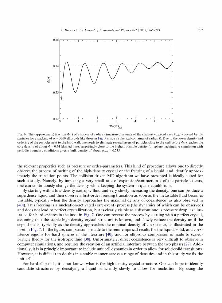
In Fig. 6 we show how the packing density varies with the radial distance, 7 clearly illustrating the layering

of the particles near the hard walls and also the fact that the density inside the core of the container has aremarkable value of about 0.74, which closely matches results obtained using periodic boundary conditions

and experimental results [12,26].

5.2. Melting dense ellipsoid crystals

Hard-particle systems are athermal, and the thermodynamic properties are solely a function of the den-

sity (volume fraction) / [1]. It is well-known that in three dimensions hard-sphere systems have a stable

low-density fluid (isotropic) phase and a stable high-density solid (face centered cubic, FCC, crystal) phase,with a first-order phase transition at intermediate densities [41]. Determining the exact transition densities is

rather difficult and requires evaluating free energies via thermodynamic integration [19]. Nevertheless, the

first-order phase transitions can be directly observed in molecular dynamics simulations, and the relevant

dynamics (nucleation or relaxation) studied. In MD, one usually studies equilibrium properties by starting

with a nonequilibrium system at a given density and then allowing it to equilibrate for a sufficiently long

time. An alternative is to very slowly change the density in a quasi-equilibrium manner while tracking

7 This is an approximation to the true density since it is rather nontrivial to exactly evaluate the volume of intersection of two

ellipsoids.

0 1 2 3 4 5 6

(R-r)/Omin

0.72

0.73

0.74

0.75

Φ(r

)

Fig. 6. The (approximate) fraction U(r) of a sphere of radius r (measured in units of the smallest ellipsoid axes Omin) covered by the

particles for a packing of N = 5000 ellipsoids like those in Fig. 5 inside a spherical container of radius R. Due to the lower density and

ordering of the particles next to the hard wall, one needs to eliminate several layers of particles close to the wall before U(r) reaches thecore density of about U = 0.74 (dashed line), surprisingly close to the highest possible density for sphere packings. A simulation with

periodic boundary conditions gives a bulk density of about /bulk = 0.735.


the relevant properties such as pressure or order-parameters. This kind of procedure allows one to directly

observe the process of melting of the high-density crystal or the freezing of a liquid, and identify approx-imately the transition points. The collision-driven MD algorithm we have presented is ideally suited for

such a study. Namely, by imposing a very small rate of expansion/contraction c of the particle extents,

one can continuously change the density while keeping the system in quasi-equilibrium.

By starting with a low-density isotropic fluid and very slowly increasing the density, one can produce a

superdense liquid and then observe a first-order freezing transition as soon as the metastable fluid becomes

unstable, typically when the density approaches the maximal density of coexistence (as also observed in

[40]). This freezing is a nucleation-activated (rare-event) process (the dynamics of which can be observed)

and does not lead to perfect crystallization, but is clearly visible as a discontinuous pressure drop, as illus-trated for hard-spheres in the inset in Fig. 7. One can reverse the process by starting with a perfect crystal,

assuming that the stable high-density crystal structure is known, and slowly reduce the density until the

crystal melts, typically as the density approaches the minimal density of coexistence, as illustrated in the

inset in Fig. 7. In the figure, comparison is made to the semi-empirical results for the liquid, solid, and coex-

istence regions for hard spheres in the literature [40], and for ellipsoids comparison is made to scaled-

particle theory for the isotropic fluid [38]. Unfortunately, direct coexistence is very difficult to observe in

computer simulations, and requires the creation of an artificial interface between the two phases [27]. Addi-

tionally, it is in principle important to include unit cell dynamics in order to allow for solid-solid transitions.However, it is difficult to do this in a stable manner across a range of densities and in this study we fix the

unit cell.

For hard ellipsoids, it is not known what is the high-density crystal structure. One can hope to identify

candidate structures by densifying a liquid sufficiently slowly to allow for nucleation. By using the


collision-driven algorithm with a very slow expansion and small systems (6–16 particles), and with a

deforming boundary, we were able to identify crystal packings of ellipsoids that were significantly denser

(/ = 0.771) than the previously assumed crystal structure [11], namely, an affine deformation of the

hard-sphere crystal (FCC, / = 0.741) [1]. It is important to note that this discovery was made possible be-

cause of the inclusion of boundary deformation into the algorithm, which allowed to sample a wide rangeof crystal structures. In Fig. 7, we show the melting of this newly discovered two-layered ellipsoid crystal for

an aspect ratio offfiffiffi3p

for prolate and 1=ffiffiffi3p

for oblate spheroids.

The crystal melts into an isotropic fluid and no nematic phase is observed, as can be seen by monitoring

the nematic order parameters, which rapidly goes to zero as the first-order transitions occur. For compar-

ison, we also show the corresponding melting curves for the ellipsoid crystal obtained by affinely stretching

or compressing an FCC sphere crystal along the (0,0,1) direction. Additionally, we try to observe the freez-

ing of the isotropic liquid by slow compression. However, it can be seen that despite the very slow compres-

sion the liquid does not freeze but rather jams in a metastable glass. This illustrates that systems of

0.45 0.5 0.55 0.6 0.65 0.7 0.75

φ

0

20

40

60

80

100

PV/N

kT

Scaled Particle TheoryFCC melting (P)FCC melting (O)Layered melting (O)Layered melting (P)Liquid freezing (P & O)

0.3 0.4 0.5 0.6 0.70

20

40CoexistenceFluidSolidFCC crystal meltingLiquid freezing

Fig. 7. Equation-of-state (pressure–density) curves for prolate and oblate ellipsoids of aspect ratiosffiffiffi3p

and 1=ffiffiffi3p

respectively,

compared with spheres (inset), as obtained from quasi-equilibrium collision-driven MD with N = 1024 particles. The temperature kT is

maintained at unity by frequent velocity rescaling and the ‘‘instantaneous’’ pressure and order parameters are averaged and recorded

every 100 collisions per particle. The unit cell is kept fixed. (a) For hard spheres, a perfect FCC crystal is slowly melted by reducing the

density (c = �10�6) starting from / = 0.7, and an isotropic fluid is frozen by slowly compressed (c = 10�6) starting from / = 0.4. Very

similar curves are obtained for both smaller jcj and for larger systems (we have used up to N = 10,000 particles), indicating that the

observed curves are not dominated by finite-size or dynamical effects. (b) For hard ellipsoids, a very dense two-layered crystal [11] is

melted from a density of / = 0.73, and similarly an affinely deformed FCC crystal is melted starting from / = 0.7 (c = �10�6). An

attempt to freeze an isotropic liquid on the other hand fails and leads to a jammed metastable glassy configuration with / � 0.72

despite the slow expansion (c = 10�6), for both oblate and prolate ellipsoids. Investigating even slower expansion or larger systems is

computationally prohibitive at present, and hence the results should be interpreted with caution.


ellipsoids have a marked propensity toward (orientationally) disordered configurations and are very hard to

crystallize. This is to be contrasted with the case of hard spheres where we easily observe freezing at the

same expansion rate. It is interesting to note that all of the pressure curves have a marked linear behavior

around the jamming density /J when plotted with a reciprocal pressure axes, i.e., P (/ � /J)�1, in agree-

ment with free-volume theory [32]. A close agreement between the results for prolate and oblate spheroids isseen.

Many questions concerning the stable and metastable phases for ellipsoids as a function of density and

aspect ratio(s) remain open, and the algorithm developed in this paper provides a powerful tool for future

studies. It is important to point out that one can use MD to locate the exact point of coexistence by cal-

culating the free energy (i.e., the entropy for hard-particle systems) by integrating the equation of state

along a reversible path starting from a configuration of known free energy, for both the fluid and the solid

phases. In particular, for the solid phase one needs to use special ‘‘single-occupancy-cell’’ constrained MD,

in which each particle is constrained to remain in a cell centered around its position in the close-packedconfiguration [48]. One can in fact use the bounding neighborhood NðiÞ as the cell for particle i, as was

done for spheres in the so-called tether method for calculating the entropy [39]. Only a minor modification

to the EDMD algorithm we presented is needed, namely, when a particle collides with its bounding neigh-

borhood it should bounce back elastically rather then rebuild its NNL, and the total pressure on the imag-

inary walls of the bounding neighborhoods accumulated. Such investigations will be carried out in the

future.

5.3. Observing contact force networks

In this series of papers, we have mostly focused on using near neighbor lists as a tool to improve the

efficiency of the collision-driven algorithm. However, using neighbor lists has additional advantages as well.

The most important one is that it allows one to monitor the collision history of each particle or a pair of

particles. This is especially useful for dense hard-particle packings near the jamming point. In the very limit

of a jammed packing, each particle has a certain number of contacting geometric neighbors, and cannot

displace from its current position [13]. The network of interparticle contacts forms the contact network

of the packing, and this contact network can carry positive contact forces. For packings of soft spheres,interacting with a differentiable potential, it is easy to obtain contact forces near a jamming point and

observe the resulting force chains and the distribution of contact forces, which has been noted to have

an exponential tail in a variety of models of granular materials [3].

At first glance it may seem like force networks cannot be observed for hard particles since forces are

ill-defined. Importantly, however, we now demonstrate that this is not true. As the jamming point is

approached, for example, via the Lubachevsky–Stillinger packing algorithm, each particle collides

repeatedly only with a small set of neighbors (which become contacts in the jamming limit). By aver-

aging the total exchanged momentum between each pair of recently collided particles, one obtains ameasure of the contact force between pairs of particles (with some arbitrary proportionality constant).

The resulting force network can be monitored and recorded by tracking additional information for each

interaction in the NNLs, such as total number of collisions between the given pair of particles, total

momentum exchanged, etc. The resulting force chains in two dimensions are illustrated for a binary disk

packing in Fig. 8, to be compared with similar pictures in, for example, [3]. This force network turns out

to be almost in equilibrium, i.e., the total force (and torque for ellipsoids) on each particle approaches

zero, and this self stress [8] of the packing is in a sense what causes (or certifies) the jamming of the

particles [8]. The distribution of contact forces in a three-dimensional hard-sphere packing is shownin Fig. 9, and matches similar results for systems of soft particles reported in the literature. We have

since obtained higher quality statistics indicating that P (f = 0) is positive, unlike the fitting function

used in the figure.

Fig. 8. A network of interparticle forces (darker lines indicate stronger forces) in a binary disk packing, as obtained by averaging the

total exchanged momentum between colliding particles over a long period of time during the final stages of the Lubachevsky–Stillinger

packing algorithm. Darker particles collide more frequently then lighter ones.

0 1 2 3 4 5

Collision force

0

0.2

0.4

0.6

0.8

Prob

abili

ty

0 1 2 3 4 5f/F

0.001

0.01

0.1

P(f)

Fig. 9. The probability distribution for contact forces in an almost jammed monodisperse three-dimensional hard sphere packing

(N = 10,000 particles), along with a fit of the form P(f) f 0.8 e�1.8f/F, where F is the mean force [3]. Only a single configuration was

used, with density / = 0.6438, and the collisional forces (total exchanged momentum) were averaged over 10,000 collisions per particle.

The inset shows P(f) on a logarithmic scale to emphasize the exponential tail for large contact forces.



6. Conclusions

In this series of two papers, we have presented a practical event-driven molecular dynamics algorithm for

systems of ellipses and ellipsoids in some detail. The algorithm utilizes a number of traditional techniques,

and introduces a novel use of near-neighbor lists via the concept of bounding neighborhoods. Furthermore,using bounding sphere complexes in addition to neighbor lists significantly improves the handling of very

aspherical particles. We have proposed a general method for determining the time of collision of two

particles of any shape for which a smooth overlap potential can be constructed and easily differentiated.

The application to ellipses or ellipsoids has been developed in detail.

We have identified a number of important directions for future investigation, which can lead to signif-

icantly faster algorithms for very aspherical particles. First, predicting the time of collision of two moving

particles can be improved, either by using techniques other than bounding spheres in order to narrow the

search intervals during which a collision may happen, or by improving the algorithm to search those inter-vals for a collision. In particular, a new overlap potential for the case of one small ellipsoid contained with-

in another large ellipsoid is needed. The practical handling of bounding sphere complexes can further be

improved. More importantly, it is an open challenge to develop an algorithm to improve the efficiency

of building the near-neighbor lists for very oblate particles.

The three physical applications of the algorithm that we presented could not have been undertaken with

the same efficiency and accuracy without a collision-driven MD algorithm. Our packing algorithm is unique

in its ability to produce hard-particle packings which are collectively jammed to a very high degree of accu-

racy (particle contacts reproduced to within an accuracy of 10�12) and compare well to experimental pac-kings. The packings produced by the algorithm are significantly more dense than those produced by

previously reported algorithms, which do not produce jammed packings and are less efficient. Our studies

have also enabled the discovery of the densest known ellipsoid crystals, bringing into question previously

reported phase diagrams for systems of ellipsoids in the high-density region. The event-driven approach can

also be used to effectively study the thermodynamic properties of ellipsoid packings, and, in particular,

identify the equilibrium phases and observe the dynamics of melting, freezing, and metastable liquids, at

very high densities, i.e., close to the relevant jamming point, be it a close-packed crystal, or a metastable

glass. Finally, we showed that one can gather collision statistics during the algorithm to obtain force chainsin true hard-particle packings, which have only been reported for soft particles.

Acknowledgement

A.D. would like to thank H. Sigurgeirsson for his help with implementing the EDMD event loop, L.F.

Shampine and I. Gladwell for their advice concerning event location in ODEs, and the freeglut library

team for their help with visualization, as well as many others who have contributed public domain codesused in this project. The authors were supported in part by the Petroleum Research Fund under Grant No.

36967-AC9, and by the National Science Foundation under Grant Nos. DMR-0213706 and DMS-0312067.

References

[1] M.P. Allen, G.T. Evans, D. Frenkel, B.M. Mulder, Hard convex body fluids, Adv. Chem. Phys. 86 (1993) 1–166.

[2] M.P. Allen, D.J. Tildesley, Computer Simulations of Liquids, Oxford Science Publications, Oxford, 1987.

[3] J. Brujic, S.F. Edwards, I. Hopkinson, H.A. Makse, Measuring the distribution of interdroplet forces in a compressed emulsion

system, Physica A 327 (2003) 201–212.

[4] B.J. Buchalter, R.M. Bradley, Orientational order in random packings of ellipses, Phys. Rev. A 46 (6) (1992) 3046–3056.

[5] B.J. Buchalter, R.M. Bradley, Orientational order in amorphous packings of ellipsoids, Europhys. Lett. 26 (3) (1994) 159–164.


[6] L.G. Casado, I. Garcia, Y.D. Sergeyev, Interval algorithms for finding the minimal root in a set of multiextremal one-

dimenisional nondiferentiable functions, SIAM J. Sci. Comput. 24 (2) (2002) 359–376.

[7] D. Coelho, J. Thovert, P.M. Adler, Geometrical and transport properties of random packings of spheres and aspherical particles,

Phys. Rev. E 55 (2) (1997) 1959–1978.

[8] R. Connelly, Rigid circle and sphere packings. Part I: Finite packings, Struct. Topol. 14 (1988) 43–60, see also [9].

[9] R. Connelly, Rigid circle and sphere packings. Part II: Infinite packings, Struct. Topol. 16 (1995) 37–49, second part of [8].

[10] P. Daponte, D. Grimaldi, A. Molinaro, Y.D. Sergeyev, An algorithm for finding the zero crossing of time signals with

Lipschitzean derivatives, Measurement 16 (1995) 37–49.

[11] A. Donev, P.M. Chaikin, F.H. Stillinger, S. Torquato, Unusually dense crystal packings of ellipsoids, Phys. Rev. Lett. 92 (2004)

255506.

[12] A. Donev, I. Cisse, D. Sachs, E.A. Variano, F.H. Stillinger, R. Connelly, S. Torquato, P.M. Chaikin, Improving the density of

jammed disordered packings using ellipsoids, Science 303 (2004) 990–993.

[13] A. Donev, S. Torquato, F.H. Stillinger, R. Connelly, A linear programming algorithm to test for jamming in hard-sphere

packings, J. Comp. Phys. 197 (1) (2004) 139–166.

[14] D. Eberly, I: Distance between ellipses in 2D. II: Distance between two ellipses in 3D. Magic Software, Inc. Available from:

<http://www.magic-software.com>.

[15] D. Eberly, I: Dynamic collision detection using oriented bounding boxes. II: Intersection of objects with linear and angular

velocities using oriented bounding boxes. Magic Software, Inc. Available from: <http://www.magic-software.com>.

[16] D. Eberly, I: Intersection of ellipses. II: Intersection of ellipsoids. Magic Software, Inc. Available from: <http://www.magic-

software.com>.

[17] D. Eberly, Rotation representations and performance issues. Magic Software, Inc. Available from: <http://www.magic-

software.com>.

[18] D. Frenkel, J.F. Maguire, Molecular dynamics study of the dynamical properties of an assembly of infinitely thin hard rods, Mol.

Phys. 49 (3) (1983) 503–541.

[19] D. Frenkel, B. Smit, Understanding Molecular Simulation, Academic Press, New York, 2002.

[20] R. Goldman, Cross product in four dimensions and beyondMatrix Gems, vol. II, Academic Press, New York, 1992, pp. 84–88

(Chapter II.8).

[21] S. Gottschalk, Collision queries using oriented bounding boxes. PhD thesis, UNC Chapel Hill, Department of Computer Science,

2000.

[22] A.R. Kansal, S. Torquato, F.H. Stillinger, Diversity of order and densities in jammed hard-particle packings, Phys. Rev. E 66

(2002) 041109.

[23] X. Lin, T.T. Ng, Contact detection algorithms for three-dimensional ellipsoids in discrete element modeling, Int. J. Num. Anal.

Meth. Geomech. 19 (1995) 653–659.

[24] B.D. Lubachevsky, F.H. Stillinger, Geometric properties of random disk packings, J. Stat. Phys. 60 (1990) 561–583, see also [25].

[25] B.D. Lubachevsky, F.H. Stillinger, E.N. Pinson, Disks vs. spheres: contrasting properties of random packings, J. Stat. Phys. 64

(1991) 501–525, Second part of [24].

[26] W. Man, A. Donev, F.H. Stillinger, William B. Russel, D. Heeger, S. Inati, S. Torquato, P.M. Chaikin, Experiments on the

Random Packing of Ellipsoids, in preparation.

[27] J.R. Morris, X. Song, The melting lines of model systems calculated from coexistence simulations, J. Chem. Phys. 116 (21) (2002)

9352–9358.

[28] M. Parinello, A. Rahman, Polymorphic transitions in single crystals: a new molecular dynamics method, J. Appl. Phys. 52 (12)

(1981) 7182–7190.

[29] J.W. Perram, J. Rasmussen, Ellipsoid contact potential: theory and relation to overlap potentials, Phys. Rev. E 54 (6) (1996) 6565–

6572.

[30] J.W. Perram, M.S. Wertheim, Statistical mechanics of hard ellipsoids. I. Overlap algorithm and the contact function, J. Comp.

Phys. 58 (1985) 409–416.

[31] E. Rimon, S.P. Boyd, Obstacle collision detection using best ellipsoid fit, J. Intelligent Robotic Syst. 18 (1997) 105–126.

[32] Z.W. Salsburg, W.W. Wood, Equation of state of classical hard spheres at high density, J. Chem. Phys. 37 (1962) 798.

[33] H. Schaub, P. Tsiotras, J.L. Junkins, Principal rotation representations of nxn orthogonal matrices, Int. J. Eng. Sci. 33 (15) (1995)

2277–2295.

[34] L.F. Shampine, Numerical Solution of Ordinary Differential Equations, Chapman and Hall, New York, 1994.

[35] L.F. Shampine, I. Gladwell, R.W. Brankin, Reliable solution of special event location problems for ODEs, TOMS 17 (1) (1991)

11–25.

[36] J.D. Sherwood, Packing of spheroids in three-dimensional space by random sequential addition, J. Phys. A 30 (1997) L839–L843.

[37] H. Sigurgeirsson, A. Stuart, W. Wan, Algorithms for particle-field simulations with collisions, J. Comp. Phys. 172 (2001) 766–807.

[38] Y. Song, E.A. Mason, Equation of state for a fluid of hard convex bodies in any number of dimensions, Phys. Rev. A 41 (6) (1990)

3121–3124.

http://www.magic-software.com







[39] R.J. Speedy, The entropy of a glass, Mol. Phys. 80 (5) (1993) 1105–1120.

[40] R.J. Speedy, Pressure of the metastable hard-sphere fluid, J. Phys. Condens. Matter 9 (1997) 8591–8599.

[41] S. Torquato, Random Heterogeneous Materials: Microstructure and Macroscopic PropertSpringer-Verlag, Springer-Verlag, New

York, 2002.

[42] S. Torquato, F.H. Stillinger, Multiplicity of generation, selection, and classification procedures for jammed hard-particle

packings, J. Phys. Chem. B 105 (2001) 11849–11853.

[43] B.C. Vemuri, Y. Cao, L. Chen, Fast collision detection algorithms with applications to particle flow, Comp. Graphics Forum 17

(2) (1998) 121–134.

[44] J. Vieillard-Baron, Phase transitions of the classical hard-ellipse system, J. Chem. Phys. 56 (1972) 4729–4744.

[45] W. Wang, J. Wang, M. Kim, An algebraic condition for the separation of two ellipsoids, Comp. Aid. Geom. Design 18 (2001)

531–539.

[46] L.T. Watson, M. Sosonkina, R.C. Melville, A.P. Morgan, H.F. Walker, Algorithm 777: HOMPACK90: a suite of Fortran 90

codes for globally convergent homotopy algorithms, TOMS 23 (4) (1997) 514–549.

[47] S.R. Williams, A.P. Philipse, Random packings of spheres and spherocylinders simulated by mechanical contraction, Phys. Rev. E

67 (2003) 051301.

[48] L.V. Woodcock, Computation of the free energy of alternative crystal structures of hard spheres, Faraday Discuss. 106 (1997)

325–338.

neighbor list collision-driven molecular dynamics simulation for nonspherical hard particles.: ii....

Documents